ISSN

222

1-87

93

7

FAO ANIMAL PRODUCTION AND HEALTH

working paper

AN ASSESSMENT OF THE SOCIO-ECONOMIC IMPACTS OF

GLOBAL RINDERPEST ERADICATIONMethodological issues and applications to

rinderpest control programmes in Chad and India

Cover photographs:

Left image: FAO/H. NullCentre and right images: FAO/Marzio Marzot

7

FAO ANIMAL PRODUCTION AND HEALTH

working paper

FOOD AND AGRICULTURE ORGANIZATION OF THE UNITED NATIONSRome, 2012

Karl M. RichDavid Roland-Holst

Joachim Otte

AN ASSESSMENT OF THE SOCIO-ECONOMIC IMPACTS OF

GLOBAL RINDERPEST ERADICATIONMethodological issues and applications to

rinderpest control programmes in Chad and India

Recommended CitationFAO. 2012. An assessment of the socio-economic impacts of global rinderpest eradication – Methodological issues and applications to rinderpest control programmes in Chad and India. FAO Animal Production and Health Working Paper No. 7. Rome.

AuthorsKarl M. RichSenior Research FellowNorwegian Institute of International Affairs (NUPI)Department of International EconomicsPO Box 8159 Dep. NO-0033Oslo, NorwayE-mail: kr@nupi.no

David Roland-HolstProfessorDepartment of Agricultural and Resource EconomicsUniversity of California, Berkeley

Joachim OtteFood and Agriculture Organization of the United Nations

AcknowledgementsThe authors would like to thank Alex Winter-Nelson for valuable comments on an earlier draft, David Garber for provision of the Chad SAM used in the analysis, Mattieu Lesnoff for DynMod templates in Excel, and Marcel Fafchamps for price data for Niger used in the Chad analysis.

The designations employed and the presentation of material in this information product do not imply the expression of any opinion whatsoever on the part of the Food and Agriculture Organization of the United Nations (FAO) concerning the legal or development status of any country, territory, city or area or of its authorities, or concerning the delimitation of its frontiers or boundaries. The mention of specific companies or products of manufacturers, whether or not these have been patented, does not imply that these have been endorsed or recommended by FAO in preference to others of a similar nature that are not mentioned.

The views expressed in this information product are those of the author(s) and do not necessarily reflect the views of FAO.

E-ISBN 978-92-5-107140-3 (PDF)

All rights reserved. FAO encourages reproduction and dissemination of material in this information product. Non-commercial uses will be authorized free of charge, upon request. Reproduction for resale or other commercial purposes, including educational purposes, may incur fees. Applications for permission to reproduce or disseminate FAO copyright materials, and all queries concerning rights and licences, should be addressed by e-mail to copyright@fao.org or to the Chief, Publishing Policy and Support Branch, Office of Knowledge Exchange, Research and Extension, FAO, Viale delle Terme di Caracalla, 00153 Rome, Italy.

© FAO 2012

iii

Contents

Preface v

Executive summary vi

1. INTRODUCTION 1

2. CURRENT STATE OF KNOWLEDGE: WHAT IS KNOWN ABOUT THE

Overview of disease impacts and relevance in the context of rinderpest 6

10

Chad 16

India 37

TABLES

7 2. Rinderpest outbreaks during JP15 in Chad, 1963-1970 16 3. Rinderpest outbreaks pre-JP15 in Chad, 1958-1961 17

(billion CFA, 2000 prices) 21

(2000 prices) 3410. Macroeconomic impacts of livestock sector scenarios for Chad (percentage change from Baseline values in 2030) 3511. Real GDP impacts of global livestock sector scenarios (percent change from Baseline values in 2030) 3612. Output impacts of livestock sector scenarios for West Africa (percentage change from Baseline values in 2030) 37

iv

19. Macroeconomic impacts of livestock sector scenarios for India (Percent change from baseline values in 2030) 50

FIGURES

an animal disease 9

baseline case 19

no control in India, 1972-1989 42

12. Changes in bovine meat exports associated with rinderpest control and “no control” scenario, 1992-2007 43

v

Around 2.6 billion people in the developing world are estimated to have to make a living on less than US$2 a day and of these, about 1.4 billion are ‘extremely’ poor; surviving on less than US$1.25 a day. Nearly three quarters of the extremely poor – that is around 1 billion people – live in rural areas and, despite growing urban-ization, more than half of the ‘dollar-poor’ will reside in rural areas until about 2035. Most rural households depend on agriculture as part of their livelihood and livestock commonly form an integral part of their production system. On the other hand, to a large extent driven by increasing per capita incomes, the livestock sector has become one of the fastest developing agricultural sub-sectors, exerting substan-tial pressure on natural resources as well as on traditional production (and market-ing) practices.

In the face of these opposing forces, guiding livestock sector development on a pathway that balances the interests of low and high income households and regions as well as the interest of current and future generations poses a tremendous chal-lenge to policymakers and development practioners. Furthermore, technologies are rapidly changing while at the same time countries are engaging in institutional ‘ex-periments’ through planned and un-planned restructuring of their livestock and re-

This ‘Working Paper’ Series pulls together into a single series different strands of work on the wide range of topics covered by the Animal Production and Health Division with the aim of providing ‘fresh’ information on developments in various regions of the globe, some of which is hoped may contribute to foster sustainable and equitable livestock sector development.

vi

Animal diseases impose a variety of direct and indirect impacts on an economy, many of which are neither well-understood nor well-analyzed. Various methods

of or a subset of stakeholders affected by disease and not the totality of impacts throughout the economy. Such considerations are important in the ex-post evalua-tion of disease in order to assess the relative magnitude of “how effective” a particu-lar mitigation (or set of mitigations) has been.

Rinderpest was once one of the world’s most feared diseases of livestock. It mainly affects cattle species, with the most virulent strains killing up to 95 per-cent of infected animals when introduced into naïve populations (Roeder and Rich, 2009). Concerted international campaigns have now eradicated the disease globally. However, a major gap in the story of rinderpest eradication has been a comprehen-sive assessment of the socio-economic impacts of its control and eradication. While much has been documented on the epidemiological, technical, and institutional les-sons resulting from rinderpest control and prevention, little has been written on what this means for society at local, national, regional and global level. Instead, what exists at present are fragmented national and international analyses, which use disparate and sometimes ad hoc methodologies, and do not get at the “big picture”. These research gaps necessitate a unifying framework that can bridge and synthe-size the lessons from the past in the context of rinderpest and which can be applied in the analysis of future control and eradication campaigns.

This paper offers a more rigorous methodological approach to estimating the global impact of rinderpest eradication. An important contribution is in highlight-

stakeholders. The method is applied at a national setting an combined with variety of standard economic tools for impact assessment to estimate the impacts of rin-derpest eradication in two case studies – Chad and India – at the producer, sector,

in both countries, though these are sensitive to the parameter assumptions made, particularly the mortality rate associated with rinderpest.

-

cost ratio for the totality of control programmes (JP-15, PARC, and PACE) over

and exclude macroeconomic and regional ones attributed to the programmme. Ap-plying livestock sector multipliers that range between 3.5-4 yield much higher ag-

accounting matrices (SAMs) and computable general equilibrium (CGE) models yield additional insights. For instance, in the year 2000 (the base year for the avail-able SAM for Chad), SAM multiplier analysis reveals that GDP would have been about 1 percent lower relative to a “no-eradication” scenario. If we look at house-

-able group to outbreak of rinderpest, would have had incomes 2.6 percent lower in the absence of rinderpest control. When we decompose these results further, we

-

vii

ties, suggesting that such groups have more complex interactions within the value

on the time period considered. The analysis considered an assessment of the 1972-1989 mass vaccination programme versus scenarios of limited vaccination (i.e., vac-cination rates from the late 1950s) and no control (i.e., as practiced in the 1930s), as

vaccination vis-à-vis limited vaccination was just less than 1 (0.98), though this does not consider the multiplier impacts on other, non-livestock parts of the economy.

(estimated at 5.42), though this strongly depends on the assumed mortality rate as-

the 1990s under the NPRE was a huge success from the standpoint of its BCR (well over 60), fueled by much higher market access for livestock exports that boomed as rinderpest freedom was achieved.

1

Animal diseases are responsible for a host of economic impacts manifesting them-selves through a variety of pathways: disease induced production and productivity losses, direct and indirect expenses associated with their control, generic ‘depres-

-tional commerce, as well as, in some cases, human health effects. These disruptions

-tries (e.g., processing, distribution, retail), but can also affect ‘non-livestock sectors’ such as services or tourism (e.g. when wildlife are affected). While the depth of commercial impacts of animal diseases rests on the degree of trade and commer-cialization associated with both a particular production system and international regulations governing such trade, animal disease impacts extend into the human

-ver (RVF). At the same time, livelihoods impacts are paramount in many contexts, because the success or failure of disease control programmes is intimately related to support and compliance offered by livestock keepers. This aspect is particularly relevant in the developing world where livestock serve important non-commercial roles (e.g. insurance, savings) and are for many households an important pathway out of poverty (Rich and Perry, 2010).

Rinderpest was once one of the world’s most feared diseases of livestock. It mainly affects cattle species, with the most virulent strains killing up to 95 per-cent of infected animals when introduced into naïve populations (Roeder and Rich, 2009). Rinderpest was eliminated from Western Europe by the beginning of the 20th century, never established itself in Australia and South America despite occa-sional introduction, but remained endemic in sub-Saharan Africa and Asia. Major pandemics in Africa, the last in the early 1980s, caused particular devastation to the pastoral areas of Western and Eastern Africa. However, concerted international eradication campaigns successively building on advances in control practices (see Roeder and Rich, 2009 for a review) eradicated the disease globally, with a pro-

pronouncement of its eradication to be made by the Food and Agriculture Orga-nization (FAO) and the World Animal Health Organization (OIE) in May 2011, marking the end of rinderpest on earth.

A major lacuna in the history of rinderpest concerns the socio-economic impacts of its control and eradication. Much has been documented on the epidemiological, technical, and institutional lessons resulting from rinderpest control and preven-tion, but very little has been written on what this means for society at local, nation-

eradication have been suggested: Normile (2008) cites FAO estimates of control -

livestock production in India from 1965-1998 were US$289 billion, while for Africa during the same period they were US$47 billion. However, most of these estimates are given without a more detailed discussion of how they were derived, nor are

2

An assessment of the socio-economic impacts of global rinderpest eradication

standard methodologies applied or cited in their calculation. Furthermore, many of the impacts in terms of international trade, downstream sectors, or unrelated (‘non-livestock’) sectors are likely not fully captured, nor are more nuanced impacts on behaviour, the environment, and potential unintended consequences resulting from rinderpest eradication.

This paper offers a more rigorous methodological approach to estimating the global impact of rinderpest eradication that highlights the different levels of impacts

-view of the (limited) state of knowledge of the economic impacts of rinderpest erad-ication. The paper then presents additional impact assessment considerations and provides a description of tools and methods that could be applied at different levels of analysis. We then apply the proposed assessment methodology to estimating the impact of rinderpest eradication for two case studies: Chad and India. A discussion of future applications is further provided. While this case study application cannot give a comprehensive global perspective on the disease eradication, it demonstrates how to conduct similar ex-post analyses and indicates how to structure data collec-tion efforts for future economic assessments of disease control campaigns.

3

Much of the current state of knowledge on the socio-economic impacts of rin-derpest eradication has been summarized in Roeder and Rich (2009), and this sec-tion will draw heavily from that analysis. These authors note among other things that much of the existing knowledge base on the economic impact of rinderpest is

was conducted by Tambi et al. (1999) in the context of the Pan-African Rinder-

of 10 of the 35 PARC countries: Benin, Burkina Faso, Cote d’Ivoire, Ethiopia, Ghana, Kenya, Mali, Senegal, Tanzania, and Uganda. The total costs of the control programme in these 10 countries, estimated at €51.6 million, were assessed against

-pest control would have on cattle production and downstream production of meat,

The study estimated the total value of avoided losses to be € 99.2 million over 1989/90-1996/97, in terms of the improvements induced by higher productivity in livestock and increases in livestock-derived products. Impacts on international

likely an underestimate. At a sample level, the BCR for the PARC programme was 1.85, ranging from 1.06 in Cote d’Ivoire to 3.84 in Tanzania. These authors also conducted an economic welfare analysis using basic producer and consumer surplus techniques, with representative supply and demand elasticities, to assess producer and consumer gains. On average, most (81 percent) of the welfare gains (estimated

-ing meat producers over other segments of the value chain.

The Tambi et al. (1999) study provides a starting point for a more comprehensive assessment of rinderpest control, though it is somewhat limited in the scope of anal-

the livestock economy, omitting consideration of important second-round impacts that could be quite large. Indeed, the multiplier analysis of Roeder and Rich (2009) found broader macro-economic impacts of each US$1 invested in the cattle sector in East Africa yielded a US$3-5 increase in overall economic activity. Nor are these impacts traced out dynamically to assess the long-run impacts of rinderpest control. More subtly, the welfare analysis conducted by Tambi et al. (1999) does not capture dynamic and intersectoral linkages that could be quite important.1

1 This is a rather pedantic point, but the Tambi study does not utilize appropriate means of computing producer

-proach; see Just et al. (2004), chapters 4 and 9.

4

An assessment of the socio-economic impacts of global rinderpest eradication

the Tambi et al. (1999) study but equally comprehensive at the production level, is that of Felton and Ellis (1978), which evaluated the JP-15 programme in Nigeria. As with the Tambi study, detailed information on costs related to the disease campaign

-ed. Unlike Tambi et al.reproduction were considered; impacts on increased milk yield and growth rates were not included. The authors examined different scenarios related to outbreak size and improved reproduction engendered from disease control. Their analysis

and when compared to the costs of the programme yielded a BCR of 2.48. At higher

BCRs of over 5 were computed. Two important, and often overlooked, components can be found in the analysis

of Felton and Ellis, although neither is fully assessed. First, the authors make an important point about cattle population trends in the context of rinderpest, in terms of the age structure of livestock herds. In particular, they note that an important consequence of rinderpest epidemics is that herders will keep a larger number of

standpoint. The rationale is that older cows serve an insurance role in case of rin-derpest outbreaks. The authors note that female slaughter rates increased from 1968 onwards in response to improved control of the disease. This is a potentially impor-tant behavioural change induced by rinderpest control that has generally been over-

Second, Felton and Ellis discuss the issue of carrying capacity for livestock popu-lations. In their analysis, they made some projections about the carrying capacity

potential limits that the natural environment may exert on further expansion of

some carrying capacity limitations on livestock population, as growth in Nigeria

Other assessments of the socio-economic impacts of rinderpest control or the losses associated with it are relatively piecemeal. Blakeway (1995) computed a rath-

avoided losses in livestock deaths (US$3.8 million) and avoided value of food aid dependence (US$3 million). Nawathe and Lamorde (1984) calculate the losses from the 1983 rinderpest outbreak in Nigeria at US$2 billion, based on mortality across different age cohorts, infection losses (e.g., abortions, morbidity), added surveil-lance expenditures, lost working hours, and herd replacement costs. Chuta (1990) estimates that late application of the tissue culture rinderpest vaccine during the 1983 rinderpest epidemic reduced net revenue in the cattle sector by 95 to 123 mil-lion Naira (US$126-166 million), roughly 5 percent of the value of beef sector out-

5

Current state of knowledge:

access to international beef markets. Roeder and Rich (2009) estimated that the bulk of the increase in beef exports from Pakistan (from less than 1 000 tons before 2003 to nearly 3 000 tons in 2006) was due to Pakistan’s declared status as being provi-sionally free from rinderpest from 2003 onwards. In value terms, Pakistan’s beef ex-ports increased by nearly US$3.5 million from 2003-2006 (Roeder and Rich, 2009).

production and exports against the costs of control campaigns. The authors found -

lion, of which 44 percent was attributable to higher milk production. In Ethiopia,

production of beef. From a macroeconomic standpoint, rinderpest control was esti-mated to have increased GDP by 2.4 percent in Ethiopia and 0.5 percent in Kenya. Internal rates of return (IRRs) were generally higher than alternative risk-free in-vestments (e.g., compared to bank deposit or Treasury bills), although the IRR of PACE in Ethiopia (2.6 percent) was lower than the 3 percent alternative baseline rate. In Kenya, IRRs for PARC of about 12 percent were only slightly above those of government Treasury bills (7.4 percent).

The above description highlights the very limited scope of information that is --

rinderpest control and eradication. In the next section, we provide some insights -

methods.

6

In this section, we trace out in more detail the general characteristics and dimen-sions of the socio-economic impacts of animal diseases. A particular focus will be on analytical frameworks that can accommodate these economic effects, with the

of impact based on the characteristics of the disease and its setting: disease charac-teristics, production characteristics, market characteristics, livelihoods character-istics, and control characteristics. Such dimensions of disease impacts themselves take place at six different levels of aggregation: (1) household or farm level impacts, which can include non-farm related livelihoods impacts; (2) cattle sector impacts; (3) general livestock sector impacts, including substitution impacts at production and consumption levels; (4) national-level value chain impacts based on the for-ward and backward linkages of livestock with other sectors of the economy; (5) indirect impacts at the national level based on local externalities such as effects on the environment, wildlife, and (for zoonotic diseases) human health; and (6) in-direct impacts at the global or sub-regional level based on externality effects i.e., savings other countries receive because they no longer have to worry about disease incursion. In all of the above, the ‘cost of a disease’ is the sum of reduced economic activity/returns and control expenditures. While the latter can be valued directly in terms of the cash costs associated with the control of disease, costs related the former can also result from ‘adaptive behaviour’ such as keeping an excess of old female cattle as a risk mitigation strategy, for example.

framework of Rich and Perry (2010), and which is further synthesized in Figure 1. First, disease characteristics refer to the epidemiology of the disease and its biologi-cal impacts in terms of severity, spread, and endemicity. In the case of rinderpest, impacts were particularly severe from the standpoint of animal mortality, with rap-id spread across space (both nationally and internationally) fuelled by animal move-ments. Indirectly, such impacts further have an effect on the cattle sector in terms of

-

impacts might differ depending on the production systems affected by a disease. In Africa, rinderpest took place primarily in extensive production systems affecting large ruminants, with impacts including direct impacts on livestock producers and downstream industries such as meat, milk, manure, and hides, and indirect impacts on crop sectors through the use of livestock in animal traction. Likewise in Asia, cattle play an important role in terms of animal traction, with rinderpest having potential impacts on other agricultural crop sectors that rely on such draught labor

7

Knowledge resources for animal disease impact assessments

Lev

el 1

: Fa

rmL

evel

2:

Cat

tle

sect

orL

evel

3:

Liv

esto

ck s

ecto

rL

evel

4:

Val

ue-c

hain

Lev

el 5

: Ind

irec

t im

pact

s (n

atio

nal)

Lev

el 6

: Ind

irec

tim

pact

s (g

loba

l)

Dise

ase

char

acte

rist

ics

Seve

rity

of d

isea

seH

igh

mor

talit

y in

cat

tle

– st

rong

live

lihoo

d im

-pa

cts

in p

asto

ral s

etti

ngs

Hig

h m

orta

lity

impa

cts:

pr

oduc

tion

sys

tem

s or

ient

ed a

t ris

k m

anag

e-m

ent r

athe

r th

an p

ro-

duct

ivit

y

Tra

de b

ans

furt

her

ac-

cent

uate

d m

orta

lity

effe

cts

Inte

nsit

y fu

elle

d by

ani

-m

al m

ovem

ents

St

rong

ext

erna

lity

im-

pact

s ac

ross

bor

ders

Fre

quen

cyE

ndem

ic, p

re-c

ampa

ign;

spo

radi

c po

st-c

ampa

ign

Mod

e of

tran

smis

sion

Pri

mar

ily th

roug

h an

imal

con

tact

s (l

ocal

, reg

iona

l, gl

obal

)

Spat

ial s

prea

dT

rans

boun

dary

fuel

led

by p

asto

ral m

ovem

ents

(loc

al, r

egio

nal,

and

glob

al)

Pub

lic h

ealt

hN

one

Prod

uctio

n ch

arac

teri

stic

s

Pro

duct

ion

syst

emG

ener

ally

ext

ensi

ve,

past

oral

(par

ticu

larl

y in

A

fric

a)

Pre

dom

inan

ce o

f tra

diti

onal

, inf

orm

al m

arke

ts, l

oose

val

ue c

hain

link

ages

Tra

nsbo

unda

ry m

ovem

ents

impo

rtan

t

Pro

duct

ion

cycl

eL

ong

prod

ucti

on c

ycle

s

Pop

ulat

ion

size

Var

iabl

e po

pula

tion

siz

esIm

pact

dep

ends

on

net

impo

rt/e

xpor

t sta

tus

Impo

rtan

ce o

f by-

prod

ucts

Hig

h, p

arti

cula

rly

in te

rms

of m

eat,

milk

, hid

es, m

anur

e, a

nd a

nim

al tr

acti

on

Mar

ket c

hara

cter

istic

s

Lev

el o

f com

mer

cial

iza-

tion

and

mar

ket i

nteg

ra-

tion

Smal

lhol

der

and

com

mer

cial

sec

tors

bot

h af

fect

ed; l

arge

impa

cts

in p

asto

ral

sett

ings

and

dom

esti

c m

arke

tsM

arke

t acc

ess

impa

cted

fo

r sm

allh

olde

r an

d co

mm

erci

al s

ecto

rs

Info

rmal

mar

keti

ng

prob

lem

atic

for

tran

s-bo

unda

ry s

prea

d

Scop

e of

val

ue c

hain

sR

elat

ivel

y si

mpl

e, a

rms-

leng

th tr

ansa

ctio

ns, w

ith

limit

ed v

alue

-add

ing

or in

nova

tion

dow

nstr

eam

cont

.

Tab

le 1

. The

impa

cts

of a

nim

al d

isea

ses

base

d on

dif

fere

nt d

imen

sion

s an

d ch

arac

teri

stic

s of

impa

ct: a

pplic

atio

ns to

rin

derp

est

8

An assessment of the socio-economic impacts of global rinderpest eradication

Lev

el 1

: Fa

rmL

evel

2:

Cat

tle

sect

orL

evel

3:

Liv

esto

ck s

ecto

rL

evel

4:

Val

ue-c

hain

Lev

el 5

: Ind

irec

t im

pact

s (n

atio

nal)

Lev

el 6

: Ind

irec

tim

pact

s (g

loba

l)

Non

-sec

tor

impa

cts

Impa

cts

in a

gric

ul-

tura

l and

ser

vice

sec

tors

ba

sed

on fo

rwar

d an

d ba

ckw

ard

linka

ges

Pot

enti

al im

pact

s on

w

ildlif

eIm

pact

s in

agr

icul

-tu

ral a

nd s

ervi

ce s

ecto

rs

base

d on

impo

rtan

ce o

f tr

ade

Lev

el o

f soc

io-e

cono

mic

de

velo

pmen

tG

ener

ally

low

in a

ffec

ted

regi

ons

Liv

elih

oods

cha

ract

erist

ics

Rol

e of

live

stoc

k in

liv

elih

oods

Hig

h im

port

ance

in

past

oral

set

ting

s

Cul

tura

l im

port

ance

of

lives

tock

Hig

h im

port

ance

in

past

oral

set

ting

s

Con

trol

cha

ract

erist

ics

Eff

ecti

vene

ss o

f cur

rent

co

ntro

l tec

hnol

ogie

sE

ffec

tive

, the

rmos

tabl

e va

ccin

e ex

ist t

hat c

onfe

rs li

felo

ng im

mun

ity

Res

ourc

e re

quir

emen

ts

for

cont

rol

Cos

ts a

ssoc

iate

d w

ith

vacc

ines

, del

iver

y, a

nd la

bora

tori

es; d

onor

sup

port

has

bee

n cr

ucia

l in

the

past

Mai

nten

ance

cos

ts fo

r co

ntro

l-

tici

pato

ry e

pide

mio

logy

pla

y ke

y ro

les

Coo

rdin

atio

n ne

cess

ary

acro

ss b

orde

rs

Ext

erna

litie

s re

late

d to

di

seas

e co

ntro

lP

ossi

ble

links

of r

inde

r-pe

st c

ontr

ol to

incr

ease

d in

cide

nce

of P

PR

in

smal

l rum

inan

ts

Env

iron

men

tal c

on-

sequ

ence

s on

car

ryin

g ca

paci

ty.

Inst

itut

iona

l cap

acit

ySt

rong

inte

rnat

iona

l coo

rdin

atio

n w

ith

loca

l par

tner

s in

suc

cess

ful c

ampa

igns

Sour

ce: B

ased

on

an e

xpan

sion

of R

ich

and

Per

ry (2

011)

by

the

auth

ors.

Tab

le 1

. con

t.d

9

Knowledge resources for animal disease impact assessments

for production. With the exception of the large pandemics that took place most recently in the 1980s, rinderpest was largely endemic at a local level, e.g. in the Somali-ecosystem of East Africa, with particular regions or zones more affected than others.

Conventional animal disease impact assessment focuses mainly on the disease

levels 1 and sometimes levels 2-3), with less attention to impacts across downstream

however, including the degree of commercial and downstream impacts and depend-ing on the value chain context in which a disease takes place. In Africa, rinderpest occurred largely in pastoral settings, where value chains are dispersed over large areas and replete with many informal sector actors and market transactions. The implication is that market impacts associated with rinderpest are potentially quite complex and nuanced, with a multitude of small, low-income informal service pro-viders affected. Indeed, Rich and Wanyoike (2010) found that RVF (which affects production systems similar to rinderpest) propagated a host of impacts on casual workers in slaughterhouses, traders, as well as informal service producers in mar-kets and abattoirs (e.g., cart pushers, scrap sellers, etc.). In other words, impacts at level 4 along the value chain, integrating interactions between the chain and the rest of the economy will be important.

Non-sector impacts are likely related to multiplier impacts in local communi-ties affected by current disease outbreaks. Depressed economic activity related to market closures and decreased commerce will have spillover impacts on a range of local community services, including restaurants to shops and consumer households.

Figure 1. Different levels of socio-economic impacts associated with control of an animal disease

10

An assessment of the socio-economic impacts of global rinderpest eradication

Two other impacts to consider are livelihoods and disease control measures. In the case of rinderpest, livelihood impacts were likely quite high, particularly in pasto-ral settings where livestock offer a complex array of economic and non-economic services. Measuring control impacts associated with rinderpest is somewhat more straightforward in comparison to other animal diseases. Unlike foot-and-mouth disease (FMD), for example, rinderpest can be controlled effectively with a single injection of a vaccine that confers life-long immunity. Pastoral settings complicate vaccine delivery and sero-surveillance, but innovations such as a heat-stable vac-cine developed in the 1990s, participatory epidemiology and the use of community animal health workers (CAHWs) have successfully served to control and monitor

for disease (Jost et al., 2007). At the same time, there is some evidence that there is an association between rinderpest control and PPR incidence in small ruminants, suggesting some level of externalities as a result of control. In addition, other ex-ternalities can be considered, such as greater pressures on feed and water resources by virtue of increased animal productivity, as well as possible externalities associ-ated with wildlife habitats (and subsequent impacts on tourism, particularly in East Africa, for example). There could also be other unintended consequences, such as slower rate of adoption of mechanization for crop production (versus the use of draught animal labour) as a result of rinderpest eradication and control campaigns.

DISEASES AT DIFFERENT LEVELSGiven the many dimensions of impacts observed for animal diseases such as rin-derpest, what tools or knowledge resources are at our disposal to measure them? Tools for levels 1-3 have been summarized in past reviews on animal disease (see, for example, Rich et al.,linear programming models of farm management, and partial equilibrium models. The analysis of Tambi et al. (1999) provides an example of how partial equilibrium analyses were used at levels 2 and 3. However, as noted earlier, an important gap in analyses at these levels is incorporating the behavioral responses associated with disease control or eradication. Herd demographics and marketing dynamics could

time.More global analyses at levels 4-6 typically require both more information and/

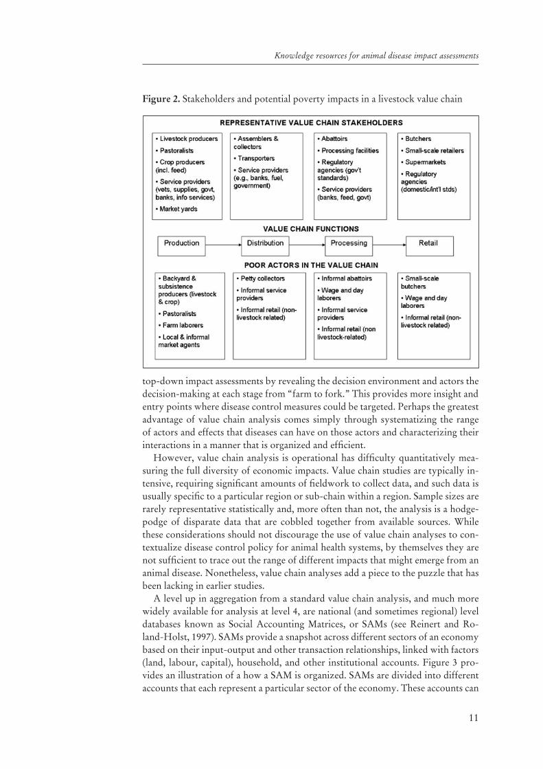
or more sophisticated techniques. For level 4, Rich and Perry (2010) and Rushton et al. (2009) point to value chain methodologies as useful for highlighting disease impacts across different sectors and pinpointing potential hotspots for disease risk. Figure 2 provides a schematic view of a representative value chain, including the stakeholders that could be affected by an animal disease outbreak. As such, value

approaches fail to capture. Moreover, value chain analysis goes beyond mapping interactions and stakeholders from production to consumption to assessing the in-stitutional contexts governing the organization of the chain. In particular, an im-portant component of value chain analysis addresses relationships within the chain

and incentives for disease control. Such a framework thus moves beyond the typical

11

Knowledge resources for animal disease impact assessments

top-down impact assessments by revealing the decision environment and actors the decision-making at each stage from “farm to fork.” This provides more insight and entry points where disease control measures could be targeted. Perhaps the greatest advantage of value chain analysis comes simply through systematizing the range of actors and effects that diseases can have on those actors and characterizing their

-suring the full diversity of economic impacts. Value chain studies are typically in-

rarely representative statistically and, more often than not, the analysis is a hodge-podge of disparate data that are cobbled together from available sources. While these considerations should not discourage the use of value chain analyses to con-textualize disease control policy for animal health systems, by themselves they are

animal disease. Nonetheless, value chain analyses add a piece to the puzzle that has been lacking in earlier studies.

A level up in aggregation from a standard value chain analysis, and much more widely available for analysis at level 4, are national (and sometimes regional) level databases known as Social Accounting Matrices, or SAMs (see Reinert and Ro-land-Holst, 1997). SAMs provide a snapshot across different sectors of an economy based on their input-output and other transaction relationships, linked with factors (land, labour, capital), household, and other institutional accounts. Figure 3 pro-vides an illustration of a how a SAM is organized. SAMs are divided into different accounts that each represent a particular sector of the economy. These accounts can

Figure 2. Stakeholders and potential poverty impacts in a livestock value chain

12

An assessment of the socio-economic impacts of global rinderpest eradicationFi

gure

3. S

truc

ture

of a

soc

ial a

ccou

ntin

g m

atri

x

1. A

ctiv

itie

s2.

Com

mod

itie

s3.

Fac

tors

4. P

riva

te

Hou

seho

lds

5. E

nter

pris

es6.

Rec

urre

nt

Sta

te7.

Inv

estm

ent

S

avin

gs8.

Res

t of

W

orld

9. T

otal

1. A

ctiv

itie

sM

arke

ted

Pro

duct

ion

Tot

al S

ales

2. C

omm

odit

ies

Inte

rmed

iate

C

onsu

mpt

ion

Pri

vate

C

onsu

mpt

ion

Stat

e C

onsu

mpt

ion

Inve

stm

ent

Exp

orts

Tot

al C

omm

odit

y D

eman

d

3. F

acto

rsV

alue

Add

edV

alue

Add

ed

4. P

riva

te

H

ouse

hold

sW

ages

, Sal

arie

s an

d O

ther

D

istr

ibut

ed

Soci

al

Secu

rity

Soci

al S

ecur

ity

and

Oth

er

Cur

rent

Tra

nsfe

rs

to H

ouse

hold

s

Net

For

eign

T

rans

fers

to

Hou

seho

lds

Pri

vate

H

ouse

hold

In

com

e

5. E

nter

pris

esN

et F

orei

gn

Tra

nsfe

rs to

E

nter

pris

es

Ent

erpr

ise

Inco

me

6. R

ecur

rent

S

tate

Indi

rect

Tax

esC

onsu

mpt

ion

Tax

es p

lus

Impo

rt T

arif

fs

Fac

tor

Tax

esIn

com

e T

axes

Ent

erpr

ise

Inco

me

Tax

esN

et F

orei

gn

Tra

nsfe

rs to

Stat

e

Stat

e R

even

ue

7. I

nves

tmen

S

avin

gsH

ouse

hold

Sa

ving

sR

etai

ned

Ear

ning

s &

E

nter

pris

e Sa

ving

s

Stat

e Sa

ving

sN

et C

apit

al

(=F

orei

gnSa

ving

s)

Tot

al S

avin

gs

8. R

est

of

Wor

ldIm

port

sIm

port

s

9. T

otal

Tot

al P

aym

ents

Tot

al

Com

mod

ity

Supp

ly

Tot

al F

acto

r P

aym

ents

Allo

cati

on o

f P

riva

te

Hou

seho

ld

Inco

me

Tot

al

Ent

erpr

ise

Exp

endi

ture

Allo

cati

on o

f St

ate

Rev

enue

Tot

al

Inve

stm

ent

Tot

al F

orei

gn

Exc

hang

e

Sour

ce: R

eine

rt a

nd R

olan

d-H

olst

(199

7).

13

Knowledge resources for animal disease impact assessments

be relatively aggregate (e.g., agriculture) or can disaggregate different sub-sectors (e.g., maize production, beef production, etc.). A SAM is principally an account-ing framework that traces income and expenditure between all these entities, e.g. revenues earned by a sector by the sales of goods and services it provides, and the expenditures made in producing that good or service. By construction, the principle of double-entry bookkeeping makes each agent’s total receipts (rows) equal to ex-penditures (columns).

-ties, commodities, factors, institutions, capital, and rest-of-the-world. Activities ac-counts are the productive sectors of the economy that sells goods (commodities) to the domestic market and export internationally, while buying raw materials and factors to produce such goods. Commodities represent domestic product markets,

-holds. A key distinction between activities and commodities is that activities are the actions that produce commodities, which are then sold to consumers. Factor markets include labour and capital markets that earn income from wages and rent, and pay salaries to households. Household accounts can be disaggregated by region and/or income level, thus providing insights on the links between the broader econ-omy and households. Institutions include households and government. Households receive income from factor accounts, and pay taxes and for commodities purchased in the economy. Households may also pay/receive transfers to other households or the government. Government is a separate institution, receiving income from taxes and tariffs, and paying out subsidies (on activities) and provides transfers. The capital account represents savings and investment in the economy, with investment

government. Finally, the rest of the world (ROW) account denotes international transactions in the terms of exports and imports of goods, services, and remittances.

As will be illustrated in more detail in the next section, a useful aspect of SAMs is their ability to be operationalized in a variety of applications. At their most basic level, SAMs can be used to construct a matrix of multipliers that highlight the de-

-ming from government spending, investment, or exports. These multipliers can provide insights on which sectors respond more towards investment than others. As noted earlier, Roeder and Rich (2009) found that the livestock sectors of East Africa had relatively high activity multipliers (between 3-5, meaning that a US$1 in-

to other sectors, suggesting that government spending in the sector (as in the case of

settings, Garner and Lack (1995), Ekboir (1999), and Mahul and Durand (2000) utilized SAMs in their analyses to measure the impacts of different interventions at a more macro level. SAMs can further be used as a database for more sophisticated computable general equilibrium (CGE) analyses that look more dynamically at the adjustment effects that could come from the shock of an animal disease (see Perry et al., 2003 and Diao, 2010 for examples).

By themselves, SAMs do not capture dynamics or price changes associated with

14

An assessment of the socio-economic impacts of global rinderpest eradication

assumed to be static (Reinert and Roland-Holst, 1997). However, dynamic adjust-ments will be a critical part of any analysis. These can be addressed in a SAM (see Miller and Blair, 1985 and the discussion in the next section), though not with the same level of sophistication as in other models. Partial equilibrium approaches (i.e., modelling supply and demand relationships at a sector level) allow the user to trace out the price and welfare impacts resulting from animal disease shocks (see Rich et al., 2005), with methods established to compute dynamic welfare measures of producer and consumer surplus in a multimarket setting (see Bullock et al., 1996 or Just et al., 2004) and to examine impacts on different household groups (Minot and Goletti, 1998). Rich and Winter-Nelson (2007) utilized such a dynamic partial equi-librium approach in the analysis of FMD. Such techniques, however, are relatively

and production effects associated with disease, while livelihood impacts are crudely modelled by income quartiles, for instance.

At a more macro-level than the SAM is a computable generally equilibrium -

havioral equations that capture the actions of agents within the economy (Sadoulet and de Janvry, 1995). Unlike SAMs, price effects are modeled, as are various types of sector and macroeconomic effects, including impacts on exchanges rates, gov-

applications (see Rich, Winter-Nelson and Miller, 2005 for a review). While CGE

details depending on the level of disaggregation within the SAM. In addition, liveli-hood impacts from a CGE analysis are restricted to the household accounts pro-vided in a given SAM as well.

Value chain approaches are useful in revealing behavioural changes that could arise from animal disease control or eradication that might have local or global spillovers, while CGE analyses can point to global impacts that highlight impacts of trade bans and other inter-regional phenomena. A combination of “level 4” methods probably comes

non-market methods and organizational behavioral models to assess the costs of spillovers associated with rinderpest.

Ultimately, the analysis of any animal disease phenomenon will include tradeoffs between economic sophistication, institutional detail, and data availability. A par-ticular need is to marry micro- and sector-level impacts with their broader effects on up and downstream markets within the value chain and with respect to other related and (seemingly) unrelated markets, and their resultant livelihood impacts. In the next section, we present a combination of sector-level, SAM, and CGE analyses to ex-post assessment of rinderpest control, providing details on the methodology and their application to the control and eradication of rinderpest in two case stud-ies, Chad and India.

15

ex-post

The thrust for our method is to conduct a broader ex-post of an animal health intervention at various levels of analysis. Our starting point is Golan et al. (2001) who adapted a SAM for the United States to examine the mac-roeconomic impacts of investments in food safety. In their analysis, the micro-level

of the economy were incorporated in a SAM multiplier analysis to gauge the to-

without rinderpest control programmes against the additional cost of rinderpest control campaigns. We further extend the analysis of Golan et al. (2001) by looking

exist in the absence of rinderpest control campaigns and comparing those impacts with the actual growth that occurred in the economy at large. This necessitates the

rinderpest eradication.In line with the levels of analysis provided in the previous section, the methodol-

ogy that we utilize adopts a sequential strategy in which the level of aggregation of

step based on outputs from the subsequent one. In particular, we do the following:First, define a counterfactual scenario in terms of the biological impacts of rin-derpest (with and without eradication campaigns) and their cost implications;Calculate and compare sector-level benefits in the livestock sector with and without rinderpest control, based on available price and production data, and simulation analysis of cattle production trends, thus trying to tease out an approximation of behavioral impacts resulting from rinderpest control (levels -3);Compute the additional costs associated with rinderpest control campaign, based on available data, comparing these costs to benefits and calculating a sector-level benefit-cost ratio;Compute multipliers from available SAMs to examine the growth linkages from rinderpest control, including a decomposition of multipliers to highlight paths of influence from economic shocks and their livelihood effects; and apply these to the sector-level BCR (level 4);Project long-run dynamic impacts from rinderpest control based on a CGE analysis, using the SAM in question and calibrated based on growth patterns and the counterfactual scenario (levels 4 and 6).

As an example of applying this methodology, we consider the case of rinderpest

16

An assessment of the socio-economic impacts of global rinderpest eradication

Chad

A major epidemic in 1913-1914 killed nearly 70 percent of cattle stocks, or about 1 million cattle. Rinderpest control did not begin in Chad until 1933 with the estab-lishment of vaccine centers in the country, and vaccination provided progressively improved control during the 1950s. However, as noted by Oussiguere (2010), bet-ter control through vaccination also coincided with lessened vigilance against the disease, leading to a rise in outbreaks in the late 1950s.

Internationally coordinated control efforts in Chad commenced with JP15 that began in September 1962. Between 1962 and 1970, outbreaks of rinderpest steadily

percent of cattle vaccinated in 1962, and fell erratically from 1963-1970 (Table 2). Vaccination coverage post-JP15 ranged between 29 percent and 44 percent during 1971 to 1977, then ceased during 1978-1982. A major outbreak in 1983, linked to movement of infected cattle, reportedly killed up to 337 500 head of cattle, after which vaccination coverage increased markedly in 1983 and 1984, before falling to a range of 43 percent to 54 percent between 1985 and 1988 (Oussiguere, 2010). The PARC programme, starting in Chad in 1989, ramped up vaccination coverage to over 76 percent by 1992, which was gradually reduced during the remainder of the decade as sero-surveillance programmes were established to verify the absence of infection.

For Chad, our counterfactual scenario assumes that in the absence of rinderpest control campaigns, the disease is primarily controlled via movement controls and targeted interventions upon the discovery of disease. This counterfactual largely characterizes control efforts pre-JP15 during the 1950s. Thus, this implies that the added costs from rinderpest campaigns can be assumed to be those spent by donors and national governments alike, over and beyond other ancillary disease control programmes.

-ing major outputs from the livestock sector: live animals, meat, and milk. These necessitate time-series data on production and prices, some of which is available on data sources in public domain such as FAOSTAT. To facilitate the comparison

Table 2. Rinderpest outbreaks during JP15 in Chad, 1963-1970

(%)

1963 33 980 716 22 83

1964 9 1,892 1,802 200 69

1965 7 658 257 37 40

1966 46 2,152 756 16 79

1967 39 967 660 17 41

1968 25 446 267 11 34

1969 26 927 516 20 32

1970 19 408 228 12 29

Average 26 1,054 650 42

Source: Oussiguere (2010)

17

A new methodological framework for the ex-post assessment of rinderpest eradication

of actual events with rinderpest control with the counterfactual scenario, in which rinderpest control campaigns were assumed not to have occurred, we utilize the DynMod simulation software (Lesnoff et al., 2007; 2008). DynMod projects the dynamic population behavior of cattle herds based on assumptions and observed data on herd demographics, offtake rates, death rates, and reproduction rates. Based on parameter assumptions provided in Lesnoff et al. (2008) and observations with FAOSTAT data on periods of production shocks (e.g., from droughts), we cali-brate DynMod to roughly reproduce the baseline production data reported from FAOSTAT. The counterfactual is constructed by adding the additional mortality engendered by rinderpest as observed from data pre-JP15, which provides an alter-native production projection. In the absence of information on price elasticities and because the magnitude of production differences are generally small, we assume that prices in both the “with” and “without” scenarios are the same.

We also considered the impact of morbidity as well in our calculations. From our data, we have information on both affected and dead animals, which allows us to construct a net morbidity percentage of surviving, affected animals. This percentage is used to adjust the volume of milk available from sick animals, as animals affected by rinderpest will have lower milk yields than healthy ones. We assumed that milk

is relatively small, but important in contexts where milk production is important (e.g., India).

Table 2 and Table 3 illustrate the computation of mortality rates attributed to the “without” case in Chad. Between 1963-1970, an average of 42 cattle were reported

number of outbreaks before JP15 (1958-1961) gives us an approximate number of animals that died because of rinderpest. Extrapolating population numbers back to

Table 3. Rinderpest outbreaks pre-JP15 in Chad, 1958-1961

1958 351 14,677 3,955,432 0.37 %

1959 367 15,346 4,012,786 0.38 %

1960 235 9,826 4,070,971 0.24 %

1961 324 13,548 4,130,000 0.33 %

Average 13,349 0.33 %

Additional outbreaks relative to 1963-1970 average

294 12,699 0.32%

Additional outbreaks relative to highest mor-tality rate during 1963-1970

0.08%

Additional outbreaks relative to lowest mor-tality rate during 1963-1970

1.54%

Source: Oussiguere (2010). * Populations for 1958-1960 extrapolated from 1.45% growth rate observed in the 1960s.

18

An assessment of the socio-economic impacts of global rinderpest eradication

the late 1950s using 1960s population growth trends provides us with total animal stocks that are used in Table 3 to calculate mortality rates associated with rinder-pest. This additional mortality is added to standard mortality rates in DynMod to provide an alternative population projection in the absence of rinderpest control. As a means of conducting some sensitivity analysis, we also calculated representa-tive “high” and “low” additional mortality in which the highest number of deaths per outbreak during 1963-1970 (200) and lowest number of deaths per outbreak (11) were used instead of the average and then applied to the 1950s data. This gives us a high additional mortality rate due to rinderpest of 1.54 percent and a low ad-ditional mortality rate of 0.08 percent. Additional sensitivity analysis whereby the mortality rate was incrementally increased by 0.05 was also conducted to determine the break-even BCR.

One of the challenges in calibrating the production data is accounting for various exogenous shocks to cattle populations, particularly those attributable to droughts. In Chad, major production shocks occurred in 1969, 1973-1974, and 1984 (Figure 4). The latter shock included a combination of drought with a major rinderpest outbreak that Oussiguere (2010) reported killing 337 500 cattle. To account for these shocks, we adjusted the standard mortality rates in DynMod to roughly approximate the observed trend. In a normal year, we assume that 11.2 percent of female calves (less than 1 year old) and 10.2 percent male calves die in a given year, while older animals die at a 5.8 percent rate for females and 5.2 percent for males. In 1969, we assumed that mortality rates increased by 50 percent. In 1973, mortality rates for males and females were assumed to be 35 percent for young stock and 15 percent for older stock; these were doubled in the major drought year of 1974. In 1984, we decomposed mortality (assumed at the same rates as 1974) into a drought shock and a rinderpest shock. The rinderpest shock accounted for about 35 percent of deaths in 1984. We assume that in the counterfactual case, these additional rinderpest deaths would not occur, as without control campaigns, there

Figure 4. Cattle population trends in Chad, 1963-2007

Source: FAOSTAT

19

would be low-level endemicity of disease that could preclude larger pandemics.Figure 5 illustrates the projected population trends with and without rinderpest

control as computed from DynMod, comparing the average, high, and low coun-terfactual cases. Interestingly, populations in the counterfactual are actually higher post-1984 for several years, though populations under the control case eventually

-trol would be lower in such years, highlighting the need for a much longer time

-pest mortality” case is particularly noteworthy in that cattle populations remain at depressed levels (2007 populations are slightly less than those in the early 1960s), whereas under “low rinderpest mortality,” populations are higher than under rin-derpest eradication.

Based on these projections, conversion rates for meat and milk, and offtake rates for domestic and export sales, we next compute values for the production of ani-mal, meat, and milk. Price data is not available for Chad, so we proxy price data

for 1991-2007. Data on cattle prices from 1968-1988 comes from the dataset used in Fafchamps and Gavian (1995), with conversion rates to meat and milk from live animal prices based on the methodology used in FAOSTAT. For 1963-1967, prices

World Bank’s World Development Indicators.The costs of rinderpest control in Chad were primarily extracted from the data

reported in Lepissier (1971) and Oussiguere (2010). Oussiguere (2010) cites the number of vaccinations administered during JP15 and post-JP15 until 1988, but

Figure 5. Chad: baseline case.

A new methodological framework for the ex-post assessment of rinderpest eradication

20

An assessment of the socio-economic impacts of global rinderpest eradication

does not give a cost estimate. Lepissier (1971) estimates that the unit costs of vac-cine administration in Chad based on aggregate JP15 expenditures were 59.8 CFA, of which 30.1 CFA are attributed to international donor funds and 28.9 CFA are

constant real 2 000 CFA) to the number of vaccinations applied based on Ous-siguere (2010). Between 1971-1988, we assume that the real unit cost of vaccination is the national cost component provided in Lepissier (1971) of 28.9 CFA. For the costs of the PARC and PACE programmes, Oussiguere (2010) reports aggregate costs associated with both programmes. As an approximation, we assumed that these funds were divided evenly in each year of the respective programme. All costs

by the World Bank.

were available, looking at three scenarios (baseline, high mortality, and low mortality), with assumptions on additional mortality due to rinderpest found in

1994 were negative based on our assumption that rinderpest pandemics would be lessened in the presence of constant endemicity, thus providing a very conservative estimate of the impacts of rinderpest control.

above the BCRs of 1.06-3.84 reported in Tambi et al. (1999) that evaluated the -

sensitive to the choice of scenario considered and in particular the mortality rate.

-riod. This is due entirely to the marked variation in population levels, which under higher levels of rinderpest mortality are much lower than under eradication (see

cost ratio is actually negative by virtue of impact of the 1983-84 drought. In the low rinderpest mortality case, mortality during the drought is lower than eradica-tion, and population growth rates under eradication and this scenario are nearly the same. This implies that populations post-drought in the low mortality scenario are actually higher. However, if we look at BCRs pre-drought (1963-1983) in this low

-derstand the differential impacts of mortality stemming for drought and rinderpest both.

In Figure 7, we conducted a sensitivity analysis to map the relationship between -

sis, we also considered the sensitivity of the BCR to the percentage of deaths associ-ated with rinderpest during the 1984 drought. In the baseline, as mentioned above, we assumed that 35 percent of deaths were due to rinderpest in the 1984 drought. In the sensitivity analysis, we consider the impacts on the BCR if that percentage

21

Table 4. (billion CFA, 2000 prices)

Costs

1963 0.072 0.35 0.018 1.149

1964 0.601 2.89 0.150 0.953

1965 0.712 3.39 0.178 0.566

1966 0.865 4.10 0.217 1.132

1967 0.826 3.88 0.207 0.587

1968 0.831 3.87 0.209 0.500

1969 0.923 4.23 0.233 0.451

1970 2.431 11.27 0.612 0.416

1971 2.025 9.29 0.511 0.312

1972 3.326 15.23 0.840 0.258

1973 0.267 -1.91 0.721 0.286

1974 1.414 2.59 1.173 0.160

1975 8.147 31.29 3.314 0.205

1976 9.717 37.72 3.811 0.231

1977 7.779 30.52 2.919 0.170

1978 6.140 24.23 2.222 0.000

1979 8.536 33.57 3.106 0.000

1980 7.686 30.27 2.737 0.000

1981 14.753 57.93 5.312 0.000

1982 15.008 58.94 5.316 0.000

1983 3.384 13.31 1.051 0.884

1984 -41.624 -54.20 -38.862 0.350

1985 -0.264 17.17 -4.184 0.241

1986 -7.304 59.13 -22.146 0.246

1987 -0.516 28.83 -7.231 0.323

1988 -1.068 33.01 -8.883 0.305

1989 -2.670 57.64 -16.489 0.324

1990 -1.223 51.33 -13.389 0.297

1991 -0.747 56.91 -14.185 0.287

1992 0.746 48.43 -10.546 0.326

1993 1.216 48.71 -10.115 0.320

1994 0.335 100.56 -23.316 0.793

1995 1.781 74.13 -15.526 0.721

1996 2.326 56.93 -10.905 0.640

1997 2.949 66.24 -12.446 0.630

1998 3.346 61.53 -10.933 0.589

1999 4.283 68.81 -11.676 1.425

2000 4.943 74.07 -12.241 0.750

2001 5.178 71.90 -11.507 0.657

2002 5.757 72.77 -11.136 0.647

NPV@5% 32.46 380.89 -47.06 8.08

BCR 4.02 47.15 -5.83

A new methodological framework for the ex-post assessment of rinderpest eradication

22

An assessment of the socio-economic impacts of global rinderpest eradication

-tions on the additional mortality associated with rinderpest as well as the drought impact, suggesting the need for careful research on these mortality-related effects.

The next step in the analysis is to examine the economywide impacts of rin-derpest control. This necessitates analysis with a social accounting matrix that was developed for Chad (Garber, 2009). The structure of accounts in the Chad SAM is given in Table 5. We start by conducting a standard multiplier analysis by generat-ing a multiplier matrix and then applying this to a hypothetical vector of exogenous shocks based on our “with” and “without” scenarios. It is instructive to review how this is accomplished in a SAM. Let A be an n X nof productive, endogenous sectors in the SAM, where the entry aij is the amount of sector i used in the production of sector j’s output, Xij (Sadoulet and de Janvry, 1995). Let X be an n X 1 vector of outputs of endogenous sectors, and let F be an n X 1of outputs from government accounts, capital accounts, and rest-of-the-world ac-counts. Then, in matrix form, the relationships in our SAM can be written as:

the following equation, with the inverse of the expression (I-A) is what is known as the multiplier matrix:

The multiplier matrix, as noted earlier, tells us how much output is generated

Figure 6. Comparison of cattle population projections with and without rinder-pest control under different scenarios, 1963-2

Source: Model simulations with DynMod

XFAX

XFAI 1)(

23

-gendered by this:

XFAI 1)( (3)

Table 6 and Table 7 provide multipliers associated with a number of agricultural

are provided. We read the multipliers down each column as follows, taking the livestock activity column as an example. In this case, a one-unit increase in government spending on livestock production activities would lead to an increase in total productive output of 3.49 units, domestic supply of 3.73 units, factors of production of 2.48 units, and household income of 2.62 units (Table 6). Commodity multipliers for livestock are similar in magnitude, though domestic supply increases more (4.63) relative to a one-unit shock to livestock production (Table 7). Agricultural activity and commodity multipliers tend to be higher than industrial ones (with the exception of cotton milling), while household multipliers are much higher for injections into agriculture than industry, suggesting greater income generation potential from agriculture. Household multipliers for livestock

enterprises than other agriculture activities. These multipliers suggest that the net

with rinderpest control is much higher. As a very crude approximation, applying

Figure 7. -ferent mortality rates and percentage of rinderpest deaths associated with drought.

Source: Model simulations with DynMod. Note: the “BCR @” labels refer to the percentage of 1984 drought deaths associated with rinderpest. The baseline assumes 35 percent of deaths in 1984 were rinderpest-related, which is relaxed in the sensitivity analysis illustrated above.

A new methodological framework for the ex-post assessment of rinderpest eradication

24

An assessment of the socio-economic impacts of global rinderpest eradication

Table 5. Accounts in the Chad social accounting matrix (2000)

Aag Agriculture (activities)

Aagcot Cotton crops (activities)

Alive Livestock (activities)

Fisheries (activities)

Aman Manufacturing (activities)

Acot

Adev Oil development (activities)

Acon Construction (activities)

Ainf Informal manufacturing (activities)

Aserv Services (activities)

Agov Government (activities)

Cag Agriculture (commodities)

Cagcot Cotton crops (commodities)

Clive Livestock (commodities)

Fisheries (commodities)

Cman Manufacturing (commodities)

Ccot

Cdev Oil development (commodities)

Ccon Construction (commodities)

Cinf Informal manufacturing (commodities)

Cserv Services (commodities)

Cgov Government (commodities)

Fland Land (factor accounts)

Fcapf Capital, formal sector (factor accounts)

Fcapl Capital, informal sector (factor accounts)

Flabp Labour, privileged sector (factor accounts)

Flabn Labour, non-privileged sector (factor accounts)

Hrurag Rural agricultural households (households)

Hrurpub Rural public sector (households)

Hurbinf Urban informal sector (households)

Hurbcr Urban capitalist-rentier (households)

Hurbpub Urban public sector (households)

Hurbw Urban wage workers (households)

Hent Enterprises (households) Source: Garber (2009)

the commodity multiplier of 4.63 to the BCR at a sector-level gives an aggregate BCR of well over 18.

Multipliers can be further decomposed to determine the paths of transmission of economy activity to assess who gains (and how) from the added-value generated in the economy. Following techniques developed in Defourny and Thorbecke (1984) and applied by Roland-Holst and Otte (2007) in the context of livestock and livelihood

25

Tab

le 6

. Act

ivit

y m

ulti

plie

rs fo

r C

had

Agr

icul

ture

1.60

0.59

0.53

0.55

0.39

0.49

0.27

0.32

0.38

0.38

0.35

Cot

ton

0.00

1.00

0.00

0.00

0.00

0.71

0.00

0.00

0.00

0.00

0.00

Liv

esto

ck0.

250.

251.

220.

230.

630.

210.

170.

190.

220.

180.

19

Fis

heri

es0.

060.

060.

061.

100.

040.

050.

070.

200.

060.

050.

05

Man

ufac

turi

ng0.

350.

350.

330.

351.

370.

300.

310.

350.

370.

310.

33

Cot

ton

mill

ing

0.00

0.00

0.00

0.00

0.00

1.00

0.00

0.00

0.00

0.00

0.00

Oil

deve

lopm

ent

0.00

0.00

0.00

0.00

0.00

0.00

1.00

0.00

0.00

0.00

0.00

Con

stru

ctio

n0.

010.

010.

010.

010.

010.

010.

231.

020.

010.

010.

02

Info

rmal

act

ivit

ies

0.31

0.31

0.30

0.31

0.20

0.26

0.14

0.18

1.32

0.19

0.20

Serv

ices

0.99

0.99

1.03

0.99

0.91

1.04

1.16

1.01

0.93

2.05

0.98

Gov

ernm

ent

0.01

0.01

0.01

0.01

0.01

0.01

0.00

0.01

0.01

0.01

1.01

TO

TA

L A

CT

IVIT

Y3.

583.

573.

493.

553.

574.

093.

353.

283.

293.

183.

13

Agr

icul

ture

0.80

0.79

0.71

0.74

0.52

0.66

0.36

0.43

0.51

0.51

0.46

Cot

ton

0.00

0.00

0.00

0.00

0.00

0.72

0.00

0.00

0.00

0.00

0.00

Liv

esto

ck0.

270.

270.

230.

240.

680.

230.

180.

210.

230.

190.

21

Fis

heri

es0.

080.

080.

080.

130.

060.

070.

090.

270.

070.

060.

06

Man

ufac

turi

ng1.

041.

041.

001.

051.

100.

910.

931.

051.

120.

940.

99

Cot

ton

mill

ing

0.00

0.00

0.00

0.00

0.00

0.00

0.00

0.00

0.00

0.00

0.00

Oil

deve

lopm

ent

0.00

0.00

0.00

0.00

0.00

0.00

0.00

0.00

0.00

0.00

0.00

Con

stru

ctio

n0.

010.

010.

010.

010.

010.

010.

230.

020.

010.

010.

02

Info

rmal

act

ivit

ies

0.32

0.32

0.30

0.32

0.20

0.26

0.14

0.18

0.33

0.20

0.21

Serv

ices

1.32

1.32

1.37

1.31

1.22

1.39

1.55

1.34

1.23

1.40

1.31

Gov

ernm

ent

0.01

0.01

0.01

0.01

0.01

0.01

0.00

0.01

0.01

0.01

0.01

TO

TA

L C

OM

MO

DIT

Y3.

853.

843.

733.

823.

794.

273.

493.

503.

513.

313.

26

cont

.

A new methodological framework for the ex-post assessment of rinderpest eradication

26

An assessment of the socio-economic impacts of global rinderpest eradication

Lan

d0.

240.

240.

400.

220.

220.

190.

080.

100.

100.

090.

09

Cap

ital

, for

mal

se

ctor

0.10

0.10

0.10

0.10

0.17

0.20

0.21

0.19

0.09

0.16

0.29

Cap

ital

, inf

orm

al

sect

or0.

380.

380.

390.

380.

380.

390.

410.

410.

570.

680.

36

Lab

or, p

rivi

lege

d se

ctor

0.05

0.05

0.06

0.05

0.08

0.08

0.09

0.13

0.05

0.10

0.30

Lab

or, n

on-p

rvi-

lege

d se

ctor

1.70

1.71

1.54

1.75

0.99

1.38

0.66

0.83

1.08

0.89

0.83

TO

TA

L F

AC

TO

R2.

462.

482.

482.

501.

842.

231.

451.

661.

901.

931.

87

Rur

al a

gric

ultu

ral

1.11

1.12

1.10

1.13

0.71

0.91

0.47

0.58

0.73

0.64

0.57

Rur

al p

ublic

sec

tor

0.17

0.17

0.18

0.17

0.12

0.15

0.08

0.11

0.11

0.10

0.16

Urb

an in

form

al

sect

or0.

280.

290.

260.

290.

180.

240.

130.

160.

210.

190.

15

Urb

an c

apit

alis

t-re

ntie

r0.

180.

180.

170.

190.

110.

150.

080.

100.

130.

120.

10

Urb

an p

ublic

sec

-to

r0.

280.

290.

260.

290.

190.

250.

140.

180.

190.

180.

26

Urb

an w

age

wor

k-er

s0.

150.

150.

140.

150.

100.

130.

080.

110.

100.

100.

16

Ent

erpr

ises

0.43

0.44

0.52

0.43

0.48

0.50

0.47

0.46

0.50

0.62

0.50

TO

TA

L H

OU

SEH

OL

D2.

612.

622.

622.

641.

902.

321.

461.

701.

971.

961.

90So

urce

: Com

pute

d fr

om 2

000

Cha

d SA

M o

f Gar

ber

(200

9)

Tab

le 6

. Con

t.d

27

Tab

le 7

. Com

mod

ity

mul

tipl

iers

for

Cha

d

Agr

icul

ture

1.24

0.58

0.51

0.48

0.20

0.48

0.26

0.31

0.37

0.29

0.34

Cot

ton

0.00

0.98

0.00

0.00

0.00

0.69

0.00

0.00

0.00

0.00

0.00

Liv

esto

ck0.

220.

241.

150.

200.

240.

210.

160.

190.

210.

140.

19

Fis

heri

es0.

050.

060.

060.

850.

020.

050.

070.

200.

050.

030.

05

Man

ufac

turi

ng0.

310.

340.

320.

320.

510.

300.

300.

340.

360.

230.

32

Cot

ton

mill

ing

0.00

0.00

0.00

0.00

0.00

0.98

0.00

0.00

0.00

0.00

0.00

Oil

deve

lopm

ent

0.00

0.00

0.00

0.00

0.00

0.00

0.98

0.00

0.00

0.00

0.00

Con

stru

ctio

n0.

010.

010.

010.

010.

010.

010.

220.

990.

010.

010.

02

Info

rmal

act

ivit

ies

0.26

0.30

0.28

0.27

0.10

0.25

0.14

0.17

1.29

0.14

0.20

Serv

ices

1.04

0.97

1.03

1.09

0.66

1.02

1.14

0.98

0.91

1.54

0.96

Gov

ernm

ent

0.01

0.01

0.01

0.01

0.00

0.01

0.00

0.01

0.01

0.00

0.98

TO

TA

L A

CT

IVIT

Y3.

133.

493.

373.

231.

744.

003.

283.

203.

212.

393.

06

Agr

icul

ture

1.67

0.77

0.68

0.65

0.26

0.65

0.35

0.42

0.50

0.38

0.45

Cot

ton

0.00

1.00

0.00

0.00

0.00

0.71

0.00

0.00

0.00

0.00

0.00

Liv

esto

ck0.

230.

261.

220.

210.

260.

220.

170.

200.

230.

140.

20

Fis

heri

es0.

070.

080.

081.

110.

030.

070.

090.

260.

070.

050.

06

Man

ufac

turi

ng0.

921.

020.

970.

961.

530.

890.

911.

021.

090.

700.

96

Cot

ton

mill

ing

0.00

0.00

0.00

0.00

0.00

1.00

0.00

0.00

0.00

0.00

0.00

Oil

deve

lopm

ent

0.00

0.00

0.00

0.00

0.00

0.00

1.00

0.00

0.00

0.00

0.00

Con

stru

ctio

n0.

010.

010.

010.

010.

010.

010.

231.

020.

010.

010.

02

Info

rmal

act

ivit

ies

0.26

0.31

0.29

0.28

0.10

0.26

0.14

0.18

1.32

0.15

0.20

Serv

ices

1.38

1.29

1.37

1.45

0.88

1.36

1.51

1.31

1.21

2.05

1.28

Gov

ernm

ent

0.01

0.01

0.01

0.01

0.00

0.01

0.00

0.01

0.01

0.00

1.01

TO

TA

L C

OM

MO

DIT

Y4.

554.

754.

634.

673.

075.

174.

414.

424.

433.

494.

19

cont

.

A new methodological framework for the ex-post assessment of rinderpest eradication

28

An assessment of the socio-economic impacts of global rinderpest eradication

Lan

d0.

190.

230.

380.

180.

090.

180.

080.

100.

100.

070.

09

Cap

ital

, for

mal

sec

tor

0.10

0.09

0.10

0.10

0.09

0.20

0.21

0.19

0.09

0.12

0.28

Cap

ital

, inf

orm

al

sect

or0.

380.

370.

390.

400.

240.

380.

400.

400.

560.

510.

35

Lab

or, p

rivi

lege

d

sect

or0.

050.

050.

050.

060.

040.

080.

090.

130.

050.

070.

30

Lab

or, n

on-p

rivi

lege

d se

ctor

1.39

1.67

1.47

1.48

0.49

1.35

0.65

0.81

1.06

0.67

0.81

TO

TA

L F

AC

TO

R2.

122.

422.

392.

220.

952.

181.

421.

621.

861.

451.

83

Rur

al a

gric

ultu

ral

0.92

1.09

1.06

0.96

0.35

0.89

0.46

0.56

0.72

0.48

0.56

Rur

al p

ublic

sec

tor

0.14

0.17

0.17

0.15

0.06

0.14

0.08

0.11

0.10

0.08

0.15

Urb

an in

form

al s

ecto

r0.

240.

280.

250.

250.

090.

230.

130.

150.

200.

140.

15

Urb

an c

apit

alis

t-re

ntie

r0.

150.

180.

160.

160.

060.

150.

080.

100.

130.

090.

10

Urb

an p

ublic

sec

tor

0.24

0.28

0.25

0.25

0.09

0.24

0.14

0.18

0.18

0.14

0.25

Urb

an w

age

wor

kers

0.12

0.14

0.13

0.13

0.05

0.13

0.08

0.10

0.10

0.08

0.16

Ent

erpr

ises

0.42

0.43

0.50

0.43

0.27

0.48

0.46

0.45

0.49

0.47

0.49

TO

TA

L H

OU

SEH

OL

D2.

232.

562.

522.

340.

972.

271.

431.

661.

921.

471.

85 S

ourc

e: C

ompu

ted

from

200

0 C

had

SAM

of G

arbe

r (2

009)

Tab

le 7

. con

t.d

29

found in the SAM (Table 8). The data indicates that, with the exception of rural public sector groups, shocks to livestock supply are modulated through manufacturing activities, suggesting more complex interactions within the value chain that one

We can further use our SAM using the methodology employed by Thorbecke

vectors were generated and multiplied by the multiplier matrix to examine the im-pacts of alternative structural adjustment policies in Indonesia. This type of analysis

a particular, discrete time period, though is less suitable for a longer-run analysis given issues concerning the stability of multiplier matrix and potential price adjust-

(Miller and Blair, 1985).2

the situation without rinderpest control. To simulate this for the year 2000, we as-

-pest control in 2000 were calculated at 4.94 billion CFA. We can think of this shock as a loss in private investment in the economy suffered by those in the livestock value chain. In the Chad SAM, we simulate this by reducing investment by rural agricultural households by 4.94 billion CFA (i.e., the intersection in the “Caphetot” account column and “Hrurag” account row). For costs associated with this policy, we assume that there is a reduction in government spending on the livestock sector (production activity) in the amount of the control programmes in that year (750 million CFA). However, as government spending is fungible, we assume that the 750 million CFA that is not spent on livestock is reallocated in proportion to the structure of government spending given in the Chad SAM.

Table 9 provides an estimate of the sector-by-sector changes in output associ-ated with the counterfactual scenario in 2000, the base year of the SAM. The results show lower levels of production and income associated with the absence of rinder-pest control. Rural incomes in 2000 are 2.6 percent lower relative to the baseline cost in which rinderpest control takes place, while other household groups have

on a production basis occur in the agricultural sector (-1.7 percent), manufacturing (-1 percent), and the informal sector (-1.5 percent), all of which suggest that rinder-pest control has strong poverty reduction impacts in these sectors where broader-based employment opportunities exist. Measuring GDP at factor cost reveals that in the absence of rinderpest control, GDP would be 1 percent lower compared to the case with rinderpest control.

2 Golan et al. (2001) adopt this approach in the context of HAACP control in which they use the SAM to simu-

the shocks conceived relative to their SAM accounts are small whereas adopting a similar approach using the

A new methodological framework for the ex-post assessment of rinderpest eradication

30

An assessment of the socio-economic impacts of global rinderpest eradicationT

able

8. P

ath

deco

mpo

siti

on fo

r ho

useh

old

grou

ps in

Cha

d

Hru

rag

Cliv

e0.

241

0.02

41.

959

0.04

719

.319

.3

Hru

rag

Cag

Aag

Cliv

e0.

009

2.31

60.

021

8.5

27.9

Hru

rag

Cm

anA

man

Cliv

e0.

025

2.46

70.

0625

.152

.9

Hru

rag

Cin

fA

inf

Cliv

e0.

001

2.29

90.

003

1.1

54

Hru

rag

Cag

Aag

Cm

anA

man

Cliv

e0.

002

2.87

50.

007

2.8

56.8

Hru

rag

Cag

Aag

Fla

ndH

rurp

ubC

live

0.00

12.

352

0.00

20.

657

.5

Hru

rag

Cag

Aag

Fla

bnH

rurp

ubC

live

0.00

32.

538

0.00

83.

260

.7

Hru

rag

Cin

fA

inf

Cm

anA

man

Cliv

e0.

005

2.87

10.

015

6.1

66.8

Hru

rag

Cin

fA

inf

Fla

bnH

rurp

ubC

live

0.00

12.

647

0.00

10.

667

.3

Hru

rag

Cse

rvA

serv

Cm

anA

man

Cliv

e0.

004

3.63

0.01

66.

673

.9

Hru

rpub

Cliv

e0.

405

0.19

51.

292

0.25

262

.262

.2

Hru

rpub

Hru

rag

Cliv

e0.

001

2.03

20.

001

0.3

62.5

Hru

rpub

Cag

Aag

Cliv

e0.

006

1.91

90.

011

2.7

65.2

Hru

rpub

Cm

anA

man

Cliv

e0.

025

1.69

0.04

210

.475

.6

Hru

rpub

Cin

fA

inf

Cliv

e0.

001

1.61

40.

002

0.4

76

Hru

rpub

Hru

rag

Cm

anA

man

Cliv

e0.

001

2.54

30.

001

0.4

76.3

Hru

rpub

Hur

bwC

man

Am

anC

live

0.00

11.

822

0.00

20.

576

.8

Hru

rpub

Cag

Aag

Cm

anA

man

Cliv

e0.

002

2.42

0.00

40.

977

.7

Hru

rpub

Cag

Aag

Fla

bnH

rura

gC

live

0.00

22.

538

0.00

40.

978

.7

Hru

rpub

Cin

fA

inf

Cm

anA

man

Cliv

e0.

005

2.07

20.

012.

581

.2

Hru

rpub

Cse

rvA

serv

Cm

anA

man

Cliv

e0.

004

2.70

10.

012

2.9

84.1

cont

.

31

Hur

binf

Hru

rag

Cliv

e0.

225

0.00

12.

109

0.00

20.

90.

9

Hur

binf

Cag

Aag

Cliv

e0.

005

1.96

90.

011

4.8

5.7

Hur

binf

Cm

anA

man

Cliv

e0.

053

1.76

0.09

341

.347

Hur

binf

Cin

fA

inf

Cliv

e0.

001

1.67

10.

002

1.1

48.1

Hur

binf

Hru

rag

Cm

anA

man

Cliv

e0.

001

2.61

50.

003

1.2

49.3

Hur

binf

Hur

bwC

man

Am

anC

live

0.00

21.

891

0.00

41.

650

.9

Hur

binf

Cag

Aag

Cm

anA

man

Cliv

e0.

001

2.46

20.

004

1.6

52.5

Hur

binf

Cag

Aag

Fla

bnH

rura

gC

live

0.00

12.

554

0.00

41.

654

.1

Hur

binf

Cag

Aag

Fla

bnH

rurp

ubC

live

0.00

22.

264

0.00

41.

956

Hur

binf

Cin

fA

inf

Cm

anA

man

Cliv

e0.

007

2.12

20.

014

6.3

62.3

Hur

binf

Cin

fA

inf

Fla

bnH

rura

gC

live

0.00

12.

650.

001

0.6

62.9

Hur

binf

Cin

fA

inf

Fla

bnH

rurp

ubC

live

0.00

12.

320.

002

0.7

63.6

Hur

binf

Cse

rvA

serv

Cm

anA

man

Cliv

e0.

002

2.78

0.00

72.

966

.5

Hur

bcr

Hru

rag

Cliv

e0.

225

0.00

12.

043

0.00

20.

90.

9

Hur

bcr

Cag

Aag

Cliv

e0.

002

1.94

90.

004

1.8

2.7

Hur

bcr

Cm

anA

man

Cliv

e0.

065

1.69

20.

1148

.851

.5

Hur

bcr

Cin

fA

inf

Cliv

e0.

002

1.60

70.

003

1.4

52.9

Hur

bcr

Hru

rag

Cm

anA

man

Cliv

e0.

001

2.54

30.

003

1.2

54.1

Hur

bcr

Hur

bwC

man

Am

anC

live

0.00

21.

822

0.00

41.

655

.6

Hur

bcr

Cag

Aag

Cm

anA

man

Cliv

e0.

001

2.44

40.

001

0.6

56.2

Hur

bcr

Cag

Aag

Fla

bnH

rura

gC

live

0.00

12.

548

0.00

10.

656

.8

Hur

bcr

Cag

Aag

Fla

bnH

rurp

ubC

live

0.00

12.

259

0.00

20.

757

.6

cont

.

Tab

le 8

. Con

t.d

A new methodological framework for the ex-post assessment of rinderpest eradication

32

An assessment of the socio-economic impacts of global rinderpest eradication

Hur

bcr

Cin

fA

inf

Cm

anA

man

Cliv

e0.

009

2.05

30.

018

865

.5

Hur

bcr

Cin

fA

inf

Fla

bnH

rura

gC

live

0.00

12.

642

0.00

20.

866

.4

Hur

bcr

Cin

fA

inf

Fla

bnH

rurp

ubC

live

0.00

12.

312

0.00

20.

967

.3

Hur

bcr

Cse

rvA

serv

Cm

anA

man

Cliv

e0.

003

2.70

50.

008

3.4

70.6

Hur

bwH

rura

gC

live

0.21

50.

001

2.11

10.

002

0.8

0.8

Hur

bwC

agA

agC

live

0.00

61.

997

0.01

25.

66.

4

Hur

bwC

man

Am

anC

live

0.04

61.

751

0.08

137

.544

Hur

bwC

inf

Ain

fC

live

0.00

11.

674

0.00

21.

145

Hur

bwH

rura

gC

man

Am

anC

live

0.00

12.

633

0.00

21

46.1

Hur

bwC

agA

agC

man

Am

anC

live

0.00

22.

511

0.00

41.

948

Hur

bwC

agA

agF

labn

Hru

rag

Cliv

e0.

002

2.63

40.

004

249

.9

Hur

bwC

agA

agF

labn

Hru

rpub

Cliv

e0.

002

2.33

40.

005

2.2

52.2

Hur

bwC

inf

Ain

fC

man

Am

anC

live

0.00

62.

142

0.01

36.

358

.5

Hur

bwC

inf

Ain

fF

labn

Hru

rpub

Cliv

e0.

001

2.39

70.

002

0.7

59.2

Hur

bwC

serv

Ase

rvC

man

Am

anC

live

0.00

32.

801

0.00

73.

462

.6

Hen

tC

serv

Ase

rvC

agA

agC

live

0.12

40.

001

3.14

90.

002

1.7

1.7

Hen

tC

serv

Ase

rvC

man

Am

anC

live

0.01

92.

634

0.05

141

.142

.8

Hen

tC

serv

Ase

rvF

capl

Hru

rag

Cliv

e0.

001

3.22

30.

002

1.6

44.4

Hen

tC

serv

Ase

rvF

labp

Hru

rpub

Cliv

e0.

002

2.38

90.

004

2.9

47.3

Hen

tC

serv

Ase

rvF

labn

Hru

rag

Cliv

e0.

001

3.60

90.

005

4.1

51.3

Hen

tC

serv

Ase

rvF

labn

Hru

rpub

Cliv

e0.

002

3.19

40.

006

4.6

55.9

Sour

ce:

Tab

le 8

. Con

t.d

33

Long Term Impacts of Livestock DiseaseBecause of the relatively long and varied history of rinderpest control around the

countries have differing levels of livestock dependence as a percent of economic

countries livestock can be a very important contributor to formal sector income (Figure 8).

To give general indications of long-term impact of Rinderpest eradication on lower income economies, we use two types of forecasting models, one for a single country and a global model. The individual country is again Chad, as it is thought to represent a relatively livestock dependent low-income economy with reliable data. For the global model, we aggregate the GTAP 7 database to detail 19 regions and 12 sectors.

In both cases, the counterfactual for a world without Rinderpest eradication is

relative vulnerability of lower income countries to recurrent incidence of such ani-mal diseases. Using an elasticity scenario, we assume that livestock productivity in the counterfactual declines 1 percent annually, and then examine changes in annual macroeconomic aggregates over a twenty-year period (2010-2030). Data constraints prevent of from doing historical counterfactuals, but the pattern of vulnerabilities is thought to be representative of today’s livelihood and livestock economy condi-tions.

Table 10 presents results for average annual changes in Chad’s real macroeco-nomic aggregates under two scenarios designed to be indicative of recurrent live-stock disease like Rinderpest:

1. Livestock sector productivity declines 1percent annually from 2010 to 2030.2. Because of endemic disease burdens (repeat the above two scenarios), we

assume Chadian livestock exports are reduced by 50 percent.These results show how important livestock production is across the Chad-

ian economy, but particularly for household livelihoods and purchasing power. If Livestock productivity sustained just 1 percent annual declines, as might result from the mortality and stunting associated with endemic Rinderpest, over two de-cades national income would be 15 percent lower, real consumption 17 percent lower, driving many vulnerable poor families over the threshold to destitution and malnutrition. If trade partners reacted to the disease emergence, as they often do, by restricting trade in livestock products, the adverse effects would be even more serious.

Real output results suggest the structural adjustments that would ensue from livestock sector linkages across the economy. For example, as a competitor for ag-

Manufacturing, with a large component of food processing, is particularly hard hit,

sector is hit by reduced aggregate growth. Analogous results would doubtless be obtained by assessments of other livestock dependent low-income countries, else-where in Africa and globally.

A new methodological framework for the ex-post assessment of rinderpest eradication

34

An assessment of the socio-economic impacts of global rinderpest eradication

Table 9. Simulated economywide impacts of rinderpest control in 2000, billion CFA (2000 prices)

Aag 0.00 -3.55 205.18 201.63 -1.73 %

Aagcot 0.00 0.00 27.04 27.04 0.00 %

Alive -0.75 -1.89 190.54 188.65 -0.99 %

0.00 -0.32 36.67 36.35 -0.88 %

Aman 0.00 -1.66 164.69 163.03 -1.01 %

Acot 0.00 0.00 38.21 38.21 0.00 %

Adev 0.00 0.00 18.19 18.19 0.00 %

Acon 0.00 -0.06 57.38 57.32 -0.10 %

Ainf 0.00 -1.71 117.28 115.58 -1.46 %

Aserv 0.00 -5.29 532.34 527.05 -0.99 %

Agov 0.00 0.59 191.07 191.66 0.31 %

Cag 0.00 -4.77 275.50 270.73 -1.73 %

Cagcot 0.00 0.00 27.69 27.69 0.00 %

Clive 0.00 -1.21 202.77 201.56 -0.60 %

0.00 -0.42 48.04 47.61 -0.88 %

Cman 0.00 -4.98 493.67 488.69 -1.01 %

Ccot 0.00 0.00 39.09 39.09 0.00 %

Cdev 0.00 0.00 18.62 18.62 0.00 %

Ccon 0.00 -0.06 58.76 58.70 -0.10 %

Cinf 0.00 -1.75 120.15 118.40 -1.46 %

Cserv 0.00 -7.04 708.52 701.49 -0.99 %

Cgov 0.64 0.61 195.48 196.08 0.31 %

Fland 0.00 -0.92 80.08 79.16 -1.14 %

Fcapf 0.00 -0.38 97.29 96.92 -0.39 %

Fcapl 0.00 -2.04 196.43 194.39 -1.04 %

Flabp 0.00 -0.12 79.96 79.83 -0.16 %

Flabn 0.00 -5.63 500.34 494.71 -1.12 %

Hrurag -4.88 -9.27 358.99 349.72 -2.58 %

Hrurpub 0.01 -0.55 70.57 70.02 -0.78 %

Hurbinf 0.00 -1.00 90.79 89.79 -1.11 %

Hurbcr 0.00 -0.64 58.27 57.63 -1.11 %

Hurbpub 0.02 -0.90 113.88 112.97 -0.79 %

Hurbw 0.01 -0.46 66.35 65.88 -0.70 %

Hent 0.01 -2.06 241.39 239.33 -0.85 %

Source: Simulations using the Chad SAM of Garber (2009)

Next we examine the same issue globally, using a GTAP-based dynamic CGE model to examine two counterfactual scenarios:

1. Livestock sector productivity declines 1 percent annually from 2010 to 2030, in low-income countries only.

35

Figure 8. National livestock dependence, West Africa

Table 10. Macroeconomic impacts of livestock sector scenarios for Chad (percentage change from Baseline values in 2030)

Real GDP -15% -14%

HH Income -15% -18%

Consumption -17% -19%

Exports -11% -9%

Imports -7% -9%

Real Output

Agriculture -6% -6%

Cotton crops 2% 3%

Livestock -27% -28%

Fisheries -6% -5%

Manufacturing -28% -24%

Cotton Fib Mfg 2% 3%

Oil development -5% -3%

Construction -8% -7%

Informal Mfg -21% -21%

Services -13% -12%

Government -2% -2%

2. The same scenario including similar declines in Meat and Dairy sector pro-ductivity.

Results are generally more moderate from a global perspective (Table 11). The -

stock disease more effectively and help underwrite global food security. Even in this relatively optimistic situation, however, we see that many developing countries

A new methodological framework for the ex-post assessment of rinderpest eradication

10 M i i f li k i f Ch d

36

An assessment of the socio-economic impacts of global rinderpest eradication

stemming from endemic diseases. Percentage changes in livestock productivity had greater than unit impacts on overall national income growth if they are sustained. Livestock is not merely a strategic agricultural sector, but an essential source of food and services to poor majorities, and thus livestock health represents and es-sential growth and livelihood resource for these countries.

To see these impacts from a sector perspective, the next table shows scenario output impacts for one of the most adversely affected regional economies, West Africa (Table 12). Here we see adjustments similar to Chad, but the disaggregated meat processing and dairy sectors are hit twice by productivity losses upstream and in their own operations. The latter can be thought to arise from SPS measures and other escalated costs of quality assurance. In any case, the general adjustment pattern that emerges is similar to the Chadian case, where strong adverse impacts on livestock reverberate widely across supply and expenditure chains, exerting a

IndiaRinderpest in India has a long history, ravaging the livestock sector throughout the 18th and 19th century (Khera, 1979). Control efforts began in earnest during the 1930s, with the development of goat-attenuated vaccines, though their impact on mortality was relatively limited (Roeder and Rich, 2009). As shown in Table 13, annual mortality rates associated with rinderpest prior to 1954 (the start of the National Project on Rinderpest Eradication, or NPRE) often exceeded 200 000 bovines. In 1954, the NPRE commenced as a pilot project in 18 states, and was expanded nationwide in 1956-57 in all states, except Karnataka, Tamil Nadu, and Kerala (Nair, 1991). The goal of the NPRE was the vaccination of 80 percent of

Table 11. Real GDP impacts of global livestock sector scenarios (percent change from Baseline values in 2030)

Sub-Saharan Africa -0.7% -1.5%

East Africa -1.6% -3.3%

West Africa -2.1% -4.4%

Mideast, N Africa -0.8% -1.8%

Bangladesh -0.5% -1.2%

India -0.9% -2.0%

Sri Lanka -0.5% -1.0%

Pakistan -3.0% -6.3%

ASEAN -0.7% -1.4%

High Income Asia 0.0% -0.1%

PRC -1.4% -2.9%

Latin America -0.7% -1.5%

Mexico -0.9% -1.9%

Eastern Europe -0.9% -1.9%

European Union (27) 0.0% -0.1%

Canada -0.1% -0.1%

United States 0.0% -0.1%

37

the remit of individual states (Roeder and Rich, 2009). Such control efforts were successful in reducing the number of outbreaks from over 8 000 in 1956 to just 295 by 1964 (Khera, 1979). While a number of states in the Northern and Eastern parts of the country were successful in controlling rinderpest through the NPRE, it re-emerged in previously free areas by the mid-1960s. Consequently, vaccination was started in these states for a 10-year period (Nair, 1991).

Control efforts in India included a combination of mass vaccination, movement control, surveillance zones, and buffer areas (Nair, 1991). Such efforts kept rinder-pest outbreaks at a relative steady state during the 1970s and 1980s (Table 13), but were not able to fully eradicate the disease. In response, the NPRE designed an intensive three-year programme to increase vaccination coverage to 90 percent in endemic states and targeted vaccination as needed in others. This last push of ef-forts, funded through EU cooperation, helped India to become free from rinderpest in 1995 (Roeder and Rich, 2009).

Data on the costs of rinderpest eradication are limited. Information from the Government of India on budget allocations during the 1990s and 2000s reveals a total of 3.49 billion INR spent during 1992-2008 on rinderpest control, including 435 million INR per year during 1992-1998 for the last stages of eradication. The remaining funds were dedicated primarily to sero-surveillance and monitoring of bovine herds. Consistent data previous to 1992 were not available, and for the scenarios below, we simply considered the cost of vaccination (in constant 2 005 INR) of 55 INR per vaccination multiplied by the number of vaccinations provided from our data. This likely underestimates the cost aspects in our scenarios but at

control and eradication.We considered three scenarios in the India case, applying the same methodology

as before on the sector (i.e., use of DynMod to project alternative population struc-tures based on mortality rates as below):

1. A mass vaccination vs. limited vaccination scenario: In this scenario, we looked at the actual rinderpest control programme compared with the counterfactual case in which there is less vaccination (and consequently higher levels of mortality and morbidity). We looked at the period 1972-1989 as it was the

Table 12. Output impacts of livestock sector scenarios for West Africa (percentage change from Baseline values in 2030)

Crops -1.2% -2.3%

Livestock -12.8% -24.6%

Other Agric -1.1% -2.0%

Energy -0.5% -1.1%

Meat&Dairy -32.9% -57.3%

Textile&Apparel -1.8% -4.1%

Light Mfg -0.8% -1.8%

Heavy Mfg -0.4% -0.9%

Utility -1.1% -2.3%

Trade&Transport -1.1% -2.2%

Other Services -1.4% -3.1%

A new methodological framework for the ex-post assessment of rinderpest eradication

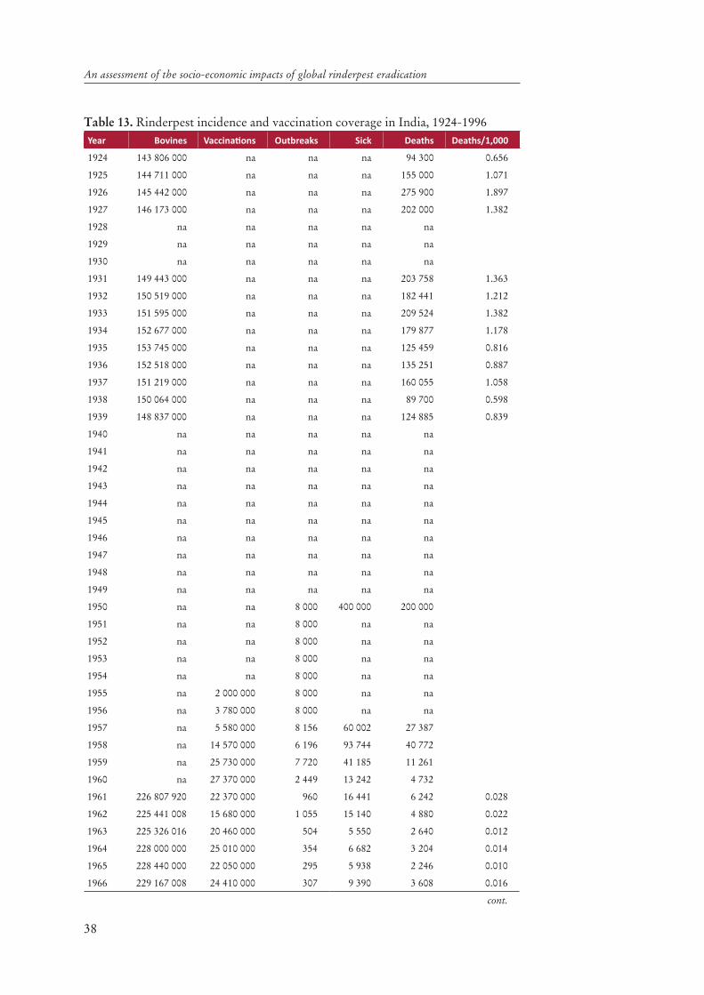
38

An assessment of the socio-economic impacts of global rinderpest eradication

Table 13. Rinderpest incidence and vaccination coverage in India, 1924-1996

1924 143 806 000 na na na 94 300 0.656

1925 144 711 000 na na na 155 000 1.071

1926 145 442 000 na na na 275 900 1.897

1927 146 173 000 na na na 202 000 1.382

1928 na na na na na

1929 na na na na na

1930 na na na na na

1931 149 443 000 na na na 203 758 1.363

1932 150 519 000 na na na 182 441 1.212

1933 151 595 000 na na na 209 524 1.382

1934 152 677 000 na na na 179 877 1.178

1935 153 745 000 na na na 125 459 0.816

1936 152 518 000 na na na 135 251 0.887

1937 151 219 000 na na na 160 055 1.058

1938 150 064 000 na na na 89 700 0.598

1939 148 837 000 na na na 124 885 0.839

1940 na na na na na

1941 na na na na na

1942 na na na na na

1943 na na na na na

1944 na na na na na

1945 na na na na na

1946 na na na na na

1947 na na na na na

1948 na na na na na

1949 na na na na na

1950 na na 8 000 400 000 200 000

1951 na na 8 000 na na

1952 na na 8 000 na na

1953 na na 8 000 na na

1954 na na 8 000 na na

1955 na 2 000 000 8 000 na na

1956 na 3 780 000 8 000 na na

1957 na 5 580 000 8 156 60 002 27 387

1958 na 14 570 000 6 196 93 744 40 772

1959 na 25 730 000 7 720 41 185 11 261

1960 na 27 370 000 2 449 13 242 4 732

1961 226 807 920 22 370 000 960 16 441 6 242 0.028

1962 225 441 008 15 680 000 1 055 15 140 4 880 0.022

1963 225 326 016 20 460 000 504 5 550 2 640 0.012

1964 228 000 000 25 010 000 354 6 682 3 204 0.014

1965 228 440 000 22 050 000 295 5 938 2 246 0.010

1966 229 167 008 24 410 000 307 9 390 3 608 0.016

cont.

39

1967 230 240 000 25 900 000 577 10 833 5 835 0.025

1968 231 340 016 26 030 000 870 7 185 2 487 0.011

1969 232 450 000 29 610 000 396 7 267 2 723 0.012

1970 233 560 000 33 190 000 374 6 140 2 571 0.011

1971 234 690 000 34 450 000 360 8 986 2 153 0.009

1972 235 810 000 44 200 000 207 2 710 1 532 0.006

1973 236 980 016 47 260 000 160 3 572 1 528 0.006

1974 238 140 000 44 090 000 195 3 342 1 627 0.007

1975 239 377 008 43 220 000 160 2 814 1 433 0.006

1976 241 280 000 51 550 000 161 4 314 2 630 0.011

1977 242 315 008 59 430 000 140 4 768 2 947 0.012

1978 245 322 000 50 970 000 143 2 662 1 146 0.005

1979 248 980 000 55 000 000 121 0 0 0.000

1980 252 570 000 56 600 000 183 0 0 0.000

1981 256 200 000 56 600 000 213 0 0 0.000

1982 262 237 008 56 600 000 127 2 295 691 0.003

1983 265 370 016 56 600 000 82 0 0 0.000

1984 268 550 000 56 600 000 121 0 0 0.000

1985 271 770 000 65 200 000 117 0 0 0.000

1986 275 050 016 65 200 000 175 na 2 503 0.009

1987 275 662 008 65 200 000 232 na 3 318 0.012

1988 278 120 000 65 200 000 321 na 4 590 0.017

1989 280 600 000 65 200 000 155 na 2 217 0.008

1990 283 070 000 na 126 na 1 802 0.006

1991 285 660 000 na 94 na 1 344 0.005

1992 288 790 000 na 96 na 1 373 0.005

1993 288 952 000 na 103 na 1 473 0.005

1994 289 128 000 na 29 na 415 0.001

1995 289 319 000 na 10 na 143 0.000

1996 289 525 000 na 0 0 0 0.000

Source: Compiled from data in Khera (1979); Nair (1991); and FAOSTAT.

earliest period in which complete production and price data were available from local and international sources (IMF, FAOSTAT). For this case, we assume that under limited vaccination, 10 075 million vaccinations were administered, equivalent to the average quantity used during the late 1950s before NPRE started in earnest. We further assumed an additional mortality rate associated with rinderpest of 0.0152 percent and morbidity rate of 0.0343 percent based on the 1957-58 average.

2. A mass vaccination vs. “no control” scenario: In this scenario, our counter-factual case is akin to the situation pre-independence in which mortality rates were much higher (0.1 percent per annum), as were morbidity rates (0.26 per-cent), based on averages prevailing in the 1920s-1940s. We further assume that vaccination coverage was limited to just 2 million doses per year.

A new methodological framework for the ex-post assessment of rinderpest eradication

Table 13. Cont.d

40

An assessment of the socio-economic impacts of global rinderpest eradication

3. Market access scenario, post-NPRE: The final scenario looked at the impact of NPRE on market access from the 1990s onward. In this case, we consid-ered the period 1992-2007 and examined how trade effects with and without rinderpest control influenced its viability as a policy intervention. We assumed mortality and morbidity rates in the counterfactual as those prevailing in the 1980s and looked only at the additional costs associated with the final push in the 1990s to eradicate the disease. On the trade side, the counterfactual assumes that export growth was at 1980-89 average levels for buffalo meat (1.92 percent per annum) and 1990-91 average levels for cattle meat (2.16 per-cent per annum). The 1990-91 rates were used for cattle meat because exports during the 1980s were relatively small and difficult to associate with a defined trend until the end of the 1980s.

ratio of mass vaccination vis-à-vis limited vaccination was slightly less than 1 (0.98), suggesting that the mass vaccination programme of the 1970s and 1980s, compared to more limited programmes earlier, may not, prima facie, been a good investment. In particular, the high additional costs of vaccination initially dwarf relatively lim-

rinderpest control (Figure 9). A couple of caveats temper the conclusion of this analysis, however. First, the cumulative impact of rinderpest control eventually outweighs the added costs, as Figure 9 illustrates, around 1980. A longer-term time perspective would likely increase the BCR in this scenario. Second, the analysis does not consider the multiplier impacts on other, non-livestock parts of the econ-omy. While a SAM for India was not available for this analysis, Roeder and Rich (2009) estimated multipliers for the livestock sector in Africa and South Asia that

noted in the sensitivity analysis discussed below, the BCR is highly sensitive to the assumption of mortality rates associated with rinderpest.

vaccination programme becomes much higher (estimated at 5.42), with positive and -

pends on the assumed mortality rate associated with rinderpest. Figure 11 illustrates the results of sensitivity analysis in which the mortality rate associated with rinder-pest was varied between 0.01 percent and 0.1 percent. The analysis demonstrates much higher BCRs as rinderpest-attributable mortality rises.

Table 14. Control Scenarios

1) Limited vaccination during 1972-1989: annual vaccination of 10.075 million herds, mortality/moribidity rates of late 1950s

0.98

2) “No control” during 1972-1989: annual vac-cination of 2 million herds; mortality/morbidity rates of 1920s-1940s

5.42

3) No eradication in 1990s: control patterns and market access for bovine meat based on 1980s

64.77

Source: Simulations with DynMod

41

the NPRE, we observe a huge success from the standpoint of its BCR (well over 64, see Table 14). The large size of this BCR is fueled by much higher market access (a more than six-fold increase in volume terms) for livestock exports that boomed as rinderpest freedom was achieved (Figure 12).

To assess rinderpest control in an economywide framework, we developed a new Social Accounting Matrix (SAM) for India, updating detailed industry accounts and

(see Table 15). The resulting table supports the same multiplier estimation and de-composition analysis carried out for Chad. These results are interesting in their own right and for comparison. One valuable property of the Indian input-output data is an activity account for Animal Services, which are primarily comprised of animal traction. This account was included in the Indian SAM for reasons that should be more widely recognized, especially in Asia and Africa. Although meat consump-tion at the village level is limited (particularly in India), the services of animal trac-tion are part of the bedrock of local economic activity, not only in farm production but in commercial distribution and other transport services. Moreover, this service would be quite sensitive to bovine health status, and as such offers an important assessment metric for rinderpest damages. As can be seen in Table 16, multipli-ers from Animal Services are large and widely dispersed across stakeholders in the

agrofood supply chain and that supply chain’s pervasive linkages across the Indian economy. Table 17 provides more focused results, showing only the household income multipliers arising from livestock activities. It is noteworthy that animal services have the largest impact across this category of agriculture, both for house-holds generally and across the Indian economy. These results contrast sharply with a long literature on valuing animal traction (e.g. Binswanger et al., 1982). We be-

Figure 9. vaccination in India, 1972-1989.

Source: Model simulations with DynMod.

A new methodological framework for the ex-post assessment of rinderpest eradication

42

An assessment of the socio-economic impacts of global rinderpest eradication

Figure 10. control in India, 1972-1989.

Source: Model simulations with DynMod.

Figure 11. different mortality rates.

Source: Model simulations with DynMod.

43

lieve those studies to be biased downward because of their emphasis on valuing the animals (as capital goods) rather than valuation of their services. Even those studies

-vice income to animals will understate their contribution to economywide income.

The next step with the Indian SAM is to decompose household income effects that originate from livestock, their products, and services. Because the Indian SAM details income by locality and employment status, we can better understand the pervasive nature of livestock’s contribution to domestic livelihoods. Table 18 de-tails the path decomposition of each livestock activity on each household group. There are many details here, but a few salient aspects deserve emphasis. As would be expected, rural households gain most from livestock activities, with the poorest (labourer households) gaining more than rural enterprise households. These pro-rural and pro-poor effects reveal the important of smallholder livestock to national livelihood promotion. As the livestock and livestock products sectors continue modernization, it is essential that supporting rural policies work to sustain this source of income for rural poor majorities.

Closer inspection of the decomposition results shows the potency of market ac-cess in the livestock-livelihood pathway. For every household type, the second-ary agent in income effects from the cattle/milk sector (AMLK) is food processing (APFD), an activity that requires market access and (for many poor in India) the animal services to achieve this. For all rural households and a few (low income) urban ones, we also see the second largest source of livestock generated income is income attributed to animal (traction) services in rice production.

To place livestock and animal health assessment in a long-term context, we now follow the example of the Chad assessment and apply a dynamic CGE forecasting tool to our data for India. The macroeconomic impacts of the same two scenarios (falling livestock productivity and export disruption) are summarized in Table 19 and

Figure 12. Changes in bovine meat exports associated with rinderpest control and “no control” scenario, 1992-2007.

Source: Model simulations with DynMod.

A new methodological framework for the ex-post assessment of rinderpest eradication

44

An assessment of the socio-economic impacts of global rinderpest eradication

1 Paddy Rice CPAD

2 Wheat CWHT

Cereals,Grains etc,Other crops

CCER

4 Sugar Cane CSGR

Oilseeds COSD

Cash crops CCAS

Cattle Meat and Milk CMLK

8 AnimalServ CANS

9 PoultryEgg CPOL

OthLvstk CLVS

11 Forestry CFRS

12 Fishing CFSH

Coal CCOL

14 Petroleum COIL

Gas Manufacture & Distri-bution

CGAS

Food & beverages CPFD

Animal Textiles CATX

18 Other Textiles COTX

19 Apparel CAPR

Leather CLEA

21 Wood CLUM

22 Mineral Products CNMM

ProductsCPET

24 Chemicals CCRP

AgroChem CACH

Pharma and Cosmetics CPCH

Paper & Paper prod. CPPP

28 IronSteel CI_S

29 NonFerMetals CNFM

Cement CCEM

Aluminium CALU

Other manufacturing COMF

Machinery COME

Electronic Machinery CELC

Cars and Trucks CMVH

Bikes and Cycles CBVH

Aircraft CAVH

Rail Vehicles CRVH

Ships CWVH

Conventional Electric Power CELE

41 Water CWAT

42 Construction CCON

Road Vehicle Transport CVTP

44 Rail Transport CRTP

Air Transport CATP

Water Transport CWTP

Health & medical CHLM

48 Communication CCOM

49 Trade CTRD

All other services CSER

Skilled Labor LABSK

Capital CAP

Land LAN

Rural Nonag Self Employed RNagSE

Rural Ag Laborers RAgLab

Rural Other Laborers ROthLab

Rural Ag Self Employed RAgSE

Rural Other Households ROthHH

Urban Self Employed USE

Urban Salaried Workers USal

Urban Casual Labor UCasLab

Urban Other Households UOthHH

Private Enterprises PvtEnt

Public Enterprises PubEnt

Government GOV

Indirect Taxes ITX

Trade Taxes TTX

Direct Taxes DTX

Capital Account CAC

Rest of World ROW

Table 15. Institutions of the 2008 India SAM

45

Tab

le 1

6. A

gric

ultu

ral a

ctiv

ity

mul

tipl

iers

for

the

Indi

a SA

MAW

HT

ACE

RA

SGR

AO

SDA

CAS

AA

NS

ALV

S

Pad

dy R

ice

1.49

0.11

0.09

0.10

0.08

0.11

0.07

0.09

0.12

0.08

Whe

at

0.06

1.61

0.07

0.06

0.05

0.08

0.05

0.07

0.04

0.05

Cer

eals

,Gra

ins

etc,

Oth

er c

rops

0.

050.

071.

200.

050.

040.

050.

040.

060.

100.

05Su

gar

Can

e0.

020.

020.

021.

210.

020.

020.

020.

020.

010.

02O

ilsee

ds0.

030.

040.

030.

031.

090.

030.

030.

030.

030.

03C

ash

crop

s 0.

190.

200.

210.

190.

191.

230.

220.

670.

140.

36C

attl

e M

eat a

nd M

ilk0.

080.

100.

080.

090.

080.

091.

070.

080.

070.

07A

nim

alSe

rv0.

070.

040.

120.

040.

080.

040.

011.

030.

020.

02P

oult

ryE

gg0.

010.

010.

010.

010.

010.

010.

010.

011.

010.

01O

thL

vstk

0.04

0.03

0.04

0.03

0.04

0.03

0.02

0.02

0.02

1.02

For

estr

y0.

020.

020.

020.

020.

020.

020.

020.

020.

020.

02F

ishi

ng

0.02

0.03

0.02

0.02

0.02

0.02

0.02

0.02

0.02

0.02

Coa

l 0.

020.

020.

010.

020.

010.

010.

010.

010.

010.

01P

etro

leum

0.10

0.11

0.08

0.08

0.07

0.07

0.05

0.07

0.05

0.06

Gas

Man

ufac

ture

& D

ist

0.01

0.02

0.01

0.01

0.01

0.01

0.00

0.01

0.00

0.00

Foo

d &

bev

erag

es

0.19

0.22

0.18

0.21

0.18

0.19

0.17

0.24

0.18

0.19

Ani

mal

Tex

tile

s0.

000.

010.

000.

000.

000.

000.

000.

000.

000.

00O

ther

Tex

tile

s0.

060.

070.

050.

060.

050.

060.

050.

050.

050.

05A

ppar

el0.

030.

040.

030.

040.

030.

030.

030.

030.

030.

03L

eath

er0.

010.

010.

010.

010.

010.

010.

010.

010.

010.

01W

ood

0.01

0.01

0.01

0.01

0.01

0.01

0.01

0.01

0.01

0.01

Min

eral

Pro

duct

s0.

010.

010.

010.

010.

010.

010.

000.

000.

000.

000.

170.

190.

150.

150.

140.

130.

090.

130.

090.

11C

hem

ical

s0.

120.

140.

090.

110.

100.

090.

070.

090.

070.

08A

groC

hem

0.15

0.20

0.09

0.13

0.10

0.09

0.03

0.06

0.03

0.04

Pha

rma

and

Cos

met

ics

0.04

0.04

0.03

0.04

0.04

0.04

0.03

0.03

0.03

0.03

Pap

er &

Pap

er p

rod.

0.

030.

030.

020.

030.

020.

020.

020.

030.

020.

02Ir

onSt

eel

0.02

0.02

0.02

0.02

0.02

0.02

0.01

0.02

0.01

0.01

Non

Fer

Met

als

0.00

0.00

0.00

0.00

0.00

0.00

0.00

0.00

0.00

0.00

Cem

ent

0.01

0.01

0.01

0.00

0.00

0.00

0.00

0.00

0.00

0.00

Alu

min

ium

0.01

0.01

0.01

0.01

0.01

0.01

0.01

0.01

0.01

0.01

Oth

er m

anuf

actu

ring

0.

040.

050.

040.

040.

040.

040.

030.

040.

030.

03M

achi

nery

0.

020.

030.

030.

020.

020.

020.

010.

020.

020.

02E

lect

roni

c M

achi

nery

0.04

0.04

0.03

0.04

0.03

0.03

0.03

0.03

0.03

0.03

cont

.

A new methodological framework for the ex-post assessment of rinderpest eradication

46

An assessment of the socio-economic impacts of global rinderpest eradication

AWH

TA

CER

ASG

RA

OSD

ACA

SA

AN

SA

LVS

Ship

s0.

000.

000.

000.

000.

000.

000.

000.

000.

000.

00C

onve

ntio

nal E

lect

ric

Pow

er0.

120.

140.

070.

090.

070.

070.

050.

070.

050.

05W

ater

0.

000.

000.

000.

000.

000.

000.

000.

000.

000.

00C

onst

ruct

ion

0.04

0.05

0.03

0.03

0.03

0.03

0.02

0.03

0.02

0.02

Roa

d V

ehic

le T

rans

port

0.22

0.25

0.20

0.22

0.19

0.19

0.16

0.25

0.15

0.19

Car

s an

d T

ruck

s0.

020.

020.

010.

020.

010.

010.

010.

020.

010.

01B

ikes

and

Cyc

les

0.01

0.01

0.01

0.01

0.01

0.01

0.01

0.01

0.01

0.01

Air

craf

t0.

000.

000.

000.

000.

000.

000.

000.

000.

000.

00R

ail V

ehic

les

0.01

0.01

0.00

0.00

0.00

0.00

0.00

0.00

0.00

0.00

Rai

l Tra

nspo

rt

0.03

0.04

0.02

0.03

0.02

0.02

0.02

0.02

0.02

0.02

Air

Tra

nspo

rt

0.01

0.01

0.01

0.01

0.01

0.01

0.01

0.01

0.00

0.01

Wat

er T

rans

port

0.01

0.01

0.01

0.01

0.01

0.01

0.01

0.01

0.01

0.01

Hea

lth

& m

edic

al

0.05

0.05

0.04

0.05

0.04

0.05

0.04

0.04

0.04

0.04

Com

mun

icat

ion

0.03

0.03

0.03

0.03

0.03

0.03

0.02

0.03

0.02

0.02

Tra

de0.

330.

380.

300.

290.

270.

260.

260.

570.

220.

36A

ll ot

her

serv

ices

0.

440.

500.

390.

470.

400.

410.

350.

410.

340.

36T

otal

for

Act

ivit

ies

4.48

5.09

3.92

4.13

3.73

3.70

3.21

4.48

3.17

3.58

Skill

ed L

abor

1.14

1.33

1.06

1.27

1.10

1.15

1.05

1.03

1.06

1.03

Cap

ital

0.72

0.84

0.62

0.71

0.62

0.62

0.82

0.72

0.83

0.78

Lan

d0.

340.

400.

340.

440.

380.

410.

100.

240.

100.

15T

otal

for

Fact

ors

2.20

2.58

2.03

2.42

2.10

2.19

1.98

1.99

1.98

1.95

Rur

al N

onag

Sel

f Em

ploy

ed0.

150.

170.

140.

160.

140.

140.

150.

140.

150.

14R

ural

Ag

Lab

orer

s0.

180.

210.

170.

200.

180.

180.

170.

160.

170.

16R

ural

Oth

er L

abor

ers

0.06

0.07

0.05

0.07

0.06

0.06

0.06

0.05

0.06

0.05

Rur

al A

g Se

lf E

mpl

oyed

0.64

0.75

0.61

0.75

0.65

0.69

0.41

0.52

0.40

0.44

Rur

al O

ther

Hou

seho

lds

0.12

0.14

0.11

0.12

0.11

0.11

0.13

0.12

0.13

0.12

Urb

an S

elf E

mpl

oyed

0.21

0.24

0.19

0.22

0.19

0.19

0.21

0.19

0.21

0.20

Urb

an S

alar

ied

Wor

kers

0.44

0.51

0.40

0.48

0.42

0.44

0.41

0.39

0.41

0.40

Urb

an C

asua

l Lab

or0.

070.

080.

060.

070.

060.

070.

060.

060.

060.

06U

rban

Oth

er H

ouse

hold

s0.

040.

050.

040.

050.

040.

040.

050.

040.

050.

04T

otal

for

Hou

seho

lds

1.90

2.22

1.77

2.12

1.84

1.92

1.64

1.69

1.64

1.63

Gra

nd T

otal

8.59

9.89

7.72

8.67

7.67

7.81

6.83

8.15

6.79

7.17

Tab

le 1

6. C

ont.d

47

Table 17. Household livestock multipliersAANS ALVS

Rural Nonag Self Employed 0.15 0.14 0.15 0.14

Rural Ag Labourers 0.17 0.16 0.17 0.16

Rural Other Labourers 0.06 0.05 0.06 0.05

Rural Ag Self Employed 0.41 0.52 0.40 0.44

Rural Other Households 0.13 0.12 0.13 0.12

Urban Self Employed 0.21 0.19 0.21 0.20

Urban Salaried Workers 0.41 0.39 0.41 0.40

Urban Casual Labourers 0.06 0.06 0.06 0.06

Urban Other Households 0.05 0.04 0.05 0.04

Total for Households 1.64 1.69 1.64 1.63

Grand Total 6.83 8.15 6.79 7.17

RNagSE AMLK 0.079 0.036 1.143 0.041 52 52

RNagSE APFD AMLK 0.004 1.414 0.005 6 59

RNagSE ACAS LAN RAgSE AMLK 0.001 1.585 0.001 1 60

RNagSE APAD AANS 0.014 0.001 1.624 0.002 15 15

RNagSE ACER AANS 0.001 1.312 0.002 14 28

RNagSE ACAS AANS 0.001 1.314 0.002 12 40

RNagSE APOL 0.010 0.004 1.085 0.005 48 48

RNagSE ALVS 0.022 0.008 1.098 0.009 40 40

RNagSE APFD ALVS 0.001 1.370 0.001 4 44

RAgLab AMLK 0.114 0.044 1.203 0.053 47 47

RAgLab APFD AMLK 0.006 1.471 0.009 8 55

RAgLab ACAS LAN RAgSE AMLK 0.001 1.631 0.002 2 57

RAgLab ASER LABSK USal AMLK 0.001 1.934 0.001 1 57

RAgLab APAD AANS 0.024 0.002 1.702 0.004 17 17

RAgLab ACER AANS 0.003 1.381 0.004 15 33

RAgLab AOSD AANS 0.001 1.266 0.001 4 37

RAgLab ACAS AANS 0.002 1.364 0.003 14 51

RAgLab APFD AOSD AANS 0.001 1.542 0.001 4 55

RAgLab APOL 0.014 0.005 1.148 0.006 43 43

RAgLab ASER APOL 0.001 1.532 0.001 6 49

RAgLab ALVS 0.033 0.010 1.160 0.012 35 35

RAgLab APAD ALVS 0.001 1.692 0.001 4 39

RAgLab APFD ALVS 0.001 1.428 0.001 4 43

RAgLab ALEA ALVS 0.001 1.408 0.001 2 46

ROthLab AMLK 0.120 0.052 1.114 0.057 48 48

ROthLab APFD AMLK 0.006 1.386 0.008 7 55

ROthLab ASER AMLK 0.001 1.513 0.001 1 55

ROthLab ACAS LAN RAgSE AMLK 0.001 1.556 0.002 1 57

ROthLab ASER LABSK USal AMLK 0.001 1.935 0.001 1 58

ROthLab ASER CAP RAgSE AMLK 0.001 1.857 0.001 1 59

ROthLab APAD AANS 0.021 0.002 1.581 0.003 14 14

ROthLab ACER AANS 0.002 1.276 0.003 13 27

ROthLab AOSD AANS 0.001 1.169 0.001 3 30

cont.

Table 18. Path decomposition for households in India

A new methodological framework for the ex-post assessment of rinderpest eradication

48

An assessment of the socio-economic impacts of global rinderpest eradication

ROthLab ACAS AANS 0.002 1.283 0.002 11 42

ROthLab APFD AOSD AANS 0.001 1.448 0.001 4 46

ROthLab APOL 0.015 0.006 1.054 0.006 44 44

ROthLab ASER APOL 0.001 1.447 0.001 6 50

ROthLab ALVS 0.034 0.012 1.067 0.012 36 36

ROthLab APAD ALVS 0.001 1.574 0.001 3 39

ROthLab APFD ALVS 0.001 1.339 0.001 4 43

ROthLab ALEA ALVS 0.001 1.296 0.001 2 45

RAgSE AMLK 0.095 0.045 1.336 0.060 63 63

RAgSE APFD AMLK 0.004 1.599 0.006 6 70

RAgSE APAD AANS 0.015 0.001 1.881 0.002 16 16

RAgSE ACER AANS 0.001 1.536 0.002 14 31

RAgSE ACAS AANS 0.001 1.470 0.002 13 43

RAgSE APOL 0.012 0.005 1.289 0.007 59 59

RAgSE ALVS 0.027 0.010 1.299 0.013 50 50

RAgSE APFD ALVS 0.001 1.563 0.001 4 53

ROthHH AMLK 0.087 0.039 1.143 0.045 52 52

ROthHH APFD AMLK 0.004 1.416 0.005 6 57

ROthHH ACAS LAN RAgSE AMLK 0.001 1.590 0.001 1 58

ROthHH ASER LABSK USal AMLK 0.001 1.968 0.001 1 60

ROthHH ASER CAP RAgSE AMLK 0.001 1.840 0.001 1 61

ROthHH APAD AANS 0.014 0.001 1.627 0.002 12 12

ROthHH ACER AANS 0.001 1.313 0.002 13 24

ROthHH ACAS AANS 0.001 1.319 0.001 10 34

ROthHH APOL 0.011 0.005 1.085 0.005 47 47

ROthHH ASER APOL 0.001 1.465 0.001 7 54

ROthHH ALVS 0.024 0.009 1.098 0.010 40 40

ROthHH APFD ALVS 0.001 1.371 0.001 3 43

USE AMLK 0.088 0.042 1.183 0.049 56 56

USE APFD AMLK 0.003 1.457 0.005 5 62

USE ASER AMLK 0.001 1.556 0.001 1 62

USE ASER LABSK USal AMLK 0.001 1.970 0.001 1 64

USE ASER CAP RAgSE AMLK 0.001 1.865 0.001 1 65

USE APAD AANS 0.012 0.001 1.687 0.001 11 11

USE ACER AANS 0.001 1.363 0.002 14 24

USE ACAS AANS 0.001 1.363 0.001 9 33

USE APOL 0.011 0.005 1.128 0.006 51 51

USE ASER APOL 0.001 1.496 0.001 8 59

USE ALVS 0.024 0.009 1.141 0.011 44 44

USE APFD ALVS 0.001 1.415 0.001 3 47

USal AMLK 0.068 0.028 1.262 0.035 52 52

USal APFD AMLK 0.002 1.541 0.003 5 57

USal ASER AMLK 0.001 1.606 0.001 1 58

USal ASER CAP RAgSE AMLK 0.001 1.945 0.001 2 60

USal ACER AANS 0.010 0.001 1.457 0.001 12 12

USal APOL 0.009 0.003 1.210 0.004 46 46

USal ASER APOL 0.001 1.549 0.001 12 57

cont.

Table 18. Cont.d

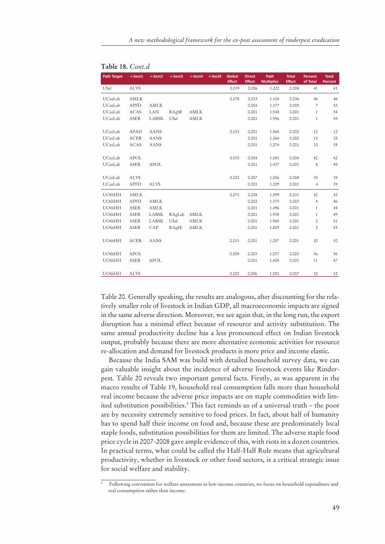
49

A new methodological framework for the ex-post assessment of rinderpest eradication

USal ALVS 0.019 0.006 1.222 0.008 41 41

UCasLab AMLK 0.078 0.033 1.104 0.036 46 46

UCasLab APFD AMLK 0.004 1.377 0.005 7 53

UCasLab ACAS LAN RAgSE AMLK 0.001 1.548 0.001 1 54

UCasLab ASER LABSK USal AMLK 0.001 1.936 0.001 1 55

UCasLab APAD AANS 0.013 0.001 1.568 0.002 12 12

UCasLab ACER AANS 0.001 1.264 0.002 13 25

UCasLab ACAS AANS 0.001 1.274 0.001 10 35

UCasLab APOL 0.010 0.004 1.043 0.004 42 42

UCasLab ASER APOL 0.001 1.437 0.001 8 49

UCasLab ALVS 0.022 0.007 1.056 0.008 35 35

UCasLab APFD ALVS 0.001 1.329 0.001 4 39

UOthHH AMLK 0.073 0.028 1.099 0.031 42 42

UOthHH APFD AMLK 0.002 1.373 0.003 4 46

UOthHH ASER AMLK 0.001 1.496 0.001 1 48

UOthHH ASER LABSK RAgLab AMLK 0.001 1.938 0.001 1 49

UOthHH ASER LABSK USal AMLK 0.001 1.945 0.001 2 51

UOthHH ASER CAP RAgSE AMLK 0.001 1.829 0.001 2 53

UOthHH ACER AANS 0.011 0.001 1.257 0.001 10 10

UOthHH APOL 0.009 0.003 1.037 0.003 36 36

UOthHH ASER APOL 0.001 1.428 0.001 11 47

UOthHH ALVS 0.020 0.006 1.050 0.007 32 32

Table 18. Cont.d

Table 20. Generally speaking, the results are analogous, after discounting for the rela-tively smaller role of livestock in Indian GDP, all macroeconomic impacts are signed in the same adverse direction. Moreover, we see again that, in the long run, the export disruption has a minimal effect because of resource and activity substitution. The same annual productivity decline has a less pronounced effect on Indian livestock output, probably because there are more alternative economic activities for resource re-allocation and demand for livestock products is more price and income elastic.

Because the India SAM was build with detailed household survey data, we can gain valuable insight about the incidence of adverse livestock events like Rinder-pest. Table 20 reveals two important general facts. Firstly, as was apparent in the macro results of Table 19, household real consumption falls more than household real income because the adverse price impacts are on staple commodities with lim-ited substitution possibilities.3 This fact reminds us of a universal truth – the poor are by necessity extremely sensitive to food prices. In fact, about half of humanity has to spend half their income on food and, because these are predominately local staple foods, substitution possibilities for them are limited. The adverse staple food price cycle in 2007-2008 gave ample evidence of this, with riots in a dozen countries. In practical terms, what could be called the Half-Half Rule means that agricultural productivity, whether in livestock or other food sectors, is a critical strategic issue for social welfare and stability.

3 Following convention for welfare assessment in low-income countries, we focus on household expenditure and real consumption rather than income.

50

An assessment of the socio-economic impacts of global rinderpest eradication

Table 19. Macroeconomic impacts of livestock sector scenarios for India(Percent change from baseline values in 2030)

Real GDP -6% -7%HH Income -3% -3%Consumption -8% -8%Exports -5% -5%Imports -5% -6%OutputPaddy Rice -1% -1%Wheat -2% -2%Cereals, Grains etc. -1% -1%Sugar Cane -3% -3%Oilseeds -2% -2%Cash crops -2% -2%Milk -34% -34%Animal Services -2% -2%Poultry&Eggs -3% -4%Other Livestock -21% -22%Forestry -4% -4%Fishing -4% -4%Coal -4% -4%Petroleum -5% -5%Gas Manufacture & Distribution -4% -4%Food & beverages -3% -3%Animal Textiles -8% -8%Other Textiles -1% -1%Apparel -2% -2%Leather -19% -20%Wood -4% -4%Mineral Products -2% -2%

-4% -4%Chemicals -3% -3%Agro Chemicals -2% -2%Pharma and Cosmetics -4% -4%Paper & Paper prod. -4% -4%Iron&Steel -4% -4%NonFerrous Metals -5% -5%Cement -4% -4%Aluminum -5% -5%Other manufacturing -4% -4%Machinery -4% -4%Electronic Machinery -4% -4%Cars and Trucks -4% -4%Bikes and Cycles -4% -4%Aircraft -5% -5%Rail Vehicles -4% -4%Conventional Electric Power -4% -4%Water -3% -3%Construction -4% -4%Road Vehicle Transport -4% -4%Rail Transport -4% -4%Air Transport -5% -5%Water Transport -5% -5%Health & medical -4% -4%Communication -4% -4%Trade -5% -5%All other services -4% -4%

51

The second general insight from Table 20 is heterogeneity. Clearly, adverse live-stock production events affect different households differently. Most importantly for the present research, it is apparent that low-income households suffer much more in relative terms. Rural Agricultural Labourers, the poorest, suffer three times as much of a decline in real consumption. This effect arises for two reasons, one on the expenditure side and one on the income side. Food prices rise because of higher marginal cost in livestock production, and they most adversely affect real consump-tion by the poorest households for reasons just discussed. Second, falling livestock productivity translates into lower productivity for those whose livelihoods most depend (in share of income terms) on animals and animal services, again the poor-est farm households. All in all, the results for India drive home a simple message, livestock is integral to the lives and future economic opportunities of the country’s poor majority, and promoting growth and value creation in smallholder livestock can be a potent catalyst for poverty reduction.Summary of results

but the message of the present exercise is likely to remain the same. Livestock is an essential contributor to poor people’s food security and livelihoods, especially in rural areas where the majority of global poverty persists. For this reason, sustained initiative to reduce the incidence and persistence of animal diseases is an essential component of global development policy, supporting vital capacity for the poor to advance their own circumstances.

In this study, we present two case studies of very different developing econo-mies. Despite their differences, however, the implication of these results is clear. As long as smallholders, embedded in or in transit from subsistence, make up the ma-jority of the rural population, and extensive poverty persists there, animal products and services will be essential to national livelihood. Moreover, those products and services support a wide array of commercial linkages between the rural poor and the rest of the economy that would be absent without the animals. Rinderpest and other bovine diseases pose a direct threat to this extensive web of economic activity, and to its capacity for facilitating market access and self-directed poverty reduction.

Endemic high-impact animal diseases like rinderpest; even if they don’t induce human illness, represent major economic threats to countries with limited house-

Table 20. Household real consumption effects

Rural Nonag Self Employed -3% -3%

Rural Ag Labourers -15% -15%

Rural Other Labourers -5% -5%

Rural Ag Self Employed -5% -5%

Rural Other Households -4% -4%

Urban Self Employed -9% -10%

Urban Salaried Workers -5% -5%

Urban Casual Labourers -4% -5%

Urban Other Households -6% -6%

A new methodological framework for the ex-post assessment of rinderpest eradication

52

An assessment of the socio-economic impacts of global rinderpest eradication

For low-income countries, a few percentage points of GDP can make the differ-ence between meeting basic needs and large-scale human misery. Even in simple accounting terms, this amount is enough to justify large defensive investments in integrated livestock health maintenance. Although Rinderpest represents an even-tual victory, our empirical results suggest that recurrent investment levels are prob-ably too small.

53

The approach outlined in this paper has provided a method to assess in a relatively

Clearly, the analysis is incomplete, and indeed in the case of rinderpest, beset by an extreme lack of data on both economic parameters (prices, trade, etc.) and costs associated with rinderpest control and eradication. Nonetheless, the methodolo-gy attempts to address the key dimensions of disease eradication as a guideline to measure future eradication impacts and as a template to organize the collection of appropriate necessary for improved monitoring and evaluation of current disease control and eradication efforts (e.g., PPR, FMD, etc.).

An important consideration in the rinderpest eradication story is that local con-text matters, and some aspects of control (and different levels of analysis) will be more or less important in different settings. In West Africa, the higher propor-

structures on the overall cost-effectiveness of rinderpest control. The incidence of drought complicates matters, and more work will be required to tease out rinderpest impacts from other mortality effects in the livestock production system. In other cases, population dynamics will likely matter less, with the contextual aspects of the eradication programme playing an important role. India is a case in point. Between 1960-1990, mortality due to rinderpest was usually under 5 000 animals per year in a production system of well over 250 million bovines, suggesting that production impacts of rinderpest control/eradication would be marginal at best. On the other hand, the revealed impact of rinderpest eradication since 1990 has been a massive increase in market access for buffalo meat in particular, as trading partners have ac-

these nuances, providing general guidance of the scope of impacts to consider, given the local setting and data available.

Blakeway, S. 1995. Evaluation of the UNICEF Operation Lifeline Sudan, southern sector livestock programme, Unicef - OLS, Nairobi.

Bullock, D., Garcia, P. & Lee, Y. 1996. Towards Producer Welfare Measures in a Dynamic, Stochastic Framework. Working paper, University of Illinois at Ur-bana-Champaign.

Catley, A., Leyland, T., & Bishop, S. 2005. Policies, Practice, and Participation in Complex Emergencies: The Case of Livestock Interventions in South Sudan. Case Study for the Agriculture and Development Economics Division of the Food and Agriculture Organization of the United Nations, Tufts University, Medford, MA (USA).

Chuta, E.J. 1990. Income impacts of tissue culture vaccine on the control of rinder-pest in Nigeria. World Review of Animal Production 25(3), 75-80.

Defourny, J. & Thorbecke, E. 1984. Structural Path Analysis and Multiplier De-composition within a Social Accounting Matrix Framework. Economic Journal 94 (373), 111-136.

Diao, X. 2010. Economywide Impact of Avian Flu in Ghana: A Dynamic CGE Model Analysis Africa/Indonesia Team Working Paper No. 15, Pro-poor HPAI risk reduction project, Washington, DC, available at http://www.hpai-research.net/docs/Working_papers/wp15_IFPRI.pdf

Ekboir J.M. 1999. Potential impact of foot-and-mouth disease in California: the role and contribution of animal health surveillance and monitoring services. Ag-ricultural Issues Center, Davis, CA, USA.

Fafchamps, M. & Gavian, S. 1995. The determinants of livestock prices in Niger. Journal of African Economies, 6 (2). pp. 255-295.

Felton, M.R. & Ellis, P.R. 1978. Studies on the control of rinderpest in Nigeria, Study No. 23, University of Reading, UK (Mimeo).

Garber, D.S. 2009. Oil, investment, and economic development: A detailed look at the advent of Chad’s oil sector. Ph.D. dissertation, Department of Agricultural and Applied Economics, University of Wisconsin-Madison.

Garner M.G. & Lack M.B. 1995. An evaluation of alternate control strategies for foot-and-mouth disease in Australia: a regional approach. Prev. vet. Med., 23 (1-2), 9-32.

Golan, E.H., Vogel, S.J., Frenzen, P.D. & Ralston, K.L. 2001. Tracing the costs

and critical control point program for meat and poultry. Agricultural Economic Report Number 791, Washington, D.C., U.S. Department of Agriculture, Eco-nomic Research Service.

Jost, C.C., Mariner, J.C., Roeder, P.L., Sawitiri, E. & Macgregor-Skinner, G.J. 2007. Participatory epidemiology in disease surveillance and research. Rev. sci. tech. Off. int. Epiz. 26(3), 537-549.

Just, R.E., Hueth, D.L. & Schmitz, A. 2004. The welfare economics of public pol-icy: A practical approach to project and policy evaluation. Edward Elgar, Chel-tenham, UK (Chs. 4 & 5).

55

References

Khera, S.S. 1979. Rinderpest eradication programme in India. Proceedings of the 2nd International Symposium on Veterinary Epidemiology and Economics.

Kobayashi, M. 2006. Poultry Value Chain Study: Consultant Report. Unpublished Paper, Food and Agriculture Organization of the United Nations, Rome, Italy.

Lepissier, H.E. 1971. General technical report on OAU/STRC Joint Campaign against Rinderpest in Central and West Africa 1961 - 1969. OAU/STRC PMB 2359, Lagos, Nigeria.

Lesnoff, M., Saley, M., Adamou, K. & N’Djaffa Ouaga, H. 2007. Enquête démo-graphique 2006 sur le cheptel domestique au Niger: sites du Fakara, de Gabi et de Zermou: Rapport préliminaire. Nairobi, CIRAD/ILRI.

Lesnoff, M., Saley, M., Adamou, K. & N’Djaffa Ouaga, H. 2007. 12MO: Une méthodologie rétrospective pour l’estimation des paramètres démographiques des cheptels de ruminants domestiques tropicaux. Nairobi, CIRAD/ILRI.

Mahul O. & Durand B. 2000. Simulated economic consequences of foot-and-mouth disease epidemics and their public control in France. Prev. vet. Med., 47 (1-2), 23-38.

2006. Present Status of Rinderpest Diseases in Pakistan, Journal of Veterinary Medicine B, 53, 26-28.

Miller, R.E. & Blair, P.D. 1985. Input-output analysis: Foundations and extensions. Engelwood Cliffs, NJ, USA, Prentice-Hall.

Minot, N. & Goletti, F. 1998. Export Liberalization and Household Welfare: The Case of Rice in Viet Nam. American Journal of Agricultural Economics 80 (4), 738–749.

Nair, R.P.N. 1991. Status of rinderpest in India. Mimeo.Nawathe, D.R. & Lamorde, A.G. 1984. Socio-economic impact of rinderpest in

Nigeria. OIE Rev. Sci. Tech. 3(3): 575-581.Normile, D. 2008. Driven to extinction. Science 319, 1606-1609. Oussiguere, A. 2010. Historique de la peste bovine au Tchad. Unpublished report,

Food and Agriculture Organization of the United Nations (Mimeo).Perry, B.D., Randolph, T.F., Ashley, S., Chimedza, R., Forman, T., Morrison,

J., Poulton, C., Sibanda, L., Stevens, C., Tebele, N. & Yngstrom, I. 2003. The impact and poverty reduction implications of foot and mouth disease control in southern Africa, with special reference to Zimbabwe. International Livestock Research Institute (ILRI), Nairobi, Kenya.

Reinert, K.A. & Roland-Holst, D. 1997. Social Accounting Matrices, In J.F. Fran-cois and K.A. Reinert (eds.), Applied Methods for Trade Policy Analysis, Cam-bridge: Cambridge University Press.

Rich, K.M., Winter-Nelson, A. & Miller, G.Y. 2005. Enhancing Economic Models for Analysis of Animal Disease, -ternational des Epizooties 24 (3), 847-856.

Rich, K.M. & Winter-Nelson, A. 2007. An Integrated Epidemiological-Economic Analysis of Foot and Mouth Disease: Applications to the Southern Cone of South America. American Journal of Agricultural Economics 89 (3): 682-697.

Rich, K.M. & Perry, B.D. 2011. The economic and poverty impacts of animal dis-eases in developing countries: new roles, new demands for economics and epide-miology, Preventive Veterinary Medicine 101 (3-4), 133-147.

56

An assessment of the socio-economic impacts of global rinderpest eradication

Rich, K.M. & Wanyioke, F. 2010. An assessment of the regional and national so-cio-economic impacts of the 2007 Rift Valley Fever outbreak in Kenya. Ameri-can Journal of Tropical Medicine and Hygiene 83 (Suppl 2), 52-57.

Roeder, P. & Rich, K.M. 2009. Conquering the Cattle Plague: The global effort to eradicate rinderpest. Chapter 16 in David J. Spielman and Rajul Pandya-Lorch, Eds., Millions Fed: Proven Successes in Agricultural Development (Washing-ton, DC: International Food Policy Research Institute), pp. 109-116. Available

Roland-Holst, D. & Otte, J. 2007. Livestock and livelihoods: Development goals and indicators applied to Senegal. African Journal of Agricultural Research 2(6), 240-251.

Rushton, J., Viscarra, R., Otte, J., McLeod, A. & Taylor, N. 2007. Animal health economics – where have we come from and where do we go next? CAB Re-views: Perspectives in Agriculture, Veterinary Science, Nutrition and Natural Resources 1, No. 031, 1-10

Rushton, J., Pinto, J. & Taylor, N.M. 2009. Linking value chain analysis with epi-demiological risk analysis to improve disease prevention and control interven-tions. Proceedings of the International Society for Veterinary Epidemiology and Economics 10-14 August 2009.

Sadoulet, E. & de Janvry, A. 1995 Quantitative Development Policy Analysis. Bal-timore, Johns Hopkins University Press.

Tambi, E.N., Maina, O.W., Mukhebi, A.W. & Randolph, T.F. 1999. Economic impact assessment of rinderpest control in Africa, OIE Rev. Sci. Tech. 18(2): 458-77.

Thorbecke, E. 1992. . OECD Development Centre, Paris.

ONLINE PUBLICATION SERIESFAO ANIMAL PRODUCTION AND HEALTH WORKING PAPER

1. The use of cash transfers in livestock emergencies and their incorporation into Livestock Emergency Guidelines and Standards (LEGS), 2011 (E) http://www.fao.org/docrep/014/i2256e/i2256e00.pdf

2. Mapping supply and demand for animal-source foods to 2030, 2011 (E) http://www.fao.org/docrep/014/i2425e/i2425e00.pdf

3. Notes on Livestock, Food Security and Gender Equity, 2011 (E) http://www.fao.org/docrep/014/i2426e/i2426e00.pdf

4. Wealth Index mapping in the Horn of Africa, 2011 (E) http://www.fao.org/docrep/014/i2427e/i2427e00.pdf

5. Evolution du secteur avicole en Tunisie, 2011 (F) http://www.fao.org/docrep/015/i2549f/i2549f.pdf

6. Status of animal nutrition research and development activities in Tajikistan, Kyrgyzstan and Azerbaijan, 2012 (E) http://www.fao.org/docrep/015/i2582e/i2582e00.pdf

7. An assessment of the socio-economic impacts of global rinderpest eradication – Methodological issues and applications to rinderpest control programmes in Chad and India, 2012 (A)

Availability: January 2012

E - EnglishF - French** In preparation

Find more publications athttp://www.fao.org/ag/againfo/resources/en/publications.html