Final Report for ECSE-4460

Control Systems Design

Adam Blot Morrigan McNamara

Lloyd Mebane Aryn Shapiro

May 4, 2005 Rensselaer Polytechnic Institute

Abstract The purpose of this final project report is to present how we developed our semester design project, a duck-hunt autonomous duck-hunter, D.A.D. D.A.D. was able to play Nintendo’s Duck Hunt video game, and was capable to conquer several levels in the game. With the use of a webcam, our program was able to obtain the coordinates of a target, move the Nintendo Zapper Gun, which is a light gun, which was mounted on a pan – tilt mechanism, and fire the light gun. The hardest portions of this project was to design two controllers for the system, one for the pan motor and one for the tilt motor, and to integrate the image processing into the overall project.

ii

Table of Contents Introduction 1 Friction Identification 4 System Modeling 6 Controller Design and Validation 9 Image Acquisition 15 Schedule 19 Costs 21 Bibliography 22 Team Member Contribution 23 Appendix A: gains.m 24 Appendix B: Fast Response Graph 26 Appendix C: Critical Response Graph 27 Appendix D: friction.m 28 Appendix E: find_duck2.m 29 Appendix F: time test.m and output time graph 31 Appendix G: mounting pictures 32 Appendix H: rlls.m 33 Appendix I: fire.m 34 Appendix J: return_angles.m 35 Appendix K: temp_2.m 36 Appendix L: temp2.jpg 38 Appendix M: dad_final.mdl 39

iii

List of Figures Figure 1: System Layout 1 Figure 2: SolidWorks System Model 3 Figure 3: Frictional Analysis 4 Figure 4: Representation of the Tilt/Pan Response to Voltage Sweep 5 Figure 5: Simulink Model of PE System for Parameter Estimation 7 Figure 6: PID Model for Pan and Tilt 9 Figure 7: D.A.D. Nonlinear Model for Simulation 10 Figure 8: Pan – Tilt Nonlinear Model Step Responses 10 Figure 9: Model Validation – Tracking Command 11 Figure 10: Model Validation Zoom 11 Figure 11: System Step Response 12 Figure 12: Simulink Implementation of SAC 13 Figure 13: Step Response for PID and PIS+SAC 13 Figure 14: Sinusoidal Tracking Response Over Two Periods 14 Figure 15: Implemented D.A.D. System Controller 14 Figure 16: Webcam Acquired Images 15 Figure 17: Acquired Image 16 Figure 18: Processed Image 16 Figure 19: Template Image 16 Figure 20: Unwanted Objects 16 Figure 21: Set of Sample Processed Images 17

iv

List of Tables TABLE 1: DESIGN SPECIFICATIONS 2 TABLE 2: FRICTIONAL COEFFICIENTS 5 TABLE 3: FRICTION IDENTIFICATION AND INERTIA RESULTS 8 TABLE 4: CONDITIONS FOR IMAGE DATA 17 TABLE 5: GANTT CHART OF SCHEDULE 20 TABLE 6: PROJECT COST BREAKDOWN 21

v

Introduction The goal of our project was to develop a targeting control system that is capable of aiming and firing the Nintendo Entertainment System zapper for the purposes of defeating the classic game “Duck Hunt”. The system is known as the Duck-Hunt Autonomous Duck-Hunter (D.A.D.) The zapper gun is mounted on a pan-tilt system and uses that system to control the positioning of the gun’s aim. With the aid of the MATLAB Image Processing tool box, we were be able to acquire image and perform the required transformations which ultimately outputted the x and y coordinates of the duck to the controller. The motivation for a system such as this, where it is designed to simulate a person’s game play, stems from immediate applications in video game testing. Using an autonomous device to test software bugs can save a company time in preliminary beta testing. Considering that the system tracks and fires on moving targets, this leads to potential surveillance and military applications. With modification, it could also be applied to video surveillance, such as tracking the movement of intruders. Systems such as these could be used not only in home security, but in museums, offices, banks, etc. Whether it’s tracking prey to feed our families or tracking predators in order to protect the nation, the Duck-Hunt Autonomous Duck-Hunter is intended to provide better living through control system design.

Figure 1: System Layout

1

TABLE 1: DESIGN SPECIFICATIONS

Light gun located 20”

from screen Units

Motion Range 18.004 [0.314] Degrees [rad]

Angular Speed 60.01 [1.04] Degrees/Second [rad/sec]

Accuracy 2.00[0.035] Degrees [rad] The design specifications arose from the physical layout of our system. Trigonometric identities were used, as shown in Figure 1, in order to obtain the largest possible angle that the gun would have to move in any direction. We then performed a timing analysis of the ducks flight. This was done using a webcam and MATLAB. The webcam images were displayed onscreen along with corresponding timestamps. It was determined from this information that the duck remained in the same position on screen (for level 1 game play) for 350ms. This allowed us to calculate an angular speed necessary to hit a duck that was in a corner of the screen. The accuracy was determined by placing the light gun extremely close to the screen, so as to eliminate human error, and measure how far off center we could be and still register a hit. These values are summarized in TABLE 1. The controller specifications were then determined by placing priority on the different aspects. Once we determined that the entire image processing would take 161ms it was our goal to have a steady state response in less than 200ms in order to hit the duck. We then placed the controller design emphasis on a fast rise and settling times (<200ms) with as little steady state error as possible. The overshoot was not of much consideration. The inertial modeling of our system beyond the pan-and-tilt can aptly be described as a cylinder. After removing the unnecessary portions of the light gun, the remaining piece is nothing but a hollow cylinder with few negligible differences. A rough estimate of inertia was determined using a thin rod approximation, but we chose an alternate approach to determining the inertia of our system for simulation. We used a solid modeling package that could provide this information. The SolidWorks model is shown below in Figure 2.

2

Figure 2: SolidWorks System Model

The design approach that we implemented was to first identify our system parameters. Once the inertia and frictional coefficients are found, we could develop the nonlinear system model. Using Simulink we then fine tuned our inertia values to have the simulated response match the actual system response. This led us to a linear plant model with its corresponding transfer characteristics. The initial PID control algorithm was built around these values and then fine tuned empirically in order to obtain a response that fit our design specifications. The DAD project was comprised of three main subsystems: image acquisition & processing, plant model & controller, digital output. The subsystems were all developed in parallel in order to minimize total design time and use all of our resources efficiently. The most challenging aspect of the project was then system integration. The image acquisition was accomplished via MATLAB embedded commands and a Logitech USB webcam. The processing was also done using embedded MATLAB functions, while the plant modeling and controller were implemented in Simulink with xPCTarget real-time serving as the target. The DAD system model was run in external mode with the desired (x,y) coordinates updated as target parameters and supplied from a MATLAB script. The script was designed to fire the zapper gun whenever a duck image was detected. This loop was run until the three allotted rounds were used up and the system would then be manually paused until the next duck was released. The firing of the gun was accomplished using a reed relay, in place of the existing manual triggering switch, and a LabJack U12 Digital I/O device. The device was connect to the host pc via USB and could be controlled from MATLAB using the supplied header file. The U12 is capable of sourcing 20mA, which was sufficient for our 10mA relay. The commands used to fire the zapper gun created a rising edge for which the zapper guns circuits would consider to be a trigger pull. This scheme worked well and only added an additional 10ms of delay to our overall system time due to USB limitations.

3

Friction Identification The modeling of the pan-and-tilt controller began with analysis of its frictional components. The setup for its derivation involved building a Simulink model to communicate with the motor amplifiers and running the motors through a very specific procedure.

3Out5

2Out4

1Out2

z

1

Unit Delay

Ramp

PCIM-DAS1602/16ComputerBoardsAnalog Output

1

2

PCIM-DAS1602 16

PCI-QUAD04Comp. BoardsInc. Encoder

Count

PCI-QUAD04

1/0.001

Gain1

2*pi/(1024*4)

Gain

Figure 3: Frictional Analysis Model

Figure 3 denotes the Simulink model used for the analysis of motor friction. The same model was used for each motor in the pan and tilt system. The ramp input reflects the voltage being applied to the system and is swept from -3V to +3V, this range is the limits of the activation for the motors, as a greater or lower voltage will not alter the angular velocity of the output. The system was swept at 0.1V per second for 12 seconds. The resulting plots can be seen in Figures 4 (a,b,c,d).

4

a) Velocity vs. Voltage - Tilt

b) Torque vs. Voltage – Tilt

c) Velocity vs. Voltage - Pan

4

d) Torque vs. Voltage - Pan

Figure 4: (a,b) Representation of the Tilt Response to the Voltage Sweep. (c,d) Representation of the Pan Response to the Voltage Sweep.

The raw data collected from the simulation was the velocity and the input voltages. The equations in each chart represent the linearization of the responses over the given range; from this equation we attain a set of frictional coefficient values for each region. The final frictional coefficient values are based on motor constants and gear ratios, 0.0436 N*m/A and 17.01 respectively, between the motor and the end effectors.

TABLE 2: FRICTIONAL COEFFICIENTS Pan Tilt Forward Reverse Forward Reverse

Fv 0.0012 N*m 0.0013 N*m 0.0012 N*m 0.0008 N*m Fc 0.056 N*m .024 N*m 0.057 N*m 0.053 N*m

y = 0.0101x - 0.7205

y = 0.0163x + 0.7709

-4 -3 -2 -1 0 1 2 3

-40 -30 -20 -10 0 10 20 30 40

Velocity

Voltage

0.25

0.2

0.15

0.1Voltage

y = 0.0012x + 0.0572 0.05

010 20 30 40-40 -30 -20 -10 0

-0.05

y = 0.0008x - 0.0534 -0.1

-0.15

-0.2

-0.25

Torque

4

y = 0.0168x + 0.7585

y = 0.017x - 0.3202

-4 -3 -2 -1 0 1 2 3

-40 -30 -20 -10 0 10 20 30 40

Velocity

Voltage

0.25

0.2

0.15

y = 0.0012x + 0.0563 0.1

0.05

y = 0.0013x - 0.0237

10 20 30 0

-40 -30 -20 -10 0 40

-0.05

-0.1

-0.15

-0.2

-0.25

Torque

Voltage

5

System Modeling One approach to creating a linear system is to fit the system to a predefined model. Since our model could be delineated into two separate models based around DC motors, we can associate a generalized motor scheme as the model we want to fit to.

Uaaa 321 )sgn( =++ θθθ

The model displayed is our general model for the pan system; a similar model will be incorporated for the tilt system where there is an additional gravity term. For simplicity the process of parameter estimation will be explained for the pan motor only, noting that the process for the tilt motor is identical with an added sinusoidal term at the input. The first step was to convert the model into terms of measurable data. Since is not measurable it was necessary to integrate the model such that the result was purely in terms of unknown constants and measurable variables. To do this the model was first multiplied by and then integrated over one time step, . The resulting model is as follows.

θ

θ t

( ) ( ) ( ) ( )kkUatatakkkkkk θθθθθθθθ −=−+−+− ++++ 1322222122

111222

1

This is now in terms of measurable variables, , θ θ , and t . This is now a parameterized model that can be represented as

( ) ( ) ( )[ ]Tkkk Utt kkkk θθθθθθφ −−−−−= +++ 12222 211

Taaa ][ 321* =θ

with, *θφ T

kky = . From this representation of the plant out task becomes estimating from and *θ ky kφ which are measurable from the system. To find the best estimate for at any given time we have to minimize the error at that time. That is, we create the cost function J and define it as the least-squares error described as.

*θ

∑ −= 2)( θφ TkkyJ .

So, given the past values of and ky kφ the solution that minimizes J is . *θ The routine adapted to minimize J is the recursive least squares algorithm. From this we get the update laws for θ at each time step, these are shown below.

6

)(11 NT

NNNNNN yP θφφθθ −+= ++

NT

NNNNN

TN

NN PPP

PP φφφφ+

−=+ 11

1

Properties related to RLS give rise to parameter convergence. More specifically, the parameters are always guaranteed to converge under a normalized RLS algorithm. Being the discrete-time version of the RLS algorithm, it is inherently normalized so convergence is guaranteed. However, convergence to is only guaranteed if the input is sufficiently rich, or persistently excitable. In other words, the input has to vary with enough time such that the parameters can converge to the appropriate values. There is a rule of thumb regarding the measure of excitability for a converging system, which is it’s wanted that the number of frequencies in the input to be at least equal to the number of parameters being estimated, in this case that is three.

*θ

Figure 5: Simulink Model of PE System for Parameter Estimation

The model shown in Figure 5 is what is being used for the parameter estimation scheme. First, the input is a summation of three different sinusoidal inputs and a constant which accounts for seven frequencies, from this we can assert excitation status of the input. The outputs then account for the values to be put through the RLS algorithm; output 1 referring to the pan model and output 2 referring to the tilt model. We initially had problems with this scheme that we traced to be the velocity variance; we fixed this problem by using averaged data of the same signal over time allowing for a less variant and smoother data set for attaining out measured values. The RLS process was able to converge to values that resembled the predicted values form friction identification and inertia. The results are as shown below.

7

TABLE 3: FRICTION IDENTIFICATION AND INTERTIA RESULTS 1a 33.8106

2a 32.6874

3a 1.0440

8

Controller Design and Validation We developed two control schemes for our project, a PID controller and an adaptive controller. The PID controller was ultimately chosen because we were able to tune it in order to get a faster response than the adaptive scheme, which was the main concern with the controller. The equations used to determine the appropriate initial gain values were:

ControllerFJ V =+ θθ (1)

))(( θθ −++ desDI

P sKs

KK (2)

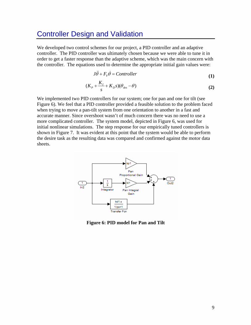
We implemented two PID controllers for our system; one for pan and one for tilt (see Figure 6). We feel that a PID controller provided a feasible solution to the problem faced when trying to move a pan-tilt system from one orientation to another in a fast and accurate manner. Since overshoot wasn’t of much concern there was no need to use a more complicated controller. The system model, depicted in Figure 6, was used for initial nonlinear simulations. The step response for our empirically tuned controllers is shown in Figure 7. It was evident at this point that the system would be able to perform the desire task as the resulting data was compared and confirmed against the motor data sheets.

Figure 6: PID model for Pan and Tilt

9

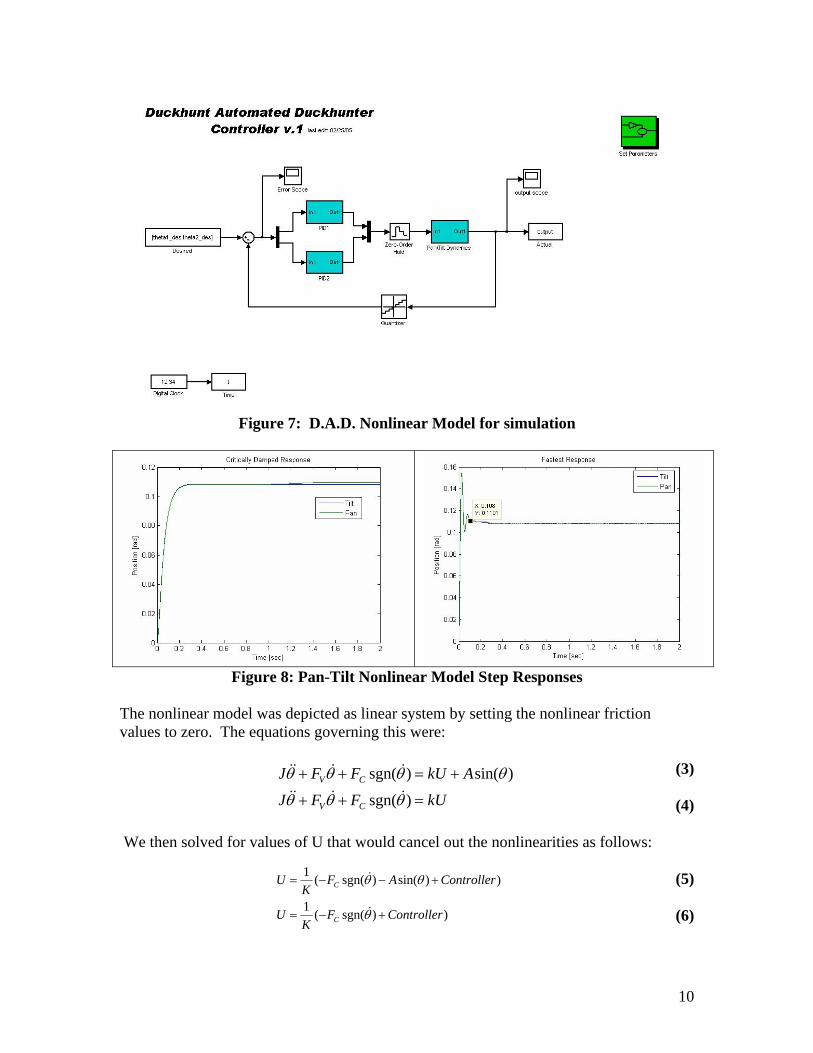
Figure 7: D.A.D. Nonlinear Model for simulation

Figure 8: Pan-Tilt Nonlinear Model Step Responses

The nonlinear model was depicted as linear system by setting the nonlinear friction values to zero. The equations governing this were:

(3) AkUFFJ +=+ )sgn( θθθθ

(4) kUFFJ =+ sgn(θθθ CV

CV

+

+

)

sin()

We then solved for values of U that would cancel out the nonlinearities as follows:

(5)

(6) ))

sgn((1K

U = θ

)sin()

ControllerF

FK

C

C

+−

−− )sgn((1 ControllerAU += θθ

10

At this point the controller and linear plant model had been fully defined. The next step was to validate that our controller could perform according to our system requirements. The validation was performed by sending varying signals to both the DAD system model as well as the actual system. The first response was to that of a sinusoidal input or tracking command. This is shown in Figure 9. The input command that was most useful to us was the step input since this is what is ultimately commanded the end DAD system. The results are shown in Figure 10. The steady state error was <0.7% for both the pan and tilt axis. The settling times were also right around the desired values of 200ms which led the group to a conclusion that our model was acceptable.

Figure 9: Model Validation – Tracking Command

Figure 10: Model Validation Zoom

11

Figure 11: System Step Response

A second controller was design to enhance these results. The calculated coefficients exist with some error, and having the controller built based off these coefficients are an added source of error in the system. In an attempt to minimize this error and adaptive scheme was introduced in the form of model reference adaptive control, or more specifically “simple adaptive control”. The purpose of an MRAC control is to force the plant to act like a model of the plant by dynamically manipulating the input of the plant to reach the desired results. The ideal result then would be to have a controller that could flawlessly control our model also flawlessly control our plant. The SAC controller called for altering the input of the plant by several values that directly correlated with the model and the difference between the model’s and the plant’s output:

dteeAeAA

dteyyAeyAA

dteuuAeuAA

iP

mmimP

mmimP

∫∫∫

+=

+=

+=

233

22

21

where and are adaptation gains, is the input to the model, is the output of the model, and is the difference between the model output and the plant’s output. From this a new control signal is built and sent to the plant as:

PA iA mu mye

muAAAu +++= 321

12

The adaptation gains were chosen to be small; since the PID controlled device was already within specification.

Figure 12: Simulink Implementation of SAC

With the SAC designed the PID controller was applied to the system and the following results were found.

Figure 13: Step Response for PID and PIS+SAC

13

Figure 14: Sinusoidal Tracking Response over Two Periods As was expected, the SAC implementation reduced the step response a bit, and also improved the steady state tracking error to within 4.5%, a 3% increase. Issues however arose during testing for disturbance rejection. The PID controller preformed flawlessly, treating instantaneous disturbances as steps. The SAC implementation had much lesser success however. Placing a small disturbance into the system resulted in a fairly lengthy response that did ultimately return to the wanted value; however a larger disturbance produced a very unstable response with little hope of returning to the required value in an acceptable amount of time. The reasoning for this implementation of MRAC’s lack of robustness is fairly easy to understand. The controller is based off of comparing the model’s output to the plant’s output, and error is incurred when they do not match. A disturbance applied to the plant is not applied to the model, and so the integrations of the error that are being used to drive the plant windup quadratically, resulting in a large response given a large enough error. A possible fix would be to implement an anti-windup feature that would reset the integral values to zero on a zero crossing, this however was not implemented. The final controller was then decided to be the purely PID controller described earlier in this section.

Figure 15: Implemented DAD system controller

14

Image Acquisition Our ability to succeed in this project was greatly dependent on our ability to acquire images from a webcam input. We needed to be able to acquire images at a quick enough rate in order to insure there would be enough time to process images. In order to do this a MATLAB m-script was written [see appendix F] that would direct the webcam to start logging data. A comparison between timestamps of the logged frames yields us the acquisition time. For runs collecting ten frames the average time was 0.0321 seconds between frames. The following is a sample capture from the webcam:

Figure 16: Webcam acquired images

As seen in Figure 16 the duck’s position remains relatively the same in all frames. This means that for the duration of the ten frames, 0.289 sec, a firing of the gun will register a hit during game play. This establishes a more clear timing requirement than the previous estimate of 0.200 sec, which was computed by measuring the duck’s flight length across the screen and trying to time with a stopwatch. The image that is produced by the web cam acts as a mapping of the environment where the duck target is located, leading to the function of image processing to resolve its exact location. With the aid of the MATLAB Image Processing Toolbox and utilizing their established functions we were able to change an acquired image shown in Figure 17 below to a processed image shown in Figure 18.

15

Figure 18: Processed Image

be done a template file is created to aid that might be mistaken for duck objects.

west color value possible in an image and age. So by subtracting the template

e the wanted target is the only object

Figure 17: Acquired Image

Before any processing of the acquired image is toin removing unwanted objects from the screen MATLAB associates the color black as the lowhite as the highest color value possible in an imimage in Figure 19 from the acquired imagremaining in Figure 20.

Figure 19: Template Image

The lines of code, bw = ~im2bw(A,duckupper) - ~[labeled,numObjects] = bwlabel(~bw,4);

both converts the image to binary and appwas tested to be .3 and .85 respectively foset of sampled processed images

Figure 20: Unwanted Objects

im2bw(A,ducklower); (7) (8)

lies a minimum and maximum threshold which r optimal image differentiation properties. A

is located below in Figure 21.

16

Figure 21: Set of Sample Processed Images

MATLAB produces two variables label and numObjects as outputs to the splicing function, where in label contains a vector of structures containing data concerning each object MATLAB recognized and numObjects contains the size of label. The MATLAB function regionprops gives attributes to the label vector based on a certain parameter, the default being basic.

data = regionprops(labeled,'basic')

he contents of data, the resulting vector, is then

where Area is the area of t age frame coordinate of the centroid of the object, and BoundingBox s the parameters of the smallest rectangle

rocess is then to search through the vector and establish which object is the target. To identify the appropriate object as the ta quires a small bit of logic regarding the location in the image and the size of the such the following conditions were used:

object is larger than 50 pixels

T

data = struct { Area

Centroid Boundingox}

he object identified, Centroid is the im i

that fits around the object. The remainder of the p

rget re object. As

TABLE 4: CONDITIONS FOR IMAGE DATA data(i).BoundingBox(2) <= 200

data(i).Area <= 400 data(i).Area >= 50

The object is above in the top 200 pixels The object is smaller than 400 pixels2

The 2

17

To amend the issue of multiple objects fulfilling these conditions a target vector is added to further analyze the objects and to define the 3 that are most appropriate. Such analysis of the image successfully returns the centroid, image coordinates, of the target as an output With the lo gets determ ngles to send to t ing at the ducks on the screen. This was done with the

nction,

)

ss. ls to aim the zapper was

latively simple to calculate. The image processing took on average 0.140 seconds.

within specifications.

for each of the test images, without fail.

cation of the duck tar ined all that is left to determine is the ahe controller for aim

fu

[xangle,yangle] = return_angles(xpos, ypos); (9

This function was created using the specifications developed earlier in the design proceMaking use of MATLAB’s trigonometric functions the angereDetermining the angle to aim the zapper was roughly 0.021 seconds on average. The totaltime for acquiring the angles to aim at the duck targets ended up being 0.161 seconds which was

18

Schedule

The D.A.D. project was broken down into several phases. Each phase was building block for the next and thus it had to be complete so that the project could continue. For this project, our plan of action was:

1. Initial System Development

Parameter Identification - Inertia matrices approximated using Solidworks modeling. Factors for Coulomb and viscous friction were established through experimentation. Automated MATLAB m-file and Simulink model generated to input specified torque to each axis independently and monitor velocity. Plots generated for torque vs. velocity to be output. Use of xPC Target for embedded control.

System Modeling - Simulink diagrams generated to simulate the dynamics of pan-tilt system. Using values from parameter identification and motor data sheets, simulation of desired control objective was performed.

2. Controller Design

Controller Modeling - Once it was determined that the system can perform our broad control objective using simulation. Plots were generated to show position output vs. time. This gave insight into how well the PID algorithm was performing. Controller Tuning - Using position vs. time data, the PID controller was tuned so that response was critically damped and still met control objective.

3. Sensors

Image Acquisition - USB webcam connected via host pc. Image acquisition study was performed in order to baseline timing capabilities of camera and MATLAB. Image Processing - MATLAB and Simulink models as well as image processing algorithms were developed in order to correlate duck on screen position to light gun positioning.

4. Integration

Integration - Webcam was used to provide desired angles to pan-tilt axis. Use of xPC Target for embedded control of pan-tilt system. Validation/ Testing - Comparison of simulated system response to actual system response and noise disturbance study.

19

5. System Performance Enhancements

Performance Enhancements – We were able to fine tune of control parameters to ensure accurate aiming at advanced game play speeds.

The schedule listed in Table 3 is a rough breakdown of individual tasks mentioned above. The overall project was scheduled to be completed well before deadline in order to allow for unforeseen development problems or project enhancements, which was needed. Overall, most of the smaller projects were completed as a whole team, which enhanced the design experience of each team member. Throughout the semester, we stayed very close to the proposed schedule from the start of this project. The challenges that we had with keeping with the original schedule was the image processing. This sub-project took much longer than we first thought it would. Therefore it was a good that we planned on challenges and gave ourselves time to overcome them.

TABLE 5: GANTT CHART OF SCHEDULE

20

Costs The cost analysis for D.A.D. project is based on material and labor costs. Labor costs were computed using the following formula:

Total Labor Cost = Estimated Fixed Costs + hourly wage * total project hours * 4 members

An estimated 100 hours was spent by each team member. Estimated fixed costs consist of rent and other extraneous laboratory expenses; estimated to be $3,000. A nominal starting hourly wage of $15 will be assumed, thus leading to total labor costs of $12,000. The material costs include assembled system, USB webcam, Nintendo Entertainment System with Zapper Light Gun and Duck Hunt video game cartridge. The total project expenditures are zero to date as all parts have either been provided by RPI or donated from team members. The total project cost breakdown is as follows:

TABLE 6: PROJECT COST BREAKDOWN

Index Individual Components Manufacturer Part Number Quantity Price Each 1 Pan Motor Pittman GM8712-11 1 $74.742 Tilt Motor Pittman GM8712-11 1 $74.743 Pan Motor Pulley SDP A 6A 6-20DF01806 1 $7.524 Tilt Motor Pulley SDP A 6A 6-20DF01806 1 $7.525 Pan Shaft Pulley SDP A 6A61-00NF01812 1 $18.616 Tilt Shaft Pulley SDP A 6A61-00NF01812 1 $18.617 Pan Timing Belt SDP A 6R 6-1350180 1 $3.028 Tilt Timing Belt SDP A 6R 6-1350180 1 $3.029 Shaft SDP A 7X 1-12060 2 $4.5610 Encoders US Digital S1-1024-B 2 $61.1011 Shaft Collars Ruland 1403377 2 $2.4812 Flex Coupling SDP S50MSC-A04H25H25 2 $15.7913 USB Webcam Logitech 861161-0000 1 $44.9914 NES with Gun & Duck Hunt Game Nintendo N/A 1 $25.9915 LabJack U12 LabJack N/A 1 $119.0016 Compact 5VDC/1A SPST Reed Relay RadioShack 275-232 1 $2.79

Material Total: $484.48 Estimated Labor Total: $12,000.00

Project Total: $12,484.48

21

Bibliography [1] Sozer, et al. “DMRAC of Permanent Magnet Brushless Motors.” Rensselaer ECSE Department, 1997

22

Team Member Contribution

Adam Blot __________________________

• Introduction

• Friction Identification

• Presentation

Morrigan McNamara __________________________

• Report Compilation

• Cost

• Presentation

• Final Video

Lloyd Mebane __________________________

• Image Acquisition

• Appendices

• Presentation

Aryn Shapiro __________________________

• System Modeling

• Controller Design and Validation

• Presentation

23

Appendix A – gains.m %DAD Project Parameters %ECSE Control Systems Design - Spring 2005 %Team 3 %Pan a1p = 33.8106; a2p = 32.6874; a3p = 1.0440; %Tilt a1t = 26.8061; a2t = 8.6386; a3t = 0.2759; a4t = .003; %Controller Ap = [0 1;0 -a2p]; Bp = [0 a1p]'; Cp = [1 0]; Lp = [-12.6874 414.7181]; %PID Gains kp1=700; ki1=.1; kd1=50; kp2=2300; ki2=.1; kd2=20; p=100; %Adaptive Gains Ayi = 1; Aui = 1; Aei = 1; Ayp = 1; Aup = 1; Aep = 1; thetax=0; thetay=0; vid=videoinput('winvideo',1); header='C:\Program Files\LabJack\drivers\ljackuw.h';

24

loadlibrary('ljackuw',header); tg=xpc; dad_final;

25

Appendix B – Fast Response Graph

26

Appendix C – Critical Response Graph

27

Appendix D – friction.m %% Friction Analysis % Ramp parameters m = .1; icr = -3; % run the target for 12 seconds start(tg); pause stop(tg); % get output data time = tg.timelog; vol = tg.outputlog(:,5); vel = tg.outputlog(:,4); % run target again adding up the output data for l=1:9 l start(tg); pause stop(tg); vel = (vel + tg.outputlog(:,4)); end % average the data to get a filtered/smooth curve vel = vel./10; % filter 60000 data to 600 for i = 1:(s/100) vo(i) = vel(100*i); vl(i) = vol(100*i); end % plot plot(vo,vl);grid xlabel('Velocity'); ylabel('Voltage'); title('Velocity vs Voltage');

28

Appendix E – find_duck2.m %function target = find_duck(A); %returns area bounding box and centroid of duck function [xpos,ypos,num,bw] = find_duck2(A);% returns centroid of duck % processimage into a black and white with the duck white (hopefully) %Edit below values for isolating ducks ducklower = .3;% lower bounds of duck threshold duckupper = 0.85;% upper bounds of duck threshold ground_pos = 200;% the pixel location of the ground duck_min = 25; % minimum size of duck duck_max = 200; % maximum size of duck % image processing bw = ~im2bw(A,duckupper) - ~im2bw(A,ducklower); [labeled,numObjects] = bwlabel(bw,4); % organises objects found in the image graindata = regionprops(labeled,'basic'); %pause num = 0; % scan objects for characteristic duck for i = 1:numObjects bill = 2; if bill > 0 if (graindata(i).BoundingBox(2) <= ground_pos) & (graindata(i).Area <= duck_max) & (graindata(i).Area >= duck_min) bill = 0; num = num + 1; end end %if duck is found if bill <= 0 % add duck x,y to target list target(num) = graindata(i); % pause end end if num >= 1 cent = target(1).Centroid; xpos = cent(1);

29

ypos = cent(2); else xpos = 500; ypos = 500; end %num = numObjects;

30

Appendix F – time test.m and output time graph Time_Test.m %This Program Tests time required to aquire image vid = videoinput('winvideo', 1);%sets up video start(vid); [data,time]=getdata(vid,10);%returns time, Fx1 data field, where F is frames elapsed_time1 = (time(2)-time(1))%computes time between frames elapsed_time2 = (time(3)-time(2)) elapsed_time3 = (time(4)-time(3)) elapsed_time4 = (time(5)-time(4)) elapsed_time5 = (time(6)-time(5)) elapsed_time6 = (time(7)-time(6)) elapsed_time7 = (time(8)-time(7)) elapsed_time8 = (time(9)-time(8)) elapsed_time9 = (time(10)-time(9)) imaqmontage(data); %displays all of the images captured with getdata Duck Flight Time Study elapsed_time1 = 0.0310 elapsed_time2 = 0.0330 elapsed_time3 = 0.0320 elapsed_time4 = 0.0310 elapsed_time5 = 0.0330 elapsed_time6 = 0.0340 elapsed_time7 = 0.0330 elapsed_time8 = 0.0300 elapsed_time9 = 0.0320 Total Time= 0.2890 sec Average Time= 0.0321 sec

31

Appendix G – Mounting Pictures

32

Appendix H – rlls.m %system model clear('theta2'); clear('theta'); clear('P'); start(tg); pause stop(tg); time = tg.timelog; yout = tg.outputlog; theta = [-1 .5 1 .5]; theta2(1,:) = theta; P(1).p = eye(4); err = 1; h = 1; k = 1; while (1) yt = yout(k,:); y = yt(1); phi = yt(2:5)'; P(k+1).p = (P(k).p) - 1/(1+phi'*(P(k).p)*phi)*(P(k).p)*phi*phi'*(P(k).p); theta(k+1,:) = theta(k,:)' + (P(k+1).p)*phi*(y-phi'*theta(k,:)'); if(k >= 1000) h=h+1; theta2(h,:) = theta(k+1,:); theta(1000,:) theta(2,:) = theta(k+1,:); err = norm(y-phi'*theta(k+1,:)') if err < .0000001 break end P(2).p = P(k+1).p; k = 1; end k = k +1; end disp('coeffs for pan'); theta(1000,:); clear('theta'); clear('P');

33

Appendix I – fire.m calllib('ljackuw','DigitalIO',-1,0,1,1,0,0,1,0) pause(.1) calllib('ljackuw','DigitalIO',-1,0,1,1,1,0,1,0)

34

Appendix J – return_angles.m function [xangle,yangle] = return_angles(xpos, ypos); %assuming 0 position is middle of screen ppi = 320/11.5; gdist = 25*ppi; sw = 11.5*ppi; sh = 9*ppi; ixmax = 320; iymax = 240; xtmax = asin((sw/2)/(gdist^2+(sw/2)^2)); ytmax = asin((sh/2)/(gdist^2+(sh/2)^2)); center = [ixmax/2 iymax/2]; %aim = duck-center; xp = asin((center(1)-xpos)/(gdist^2+(center(1)-xpos)^2)^(.5)); yp = asin((center(2)-ypos)/(gdist^2+(center(2)-ypos)^2)^(.5)); xangle = xp; yangle = yp;

35

Appendix K – temp_2.m %DAD project function [x,y,C] = temp_2(vid,tg); set(vid,'TriggerRepeat',Inf); B = imread('temp2.jpg'); %Move to default position setparam(tg,9,0); setparam(tg,10,0); stop(vid); start(vid); %[D T M ] = getdata(vid); %T curr_time = 0; fires = 0; while(1)%vid.FramesAcquired<=5) %[pic,time] = getdata(vid,1); pic = getdata(vid,1); %acquire image A = pic(:,:,:,1) - B; %process image and get x and y coordinates [x,y,num,bw]=find_duck2(A); if x <=400 & fires <= 3 %Pictures to see what temp file is blocking out and what find duck %is returning as a duck. % figure, imshow(A); % figure, imshow(bw); %take x and y pixel coordinates and return angles for gun to move [thetax,thetay] = return_angles(x,y); %aims light zapper at duck setparam(tg,9,thetax); setparam(tg,10,thetay); %delay for moving zapper pause(.02); %fires zapper at duck target fire; fires = fires + 1;

36

else if fires >= 3 pause(1.5); end fires = 0; curr_time = 0; end flushdata(vid,'triggers'); end stop(vid);

37

Appendix L – temp2.jpg

38

Appendix M – dad_final.mdl

39