financial time series user's guide -...
TRANSCRIPT
Computation
Visualization
Programming
For Use with MATLAB®
Financial Time SeriesToolbox
User’s GuideVersion 1
How to Contact The MathWorks:
508-647-7000 Phone
508-647-7001 Fax
The MathWorks, Inc. Mail3 Apple Hill DriveNatick, MA 01760-2098
http://www.mathworks.com Webftp.mathworks.com Anonymous FTP servercomp.soft-sys.matlab Newsgroup
[email protected] Technical [email protected] Product enhancement [email protected] Bug [email protected] Documentation error [email protected] Subscribing user [email protected] Order status, license renewals, [email protected] Sales, pricing, and general information
Financial Time Series Toolbox User’s Guide COPYRIGHT 1999 by The MathWorks, Inc. The software described in this document is furnished under a license agreement. The software may be used or copied only under the terms of the license agreement. No part of this manual may be photocopied or repro-duced in any form without prior written consent from The MathWorks, Inc.
FEDERAL ACQUISITION: This provision applies to all acquisitions of the Program and Documentation by or for the federal government of the United States. By accepting delivery of the Program, the government hereby agrees that this software qualifies as "commercial" computer software within the meaning of FAR Part 12.212, DFARS Part 227.7202-1, DFARS Part 227.7202-3, DFARS Part 252.227-7013, and DFARS Part 252.227-7014. The terms and conditions of The MathWorks, Inc. Software License Agreement shall pertain to the government’s use and disclosure of the Program and Documentation, and shall supersede any conflicting contractual terms or conditions. If this license fails to meet the government’s minimum needs or is inconsistent in any respect with federal procurement law, the government agrees to return the Program and Documentation, unused, to MathWorks.
MATLAB, Simulink, Stateflow, Handle Graphics, and Real-Time Workshop are registered trademarks, and Target Language Compiler is a trademark of The MathWorks, Inc.
Other product or brand names are trademarks or registered trademarks of their respective holders.
Printing History: July 1999 First printing New for Version 1.0

Contents
Preface
About this Book . . . . . . . . . . . . . . . . . . . . . . . . . . . . . . . . . . . . . . . viOrganization of the Document . . . . . . . . . . . . . . . . . . . . . . . . . . . viTypographical Conventions . . . . . . . . . . . . . . . . . . . . . . . . . . . . . vi
Related Products . . . . . . . . . . . . . . . . . . . . . . . . . . . . . . . . . . . . . viii
Required Software . . . . . . . . . . . . . . . . . . . . . . . . . . . . . . . . . . . . . . x
Online Tutorials . . . . . . . . . . . . . . . . . . . . . . . . . . . . . . . . . . . . . . . xi
1Tutorial
Introduction . . . . . . . . . . . . . . . . . . . . . . . . . . . . . . . . . . . . . . . . . 1-2
Creating Financial Time Series Objects . . . . . . . . . . . . . . . . . 1-3Using the Constructor . . . . . . . . . . . . . . . . . . . . . . . . . . . . . . . . . 1-3Transforming a Text File . . . . . . . . . . . . . . . . . . . . . . . . . . . . . 1-10
Working with Financial Time Series Objects . . . . . . . . . . . 1-13Financial Time Series Object Structure . . . . . . . . . . . . . . . . . . 1-13Data Extraction . . . . . . . . . . . . . . . . . . . . . . . . . . . . . . . . . . . . . 1-13Object to Matrix Conversion . . . . . . . . . . . . . . . . . . . . . . . . . . . 1-15Indexing a Financial Time Series Object . . . . . . . . . . . . . . . . . 1-17Operations . . . . . . . . . . . . . . . . . . . . . . . . . . . . . . . . . . . . . . . . . 1-22Data Transformation and Frequency Conversion . . . . . . . . . . 1-26
Technical Analysis . . . . . . . . . . . . . . . . . . . . . . . . . . . . . . . . . . . 1-31Examples . . . . . . . . . . . . . . . . . . . . . . . . . . . . . . . . . . . . . . . . . . 1-33
i
ii Contents
Demonstration Program . . . . . . . . . . . . . . . . . . . . . . . . . . . . . . 1-39Load the Data . . . . . . . . . . . . . . . . . . . . . . . . . . . . . . . . . . . . . . . 1-39Create Financial Time Series Objects . . . . . . . . . . . . . . . . . . . . 1-40Create Closing Prices Adjustment Series . . . . . . . . . . . . . . . . . 1-41Adjust Closing Prices and Make Them Spot Prices . . . . . . . . . 1-41Create Return Series . . . . . . . . . . . . . . . . . . . . . . . . . . . . . . . . . 1-42Regress Return Series Against Metric Data . . . . . . . . . . . . . . 1-42Plot the Results . . . . . . . . . . . . . . . . . . . . . . . . . . . . . . . . . . . . . 1-43Calculate the Dividend Rate . . . . . . . . . . . . . . . . . . . . . . . . . . . 1-44
2Function Reference
Functions by Category . . . . . . . . . . . . . . . . . . . . . . . . . . . . . . . . 2-2
Alphabetical List of Functions . . . . . . . . . . . . . . . . . . . . . . . . . 2-9adline . . . . . . . . . . . . . . . . . . . . . . . . . . . . . . . . . . . . . . . . . . . . . 2-12adosc . . . . . . . . . . . . . . . . . . . . . . . . . . . . . . . . . . . . . . . . . . . . . . 2-15ascii2fts . . . . . . . . . . . . . . . . . . . . . . . . . . . . . . . . . . . . . . . . . . . . 2-17bollinger . . . . . . . . . . . . . . . . . . . . . . . . . . . . . . . . . . . . . . . . . . . 2-18boxcox . . . . . . . . . . . . . . . . . . . . . . . . . . . . . . . . . . . . . . . . . . . . . 2-20busdays . . . . . . . . . . . . . . . . . . . . . . . . . . . . . . . . . . . . . . . . . . . . 2-22candle . . . . . . . . . . . . . . . . . . . . . . . . . . . . . . . . . . . . . . . . . . . . . 2-23chaikosc . . . . . . . . . . . . . . . . . . . . . . . . . . . . . . . . . . . . . . . . . . . 2-25chaikvolat . . . . . . . . . . . . . . . . . . . . . . . . . . . . . . . . . . . . . . . . . . 2-28chartfts . . . . . . . . . . . . . . . . . . . . . . . . . . . . . . . . . . . . . . . . . . . . 2-31chfield . . . . . . . . . . . . . . . . . . . . . . . . . . . . . . . . . . . . . . . . . . . . . 2-33convertto . . . . . . . . . . . . . . . . . . . . . . . . . . . . . . . . . . . . . . . . . . . 2-34demts2fts . . . . . . . . . . . . . . . . . . . . . . . . . . . . . . . . . . . . . . . . . . 2-35diff . . . . . . . . . . . . . . . . . . . . . . . . . . . . . . . . . . . . . . . . . . . . . . . . 2-36display . . . . . . . . . . . . . . . . . . . . . . . . . . . . . . . . . . . . . . . . . . . . . 2-37end . . . . . . . . . . . . . . . . . . . . . . . . . . . . . . . . . . . . . . . . . . . . . . . . 2-38exp . . . . . . . . . . . . . . . . . . . . . . . . . . . . . . . . . . . . . . . . . . . . . . . . 2-40extfield . . . . . . . . . . . . . . . . . . . . . . . . . . . . . . . . . . . . . . . . . . . . 2-41fieldnames . . . . . . . . . . . . . . . . . . . . . . . . . . . . . . . . . . . . . . . . . 2-42fillts . . . . . . . . . . . . . . . . . . . . . . . . . . . . . . . . . . . . . . . . . . . . . . . 2-43filter . . . . . . . . . . . . . . . . . . . . . . . . . . . . . . . . . . . . . . . . . . . . . . 2-44

fints . . . . . . . . . . . . . . . . . . . . . . . . . . . . . . . . . . . . . . . . . . . . . . . 2-45fpctkd . . . . . . . . . . . . . . . . . . . . . . . . . . . . . . . . . . . . . . . . . . . . . 2-47freqnum . . . . . . . . . . . . . . . . . . . . . . . . . . . . . . . . . . . . . . . . . . . 2-50freqstr . . . . . . . . . . . . . . . . . . . . . . . . . . . . . . . . . . . . . . . . . . . . . 2-51fts2ascii . . . . . . . . . . . . . . . . . . . . . . . . . . . . . . . . . . . . . . . . . . . . 2-52fts2mtx . . . . . . . . . . . . . . . . . . . . . . . . . . . . . . . . . . . . . . . . . . . . 2-53ftsbound . . . . . . . . . . . . . . . . . . . . . . . . . . . . . . . . . . . . . . . . . . . 2-54getfield . . . . . . . . . . . . . . . . . . . . . . . . . . . . . . . . . . . . . . . . . . . . 2-55getnameidx . . . . . . . . . . . . . . . . . . . . . . . . . . . . . . . . . . . . . . . . . 2-56hhigh . . . . . . . . . . . . . . . . . . . . . . . . . . . . . . . . . . . . . . . . . . . . . . 2-57highlow . . . . . . . . . . . . . . . . . . . . . . . . . . . . . . . . . . . . . . . . . . . . 2-59hist . . . . . . . . . . . . . . . . . . . . . . . . . . . . . . . . . . . . . . . . . . . . . . . 2-61horzcat . . . . . . . . . . . . . . . . . . . . . . . . . . . . . . . . . . . . . . . . . . . . 2-63iscompatible . . . . . . . . . . . . . . . . . . . . . . . . . . . . . . . . . . . . . . . . 2-65isequal . . . . . . . . . . . . . . . . . . . . . . . . . . . . . . . . . . . . . . . . . . . . . 2-66isfield . . . . . . . . . . . . . . . . . . . . . . . . . . . . . . . . . . . . . . . . . . . . . 2-67lagts . . . . . . . . . . . . . . . . . . . . . . . . . . . . . . . . . . . . . . . . . . . . . . 2-68leadts . . . . . . . . . . . . . . . . . . . . . . . . . . . . . . . . . . . . . . . . . . . . . . 2-69length . . . . . . . . . . . . . . . . . . . . . . . . . . . . . . . . . . . . . . . . . . . . . 2-70llow . . . . . . . . . . . . . . . . . . . . . . . . . . . . . . . . . . . . . . . . . . . . . . . 2-71log . . . . . . . . . . . . . . . . . . . . . . . . . . . . . . . . . . . . . . . . . . . . . . . . 2-73log10 . . . . . . . . . . . . . . . . . . . . . . . . . . . . . . . . . . . . . . . . . . . . . . 2-74macd . . . . . . . . . . . . . . . . . . . . . . . . . . . . . . . . . . . . . . . . . . . . . . 2-75max . . . . . . . . . . . . . . . . . . . . . . . . . . . . . . . . . . . . . . . . . . . . . . . 2-77mean . . . . . . . . . . . . . . . . . . . . . . . . . . . . . . . . . . . . . . . . . . . . . . 2-78medprice . . . . . . . . . . . . . . . . . . . . . . . . . . . . . . . . . . . . . . . . . . . 2-79min . . . . . . . . . . . . . . . . . . . . . . . . . . . . . . . . . . . . . . . . . . . . . . . 2-81minus . . . . . . . . . . . . . . . . . . . . . . . . . . . . . . . . . . . . . . . . . . . . . 2-82mrdivide . . . . . . . . . . . . . . . . . . . . . . . . . . . . . . . . . . . . . . . . . . . 2-83mtimes . . . . . . . . . . . . . . . . . . . . . . . . . . . . . . . . . . . . . . . . . . . . 2-84negvolidx . . . . . . . . . . . . . . . . . . . . . . . . . . . . . . . . . . . . . . . . . . . 2-85onbalvol . . . . . . . . . . . . . . . . . . . . . . . . . . . . . . . . . . . . . . . . . . . . 2-87peravg . . . . . . . . . . . . . . . . . . . . . . . . . . . . . . . . . . . . . . . . . . . . . 2-89plot . . . . . . . . . . . . . . . . . . . . . . . . . . . . . . . . . . . . . . . . . . . . . . . 2-90plus . . . . . . . . . . . . . . . . . . . . . . . . . . . . . . . . . . . . . . . . . . . . . . . 2-92posvolidx . . . . . . . . . . . . . . . . . . . . . . . . . . . . . . . . . . . . . . . . . . . 2-93power . . . . . . . . . . . . . . . . . . . . . . . . . . . . . . . . . . . . . . . . . . . . . . 2-95prcroc . . . . . . . . . . . . . . . . . . . . . . . . . . . . . . . . . . . . . . . . . . . . . 2-96pvtrend . . . . . . . . . . . . . . . . . . . . . . . . . . . . . . . . . . . . . . . . . . . . 2-98rdivide . . . . . . . . . . . . . . . . . . . . . . . . . . . . . . . . . . . . . . . . . . . . 2-100
iii

iv Contents
resamplets . . . . . . . . . . . . . . . . . . . . . . . . . . . . . . . . . . . . . . . . 2-101rmfield . . . . . . . . . . . . . . . . . . . . . . . . . . . . . . . . . . . . . . . . . . . 2-102rsindex . . . . . . . . . . . . . . . . . . . . . . . . . . . . . . . . . . . . . . . . . . . 2-103 setfield . . . . . . . . . . . . . . . . . . . . . . . . . . . . . . . . . . . . . . . . . . . 2-105size . . . . . . . . . . . . . . . . . . . . . . . . . . . . . . . . . . . . . . . . . . . . . . 2-106smoothts . . . . . . . . . . . . . . . . . . . . . . . . . . . . . . . . . . . . . . . . . . 2-107sortfts . . . . . . . . . . . . . . . . . . . . . . . . . . . . . . . . . . . . . . . . . . . . 2-109spctkd . . . . . . . . . . . . . . . . . . . . . . . . . . . . . . . . . . . . . . . . . . . . 2-110std . . . . . . . . . . . . . . . . . . . . . . . . . . . . . . . . . . . . . . . . . . . . . . . 2-113stochosc . . . . . . . . . . . . . . . . . . . . . . . . . . . . . . . . . . . . . . . . . . . 2-114subsasgn . . . . . . . . . . . . . . . . . . . . . . . . . . . . . . . . . . . . . . . . . . 2-117subsref . . . . . . . . . . . . . . . . . . . . . . . . . . . . . . . . . . . . . . . . . . . 2-118times . . . . . . . . . . . . . . . . . . . . . . . . . . . . . . . . . . . . . . . . . . . . . 2-121toannual . . . . . . . . . . . . . . . . . . . . . . . . . . . . . . . . . . . . . . . . . . 2-122todaily . . . . . . . . . . . . . . . . . . . . . . . . . . . . . . . . . . . . . . . . . . . . 2-123todecimal . . . . . . . . . . . . . . . . . . . . . . . . . . . . . . . . . . . . . . . . . 2-124tomonthly . . . . . . . . . . . . . . . . . . . . . . . . . . . . . . . . . . . . . . . . . 2-125toquarterly . . . . . . . . . . . . . . . . . . . . . . . . . . . . . . . . . . . . . . . . 2-126toquoted . . . . . . . . . . . . . . . . . . . . . . . . . . . . . . . . . . . . . . . . . . 2-127tosemi . . . . . . . . . . . . . . . . . . . . . . . . . . . . . . . . . . . . . . . . . . . . 2-128toweekly . . . . . . . . . . . . . . . . . . . . . . . . . . . . . . . . . . . . . . . . . . 2-129tsaccel . . . . . . . . . . . . . . . . . . . . . . . . . . . . . . . . . . . . . . . . . . . . 2-130tsmom . . . . . . . . . . . . . . . . . . . . . . . . . . . . . . . . . . . . . . . . . . . . 2-132tsmovavg . . . . . . . . . . . . . . . . . . . . . . . . . . . . . . . . . . . . . . . . . . 2-134typprice . . . . . . . . . . . . . . . . . . . . . . . . . . . . . . . . . . . . . . . . . . . 2-137uminus . . . . . . . . . . . . . . . . . . . . . . . . . . . . . . . . . . . . . . . . . . . 2-139uplus . . . . . . . . . . . . . . . . . . . . . . . . . . . . . . . . . . . . . . . . . . . . . 2-140vertcat . . . . . . . . . . . . . . . . . . . . . . . . . . . . . . . . . . . . . . . . . . . . 2-141volroc . . . . . . . . . . . . . . . . . . . . . . . . . . . . . . . . . . . . . . . . . . . . . 2-142wclose . . . . . . . . . . . . . . . . . . . . . . . . . . . . . . . . . . . . . . . . . . . . 2-144willad . . . . . . . . . . . . . . . . . . . . . . . . . . . . . . . . . . . . . . . . . . . . 2-146willpctr . . . . . . . . . . . . . . . . . . . . . . . . . . . . . . . . . . . . . . . . . . . 2-148
Organization of the Document . . . . . . . . . . . . . . viTypographical Conventions . . . . . . . . . . . . . . . vi
Related Products . . . . . . . . . . . . . . . . . . viii
Required Software . . . . . . . . . . . . . . . . . . x
Online Tutorials . . . . . . . . . . . . . . . . . . . xi
Preface
About this Book . . . . . . . . . . . . . . . . . . . vi

Preface
vi
About this BookThis book describes the Financial Time Series Toolbox for MATLAB, a collection of tools for the analysis of time series data in the financial markets. Financial engineers working with time series data, such as equity prices or daily interest fluctuations, can use this toolbox for more intuitive data management than with regular vectors or matrices.
Organization of the Document
Typographical ConventionsWe use some or all of these conventions in our manuals.
Chapter Description
Chapter 1 “Tutorial”
Describes the creation, manipulation, and use of financial time series objects.
Chapter 2 “Function Reference”
Describes the functions used to create and manipulate financial time series objects. Also describes functions that use financial time series data in various financial indicators.
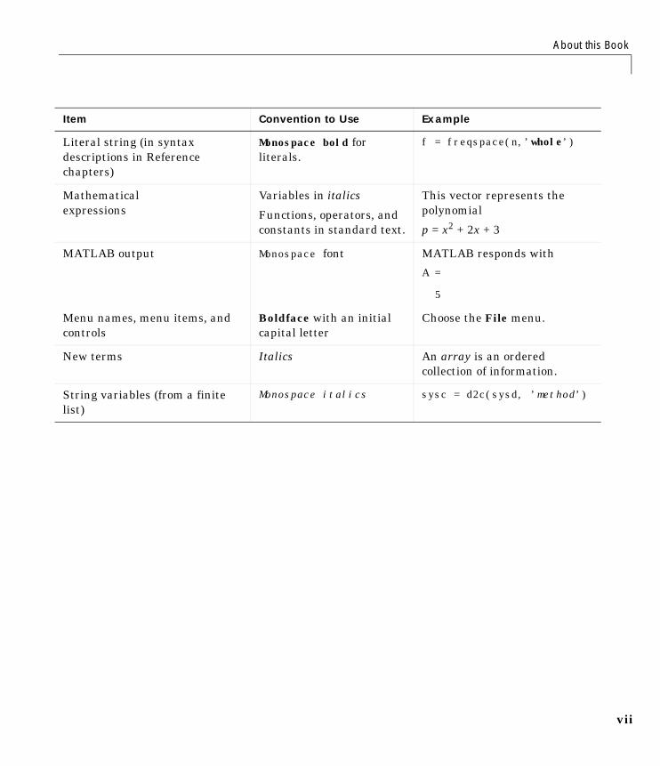
Item Convention to Use Example
Example code Monospace font To assign the value 5 to A, enter
A = 5
Function names/syntax Monospace font The cos function finds the cosine of each array element.
Syntax line example is
MLGetVar ML_var_name
Keys Boldface with an initial capital letter
Press the Return key.
About this Book
Literal string (in syntax descriptions in Reference chapters)
Monospace bold for literals.
f = freqspace(n,’whole’)
Mathematicalexpressions
Variables in italics
Functions, operators, and constants in standard text.
This vector represents the polynomial
p = x2 + 2x + 3
MATLAB output Monospace font MATLAB responds with
A =
5
Menu names, menu items, and controls
Boldface with an initial capital letter
Choose the File menu.
New terms Italics An array is an ordered collection of information.
String variables (from a finite list)
Monospace italics sysc = d2c(sysd, ’method’)
Item Convention to Use Example
vii
Preface
vii
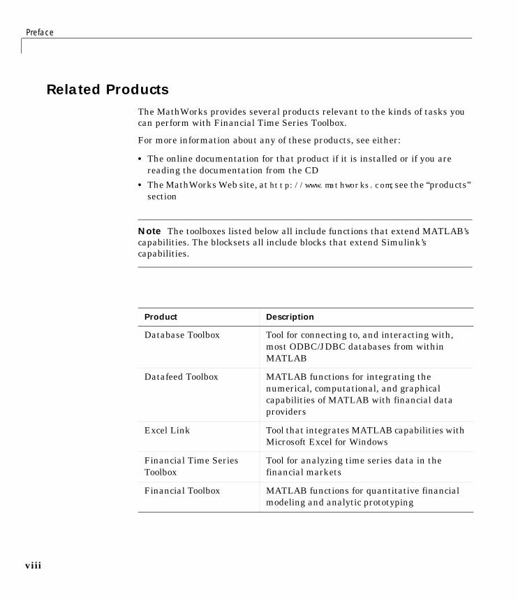
Related ProductsThe MathWorks provides several products relevant to the kinds of tasks you can perform with Financial Time Series Toolbox.
For more information about any of these products, see either:
• The online documentation for that product if it is installed or if you are reading the documentation from the CD
• The MathWorks Web site, at http://www.mathworks.com; see the “products” section
Note The toolboxes listed below all include functions that extend MATLAB’s capabilities. The blocksets all include blocks that extend Simulink’s capabilities.
Product Description
Database Toolbox Tool for connecting to, and interacting with, most ODBC/JDBC databases from within MATLAB
Datafeed Toolbox MATLAB functions for integrating the numerical, computational, and graphical capabilities of MATLAB with financial data providers
Excel Link Tool that integrates MATLAB capabilities with Microsoft Excel for Windows
Financial Time Series Toolbox
Tool for analyzing time series data in the financial markets
Financial Toolbox MATLAB functions for quantitative financial modeling and analytic prototyping
i
Related Products
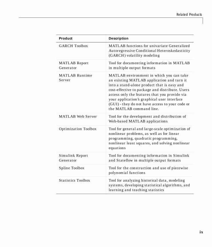
GARCH Toolbox MATLAB functions for univariate Generalized Autoregressive Conditional Heteroskedasticity (GARCH) volatility modeling
MATLAB Report Generator
Tool for documenting information in MATLAB in multiple output formats
MATLAB Runtime Server
MATLAB environment in which you can take an existing MATLAB application and turn it into a stand-alone product that is easy and cost-effective to package and distribute. Users access only the features that you provide via your application’s graphical user interface (GUI) - they do not have access to your code or the MATLAB command line.
MATLAB Web Server Tool for the development and distribution of Web-based MATLAB applications
Optimization Toolbox Tool for general and large-scale optimization of nonlinear problems, as well as for linear programming, quadratic programming, nonlinear least squares, and solving nonlinear equations
Simulink Report Generator
Tool for documenting information in Simulink and Stateflow in multiple output formats
Spline Toolbox Tool for the construction and use of piecewise polynomial functions
Statistics Toolbox Tool for analyzing historical data, modeling systems, developing statistical algorithms, and learning and teaching statistics
Product Description
ix

Preface
x
Required SoftwareThe Financial Time Series Toolbox requires:
• MATLAB Release 11 or later
• Financial Toolbox Version 2.0 or later
No other products are required.

Online Tutorials
Online TutorialsYou can find a set of three M-file tutorial scripts in the directory /toolbox/ftseries/ftstutorials on your MATLAB path. The scripts are named intro_fints, using_fints, and tech_analysis. Working through these tutorials can further introduce you to the Financial Time Series Toolbox.
xi

Preface
xii

Creating Financial Time Series Objects . . . . . . . 1-3Using the Constructor . . . . . . . . . . . . . . . . 1-3Transforming a Text File . . . . . . . . . . . . . . . 1-10
Working with Financial Time Series Objects . . . . . 1-13Financial Time Series Object Structure . . . . . . . . . 1-13Data Extraction . . . . . . . . . . . . . . . . . . . 1-13Object to Matrix Conversion . . . . . . . . . . . . . . 1-15Indexing a Financial Time Series Object . . . . . . . . . 1-17Operations . . . . . . . . . . . . . . . . . . . . . 1-22Data Transformation and Frequency Conversion . . . . . . 1-26
Technical Analysis . . . . . . . . . . . . . . . . . 1-31Examples . . . . . . . . . . . . . . . . . . . . . . 1-33
Demonstration Program . . . . . . . . . . . . . . 1-39Load the Data . . . . . . . . . . . . . . . . . . . . 1-39Create Financial Time Series Objects . . . . . . . . . . 1-40Create Closing Prices Adjustment Series . . . . . . . . . 1-41Adjust Closing Prices and Make Them Spot Prices . . . . . 1-41Create Return Series . . . . . . . . . . . . . . . . . 1-42Regress Return Series Against Metric Data . . . . . . . . 1-42Plot the Results . . . . . . . . . . . . . . . . . . . 1-43Calculate the Dividend Rate . . . . . . . . . . . . . . 1-44
1
Tutorial
Introduction . . . . . . . . . . . . . . . . . . . . 1-2
1 Tutorial
1-2
IntroductionThe Financial Time Series Toolbox for MATLAB is a collection of tools for the analysis of time series data in the financial markets. The toolbox contains a financial time series object constructor and several methods that operate on and analyze the object. Financial engineers working with time series data, such as equity prices or daily interest fluctuations, can use this toolbox for more intuitive data management than by using regular vectors or matrices.
This chapter discusses how to create and analyze financial time series data, including these topics:
• “Creating Financial Time Series Objects” on page 1-3
• “Working with Financial Time Series Objects” on page 1-13
• “Technical Analysis” on page 1-31
A “Demonstration Program” showing the use of financial time series data in a practical application is also included.

Creating Financial Time Series Objects
Creating Financial Time Series ObjectsThe Financial Time Series Toolbox provides two ways to create a financial time series object:
1 At the command line using the object constructor fints
2 From a text data file through the function ascii2fts
The structure of the object minimally consists of a description field, a frequency indicator field, the date vector, and a data series vector. The names for the fields are fixed for the first three fields: desc, freq, and dates. The user can specify the name for the data series vector. If a name is not specified, it defaults to series1. If the object has additional data series, the defaults are series2, series3, etc.
Using the ConstructorThe object constructor function fints has five different syntaxes. These forms exist to simplify object construction. The syntaxes are:
1 fts = fints(dates_and_data)
In this simplest form of syntax, the input must be at least a two-column matrix. The first column contains the dates in serial date format; the second column is the data series. The input matrix can have more than two columns, each additional column representing a different data series or set of observations.
If the input is a two-column matrix, the output object contains four fields: desc, freq, dates, and series1. The description field, desc, defaults to blanks ’’, and the frequency indicator field, freq, defaults to 0. The dates field, dates, contains the serial dates from the first column of the input matrix, while the data series field, series1, has the data from the second column of the input matrix.
The first example makes two financial time series objects. The first one has only one data series, while the other has more than one. A random vector provides the values for the data series. The range of dates is arbitrarily chosen using the today function.
date_series = (today:today+100)’;data_series = exp(randn(1, 101))’;
1-3
1 Tutorial
1-4
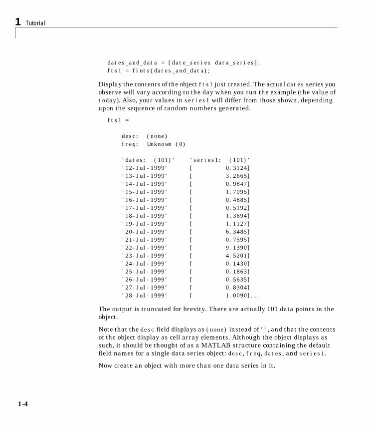
dates_and_data = [date_series data_series];fts1 = fints(dates_and_data);
Display the contents of the object fts1 just created. The actual dates series you observe will vary according to the day when you run the example (the value of today). Also, your values in series1 will differ from those shown, depending upon the sequence of random numbers generated.
fts1 =
desc: (none)freq: Unknown (0)
’dates: (101)’ ’series1: (101)’’12-Jul-1999’ [ 0.3124]’13-Jul-1999’ [ 3.2665]’14-Jul-1999’ [ 0.9847]’15-Jul-1999’ [ 1.7095]’16-Jul-1999’ [ 0.4885]’17-Jul-1999’ [ 0.5192]’18-Jul-1999’ [ 1.3694]’19-Jul-1999’ [ 1.1127]’20-Jul-1999’ [ 6.3485]’21-Jul-1999’ [ 0.7595]’22-Jul-1999’ [ 9.1390]’23-Jul-1999’ [ 4.5201]’24-Jul-1999’ [ 0.1430]’25-Jul-1999’ [ 0.1863]’26-Jul-1999’ [ 0.5635]’27-Jul-1999’ [ 0.8304]’28-Jul-1999’ [ 1.0090]...
The output is truncated for brevity. There are actually 101 data points in the object.
Note that the desc field displays as (none) instead of ’’, and that the contents of the object display as cell array elements. Although the object displays as such, it should be thought of as a MATLAB structure containing the default field names for a single data series object: desc, freq, dates, and series1.
Now create an object with more than one data series in it.
Creating Financial Time Series Objects
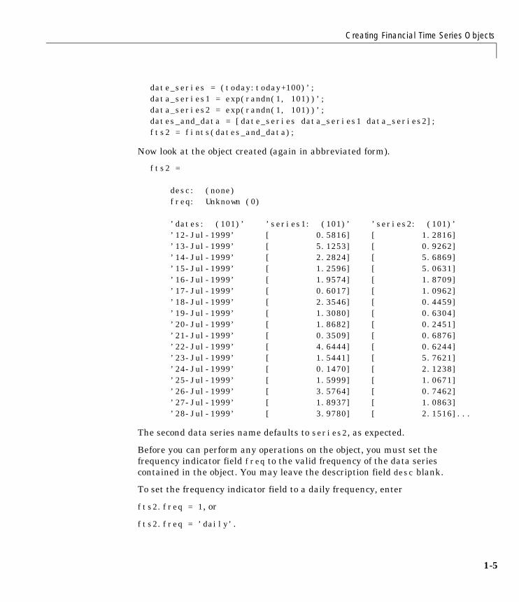
date_series = (today:today+100)’;data_series1 = exp(randn(1, 101))’;data_series2 = exp(randn(1, 101))’;dates_and_data = [date_series data_series1 data_series2];fts2 = fints(dates_and_data);
Now look at the object created (again in abbreviated form).
fts2 =
desc: (none)freq: Unknown (0)
’dates: (101)’ ’series1: (101)’ ’series2: (101)’’12-Jul-1999’ [ 0.5816] [ 1.2816]’13-Jul-1999’ [ 5.1253] [ 0.9262]’14-Jul-1999’ [ 2.2824] [ 5.6869]’15-Jul-1999’ [ 1.2596] [ 5.0631]’16-Jul-1999’ [ 1.9574] [ 1.8709]’17-Jul-1999’ [ 0.6017] [ 1.0962]’18-Jul-1999’ [ 2.3546] [ 0.4459]’19-Jul-1999’ [ 1.3080] [ 0.6304]’20-Jul-1999’ [ 1.8682] [ 0.2451]’21-Jul-1999’ [ 0.3509] [ 0.6876]’22-Jul-1999’ [ 4.6444] [ 0.6244]’23-Jul-1999’ [ 1.5441] [ 5.7621]’24-Jul-1999’ [ 0.1470] [ 2.1238]’25-Jul-1999’ [ 1.5999] [ 1.0671]’26-Jul-1999’ [ 3.5764] [ 0.7462]’27-Jul-1999’ [ 1.8937] [ 1.0863]’28-Jul-1999’ [ 3.9780] [ 2.1516]...
The second data series name defaults to series2, as expected.
Before you can perform any operations on the object, you must set the frequency indicator field freq to the valid frequency of the data series contained in the object. You may leave the description field desc blank.
To set the frequency indicator field to a daily frequency, enter
fts2.freq = 1, or
fts2.freq = ’daily’.
1-5

1 Tutorial
1-6
See the fints function description in the “Function Reference” for a list of frequency indicators.
2 fts = fints(dates, data)
In the second syntax the dates and data series are entered as separate vectors to fints, the financial time series object constructor function. The dates vector must be a column vector, while the data series data can be a column vector (if there is only one data series) or a column-oriented matrix (for multiple data series). A column-oriented matrix, in this context, indicates that each column is a set of observations. Different columns are different sets of data series.
Here is an example.
dates = (today:today+100)’;data_series1 = exp(randn(1, 101))’;data_series2 = exp(randn(1, 101))’;data = [data_series1 data_series2];fts = fints(dates, data)
fts =
desc: (none)freq: Unknown (0)
’dates: (101)’ ’series1: (101)’ ’series2: (101)’’12-Jul-1999’ [ 0.5816] [ 1.2816]’13-Jul-1999’ [ 5.1253] [ 0.9262]’14-Jul-1999’ [ 2.2824] [ 5.6869]’15-Jul-1999’ [ 1.2596] [ 5.0631]’16-Jul-1999’ [ 1.9574] [ 1.8709]’17-Jul-1999’ [ 0.6017] [ 1.0962]’18-Jul-1999’ [ 2.3546] [ 0.4459]’19-Jul-1999’ [ 1.3080] [ 0.6304]’20-Jul-1999’ [ 1.8682] [ 0.2451]’21-Jul-1999’ [ 0.3509] [ 0.6876]’22-Jul-1999’ [ 4.6444] [ 0.6244]’23-Jul-1999’ [ 1.5441] [ 5.7621]’24-Jul-1999’ [ 0.1470] [ 2.1238]’25-Jul-1999’ [ 1.5999] [ 1.0671]’26-Jul-1999’ [ 3.5764] [ 0.7462]’27-Jul-1999’ [ 1.8937] [ 1.0863]

Creating Financial Time Series Objects
’28-Jul-1999’ [ 3.9780] [ 2.1516]...
The result is exactly the same as the first syntax. The only difference between the first and second syntax is the way the inputs are entered into the constructor function.
3 fts = fints(dates, data, datanames)
The third syntax lets you specify the names for the data series with the argument datanames. datanames may be a MATLAB string for a single data series. For multiple data series names, it must be a cell array of string(s).
Look at two examples, one with a single data series and a second with two. The first example sets the data series name to the specified name First.
dates = (today:today+100)’;data = exp(randn(1, 101))’;fts1 = fints(dates, data, ’First’)
fts1 =
desc: (none)freq: Unknown (0)
’dates: (101)’ ’First: (101)’’12-Jul-1999’ [ 0.4615]’13-Jul-1999’ [ 1.1640]’14-Jul-1999’ [ 0.7140]’15-Jul-1999’ [ 2.6400]’16-Jul-1999’ [ 0.8983]’17-Jul-1999’ [ 2.7552]’18-Jul-1999’ [ 0.6217]’19-Jul-1999’ [ 1.0714]’20-Jul-1999’ [ 1.4897]’21-Jul-1999’ [ 3.0536]’22-Jul-1999’ [ 1.8598]’23-Jul-1999’ [ 0.7500]’24-Jul-1999’ [ 0.2537]’25-Jul-1999’ [ 0.5037]’26-Jul-1999’ [ 1.3933]’27-Jul-1999’ [ 0.3687]...
1-7
1 Tutorial
1-8
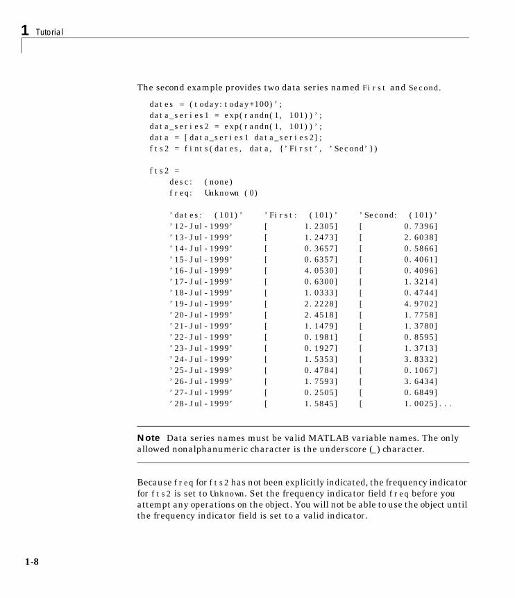
The second example provides two data series named First and Second.
dates = (today:today+100)’;data_series1 = exp(randn(1, 101))’;data_series2 = exp(randn(1, 101))’;data = [data_series1 data_series2];fts2 = fints(dates, data, {’First’, ’Second’})
fts2 = desc: (none)freq: Unknown (0)
’dates: (101)’ ’First: (101)’ ’Second: (101)’’12-Jul-1999’ [ 1.2305] [ 0.7396]’13-Jul-1999’ [ 1.2473] [ 2.6038]’14-Jul-1999’ [ 0.3657] [ 0.5866]’15-Jul-1999’ [ 0.6357] [ 0.4061]’16-Jul-1999’ [ 4.0530] [ 0.4096]’17-Jul-1999’ [ 0.6300] [ 1.3214]’18-Jul-1999’ [ 1.0333] [ 0.4744]’19-Jul-1999’ [ 2.2228] [ 4.9702]’20-Jul-1999’ [ 2.4518] [ 1.7758]’21-Jul-1999’ [ 1.1479] [ 1.3780]’22-Jul-1999’ [ 0.1981] [ 0.8595]’23-Jul-1999’ [ 0.1927] [ 1.3713]’24-Jul-1999’ [ 1.5353] [ 3.8332]’25-Jul-1999’ [ 0.4784] [ 0.1067]’26-Jul-1999’ [ 1.7593] [ 3.6434]’27-Jul-1999’ [ 0.2505] [ 0.6849]’28-Jul-1999’ [ 1.5845] [ 1.0025]...
Note Data series names must be valid MATLAB variable names. The only allowed nonalphanumeric character is the underscore (_) character.
Because freq for fts2 has not been explicitly indicated, the frequency indicator for fts2 is set to Unknown. Set the frequency indicator field freq before you attempt any operations on the object. You will not be able to use the object until the frequency indicator field is set to a valid indicator.
Creating Financial Time Series Objects
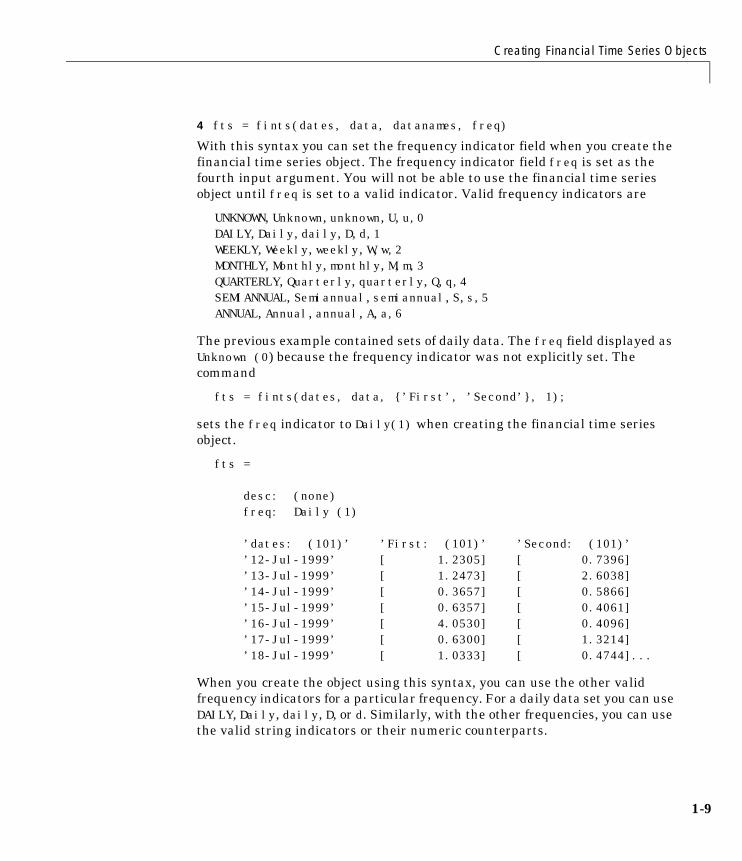
4 fts = fints(dates, data, datanames, freq)
With this syntax you can set the frequency indicator field when you create the financial time series object. The frequency indicator field freq is set as the fourth input argument. You will not be able to use the financial time series object until freq is set to a valid indicator. Valid frequency indicators are
UNKNOWN, Unknown, unknown, U, u,0DAILY, Daily, daily, D, d,1 WEEKLY, Weekly, weekly, W, w,2 MONTHLY, Monthly, monthly, M, m,3 QUARTERLY, Quarterly, quarterly, Q, q,4 SEMIANNUAL, Semiannual, semiannual, S, s,5 ANNUAL, Annual, annual, A, a,6
The previous example contained sets of daily data. The freq field displayed as Unknown (0) because the frequency indicator was not explicitly set. The command
fts = fints(dates, data, {’First’, ’Second’}, 1);
sets the freq indicator to Daily(1) when creating the financial time series object.
fts =
desc: (none)freq: Daily (1)
’dates: (101)’ ’First: (101)’ ’Second: (101)’’12-Jul-1999’ [ 1.2305] [ 0.7396]’13-Jul-1999’ [ 1.2473] [ 2.6038]’14-Jul-1999’ [ 0.3657] [ 0.5866]’15-Jul-1999’ [ 0.6357] [ 0.4061]’16-Jul-1999’ [ 4.0530] [ 0.4096]’17-Jul-1999’ [ 0.6300] [ 1.3214]’18-Jul-1999’ [ 1.0333] [ 0.4744]...
When you create the object using this syntax, you can use the other valid frequency indicators for a particular frequency. For a daily data set you can use DAILY, Daily, daily, D, or d. Similarly, with the other frequencies, you can use the valid string indicators or their numeric counterparts.
1-9
1 Tutorial
1-1
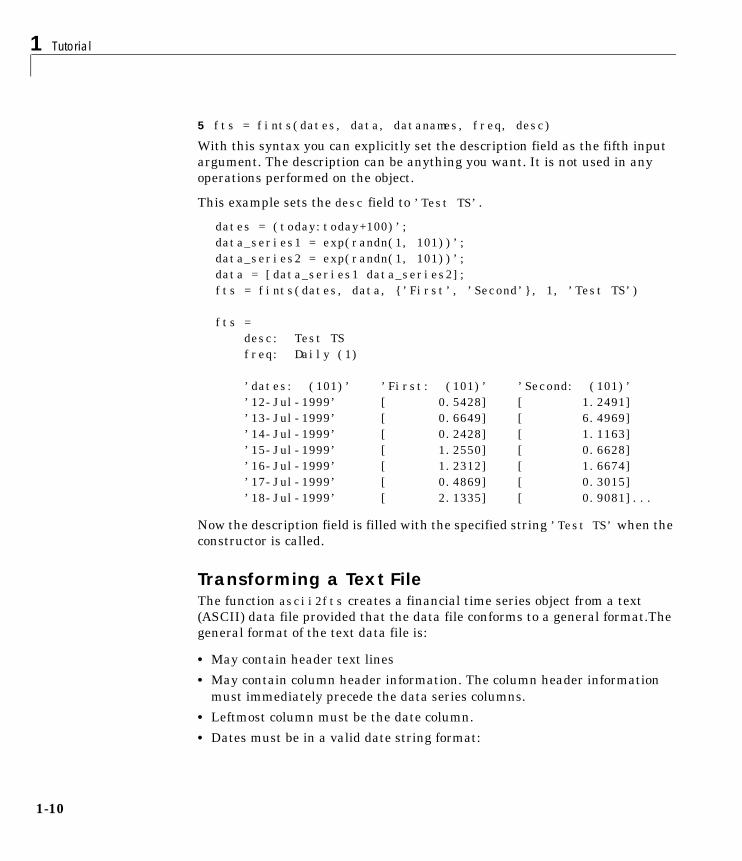
5 fts = fints(dates, data, datanames, freq, desc)
With this syntax you can explicitly set the description field as the fifth input argument. The description can be anything you want. It is not used in any operations performed on the object.
This example sets the desc field to ’Test TS’.
dates = (today:today+100)’;data_series1 = exp(randn(1, 101))’;data_series2 = exp(randn(1, 101))’;data = [data_series1 data_series2];fts = fints(dates, data, {’First’, ’Second’}, 1, ’Test TS’)
fts = desc: Test TSfreq: Daily (1)
’dates: (101)’ ’First: (101)’ ’Second: (101)’’12-Jul-1999’ [ 0.5428] [ 1.2491]’13-Jul-1999’ [ 0.6649] [ 6.4969]’14-Jul-1999’ [ 0.2428] [ 1.1163]’15-Jul-1999’ [ 1.2550] [ 0.6628]’16-Jul-1999’ [ 1.2312] [ 1.6674]’17-Jul-1999’ [ 0.4869] [ 0.3015]’18-Jul-1999’ [ 2.1335] [ 0.9081]...
Now the description field is filled with the specified string ’Test TS’ when the constructor is called.
Transforming a Text FileThe function ascii2fts creates a financial time series object from a text (ASCII) data file provided that the data file conforms to a general format.The general format of the text data file is:
• May contain header text lines
• May contain column header information. The column header information must immediately precede the data series columns.
• Leftmost column must be the date column.
• Dates must be in a valid date string format:
0
Creating Financial Time Series Objects
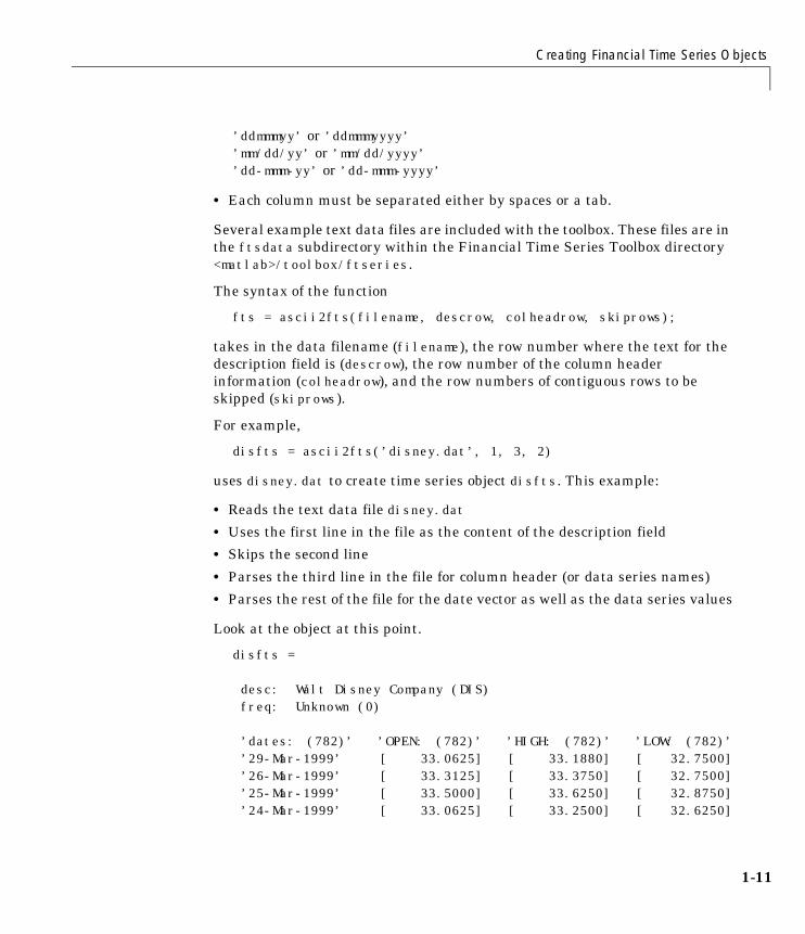
’ddmmmyy’ or ’ddmmmyyyy’’mm/dd/yy’ or ’mm/dd/yyyy’’dd-mmm-yy’ or ’dd-mmm-yyyy’
• Each column must be separated either by spaces or a tab.
Several example text data files are included with the toolbox. These files are in the ftsdata subdirectory within the Financial Time Series Toolbox directory <matlab>/toolbox/ftseries.
The syntax of the function
fts = ascii2fts(filename, descrow, colheadrow, skiprows);
takes in the data filename (filename), the row number where the text for the description field is (descrow), the row number of the column header information (colheadrow), and the row numbers of contiguous rows to be skipped (skiprows).
For example,
disfts = ascii2fts(’disney.dat’, 1, 3, 2)
uses disney.dat to create time series object disfts. This example:
• Reads the text data file disney.dat
• Uses the first line in the file as the content of the description field
• Skips the second line
• Parses the third line in the file for column header (or data series names)
• Parses the rest of the file for the date vector as well as the data series values
Look at the object at this point.
disfts =
desc: Walt Disney Company (DIS)freq: Unknown (0)
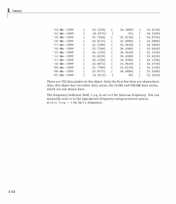
’dates: (782)’ ’OPEN: (782)’ ’HIGH: (782)’ ’LOW: (782)’’29-Mar-1999’ [ 33.0625] [ 33.1880] [ 32.7500]’26-Mar-1999’ [ 33.3125] [ 33.3750] [ 32.7500]’25-Mar-1999’ [ 33.5000] [ 33.6250] [ 32.8750]’24-Mar-1999’ [ 33.0625] [ 33.2500] [ 32.6250]
1-11
1 Tutorial
1-1
’23-Mar-1999’ [ 34.1250] [ 34.1880] [ 32.8130]’22-Mar-1999’ [ 34.9375] [ 35] [ 34.2500]’19-Mar-1999’ [ 35.7500] [ 35.8130] [ 34.8750]’18-Mar-1999’ [ 34.8125] [ 35.6880] [ 34.6880]’17-Mar-1999’ [ 35.2500] [ 35.5630] [ 34.5000]’16-Mar-1999’ [ 35.7500] [ 36.4380] [ 35.0630]’15-Mar-1999’ [ 36.1250] [ 36.5630] [ 35.1250]’12-Mar-1999’ [ 35.6250] [ 36.4380] [ 35.6250]’11-Mar-1999’ [ 34.1250] [ 34.9380] [ 34.1250]’10-Mar-1999’ [ 34.6875] [ 35.0630] [ 34.3750]’09-Mar-1999’ [ 35.7500] [ 35.8130] [ 34.3130]’08-Mar-1999’ [ 35.9375] [ 36.6880] [ 35.9380]’05-Mar-1999’ [ 35.8125] [ 36] [ 35.5630]
There are 782 data points in this object. Only the first few lines are shown here. Also, this object has two other data series, the CLOSE and VOLUME data series, which are not shown here.
The frequency indicator field, freq, is set to 0 for Unknown frequency. You can manually reset it to the appropriate frequency using structure syntax, disfts.freq = 1 for Daily frequency.
2

Working with Financial Time Series Objects
Working with Financial Time Series ObjectsA financial time series object is designed to be used as if it were a MATLAB structure. (See the MATLAB documentation for a description of MATLAB structures or how to use MATLAB in general.)
This part of the tutorial assumes that you know how to use MATLAB and are familiar with MATLAB structures. The terminology is similar to that of a MATLAB structure. The financial time series object term component is interchangeable with the MATLAB structure term field.
Financial Time Series Object StructureA financial time series object always contains three component names: desc (description field), freq (frequency indicator field), and dates (date vector). If you build the object using the constructor fints, the default value for the description field is a blank string (’’). If you build the object from a text data file using ascii2fts, the default is the name of the text data file. The default for the frequency indicator field is 0 (Unknown frequency). Objects created from operations may default the setting to 0; for example, if you decide to selectively pick out values from an object, the frequency of the new object may not be the same as that of object from which it came.
The date vector dates does not have a default set of values. When you create an object, you have to supply the date vector. You can change the date vector afterwards but, at object creation time, you must provide a set of dates.
The final component of a financial time series object is one or more data series vectors. If you do not supply a name for the data series, the default name is series1. If you have multiple data series in an object and do not supply the names, the default is the name series followed by a number, for example, series1, series2, and series3.
Data ExtractionHere is an exercise on how to extract data from a financial time series object. As mentioned before, you can think of the object as a MATLAB structure. Cut and paste each line in the exercise to the MATLAB command window and press Enter to execute it.
To begin create a financial time series object called myfts.
1-13

1 Tutorial
1-1
dates = (datenum(’05/11/99’):datenum(’05/11/99’)+100)’;data_series1 = exp(randn(1, 101))’;data_series2 = exp(randn(1, 101))’;data = [data_series1 data_series2];myfts = fints(dates, data);
The myfts object looks like
myfts =
desc: (none)freq: Unknown (0)
’dates: (101)’ ’series1: (101)’ ’series2: (101)’’11-May-1999’ [ 2.8108] [ 0.9323]’12-May-1999’ [ 0.2454] [ 0.5608]’13-May-1999’ [ 0.3568] [ 1.5989]’14-May-1999’ [ 0.5255] [ 3.6682]’15-May-1999’ [ 1.1862] [ 5.1284]’16-May-1999’ [ 3.8376] [ 0.4952]’17-May-1999’ [ 6.9329] [ 2.2417]’18-May-1999’ [ 2.0987] [ 0.3579]’19-May-1999’ [ 2.2524] [ 3.6492]’20-May-1999’ [ 0.8669] [ 1.0150]’21-May-1999’ [ 0.9050] [ 1.2445]’22-May-1999’ [ 0.4493] [ 5.5466]’23-May-1999’ [ 1.6376] [ 0.1251]’24-May-1999’ [ 3.4472] [ 1.1195]’25-May-1999’ [ 3.6545] [ 0.3374]...
There are more dates in the object; only the first few lines are shown here.
Now create another object with only the values for series2.
srs2 = myfts.series2
srs2 =
desc: (none)freq: Unknown (0)
’dates: (101)’ ’series2: (101)’
4

Working with Financial Time Series Objects
’11-May-1999’ [ 0.9323]’12-May-1999’ [ 0.5608]’13-May-1999’ [ 1.5989]’14-May-1999’ [ 3.6682]’15-May-1999’ [ 5.1284]’16-May-1999’ [ 0.4952]’17-May-1999’ [ 2.2417]’18-May-1999’ [ 0.3579]’19-May-1999’ [ 3.6492]’20-May-1999’ [ 1.0150]’21-May-1999’ [ 1.2445]’22-May-1999’ [ 5.5466]’23-May-1999’ [ 0.1251]’24-May-1999’ [ 1.1195]’25-May-1999’ [ 0.3374]...
The new object srs2 contains all the dates in myfts, but the data series is only series2. The name of the data series retains its name from the original object, myfts.
Note The output from referencing a data series field or indexing a financial time series object is always another financial time series object. The exceptions are referencing the description, frequency indicator, and dates fields, and indexing into the dates field.
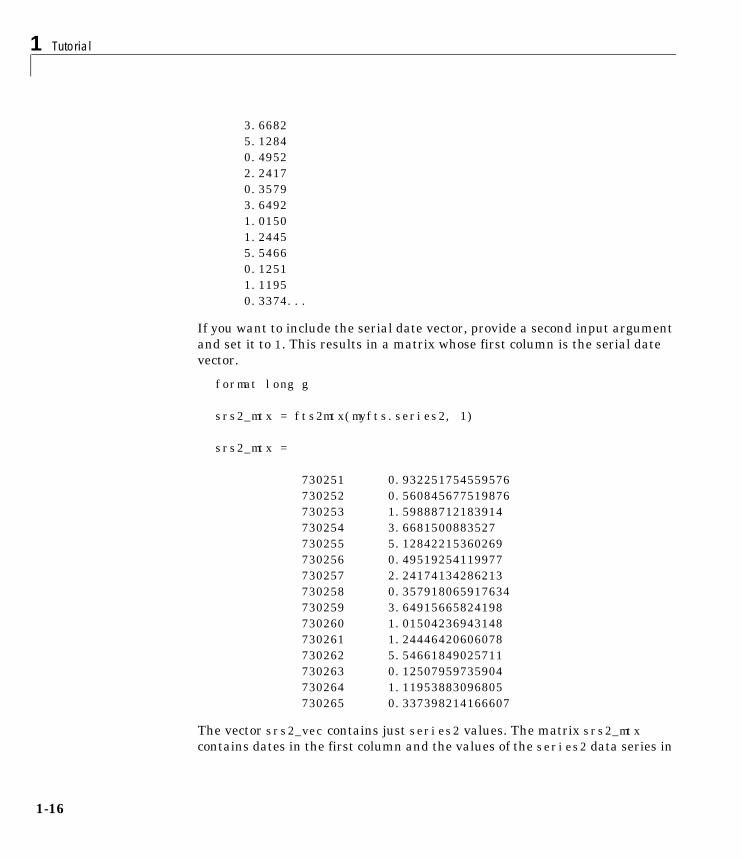
Object to Matrix ConversionThe function fts2mtx extracts the dates and/or the data series values from an object and places them into a vector or a matrix. The default behavior extracts just the values into a vector or a matrix. Look at the next example.
srs2_vec = fts2mtx(myfts.series2)
srs2_vec =
0.93230.56081.5989
1-15
1 Tutorial
1-1
3.66825.12840.49522.24170.35793.64921.01501.24455.54660.12511.11950.3374...
If you want to include the serial date vector, provide a second input argument and set it to 1. This results in a matrix whose first column is the serial date vector.
format long g
srs2_mtx = fts2mtx(myfts.series2, 1)
srs2_mtx =
730251 0.932251754559576730252 0.560845677519876730253 1.59888712183914730254 3.6681500883527730255 5.12842215360269730256 0.49519254119977730257 2.24174134286213730258 0.357918065917634730259 3.64915665824198730260 1.01504236943148730261 1.24446420606078730262 5.54661849025711730263 0.12507959735904730264 1.11953883096805730265 0.337398214166607
The vector srs2_vec contains just series2 values. The matrix srs2_mtx contains dates in the first column and the values of the series2 data series in
6

Working with Financial Time Series Objects
the second. Dates in the first column are in serial date format. Serial date format is a representation of the date string format (for example, serial date = 1 is equivalent to 01-Jan-0000). The long g display format displays the numbers without exponentiation. (To revert to the default display format, use format short. See the format command in the MATLAB documentation for a description of MATLAB display formats.) Remember that both the vector and the matrix have 101 rows of data as in the original object myfts but are shown truncated here.
Indexing a Financial Time Series ObjectYou can also index into the object as with any other MATLAB variable or structure. A financial time series object lets you use a date string, a cell array of date strings, a date string range, or normal integer indexing. You cannot, however, index into the object using serial dates. If you have serial dates, you must first use the MATLAB datestr command to convert them into date strings.
When indexing by date string note that:
• Each date string must contain the day, month, and year. Valid formats are:
- ’mm/dd/yy’ or ’mm/dd/yyyy’
- ’dd-mmm-yy’ or ’dd-mmm-yyyy’
- ’mmm dd, yy’ or ’mmm dd, yyyy’
• All data falls at the end of indicated time period, that is, weekly data falls on Fridays, monthly data falls on the end of each month, etc., whenever the data has gone through a frequency conversion.
Indexing with Date StringsWith date string indexing you get the values in a financial time series object for a specific date using a date string as the index into the object. Similarly, if you want values for multiple dates in the object, you can put those date strings into a cell array and use the cell array as the index to the object. Here are some examples.
This example extracts all values for May 11, 1999 from myfts.
format shortmyfts(’05/11/99’)
1-17

1 Tutorial
1-1
ans =
desc: (none)freq: Unknown (0)
’dates: (1)’ ’series1: (1)’ ’series2: (1)’’11-May-1999’ [ 2.8108] [ 0.9323]
The next example extracts only series2 values for May 11, 1999 from myfts.
myfts.series2(’05/11/99’)
ans =
desc: (none)freq: Unknown (0)
’dates: (1)’ ’series2: (1)’’11-May-1999’ [ 0.9323]
The third example extracts all values for three different dates.
myfts({’05/11/99’, ’05/21/99’, ’05/31/99’})
ans =
desc: (none)freq: Unknown (0)
’dates: (3)’ ’series1: (3)’ ’series2: (3)’’11-May-1999’ [ 2.8108] [ 0.9323]’21-May-1999’ [ 0.9050] [ 1.2445]’31-May-1999’ [ 1.4266] [ 0.6470]
The next extracts only series2 values for the same three dates.
myfts.series2({’05/11/99’, ’05/21/99’, ’05/31/99’})
ans =
desc: (none)freq: Unknown (0)
8

Working with Financial Time Series Objects
’dates: (3)’ ’series2: (3)’’11-May-1999’ [ 0.9323]’21-May-1999’ [ 1.2445]’31-May-1999’ [ 0.6470]
Indexing with Date String RangeA financial time series is unique because it allows you to index the object using a date string range. A date string range consists of two date strings separated by two colons (::). In MATLAB this separator is called the double-colon operator. An example of a MATLAB date string range is ’05/11/99::05/31/99’. The operator gives you all data points available between those dates, including the start and end dates.
Here are some date string range examples.
myfts (’05/11/99::05/15/99’)
ans =
desc: (none)freq: Unknown (0)
’dates: (5)’ ’series1: (5)’ ’series2: (5)’’11-May-1999’ [ 2.8108] [ 0.9323]’12-May-1999’ [ 0.2454] [ 0.5608]’13-May-1999’ [ 0.3568] [ 1.5989]’14-May-1999’ [ 0.5255] [ 3.6682]’15-May-1999’ [ 1.1862] [ 5.1284]
myfts.series2(’05/11/99::05/15/99’)
ans =
desc: (none)freq: Unknown (0)
’dates: (5)’ ’series2: (5)’’11-May-1999’ [ 0.9323]’12-May-1999’ [ 0.5608]
1-19
1 Tutorial
1-2
’13-May-1999’ [ 1.5989]’14-May-1999’ [ 3.6682]’15-May-1999’ [ 5.1284]
As with any other MATLAB variable or structure, you can assign the output to another object variable.
nfts = myfts.series2(’05/11/99::05/20/99’);
nfts is the same as ans in the second example.
If one of the dates does not exist in the object, an error message indicates that one or both date indexes are out of the range of the available dates in the object. You can either display the contents of the object or use the command ftsbound to determine the first and last dates in the object.
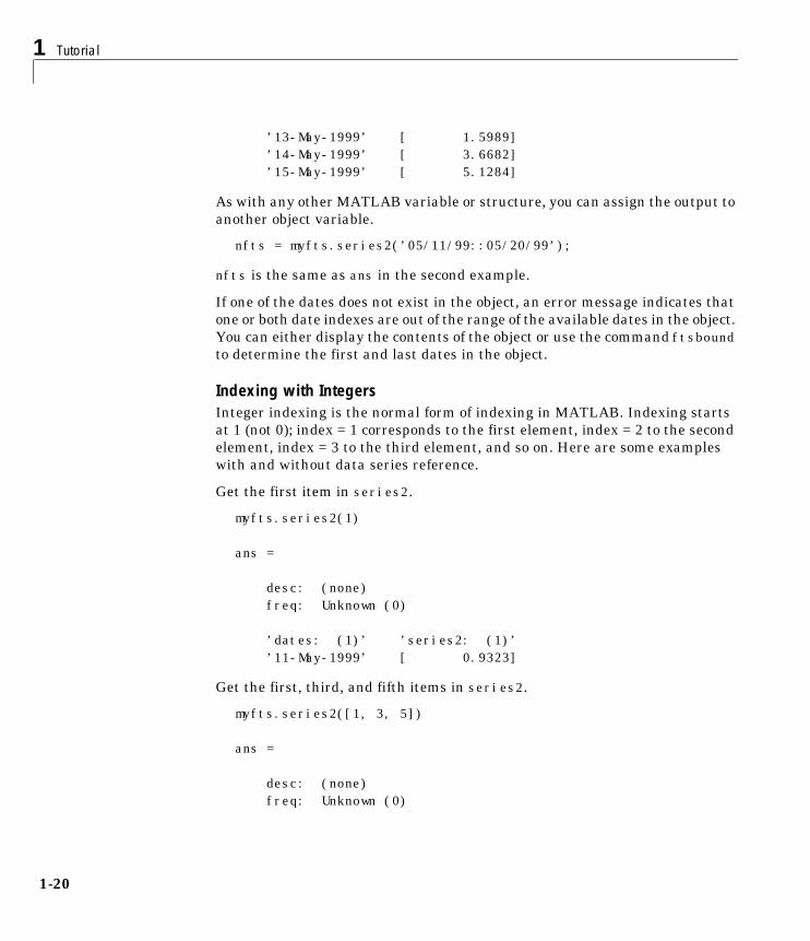
Indexing with IntegersInteger indexing is the normal form of indexing in MATLAB. Indexing starts at 1 (not 0); index = 1 corresponds to the first element, index = 2 to the second element, index = 3 to the third element, and so on. Here are some examples with and without data series reference.
Get the first item in series2.
myfts.series2(1)
ans =
desc: (none)freq: Unknown (0)
’dates: (1)’ ’series2: (1)’’11-May-1999’ [ 0.9323]
Get the first, third, and fifth items in series2.
myfts.series2([1, 3, 5])
ans =
desc: (none)freq: Unknown (0)
0
Working with Financial Time Series Objects
’dates: (3)’ ’series2: (3)’’11-May-1999’ [ 0.9323]’13-May-1999’ [ 1.5989]’15-May-1999’ [ 5.1284]
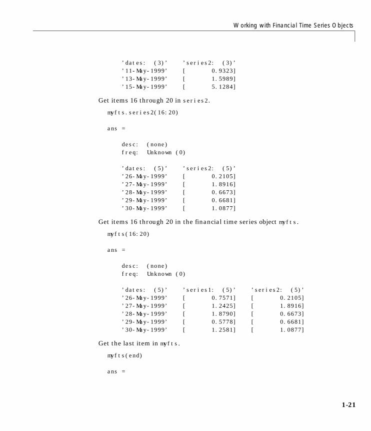
Get items 16 through 20 in series2.
myfts.series2(16:20)
ans =
desc: (none)freq: Unknown (0)
’dates: (5)’ ’series2: (5)’’26-May-1999’ [ 0.2105]’27-May-1999’ [ 1.8916]’28-May-1999’ [ 0.6673]’29-May-1999’ [ 0.6681]’30-May-1999’ [ 1.0877]
Get items 16 through 20 in the financial time series object myfts.
myfts(16:20)
ans =
desc: (none)freq: Unknown (0)
’dates: (5)’ ’series1: (5)’ ’series2: (5)’’26-May-1999’ [ 0.7571] [ 0.2105]’27-May-1999’ [ 1.2425] [ 1.8916]’28-May-1999’ [ 1.8790] [ 0.6673]’29-May-1999’ [ 0.5778] [ 0.6681]’30-May-1999’ [ 1.2581] [ 1.0877]
Get the last item in myfts.
myfts(end)
ans =
1-21
1 Tutorial
1-2
desc: (none)freq: Unknown (0)
’dates: (1)’ ’series1: (1)’ ’series2: (1)’’19-Aug-1999’ [ 1.4692] [ 3.4238]
The last example uses the MATLAB special variable end, which points to the last element of the object when used as an index. The example returns an object whose contents are the values in the object myfts on the last date entry.
OperationsSeveral MATLAB functions have been overloaded to work with financial time series objects. The overloaded functions include basic arithmetic functions such as addition, subtraction, multiplication, and division as well as other functions such as arithmetic average, filter, and difference. Also, specific methods have been designed to work with the financial time series object. For a list of functions grouped by type, refer to the “Functions by Category” or enter
help ftseries
at the MATLAB command prompt.
Basic ArithmeticFinancial time series objects permit you to do addition, subtraction, multiplication, and division, either on the entire object or on specific object fields. This is a feature that MATLAB structures do not allow. You cannot do arithmetic operations on entire MATLAB structures, only on specific fields of a structure.
You can perform arithmetic operations on two financial time series objects as long as they are compatible (all contents are the same except for the description and the values associated with the data series.)
Note Compatible time series are not the same as equal time series. Two time series objects are equal when everything but the description fields are the same.
2
Working with Financial Time Series Objects
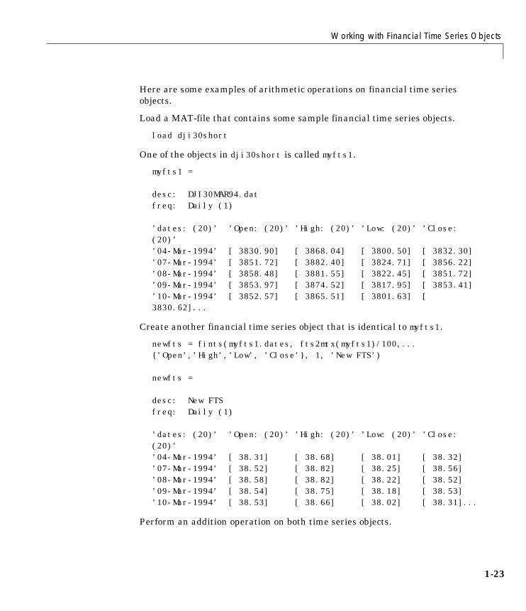
Here are some examples of arithmetic operations on financial time series objects.
Load a MAT-file that contains some sample financial time series objects.
load dji30short
One of the objects in dji30short is called myfts1.
myfts1 =
desc: DJI30MAR94.datfreq: Daily (1)
’dates: (20)’ ’Open: (20)’ ’High: (20)’ ’Low: (20)’ ’Close: (20)’’04-Mar-1994’ [ 3830.90] [ 3868.04] [ 3800.50] [ 3832.30]’07-Mar-1994’ [ 3851.72] [ 3882.40] [ 3824.71] [ 3856.22]’08-Mar-1994’ [ 3858.48] [ 3881.55] [ 3822.45] [ 3851.72]’09-Mar-1994’ [ 3853.97] [ 3874.52] [ 3817.95] [ 3853.41]’10-Mar-1994’ [ 3852.57] [ 3865.51] [ 3801.63] [ 3830.62]...
Create another financial time series object that is identical to myfts1.
newfts = fints(myfts1.dates, fts2mtx(myfts1)/100,... {’Open’,’High’,’Low’, ’Close’}, 1, ’New FTS’)
newfts =
desc: New FTSfreq: Daily (1)
’dates: (20)’ ’Open: (20)’ ’High: (20)’ ’Low: (20)’ ’Close: (20)’’04-Mar-1994’ [ 38.31] [ 38.68] [ 38.01] [ 38.32]’07-Mar-1994’ [ 38.52] [ 38.82] [ 38.25] [ 38.56]’08-Mar-1994’ [ 38.58] [ 38.82] [ 38.22] [ 38.52]’09-Mar-1994’ [ 38.54] [ 38.75] [ 38.18] [ 38.53]’10-Mar-1994’ [ 38.53] [ 38.66] [ 38.02] [ 38.31]...
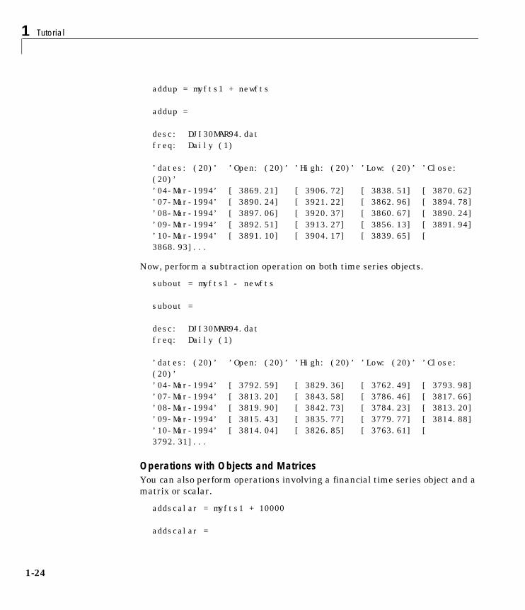
Perform an addition operation on both time series objects.
1-23
1 Tutorial
1-2
addup = myfts1 + newfts
addup =
desc: DJI30MAR94.datfreq: Daily (1)
’dates: (20)’ ’Open: (20)’ ’High: (20)’ ’Low: (20)’ ’Close: (20)’’04-Mar-1994’ [ 3869.21] [ 3906.72] [ 3838.51] [ 3870.62]’07-Mar-1994’ [ 3890.24] [ 3921.22] [ 3862.96] [ 3894.78]’08-Mar-1994’ [ 3897.06] [ 3920.37] [ 3860.67] [ 3890.24]’09-Mar-1994’ [ 3892.51] [ 3913.27] [ 3856.13] [ 3891.94]’10-Mar-1994’ [ 3891.10] [ 3904.17] [ 3839.65] [ 3868.93]...
Now, perform a subtraction operation on both time series objects.
subout = myfts1 - newfts
subout =
desc: DJI30MAR94.datfreq: Daily (1)
’dates: (20)’ ’Open: (20)’ ’High: (20)’ ’Low: (20)’ ’Close: (20)’’04-Mar-1994’ [ 3792.59] [ 3829.36] [ 3762.49] [ 3793.98]’07-Mar-1994’ [ 3813.20] [ 3843.58] [ 3786.46] [ 3817.66]’08-Mar-1994’ [ 3819.90] [ 3842.73] [ 3784.23] [ 3813.20]’09-Mar-1994’ [ 3815.43] [ 3835.77] [ 3779.77] [ 3814.88]’10-Mar-1994’ [ 3814.04] [ 3826.85] [ 3763.61] [ 3792.31]...
Operations with Objects and MatricesYou can also perform operations involving a financial time series object and a matrix or scalar.
addscalar = myfts1 + 10000
addscalar =
4
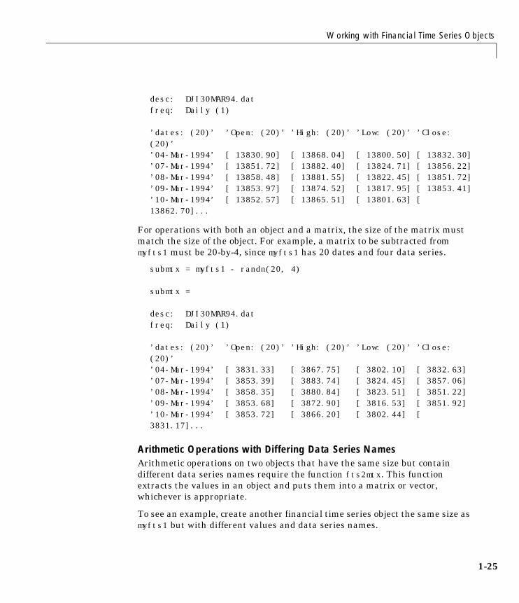
Working with Financial Time Series Objects
desc: DJI30MAR94.datfreq: Daily (1)
’dates: (20)’ ’Open: (20)’ ’High: (20)’ ’Low: (20)’ ’Close: (20)’’04-Mar-1994’ [ 13830.90] [ 13868.04] [ 13800.50] [ 13832.30]’07-Mar-1994’ [ 13851.72] [ 13882.40] [ 13824.71] [ 13856.22]’08-Mar-1994’ [ 13858.48] [ 13881.55] [ 13822.45] [ 13851.72]’09-Mar-1994’ [ 13853.97] [ 13874.52] [ 13817.95] [ 13853.41]’10-Mar-1994’ [ 13852.57] [ 13865.51] [ 13801.63] [ 13862.70]...
For operations with both an object and a matrix, the size of the matrix must match the size of the object. For example, a matrix to be subtracted from myfts1 must be 20-by-4, since myfts1 has 20 dates and four data series.
submtx = myfts1 - randn(20, 4)
submtx =
desc: DJI30MAR94.datfreq: Daily (1)
’dates: (20)’ ’Open: (20)’ ’High: (20)’ ’Low: (20)’ ’Close: (20)’’04-Mar-1994’ [ 3831.33] [ 3867.75] [ 3802.10] [ 3832.63]’07-Mar-1994’ [ 3853.39] [ 3883.74] [ 3824.45] [ 3857.06]’08-Mar-1994’ [ 3858.35] [ 3880.84] [ 3823.51] [ 3851.22]’09-Mar-1994’ [ 3853.68] [ 3872.90] [ 3816.53] [ 3851.92]’10-Mar-1994’ [ 3853.72] [ 3866.20] [ 3802.44] [ 3831.17]...
Arithmetic Operations with Differing Data Series NamesArithmetic operations on two objects that have the same size but contain different data series names require the function fts2mtx. This function extracts the values in an object and puts them into a matrix or vector, whichever is appropriate.
To see an example, create another financial time series object the same size as myfts1 but with different values and data series names.
1-25

1 Tutorial
1-2
newfts2 = fints(myfts1.dates, fts2mtx(myfts1)/10000),... {’Rat1’,’Rat2’, ’Rat3’,’Rat4’}, 1, ’New FTS’)
If you attempt to add (or subtract, etc.) this new object to myfts1, an error indicates that the objects are not identical. Although they contain the same dates, number of dates, number of data series, and frequency, the two time series objects do not have the same data series names. Use fts2mtx to bypass this problem.
addother = myfts1 + fts2mtx(newfts2);
This operation adds the matrix that contains the contents of the data series in the object newfts2 to myfts1. You should carefully consider the effects on your data before deciding to combine financial time series objects in this manner.
Other Arithmetic OperationsIn addition to the basic arithmetic operations, several other mathematical functions operate directly on financial time series objects. These functions include exponential (exp), natural logarithm (log), common logarithm (log10), and many more. See the “Function Reference” chapter for more details.
Data Transformation and Frequency ConversionThe data transformation and the frequency conversion functions convert a data series into a different format.
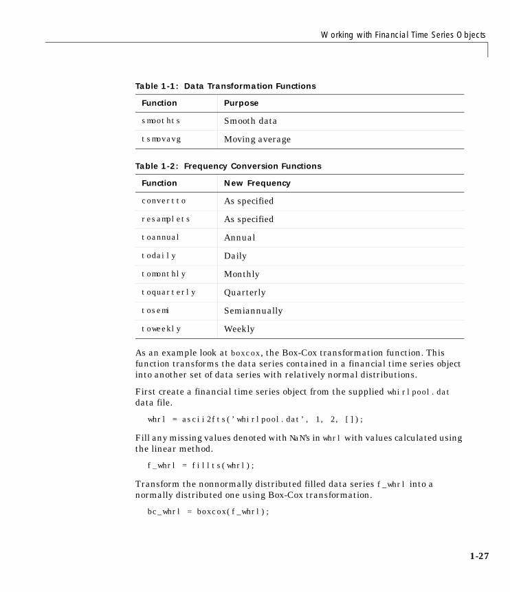
Table 1-1: Data Transformation Functions
Function Purpose
boxcox Box-Cox transformation
diff Differencing
fillts Fill missing values
filter Filter
lagts Lag time series object
leadts Lead time series object
peravg Periodic average
6
Working with Financial Time Series Objects
As an example look at boxcox, the Box-Cox transformation function. This function transforms the data series contained in a financial time series object into another set of data series with relatively normal distributions.
First create a financial time series object from the supplied whirlpool.dat data file.
whrl = ascii2fts(’whirlpool.dat’, 1, 2, []);
Fill any missing values denoted with NaN’s in whrl with values calculated using the linear method.
f_whrl = fillts(whrl);
Transform the nonnormally distributed filled data series f_whrl into a normally distributed one using Box-Cox transformation.
bc_whrl = boxcox(f_whrl);
smoothts Smooth data
tsmovavg Moving average
Table 1-2: Frequency Conversion Functions
Function New Frequency
convertto As specified
resamplets As specified
toannual Annual
todaily Daily
tomonthly Monthly
toquarterly Quarterly
tosemi Semiannually
toweekly Weekly
Table 1-1: Data Transformation Functions
Function Purpose
1-27

1 Tutorial
1-2
Compare the result of the Close data series with a normal (Gaussian) probability distribution function as well as the nonnormally distributed f_whrl.
subplot(2, 1, 1);hist(f_whrl.Close);grid; title(’Non-normally Distributed Data’);subplot(2, 1, 2);hist(bc_whrl.Close);grid; title(’Box-Cox Transformed Data’);
Figure 1-1: Box-Cox Transformation
In Figure 1-1, Box-Cox Transformation the bar chart on the top represents the probability distribution function of the filled data series, f_whrl, which is the original data series whrl with the missing values interpolated using the linear method. The distribution is skewed towards the left (not normally distributed). The bar chart on the bottom is less skewed to the left. If you plot a Gaussian probability distribution function (PDF) with similar mean and standard deviation, the distribution of the transformed data is very close to normal (Gaussian).
40 45 50 55 60 65 70 750
50
100
150
200
250
300Non−normally Distributed Data
0.5966 0.5968 0.597 0.5972 0.59740
50
100
150
200
250
300
350Box−Cox Transformed Data
8

Working with Financial Time Series Objects
When you examine the contents of the resulting object bc_whrl, you find an identical object to the original object whrl but the contents are the transformed data series. If you have the Statistics Toolbox, you can generate a Gaussian PDF with mean and standard deviation equal to those of the transformed data series and plot it as an overlay to the second bar chart. You can see that it is an approximately normal distribution (Figure 1-2, Overlay of Gaussian PDF).
Figure 1-2: Overlay of Gaussian PDF
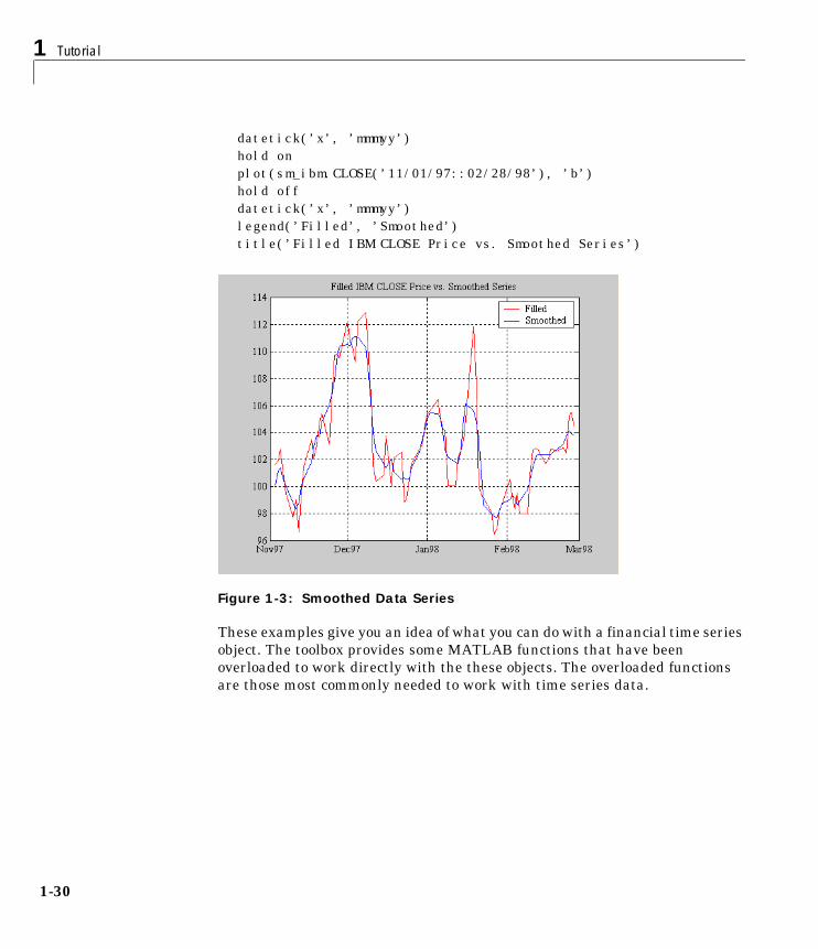
The next example uses the smoothts function to smooth a time series.
To begin, transform ibm9599.dat, a supplied data file, into a financial time series object.
ibm = ascii2fts(’ibm9599.dat’, 1, 3, 2);
Fill the holidays missing data with data interpolated using the fillts function and the Spline fill method.
f_ibm = fillts(ibm, ’Spline’);
Smooth the filled data series using the default Box (rectangular window) method.
sm_ibm = smoothts(f_ibm);
Now, plot the original and smoothed closing price series for IBM.
plot(f_ibm.CLOSE(’11/01/97::02/28/98’), ’r’)
1-29
1 Tutorial
1-3
datetick(’x’, ’mmmyy’)hold onplot(sm_ibm.CLOSE(’11/01/97::02/28/98’), ’b’)hold offdatetick(’x’, ’mmmyy’)legend(’Filled’, ’Smoothed’)title(’Filled IBM CLOSE Price vs. Smoothed Series’)
Figure 1-3: Smoothed Data Series
These examples give you an idea of what you can do with a financial time series object. The toolbox provides some MATLAB functions that have been overloaded to work directly with the these objects. The overloaded functions are those most commonly needed to work with time series data.
0
Technical Analysis
Technical AnalysisTechnical analysis (or charting) is used by some investment managers to help manage portfolios. Technical analysis relies heavily on the availability of historical data. Investment managers calculate different indicators from available data and plot them as charts. Observations of price, direction, and volume on the charts assist managers in making decisions on their investment portfolios.
The technical analysis functions in this toolbox are tools to help analyze your investments. The functions in themselves will not make any suggestions or perform any qualitative analysis of your investment.
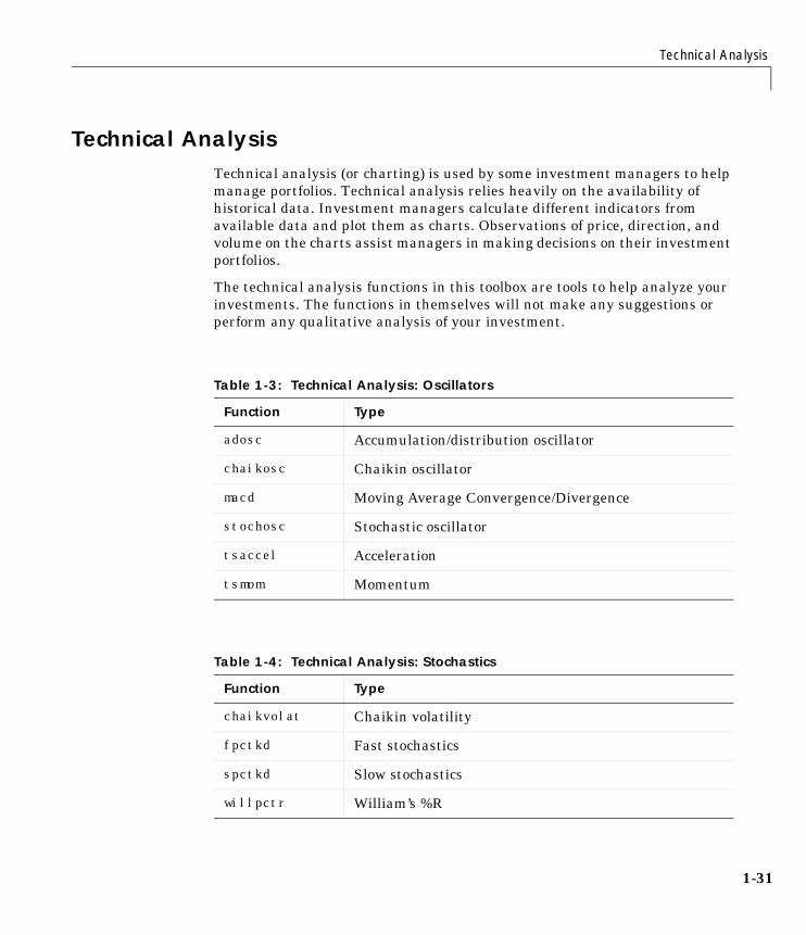
Table 1-3: Technical Analysis: Oscillators
Function Type
adosc Accumulation/distribution oscillator
chaikosc Chaikin oscillator
macd Moving Average Convergence/Divergence
stochosc Stochastic oscillator
tsaccel Acceleration
tsmom Momentum
Table 1-4: Technical Analysis: Stochastics
Function Type
chaikvolat Chaikin volatility
fpctkd Fast stochastics
spctkd Slow stochastics
willpctr William’s %R
1-31

1 Tutorial
1-3
Table 1-5: Technical Analysis: Indexes
Function Type
negvolidx Negative volume index
posvolidx Positive volume index
rsindex Relative strength index
Table 1-6: Technical Analysis: Indicators
Function Type
adline Accumulation/distribution line
bollinger Bollinger band
hhigh Highest high
llow Lowest low
medprice Median price
onbalvol On balance volume
prcroc Price rate of change
pvtrend Price-volume trend
typprice Typical price
volroc Volume rate of change
wclose Weighted close
willad William’s accumulation/distribution
2
Technical Analysis
ExamplesTo illustrate some the technical analysis functions, we will make use of the IBM stock price data contained in the supplied file ibm9599.dat. First create a financial time series object from the data using ascii2fts.
ibm = ascii2fts(’ibm9599.dat’, 1, 3, 2);
The time series data contains the open, close, high, and low prices, as well as the volume traded on each day. The time series dates start on January 3, 1995 and end on April 1, 1999 with some values missing for weekday holidays; weekend dates are not included.
Moving Average Convergence/Divergence (MACD)Moving Average Convergence/Divergence (MACD) is an oscillator function used by technical analysts to spot overbought and oversold conditions. Look at the portion of the time series covering the three-month period between October 1, 1995 to December 31, 1995. At the same time fill any missing values due to holidays within the time period specified.
part_ibm = fillts(ibm(’10/01/95::12/31/95’));
Now calculate the MACD, which when plotted produces two lines; the first line is the MACD line itself and the second is the nine-period moving average line.
macd_ibm = macd(part_ibm);
Note When you call macd without giving it a second input argument to specify a particular data series name, it searches for a closing price series named Close (in all combinations of letter cases). For more detail on the macd function, see macd in the “Function Reference”.
Plot the MACD lines and the High-Low plot of the IBM stock prices in two separate plots in one window.
subplot(2, 1, 1);plot(macd_ibm);title(’MACD of IBM Close Stock Prices, 10/01/95-12/31/95’);datetick(’x’, ’mm/dd/yy’);subplot(2, 1, 2);
1-33

1 Tutorial
1-3
highlow(part_ibm);title(’IBM Stock Prices, 10/01/95-12/31/95’);datetick(’x’, ’mm/dd/yy’)
Figure 1-4, MACD and IBM Stock Prices shows the result.
Figure 1-4: MACD and IBM Stock Prices
William’s %RWilliams %R is an indicator that measures overbought and oversold levels. The function willpctr is from the stochastics category. All the technical analysis functions can accept a different name for a required data series. If, for example, a function needs the high, low, and closing price series but your time series object does not have the data series names exactly as High, Low, and Close, you can specify the correct names as follows:
wpr = willpctr(tsobj, 14, 'HighName’, 'Hi', 'LowName', 'Lo',... 'CloseName', 'Closing')
The function willpctr now assumes that your high price series is named Hi, low price series is named Lo, and closing price series is named Closing.
4
Technical Analysis
Since the time series object part_ibm has its data series names identical to the required names, name adjustments are not needed. The input argument to the function is only the name of the time series object itself.
Calculate and plot the William’s %R indicator for IBM along with the price range using these commands.
wpctr_ibm = willpctr(part_ibm);subplot(2, 1, 1);plot(wpctr_ibm);title(’William’’s %R of IBM stock, 10/01/95-12/31/95’);datetick(’x’, ’mm/dd/yy’);hold on;plot(wpctr_ibm.dates, -80*ones(1, length(wpctr_ibm)),... ’color’, [0.5 0 0], ’linewidth’, 2)plot(wpctr_ibm.dates, -20*ones(1, length(wpctr_ibm)),...’color’, [0 0.5 0], ’linewidth’, 2)subplot(2, 1, 2);highlow(part_ibm);title(’IBM Stock Prices, 10/01/95-12/31/95’);datetick(’x’, ’mm/dd/yy’);
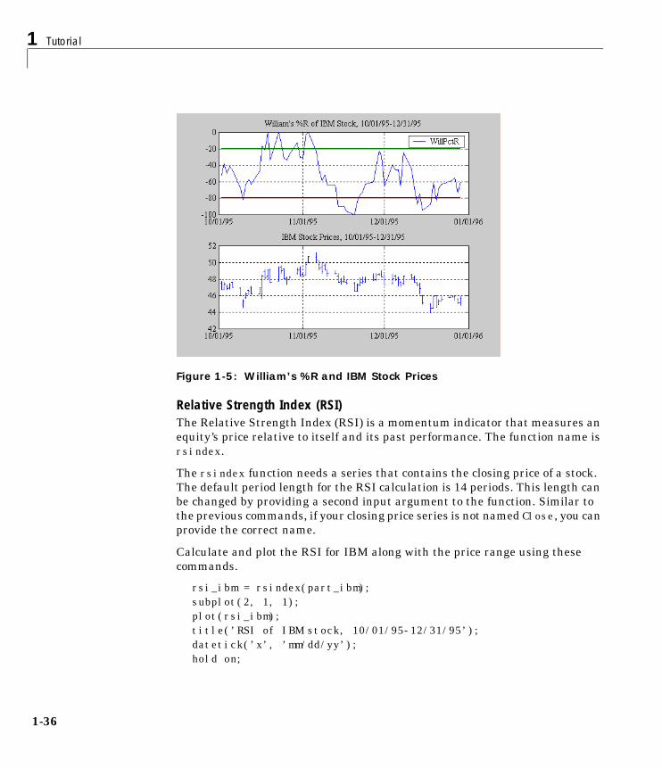
Figure 1-5, William’s %R and IBM Stock Prices shows the results. The top plot has the William's %R line plus two lines at -20% and -80%. The bottom plot is the High-Low plot of the IBM stock price for the corresponding time period.
1-35
1 Tutorial
1-3
Figure 1-5: William’s %R and IBM Stock Prices
Relative Strength Index (RSI)The Relative Strength Index (RSI) is a momentum indicator that measures an equity’s price relative to itself and its past performance. The function name is rsindex.
The rsindex function needs a series that contains the closing price of a stock. The default period length for the RSI calculation is 14 periods. This length can be changed by providing a second input argument to the function. Similar to the previous commands, if your closing price series is not named Close, you can provide the correct name.
Calculate and plot the RSI for IBM along with the price range using these commands.
rsi_ibm = rsindex(part_ibm);subplot(2, 1, 1);plot(rsi_ibm);title(’RSI of IBM stock, 10/01/95-12/31/95’);datetick(’x’, ’mm/dd/yy’);hold on;
6
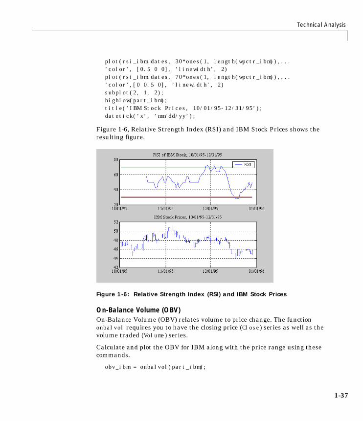
Technical Analysis
plot(rsi_ibm.dates, 30*ones(1, length(wpctr_ibm)),...’color’, [0.5 0 0], ’linewidth’, 2)plot(rsi_ibm.dates, 70*ones(1, length(wpctr_ibm)),... ’color’,[0 0.5 0], ’linewidth’, 2)subplot(2, 1, 2);highlow(part_ibm);title(’IBM Stock Prices, 10/01/95-12/31/95’);datetick(’x’, ’mm/dd/yy’);
Figure 1-6, Relative Strength Index (RSI) and IBM Stock Prices shows the resulting figure.
Figure 1-6: Relative Strength Index (RSI) and IBM Stock Prices
On-Balance Volume (OBV)On-Balance Volume (OBV) relates volume to price change. The function onbalvol requires you to have the closing price (Close) series as well as the volume traded (Volume) series.
Calculate and plot the OBV for IBM along with the price range using these commands.
obv_ibm = onbalvol(part_ibm);
1-37

1 Tutorial
1-3
subplot(2, 1, 1);plot(obv_ibm);title(’On-Balance Volume of IBM Stock, 10/01/95-12/31/95’);datetick(’x’, ’mm/dd/yy’);subplot(2, 1, 2);highlow(part_ibm);title(’IBM Stock Prices, 10/01/95-12/31/95’);datetick(’x’, ’mm/dd/yy’);
Figure 1-7, On-Balance Volume (OBV) and IBM Stock Prices shows the result.
Figure 1-7: On-Balance Volume (OBV) and IBM Stock Prices
8
Demonstration Program
Demonstration ProgramThis example demonstrates a practical use of the Financial Time Series Toolbox, predicting the return of a stock from a given set of data. The data is a series of closing stock prices, a series of dividend payments from the stock, and an explanatory series (in this case a market index). Additionally, the example calculates the dividend rate from the stock data provided.
Note You can find a script M-file for this demonstration program in the directory <matlab>/toolbox/ftseries/ftsdemos on your MATLAB path. The script is named predict_ret.m.
The series of steps needed to perform these computations is:
1 Load the data.
2 Create financial time series objects from the loaded data.
3 Create the series from dividend payment for adjusting the closing prices.
4 Adjust the closing prices and make them the spot prices.
5 Create the return series.
6 Regress the return series against the metric data (e.g., a market index) using the MATLAB \ operator.
7 Plot the results.
8 Calculate the dividend rate.
Load the DataThe data for this demonstration is found in the MAT-file predict_ret_data.mat.
load predict_ret_data.mat
The MAT-file contains six vectors:
1-39
1 Tutorial
1-4
• Dates corresponding to the closing stock prices, sdates
• Closing stock prices, sdata
• Dividend dates, divdates
• Dividend paid, divdata
• Dates corresponding to the metric data, expdates
• Metric data, expdata
Use the whos command to see the variables in your MATLAB workspace.
Create Financial Time Series Objects It is advantageous to work with financial time series objects rather than with the vectors now in the workspace. By using objects, you can easily keep track of the dates. Also, you can easily manipulate the data series based on dates because the object keeps track of the administration of time series for you.
Use the object constructor fints to construct three financial time series objects.
t0 = fints(sdates, sdata, {’Close’}, ’d’, ’Inc’);d0 = fints(divdates, divdata, {’Dividends’}, ’u’, ’Inc’);x0 = fints(expdates, expdata, {’Metric’}, ’w’, ’Index’);
The variables t0, d0, and x0, are financial time series objects containing the stock closing prices, dividend payments, and the explanatory data, respectively. To see the contents of an object, type its name at the MATLAB command prompt and press Enter. For example:
d0
d0 = ’desc:’ ’Inc’
’freq:’ ’Unknown (0)’ ’’ ’’ ’dates: (4)’ ’Dividends: (4)’ ’04/15/99’ ’0.2000’ ’06/30/99’ ’0.3500’ ’10/02/99’ ’0.2000’ ’12/30/99’ ’0.1500’
0
Demonstration Program
Create Closing Prices Adjustment SeriesThe price of a stock price is affected by the dividend payment. On the day before the dividend payment date, the stock price reflects the amount of dividend to be paid the next day. On the dividend payment date, the stock price is decreased by the amount of dividend paid. It is necessary to create a time series that reflects this adjustment factor.
dadj1 = d0;dadj1.dates = dadj1.dates-1;
Now create the series that adjust the prices at the day of dividend payment; this is an adjustment of 0. You also need to add the previous dividend payment date since the stock price data reflect the period subsequent to that day; the previous dividend date was December 31, 1998.
dadj2 = d0;dadj2.Dividends = 0;dadj2 = fillts(dadj2,’linear’,’12/31/98’);dadj2(’12/31/98’) = 0;
Combining the two objects above gives us the data that we need to adjust the prices. However, since the stock price data is daily data and the effect of the dividend is linearly divided during the period, use the fillts function to make a daily time series from the adjustment data. Use the dates from the stock price data to make the dates of the adjustment the same.
dadj3 = [dadj1; dadj2];dadj3 = fillts(dadj3, ’linear’, t0.dates);
Adjust Closing Prices and Make Them Spot PricesThe stock price recorded already reflects the dividend effect. To obtain the “correct” price, subtract the dividend amount from the closing prices. Put the result inside the same object t0 with the data series name Spot.
To make sure that adjustments correspond, index into the adjustment series using the dates from the stock price series t0. Use the datestr command because t0.dates returns the dates in serial date format. Also, since the data series name in the adjustment series dadj3 does not match the one in t0, use the function fts2mtx.
t0.Spot = t0.Close - fts2mtx(dadj3(datestr(t0.dates)));
1-41
1 Tutorial
1-4
Create Return SeriesNow calculate the return series from the stock price data. A stock return is calculated by dividing the difference between the current closing price and the previous closing price by the previous closing price.
tret = (t0.Spot - lagts(t0.Spot, 1)) ./ lagts(t0.Spot, 1);tret = chfield(tret, ’Spot’, ’Return’);
Ignore any warnings you receive during this sequence. Since the operation on the first line above preserves the data series name Spot, it has to be changed with the chfield command to reflect the contents correctly.
Regress Return Series Against Metric DataThe explanatory (metric) data set is a weekly data set while the stock price data is a daily data set. The frequency needs to be the same. Use todaily to convert the weekly series into a daily series. The constant needs to be included here to get the constant factor from the regression.
x1 = todaily(x0);x1.Const = 1;
Get all the dates common to the return series calculated above and the explanatory (metric) data. Then combine the contents of the two series that have dates in both into a new time series.
dcommon = intersect(tret.dates, x1.dates);regts0 = [tret(datestr(dcommon)), x1(datestr(dcommon))];
Remove the contents of the new time series that are not finite.
finite_regts0 = find(all(isfinite( fts2mtx(regts0)), 2));regts1 = regts0( finite_regts0 );
Now, place the data to be regressed into a matrix using the function fts2mtx. The first column of the matrix corresponds to the values of the first data series in the object, the second column to the second data series, and so on. In this case, the first column is regressed against the second and third column.
DataMatrix = fts2mtx(regts1);XCoeff = DataMatrix(:, 2:3) \ DataMatrix(:, 1);
2

Demonstration Program
Using the regression coefficients, calculate the predicted return from the stock price data. Put the result into the return time series tret as the data series PredReturn.
RetPred = DataMatrix(:,2:3) * XCoeff;tret.PredReturn(datestr(regts1.dates)) = RetPred;
Plot the ResultsPlot the results in a single figure window. The top plot in the window has the actual closing stock prices and the dividend-adjusted stock prices (spot prices). The bottom plot shows the actual return of the stock and the predicted stock return through regression.
subplot(2, 1, 1);plot(t0);title(’Spot and Closing Prices of Stock’);subplot(2, 1, 2);plot(tret);title(’Actual and Predicted Return of Stock’);
Figure 1-8: Closing Prices and Returns
1-43
1 Tutorial
1-4
Calculate the Dividend RateThe last part of the task is to calculate the dividend rate from the stock price data. Calculate the dividend rate by dividing the dividend payments with the corresponding closing stock prices.
First check to see if you have the stock price data on all the dividend dates.
datestr(d0.dates, 2)
ans =
04/15/9906/30/9910/02/9912/30/99
t0(datestr(d0.dates))
ans = ’desc:’ ’Inc’ ’’ ’freq:’ ’Daily (1)’ ’’ ’’ ’’ ’’ ’dates: (3)’ ’Close: (3)’ ’Spot: (3)’ ’04/15/99’ ’10.3369’ ’10.3369’ ’06/30/99’ ’11.4707’ ’11.4707’ ’12/30/99’ ’11.2244’ ’11.2244’
Note that stock price data for October 2, 1999 does not exist. The fillts function can overcome this situation; fillts allows you to insert a date and interpolate a value for the date from the existing values in the series. There are a number of interpolation methods. See fillts in the “Function Reference” for details.
Use fillts to create a new time series containing the missing date from the original data series. Then set the frequency indicator to daily.
t1 = fillts(t0,’nearest’,d0.dates);t1.freq = ’d’;
Calculate the dividend rate.
tdr = d0./fts2mtx(t1.Close(datestr(d0.dates)))
4
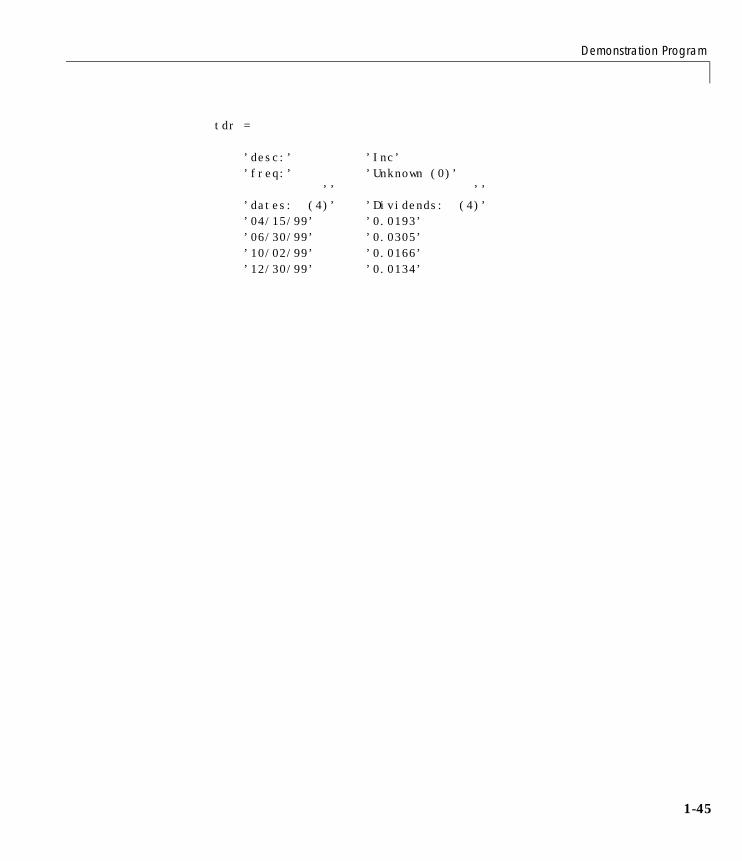
Demonstration Program
tdr = ’desc:’ ’Inc’ ’freq:’ ’Unknown (0)’ ’’ ’’ ’dates: (4)’ ’Dividends: (4)’ ’04/15/99’ ’0.0193’ ’06/30/99’ ’0.0305’ ’10/02/99’ ’0.0166’ ’12/30/99’ ’0.0134’
1-45

1 Tutorial
1-4
6
2
Function Reference
2 Function Reference
2-2
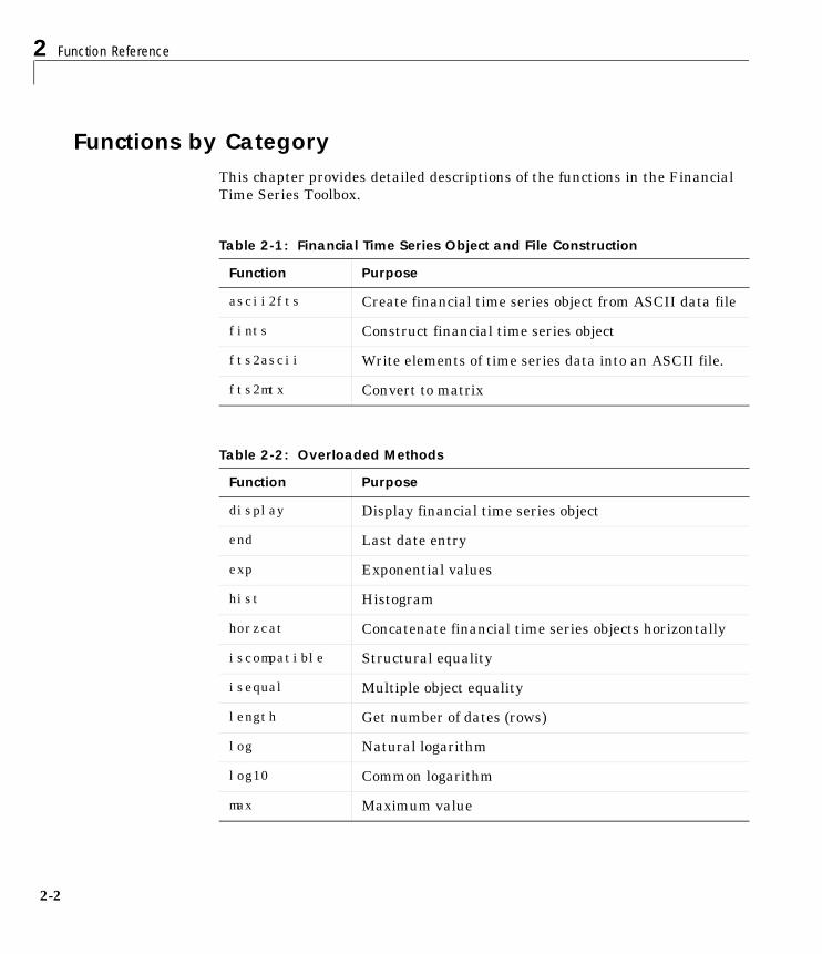
Functions by CategoryThis chapter provides detailed descriptions of the functions in the Financial Time Series Toolbox.
Table 2-1: Financial Time Series Object and File Construction
Function Purpose
ascii2fts Create financial time series object from ASCII data file
fints Construct financial time series object
fts2ascii Write elements of time series data into an ASCII file.
fts2mtx Convert to matrix
Table 2-2: Overloaded Methods
Function Purpose
display Display financial time series object
end Last date entry
exp Exponential values
hist Histogram
horzcat Concatenate financial time series objects horizontally
iscompatible Structural equality
isequal Multiple object equality
length Get number of dates (rows)
log Natural logarithm
log10 Common logarithm
max Maximum value

mean Arithmetic average
min Minimum value
minus Financial time series subtraction
mrdivide Financial time series matrix division
mtimes Financial time series matrix multiplication
plus Financial time series addition
power Financial time series power
rdivide Financial time series division
size Get number of dates and data series
sortfts Sort financial time series
std Standard deviation
subsasgn Content assignment
subsref Subscripted reference
times Financial time series multiplication
uminus Unary minus of financial time series object
uplus Unary plus of financial time series object
vertcat Concatenate financial time series objects vertically
Table 2-3: Utility Functions
Function Purpose
chfield Change data series name
extfield Extract data series
Table 2-2: Overloaded Methods (Continued)
Function Purpose
2-3

2 Function Reference
2-4
fieldnames Get names of fields
freqnum Convert string frequency indicator to numeric frequency indicator
freqstr Convert numeric frequency indicator to string representation
ftsbound Start and end dates
getfield Get content of a specific field
getnameidx Find name in list
isfield Check if a string is a field name
rmfield Remove data series
setfield Set content of a specific field
Table 2-4: Data Transformation Functions
Function Purpose
boxcox Box-Cox transformation
convertto Convert to specified frequency
demts2fts Convert demonstration time series to financial time series object
diff Differencing
fillts Fill missing values in time series
filter Linear filtering
lagts Lag time series object
leadts Lead time series object
Table 2-3: Utility Functions (Continued)
Function Purpose
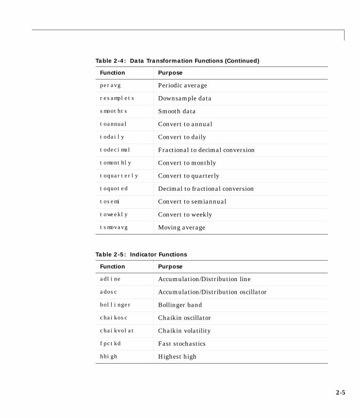
peravg Periodic average
resamplets Downsample data
smoothts Smooth data
toannual Convert to annual
todaily Convert to daily
todecimal Fractional to decimal conversion
tomonthly Convert to monthly
toquarterly Convert to quarterly
toquoted Decimal to fractional conversion
tosemi Convert to semiannual
toweekly Convert to weekly
tsmovavg Moving average
Table 2-5: Indicator Functions
Function Purpose
adline Accumulation/Distribution line
adosc Accumulation/Distribution oscillator
bollinger Bollinger band
chaikosc Chaikin oscillator
chaikvolat Chaikin volatility
fpctkd Fast stochastics
hhigh Highest high
Table 2-4: Data Transformation Functions (Continued)
Function Purpose
2-5
2 Function Reference
2-6
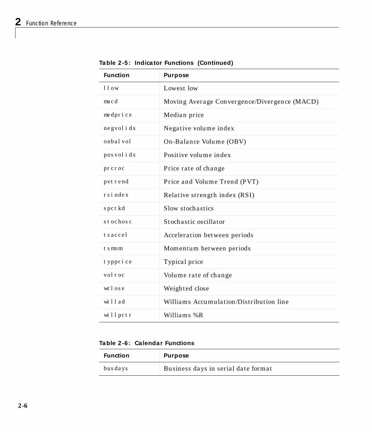
llow Lowest low
macd Moving Average Convergence/Divergence (MACD)
medprice Median price
negvolidx Negative volume index
onbalvol On-Balance Volume (OBV)
posvolidx Positive volume index
prcroc Price rate of change
pvtrend Price and Volume Trend (PVT)
rsindex Relative strength index (RSI)
spctkd Slow stochastics
stochosc Stochastic oscillator
tsaccel Acceleration between periods
tsmom Momentum between periods
typprice Typical price
volroc Volume rate of change
wclose Weighted close
willad Williams Accumulation/Distribution line
willpctr Williams %R
Table 2-6: Calendar Functions
Function Purpose
busdays Business days in serial date format
Table 2-5: Indicator Functions (Continued)
Function Purpose

Table 2-7: Plotting Functions
Function Purpose
candle Candle plot
chartfts Interactive display
highlow High-Low plot
plot Plot data series
2-7

2 Function Reference
2-8
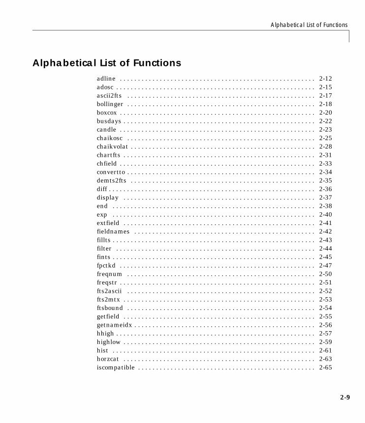
Alphabetical List of Functions
Alphabetical List of Functions 2
adline . . . . . . . . . . . . . . . . . . . . . . . . . . . . . . . . . . . . . . . . . . . . . . . . . . . . . . 2-12adosc . . . . . . . . . . . . . . . . . . . . . . . . . . . . . . . . . . . . . . . . . . . . . . . . . . . . . . . 2-15ascii2fts . . . . . . . . . . . . . . . . . . . . . . . . . . . . . . . . . . . . . . . . . . . . . . . . . . . . 2-17bollinger . . . . . . . . . . . . . . . . . . . . . . . . . . . . . . . . . . . . . . . . . . . . . . . . . . . . 2-18boxcox . . . . . . . . . . . . . . . . . . . . . . . . . . . . . . . . . . . . . . . . . . . . . . . . . . . . . . 2-20busdays . . . . . . . . . . . . . . . . . . . . . . . . . . . . . . . . . . . . . . . . . . . . . . . . . . . . . 2-22candle . . . . . . . . . . . . . . . . . . . . . . . . . . . . . . . . . . . . . . . . . . . . . . . . . . . . . . 2-23chaikosc . . . . . . . . . . . . . . . . . . . . . . . . . . . . . . . . . . . . . . . . . . . . . . . . . . . . 2-25chaikvolat . . . . . . . . . . . . . . . . . . . . . . . . . . . . . . . . . . . . . . . . . . . . . . . . . . . 2-28chartfts . . . . . . . . . . . . . . . . . . . . . . . . . . . . . . . . . . . . . . . . . . . . . . . . . . . . . 2-31chfield . . . . . . . . . . . . . . . . . . . . . . . . . . . . . . . . . . . . . . . . . . . . . . . . . . . . . . 2-33convertto . . . . . . . . . . . . . . . . . . . . . . . . . . . . . . . . . . . . . . . . . . . . . . . . . . . . 2-34demts2fts . . . . . . . . . . . . . . . . . . . . . . . . . . . . . . . . . . . . . . . . . . . . . . . . . . . 2-35diff . . . . . . . . . . . . . . . . . . . . . . . . . . . . . . . . . . . . . . . . . . . . . . . . . . . . . . . . . 2-36display . . . . . . . . . . . . . . . . . . . . . . . . . . . . . . . . . . . . . . . . . . . . . . . . . . . . . 2-37end . . . . . . . . . . . . . . . . . . . . . . . . . . . . . . . . . . . . . . . . . . . . . . . . . . . . . . . . 2-38exp . . . . . . . . . . . . . . . . . . . . . . . . . . . . . . . . . . . . . . . . . . . . . . . . . . . . . . . . 2-40extfield . . . . . . . . . . . . . . . . . . . . . . . . . . . . . . . . . . . . . . . . . . . . . . . . . . . . . 2-41fieldnames . . . . . . . . . . . . . . . . . . . . . . . . . . . . . . . . . . . . . . . . . . . . . . . . . . 2-42fillts . . . . . . . . . . . . . . . . . . . . . . . . . . . . . . . . . . . . . . . . . . . . . . . . . . . . . . . . 2-43filter . . . . . . . . . . . . . . . . . . . . . . . . . . . . . . . . . . . . . . . . . . . . . . . . . . . . . . . 2-44fints . . . . . . . . . . . . . . . . . . . . . . . . . . . . . . . . . . . . . . . . . . . . . . . . . . . . . . . . 2-45fpctkd . . . . . . . . . . . . . . . . . . . . . . . . . . . . . . . . . . . . . . . . . . . . . . . . . . . . . . 2-47freqnum . . . . . . . . . . . . . . . . . . . . . . . . . . . . . . . . . . . . . . . . . . . . . . . . . . . . 2-50freqstr . . . . . . . . . . . . . . . . . . . . . . . . . . . . . . . . . . . . . . . . . . . . . . . . . . . . . . 2-51fts2ascii . . . . . . . . . . . . . . . . . . . . . . . . . . . . . . . . . . . . . . . . . . . . . . . . . . . . 2-52fts2mtx . . . . . . . . . . . . . . . . . . . . . . . . . . . . . . . . . . . . . . . . . . . . . . . . . . . . . 2-53ftsbound . . . . . . . . . . . . . . . . . . . . . . . . . . . . . . . . . . . . . . . . . . . . . . . . . . . . 2-54getfield . . . . . . . . . . . . . . . . . . . . . . . . . . . . . . . . . . . . . . . . . . . . . . . . . . . . . 2-55getnameidx . . . . . . . . . . . . . . . . . . . . . . . . . . . . . . . . . . . . . . . . . . . . . . . . . . 2-56hhigh . . . . . . . . . . . . . . . . . . . . . . . . . . . . . . . . . . . . . . . . . . . . . . . . . . . . . . . 2-57highlow . . . . . . . . . . . . . . . . . . . . . . . . . . . . . . . . . . . . . . . . . . . . . . . . . . . . . 2-59hist . . . . . . . . . . . . . . . . . . . . . . . . . . . . . . . . . . . . . . . . . . . . . . . . . . . . . . . . 2-61horzcat . . . . . . . . . . . . . . . . . . . . . . . . . . . . . . . . . . . . . . . . . . . . . . . . . . . . . 2-63iscompatible . . . . . . . . . . . . . . . . . . . . . . . . . . . . . . . . . . . . . . . . . . . . . . . . . 2-65
2-9

2
2-1
isequal . . . . . . . . . . . . . . . . . . . . . . . . . . . . . . . . . . . . . . . . . . . . . . . . . . . . . 2-66isfield . . . . . . . . . . . . . . . . . . . . . . . . . . . . . . . . . . . . . . . . . . . . . . . . . . . . . . 2-67lagts . . . . . . . . . . . . . . . . . . . . . . . . . . . . . . . . . . . . . . . . . . . . . . . . . . . . . . . 2-68leadts . . . . . . . . . . . . . . . . . . . . . . . . . . . . . . . . . . . . . . . . . . . . . . . . . . . . . . 2-69length . . . . . . . . . . . . . . . . . . . . . . . . . . . . . . . . . . . . . . . . . . . . . . . . . . . . . . 2-70llow . . . . . . . . . . . . . . . . . . . . . . . . . . . . . . . . . . . . . . . . . . . . . . . . . . . . . . . . 2-71log . . . . . . . . . . . . . . . . . . . . . . . . . . . . . . . . . . . . . . . . . . . . . . . . . . . . . . . . . 2-73log10 . . . . . . . . . . . . . . . . . . . . . . . . . . . . . . . . . . . . . . . . . . . . . . . . . . . . . . . 2-74macd . . . . . . . . . . . . . . . . . . . . . . . . . . . . . . . . . . . . . . . . . . . . . . . . . . . . . . . 2-75max . . . . . . . . . . . . . . . . . . . . . . . . . . . . . . . . . . . . . . . . . . . . . . . . . . . . . . . . 2-77mean . . . . . . . . . . . . . . . . . . . . . . . . . . . . . . . . . . . . . . . . . . . . . . . . . . . . . . . 2-78medprice . . . . . . . . . . . . . . . . . . . . . . . . . . . . . . . . . . . . . . . . . . . . . . . . . . . . 2-79min . . . . . . . . . . . . . . . . . . . . . . . . . . . . . . . . . . . . . . . . . . . . . . . . . . . . . . . . 2-81minus . . . . . . . . . . . . . . . . . . . . . . . . . . . . . . . . . . . . . . . . . . . . . . . . . . . . . . 2-82mrdivide . . . . . . . . . . . . . . . . . . . . . . . . . . . . . . . . . . . . . . . . . . . . . . . . . . . . 2-83mtimes . . . . . . . . . . . . . . . . . . . . . . . . . . . . . . . . . . . . . . . . . . . . . . . . . . . . . 2-84negvolidx . . . . . . . . . . . . . . . . . . . . . . . . . . . . . . . . . . . . . . . . . . . . . . . . . . . 2-85onbalvol . . . . . . . . . . . . . . . . . . . . . . . . . . . . . . . . . . . . . . . . . . . . . . . . . . . . 2-87peravg . . . . . . . . . . . . . . . . . . . . . . . . . . . . . . . . . . . . . . . . . . . . . . . . . . . . . . 2-89plot . . . . . . . . . . . . . . . . . . . . . . . . . . . . . . . . . . . . . . . . . . . . . . . . . . . . . . . . 2-90plus . . . . . . . . . . . . . . . . . . . . . . . . . . . . . . . . . . . . . . . . . . . . . . . . . . . . . . . . 2-92posvolidx . . . . . . . . . . . . . . . . . . . . . . . . . . . . . . . . . . . . . . . . . . . . . . . . . . . . 2-93power . . . . . . . . . . . . . . . . . . . . . . . . . . . . . . . . . . . . . . . . . . . . . . . . . . . . . . 2-95prcroc . . . . . . . . . . . . . . . . . . . . . . . . . . . . . . . . . . . . . . . . . . . . . . . . . . . . . . 2-96pvtrend . . . . . . . . . . . . . . . . . . . . . . . . . . . . . . . . . . . . . . . . . . . . . . . . . . . . . 2-98rdivide . . . . . . . . . . . . . . . . . . . . . . . . . . . . . . . . . . . . . . . . . . . . . . . . . . . . 2-100resamplets . . . . . . . . . . . . . . . . . . . . . . . . . . . . . . . . . . . . . . . . . . . . . . . . . 2-101rmfield . . . . . . . . . . . . . . . . . . . . . . . . . . . . . . . . . . . . . . . . . . . . . . . . . . . . 2-102rsindex . . . . . . . . . . . . . . . . . . . . . . . . . . . . . . . . . . . . . . . . . . . . . . . . . . . . 2-103 setfield . . . . . . . . . . . . . . . . . . . . . . . . . . . . . . . . . . . . . . . . . . . . . . . . . . . . 2-105size . . . . . . . . . . . . . . . . . . . . . . . . . . . . . . . . . . . . . . . . . . . . . . . . . . . . . . . 2-106smoothts . . . . . . . . . . . . . . . . . . . . . . . . . . . . . . . . . . . . . . . . . . . . . . . . . . . 2-107sortfts . . . . . . . . . . . . . . . . . . . . . . . . . . . . . . . . . . . . . . . . . . . . . . . . . . . . . 2-109spctkd . . . . . . . . . . . . . . . . . . . . . . . . . . . . . . . . . . . . . . . . . . . . . . . . . . . . . 2-110std . . . . . . . . . . . . . . . . . . . . . . . . . . . . . . . . . . . . . . . . . . . . . . . . . . . . . . . . 2-113stochosc . . . . . . . . . . . . . . . . . . . . . . . . . . . . . . . . . . . . . . . . . . . . . . . . . . . 2-114subsasgn . . . . . . . . . . . . . . . . . . . . . . . . . . . . . . . . . . . . . . . . . . . . . . . . . . . 2-117
0

Alphabetical List of Functions
subsref . . . . . . . . . . . . . . . . . . . . . . . . . . . . . . . . . . . . . . . . . . . . . . . . . . . . 2-118times . . . . . . . . . . . . . . . . . . . . . . . . . . . . . . . . . . . . . . . . . . . . . . . . . . . . . . 2-121toannual . . . . . . . . . . . . . . . . . . . . . . . . . . . . . . . . . . . . . . . . . . . . . . . . . . . 2-122todaily . . . . . . . . . . . . . . . . . . . . . . . . . . . . . . . . . . . . . . . . . . . . . . . . . . . . . 2-123todecimal . . . . . . . . . . . . . . . . . . . . . . . . . . . . . . . . . . . . . . . . . . . . . . . . . . 2-124tomonthly . . . . . . . . . . . . . . . . . . . . . . . . . . . . . . . . . . . . . . . . . . . . . . . . . . 2-125toquarterly . . . . . . . . . . . . . . . . . . . . . . . . . . . . . . . . . . . . . . . . . . . . . . . . . 2-126toquoted . . . . . . . . . . . . . . . . . . . . . . . . . . . . . . . . . . . . . . . . . . . . . . . . . . . 2-127tosemi . . . . . . . . . . . . . . . . . . . . . . . . . . . . . . . . . . . . . . . . . . . . . . . . . . . . . 2-128toweekly . . . . . . . . . . . . . . . . . . . . . . . . . . . . . . . . . . . . . . . . . . . . . . . . . . . 2-129tsaccel . . . . . . . . . . . . . . . . . . . . . . . . . . . . . . . . . . . . . . . . . . . . . . . . . . . . . 2-130tsmom . . . . . . . . . . . . . . . . . . . . . . . . . . . . . . . . . . . . . . . . . . . . . . . . . . . . . 2-132tsmovavg . . . . . . . . . . . . . . . . . . . . . . . . . . . . . . . . . . . . . . . . . . . . . . . . . . 2-134typprice . . . . . . . . . . . . . . . . . . . . . . . . . . . . . . . . . . . . . . . . . . . . . . . . . . . . 2-137uminus . . . . . . . . . . . . . . . . . . . . . . . . . . . . . . . . . . . . . . . . . . . . . . . . . . . . 2-139uplus . . . . . . . . . . . . . . . . . . . . . . . . . . . . . . . . . . . . . . . . . . . . . . . . . . . . . . 2-140vertcat . . . . . . . . . . . . . . . . . . . . . . . . . . . . . . . . . . . . . . . . . . . . . . . . . . . . . 2-141volroc . . . . . . . . . . . . . . . . . . . . . . . . . . . . . . . . . . . . . . . . . . . . . . . . . . . . . 2-142wclose . . . . . . . . . . . . . . . . . . . . . . . . . . . . . . . . . . . . . . . . . . . . . . . . . . . . . 2-144willad . . . . . . . . . . . . . . . . . . . . . . . . . . . . . . . . . . . . . . . . . . . . . . . . . . . . . 2-146willpctr . . . . . . . . . . . . . . . . . . . . . . . . . . . . . . . . . . . . . . . . . . . . . . . . . . . . 2-148
2-11
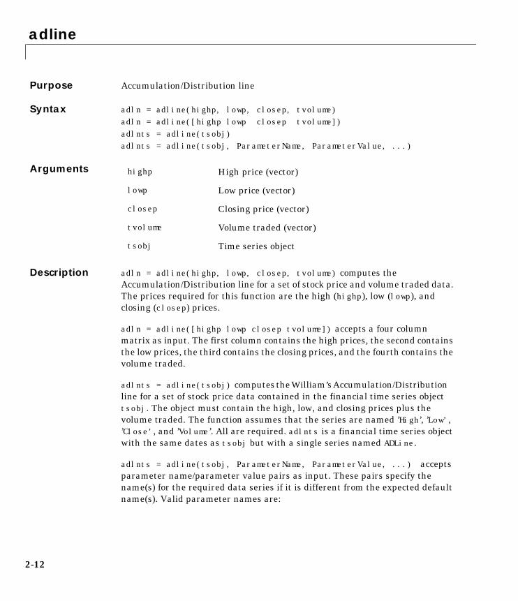
adline
2adlinePurpose Accumulation/Distribution line
Syntax adln = adline(highp, lowp, closep, tvolume)adln = adline([highp lowp closep tvolume])adlnts = adline(tsobj) adlnts = adline(tsobj, ParameterName, ParameterValue, ...)
Arguments
Description adln = adline(highp, lowp, closep, tvolume) computes the Accumulation/Distribution line for a set of stock price and volume traded data. The prices required for this function are the high (highp), low (lowp), and closing (closep) prices.
adln = adline([highp lowp closep tvolume]) accepts a four column matrix as input. The first column contains the high prices, the second contains the low prices, the third contains the closing prices, and the fourth contains the volume traded.
adlnts = adline(tsobj) computes the William’s Accumulation/Distribution line for a set of stock price data contained in the financial time series object tsobj. The object must contain the high, low, and closing prices plus the volume traded. The function assumes that the series are named ’High’, ’Low’, ’Close’, and ’Volume’. All are required. adlnts is a financial time series object with the same dates as tsobj but with a single series named ADLine.
adlnts = adline(tsobj, ParameterName, ParameterValue, ...) accepts parameter name/parameter value pairs as input. These pairs specify the name(s) for the required data series if it is different from the expected default name(s). Valid parameter names are:
highp High price (vector)
lowp Low price (vector)
closep Closing price (vector)
tvolume Volume traded (vector)
tsobj Time series object
2-12

adline
• ’HighName’: high prices series name
• ’LowName’: low prices series name
• ’CloseName’: closing prices series name
• ’VolumeName’: volume traded series name
Parameter values are the strings that represent the valid parameter names.
Example Compute the Accumulation/Distribution line for Disney stock and plot the results.
load disney.matdis_ADLine = adline(dis)plot(dis_ADLine)title(’Accumulation/Distribution Line for Disney’)
See Also adosc, willad, willpctr
2-13

adline
Reference Achelis, Steven B., Technical Analysis From A To Z, Second Printing, McGraw-Hill, 1995, pg. 56 - 58
2-14

adosc
2adoscPurpose Accumulation/Distribution oscillator
Syntax ado = adosc(highp, lowp, openp, closep)ado = adosc([highp lowp openp closep])adots = adosc(tsobj)adots = adosc(tsojb, ParameterName, ParameterValue, ...)
Arguments
Description ado = adosc(highp, lowp, openp, closep) returns a vector, ado, that represents the Accumulation/Distribution (A/D) oscillator. The A/D oscillator is calculated based on the high, low, opening, and closing prices of each period. Each period is treated individually.
ado = adosc([highp lowp openp closep]) accepts a four column matrix as input. The order of the columns must be high, low, opening, and closing prices.
adots = adosc(tsobj) calculates the Accumulation/Distribution (A/D) oscillator, adots, for the set of stock price data contained in the financial time series object tsobj. The object must contain the high, low, opening, and closing prices. The function assumes that the series are named ’High’, ’Low’, ’Open’, and ’Close’. All are required. adots is a financial time series object with similar dates to tsobj and only one series named ’ADOsc’.
adots = adosc(tsobj, ParameterName, ParameterValue, ...) accepts parameter name- parameter value pairs as input. These pairs specify the name(s) for the required data series if it is different from the expected default name(s). Valid parameter names are:
• ’HighName’: high prices series name
• ’LowName’: low prices series name
highp High price (vector)
lowp Low price (vector)
openp Opening price (vector)
closep Closing price (vector)
tsobj Time series object
2-15
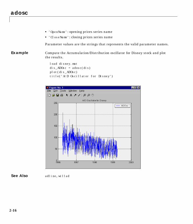
adosc
• ’OpenName’: opening prices series name
• ’CloseName’: closing prices series name
Parameter values are the strings that represents the valid parameter names.
Example Compute the Accumulation/Distribution oscillator for Disney stock and plot the results.
load disney.matdis_ADOsc = adosc(dis)plot(dis_ADOsc)title(’A/D Oscillator for Disney’)
See Also adline, willad
2-16
ascii2fts
2ascii2ftsPurpose Create financial time series object from ASCII data file
Syntax tsobj = ascii2fts(filename, descrow, colheadrow, skiprows)
Arguments
Description tsobj = ascii2fts(filename, descrow, colheadrow, skiprows) creates a financial time series object tsobj from the ASCII file named filename. The general format of the text data file is:
• May contain header text lines
• May contain column header information. The column header information must immediately precede the data series columns.
• Leftmost column must be the date column.
• Dates must be in a valid date string format: ’ddmmmyy’ or ’ddmmmyyyy’’mm/dd/yy’ or ’mm/dd/yyyy’’dd-mmm-yy’ or ’dd-mmm-yyyy’
• Each column must be separated either by spaces or a tab.
Example dis = ascii2fts(’disney.dat’, 1, 3, 2)
See Also fints
filename ASCII data file
descrow (Optional) Row number in the data file that contains the description to be used for the description field of the financial time series object.
colheadrow (Optional) Row that has the column headers/names.
skiprows (Optional) Scalar or vector of consecutive row numbers to be skipped in the data file.
2-17
bollinger
2bollingerPurpose Bollinger band
Syntax [mid, uppr, lowr] = bollinger(data, wsize, wts, nstd)[midfts, upprfts, lowrfts] = bollinger(tsobj, wsize, wts, nstd)
Arguments
Description [mid, uppr, lowr] = bollinger(data, wsize, wts, nstd) calculates the middle, upper, and lower bands that make up the Bollinger bands from the vector data.
mid is the vector that represents the middle band, a simple moving average with default window size of 20. uppr and lowr are vectors that represent the upper and lower bands. These bands are +2 times and -2 times moving standard deviations away from the middle band.
[midfts, upprfts, lowrfts] = bollinger(tsobj, wsize, wts, nstd)calculates the middle, upper, and lower bands that make up the Bollinger bands from a financial time series object tsobj.
midfts is a financial time series object that represents the middle band for all series in tsobj. upprfts and lowrfts are financial time series objects that represent the upper and lower bands of all series, which are +2 times and -2 times moving standard deviations away from the middle band.
data Data vector
wsize (Optional) Window size. Default = 20.
wts (Optional) Weight factor. Determines the type of moving average used. Default = 0 (box). 1= linear.
nstd (Optional) Number of standard deviations for upper and lower bands. Default = 2.
tsobj Financial time series object
2-18

bollinger
Example Compute the Bollinger bands for Disney stock closing prices and plot the results.
load disney.mat[dis_Mid,dis_Uppr,dis_Lowr]= bollinger(dis);dis_CloseBolling = [dis_Mid.CLOSE, dis_Uppr.CLOSE,... dis_Lowr.CLOSE];plot(dis_CloseBolling)title(’Bollinger Bands for Disney Closing Prices’)
See Also tsmovavg
Reference Achelis, Steven B., Technical Analysis From A To Z, Second Printing, McGraw-Hill, 1995, pg. 72 - 74
2-19

boxcox
2boxcoxPurpose Box-Cox transformation
Syntax [transdat, lambda] = boxcox(data)[transdat, lambda] = boxcox(tsobj)transdat = boxcox(data)transdat = boxcox(tsobj)
Arguments
Description boxcox transforms nonnormally distributed data to a set of data that has approximately normal distribution. The Box-Cox transformation is a family of power transformations
The logarithm is the natural logarithm (log base e). The algorithm calls for finding the λ value that maximizes the Log-Likelihood Function (LLF). The search is conducted using fminsearch.
[transdat, lambda] = boxcox(data) transforms the data vector data using the Box-Cox transformation method into transdat. It also calculates the transformation parameter λ.
[transdat, lambda] = boxcox(tsojb) transforms the financial time series object tsobj using the Box-Cox transformation method into transdat.
If the input data is a vector, transdat is also a vector. If the input is a financial time series object, transdat is likewise a financial time series object.
If the input data is a vector, lambda is a scalar. If the input is a financial time series object, lambda is a structure with fields similar to the components of the object, e.g., if the object contains series names Open and Close, lambda has fields lambda.Open and lambda.Close.
data Data vector. Must be positive.
tsobj Financial time series object
data λ( )dataλ 1–
λ------------------------- if λ 0≠
data( ) if λ 0=log
=
2-20
boxcox
transdat = boxcox(lambda, data) and transdat = boxcox(lambda, tsobj) transform the data using a certain specified λ for the Box-Cox transformation. This syntax does not find the optimum λ that maximizes the LLF.
See Also fminsearch
2-21
busdays
2busdaysPurpose Business days in serial date format
Syntax bdates = busdays(sdate, edate, bdmode)bdates = busdays(sdate, edate, bdmode, holvec)
Arguments
Description bdates = busdays(sdate, edate, bdmode) generates a vector of business days, bdates, in serial date format between the start date, sdate, and end date, edate, with frequency, bdmode. The dates are generated based on United States holidays. If you do not supply bdmode, busdays generates a daily vector.
bdates = busdays(sdate, edate, bdmode, holvec) lets you supply a vector of holidays, holvec, used to generate business days. holvec can either be in serial date format or date string format. If you use this syntax, you need to supply the frequency bdmode.
The output, bdates is a column vector of business dates in serial date format.
If you want a weekday vector without the holidays, set holvec to ’’ (empty string) or [] (empty vector).
sdate Start date in string or serial date format
edate End date in string or serial date format
bdmode (Optional) Frequency of business days:DAILY, Daily, daily, D, d, 1 (default)WEEKLY, Weekly, weekly, W, w, 2MONTHLY, Monthly, monthly, M, m, 3QUARTERLY, Quarterly, quarterly, Q, q, 4SEMIANNUAL, Semiannual, semiannual, S, s, 5ANNUAL, Annual, annual, A, a, 6 Strings must be enclosed in single quotes.
holvec (Optional) Holiday dates vector in string or serial date format
2-22
candle
2candlePurpose Candle plot
Syntax candle(tsobj)candle(tsobj, color)candle(tsobj, color, dateform)candle(tsobj, color, dateform, ParameterName, ParameterValue, ...)hdcl = candle(tsobj, color, dateform, ParameterName, ParameterValue,
...)
Arguments
Description candle(tsobj) generates a candle plot of the data in the financial time series object tsobj. tsobj must contain at least four data series representing the high, low, open, and closing prices. These series must have the names ’High’, ’Low’, ’Open’, and ’Close’ (case-insensitive).
candle(tsobj, color) additionally specifies the color of the candle box.
candle(tsobj, color, dateform) additionally specifies the date string format used as the x-axis tick labels. See datestr in the Financial Toolbox User’s Guide for a list of date string formats.
candle(tsobj, color, dateform, ParameterName, ParameterValue, ...) indicates the actual name(s) of the required data series if the data series do not have the default names. ParameterName can be:
• ’HighName’: high prices series name
• ’LowName’: low prices series name
• ’OpenName’: open prices series name
• ’CloseName’: closing prices series name
tsobj Financial time series object
color (Optional) A three-element row vector representing RGB or a color identifier. (See plot in the MATLAB documentation.)
dateform (Optional) Date string format used as the x-axis tick labels. (See datetick in the MATLAB documentation.)
2-23
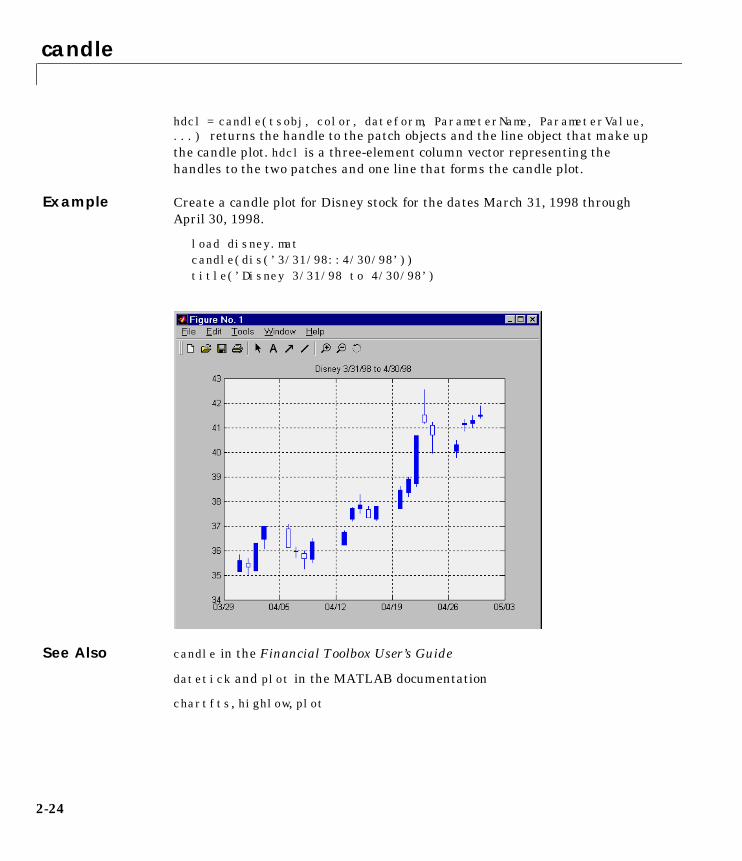
candle
hdcl = candle(tsobj, color, dateform, ParameterName, ParameterValue, ...) returns the handle to the patch objects and the line object that make up the candle plot. hdcl is a three-element column vector representing the handles to the two patches and one line that forms the candle plot.
Example Create a candle plot for Disney stock for the dates March 31, 1998 through April 30, 1998.
load disney.matcandle(dis(’3/31/98::4/30/98’))title(’Disney 3/31/98 to 4/30/98’)
See Also candle in the Financial Toolbox User’s Guide
datetick and plot in the MATLAB documentation
chartfts, highlow, plot
2-24
chaikosc
2chaikoscPurpose Chaikin oscillator
Syntax chosc = chaikosc(highp, lowp, closep, tvolume)chosc = chaikosc([highp lowp closep tvolume])choscts = chaikosc(tsobj)choscts = chaikosc(tsobj, ParameterName, ParameterValue, ... )
Arguments
Description The Chaikin oscillator is calculated by subtracting the 10-period exponential moving average of the Accumulation/Distribution (A/D) line from the three-period exponential moving average of the A/D line.
chosc = chaikosc(highp, lowp, closep, tvolume) calculates the Chaikin oscillator (vector), chosc, for the set of stock price and volume traded data (tvolume). The prices that must be included are the high (highp), low (lowp), and closing (closep) prices.
chosc = chaikosc([highp lowp closep tvolume]) accepts a four-column matrix as input.
choscts = chaikosc(tsobj) calculates the Chaikin Oscillator, choscts, from
the data contained in the financial time series object tsobj. tsobj must at least contain data series with names ’High’, ’Low’, ’Close’, and ’Volume’. These series must represent the high, low, and closing prices, plus the volume traded. choscts is a financial time series object with the same dates as tsobj
but only one series named ’ChaikOsc’.
highp High price (vector)
lowp Low price (vector)
closep Closing price (vector)
tvolume Volume traded (vector)
tsobj Financial time series object
2-25
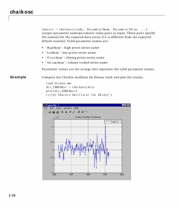
chaikosc
choscts = chaikosc(tsobj, ParameterName, ParameterValue, ...) accepts parameter name/parameter value pairs as input. These pairs specify the name(s) for the required data series if it is different from the expected default name(s). Valid parameter names are:
• ’HighName’: high prices series name
• ’LowName’: low prices series name
• ’CloseName’: closing prices series name
• ’VolumeName’: volume traded series name
Parameter values are the strings that represent the valid parameter names.
Example Compute the Chaikin oscillator for Disney stock and plot the results.
load disney.matdis_CHAIKosc = chaikosc(dis)plot(dis_CHAIKosc)title(’Chaikin Oscillator for Disney’)
2-26
chaikosc
See Also adline
Reference Achelis, Steven B., Technical Analysis From A To Z, Second Printing, McGraw-Hill, 1995, pg. 91 - 94
2-27

chaikvolat
2chaikvolatPurpose Chaikin volatility
Syntax chvol = chaikvolat(highp, lowp)chvol = chaikvolat([highp lowp])chvol = chaikvolat(high, lowp, nperdiff, manper)chvol = chaikvolat([high lowp], nperdiff, manper)chvts = chaikvolat(tsobj)chvts = chaikvolat(tsobj, nperdiff, manper, ParameterName,
ParameterValue, ...)
Arguments
Description chvol = chaikvolat(highp, lowp) calculates the Chaikin volatility from the series of stock prices, highp and lowp. chvol is a vector containing the Chaikin volatility values, calculated on a 10-period exponential moving average and 10-period period difference.
chvol = chaikvolat([highp lowp]) accepts a two-column matrix as the input.
chvol = chaikvolat(high, lowp, nperdiff, manper) manually sets the period difference nperdiff and the length of the exponential moving average manper in periods.
chvol = chaikvolat([high lowp], nperdiff, manper) accepts a two-column matrix as the first input.
chvts = chaikvolat(tsobj) calculates the Chaikin volatility from the financial time series object tsobj. The object must contain at least two series named High and Low, representing the high and low prices per period. chvts is a financial time series object containing the Chaikin volatility values, based on
highp High price (vector)
lowp Low price (vector)
nperdiff Period difference (vector). Default = 10.
manper Length of exponential moving average in periods (vector). Default = 10.
tsobj Financial time series object
2-28
chaikvolat
a 10-period exponential moving average and 10-period period difference. chvts has the same dates as tsobj and a series called ChaikVol.
chvts = chaikvolat(tsobj, nperdiff, manper, ParameterName, ParameterValue, ...) accepts parameter name/parameter value pairs as input. These pairs specify the name(s) for the required data series if it is different from the expected default name(s). Valid parameter names are:
• ’HighName’: high prices series name
• ’LowName’: low prices series name
Parameter values are the strings that represent the valid parameter names.
nperdiff, the period difference, and manper, the length of the exponential moving average in periods, can also be set with this form of chaikvolat.
Example Compute the Chaikin volatility for Disney stock and plot the results.
load disney.matdis_CHAIKvol = chaikvolat(dis)plot(dis_CHAIKvol)title(’Chaikin Volatility for Disney’)
2-29

chaikvolat
See Also chaikosc
Reference Achelis, Steven B., Technical Analysis From A To Z, Second Printing, McGraw-Hill, 1995, pg. 304 - 305
2-30
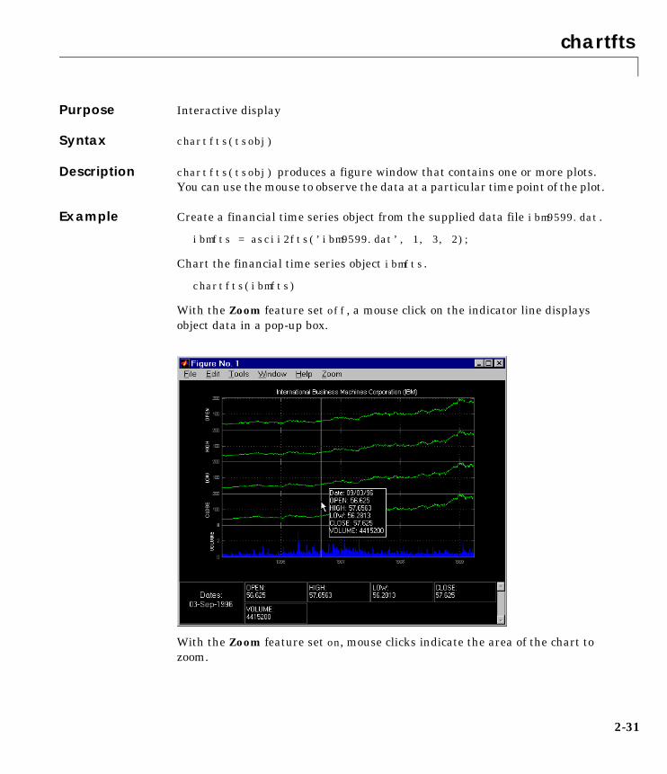
chartfts
2chartftsPurpose Interactive display
Syntax chartfts(tsobj)
Description chartfts(tsobj) produces a figure window that contains one or more plots. You can use the mouse to observe the data at a particular time point of the plot.
Example Create a financial time series object from the supplied data file ibm9599.dat.
ibmfts = ascii2fts(’ibm9599.dat’, 1, 3, 2);
Chart the financial time series object ibmfts.
chartfts(ibmfts)
With the Zoom feature set off, a mouse click on the indicator line displays object data in a pop-up box.
With the Zoom feature set on, mouse clicks indicate the area of the chart to zoom.
2-31

chartfts
See the instructions provided by Zoom Help for details on performing the zoom.
See Also candle, highlow, plot
2-32
chfield
2chfieldPurpose Change data series name
Syntax newfts = chfield(oldfts, oldname, newname)
Arguments
Description newfts = chfield(oldfts, oldname, newname) changes the name of the financial time series object component from oldname to newname.
Set newfts = oldfts to change the name of an existing component without changing the name of the financial time series object.
To change the names of several components at once, specify the series of old and new component names in corresponding column cell arrays.
You cannot change the names of the object components ’desc’, ’freq’, and ’dates’.
See Also fieldnames, isfield, rmfield
oldfts Name of an existing financial time series object
oldname Name of the existing component in oldfts. A MATLAB string or column cell array.
newname New name for the component in oldfts. A MATLAB string or column cell array.
2-33
convertto
2converttoPurpose Convert to specified frequency
Syntax newfts = convertto(oldfts, newfreq)
Arguments
Description convertto converts a financial time series of any frequency to one of a specified frequency. It makes some assumptions regarding the dates in the resulting time series.
newfts = convertto(oldfts, newfreq) converts the object oldfts to the new time series object newfts with the frequency newfreq.
See Also toannual, todaily, tomonthly, toquarterly, tosemi, toweekly
newfreq 1, DAILY, Daily, daily, D, d 2, WEEKLY, Weekly, weekly, W, w 3, MONTHLY, Monthly, monthly, M, m 4, QUARTERLY, Quarterly, quarterly, Q, q 5, SEMIANNUAL, Semiannual, semiannual, S, s 6, ANNUAL, Annual, annual, A, a
2-34
demts2fts
2demts2ftsPurpose Convert demo time series to financial time series object
Syntax tsobj = demts2fts(demts)
Description tsobj = demts2fts(demts) converts a demonstration time series object into a financial time series object. A demonstration time series object is a time series object created using the time series capabilities of the Financial Toolbox. tsobj has a single data series named series1.
See Also fints
2-35
diff
2diffPurpose Differencing
Syntax newfts = diff(oldfts)
Description diff computes the differences of the data series in a financial time series object. It returns another time series object containing the difference.
newfts = diff(oldfts) computes the difference of all the data in the data series of the object oldfts and returns the result in the object newfts. newfts is a financial time series object containing the same data series (names) as the input oldfts.
See Also diff in the MATLAB documentation
2-36
display
2displayPurpose Display financial time series object
Syntax display(tsobj)
Description display displays a financial time series object in the command window. Numeric values inherit the format specified in MATLAB.
Note Although the contents of the object display as cells of a cell array, the object itself is not a cell array.
See Also format in the MATLAB documentation
2-37

end
2endPurpose Last date entry
Syntax end
Description end returns the index to the last date entry in a financial time series object.
Example Consider a financial time series object called fts:
fts =
desc: DJI30MAR94.datfreq: Daily (1)
’dates: (20)’ ’Open: (20)’ ’04-Mar-1994’ [ 3830.9]’07-Mar-1994’ [ 3851.7]’08-Mar-1994’ [ 3858.5]’09-Mar-1994’ [ 3854]’10-Mar-1994’ [ 3852.6]’11-Mar-1994’ [ 3832.6]’14-Mar-1994’ [ 3870.3]’16-Mar-1994’ [ 3851]’17-Mar-1994’ [ 3853.6]’18-Mar-1994’ [ 3865.4]’21-Mar-1994’ [ 3878.4]’22-Mar-1994’ [ 3865.7]’23-Mar-1994’ [ 3868.9]’24-Mar-1994’ [ 3849.9]’25-Mar-1994’ [ 3827.1]’28-Mar-1994’ [ 3776.5]’29-Mar-1994’ [ 3757.2]’30-Mar-1994’ [ 3688.4]’31-Mar-1994’ [ 3639.7]
2-38

end
The command fts(15:end)returns
ans =
desc: DJI30MAR94.datfreq: Daily (1)
’dates: (6)’ ’Open: (6)’ ’24-Mar-1994’ [ 3849.9]’25-Mar-1994’ [ 3827.1]’28-Mar-1994’ [ 3776.5]’29-Mar-1994’ [ 3757.2]’30-Mar-1994’ [ 3688.4]’31-Mar-1994’ [ 3639.7]
See Also subsasgn, subsref
end in the MATLAB documentation
2-39
exp
2expPurpose Exponential values
Syntax newfts = exp(tsobj)
Description newfts = exp(tsobj) calculates the natural exponential (base e) of all the data in the data series of the financial time series object tsobj and returns the result in the object newfts.
See Also log, log10
2-40
extfield
2extfieldPurpose Extract data series
Syntax ftse = extfield(tsobj, fieldnames)
Arguments
Description ftse = extfield(tsobj, fieldnames) extracts from tsobj the dates and data series specified by fieldnames into a new financial time series object ftse. ftse has all the dates in tsobj but contains a smaller number of data series.
Example extfield is identical to referencing a field in the object. For example
ftse = extfield(fts, ’Close’)
is the same as
ftse = fts.Close
This function is the complement of the function rmfield.
See Also rmfield
tsobj Financial time series object
fieldnames Data series to be extracted. A cell array if a list of data series names (field names) is supplied. A string if only one is wanted.
2-41

fieldnames
2fieldnamesPurpose Get names of fields
Syntax fnames = fieldnames(tsobj)fnames = fieldnames(tsobj, srsnameonly)
Arguments
Description fieldnames gets field names in a financial time series object.
fnames = fieldnames(tsobj) returns the field names associated with the financial time series object tsobj as a cell array of strings, including the common minimum fields: desc, freq, and dates.
fnames = fieldnames(tsobj, srsnameonly) returns fieldnames depending upon the setting of srsnameonly. If srsnameonly is 0, all fieldnames are returned, including the common minimum fields: desc, freq, and dates. If srsnameonly is set to 1, only the data series name(s) are returned in fnames.
See Also chfield, getfield, isfield, rmfield, setfield
tsobj Financial time series object
srsnameonly Field names returned:0 = all field names (default).1 = data series names only.
2-42

fillts
2filltsPurpose Fill missing values in time series
Syntax newfts = fillts(oldfts, fill_method)newfts = fillts(oldfts, fill_method, newdates)newfts = fillts(oldfts, fill_method, newdates, sortmode)
Arguments
Description newfts = fillts(oldfts, fill_method) replaces missing values (represented by NaN) in the financial time series object oldfts with real values, using the interpolation process indicated by fill_method.
newfts = fillts(oldfts, fill_method, newdates) replaces all the missing values on the specified dates newdates in the financial time series oldfts with new values through an interpolation process using fill_method. fill_method can be ’linear’, ’cubic’, ’spline’, or ’nearest’. If any of the dates in newdates exist in oldfts, the existing one has precedence. If newdates contains dates outside the boundary of oldfts, the values for those dates will be NaN’s.
newfts = fillts(oldts, fillmethod, newdates, sortmode) additionally denotes whether you want the order of the dates in the output object to stay the same as in the input object or to be sorted chronologically.
sortmode = 0 (unsorted) appends any new dates to the end. The interpolation process that calculates the values for the new dates works on a sorted object. Upon completion, the existing dates are reordered as they were originally, and the new dates are appended to the end.
sortmode = 1 sorts the output. After interpolation, no reordering of date sequence occurs.
See Also interp1 in the MATLAB documentation
fill_method (Optional) Values may be ’linear ’(default), ’cubic’, ’spline’, or ’nearest’.
newdates (Optional) Column vector of serial dates, a date string, or a column cell array of date strings
sortmode (Optional) Default = 0 (unsorted). 1 = sorted.
2-43
filter
2filterPurpose Linear filtering
Syntax newfts = filter(B, A, oldfts)
Description filter filters a whole financial time series object with certain filter specifications. The filter is specified in a transfer function expression.
newfts = filter(B, A, oldfts) filters the data in the financial time series object oldfts with the filter described by vectors A and B to create the new financial time series object newfts. The filter is a “Direct Form II Transposed” implementation of the standard difference equation. newfts is a financial time series object containing the same data series (names) as the input oldfts.
See Also filter, filter2 in the MATLAB documentation
2-44
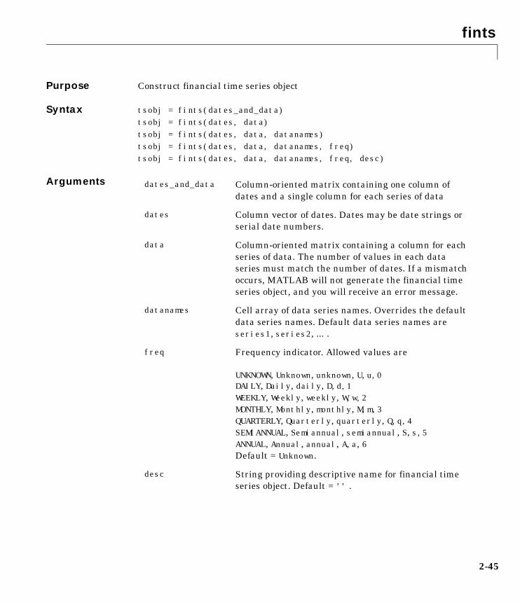
fints
2fintsPurpose Construct financial time series object
Syntax tsobj = fints(dates_and_data)tsobj = fints(dates, data)tsobj = fints(dates, data, datanames)tsobj = fints(dates, data, datanames, freq)tsobj = fints(dates, data, datanames, freq, desc)
Arguments dates_and_data Column-oriented matrix containing one column of dates and a single column for each series of data
dates Column vector of dates. Dates may be date strings or serial date numbers.
data Column-oriented matrix containing a column for each series of data. The number of values in each data series must match the number of dates. If a mismatch occurs, MATLAB will not generate the financial time series object, and you will receive an error message.
datanames Cell array of data series names. Overrides the default data series names. Default data series names are series1, series2, ... .
freq Frequency indicator. Allowed values are
UNKNOWN, Unknown, unknown, U, u,0DAILY, Daily, daily, D, d,1 WEEKLY, Weekly, weekly, W, w,2 MONTHLY, Monthly, monthly, M, m, 3 QUARTERLY, Quarterly, quarterly, Q, q,4 SEMIANNUAL, Semiannual, semiannual, S, s,5 ANNUAL, Annual, annual, A, a, 6Default = Unknown.
desc String providing descriptive name for financial time series object. Default = ’’ .
2-45
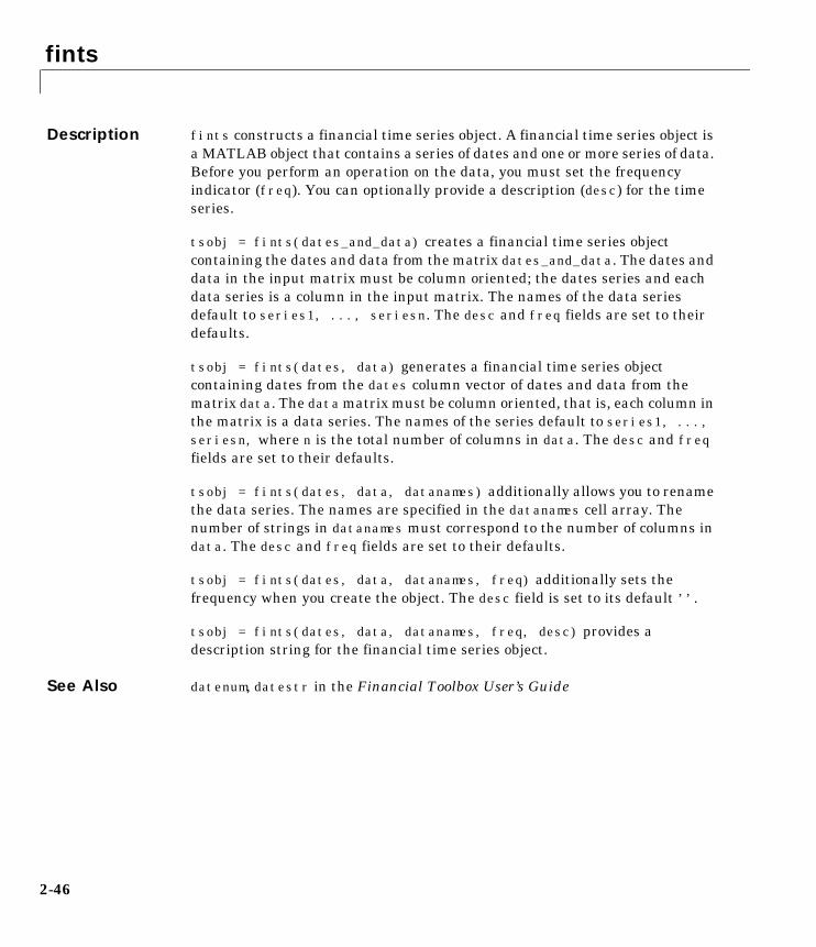
fints
Description fints constructs a financial time series object. A financial time series object is a MATLAB object that contains a series of dates and one or more series of data. Before you perform an operation on the data, you must set the frequency indicator (freq). You can optionally provide a description (desc) for the time series.
tsobj = fints(dates_and_data) creates a financial time series object containing the dates and data from the matrix dates_and_data. The dates and data in the input matrix must be column oriented; the dates series and each data series is a column in the input matrix. The names of the data series default to series1, ..., seriesn. The desc and freq fields are set to their defaults.
tsobj = fints(dates, data) generates a financial time series object containing dates from the dates column vector of dates and data from the matrix data. The data matrix must be column oriented, that is, each column in the matrix is a data series. The names of the series default to series1, ..., seriesn, where n is the total number of columns in data. The desc and freq fields are set to their defaults.
tsobj = fints(dates, data, datanames) additionally allows you to rename the data series. The names are specified in the datanames cell array. The number of strings in datanames must correspond to the number of columns in data. The desc and freq fields are set to their defaults.
tsobj = fints(dates, data, datanames, freq) additionally sets the frequency when you create the object. The desc field is set to its default ’’.
tsobj = fints(dates, data, datanames, freq, desc) provides a description string for the financial time series object.
See Also datenum, datestr in the Financial Toolbox User’s Guide
2-46

fpctkd
2fpctkdPurpose Fast stochastics
Syntax [pctk, pctd] = fpctkd(highp, lowp, closep)[pctk, pctd] = fpctkd([highp lowp closep])[pctk, pctd] = fpctkd(highp, lowp, closep, kperiods, dperiods,
dmamethod)[pctk, pctd]= fpctkd([highp lowp closep], kperiods, dperiods,
dmamethod)pkts = fpctkd(tsobj, kperiods, dperiods, dmamethod)pkts = fpctkd(tsobj, kperiods, dperiods, dmamethod, ParameterName,
ParameterValue, ...)
Arguments
Description fpctkd calculates the stochastic oscillator.
[pctk, pctd] = fpctkd(highp, lowp, closep) calculates the Fast PercentK (F%K) and Fast PercentD (F%D) from the stock price data, highp (high prices), lowp (low prices), and closep (closing prices).
[pctk, pctd] = fpctkd([highp lowp closep]) accepts a three-column matrix of high (highp), low (lowp), and closing prices (closep), in that order.
[pctk, pctd] = fpctkd(highp, lowp, closep, kperiods, dperiods, dmamethod) calculates Fast PercentK (F%K) and Fast PercentD (F%D) from the stock price data, highp (high prices), lowp (low prices), and closep (closing prices). kperiods sets the %K period. dperiods sets the %D period.
highp High price (vector)
lowp Low price (vector)
closep Closing price (vector)
kperiods (Optional) %K periods. Default = 10.
dperiods (Optional) %D periods. Default = 3.
damethod (Optional) %D moving average method. Default = ’e’ (exponential).
tsobj Financial time series object
2-47

fpctkd
damethod specifies the %D moving average method. Valid moving average methods for %D are Exponential (’e’) and Triangular (’t’). See tsmovavg for explanations of these methods.
[pctk, pctd]= fpctkd([highp lowp closep], kperiods, dperiods, dmamethod) accepts a three-column matrix of high (highp), low (lowp), and closing prices (closep), in that order.
pkts = fpctkd(tsobj, kperiods, dperiods, dmamethod) calculates the Fast PercentK (F%K) and Fast PercentD (F%D) from the stock price data in the financial time series object tsobj. tsobj must minimally contain the series High (high prices), Low (low prices), and Close (closing prices). pkts is a financial time series object with similar dates to tsobj and two data series named PercentK and PercentD.
pkts = fpctkd(tsobj, kperiods, dperiods, dmamethod, ParameterName, ParameterValue, ...) accepts parameter name/parameter value pairs as input. These pairs specify the name(s) for the required data series if it is different from the expected default name(s). Valid parameter names are:
• ’HighName’: high prices series name
• ’LowName’: low prices series name
• ’CloseName’: closing prices series name
Parameter values are the strings that represent the valid parameter names.
2-48

fpctkd
Example Compute the stochastic oscillator for Disney stock and plot the results.
load disney.matdis_FastStoc = fpctkd(dis)plot(dis_FastStoc)title(’Stochastic Oscillator for Disney’)
See Also spctkd, stochosc, tsmovavg
Reference Achelis, Steven B., Technical Analysis From A To Z, Second Printing, McGraw-Hill, 1995, pg. 268 - 271
2-49
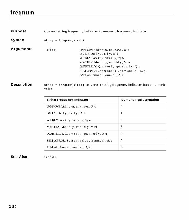
freqnum
2freqnumPurpose Convert string frequency indicator to numeric frequency indicator
Syntax nfreq = freqnum(sfreq)
Arguments
Description nfreq = freqnum(sfreq) converts a string frequency indicator into a numeric value.
See Also freqstr
sfreq UNKNOWN, Unknown, unknown, U, uDAILY, Daily, daily, D, d WEEKLY, Weekly, weekly, W, w MONTHLY, Monthly, monthly, M, m QUARTERLY, Quarterly, quarterly, Q, q SEMIANNUAL, Semiannual, semiannual, S, s ANNUAL, Annual, annual, A, a
String Frequency Indicator Numeric Representation
UNKNOWN, Unknown, unknown, U, u 0
DAILY, Daily, daily, D, d 1
WEEKLY, Weekly, weekly, W, w 2
MONTHLY, Monthly, monthly, M, m 3
QUARTERLY, Quarterly, quarterly, Q, q 4
SEMIANNUAL, Semiannual, semiannual, S, s 5
ANNUAL, Annual, annual, A, a 6
2-50

freqstr
2freqstrPurpose Convert numeric frequency indicator to string representation
Syntax sfreq = freqstr(nfreq)
Arguments
Description sfreq = freqstr(nfreq) converts a numeric frequency indicator into a string representation.
See Also freqnum
nfreq 0123456
Numeric Frequency Indicator String Representation
0 Unknown
1 Daily
2 Weekly
3 Monthly
4 Quarterly
5 Semiannual
6 Annual
2-51
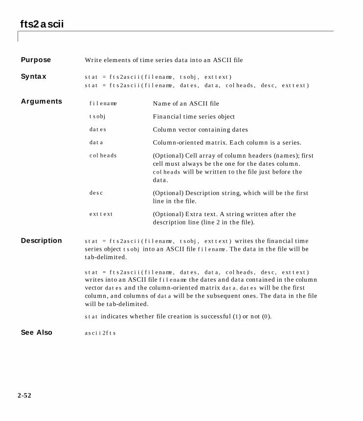
fts2ascii
2fts2asciiPurpose Write elements of time series data into an ASCII file
Syntax stat = fts2ascii(filename, tsobj, exttext)stat = fts2ascii(filename, dates, data, colheads, desc, exttext)
Arguments
Description stat = fts2ascii(filename, tsobj, exttext) writes the financial time series object tsobj into an ASCII file filename. The data in the file will be tab-delimited.
stat = fts2ascii(filename, dates, data, colheads, desc, exttext) writes into an ASCII file filename the dates and data contained in the column vector dates and the column-oriented matrix data. dates will be the first column, and columns of data will be the subsequent ones. The data in the file will be tab-delimited.
stat indicates whether file creation is successful (1) or not (0).
See Also ascii2fts
filename Name of an ASCII file
tsobj Financial time series object
dates Column vector containing dates
data Column-oriented matrix. Each column is a series.
colheads (Optional) Cell array of column headers (names); first cell must always be the one for the dates column. colheads will be written to the file just before the data.
desc (Optional) Description string, which will be the first line in the file.
exttext (Optional) Extra text. A string written after the description line (line 2 in the file).
2-52
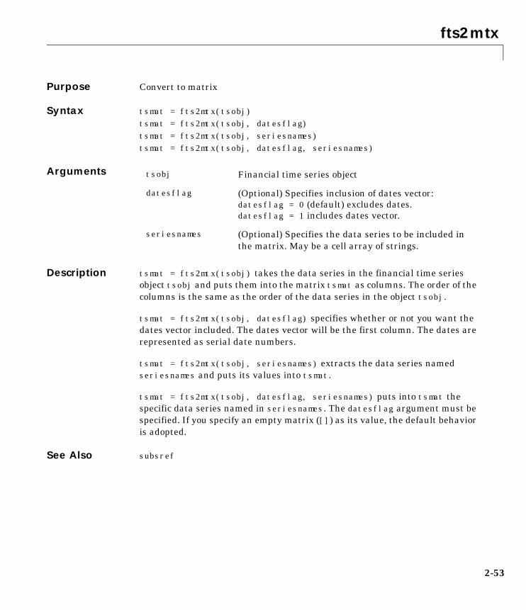
fts2mtx
2fts2mtxPurpose Convert to matrix
Syntax tsmat = fts2mtx(tsobj)tsmat = fts2mtx(tsobj, datesflag)tsmat = fts2mtx(tsobj, seriesnames) tsmat = fts2mtx(tsobj, datesflag, seriesnames)
Arguments
Description tsmat = fts2mtx(tsobj) takes the data series in the financial time series object tsobj and puts them into the matrix tsmat as columns. The order of the columns is the same as the order of the data series in the object tsobj.
tsmat = fts2mtx(tsobj, datesflag) specifies whether or not you want the dates vector included. The dates vector will be the first column. The dates are represented as serial date numbers.
tsmat = fts2mtx(tsobj, seriesnames) extracts the data series named seriesnames and puts its values into tsmat.
tsmat = fts2mtx(tsobj, datesflag, seriesnames) puts into tsmat the specific data series named in seriesnames. The datesflag argument must be specified. If you specify an empty matrix ([]) as its value, the default behavior is adopted.
See Also subsref
tsobj Financial time series object
datesflag (Optional) Specifies inclusion of dates vector:datesflag = 0 (default) excludes dates.datesflag = 1 includes dates vector.
seriesnames (Optional) Specifies the data series to be included in the matrix. May be a cell array of strings.
2-53
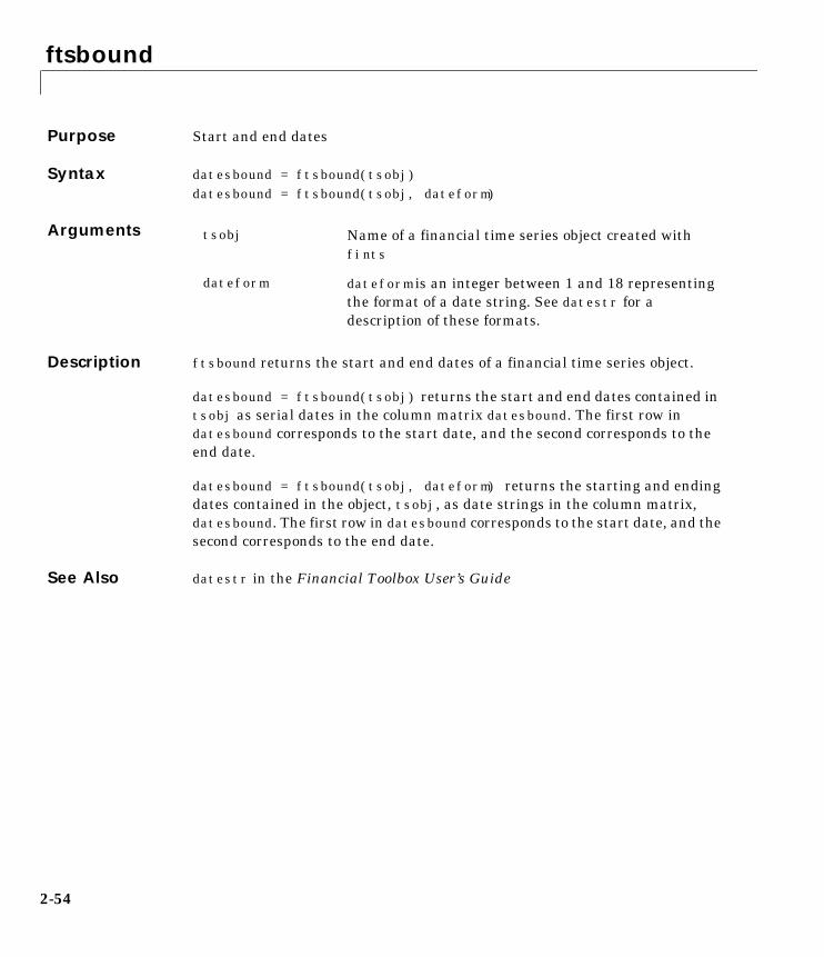
ftsbound
2ftsboundPurpose Start and end dates
Syntax datesbound = ftsbound(tsobj)datesbound = ftsbound(tsobj, dateform)
Arguments
Description ftsbound returns the start and end dates of a financial time series object.
datesbound = ftsbound(tsobj) returns the start and end dates contained in tsobj as serial dates in the column matrix datesbound. The first row in datesbound corresponds to the start date, and the second corresponds to the end date.
datesbound = ftsbound(tsobj, dateform) returns the starting and ending dates contained in the object, tsobj, as date strings in the column matrix, datesbound. The first row in datesbound corresponds to the start date, and the second corresponds to the end date.
See Also datestr in the Financial Toolbox User’s Guide
tsobj Name of a financial time series object created with fints
dateform dateform is an integer between 1 and 18 representing the format of a date string. See datestr for a description of these formats.
2-54
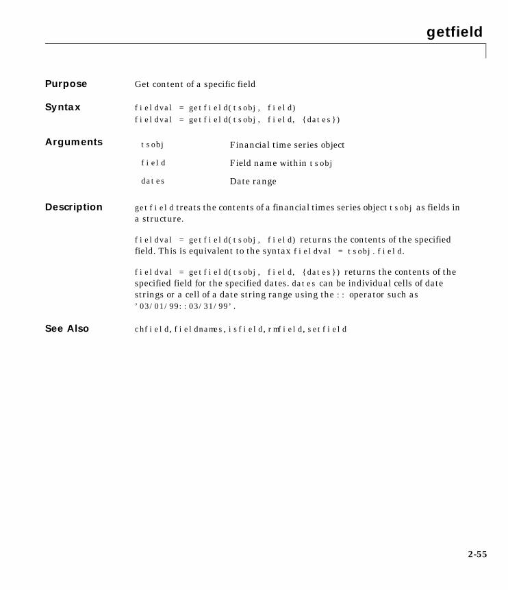
getfield
2getfieldPurpose Get content of a specific field
Syntax fieldval = getfield(tsobj, field)fieldval = getfield(tsobj, field, {dates})
Arguments
Description getfield treats the contents of a financial times series object tsobj as fields in a structure.
fieldval = getfield(tsobj, field) returns the contents of the specified field. This is equivalent to the syntax fieldval = tsobj.field.
fieldval = getfield(tsobj, field, {dates}) returns the contents of the specified field for the specified dates. dates can be individual cells of date strings or a cell of a date string range using the :: operator such as ’03/01/99::03/31/99’.
See Also chfield, fieldnames, isfield, rmfield, setfield
tsobj Financial time series object
field Field name within tsobj
dates Date range
2-55
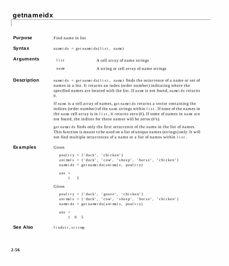
getnameidx
2getnameidxPurpose Find name in list
Syntax nameidx = getnameidx(list, name)
Arguments
Description nameidx = getnameidx(list, name) finds the occurrence of a name or set of names in a list. It returns an index (order number) indicating where the specified names are located with the list. If name is not found, nameidx returns 0.
If name is a cell array of names, getnameidx returns a vector containing the indices (order number) of the name strings within list. If none of the names in the name cell array is in list, it returns zero (0). If some of names in name are not found, the indices for these names will be zeros (0’s).
getnameidx finds only the first occurrence of the name in the list of names. This function is meant to be used on a list of unique names (strings) only. It will not find multiple occurrences of a name or a list of names within list.
Examples Given
poultry = {’duck’, ’chicken’}animals = {’duck’, ’cow’, ’sheep’, ’horse’, ’chicken’}nameidx = getnameidx(animals, poultry)
ans =1 5
Given
poultry = {’duck’, ’goose’, ’chicken’}animals = {’duck’, ’cow’, ’sheep’, ’horse’, ’chicken’}nameidx = getnameidx(animals, poultry)
ans =1 0 5
See Also findstr, strcmp
list A cell array of name strings
name A string or cell array of name strings
2-56

hhigh
2hhighPurpose Highest high
Syntax hhv = hhigh(data)hhv = hhigh(data, nperiods, dim)hhvts = hhigh(tsobj, nperiods)hhvts = hhigh(tsobj, nperiods, ParameterName, ParameterValue)
Arguments
Description hhv = hhigh(data) generates a vector of highest high values the past 14 periods from the matrix data.
hhv = hhigh(data, nperiods, dim) generates a vector of highest high values the past nperiods periods. dim indicates the direction in which the highest high is to be searched. If you input [] for nperiods, the default is 14.
hhvts = hhigh(tsobj, nperiods) generates a vector of highest high values from tsobj, a financial time series object. tsobj must include at least the series High. The output hhvts is a financial time series object with the same dates as tsobj and data series named HighestHigh. If nperiods is specified, hhigh generates a financial time series object of highest high values for the past nperiods periods.
hhvts = hhigh(tsobj, nperiods, ParameterName, ParameterValue)specifies the name for the required data series when it is different from the default name. The valid parameter name is:
• ’HighName’: high prices series name
The parameter value is a string that represents the valid parameter name.
data Data series matrix
nperiods (Optional) Number of periods. Default = 14.
dim (Optional) Dimension
tsobj Financial time series object
2-57

hhigh
Example Compute the highest high prices for Disney stock and plot the results.
load disney.matdis_HHigh = hhigh(dis)plot(dis_HHigh)title(’Highest High for Disney’)
See Also llow
2-58

highlow
2highlowPurpose High-Low plot
Syntax highlow(tsobj)highlow(tsobj, color)highlow(tsobj, color, dateform)highlow(tsobj, color, dateform, ParameterName, ParameterValue, ...)hhll = highlow(tsobj, color, dateform, ParameterName,
ParameterValue, ...)
Arguments
Description highlow(tsobj) generates a High-Low plot of the data in the financial time series object tsobj. tsobj must contain at least four data series representing the high, low, open, and closing prices. These series must have the names ’High’, ’Low’, ’Open’, and ’Close’ (case-insensitive).
highlow(tsobj, color) additionally specifies the color of the plot.
highlow(tsobj, color, dateform) additionally specifies the date string format used as the x-axis tick labels. See datestr in the Financial Toolbox User’s Guide for a list of date string formats.
highlow(tsobj, color, dateform, ParameterName, ParameterValue,...) indicates the actual name(s) of the required data series if the data series do not have the default names. ParameterName can be:
• ’HighName’: high prices series name
• ’LowName’: low prices series name
• ’OpenName’: open prices series name
• ’CloseName’: closing prices series name
tsobj Financial time series object
color (Optional) A three-element row vector representing RGB or a color identifier. (See plot in the MATLAB documentation.)
dateform (Optional) Date string format used as the x-axis tick labels. (See datetick in the MATLAB documentation.)
2-59
highlow
hhll = candle(tsobj, color, dateform, ParameterName, ParameterValue, ...) returns the handle to the line object that makes up the High-Low plot.
See Also highlow in the Financial Toolbox User’s Guide
datetick and plot in the MATLAB documentation
candle
2-60
hist
2histPurpose Histogram
Syntax hist(tsobj, numbins)ftshist = hist(tsobj, numbins)[ftshist, binpos] = hist(tsobj, numbins)
Arguments
Description hist(tsobj, numbins) calculates and displays the histogram of the data series contained in the financial time series object tsobj.
ftshist = hist(tsobj, numbins) calculates, but does not display, the histogram of the data series contained in the financial time series object tsobj. ftshist is a structure with field names similar to the data series names of tsobj.
[ftshist, binpos] = hist(tsobj, numbins) additionally returns the bin positions binpos. The positions are the centers of each bin. binpos is a column vector.
Example Create a histogram of Disney open, high, low, and close prices.
load disney.matdis = rmfield(dis,’VOLUME’) % remove VOLUME fieldhist(dis)title(’Disney Histogram’)
tsobj Financial time series object
numbins (Optional) Number of histogram bins. Default = 10.
2-61

hist
See Also hist in the MATLAB documentation
mean, std
2-62

horzcat
2horzcat Purpose Concatenate financial time series objects horizontally
Syntax newfts = horzcat(tsobj1, tsobj2, ...)
Description horzcat implements horizontal concatenation of financial time series objects. horzcat essentially merges the data columns of the financial time series objects. All time series objects must have the exact same dates.
When multiple instances of a data series name occur, concatenation adds a suffix to the current names of the data series. The suffix has the format _objectname<n>, where n is a number indicating the position of the time series, from left to right, in the concatenation command. The n part of the suffix appears only when there is more than one instance of a particular data series name.
The description fields will be concatenated as well. They will be separated by //.
Example Construct three financial time series each containing a data series named DataSeries.
firstfts = fints((today:today+4)’, (1:5)’,’DataSeries’,’d’);secondfts = fints((today:today+4)’, (11:15)’,’DataSeries’,’d’);thirdfts = fints((today:today+4)’, (21:25)’,’DataSeries’,’d’);
Concatenate the time series horizontally into a new financial time series newfts.
newfts = [firstfts secondfts thirdfts secondfts];
The resulting object newfts has data series names: DataSeries_firstfts, DataSeries_secondfts2, DataSeries_thirdfts, and DataSeries_secondfts4. Verify this with the command
fieldnames(newfts)
ans =
’desc’’freq’’dates’’DataSeries_firstfts’
2-63

horzcat
’DataSeries_secondfts2’’DataSeries_thirdfts’’DataSeries_secondfts4’
Use chfield to change the data series names.
Note If all input objects have the same frequency, the new object has that frequency as well. However, if one of the objects concatenated has a different frequency than the others, the frequency indicator of the resulting object is set to Unknown (0).
See Also vertcat
2-64
iscompatible
2iscompatiblePurpose Structural equality
Syntax iscomp = iscompatible(tsobj_1, tsobj_2)
Description iscomp = iscompatible(tsobj_1, tsobj_2) returns 1 if both financial time series objects tsobj_1 and tsobj_2 have the same dates and data series names. It returns 0 if any component is different.
iscomp = 1 indicates that the two objects contain the same number of data points as well as equal number of data series. However, the values contained in the data series can be different.
Note Data series names are case-sensitive.
See Also isequal
2-65

isequal
2isequalPurpose Multiple object equality
Syntax iseq = isequal(tsobj_1, tsobj_2, ...)
Arguments
Description iseq = isequal(tsobj_1, tsobj_2, ...) returns 1 if all listed financial time series objects have the same dates, data series names, and values contained in the data series. It returns 0 if any of those components is different.
Note Data series names are case-sensitive.
iseq = 1 implies that each object contains the same number of dates and the same data. Only the descriptions may differ.
See Also iscompatible
tsobj_1 ... A list of financial time series objects
2-66

isfield
2isfieldPurpose Check if string is a field name
Syntax F = isfield(tsobj, name)
Description F = isfield(tsobj, name) returns true (1) if name is the name of a data series in tsobj. Otherwise, isfield returns false (0).
See Also fieldnames, getfield, setfield
2-67

lagts
2lagtsPurpose Lag time series object
Syntax newfts = lagts(oldfts)newfts = lagts(oldfts, lagperiod)newfts = lagts(oldfts, lagperiod, padmode)
Arguments
Description lagts delays a financial time series object values by a specified time step.
newfts = lagts(oldfts) delays the data series in oldfts by one time series date entry and returns the result in the object newfts. The end will be padded with zeros, by default.
newfts = lagts(oldfts, lagperiod) shifts time series values to the right on an increasing time scale. lagts delays the data series to happen at a later time. lagperiod is the number of lag periods expressed in the frequency of the time series object oldfts. For example, if oldfts is a daily time series, lagperiod is specified in days. lagts pads the data with zeros (default).
newfts = lagts(oldfts, lagperiod, padmode) lets you pad the data with a value, NaN, or Inf rather than zeros by setting padmode to the desired value.
See Also leadts
oldfts Financial time series object
lagperiod Number of lag periods expressed in the frequency of the time series object
padmode Data padding value
2-68
leadts
2leadtsPurpose Lead time series object
Syntax newfts = leadts(oldfts)newfts = leadts(oldfts, leadperiod)newfts = leadts(oldfts, leadperiod, padmode)
Arguments
Description leadts advances a financial time series object values by a specified time step.
newfts = leadts(oldfts) advances the data series in oldfts by one time series date entry and returns the result in the object newfts. The end will be padded with zeros, by default.
newfts = leadts(oldfts, leadperiod) shifts time series values to the left on an increasing time scale. leadts advances the data series to happen at an earlier time. leadperiod is the number of lead periods expressed in the frequency of the time series object oldfts. For example, if oldfts is a daily time series, leadperiod is specified in days. leadts pads the data with zeros (default).
newfts = leadts(oldfts, leadperiod, padmode) lets you pad the data with a value, NaN, or Inf rather than zeros by setting padmode to the desired value.
See Also lagts
oldfts Financial time series object
leadperiod Number of lead periods expressed in the frequency of the time series object
padmode Data padding value
2-69

length
2lengthPurpose Get number of dates (rows)
Syntax lenfts = length(tsobj)
Description lenfts = length(tsobj) returns the number of dates (rows) in the financial time series object tsobj. This is the same as issuing lenfts = size(tsobj, 1).
See Also length in the MATLAB documentation
size
2-70
llow
2llowPurpose Lowest low
Syntax llv = llow(data)llv = llow(data, nperiods, dim)llvts = llow(tsobj, nperiods)llvts = llow(tsobj, nperiods, ParameterName, ParameterValue)
Arguments
Description llv = llow(data) generates a vector of lowest low values the past 14 periods from the matrix data.
llv = llow(data, nperiods, dim) generates a vector of lowest low values the past nperiods periods. dim indicates the direction in which the lowest low is to be searched. If you input [] for nperiods, the default is 14.
llvts = llow(tsobj, nperiods) generates a vector of lowest low values from tsobj, a financial time series object. tsobj must include at least the series Low. The output llvts is a financial time series object with the same dates as tsobj and data series named LowestLow. If nperiods is specified, llow generates a financial time series object of lowest low values for the past nperiods periods.
llvts = llow(tsobj, nperiods, ParameterName, ParameterValue)specifies the name for the required data series when it is different from the default name. The valid parameter name is:
• LowName: low prices series name
The parameter value is a string that represents the valid parameter name.
data Data series matrix
nperiods (Optional) Number of periods. Default = 14.
dim Dimension
tsobj Financial time series object
2-71
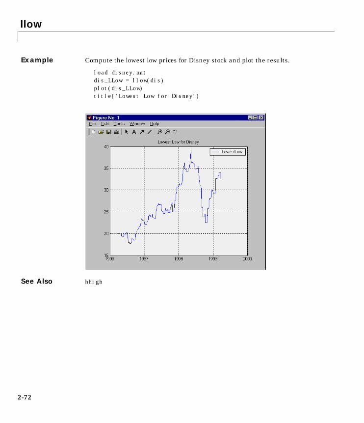
llow
Example Compute the lowest low prices for Disney stock and plot the results.
load disney.matdis_LLow = llow(dis)plot(dis_LLow)title(’Lowest Low for Disney’)
See Also hhigh
2-72
log
2logPurpose Natural logarithm
Syntax newfts = log(tsobj)
Description newfts = log(tsobj) calculates the natural logarithm (log base e) of the data series in a financial time series object tsobj. It returns another time series object containing the natural logarithms.
See Also exp, log10
2-73
log10
2log10Purpose Common logarithm
Syntax newfts = log10(tsobj)
Description newfts = log10(tsobj) calculates the common logarithm (base 10) of all the data in the data series of the financial time series object tsobj and returns the result in the object newfts.
See Also exp, log
2-74
macd
2macdPurpose Moving Average Convergence/Divergence (MACD)
Syntax [macdvec, nineperma] = macd(data)[macdvec, nineperma] = macd(data, dim)macdts = macd(tsobj, series_name)
Arguments
Description [macdvec, nineperma] = macd(data) calculates the Moving Average Convergence/Divergence (MACD) line, macdvec, from the data vector, data, as well as the nine-period exponential moving average, nineperma, from the MACD line.
When the two lines are plotted, they can give you an indication whether to buy or sell a stock; when an overbought or oversold condition is occurring; and when the end of a trend may occur.
The MACD is calculated by subtracting the 26-period (7.5%) exponential moving average from the 12-period (15%) moving average. The 9-day (20%) exponential moving average of the MACD line is used as the signal line. For example, when the MACD and the 20% moving average line have just crossed and the MACD line falls below the other line, it is time to sell.
[macdvec, nineperma] = macd(data, dim) lets you specify the orientation direction for the input. If the input data is a matrix, you need to indicate whether each row or each column is a set of observations. If orientation is not specified, macd assumes column-orientation (dim = 2).
macdts = macd(tsobj, series_name) calculates the Moving Average Convergence/Divergence (MACD) line from the financial time series tsobj, as well as the nine-period exponential moving average from the MACD line. The MACD is calculated for the closing price series in tsobj, presumed to have been named ’Close’. The result is stored in the financial time series object macdts. macdts has the same dates as the input object tsobj and contains only two
data Data vector
dim Dimension. Default = 2.
tsobj Financial time series object
series_name Data series name
2-75
macd
series named MACDLine and NinePerMA. The first series contains the values representing the MACD line and the latter is the nine-period exponential moving average of the MACD line.
Example Compute the MACD for Disney stock and plot the results.
load disney.matdis_CloseMACD = macd(dis); dis_OpenMACD = macd(dis, ’OPEN’);plot(dis_CloseMACD); plot(dis_OpenMACD); title(’MACD for Disney’)
See Also adline, willad
2-76
max
2maxPurpose Maximum value
Syntax tsmax = max(tsobj)
Description tsmax = max(tsobj) finds the maximum value in each data series in the financial time series object tsobj and returns it in tsmax. tsmax is a structure with field name(s) identical to the data series name(s).
Note tsmax returns only the values and does not return the dates associated with the values. The maximum values are not necessarily from the same date.
See Also min
2-77

mean
2meanPurpose Arithmetic average
Syntax tsmean = mean(tsobj)
Description tsmean = mean(tsobj) computes the arithmetic mean of all data in all series in tsobj and returns it in tsmean. tsmean is a structure with field name(s) identical to the data series name(s).
See Also peravg, tsmovavg
2-78

medprice
2medpricePurpose Median price
Syntax mprc = medprice(highp, lowp)mprc = medprice([highp lowp])mprcts = medprice(tsobj)mprcts = medprice(tsobj, ParameterName, ParameterValue, ...)
Arguments
Description mprc = medprice(highp, lowp) calculates the median prices mprc from the high (highp) and low (lowp) prices. The median price is the average of the high and low price for each period.
mprc = medprice([highp lowp]) accepts a two-column matrix as the input rather than two individual vectors. The columns of the matrix represent the high and low prices, in that order.
mprcts = medprice(tsobj) calculates the median prices of a financial time series object tsobj. The object must minimally contain the series High and Low. The median price is the average of the high and low price each period. mprcts is a financial time series object with the same dates as tsobj and the data series MedPrice.
mprcts = medprice(tsobj, ParameterName, ParameterValue, ...)accepts parameter name/parameter value pairs as input. These pairs specify the name(s) for the required data series if it is different from the expected default name(s). Valid parameter names are:
• ’HighName’: high prices series name
• ’LowName’: low prices series name
Parameter values are the strings that represent the valid parameter names.
highp High price (vector)
lowp Low price (vector)
tsobj Financial time series object
2-79

medprice
Example Compute the median price for Disney stock and plot the results.
load disney.matdis_MedPrice = medprice(dis)plot(dis_MedPrice) title(’Median Price for Disney’)
Reference Achelis, Steven B., Technical Analysis From A To Z, Second Printing, McGraw-Hill, 1995, pg. 177 -178
2-80

min
2minPurpose Minimum value
Syntax tsmin = min(tsobj)
Description tsmin = min(tsobj) finds the minimum value in each data series in the financial time series object tsobj and returns it in tsmin. tsmin is a structure with field name(s) identical to the data series name(s).
Note tsmin returns only the values and does not return the dates associated with the values. The minimum values are not necessarily from the same date.
See Also max
2-81

minus
2minusPurpose Financial time series subtraction
Syntax newfts = tsobj_1 - tsobj_2newfts = tsobj - arraynewfts = array - tsobj
Arguments
Description minus is an element-by-element subtraction of the components.
newfts = tsobj_1 - tsobj_2 subtracts financial time series objects. If an object is to be subtracted from another object, both objects must have the same dates and data series names, although the order need not be the same. The order of the data series, when one financial time series object is subtracted from another, follows the order of the first object.
newfts = tsobj - array subtracts an array element-by-element from a financial time series object.
newfts = array - tsobj subtracts a financial time series object element-by-element from an array.
See Also rdivide, plus, times
tsobj Financial time series object
array A scalar value or array with number of rows equal to the number of dates in tsobj and number of columns equal to the number of data series in tsobj.
2-82
mrdivide
2mrdividePurpose Financial time series matrix division
Syntax newfts = tsobj_1 / tsobj_2newfts = tsobj / arraynewfts = array / tsobj
Arguments
Description The mrdivide method divides element-by-element the components of one financial time series object by the components of the other. You can also divide the whole object by an array or divide a financial time series object into an array.
If an object is to be divided by another object, both objects must have the same dates and data series names, although the order need not be the same. The order of the data series, when an object is divided by another object, follows the order of the first object.
For financial time series objects, the mrdivide operation is identical to the rdivide operation.
See Also minus, plus, rdivide, times
tsobj Financial time series object
array A scalar value or array with number of rows equal to the number of dates in tsobj and number of columns equal to the number of data series in tsobj.
2-83

mtimes
2mtimesPurpose Financial time series matrix multiplication
Syntax newfts = tsobj_1 * tsobj_2newfts = tsobj * arraynewfts = array * tsobj
Arguments
Description The mtimes method multiplies element-by-element the components of one financial time series object by the components of the other. You can also multiply the entire object by an array.
If an object is to be multiplied by another object, both objects must have the same dates and data series names, although the order need not be the same. The order of the data series, when an object is multiplied by another object, follows the order of the first object.
For financial time series objects, the mtimes operation is identical to the times operation.
See Also mrdivide, minus, plus, times
tsobj Financial time series object
array A scalar value or array with number of rows equal to the number of dates in tsobj and number of columns equal to the number of data series in tsobj.
2-84
negvolidx
2negvolidxPurpose Negative volume index
Syntax nvi = negvolidx(closep, tvolume, initnvi)nvi = negvolidx([closep tvolume], initnvi)nvits = negvolidx(tsobj)nvits = negvolidx(tsobj, initnvi, ParameterName, ParameterValue,
...)
Arguments
Description nvi = negvolidx(closep, tvolume, initnvi) calculates the negative volume index from a set of stock closing prices (closep) and volume traded (tvolume) data. nvi is a vector representing the negative volume index. If initnvi is specified, negvolidx uses that value instead of the default (100).
nvi = negvolidx([closep tvolume], initnvi) accepts a two-column matrix, the first column representing the closing prices (closep) and the second representing the volume traded (tvolume). If initnvi is specified, negvolidx uses that value instead of the default (100).
nvits = negvolidx(tsobj) calculates the negative volume index from the financial time series object tsobj. The object must contain, at least, the series Close and Volume. nvits is a financial time series object with dates similar to tsobj and a data series named NVI. The initial value for the negative volume index is arbitrarily set to 100.
nvits = negvolidx(tsobj, initnvi, ParameterName, ParameterValue, ...) accepts parameter name/ parameter value pairs as input. These pairs specify the name(s) for the required data series if it is different from the expected default name(s). Valid parameter names are:
closep Closing price (vector)
tvolume Volume traded (vector)
initnvi (Optional) Initial value for negative volume index (Default = 100).
tsobj Financial time series object
2-85
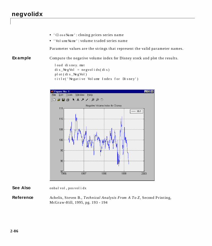
negvolidx
• ’CloseName’: closing prices series name
• ’VolumeName’: volume traded series name
Parameter values are the strings that represent the valid parameter names.
Example Compute the negative volume index for Disney stock and plot the results.
load disney.matdis_NegVol = negvolidx(dis)plot(dis_NegVol)title(’Negative Volume Index for Disney’)
See Also onbalvol, posvolidx
Reference Achelis, Steven B., Technical Analysis From A To Z, Second Printing, McGraw-Hill, 1995, pg. 193 - 194
2-86
onbalvol
2onbalvolPurpose On-Balance Volume (OBV)
Syntax obv = onbalvol(closep, tvolume)obv = onbalvol([closep tvolume])obvts = onbalvol(tsobj)obvts = onbalvol(tsobj, ParameterName, ParameterValue, ...)
Arguments
Description obv = onbalvol(closep, tvolume) calculates the On-Balance Volume (OBV) from the stock closing price (closep) and volume traded (tvolume) data.
obv = onbalvol([closep tvolume]) accepts a two-column matrix representing the closing price (closep) and volume traded (tvolume), in that order.
obvts = onbalvol(tsobj) calculates the On-Balance Volume from the stock data in the financial time series object tsobj. The object must minimally contain series names Close and Volume. obvts is a financial time series object with the same dates as tsobj and a series named OnBalVol.
obvts = onbalvol(tsobj, ParameterName, ParameterValue, ...) accepts parameter name/ parameter value pairs as input. These pairs specify the name(s) for the required data series if it is different from the expected default name(s). Valid parameter names are:
• ’CloseName’: closing prices series name
• ’VolumeName’: volume traded series name
Parameter values are the strings that represent the valid parameter names.
closep Closing price (vector)
tvolume Volume traded
tsobj Financial time series object
2-87
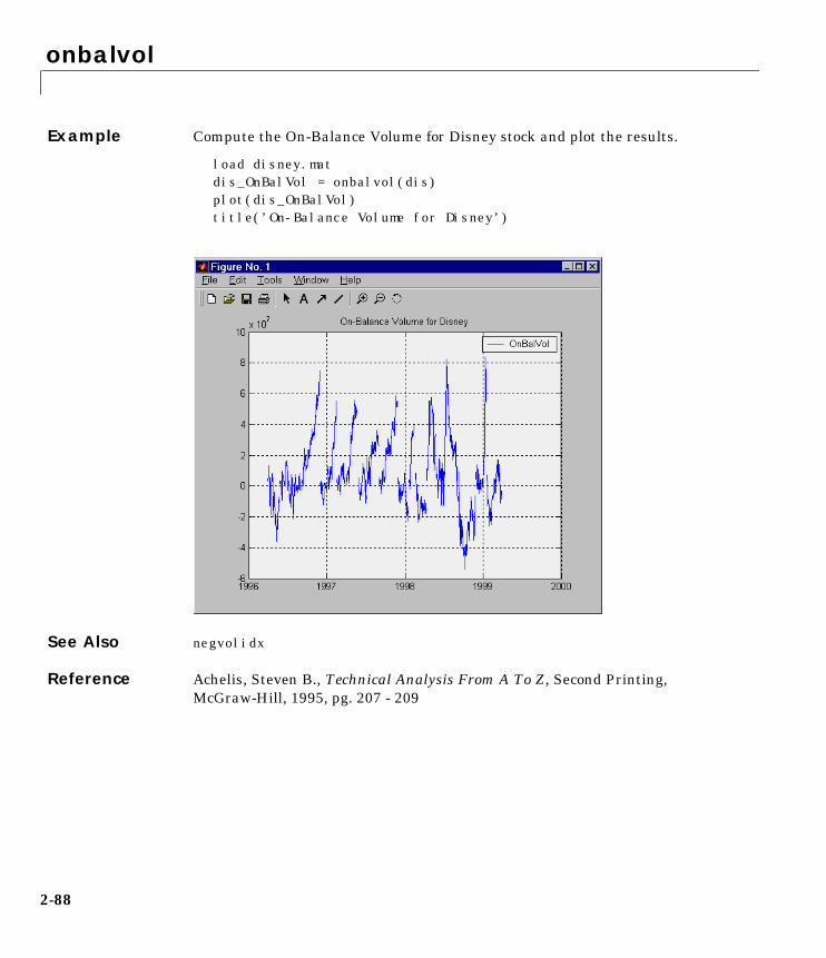
onbalvol
Example Compute the On-Balance Volume for Disney stock and plot the results.
load disney.matdis_OnBalVol = onbalvol(dis)plot(dis_OnBalVol)title(’On-Balance Volume for Disney’)
See Also negvolidx
Reference Achelis, Steven B., Technical Analysis From A To Z, Second Printing, McGraw-Hill, 1995, pg. 207 - 209
2-88
peravg
2peravgPurpose Periodic average
Syntax avgfts = peravg(tsobj, numperiod)avgfts = peravg(tsobj, daterange)
Arguments
Description peravg calculates periodic averages of a financial time series object. Periodic averages are calculated from the values per period defined. If the period supplied is a string, it is assumed as a range of date string. If the period is entered as numeric, the number represents the number of data points (financial time series periods) to be included in a period for the calculation. For example, if you enter ’01/01/98::01/01/99’ as the period input argument, peravg returns the average of the time series between those dates, inclusive. However, if you enter the number 5 as the period input, peravg returns a series of averages from the time series data taken 5 date points (financial time series periods) at a time.
avgfts = peravg(tsobj, numperiod) returns a structure avgfts that contains the periodic (per numperiod periods) average of the financial time series object. avgfts has field names identical to data series names of tsobj.
avgfts = peravg(tsobj, daterange) returns a structure avgfts that contains the periodic (as specified by daterange) average of the financial time series object. avgfts has field names identical to data series names of tsobj.
See Also mean, tsmovavg
mean in the MATLAB documentation
tsobj Financial time series object
numperiod Integer specifying number of data points each periodic average should be averaged over
daterange Time period over which the data is averaged
2-89
plot
2plotPurpose Plot data series
Syntax plot(tsobj)hp = plot(tsobj)plot(tsobj, linefmt)hp = plot(tsobj, linefmt)
Arguments
Description plot(tsobj) plots the data series contained in the object tsobj. Each data series will be a line. plot automatically generates a legend as well as dates on the x-axis. Grid is turned on by default. plot uses the default color order as if plotting a matrix.
hp = plot(tsobj) additionally returns the handle(s) to the object(s) inside the plot figure. If there are multiple lines in the plot, hp is a vector of multiple handles.
plot(tsobj, linefmt) plots the data series in tsobj using format specified. For a list of possible line formats, see plot in the MATLAB documentation. The plot legend will not be generated, but the dates on x-axis and the plot grid will. The specified line format is applied to all data series; that is, all data series can have the same line type.
hp = plot(tsobj, linefmt) additionally plots the data series in tsobj using format specified. The plot legend will not be generated, but the dates on x-axis and the plot grid will. The specified line format is applied to all data series; that is, all data series can have the same line type. If there are multiple lines in the plot, hp is a vector of multiple handles.
Note To turn the legend off, enter legend off at the MATLAB command line. Once you turned it off, the legend is essentially deleted. To turn it back on, recreate it using the legend command as if you are creating it for the first time. To turn the grid off, enter grid off. To turn it back on, enter grid on.
tsobj Financial time series object
linefmt (Optional) Line format
2-90

plot
See Also grid, legend, and plot in the MATLAB documentation
candle, chartfts, highlow
2-91
plus
2plusPurpose Financial time series addition
Syntax newfts = tsobj_1 + tsobj_2newfts = tsobj + arraynewfts = array + tsobj
Arguments
Description minus is an element-by-element addition of the contents of the components.
newfts = tsobj_1 + tsobj_2 adds financial time series objects. If an object is to be added to another object, both objects must have the same dates and data series names, although the order need not be the same. The order of the data series, when one financial time series object is added to another, follows the order of the first object.
newfts = tsobj + array adds an array element-by-element to a financial time series object.
newfts = array + tsobj adds a financial time series object element-by-element to an array.
See Also minus, rdivide, times
tsobj Financial time series object
array A scalar value or array with number of rows equal to the number of dates in tsobj and number of columns equal to the number of data series in tsobj.
2-92
posvolidx
2posvolidxPurpose Positive volume index
Syntax pvi = posvolidx(closep, tvolume, initpvi)pvi = posvolidx([closep tvolume], initpvi)pvits = posvolidx(tsobj)pvits = posvolidx(tsobj, initpvi, ParameterName, ParameterValue, ...)
Arguments
Description pvi = posvolidx(closep, tvolume, initpvi) calculates the positive volume index from a set of stock closing prices (closep) and volume traded (tvolume) data. pvi is a vector representing the positive volume index. If initpvi is specified, posvolidx uses that value instead of the default (100).
pvi = posvolidx([closep tvolume], initpvi) accepts a two-column matrix, the first column representing the closing prices (closep) and the second representing the volume traded (tvolume). If initpvi is specified, posvolidx uses that value instead of the default (100).
pvits = posvolidx(tsobj) calculates the positive volume index from the financial time series object tsobj. The object must contain, at least, the series Close and Volume. pvits is a financial time series object with dates similar to tsobj and a data series named PVI. The initial value for the positive volume index is arbitrarily set to 100.
pvits = posvolidx(tsobj, initpvi, ParameterName, ParameterValue,...) accepts parameter name/ parameter value pairs as input. These pairs specify the name(s) for the required data series if it is different from the expected default name(s). Valid parameter names are:
• ’CloseName’: closing prices series name
• ’VolumeName’: volume traded series name
closep Closing price (vector)
tvolume Volume traded (vector)
initpvi (Optional) Initial value for positive volume index (Default = 100).
tsobj Financial time series object
2-93
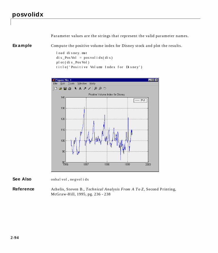
posvolidx
Parameter values are the strings that represent the valid parameter names.
Example Compute the positive volume index for Disney stock and plot the results.
load disney.matdis_PosVol = posvolidx(dis)plot(dis_PosVol)title(’Positive Volume Index for Disney’)
See Also onbalvol, negvolidx
Reference Achelis, Steven B., Technical Analysis From A To Z, Second Printing, McGraw-Hill, 1995, pg. 236 - 238
2-94
power
2powerPurpose Financial time series power
Syntax newfts = tsobj .^ arraynewfts = array .^t sobjnewfts = tsobj_1 .^ tsobj_2
Arguments
Description newfts = tsobj .^ array raises all values in the data series of the financial time series object tsobj element-by-element to the power indicated by the array value. The results are stored in another financial time series object newfts. newfts contains the same data series names as tsobj.
newfts = array .^ tsobj raises the array values element-by-element to the values contained in the data series of the financial time series object tsobj. The results are stored in another financial time series object newfts. newfts contains the same data series names as tsobj.
newfts = tsobj_1 .^ tsobj_2 raises the values in the object tsobj_1 element-by-element to the values in the object tsobj_2. The data series names, the dates, and the number of data points in both series must be identical. newfts contains the same data series names as the original time series objects.
See Also minus, plus, rdivide, times
tsobj Financial time series object
array A scalar value or array with number of rows equal to the number of dates in tsobj and number of columns equal to the number of data series in tsobj.
2-95
prcroc
2prcrocPurpose Price rate of change
Syntax proc = prcroc(closep, nperiods)procts = prcroc(tsobj, nperiods)procts = prcroc(tsobj, nperiods, ParameterName, ParameterValue)
Arguments
Description proc = prcroc(closep, nperiods) calculates the price rate of change proc from the closing price closep. If nperiods periods is specified, the price rate of change is calculated between the current closing price and the closing price nperiods ago.
procts = prcroc(tsobj, nperiods) calculates the price rate of change procts from the financial time series object tsobj. tsobj must contain a data series named Close. The output procts is a financial time series object with similar dates as tsobj and a data series named PriceROC. If nperiods is specified, the price rate of change is calculated between the current closing price and the closing price nperiods ago.
procts = prcroc(tsobj, nperiods, ParameterName, ParameterValue) specifies the name for the required data series when it is different from the default name. The valid parameter name is:
• ’CloseName’: closing price series name
The parameter value is a string that represents the valid parameter name.
closep Closing price
nperiods (Optional) Period difference. (Default = 12.)
tsobj Financial time series object
2-96
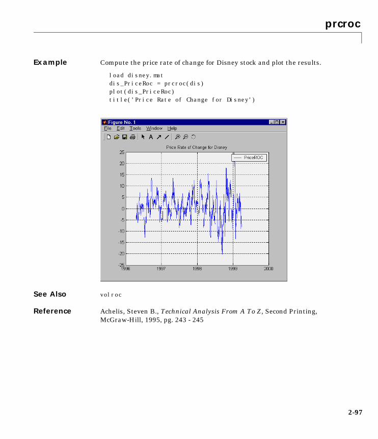
prcroc
Example Compute the price rate of change for Disney stock and plot the results.
load disney.matdis_PriceRoc = prcroc(dis)plot(dis_PriceRoc)title(’Price Rate of Change for Disney’)
See Also volroc
Reference Achelis, Steven B., Technical Analysis From A To Z, Second Printing, McGraw-Hill, 1995, pg. 243 - 245
2-97
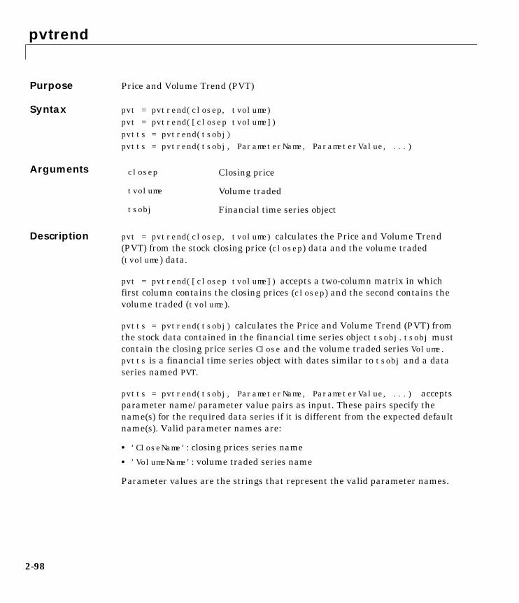
pvtrend
2pvtrendPurpose Price and Volume Trend (PVT)
Syntax pvt = pvtrend(closep, tvolume)pvt = pvtrend([closep tvolume])pvtts = pvtrend(tsobj)pvtts = pvtrend(tsobj, ParameterName, ParameterValue, ...)
Arguments
Description pvt = pvtrend(closep, tvolume) calculates the Price and Volume Trend (PVT) from the stock closing price (closep) data and the volume traded (tvolume) data.
pvt = pvtrend([closep tvolume]) accepts a two-column matrix in which first column contains the closing prices (closep) and the second contains the volume traded (tvolume).
pvtts = pvtrend(tsobj) calculates the Price and Volume Trend (PVT) from the stock data contained in the financial time series object tsobj. tsobj must contain the closing price series Close and the volume traded series Volume. pvtts is a financial time series object with dates similar to tsobj and a data series named PVT.
pvtts = pvtrend(tsobj, ParameterName, ParameterValue, ...) accepts parameter name/ parameter value pairs as input. These pairs specify the name(s) for the required data series if it is different from the expected default name(s). Valid parameter names are:
• ’CloseName’: closing prices series name
• ’VolumeName’: volume traded series name
Parameter values are the strings that represent the valid parameter names.
closep Closing price
tvolume Volume traded
tsobj Financial time series object
2-98

pvtrend
Example Compute the price and volume trend for Disney stock and plot the results.
load disney.matdis_PVTrend = pvtrend(dis)plot(dis_PVTrend)title(’Price and Volume Trend for Disney’)
Reference Achelis, Steven B., Technical Analysis From A To Z, Second Printing, McGraw-Hill, 1995, pg. 239 - 240
2-99

rdivide
2rdividePurpose Financial time series division
Syntax newfts = tsobj_1 ./ tsobj_2newfts = tsobj ./ arraynewfts = array ./ tsobj
Arguments
Description The rdivide method divides element-by-element the components of one financial time series object by the components of the other. You can also divide the whole object by an array or divide a financial time series object into an array.
If an object is to be divided by another object, both objects must have the same dates and data series names, although the order need not be the same. The order of the data series, when an object is divided by another object, follows the order of the first object.
For financial time series objects, the rdivide operation is identical to the mrdivide operation.
See Also minus, mrdivide, plus, times
tsobj Financial time series object
array A scalar value or array with number of rows equal to the number of dates in tsobj and number of columns equal to the number of data series in tsobj.
2-100
resamplets
2resampletsPurpose Downsample data
Syntax newfts = resamplets(oldfts, samplestep)
Description newfts = resamplets(oldfts, samplestep) downsamples the data contained in the financial time series object oldfts every samplestep periods. For example, to have the new financial time series object contain every other data element from oldfts, set samplestep to 2.
newfts is a financial time series object containing the same data series (names) as the input oldfts.
See Also filter
2-101
rmfield
2rmfieldPurpose Remove data series
Syntax fts = rmfield(tsobj, fieldname)
Description fts = rmfield(tsobj, fieldname) removes the data series fieldname and its contents from the financial time series object tsobj. The fieldname must be a cell array to remove multiple data series from the object at the same time. It can be a string array containing the data series name to remove a single series from the object.
See Also chfield, extfield, fieldnames, getfield, isfield
2-102
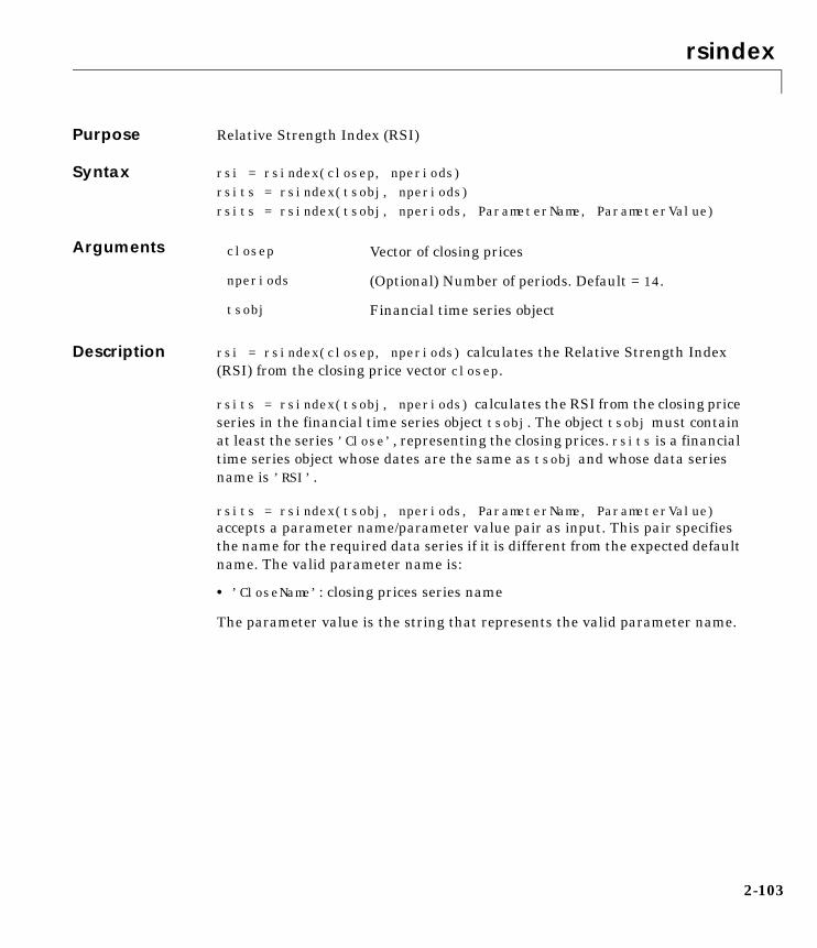
rsindex
2rsindexPurpose Relative Strength Index (RSI)
Syntax rsi = rsindex(closep, nperiods)rsits = rsindex(tsobj, nperiods)rsits = rsindex(tsobj, nperiods, ParameterName, ParameterValue)
Arguments
Description rsi = rsindex(closep, nperiods) calculates the Relative Strength Index (RSI) from the closing price vector closep.
rsits = rsindex(tsobj, nperiods) calculates the RSI from the closing price series in the financial time series object tsobj. The object tsobj must contain at least the series ’Close’, representing the closing prices. rsits is a financial time series object whose dates are the same as tsobj and whose data series name is ’RSI’.
rsits = rsindex(tsobj, nperiods, ParameterName, ParameterValue)accepts a parameter name/parameter value pair as input. This pair specifies the name for the required data series if it is different from the expected default name. The valid parameter name is:
• ’CloseName’: closing prices series name
The parameter value is the string that represents the valid parameter name.
closep Vector of closing prices
nperiods (Optional) Number of periods. Default = 14.
tsobj Financial time series object
2-103
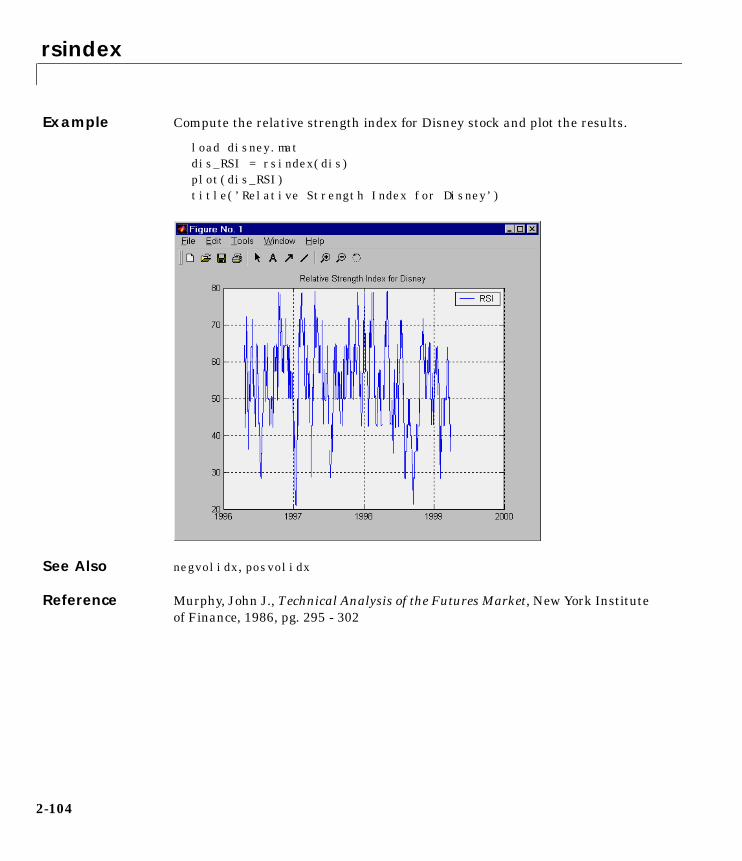
rsindex
Example Compute the relative strength index for Disney stock and plot the results.
load disney.matdis_RSI = rsindex(dis)plot(dis_RSI)title(’Relative Strength Index for Disney’)
See Also negvolidx, posvolidx
Reference Murphy, John J., Technical Analysis of the Futures Market, New York Institute of Finance, 1986, pg. 295 - 302
2-104
setfield
2 setfieldPurpose Set content of a specific field
Syntax newfts = setfield(tsobj, field, V)newfts = setfield(tsobj, field, {dates}, V)
Description setfield treats the contents of fields in a time series object (tsobj) as fields in a structure.
newfts = setfield(tsobj, field, V) sets the contents of the specified field to the value V. This is equivalent to the syntax S.field = V.
newfts = setfield(tsobj, field, {dates}, V) sets the contents of the specified field for the specified dates. dates can be individual cells of date strings or a cell of a date string range using the :: operator, e.g., ’03/01/99::03/31/99’.
Example load dji30short oldfieldnames = fieldnames(myfts1) myfts1 = setfield(myfts1, ’Dividend’, 0.025); newfieldnames = fieldnames(myfts1)
See Also chfield, fieldnames, getfield, isfield, rmfield
2-105

size
2sizePurpose Get number of dates and data series
Syntax szfts = size(tsobj)szfts = size(tsobj, dim)
Arguments
Description szfts = size(tsobj) returns the number of dates (rows) and the number of data series (columns) in the financial time series object tsobj. The result is returned in the vector szfts, whose first element is the number of dates and second is the number of data series.
szfts = size(tsobj, dim) specifies the dimension you want to extract.
See Also size in the MATLAB documentation
length
tsobj Financial time series object
dim Dimension: dim = 1 returns number of dates (rows). dim = 2 returns number of data series (columns).
2-106

smoothts
2smoothtsPurpose Smooth data
Syntax output = smoothts(input)output = smoothts(input, ’b’, wsize)output = smoothts(input, ’g’, wsize, stdev)output = smoothts(input, ’e’, n)
Arguments
Description smoothts smooths the input data using the specified method.
output = smoothts(input) smooths the input data using the default Box method with window size, wsize, of 5.
output = smoothts(input, ’b’, wsize) smooths the input data using the Box (simple, linear) method. wsize specifies the width of the box to be used.
output = smoothts(input, ’g’, wsize, stdev) smooths the input data using the Gaussian Window method.
input input is a financial time series object or a row-oriented matrix. In a row-oriented matrix each row represents an individual set of observations.
’b’, ’g’, or ’e’ Smoothing method (essentially the type of filter used). May be Exponential (e), Gaussian (g), or Box (b). Default = b.
wsize Window size (scalar). Default = 5.
stdev Scalar that represents the standard deviation of the Gaussian window. Default = 0.65.
n For Exponential method, specifies window size or exponential factor, depending upon value.n > 1 (window size) or period length.n < 1 and > 0 (exponential factor: alpha)n = 1 (either window size or alpha)If n is not supplied, the defaults are wsize = 5 and alpha = 0.3333.
2-107
smoothts
output = smoothts(input, ’e’, n) smooths the input data using the Exponential method. n can represent the window size (period length) or alpha. If n > 1, n represents the window size. If 0 < n < 1, n represents alpha, where
If input is a financial time series object, output is a financial time series object identical to input except for contents. If input is a row-oriented matrix, ouput is a row-oriented matrix of the same length.
See Also tsmovavg
α 2wsize 1+-------------------------=
2-108

sortfts
2sortftsPurpose Sort financial time series
Syntax sfts = sortfts(tsobj)sfts = sortfts(tsobj, flag)sfts = sortfts(tsobj, seriesnames, flag)[sfts, sidx] = sortfts(...)
Arguments
Description sfts = sortfts(tsobj, flag) sorts the financial time series object tsobj in increasing order based upon the ’dates’ vector.
sfts = sortfts(tsobj, flag) sets the order of the sort. flag = +1 increases date order. flag = -1 decreases date order.
sfts = sortfts(tsobj, seriesnames, flag) sorts the financial time series object tsobj based upon the data series name(s) seriesnames. If the optional flag is set to -1, the sort is in decreasing order.
[sfts, sidx] = sortfts(...) additionally returns the index of the original object tsobj sorted based on ’dates’ or specified data series name(s).
See Also sort and sortrows in the MATLAB documentation
tsobj Financial time series object
seriesnames (Optional) String containing a data series name or cell array containing a list of data series names
flag (Optional) Sort order:flag = 1; increasing order (default)flag = -1; decreasing order
2-109
spctkd
2spctkdPurpose Slow stochastics
Syntax [spctk, spctd] = spctkd(fastpctk, fastpctd)[spctk, spctd] = spctkd([fastpctk fastpctd]) [spctk, spctd] = spctkd(fastpctk, fastpctd, dperiods, dmamethod)[spctk, spctd] = spctkd([fastpctk fastpctd], dperiods, dmamethod)skdts = spctkd(tsobj) skdts = spctkd(tsobj, dperiods, dmamethod)skdts = spctkd(tsobj, dperiods, dmamethod, ParameterName, ParameterValue, ...)
Arguments
Description [spctk, spctd] = spctkd(fastpctk, fastpctd) calculates the slow stochastics S%K and S%D. spctk and spctd are column vectors representing the respective slow stochastics.
[spctk, spctd] = spctkd([fastpctk fastpctd]) accepts a two-column matrix as input. The first column contains the fast stochastic F%K values, and the second contains the fast stochastic F%D values.
[spctk, spctd] = spctkd(fastpctk, fastpctd, dperiods, dmamethod)calculates the slow stochastics, S%K and S%D, using the value of dperiods to set the number of periods and dmamethod to indicate the moving average method. The inputs fastpctk and fastpctk must contain the fast stochastics, F%K and F%D in column orientation. spctk and spctd are column vectors representing the respective slow stochastics.
Valid moving average methods for %D are Exponential (’e’) and Triangular (’t’). See tsmovavg for explanations of these methods.
fastpctk Fast stochastic F%K (vector)
fastpctk Fast stochastic F%D (vector)
dperiods (Optional) %D periods. Default = 3.
dmamethod (Optional) %D moving average method. Default = ’e’ (exponential).
tsobj Financial time series object
2-110
spctkd
[spctk, spctd] = spctkd([fastpctk fastpctd], dperiods, dmamethod) accepts a two-column matrix rather than two separate vectors. The first column contains the F%K values, and the second contains the F%D values.
skdts = spctkd(tsobj) calculates the slow stochastics, S%K and S%D. tsobj must contain the fast stochastics, F%K and F%D, in data series named PercentK and PercentD. skdts is a financial time series object with the same dates as tsobj. Within tsobj the two series SlowPctK and SlowPctD represent the respective slow stochastics.
skdts = spctkd(tsobj, dperiods, dmamethod) allows you to specify the length and the method of the moving average used to calculate S%D values.
skdts = spctkd(tsobj, dperiods, dmamethod, ParameterName, ParameterValue, ...) accepts parameter name/parameter value pairs as input. These pairs specify the name(s) for the required data series if it is different from the expected default name(s). Valid parameter names are:
• ’KName’: F%K series name
• ’DName’: F%D series name
Parameter values are the strings that represent the valid parameter names.
2-111
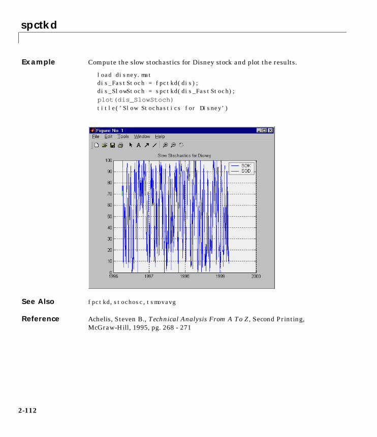
spctkd
Example Compute the slow stochastics for Disney stock and plot the results.
load disney.matdis_FastStoch = fpctkd(dis); dis_SlowStoch = spctkd(dis_FastStoch);plot(dis_SlowStoch)title(’Slow Stochastics for Disney’)
See Also fpctkd, stochosc, tsmovavg
Reference Achelis, Steven B., Technical Analysis From A To Z, Second Printing, McGraw-Hill, 1995, pg. 268 - 271
2-112
std
2stdPurpose Standard deviation
Syntax tsstd = std(tsobj)tsstd = std(tsobj, flag)
Arguments
Description tsstd = std(tsobj) computes the standard deviation of each data series in the financial time series object tsobj and returns the results in tsstd. tsstd is a structure with field name(s) identical to the data series name(s).
tsstd = std(tsobj, flag) normalizes the data as indicated by flag.
See Also hist, mean
tsobj Financial time series object
flag (Optional) Normalization factor:flag = 1 normalizes by N (number of observations).flag = 0 normalizes by (N-1).
2-113
stochosc
2stochoscPurpose Stochastic oscillator
Syntax stosc = stochosc(highp, lowp, closep)stosc = stochosc([highp lowp closep])stosc = stochosc(highp, lowp, closep, kperiods, dperiods, dmamethod)stosc= stochosc([highp lowp closep], kperiods, dperiods, dmamethod)stoscts = stochosc(tsobj, kperiods, dperiods, dmamethod)stoscts = stochosc(tsobj, kperiods, dperiods, dmamethod,
ParameterName, ParameterValue, ...)
Arguments
Description stosc = stochosc(highp, lowp, closep) calculates the Fast PercentK (F%K) and Fast PercentD (F%D) from the stock price data, highp (high prices), lowp (low prices), and closep (closing prices). stosc is a two-column matrix whose first column is the F%K values and second is the F%D values.
stosc = stochosc([highp lowp closep]) accepts a three-column matrix of high (highp), low (lowp), and closing prices (closep), in that order.
stosc = stochosc(highp, lowp, closep, kperiods, dperiods, dmamethod) calculates Fast PercentK (F%K) and Fast PercentD (F%D) from the stock price data, highp (high prices), lowp (low prices), and closep (closing prices). kperiods sets the %K period. dperiods sets the %D period.
damethod specifies the %D moving average method. Valid moving average methods for %D are Exponential (’e’) and Triangular (’t’). See tsmovavg for explanations of these methods.
highp High price (vector)
lowp Low price (vector)
closep Closing price (vector)
kperiods (Optional) %K periods. Default = 10.
dperiods (Optional) %D periods. Default = 3.
damethod (Optional) %D moving average method. Default = ’e’ (exponential).
tsobj Financial time series object
2-114

stochosc
stosc= stochosc([highp lowp closep], kperiods, dperiods, dmamethod) accepts a three-column matrix of high (highp), low (lowp), and closing prices (closep), in that order.
stoscts = stochosc(tsobj, kperiods, dperiods, dmamethod) calculates the Fast PercentK (F%K) and Fast PercentD (F%D) from the stock price data in the financial time series object tsobj. tsobj must minimally contain the series High (high prices), Low (low prices), and Close (closing prices). stoscts is a financial time series object with similar dates to tsobj and two data series named SOK and SOD.
stoscts = stochosc(tsobj, kperiods, dperiods, dmamethod, ParameterName, ParameterValue, ...) accepts parameter name/ parameter value pairs as input. These pairs specify the name(s) for the required data series if it is different from the expected default name(s). Valid parameter names are:
• ’HighName’: high prices series name
• ’LowName’: low prices series name
• ’CloseName’: closing prices series name
Parameter values are the strings that represent the valid parameter names.
2-115
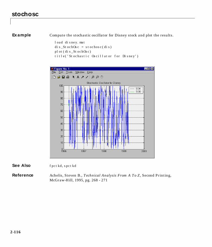
stochosc
Example Compute the stochastic oscillator for Disney stock and plot the results.
load disney.matdis_StochOsc = stochosc(dis) plot(dis_StochOsc)title(’Stochastic Oscillator for Disney’)
See Also fpctkd, spctkd
Reference Achelis, Steven B., Technical Analysis From A To Z, Second Printing, McGraw-Hill, 1995, pg. 268 - 271
2-116
subsasgn
2subsasgnPurpose Content assignment
Description subasgn assigns content to a component within a financial time series object. subasgn supports integer indexing or date string indexing into the time series object with values assigned to the designated components. Serial dates numbers may not be used as indices. To use date string indexing, enclose the date string(s) in a pair of single quotes ’ ’.
You can use integer indexing on the object as in any other MATLAB matrix. It will return the appropriate entry(ies) from the object.
You must specify the component to which you want to assign values. An assigned value must be either a scalar or a column vector.
Example Given a time series myfts with a default data series name of series1.
myfts.series1(’07/01/98::07/03/98’) = [1 2 3]’;
assigns the values 1, 2, and 3 corresponding to the first three days of July, 1998.
myfts(’07/01/98::07/05/98’)
ans =
desc: Data Assignment freq: Daily (1)
’dates: (5)’ ’series1: (5)’’01-Jul-1998’ [ 1]’02-Jul-1998’ [ 2]’03-Jul-1998’ [ 3]’04-Jul-1998’ [ 4561.2]’05-Jul-1998’ [ 5612.3]
See Also datestr in the Financial Toolbox User’s Guide, subsref
2-117

subsref
2subsrefPurpose Subscripted reference
Description subsref implements indexing for a financial time series object. Integer indexing or date string indexing is allowed. Serial dates numbers may not be used as indices.
To use date string indexing, enclose the date string(s) in a pair of single quotes ’ ’.
You can use integer indexing on the object as in any other MATLAB matrix. It will return the appropriate entry(ies) from the object.
Additionally, subsref lets you access the individual components of the object using the structure syntax.
Examples Create a time series named myfts.
myfts = fints((datenum(’07/01/98’):datenum(’07/01/98’)+4)’,... [1234.56; 2345.61; 3456.12; 4561.23; 5612.34], [], ’Daily’,... ’Data Reference’);
Extract the data for the single day July 1, 1998.
myfts(’07/01/98’)
ans =
desc: Data Referencefreq: Daily (1)
’dates: (1)’ ’series1: (1)’’01-Jul-1998’ [ 1234.6]
2-118

subsref
Now, extract the data for the range of dates July 1, 1998 through July 5, 1998.
myfts(’07/01/98::07/03/98’)
ans =
desc: Data Reference freq: Daily (1)
’dates: (3)’ ’series1: (3)’’01-Jul-1998’ [ 1234.6]’02-Jul-1998’ [ 2345.6]’03-Jul-1998’ [ 3456.1]
You can use the MATLAB structure syntax to access the individual components of a financial time series object. To get the description field of myfts, enter
myfts.desc
at the command line, which returns
ans =Data Reference
Similarly
myfts.series1
returns
ans =
desc: Data Reference freq: Daily (1)
’dates: (5)’ ’series1: (5)’’01-Jul-1998’ [ 1234.6]’02-Jul-1998’ [ 2345.6]’03-Jul-1998’ [ 3456.1]’04-Jul-1998’ [ 4561.2]’05-Jul-1998’ [ 5612.3]
2-119

subsref
See Also datestr in the Financial Toolbox User’s Guide.
fts2mtx, subsasgn
2-120
times
2timesPurpose Financial time series multiplication
Syntax newfts = tsobj_1 .* tsobj_2newfts = tsobj .* arraynewfts = array .* tsobj
Arguments
Description The times method multiplies element-by-element the components of one financial time series object by the components of the other. You can also multiply the entire object by an array.
If an object is to be multiplied by another object, both objects must have the same dates and data series names, although the order need not be the same. The order of the data series, when an object is multiplied by another object, follows the order of the first object.
For financial time series objects, the times operation is identical to the mtimes operation.
See Also minus, mtimes, plus, rdivide
tsobj Financial time series object
array A scalar value or array with number of rows equal to the number of dates in tsobj and number of columns equal to the number of data series in tsobj.
2-121
toannual
2toannualPurpose Convert to annual
Syntax newfts = toannual(oldfts)
Description newfts = toannual(oldfts) converts a financial time series of any frequency to one of an annual frequency. toannual sets the dates to the end of the year (December 31).
See Also convertto, todaily, tomonthly, toquarterly, tosemi, toweekly
2-122
todaily
2todailyPurpose Convert to daily
Syntax newfts = todaily(oldfts)
Description newfts = todaily(oldfts) converts a financial time series of any frequency to one of a daily frequency. todaily assumes a five day business week. If oldfts contains weekend data, todaily removes that data when creating newfts.
To create a daily time series from non-daily oldfts, todaily copies the periodic value for however many days there are in the period of the input time series. For example, if oldfts is a weekly time series, the value for each week is replicated four additional times until the next week’s value is encountered. The process is then repeated for the next week.
See Also convertto, toannual, tomonthly, toquarterly, tosemi, toweekly
2-123

todecimal
2todecimalPurpose Fractional to decimal conversion
Syntax usddec = todecimal(quote, fracpart)
Description usddec = todecimal(quote, fracpart) returns the decimal equivalent, usddec, of a security whose price is normally quoted as a whole number and a fraction (quote). fracpart indicates the fractional base (denominator) with which the security is normally quoted (default = 32).
Example In the Wall Street Journal bond prices are quoted in fractional form based on 32nd. For example, if you see the quoted price is 100:05 it means 100 5/32. To find the equivalent decimal value, enter
usddec = todecimal(100.05)
usddec = 1000.1563
usddec = todecimal(97.04, 16)
usddec =97.2500
Note The convention of using . (period) as a substitute for : (colon) in the input is adopted from Microsoft Excel.
See Also toquoted
2-124
tomonthly
2tomonthlyPurpose Convert to monthly
Syntax newfts = tomonthly(oldfts)
Description newfts = tomonthly(oldfts) converts a financial time series of any frequency to one of a monthly frequency. tomonthly assumes a five day business week, when necessary.
If oldfts is a daily or weekly time series, the monthly values in newfts are the averages of the input daily or weekly values. If oldfts is a quarterly, semiannual, or annual time series, the input values are replicated as many times as necessary to fill the monthly time series.
Dates are set to the end of the months.
See Also convertto, toannual, todaily, toquarterly, tosemi, toweekly
2-125

toquarterly
2toquarterlyPurpose Convert to quarterly
Syntax newfts = toquarterly(oldfts)
Description newfts = toquarterly(oldfts) converts a financial time series of any frequency to one of a quarterly frequency. toquarterly assumes a five day business week, when necessary.
If oldfts is a daily, weekly, or monthly time series, the quarterly values in newfts are the averages of the input values for the quarter. If oldfts is a semiannual or annual time series, the input values are replicated as many times as necessary to fill the quarterly time series.
Dates in newfts are set to the end of the quarters (March 31, June 30, September 30, and December 31.
See Also convertto, toannual, todaily, tomonthly, tosemi, toweekly
2-126
toquoted
2toquotedPurpose Decimal to fractional conversion
Syntax quote = toquoted(usddec, fracpart)
Description quote = toquoted(usddec, fracpart) returns the fractional equivalent, quote, of the decimal figure, usddec, based on the fractional base (denominator), fracpart. The fractional bases are the ones used for quoting equity prices in the United States (denominator 2, 4, 8, 16, or 32). If fracpart is not entered, the denominator 32 is assumed.
Example A United States equity price in decimal form is 101.625. To convert this to fractional form in eights of a dollar:
quote = toquoted(101.625, 8)
quote =101.05
The answer is interpreted as 101 5/8.
Note The convention of using . (period) as a substitute for : (colon) in the output is adopted from Microsoft Excel.
See Also todecimal
2-127
tosemi
2tosemiPurpose Convert to semiannual
Syntax newfts = tosemi(oldfts)
Description newfts = tosemi(oldfts) converts a financial time series of any frequency to one of a semiannual frequency. tosemi sets the dates to the end of each semiannual time period (June 30 and December 31).
See Also convertto, toannual, todaily, tomonthly, toquarterly, toweekly
2-128
toweekly
2toweeklyPurpose Convert to weekly
Syntax newfts = toweekly(oldfts)
Description newfts = toweekly(oldfts) converts a financial time series of any frequency to one of a weekly frequency. toweekly assumes a five day business week, when necessary. All days in newfts are set to Fridays.
If oldfts is a daily series, newfts is a financial time series containing data for Fridays only. If oldfts is a monthly, quarterly, semiannual, or annual time series, the input values are replicated as many times as there are Fridays to fill the weekly time series.
See Also convertto, toannual, todaily, tomonthly, toquarterly, tosemi
2-129

tsaccel
2tsaccelPurpose Acceleration between periods
Syntax acc = tsaccel(data, nperiods, datatype)accts = tsaccel(tsobj, nperiods, datatype)
Arguments
Description acc = tsaccel(data, nperiods, datatype) calculates the acceleration of a data series, essentially the difference of the current momentum with the momentum some number of periods ago. If nperiods is specified, tsaccel calculates the acceleration of a data series data with time distance of nperiods periods.
accts = tsaccel(tsobj, nperiods, datatype) calculates the acceleration of the data series in the financial time series object tsobj, essentially the difference of the current momentum with the momentum some number of periods ago. Each data series in tsobj is treated individually. accts is a financial time series object with similar dates and data series names as tsobj.
data Data series
nperiods (Optional) Number of periods. Default = 12.
datatype (Optional) Indicates whether data contains the data itself or the momentum of the data:0 = data contains the data itself (default).1 = data contains the momentum of the data.
tsobj Name of an existing financial time series object
2-130
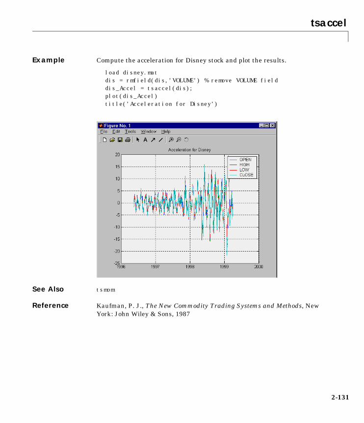
tsaccel
Example Compute the acceleration for Disney stock and plot the results.
load disney.matdis = rmfield(dis,’VOLUME’) % remove VOLUME fielddis_Accel = tsaccel(dis); plot(dis_Accel)title(’Acceleration for Disney’)
See Also tsmom
Reference Kaufman, P. J., The New Commodity Trading Systems and Methods, New York: John Wiley & Sons, 1987
2-131

tsmom
2tsmomPurpose Momentum between periods
Syntax mom = tsmom(data, nperiods)momts = tsmom(tsobj, nperiods)
Arguments
Description Momentum is the difference between two prices (data points) separated by a number of periods.
mom = tsmom(data, nperiods) calculates the momentum of a data series data. If nperiods is specified, tsmom uses that value instead of the default 12.
momts = tsmom(tsobj, nperiods) calculates the momentum of all data series in the financial time series object tsobj. Each data series in tsobj is treated individually. momts is a financial time series object with similar dates and data series names as tsobj. If nperiods is specified, tsmom uses that value instead of the default 12.
data Data series
nperiods (Optional) Number of periods. Default = 12.
tsobj Name of an existing financial time series object
2-132
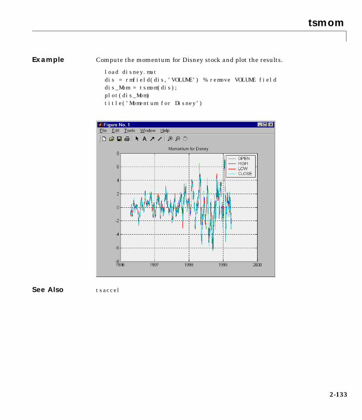
tsmom
Example Compute the momentum for Disney stock and plot the results.
load disney.matdis = rmfield(dis,’VOLUME’) % remove VOLUME fielddis_Mom = tsmom(dis); plot(dis_Mom)title(’Momentum for Disney’)
See Also tsaccel
2-133

tsmovavg
2tsmovavgPurpose Moving average
Syntax output = tsmovavg(tsobj, ’s’, lead, lag) (Simple)output = tsmovavg(vector, ’s’, lead, lag, dim)output = tsmovavg(tsobj, ’e’, timeperiod) (Exponential)output = tsmovavg(vector, ’e’, timeperiod, dim)output = tsmovavg(tsobj, ’t’, numperiod) (Triangular)output = tsmovavg(vector, ’t’, numperiod, dim)output = tsmovavg(tsobj, ’w’, weights, pivot) (Weighted) output = tsmovavg(vector, ’w’, weights, pivot, dim) output = tsmovavg(tsobj, ’m’, numperiod) (Modified)output = tsmovavg(vector, ’m’, numperiod, dim)
Arguments
Description output = tsmovavg(tsobj, ’s’, lead, lag) and output = tsmovavg(vector, ’s’, lead, lag, dim) compute the simple moving average. lead and lag indicate the number of previous and following data points used in conjunction with the current data point when calculating
tsobj Financial time series object
lead Number of following data points
lag Number of previous data points
vector Row vector or row-oriented matrix. Each row is a set of observations.
dim (Optional) Specifies dimension when input is a vector or matrix. Default = 2 (row-oriented). If dim = 1, input is assumed to be a column vector or column-oriented matrix (each column being a set of observations.) output is identical in format to input.
timeperiod Length of time period
numperiod Number of periods considered
weights Weights for each element in the window
pivot Point where the average should be placed
2-134
tsmovavg
the moving average. For example, if you want to calculate a five-day moving average, with the current data in the middle, you set both lead and lag to 2 (2 + 1 + 2 = 5).
output = tsmovavg(tsobj, ’e’, timeperiod) and output = tsmovavg(vector, ’e’, timeperiod, dim) compute the exponential weighted moving average. The exponential moving average is a weighted moving average with the assigned weights decreasing exponentially as you go further into the past. If α is a smoothing constant, the most recent value of the time series is weighted by α, the next most recent value is weighted by α(1-α), the next value by α(1-α)2, and so forth. Here, α is calculated using 2/(timeperiod+1), or 2/(Windows_size+1).
output = tsmovavg(tsobj, ’t’, numperiod) andoutput = tsmovavg(vector, ’t’, numperiod, dim) compute the triangular moving average. The triangular moving average double smooths the data.
tsmovavg calculates the first simple moving average with window width of numperiod/2. If numperiod is an odd number, it rounds up (numperiod/2) and uses it to calculate both the first and the second moving average. The second moving average a simple moving average of the first moving average. If numperiod is an even number, tsmovavg calculates the first moving average using width (numperiod/2) and the second moving average using width (numperiod/2)+1.
output = tsmovavg(tsobj, ’w’, weights, pivot) andoutput = tsmovavg(vector, ’w’, weights, pivot, dim) calculate the moving average by supplying weights for each element in the moving window. The length of the weight vector determines the size of the window. For example, if weights = [1 1 1 1 1] and pivot = 3, tsmovavg calculates a simple moving average by averaging the current value with the two previous and two following values.
output = tsmovavg(tsobj, ’m’, numperiod) andoutput = tsmovavg(vector, ’m’, numperiod, dim) calculate the modified moving average. The first moving average value is calculated by averaging the past numperiod inputs. The rest of the moving average values are calculated by adding to the previous moving average value the current data point divided by numperiod and subtracting the previous moving average divided by numperiod.
2-135

tsmovavg
Moving average values prior to numperiod-th value are copies of the data values.
See Also mean, peravg
Reference Achelis, Steven B., Technical Analysis From A To Z, Second Printing, McGraw-Hill, 1995, pg. 184-192
2-136
typprice
2typpricePurpose Typical price
Syntax tprc = typprice(highp, lowp, closep)tprc = typprice([highp lowp closep])tprcts = typprice(tsobj)tprcts = typprice(tsobj, ParameterName, ParameterValue, ...)
Arguments
Description tprc = typprice(highp, lowp, closep) calculates the typical prices tprc from the high (highp), low (lowp), and closing (closep) prices. The typical price is the average of the high, low, and closing prices for each period.
tprc = typprice([highp lowp closep]) accepts a three-column matrix as the input rather than two individual vectors. The columns of the matrix represent the high, low, and closing prices, in that order.
tprcts = typprice(tsobj) calculates the typical prices from the stock data contained in the financial time series object tsobj. The object must contain, at least, the High, Low, and Close data series. The typical price is the average of the closing price plus the high and low prices. tprcts is a financial time series object of the same dates as tsobj containing the data series TypPrice.
tprcts = typprice(tsobj, ParameterName, ParameterValue, ...)accepts parameter name/ parameter value pairs as input. These pairs specify the name(s) for the required data series if it is different from the expected default name(s). Valid parameter names are:
• ’HighName’: high prices series name
• ’LowName’: low prices series name
• ’CloseName’: closing prices series name
Parameter values are the strings that represent the valid parameter names.
highp High price (vector)
lowp Low price (vector)
closep Closing price (vector)
tsobj Financial time series object
2-137

typprice
Example Compute the typical price for Disney stock and plot the results.
load disney.matdis_Typ = typprice(dis); plot(dis_Typ)title(’Typical Price for Disney’)
See Also medprice, wclose
Reference Achelis, Steven B., Technical Analysis From A To Z, Second Printing, McGraw-Hill, 1995, pg. 291 - 292
2-138

uminus
2uminusPurpose Unary minus of financial time series object
Syntax uminus
Description uminus implements unary minus for a financial time series object.
See Also uplus
2-139
uplus
2uplusPurpose Unary plus of financial time series object
Syntax uplus
Description uplus implements unary plus for a financial time series object.
See Also uminus
2-140
vertcat
2vertcatPurpose Concatenate financial time series objects vertically
Syntax newfts = vertcat(series1, series2, ...)
Description vertcat implements vertical concatenation of financial time series objects. vertcat essentially adds data points to a time series object. The objects to be vertically concatenated must not have any identical dates. However, they must have the same data series names.
The description fields will be concatenated as well. They will be separated by || .
See Also horzcat
2-141

volroc
2volrocPurpose Volume rate of change
Syntax vroc = volroc(tvolume nperiods)vrocts = volroc(tsobj, nperiods)vrocts = volroc(tsobj, nperiods, ParameterName, ParameterValue)
Arguments
Description vroc = volroc(tvolume nperiods) calculates the volume rate of change, vroc, from the volume traded data tvolume. If nperiods periods is specified, the volume rate of change is calculated between the current volume and the volume nperiods ago.
vrocts = volroc(tsobj, nperiods) calculates the volume rate of change, vrocts, from the financial time series object tsobj. vrocts is a financial time series object with similar dates as tsobj and a data series named VolumeROC. If nperiods periods is specified, the volume rate of change is calculated between the current volume and the volume nperiods ago.
vrocts = volroc(tsobj, nperiods, ParameterName, ParameterValue)specifies the name for the required data series when it is different from the default name. The valid parameter name is:
• ’VolumeName’: volume traded series name
The parameter value is a string that represents the valid parameter name.
tvolume Volume traded
nperiods (Optional) Period difference. (Default = 12.)
tsobj Financial time series object
2-142
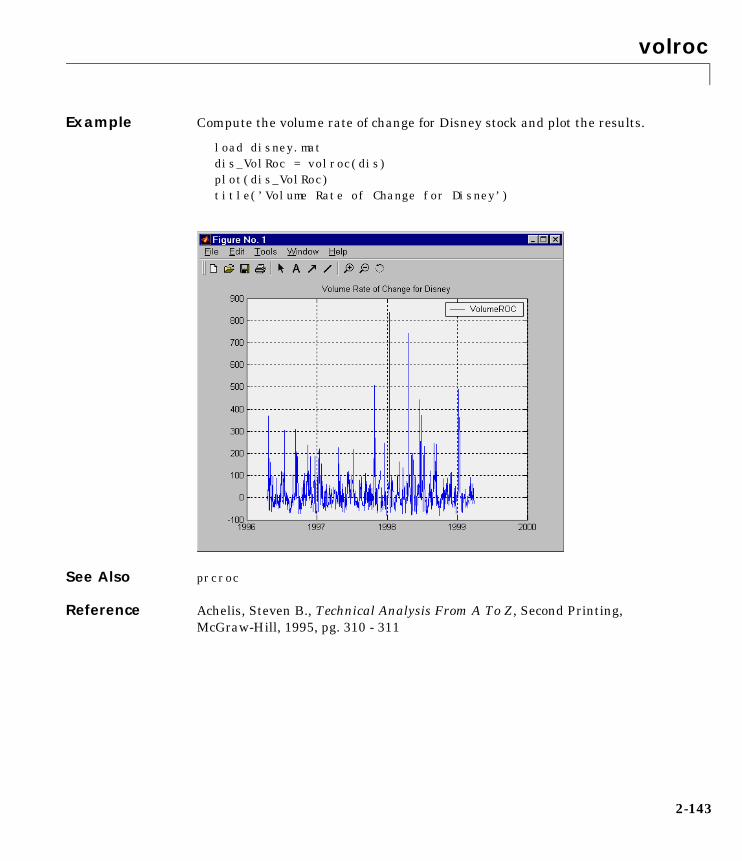
volroc
Example Compute the volume rate of change for Disney stock and plot the results.
load disney.matdis_VolRoc = volroc(dis)plot(dis_VolRoc)title(’Volume Rate of Change for Disney’)
See Also prcroc
Reference Achelis, Steven B., Technical Analysis From A To Z, Second Printing, McGraw-Hill, 1995, pg. 310 - 311
2-143
wclose
2wclosePurpose Weighted close
Syntax wcls = wclose(highp, lowp, closep)wcls = wclose([highp lowp closep])wclsts = wclose(tsobj)wclsts = wclose(tsobj, ParameterName, ParameterValue, ...)
Arguments
Description The weighted close price is the average of twice the closing price plus the high and low prices.
wcls = wclose(highp, lowp, closep) calculates the weighted close prices wcls based on the high (highp), low (lowp), and closing (closep) prices per period.
wcls = wclose([highp lowp closep]) accepts a three-column matrix consisting of the high, low, and closing prices, in that order.
wclsts = wclose(tsobj) computes the weighted close prices for a set of stock price data contained in the financial time series object tsobj. The object must contain the high, low, and closing prices needed for this function. The function assumes that the series are named ’High’, ’Low’, and ’Close’. All three are required. wclsts is a financial time series object of the same dates as tsobj and contains the data series named ’WClose’.
wclsts = wclose(tsobj, ParameterName, ParameterValue, ...) accepts parameter name/parameter value pairs as input. These pairs specify the name(s) for the required data series if it is different from the expected default name(s). Valid parameter names are:
• ’HighName’: high prices series name
• ’LowName’: low prices series name
highp High price (vector)
lowp Low price (vector)
closep Closing price (vector)
tsobj Financial time series object
2-144

wclose
• ’CloseName’: closing prices series name
Parameter values are the strings that represent the valid parameter names.
Example Compute the weighted closing prices for Disney stock and plot the results.
load disney.matdis_Wclose = wclose(dis)plot(dis_Wclose)title(’Weighted Closing Prices for Disney’)
See Also medprice, typprice
Reference Achelis, Steven B., Technical Analysis From A To Z, Second Printing, McGraw-Hill, 1995, pg. 312 - 313
2-145
willad
2willadPurpose William’s Accumulation/Distribution line
Syntax wadl = willad(highp, lowp, closep)wadl = willad([highp lowp closep]) wadlts = willad(tsobj) wadlts = willad(tsobj, ParameterName, ParameterValue, ...)
Arguments
Description wadl = willad(highp, lowp, closep) computes the William’s Accumulation/Distribution line for a set of stock price data. The prices needed for this function are the high (highp), low (lowp), and closing (closep) prices. All three are required.
wadl = willad([highp lowp closep]) accepts a three column matrix of prices as input. The first column contains the high prices, the second contains the low prices, and the third contains the closing prices.
wadlts = willad(tsobj) computes the William’s Accumulation/Distribution line for a set of stock price data contained in the financial time series object tsobj. The object must contain the high, low, and closing prices needed for this function. The function assumes that the series are named High, Low, and Close. All three are required. wadlts is a financial time series object with the same dates as tsobj and a single data series named ’WillAD’.
wadlts = willad(tsobj, ParameterName, ParameterValue, ...) accepts parameter name/parameter value pairs as input. These pairs specify the name(s) for the required data series if it is different from the expected default name(s). Valid parameter names are:
• ’HighName’: high prices series name
• ’LowName’: low prices series name
• ’CloseName’: closing prices series name
highp High price (vector)
lowp Low price (vector)
closep Closing price (vector)
tsobj Time series object
2-146
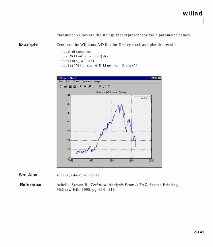
willad
Parameter values are the strings that represent the valid parameter names.
Example Compute the Williams A/D line for Disney stock and plot the results.
load disney.matdis_Willad = willad(dis)plot(dis_Willad)title(’Williams A/D Line for Disney’)
See Also adline, adosc, willpctr
Reference Achelis, Steven B., Technical Analysis From A To Z, Second Printing, McGraw-Hill, 1995, pg. 314 - 315
2-147
willpctr
2willpctrPurpose William’s %R
Syntax wpctr = willpctr(highp, lowp, closep, nperiods)wpctr = willpctr([highp, lowp, closep], nperiods)wpctrts = willpctr(tsobj)wpctrts = willpctr(tsobj, nperiods)wpctrts = willpctr(tsobj, nperiods, ParameterName, ParameterValue,
... )
Arguments
Description wpctr = willpctr(highp, lowp, closep, nperiods) calculates the William’s %R values for the given set of stock prices for a specified number of periods nperiods. The stock prices needed are the high (highp), low (lowp), and closing (closep) prices. wpctr is a vector that represents the William's %R values from the stock data.
wpctr = willpctr([highp, lowp, closep], nperiods) accepts the price input as a three-column matrix representing the high, low, and closing prices, in that order.
wpctrts = willpctr(tsobj) calculates the William's %R values for the financial time series object tsobj. The object must contain at least three data series named High (high prices), Low (low prices), and Close (closing prices). wpctrts is a financial time series object with the same dates as tsobj and a single data series named ’WillPctR’.
wpctrts = willpctr(tsobj, nperiods) calculates the William's %R values for the financial time series object tsobj for nperiods periods.
highp High price (vector)
lowp Low price (vector)
closep Closing price (vector)
nperiods Number of periods (scalar). Default = 14.
tsobj Financial time series object
2-148
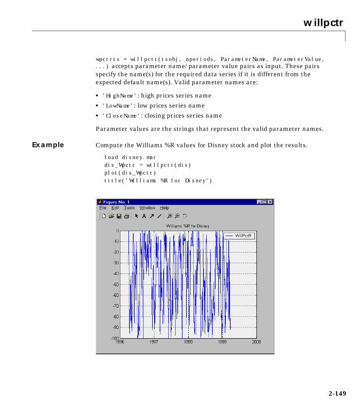
willpctr
wpctrts = willpctr(tsobj, nperiods, ParameterName, ParameterValue, ...) accepts parameter name/ parameter value pairs as input. These pairs specify the name(s) for the required data series if it is different from the expected default name(s). Valid parameter names are:
• ’HighName’: high prices series name
• ’LowName’: low prices series name
• ’CloseName’: closing prices series name
Parameter values are the strings that represent the valid parameter names.
Example Compute the Williams %R values for Disney stock and plot the results.
load disney.matdis_Wpctr = willpctr(dis)plot(dis_Wpctr)title(’Williams %R for Disney’)
2-149
willpctr
See Also stochosc, willad
Reference Achelis, Steven B., Technical Analysis From A To Z, Second Printing, McGraw-Hill, 1995, pg. 316 - 317
2-150
Index
Aadline 2-12adosc 2-15analysis, technical 1-31arithmetic 1-22ascii2fts 1-10, 2-17
Bbollinger 2-18boxcox 1-27, 2-20busdays 2-22
Ccandle 2-23chaikosc 2-25chaikvolat 2-28chartfts 2-31charting 1-31chfield 2-33compatible time series 1-22component 1-13convertto 2-34
Ddata extraction 1-13data series vector 1-13data transformation 1-26date string 1-17
indexing 1-17range 1-19
date vector 1-13datestr 1-17default values 1-13demonstration program 1-39
demonstration time series 2-35demts2fts 2-35description field 1-10, 1-13diff 2-36display 2-37double-colon operator 1-19
Eend 1-22, 2-38equal time series 1-22exp 2-40extfield 2-41extracting data 1-13
Ffieldnames 2-42fillts 2-43filter 2-44fints 2-45
syntaxes 1-3fpctkd 2-47frequency
indicator field 1-13indicators 1-9setting 1-9
frequency conversion 1-26fts2ascii 2-52fts2mtx 1-15, 1-25, 2-53ftsbound 1-20, 2-54ftsdata subdirectory 1-11ftstomtx 2-55
I-1

Index
I-2
Ggetfield 2-55
Hhhigh 2-57highlow 2-59hist 2-61horzcat 2-63
Iindexing
date range 1-19date string 1-17integer 1-20
iscompatible 2-65isequal 2-66isfield 2-67
Llagts 2-68leadts 2-69length 2-70llow 2-71log 2-73log10 2-74
Mmacd 2-75MACD signal line 2-75max 2-77mean 2-78medprice 2-79min 2-81
minus 2-82Moving Average Convergence/Divergence (MACD)
1-33mrdivide 2-83mtimes 2-84
Nnegvolidx 2-85
Oobject structure 1-3On-Balance Volume (OBV) 1-37onbalvol 1-37, 2-87overloaded functions 1-22, 1-30
Pperavg 2-89plot 2-90plus 2-92posvolidx 2-93power 2-95prcroc 2-96pvtrend 2-98
Rrdivide 2-100refield 2-102Relative Strength Index (RSI) 1-36resamplets 2-101rsindex 1-36, 2-103
Sserial dates 1-17
Index
setfield 2-105signal line 2-75size 2-106smoothts 1-29, 2-107sortfts 2-109spctkd 2-110std 2-113stochosc 2-114structures 1-13subsasgn 2-117subsref 2-118
Ttechnical analysis 1-31text file transformation 1-10times 2-121toannual 2-122todaily 2-123todecimal 2-124tomonthly 2-125toquarterly 2-126toquoted 2-127tosemi 2-128toweekly 2-129tsaccel 2-130tsmom 2-132tsmovavg 2-134typprice 2-137
Uuminus 2-139uplus 2-140
Vvertcat 2-141volroc 2-142
Wwclose 2-144willad 2-146Williams %R 1-34willpctr 1-34, 2-148
I-3