finnish fiscal multipliers with a structural var model
TRANSCRIPT

292A Kink that Makes You Sick:The Incentive Effect of Sick Pay on Absence
Petri Böckerman*Ohto Kanninen**Ilpo Suoniemi***
293Finnish fiscal multipliers with a structural VAR model
Markku Lehmus••

Helsinki 2014
* Financial support from Palkansaajasäätiö is gratefully acknowledged.
** Labour Institute for Economic Research. Pitkänsillanranta 3A 6. floor, 00530 Helsinki, Finland. Email: [email protected].
TYÖPAPEREITA 293WORKING PAPERS 293
Palkansaajien tutkimuslaitosPitkänsillanranta 3 A, 00530 HelsinkiPuh. 09−2535 7330Sähköposti: [email protected]
Labour Institute for Economic ResearchPitkänsillanranta 3 A, FI-00530 Helsinki, FinlandTelephone +358 9 2535 7330E-mail: [email protected]
ISBN 978–952–209–130–7 (pdf)ISSN 1795–1801 (pdf)
1
Tiivistelmä
Tutkimus arvioi finanssipolitiikan kertoim(i)en suuruutta rakenteellista VAR-mallia ja suomalaisia
aineistoja hyödyntäen. Tutkimuksen metodologia perustuu hyvin tunnettuun Blanchardin ja Perottin
(2002) artikkeliin. Tutkimuksen perusteella julkisten menojen kerroin on yli yhden suuruinen lyhy-
ellä aikavälillä; verojen kerroin on noin puolet tästä luvusta. Toisin sanoen menojen lisääminen kas-
vattaa bkt:ta itse menolisäykseen käytettyä summaa enemmän lyhyellä aikavälillä. Verojen kerroin-
vaikutus on sen sijaan suurempi pitemmällä aikavälillä. Jatkotarkastelut osoittavat, että menojen
kerroinvaikutus suurenee, kun julkiset investoinnit lasketaan osaksi julkisia menoja. Kerroinesti-
maatteihin sisältyy kuitenkin huomattava määrä epävarmuutta.
Abstract
The financial crisis has given birth to a debate on the effects of fiscal policy on economic activity,
i.e. on fiscal multipliers. While there are now plenty of papers assessing fiscal multipliers for the
U.S., we still have little knowledge about multipliers for economies such as Finland that have many
distinguishable features. This paper estimates fiscal multipliers for the Finnish economy with a
structural VAR model using Finnish data. The methodology of the model used is based on a much
cited study by Blanchard and Perotti (2002). The study finds expenditure multipliers greater than 1
in the short run and tax multipliers half of that value. Nevertheless, tax multipliers are more
persistent in time. With public investments also included in the public expenditure variable, the
expenditure multiplier becomes more persistent.
Keywords: Fiscal policy, fiscal multipliers, VAR models
1. Introduction
The current crisis has lifted fiscal policy to the centre of the economic debate. In addition to issues
related to debt, the debate has also concerned fiscal multipliers, i.e. how much more output can be
achieved with one additional government euro. This has also given birth to multiple research papers
on the topic. The methods of the studies vary from simple one-equation regression models to highly
complex theory-based macro models. Most of the studies have used U.S. data.
2
The literature on fiscal multipliers has been reviewed, for instance, by Auerbach (2012). In general,
the effect of fiscal policy on economic activity has been studied with three different kinds of
models: larger-scale macroeconomic models, dynamic stochastic general equilibrium (DSGE)
models, and structural vector autoregression models (SVARs) and other theoretically simple time
series approaches. Large-scale macro models are based on structural equations that describe the
behaviour of households and firms. Hence they aim to capture the relevant connections between
macro quantities and prices, using econometric techniques and historical data. Most of these are
backward-looking and use error-correction model equations. These kinds of the “old school” type of
models are still widely used in assessing the effects of fiscal policy, although they have been
criticised in the literature due to the lack of micro foundations.
Large-scale macro models typically find relatively large multipliers for fiscal stimulus. The short-
run multipliers for government purchases may be greater than 1 while those for taxes are typically
slightly smaller. For instance, the Obama administration (see Bernstein and Romer 2009) used
standard large-scale macro models to assess the potential effects of the stimulus package aimed at
mitigating the economic consequences of the great recession in the U.S. (the package known as
‘ARRA’). For an increase in government purchases, the models produced a multiplier of 1.5; the
corresponding multiplier for tax cuts was about 1.0.
DSGE models are rigorously based on micro theory and use Bayesian estimation or calibration in
their parameterization. DSGE macro models usually give slightly smaller estimates for fiscal
multipliers than large-scale macro models. Hall (2009) reviews the DSGE literature and concludes
that DSGE models that incorporate certain nominal rigidities in wages and prices, i.e. New
Keynesian features, generate government spending multipliers that are well above zero, but below
1.0. Coenen et al. (2012) use seven structural DSGE models developed in different policymaking
institutions to study the effects of fiscal stimulus. When they examine the effects of government
consumption and assume that no monetary accommodation is done at the same time, the
instantaneous multipliers for the first year range between 0.7 and 1.0 for the United States, and
between 0.8 and 0.9 for Europe. The multipliers naturally become larger if monetary policy is
assumed to be accommodative. Regarding different policy instruments, Coenen et al. find that the
multipliers are greatest for government consumption and targeted transfers. However, while being
theoretically consistent and coherent DSGE models may poorly fit the data.

3
In an SVAR model a vector of variables is explained by lagged values of the same variables. In the
fiscal multiplier literature, a canonical VAR model includes output, taxes and government
purchases. While there is no specification of the channels through which policies affect output, a
limited structure is provided by the assumptions made about the recursive structure of the error
matrix, i.e. the order in which shocks to variables occur. In this way it is possible to identify the
actual changes in current policy variables rather than the endogenous responses to economic
conditions.
A seminal contribution to the SVAR literature is Blanchard & Perotti (2002). They assess the
dynamic effects of shocks in government spending and taxes on U. S. activity in the postwar period.
The identifying assumption in the paper is that spending and taxes could respond to output within a
quarter only through automatic provisions, not discretionary policy. Thus, the fiscal shocks within a
period could be treated as exogenous. As a result, they find multipliers that are close to 1.
Depending on the specification, the spending multiplier is larger or smaller than the tax multiplier.
The effect of taxes on output takes more time to build up.
To improve the identification of policy shocks, the basic SVAR methodology has also been
extended with a narrative approach. In this approach, policy changes have been identified by
applying additional information on policy decisions. The aim of this approach is to capture the truly
exogenous policy shocks. One of the best known papers using this methodology is Romer and
Romer (2010), who use the approach to estimate the effect of tax changes for the U.S. economy.
They find a GDP tax-cut multiplier of about 1.0 after four quarters, even rising to 3.0 after 10 quarters.
This is mainly due to an enormous impact on investments.
One exogenous source of variation with respect to economic activity that has also been used in
studies is military spending build-ups. Ramey (2011a) estimates the effect of these build-ups on
GDP using U.S. data and finds an output multiplier after four quarters of about 0.7. Barro and
Redlick (2011) also use long-term U.S. macroeconomic data and variations in defence spending to
identify spending multipliers. In their study the estimated multiplier for temporary spending is 0.4–
0.5 contemporaneously and 0.6–0.7 over 2 years. If the change in defence spending can be viewed
as permanent, the multipliers are higher by 0.1–0.2. Finally, Ramey (2011b) summarizes the
available evidence on fiscal multipliers and concludes that the multiplier for a temporary, deficit-
financed increase in government purchases is within the range (0.8, 1.5). Nevertheless, she states
that values below and above this range cannot be ruled out.

4
One important contribution to improve the standard SVAR analysis is Auerbach and
Gorodnichenko (2012). They extend the previous studies by using real-time forecasts of taxes,
government purchases and GDP, in order to make the purified shocks correspond more closely to
true stochastic innovations. Secondly and more importantly, they allow multipliers to vary
according the state of the economy. The state of the economy is simply determined with a function
of lagged GDP growth rates. This way they are able to produce the SVAR parameters either for
“recession” or “expansion”. Applying this to quarterly postwar US data, they find that fiscal
multipliers are much larger in recessions than expansions, and that values seem to be above the
upper range of Ramey’s range in recession (i.e. larger than 1.5) but smaller in expansion (smaller
than 0.8).1
In a time-series study, Almunia et al. (2010) find that fiscal multipliers are clearly greater in a
deflationary environment like that of the 1930s or the period through which many countries have
been suffering lately. Blanchard and Leigh (2013) also show that fiscal multipliers have been higher
than predicted in the recent financial crisis. DeLong and Summers (2012), for their part, derive a
theoretical result that in a severely depressed economy at the zero lower bound the government
spending multiplier can even be 2.5.
While there are many studies on fiscal multipliers concerning the U.S., there are almost no
empirical studies for many other countries, including Finland.2 Still, it is clear that the Finnish
economy differs from the U.S. economy with respect to many properties, for instance the size, the
exchange rate regime, the share of exports in output (openness), the size of the public sector, the
labour markets, and the industrial structure. For these reasons, the multipliers gained from studies
using the U.S. data provide little information on fiscal multipliers for Finland.
In this study, I use the methods of the classical study by Blanchard and Perotti (2002) to assess the
fiscal multipliers for the Finnish economy. Thus, I use an SVAR model augmented with dummy
variables to control the Finnish depression at the beginning of the ‘90s to estimate the dynamic
effects of taxes and government consumption on economic activity. I utilize quarterly data that
cover the years 1975-2011. I also use different time dummies to check the robustness of the results.
Finally, I analyze the effects of changes in taxation and government purchases using the
1 This assumption – a non-linear relation between the state of the economy and the fiscal multiplier – is used in a
number of recent papers, e.g. Owyang et al. (2013), Caggiano et al. (2014), and Riera-Crichton et al. (2014). The papers
find somewhat mixed evidence on the effect of economic circumstances on the fiscal multiplier. 2 There is only one study that ought to be mentioned here: Kuismanen and Kämppi (2010).

5
macroeconometric model (EMMA) developed at the Labour Institute for Economic Research.
These results are compared with the results gained from the SVAR model specification.
2. Methodology
The analysis utilizes the SVAR model methodology à la Blanchard and Perotti (2002), later referred
to in this paper as B-P. A natural assumption to begin with is that shocks in both taxation and
government expenditure affect economic activity. In this study, government expenditures consist of
public consumption, which covers the consumption expenditures of the central government,
municipalities, and the social security funds. In the baseline specification I exclude public
investments from the model structure, since their effects are assumed to differ from those of
government consumption. Yet later on, I use another specification of the model in which public
investments are also included in the public expenditure variable which, in fact, is how B-P construct
the variable. Taxes, or “revenues”, are defined as the total amount of taxes collected by the public
sector. Thus, the variable consists of a variety of different tax forms, ranging from income taxes
paid by individuals to corporate taxes paid by firms.
The VAR model has a well-known structure, which is the following:
(1) 1( , )t t t
Y A L q Y U−
= +
In this specification [ ], , 't t t tY T G X≡ . Hence the vector Y constitutes taxes (revenues) (T ), public
consumption (G ), and output ( X ). Following B-P, the identification strategy used here requires
the use of quarterly data.3 ( ),A L q is a four-quarter distributed lag polynomial that allows for
quarter-dependence of the coefficients. This polynomial is to capture the possible seasonal patterns
in the response of taxes or spending to economic activity. [ ], , 't t t tU t g x≡ is the error term (with
nonzero cross correlations).
3 Note that, in B-P, revenues are taxes minus transfers, referred to as “net taxes”. In this paper, on the other hand, the
variable T denotes “gross taxes”, i.e. transfers are not reduced from the variable.
6
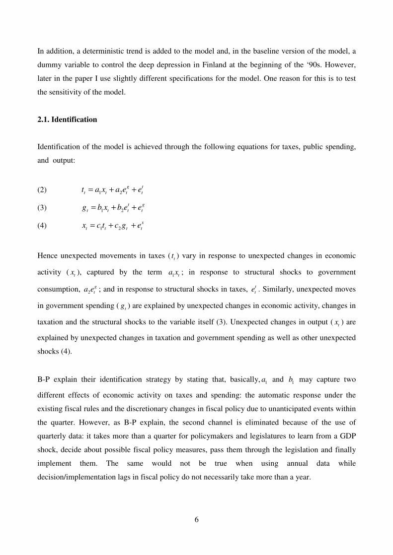
In addition, a deterministic trend is added to the model and, in the baseline version of the model, a
dummy variable to control the deep depression in Finland at the beginning of the ‘90s. However,
later in the paper I use slightly different specifications for the model. One reason for this is to test
the sensitivity of the model.
2.1. Identification
Identification of the model is achieved through the following equations for taxes, public spending,
and output:
(2) 1 2
g t
t t t tt a x a e e= + +
(3) 1 2
t g
t t t tg b x b e e= + +
(4) 1 2
x
t t t tx c t c g e= + +
Hence unexpected movements in taxes (t
t ) vary in response to unexpected changes in economic
activity (t
x ), captured by the term 1 ta x ; in response to structural shocks to government
consumption, 2
g
ta e ; and in response to structural shocks in taxes, t
te . Similarly, unexpected moves
in government spending (t
g ) are explained by unexpected changes in economic activity, changes in
taxation and the structural shocks to the variable itself (3). Unexpected changes in output (t
x ) are
explained by unexpected changes in taxation and government spending as well as other unexpected
shocks (4).
B-P explain their identification strategy by stating that, basically, 1a and 1b may capture two
different effects of economic activity on taxes and spending: the automatic response under the
existing fiscal rules and the discretionary changes in fiscal policy due to unanticipated events within
the quarter. However, as B-P explain, the second channel is eliminated because of the use of
quarterly data: it takes more than a quarter for policymakers and legislatures to learn from a GDP
shock, decide about possible fiscal policy measures, pass them through the legislation and finally
implement them. The same would not be true when using annual data while
decision/implementation lags in fiscal policy do not necessarily take more than a year.

7
With these assumptions, we can simply estimate 1a and 1b , the elasticities of tax revenues and
government spending with respect to output, from quarterly data. First, the estimation gives the
feedback parameter from economic activity to government spending, 1b , the value of 0.4. Hence
government spending and output appear to some extent to co-move in Finland.4 The estimated
elasticity of tax revenues with respect to output, 1a , is then 1.27. The estimate greater than 1 is
mainly due to the progressivity of many taxes, for instance income taxation. Another observation
from the data is that the estimate seems to decrease over time. Thus, if the estimation is done for the
period 1975-1990, the coefficient gets a value of 1.36. This may indicate weakening of the
progressivity of the tax system in time. In addition, the estimate is smaller than the one that B-F
find from the U.S. data.
Estimation of 1c and 2c is done with the help of cyclically adjusted reduced-form tax and spending
residuals. We need these cyclically adjusted reduced-form tax and spending residuals while the
unexpected tax revenues (t
t ) and government spending (t
g ) may correlate with the error term x
te .
To construct these, I use the estimates 1a and 1b so that '
1t t tt t a x= − produces the cyclically
adjusted reduced-form tax residuals and '
1t t tg g b x= − is the spending residuals. The residuals are
then used as instruments to estimate 1c and 2c .
Estimation of 2a and 2b leaves a puzzle: do taxes respond to changes in government spending or
vice versa? When solving the model I need to assume that either 2 0a = or 2 0b = in order the
model to identify. In the Finnish data, there is correlation between cyclically adjusted taxes and
government spending, that is somewhat in contrast to what B-P find with the U.S data. The
correlation is probably due to the behaviour of municipalities while they tend to adjust their
spending if there is a surprise in tax revenues, and vice versa. So these institutions behave
somewhat more endogenously than the central government. Thus, if I assume that spending comes
first, i.e. 2 0b = , the estimation gives 2a a value of 0.59, which implies that there is quite a large
response of taxes to public spending. The opposite hypothesis, that government spending reacts to
tax changes, gives 2b a value of 0.21, which means a somewhat smaller response of government
4 A trend variable is also added to the estimated equation. Note that B-P cannot identify this kind of covariance between
government spending and output in the U.S.
8
spending to taxes. Thus, in the following analysis I simulate the model with both these assumptions,
i.e. either with 2 0.59a = and 2 0b = or 2 0a = and 2 0.21b = .
The parameters are utilized to characterize the dynamic effects of fiscal shocks. While the
parameters represent average elasticities, the computed impulse responses also give the average
dynamic responses to shocks.
3. The Data
I use time-series data for the period 1975-2011. The tax data are from Statistics Finland. Taxes
include all the tax revenues collected by the public sector, consisting of personal income taxes,
social security contribution payments, property taxes, and indirect taxes. Public spending is public
consumption defined by the national accounts. I use a broad definition for the public sector; hence
the central government, municipalities and the social security funds are calculated together. The
public spending series is quarterly and seasonally adjusted by Statistics Finland, but the tax data are
only available on a yearly basis. For that reason, the tax revenues are disaggregated in this paper
using the Ecotrim program. As a reference series for the disaggregation, I use the quarterly wage
sum paid in the economy.
The ratio of tax revenues to nominal GDP is depicted in Figure 1. It can be seen that there was an
upward spike in the tax revenues in 1976. That year, the Finnish government announced 26 different
types of tax hikes, as calculated by the Taxpayers’ Association of Finland. However, taxes fell again
at the end of the 1970s. After that, there was a trend, an increase in taxes, until the middle of the
1990s. The first part of the trend can be seen as an era of building the Finnish Welfare State Model.
The second, on the other hand, can be seen as the government’s austerity measures aimed at balancing
its budget in the middle of the deep depression of the ‘90s. Since the middle of the 1990s there have,
however, been several tax cuts, particularly targeted at the income taxes paid by households.

9
Figure 1. Tax revenues as a share of GDP, %
.32
.34
.36
.38
.40
.42
.44
.46
.48
1975 1980 1985 1990 1995 2000 2005 2010
The share of public spending of nominal GDP is shown in Figure 2. The ratio rose in the 1980s
amid an increasing share of services provided by the public sector. This was followed by the sharp
spike at the beginning of the 1990s when the Finnish economy was hit by a severe depression. After
that, the Finnish government cut public consumption, and, simultaneously, the Finnish economy
started a rapid recovery from the depression, helped by the devaluation of the Finnish currency. In
addition, the recent global financial crisis appears as a sharp rise in the contribution of public
consumption to GDP. This is, however, no surprise, as the Finnish GDP dropped more than 8 per
cent in 2009.
Figure 2. Public spending as a share of GDP, %
.16
.18
.20
.22
.24
.26
1975 1980 1985 1990 1995 2000 2005 2010
10
Thus, our data includes two distinctive periods: A severe depression at the beginning of the 1990s
and the other one, in 2009, that was very deep but not so long-lasting. I shall deal with these major
shocks by first solving the model using dummy variables to isolate the crisis in the 1990s. This is
done by using two different model specifications. Then later on, I shall also solve the model with
dummy variables for both depressions, of the 1990s and 2009.
As regards low-frequency properties of the data, it seems that there is an upward trend both in tax
revenues and public spending, though the trend in tax revenues seems to take an opposite sign after
the middle of the 1990s and the series of tax cuts made then. As is well known in the economics and
statistics literature, it is difficult to distinguish the deterministic and stochastic trends in the data.
The Augmented Dickey Fuller test tells us that our tax revenues series has a unit root, but the public
spending series has not. Fortunately, the results by B-P suggest that assumption of the type of trend
does not drive the model results.
In this paper, the VARs are estimated with an assumption of deterministic trends in variables.
Hence I allow for linear terms in time in each of the equations of the VAR. In addition, the
benchmark model is solved with a time dummy variable for the years 1991 and 1992, representing
the deep depression in Finland at that time.5
4. The effects of fiscal shocks.
4.1. The contemporaneous effects
I begin by analyzing the contemporaneous effects of the shocks. These are given by the estimated
parameter coefficients in equations (2) – (4); they are shown in Table 1. As was said above, I
assume trends in variables to be deterministic. The table reports estimates for both 2a and 2b ; when
solving the model I need to assume that either 2 0a = or 2 0b = . All the estimated coefficients can
be interpreted as elasticities while I have used logarithmic data.
5 To produce reasonable estimates for fiscal multipliers, one needs somehow control this severe depression.

11
Table 1. Contemporaneous relations between variables
1c 2c 2a 2b
Coefficient -0.34 0.20 0.59 0.21
t-value -3.52 1.26 2.74 2.71
p-value <0.01 0.21 <0.01 <0.01
The estimated contemporaneous effect of a tax increase on GDP is -0.34. The estimate is
statistically significantly larger than zero and not in contrast to the previous studies, though the size
of this estimate varies considerably between studies. Note that our parameter only describes the
effect of a tax shock within a quarter; the dynamic effects of a shock are analyzed later in the study.
The estimate for the contemporaneous effect of a government spending shock on GDP is 0.20. This
number is considerably smaller than B-P’s estimate, calculated using the U.S. data. In addition, the
estimate is not statistically significant, which may cause some problems with robustness issues.
However, the analysis of the dynamic effects will show that the effect of the government spending
shock on economic activity comes with a (short) lag. The estimates for 2a and 2b are statistically
significant and, also, their magnitude implies that tax and government spending innovations
correlate in the Finnish data. A further examination of the data indicates that the correlation is 0.35
and it has in fact grown after the 1970s. Thus, it seems that public spending increases have many
times been compensated for in the government (or more likely, municipality) budget by tax hikes,
and vice versa. This also defines the effects of fiscal shocks analyzed in the following section.
4.2. The dynamic effects of the fiscal shocks
4.2.1. The baseline simulations
The model is first solved with an assumption that taxes come first, i.e. 2 0a = , implying that it is
government spending that reacts to changes in taxes. In this case, 2 0.21b = . Also, the benchmark
model includes dummy variables for the deep depression at the beginning of the 1990s. The
simulation results for the benchmark model are shown in Figure 3, which depicts the impulse
responses between all the model variables and structural shocks. The solid lines are the point
estimates, whereas the dashed lines give one-standard deviation bands, computed from Monte Carlo
simulations with 500 replications.

12
Figure 3. The impulse responses of model variables
5 10 15 20
0
0.2
0.4
0.6
0.8R
evenue s
hocks
Revenue
5 10 15 20
-0.5
0
0.5
Spendin
g s
hocks
5 10 15 20-0.15
-0.1
-0.05
Spending
5 10 15 20
0
0.5
1
5 10 15 20
-0.35
-0.3
-0.25
-0.2
-0.15
-0.1
Output
5 10 15 20
-0.2
0
0.2
0.4
0.6
It can be seen that an increase in taxes has a negative effect on GDP. This effect comes with a small
lag but it also stays negative in the long run. On the other hand, an increase in government
consumption has a positive effect on economic activity. The maximum effect comes after five
quarters and it seems to be sharper when compared with the tax change. However, the positive
effect of government spending on economic activity decreases in the long run, which is in fact in
line with many previous international studies.
However, in order to compare the magnitude of the effects of the fiscal shocks, one needs to
calculate the fiscal multipliers. Thus, I scale the impulse responses to give the effect of a one unit
(relative to GDP) increase in taxes or, in the other scenario, government spending, on economic
activity. The multipliers for the fiscal shocks are shown in Figure 4.

13
Figure 4. The multiplier effects of fiscal shocks
0 5 10 15 20 25-1
-0.5
0Tax multiplier
0 5 10 15 20 25-2
0
2
4Expenditure multiplier
Figure 4 shows basically the same as the GDP response lines in Figure 3, but now it is possible to
analyze the sizes of the multipliers while the numbers are appropriately scaled. In addition, the
multipliers for selected quarters with the peak impact are reported in Table 2.
Table 2. The GDP effect of a one unit increase in taxes or public spending
1 qrt 2 qrt 4 qrt 8 qrt 12 qrt 16 qrt 24 qrt Peak
Tax increase -0.29 -0.32 -0.54 -0.62 -0.60 -0.52 -0.36 -0.63 (9)
Spending inc. 0.06 1.10 1.17 1.18 0.59 0.03 0.00 1.30 (5)
From these it can be seen that the tax multiplier is robustly negative and reaches its peak effect in
nine quarters. At that time, a one percentage unit (relative to GDP) increase in taxes reduces GDP
by 0.63 per cent. After six years, the effect is still negative but smaller, -0.36 per cent on GDP. On
the other hand, government consumption has its peak effect on economic activity in five quarters.
Thus, at the beginning of the second year after the shock the one per cent increase in government

14
spending adds GDP by 1.30 per cent. Nevertheless, the effect decreases relatively rapidly and after
three years the multiplier is only 0.59. After that, it continues to dampen and goes to zero.
In the previous case it was assumed that taxes came first, and hence 2 0a = . Nevertheless, while it is
impossible to identify the order of taxes and public spending variables, I next assume, instead, that
taxes respond to changes in public consumption. In that case it is public consumption that comes
first and 2 0b = but 2 0.59a = , as estimated before. The results of the impulse response are shown in
Figure 5. Again, in Figure 6 the GDP responses of the shocks are scaled to give the fiscal
multipliers of the tax and spending shocks. Table 3 reports the exact numbers of these fiscal
multipliers.
Figure 5. The impulse responses of model variable (specification 2)
5 10 15 20
-0.2
0
0.2
0.4
0.6
0.8
Revenue s
hocks
Revenue
5 10 15 20-0.6
-0.4
-0.2
0
0.2
0.4
Spendin
g s
hocks
5 10 15 20
0
0.2
0.4
Spending
5 10 15 20
0
0.2
0.4
0.6
0.8
1
5 10 15 20
-0.4
-0.3
-0.2
-0.1
0
0.1
Output
5 10 15 20
-0.2
0
0.2
0.4
0.6
15
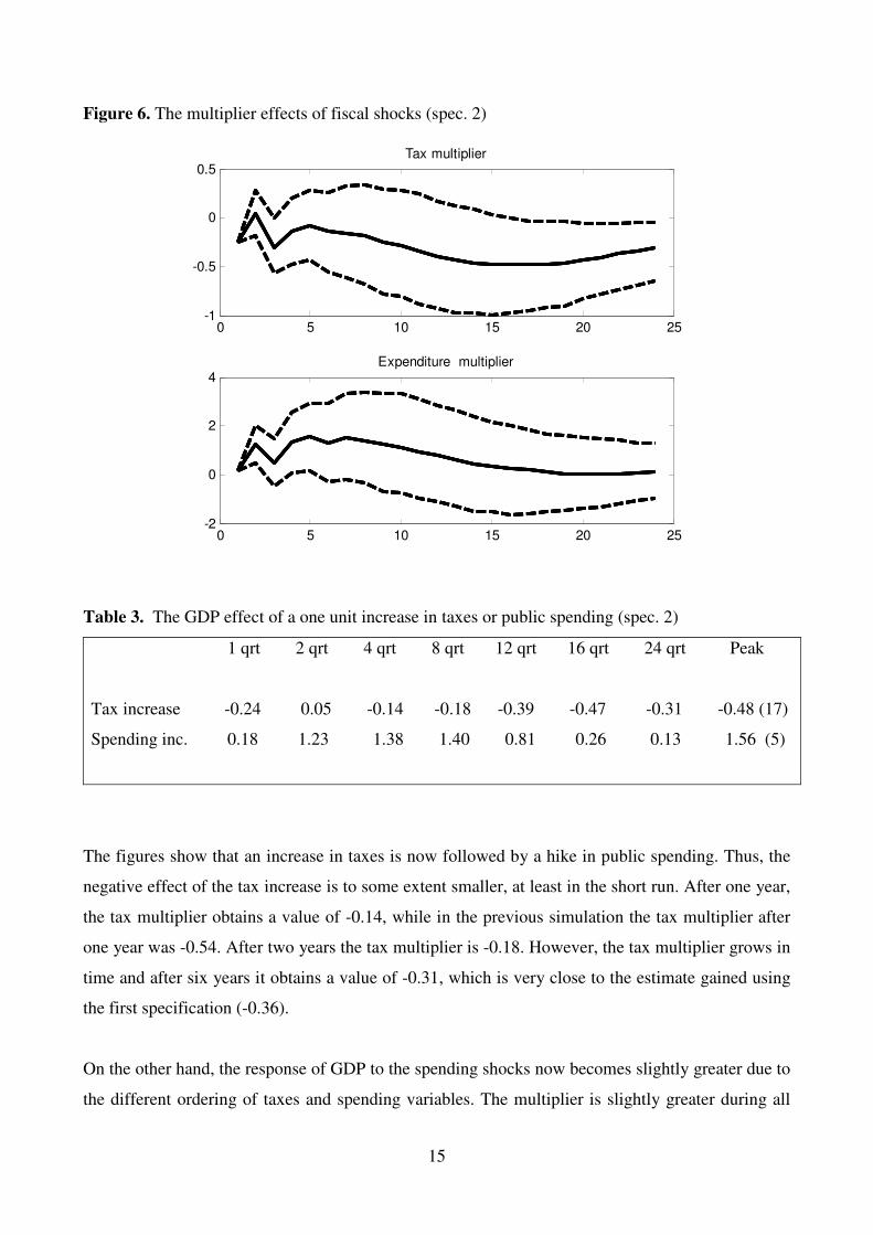
Figure 6. The multiplier effects of fiscal shocks (spec. 2)
0 5 10 15 20 25-1
-0.5
0
0.5Tax multiplier
0 5 10 15 20 25-2
0
2
4Expenditure multiplier
Table 3. The GDP effect of a one unit increase in taxes or public spending (spec. 2)
1 qrt 2 qrt 4 qrt 8 qrt 12 qrt 16 qrt 24 qrt Peak
Tax increase -0.24 0.05 -0.14 -0.18 -0.39 -0.47 -0.31 -0.48 (17)
Spending inc. 0.18 1.23 1.38 1.40 0.81 0.26 0.13 1.56 (5)
The figures show that an increase in taxes is now followed by a hike in public spending. Thus, the
negative effect of the tax increase is to some extent smaller, at least in the short run. After one year,
the tax multiplier obtains a value of -0.14, while in the previous simulation the tax multiplier after
one year was -0.54. After two years the tax multiplier is -0.18. However, the tax multiplier grows in
time and after six years it obtains a value of -0.31, which is very close to the estimate gained using
the first specification (-0.36).
On the other hand, the response of GDP to the spending shocks now becomes slightly greater due to
the different ordering of taxes and spending variables. The multiplier is slightly greater during all

16
the six-year period analyzed here. The peak in the multiplier effect comes after five quarters, when
it reaches a value of 1.56; in the previous simulation, the peak response was 1.30. However, the
fiscal multiplier decreases quite rapidly and after three years it amounts to 0.81. In the long run, the
multiplier is very close to zero. Nevertheless, one observation from all the impulse response figures
is that confidence intervals – even one-standard deviation intervals presented here – are quite wide
and reflect the uncertainty associated with the estimates. One should remember this when reading
the point estimates in Tables 2 and 3.
Even though the data shows correlation between government spending and tax revenue innovations,
I also solve the model with an assumption that the shocks are, instead, independent and non-
correlated, while this is a quite standard assumption in the literature. The results for the fiscal
multiplier are shown in Appendix 1. It comes as no surprise that as regards the tax revenue shock,
the results appear to be as depicted in Figure 4, and with respect to the government consumption
shock, the results are similar to the line in Figure 6.
4.2.2. Simulations with alternative specifications
It is not clear how one should identify the Finnish depression at the beginning of the 1990s. In the
baseline specification, I used a dummy for the years 1991 and 1992, which were marked by the
greatest fall in economic activity. Nevertheless, the Finnish GDP also declined in 1993, even
though by a modest amount of 0.8 per cent. (It was also in the middle of that year that there was an
upturn in economic activity.) On the other hand, it is pertinent to ask whether we should also use a
dummy for the recent global fiscal crisis that caused the Finnish GDP to fall by 8.5 per cent in
2009. To consider these, the model is also solved with alternative specifications that use different
dummies for these critical years.
First the model is solved with a dummy variable that identifies the Finnish depression for the years
1991-1993, which then identifies the depression for a longer time span than in the benchmark
specification. I show the results with both assumptions used for the ordering of the variables, i.e.
2 0a = and 2 0.21b = , or, 2 0.59a = and 2 0b = , in Figure 7. Again, the impulse responses of the
GDP are scaled to give the fiscal multipliers. The solid line gives the GDP response with 2 0a = and
2 0.21b = , the dashed line is the response with 2 0.59a = and 2 0b = . Impulse responses for all the
model variables are shown in Appendix 2.

17
Figure 7. The multiplier effects of fiscal shocks
0 5 10 15 20 25-0.8
-0.6
-0.4
-0.2
0Tax multiplier
0 5 10 15 20 25-2
-1
0
1
2Expenditure multiplier
When one compares these results with the benchmark results shown in Figures 4 and 6, it can be
seen that the multiplier of the government spending is now to some extent smaller, and it is negative
in the long run. Thus, controlling the Finnish depression with a dummy for a longer time span gives
a smaller GDP effect for the increase in government spending. As regards the tax change, the results
are somewhat different, while the tax multiplier is now to some extent greater than in the
benchmark simulation. However, the estimates are quite close the benchmark results and hence it is
possible to argue that adding one year to the time dummy does not significantly change the tax
multiplier.
On the other hand, the global recession and the fiscal crisis caused the Finnish GDP to fall even 8.5
per cent in 2009. One could worry that our results are affected too much by this extraordinary
shock. For this reason, I solve the model with a time dummy for the years 1991-1993 and also for
the crisis year of 2009.

18
Figure 8. The multiplier effects of fiscal shocks
0 5 10 15 20 25-1
-0.5
0
0.5Tax multiplier
0 5 10 15 20 25-1
0
1
2
3Expenditure multiplier
In contrast to the previous results, the effect of government spending on GDP now seems greater
than in the benchmark specification. Nevertheless, the effect goes negative in the last period – in six
years, which is the horizon used in this simulation. The results for the tax multiplier seem
ambiguous, but again they are slightly less affected by the choice of the time dummy. Thus,
controlling the fiscal crisis of 2009 in the estimated VAR model makes the expenditure multiplier
grow, at least in the short run, while the tax multiplier is only slightly affected by the change.6
It is not clear how to define the expenditures of the public sector. For instance, Blanchard and
Perotti (2002) also include public investments in their expenditure variable. Hence in the following,
I simulate the VAR model in which the public expenditure variable is defined by adding the public
consumption and the public investments together. I only show the results for the expenditure
multiplier while this change in assumptions has a very minor effect on the tax multiplier. The model
is solved with an assumption that taxes come first, i.e. 2 0a = , implying that it is government
spending that reacts to changes in taxes. Nevertheless, this assumption is not important here while
the purpose of the exercise is to compare the results with different definitions for the public sector
6 With this specification, impulse responses for all the model variables are shown in Appendix 3.

19
expenditure. The time dummy used is the one used in the benchmark simulation and controls the
Finnish depression in 1991-1992.
Figure 9. The response of GDP to public expenditures, solid line = new def.
0 5 10 15 20 25-0.5
0
0.5
1
1.5
2Expenditure multiplier
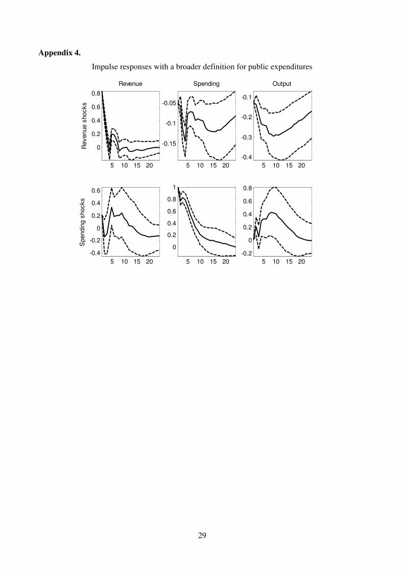
The solid line in Figure 9 is the effect of public expenditures on GDP with public investments
included in the expenditure variable, and the dotted line is the benchmark model response (shown in
Figure 4 before). The figure clearly shows that the response of GDP is clearly greater and somewhat
more persistent with the broader definition for expenditures. In other words, including public
investments in the expenditure variable gives a stronger multiplier effect for public expenditures.
This is at least what this kind of a pure statistical examination gives us.7
4.3. Comparison of VAR and macro model results
In this section, I simulate a similar kind of fiscal shocks with the econometric macro model
(EMMA) developed at the Labour Institute for Economic Research, and compare the results gained
with the results from the structural VAR model. This is done to show how impulse responses may
differ and, also, to produce a kind of robustness test for the benchmark results presented in this
study.
EMMA is a quarterly macroeconomic model which is based on neoclassical synthesis. It is
Keynesian in the short run but its long-run steady state is determined by the supply side of the
economy. It can be classified under the label of “old school” large-scale macro models, even though
its size is relatively small, consisting of 79 equations. The number of behavioural equations in the
7 Impulse responses for all the model variables are shown in Appendix 4.
20
model is 17. The long-run equilibrium relationships and short-term dynamic corrections of the
behavioural equations are estimated using an error correction model (ECM) mechanism. The model
is backward-looking in the sense that is uses historical data.8
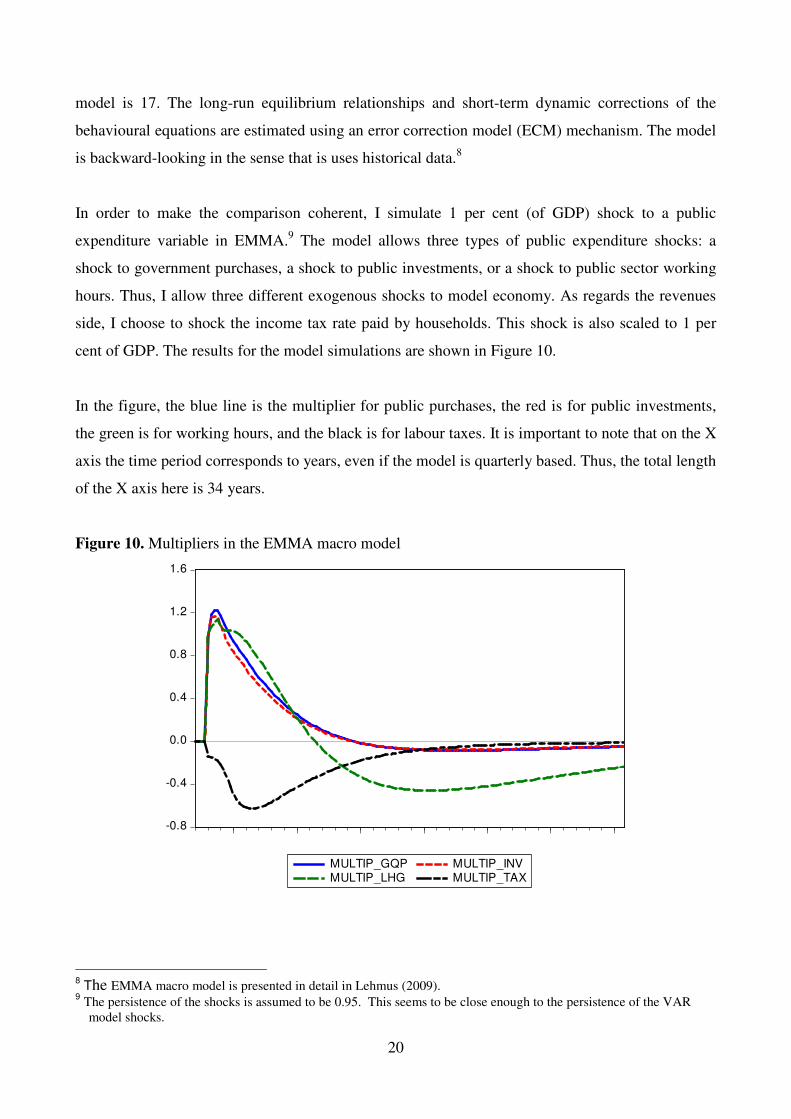
In order to make the comparison coherent, I simulate 1 per cent (of GDP) shock to a public
expenditure variable in EMMA.9 The model allows three types of public expenditure shocks: a
shock to government purchases, a shock to public investments, or a shock to public sector working
hours. Thus, I allow three different exogenous shocks to model economy. As regards the revenues
side, I choose to shock the income tax rate paid by households. This shock is also scaled to 1 per
cent of GDP. The results for the model simulations are shown in Figure 10.
In the figure, the blue line is the multiplier for public purchases, the red is for public investments,
the green is for working hours, and the black is for labour taxes. It is important to note that on the X
axis the time period corresponds to years, even if the model is quarterly based. Thus, the total length
of the X axis here is 34 years.
Figure 10. Multipliers in the EMMA macro model
-0.8
-0.4
0.0
0.4
0.8
1.2
1.6
MULTIP_GQP MULTIP_INVMULTIP_LHG MULTIP_TAX
8 The EMMA macro model is presented in detail in Lehmus (2009).
9 The persistence of the shocks is assumed to be 0.95. This seems to be close enough to the persistence of the VAR
model shocks.

21
The figure shows that in the short run the public expenditure multipliers are bigger than the tax
multiplier and, also, that they are above 1. Nevertheless, the tax multiplier is more persistent in time
than the spending multipliers; the long-run spending multipliers are, in fact, negative.
To compare the results between the VAR and the EMMA macro model, we need to examine the
quarters ranging from 1 to 24 as has been done in all the VAR simulations in this study. Figure 11
draws the results for the expenditure multiplier gained from the benchmark VAR and from the VAR
specification that also includes public investments in the expenditure variable, and on the other
hand the (expenditure) multipliers gained from the EMMA model using the same time span. In the
VAR model specification, I set both parameters 2a and 2b to zero while this is the assumption also
made in the macro model.
Figure 11. Comparison of spending multipliers in VAR and EMMA
0
0,5
1
1,5
2
2,5
1 2 3 4 5 6 7 8 9 10 11 12 13 14 15 16 17 18 19 20 21 22 23 24
Multip_inv_EMMA Multip_gqp_EMMA Multip_lhg_EMMMA
Multip_VAR (spec 1) Multip_VAR (spec inv)

22
Figure 12. Comparison of tax multipliers in VAR and EMMA
-0,7
-0,6
-0,5
-0,4
-0,3
-0,2
-0,1
01 2 3 4 5 6 7 8 9 10 11 12 13 14 15 16 17 18 19 20 21 22 23 24
Multip_tax Multip_VAR (spec 1)
From Figure 11 it can be seen that the expenditure multipliers calculated using the EMMA macro
model are more persistent but smaller in the short run than those gained using the VAR models.
Nevertheless, the differences are moderate both between the VAR and EMMA model multipliers
and also between fiscal policy instruments in EMMA.
The tax multipliers in Figure 12 imply that the VAR model gives a greater tax multiplier in the
short run.(In this case the VAR is only solved using the benchmark model, while public investments
are irrelevant here.) However, the pattern changes in time so that the EMMA model produces a
somewhat stronger tax multiplier in the long run. Hence the time pattern of the GDP response is
somewhat different between the models used in the analysis. In general, the GDP responses of the
macro model seem slightly more sluggish than that of the VAR model, and this applies to both
spending and tax multipliers. The reason for this is probably the Keynesian features of the macro
model which stress the price and wage stickiness of the economy, and which then make the
adjustment of the economy to the shocks slow. Despite this and the fact that the short-run
expenditure multipliers are smaller in EMMA, one can also conclude that the differences between
model-produced multipliers are moderate.
In general, the results are not in contrast with the previous literature. The tax multipliers are
somewhat smaller than, for instance, in Blanchard and Perotti (2002) or Barro and Redlick (2011).
23
However, the results in this paper are similar to B-P and many others in the sense that the tax
multiplier takes more time to build up. The spending multipliers are pretty much in line with the
previous literature; at least they are in the range presented in the summary article by Ramey
(2011b). The bigger estimate for the spending multiplier when public investments are also included
in the expenditure variable is consistent with the views presented in the literature that public
investments enhance the economy’s potential.
Conclusions
Fiscal multipliers have been intensively debated in the economic literature since the onset of the
financial crisis in 2008. Although we now have many research papers on the topic, these papers
mainly deal with the U.S. economy. Nonetheless, the Finnish economy differs from the U.S.
economy with respect to many properties, for instance the exchange rate regime, the share of
exports in output (openness), the size of the public sector, the labour markets, and the industrial
structure. Hence the multipliers from the U.S. studies may not be the best guides when one is
assessing the size of fiscal multipliers for Finland.
To tackle this issue, this study builds a structural VAR model to analyze fiscal multipliers for
Finland. The methods of the study are based on a much cited study by Blanchard and Perotti (2002)
that analyzes fiscal multipliers for the U.S. In this study, I use the Finnish quarterly data for the
period 1975-2011. The data comes from Statistics Finland. The model is based on the
interdependency of three variables: tax revenues collected by the public sector, public consumption,
and GDP. I also analyze the sensitivity of the results to alternative assumptions about the time
dummy controlling the recession in the estimation period and the definition for the public sector
expenditure.
According to two benchmark model specifications, the peak multiplier for public spending gets a
value of 1.30 or 1.56 in the second case. This effect is reached in five quarters after the public
spending shock. However, the effect decreases relatively rapidly and after three years the multiplier
is between 0.59 and 0.81. After that, the multiplier still decreases until it is close to zero. Using the
same specifications, the peak multiplier for an increase in taxes obtains a value of -0.63 or -0.48.
This is reached in nine or seventeen quarters. However, the tax multiplier stays negative for the

24
whole simulation period. Thus, if compared to the spending multiplier, the tax multiplier is smaller
but more persistent in time. When reading these results one should, however, note that confidence
intervals around the produced estimates are quite wide.
Using different time dummies, I get either smaller or greater spending multipliers. Thus, the
spending multipliers are, to some extent, sensitive to the specification of the time dummy. Also,
when public investments are added to the spending variable the model produces a greater spending
multiplier. The tax multiplier is, on the other hand, only slightly affected by the specification
changes. Finally, the comparison of the simulation results between the VAR and EMMA macro
models implies that GDP responses of the macro model are more sluggish than those of VAR(s),
and this applies to both spending and tax multipliers, but the difference between model-produced
multipliers is moderate. Yet the spending multipliers gained from the VAR model are greater than
those from the EMMA model.
References
Almunia, M., Bénétrix, A., Eichengreen, B., O'Rourke, K. H. and Rua, G. (2010): From Great
Depression to Great Credit Crisis: similarities, differences and lessons. Economic Policy, CEPR &
CES & MSH, vol. 25, pages 219-265, 04
Auerbach, A. J. (2012): The Fall and Rise of Keynesian Fiscal Policy. Asian Economic Policy
Review, Japan Center for Economic Research, vol. 7(2), pages 157-175, December.
Auerbach, A. J. & Gorodnichenko, Y. (2012): Measuring the Output Responses to Fiscal Policy.
American Economic Journal: Economic Policy, American Economic Association, vol. 4(2), pages
1-27, May.
Barro, R. J. and Redlick, C. J. (2011): Macroeconomic Effects from Government Purchases and
Taxes," The Quarterly Journal of Economics, vol. 126(1), pages 51-102.
Bernstein, J. and Romer, C. (2009): The Job Impact of the American Recovery and Reinvestment
Plan.
Blanchard, O. and Leigh, D. (2013): Growth Forecast Errors and Fiscal Multipliers. American
Economic Review. American Economic Association, vol. 103(3), pages 117-20, May.

25
Blanchard, O. and Perotti, R. (2002): An empirical characterization of the dynamic effects of
changes in government spending and taxes on output, The Quarterly Journal of Economics, 117(4),
1329-68.
Caggiano, G., Castelnuovo, E., Colombo, V. and Nodari, G. (2014): Estimating Fiscal Multipliers:
News From a Nonlinear World. “MARCO FANNO” Working Paper N.179, University of Padova.
Coenen, G., Erceg, C., Freedman, C., Furceri, D., Kumhof, M., Lalonde, R., Laxton, D., Lindé, J.,
Mourougane, A., Muir, D., Mursula, S., de Resende, C., Roberts. J., Roeger, W., Snudden, S.,
Trabandt, M. and in ’t Veld, J. (2012): Effects of Fiscal Stimulus in Structural Models. American
Economic Journal: Macroeconomics, 4(1), 22-68, 2012.
Delong, J. B. and Summers, L. H. (2012): Fiscal Policy in a Depressed Economy. Brookings Papers
on Economic Activity, vol. 44(1 (Spring), pages 233-297.
Hall, R. (2009): By how much does GDP rise if the government buys more output? Brookings
Papers on Economic Activity, 183-231.
Kuismanen, M. and Kämppi, V. (2010): The effects of fiscal policy on economic activity in
Finland. Economic Modelling, vol. 27, issue 5, 1315-1323
Lehmus, M. (2009): Empirical Macroeconomic Model of the Finnish Economy (EMMA),
Economic Modelling, Volume 26, Issue 5, 926–933.
Owyang, M. T., Ramey, V., and Zubairy, S. (2013): Are Government Spending Multipliers Greater
During Periods of Slack? Evidence from 20th Century Historical Data. American Economic Review,
Papers and Proceedings, May 2013, 103(3).
Ramey, V. (2011a): Identifying government spending shocks: it’s all in the timing. The Quarterly
Journal of Economics 126(1), 1-50.
Ramey, V. (2011b): Can government purchases stimulate the economy? Journal of Economic
Literature 49(3), 673-685.
Riera-Crichton, D., Vegh, C.A., and Vuletin, G. (2014): Fiscal multipliers in recessions and
expansions: Does it matter whether government spending is increasing or decreasing? Paper
presented at JIMF-USC Conference 2014 “Financial Adjustment in the Aftermath of the Global
Crisis 2008-09: A New Global Order?”
Romer, C. and Romer, D. (2010): The macroeconomic effects of tax changes: estimates based on a
new measure of fiscal shocks. American Economic Review 100(3), 763-801.

26
Appendix 1.
0 5 10 15 20 25-0.8
-0.6
-0.4
-0.2
0Tax multiplier
0 5 10 15 20 250
0.5
1
1.5
2Expenditure multiplier

27
Appendix 2.
Impulse responses for dummy for 1991-1993 with 2 0a = , 2 0.21b =
5 10 15 20
0
0.2
0.4
0.6
0.8
Revenue s
hocks
Revenue
5 10 15 20
-0.6
-0.4
-0.2
0
0.2
0.4
Spendin
g s
hocks
5 10 15 20
-0.14
-0.12
-0.1
-0.08
-0.06
-0.04
-0.02
Spending
5 10 15 20
0
0.5
1
5 10 15 20
-0.35
-0.3
-0.25
-0.2
-0.15
-0.1
Output
5 10 15 20
-0.4
-0.2
0
0.2
0.4
0.6
Impulse responses for dummy for 1991-1992 with 2 0.59a = , 2 0b =
5 10 15 20
-0.2
0
0.2
0.4
0.6
0.8
Revenue s
hocks
Revenue
5 10 15 20
-0.6
-0.4
-0.2
0
0.2
0.4
Spendin
g s
hocks
5 10 15 20
-0.2
0
0.2
0.4
Spending
5 10 15 20
0
0.5
1
5 10 15 20-0.5
-0.4
-0.3
-0.2
-0.1
0
Output
5 10 15 20
-0.4
-0.2
0
0.2
0.4
0.6

28
Appendix 3.
Impulse responses for dummy for 1991-1993 and 2009 with 2 0a = , 2 0.21b =
5 10 15 20-0.2
0
0.2
0.4
0.6
0.8
Revenue s
hocks
Revenue
5 10 15 20
-0.4
-0.2
0
0.2
0.4
0.6
0.8
Spendin
g s
hocks
5 10 15 20
-0.15
-0.1
-0.05
0
Spending
5 10 15 20
0
0.2
0.4
0.6
0.8
1
5 10 15 20
-0.4
-0.3
-0.2
-0.1
Output
5 10 15 20
-0.2
0
0.2
0.4
0.6
0.8
Impulse responses for dummy for 1991-1993 and 2009 with 2 0.59a = , 2 0b =
5 10 15 20
-0.2
0
0.2
0.4
0.6
0.8
Revenue s
hocks
Revenue
5 10 15 20-0.5
0
0.5
Spendin
g s
hocks
5 10 15 20
0
0.2
0.4
Spending
5 10 15 20
0
0.2
0.4
0.6
0.8
1
5 10 15 20
-0.3
-0.2
-0.1
0
0.1
0.2
Output
5 10 15 20
-0.2
0
0.2
0.4
0.6
0.8
29
Appendix 4.
Impulse responses with a broader definition for public expenditures
5 10 15 20
0
0.2
0.4
0.6
0.8
Revenue s
hocks
Revenue
5 10 15 20
-0.4
-0.2
0
0.2
0.4
0.6
Spendin
g s
hocks
5 10 15 20
-0.15
-0.1
-0.05
Spending
5 10 15 20
0
0.2
0.4
0.6
0.8
1
5 10 15 20
-0.4
-0.3
-0.2
-0.1
Output
5 10 15 20
-0.2
0
0.2
0.4
0.6
0.8