first assessment of the magnetic-hydrostatic main bearing …
TRANSCRIPT
FIRST ASSESSMENT OF THE MAGNETIC-HYDROSTATIC MAIN
BEARING PROPOSED FOR THE DUCK WAVE-ENERGY CONVERTER
Cohn G Anderson
A Thesis Submitted for the
Degree of Doctor of Philosophy
University of Edinburgh
November 1985
11
ABSTRACT
A preliminary assessment is made of the novel large-scale bearing
proposed for the 'duck wave energy converter. The bearing is
designed to work by combining the principles of self-pressurised
fluid lubrication, and passive permanent magnet repulsion, and
these two topics are dealt with in approximately equal measure.
Following a description of the specification and design of the
bearing, a performance analysis is made, based on standard
lubrication theory assumptions. Although over-simplified, this
predicts favourable characteristics, including high load
capacity, low fluid pressures, and low friction. The analytical
assumptions are then reassessed, and those characteristics of
bearing performance not predicted from lubrication theory, namely
turbulence and fluid inertia, are examined. Both are found to
enhance load capacity, with the most significant effect arising
as an indirect consequence of fluid inertia. The indirect
influence of fluid inertia is described, and experimental
evidence presented of its magnitude, and its asymmetric
characteristic: the experimental model used is that of
converging/diverging radial flow between plane parallel discs.
The permanent magnet repulsion system, and the topic of magnet
geometry optimisation are discussed. After examining the correct
analytical models and optimisation procedures, several
mathematical analyses are detailed. The results of these include
theoretical results for the maximum force, force/unit volume, and
stiffness/unit volume which can be exerted by two-dimensional
rectangular magnets, and the maximum force and force/unit volume
for three-dimensional magnets. Experimental results are included
which verify the theoretical predictions.
The thesis concludes with a short discussion on the overall
feasibility of the proposed bearing.
iii
DECLARATION
Unless otherwise acknowledged, the work, and opinions,
contained in this thesis are my own.
Cohn C Anderson-
Edinburgh Wave Power Project
Department of Mechanical Engineering
University of Edinburgh
November 1985
iv
CONTENTS
Page
Abstract
Declaration
Contents iv
CHAPTER 1 - INTRODUCTION
1.1 Preface 1
1.2 Topics of Study: Chapter Breakdown 1
CHAPTER 2 - LITERATURE REVIEW
2.1 Introduction 6
2.2 Bearing Specification and Design 6
2.3 Performance Analysis 7
2.4 Axisymmetric Radial Fluid Flow 8
2.5 Permanent Magnet Principles 11
2.6 Magnet Geometry Optimisation 12
CHAPTER 3 - THE PROPOSED BEARING: SPECIFICATION AND DESIGN
3.1 Chapter Summary 14
3.2 Wavepower, and the Edinburgh Duck 14
3.3 The Bearing Specification 16
3.4 The Choice of Bearing Mechanism 17
3.5 The Proposed Bearing 22
3.6 Operating Principles 24
3.7 Design Details, and a Precedent 26
3.8 Designing for 25-Year Life 28
3.9 Magnet Axial Alignment 29
3.10 Conclusions 31
CHAPTER 4 - PERFORMANCE ANALYSIS
4.1 Chapter Summary 32
4.2 Analytical Model 32
V
Page
4.3 Stiffness Characteristics (Static Loading) 35
4.4 Damping Characteristics (Dynamic Loading) 35
4.5 Frequency Response 38
4.6 The Two-Dimensional Approximation 42
4.7 Nonlinear Stiffness 42
4.8 The Magnet Sheet 44
4.9 Limitations of Lubrication Theory 44
4.10 Power Dissipation and Temperature Rise 45
4.11 Maximum Pressure, and Pressure Gradient 47
4.12 The Need for Asymmetric Bearing Response 48
4.13 Conclusions 50
CHAPTER 5 - BEARING LUBRICATION IN MORE DETAIL
5.1 Chapter Summary 52
5.2 Flow Regimes 52
5.3 Turbulent Lubrication 54
5.4 Turbulent Power Loss 58
5.5 The Influence of Fluid Inertia 59
5.6 Fluid Inertia: Pressure Drop Across the Magnet Sheet 61
5.7 Convergent Radial Flow 65
5.8 The Importance of the Inertial Pressure Imbalance 66
5.9 The Complete Flow Field 69
5.10 Conclusions 70
CHAPTER 6 - RADIAL FLOW EXPERIMENTS
6.1 Chapter Summary 72
6.2 Experimental Apparatus 72
6.3 Pressure and Flow Measurement 79
6.4 Experimental Results 81
6.5 Quantitative Results Analysis 86
6.6 Conclusions 93
vi
Page
CHAPTER 7 - THE PERMANENT MAGNET REPULSION SYSTEM
7.1 Chapter Summary 94
7.2 Introduction 94
7.3 Magnetic Material Selection 95
7.4 Analytical Models for Permanent Magnets 96
7.5 Optimising the Magnet Geometry 98
7.6 Optimisation Procedures 100
7.7 Related Work 103
7.8 Conclusions 104
CHAPTER 8 - PERMANENT MAGNET OPTIMISATION
8.1 Chapter Summary 106
8.2 Magnetic Forces 106
8.3 Magnetic Stiffness ill
8.4 The Scaling Laws for Force and Stiffness 112
8.5 Geometry Optimisation (1): Constrained Force/Length 114
8.6 Geometry Optimisation (2): .......Stiffness/Length 122
8.7 Optimisation: Applying the Results 127
8.8 Optimisation (3): Unconstrained Force/Volume 129
8.9 Optimisation (4) . .........Stiffness/Volume 133
8.10 Multiple-Pair Magnet Arrangements 137
8.11 Three-Dimensional Optimisation (1): Constrained 142
8.12 Three-Dimensional Optimisation (2): Unconstrained 144
8.13 Conclusions 146
CHAPTER 9 - PERMANENT MAGNET ANALYSIS: EXPERIMENTAL RESULTS
9.1 Chapter Summary 149
9.2 Experimental Objectives 149
9.3 Experimental Apparatus (1): Magnet Levitation-Bed 150
9.4 Experimental Apparatus (2): The Magnets 156
9.5 Verifying the Two-Dimensional Geometry 159
9.6 Force Measurements 163
9.7 Magnetic Stiffness 167
vii
Page
9.8 Demonstration of Non-Uniform Magnetisation 169
9.9 Optimum Geometries Constrained Force/Length 172
9.10 Optimum Geometries .......Stiffness/Length 175
9.11 Optimum Geometries Unconstrained Force/Volume 178
9.12 Optimum Geometries (4) .........Stiffness/Volume 184
9.13 Conclusions 187
CHAPTER 10 - SUMMARY AND CONCLUSIONS
10.1 Performance Characteristics of the Proposed Bearing 188
10.2 The Magnetic Repulsion System 189
10.3 Bearing Feasibility 190
10.4 Suggestions for Further Work 191
References 193
Acknowledgements 201
1
CHAPTER 1
INTRODUCTION
1.1 Preface
The work described in this thesis represents a preliminary
examination of the large scale bearing proposed for the Salter
'duck wave-energy converter.
No prototype of the bearing has yet been constructed. Because
of its dimensions, and the hitherto untried combination of
features which it embodies, it has been considered of paramount
importance first to develop a sound theoretical understanding of
the likely operating characteristics of the bearing. Also,
because the economic viability of the bearing is governed by the
volume of permanent magnet material which is used to provide a
part of its load capacity, optimisation of the magnetic
repulsion system for minimum magnet volume has been identified
as a fundamental requirement.
Following from the above, this thesis concentrates on those
topics judged to be of most importance at this early stage of
the bearing's development. In some cases these are examined to
an extent exceeding that required in the context of the bearing
design. Similarly, certain of the experimental techniques
described may be of interest only in their own right, or in
terms of very different applications to that of the bearing.
In both these respects, it is hoped that this does no more than
reflect the nature of fundamental research.
1.2 Topics of Study: Chapter Breakdown
In chapter 2, a review is made of relevant literature.
Descriptions are included of previous work, although these are
necessarily brief: more detailed aspects of prior research are
included within the appropriate chapters.
2
Chapter 3 begins with a brief description of the duck wave
energy converter, followed by the specification for its main
bearing. Some previous design solutions, and their limitations,
are described. There then follows a description of the
currently proposed bearing design, which operates on the
combined principles of self-pressurised fluid lubrication, and
passive permanent magnet repulsion. The bearing's operating
characteristics are explained, and some details given of its
construction.
In chapter 4, a preliminary analysis is made of the bearing's
operating characteristics. This is based on lubrication theory
assumptions, and a simplified, two-dimensional, analytical
model. The results include mathematical expressions for
stiffness, damping, fluid pressure, load capacity, and power
dissipation; numerical values are then assigned to these
quantities on the basis of provisional bearing dimensions. The
various analytical assumptions are subsequently examined, and
two topics which emerge as worthy of further investigation are turbulent fluid lubrication, and the influence of fluid inertia.
The importance of both lies in their being potentially
load-enhancing.
Chapter 5 contains a more detailed examination of the bearing's
lubrication characteristics, centring on the topics noted above,
ie. turbulent lubrication, and fluid inertia. The likelihood of
the former occurring is estimated on the basis of a film
Reynolds number criterion. An order-of-magnitude estimate of
load capacity is then made assuming turbulent lubrication, and a
Reynolds number-dependent 'equivalent viscosity'. This
calculation, suggested by a previous analysis, is based on a
'turbulent Pois'euille flow' model. The influence of fluid
inertia is then examined, and its importance found to reside in
an 'indirect' effect, which, although fortuitous, may
3
be exploited to significantly enhance the load capacity of the
bearing, and also endow it with a favourably asymmetric
response.
A simplified fluid flow model is proposed to quantify the
indirect effect of fluid inertia: the model is that of
axisymmetric radial flow between plane parallel discs, with the
fluid either diverging from, or converging towards, a central
orifice. The quantity of most interest is identified as the
pressure drop which, in a diverging flow, accompanies the
establishment of a fully-developed velocity profile in the
radial film from initial stagnation conditions upstream of the
orifice. Some previous estimates of this quantity are cited,
and its importance discussed in terms of the performance of the
bearing. Chapter 5 concludes with a brief consideration of the
overall flow pattern in the bearing lubricating film, and a
suggested method for a more detailed analysis.
Chapter 6 is a record of experimental work undertaken to confirm
the appropriate law governing the orifice pressure drop in
axisymmetric, diverging radial flow between plane parallel
discs, and also to make qualitative comparisons between the two
cases of diverging, and converging flow. The influence of
orifice geometry in the former case is also examined, paying
particular respect to the phenomenon of flow separation. The
experimental apparatus is described in some detail, as it
includes certain features thought to be novel, eg. the
hydrostatic load-cell, and hydrostatic calibrated-pressure
source.
Chapter 7 introduces the subject of the permanent-magnet
repulsion system proposed for the bearing, and lists the
criteria for magnetic material selection, detailing the
advantageous properties of 'hard permanent magnets. The topic
of magnet geometry optimisation is raised, where the aim of the
optimisation procedures is to be able to specify any combination

4
of magnet pole-separation and bearing radial force or stiffness,
and then find the minimum quantity of magnetic material required
to achieve it. Emphasis is placed on the important difference
between constrained and unconstrained optimisation procedures;
previous analyses have in general been of the latter kind, which
is not useful in the present application. Both procedures are
nonetheless described, with respect to an isolated,
two-dimensional, symmetric magnet pair: this, for reasons given,
is the appropriate analytical geometry in the present case. The
correct analytical models for hard magnets are then described in
non-mathematical terms.
Chapter 8 contains six theoretical geometry-optimisation
analyses for hard permanent magnets. The two of most importance
with regard to the duck bearing are the area-constrained
optimisations for maximum force and stiffness per unit length of
an isolated, symmetric, two-dimensional magnet-pair. Included
for more academic interest are two unconstrained optimisations
of the same two-dimensional geometry for maximum force and
stiffness/unit volume. The final two analyses deal briefly with
a symmetric, three-dimensional magnet pair, which is optimised
for maximum force, and maximum force/unit volume.
The geometry optimisation schemes differ from those previously
published in several respects. Firstly, they are all based on
rigorous analytical and computer-numerical methods: while prior
analyses have relied on graphical estimates of function maxima,
the present work invokes numerical estimates, found by seeking
the zero values of analytic function derivatives. Secondly,
constrained optimisation analyses of the two geometries noted
above do not appear to have been carried out previously.
Thirdly, the four optimisation schemes dealing with
two-dimensional magnet-pairs - take into account the possibility
of horizontal misalignment of the opposing pole faces: the
situation where the poles are perfectly aligned (previously
considered in some unconstrained optimisations) thus represents

5
a special, rather than the general, case. The results in this
chapter include estimates of the maximum force which can ever be
exerted by a two-dimensional, and also by a three-dimensional,
rectangular magnet pair.
In chapter 9, experiments are described which were carried out
to verify the theoretical results of chapter 8. Only
two-dimensional magnet geometries were investigated, and
magnetic force and stiffness measurements were made using a
specially designed magnetic 'levitation-bed. This is fully
described, and its ability to simulate true two-dimensional
characteristics is illustrated. To interpret, and display, the
experimental results, important use is made of the scaling laws
for magnetic force and stiffness. These are described in
chapter 8, together with the appropriate procedures for
normalisisng results. Chapter 9 also includes a short
discussion of the non-ideal character exhibited by experimental
magnets, with a demonstration of the phenomenon of non-uniform
magnetisation. The possible limitations of ideal-magnet theory
in the context of the overall bearing design are noted.
Chapter 10 is a summary of the thesis, including a discussion of
the overall viability of the proposed bearing, and some
suggestions for further work.
CHAPTER i2
LITERATURE REVIEW
2.1 Introduction
In this chapter, a general review is made of previously
published work. The review is divided into sections, roughly
corresponding to the various topics examined in the thesis.
More specific details of prior analyses, experimental results,
etc. appear in those chapters where context justifies their
inclusion.
2.2 Bearing Specification and Design (Chapter 3)
The current bearing design was first proposed by Salter (1981a)
in a review of the problems facing large-scale wave energy
devices in general, and the duck in particular. The 1985
reference design for the duck is described in UK Department of
Energy publication ETSU R26 (ETSU, 1985a). Of the many wave
energy devices originally proposed in the wake of the oil crisis
of the early nineteen seventies - a good review of them is given
by Shaw (1982) - the duck is one of the few still under active
consideration. The characteristic duck shape was established at
an early stage (Salter, 1974) to maximise energy extraction from
the waves. The current specification for its main bearing is
based on scale tank-tests performed using a model duck mounted
on a rigid axis (Jeffrey et al, 1978), with the maximum
non-reversing load in a calm sea estimated on the basis of tidal
current data for a likely offshore site (Lee, 1981). In
practice, active spine compliance would greatly reduce the
full-scale bearing loads (Salter, 1980) but the fixed-axis force
figures quoted in chapter 3 are nonetheless retained as
conservative design objectives.
Previous bearing design proposals have included a compound
roller-cage/plain bearing (Salter, 1978), and the slubber

7
bearing (Salter, 1980). Although both designs lacked the
essentially contactless load capability of the current proposal,
the slubber bearing exploited wave action to provide a
self-pressurised fluid lubrication capability. This feature has
been retained in the current design (Salter, 1981a) to support
the large reversing wave loads, while a permanent-magnet
repulsion system, acting in parallel, has been proposed to
sustain the much lower non-reversing wave loads. The overall
system is a magnetic-repulsion enhanced, compliant, self-acting,
low pressure hydrostatic bearing. The benefits of compliance in
hydrostatic thrust bearings have been demonstrated by Dowson and
Taylor (1967) and Castelli et al (1967) using high-pressure oil
as the lubricant, and by Levy and Coogan (1968) using
low-pressure air. The closest analogue to the proposed design,
however, appears to be the weeping bearing, which occurs in
nature, in the skeletal joints of large mammals. The mechanism
of weeping lubrication has been proposed, and experimentally
demonstrated, by McCutchen (1959).
Although detailed design is not the purpose of the present work,
certain of the problems facing successful operation of the
bearing are confronted: these include marine fouling, the
proposed solution to which is based on biocidal fouling control
experiments carried out by Picken et al (1981) and invokes the
use of on-board electrolysis of seawater, as recommended by
Hudson et al (1982); the problem of magnet axial misalignment is
likewise addressed, this being threatened by the inherent
instability of passive magnetic repulsion, first predicted in
the classic theorem of Earnshaw (1839).
2.3 Performance Analysis (Chapters 4 and 5)
The simplified lubrication-theory analysis is an adaptation of
that of Archibald (1956) who considered several squeeze-film
problems, among them the dynamic loading of a two-dimensional
full journal bearing, without rotation. Although his analysis
is closely followed, a different integration constant to
Archibalds is assumed when deriving the bearing pressure
distribution; the constant used is that determined by Kuzma
(1970), who derived it from short bearing theory, in the limit
of an L/D ratio tending to infinity.
The general characteristics of bearings operating in a turbulent
lubrication regime have been documented by Constantinescu
(1962), and include increases in both load capacity and
friction, with turbulence identified as a potential advantage in
water-lubricated plastic bearings. A linearised turbulent
lubrication theory was developed by Ng and Pan (1965) based on
the 'law of the wall', in which the derived governing equation
of fluid motion was similar in form to that in the laminar flow
case. The theory is applicable to systems involving shear
(Couette) flow, and was found to account well for prior
experimental results (Smith and Fuller, 1956, Orcutt, 1965) in
terms of both overall load/displacement behaviour, and fluid
pressure distribution. In a subsequent analysis of
thrust-bearing performance under superlaminar conditions,
Wilcock (1977) defined a Reynolds number dependent viscosity,
based on an empirical fit to the theoretical results of Ng and
Pan (above); he then exploited the similarities between the
turbulent and laminar theories, and proceeded to make standard
lubrication-theory (laminar flow) calculations, in which an
effective 'turbulent Viscosity' replaced the usual constant
viscosity term.
2.4 Axisyrnmnetric Radial Fluid Flow (Chapters 5 and 6)
The 'indirect' influence of fluid inertia, which is predicted to
enhance the load capacity of the proposed duck bearing, was
investigated in this study using the model of
diverging/converging axisymmetric radial fluid flow, between
plane parallel discs (see section 1.2). The radial pressure
distribution in such flows was first predicted by Rayleigh
(1917) on the basis of lubrication theory, ie. neglecting fluid
inertia, and assuming viscous, laminar flow. The logarithmic
pressure distribution which he proposed is still universally
used in those cases where inertial effects may be ignored. Of
the earliest attempts to take account of fluid inertia in
axisyminetric laminar radial flows, that of McGinn (1955) is
outstanding: in a comprehensive theoretical and experimental
study, this author proposed the radial pressure distribution to
be a linear combination of Rayleigh's viscous solution, and an
ideal (frictionless) fluid term including a scalar kinetic
energy correction factor, to correct for the parabolic velocity
profile.
More rigorous analyses than McGinns have been made, in general
invoking boundary-layer theory to derive the radial pressure
distribution. Livesey (1959) and Moller (1963) used the
momentum-integral method, Jackson and Symmons (1965a) employed
an iterative method in which inertial effects are treated as a
perturbation to viscous flow, while Peube (1963), Savage (1964),
and Patrat (1975) favoured various methods of series expansion.
Mime (1965) explains the basis of the various methods.
Notably, the resulting expressions for pressure distribution in
the last four of the above analyses reduce, in the first
approximation, to that proposed by McGinn. There seems little
to be gained in the present investigation by preferentially
employing the results of these boundary-layer analyses: none is
strictly valid at small radii (Wilson, 1972), which is the
region of interest in the present study, and none includes entry
conditions appropriate to the situation being modelled. One
further radial-flow investigation worthy of mention is that of
Raal (1978), who performed a sophisticated computer-numerical
analysis. This however dealt with very low Reynolds number
flows, and again employed simplified entry conditions.
Various estimates have been forwarded for the static pressure
drop which corresponds to the establishment of a fully-developed
parabolic velocity profile in diverging, laminar, radial flows
of the kind described above. In a comprehensive review of the

10
effects of inertia in fluid lubrication, Mime (1965) proposed a
pressure correction corresponding to the kinetic energy required
to establish a parabolic profile from initial stagnation
conditions. This assumption was used by Kawashima in his
studies on flat-disc valves (1976, 1978), in which an additional
head loss observed at the film entry was suppressed by
subsequent use of a rounded inlet profile. A slightly lower
estimate (see chapter 5) for the entry pressure drop was
suggested by Mori and Yabe (1966, 1967) in their analyses of
hydrostatic thrust bearings with multiple supply holes. These
authors used a momentum-theory calculation to find the increased
momentum of a parabolic, over a uniform, velocity profile, then
equated the overall pressure loss to the sum of the latter's
momentum contribution plus the calculated increase. A slightly
different technique was used by Vohr (1969), who integrated the
momentum across the width of the parabolic profile (a
boundary-layer technique); this gave a lower value still for the
pressure loss (see chapter 5), although agreement with
experimental data was found to be good.
The phenomenon of flow separation at the entry to a diverging
radial film was experimentally observed, and indeed
photographed, by McGinn (1955). Moller (1963) found that a
rounded inlet profile prevented formation of the separation
'bubble', a similar observation to that of Kawashima (1978).
Vohr (1969) and Jackson and Symmons (1965b) noted a severe
pressure drop immediately downstream of the film entry,
explaining it in terms of flow separation; the latter authors
also suggested that reattachment of the separation 'bubble'
ocurred much further downstream, and was responsible for
asymmetry in the observed radial pressure distribution. The
onset of flow separation was predicted in the theoretical
analyses of Ishizawa (1965, 1966) and Raal (1978), although only
the latter treatment is considered strictly correct, as
Ishizawas analyses invoke an untenable flow-development model
(Wilson, 1972).
11
A turbulent diverging flow will inevitably undergo reverse
transition to laminar conditions once the reduced-Reynolds
number Re (see chapter 6) falls below a certain critical value.
Theoretical predictions of this value range from 10 (Livesey,
1959) down to 4 (Patrat, 1975). The experimental observations
of Chen and Peube (1964) and Kreith (1965) tend to support the
latter figure, with critical Re x values of 4.71 and 4.06,
respectively.
2.5. Permanent Magnet Principles (Chapter 7)
For an overall review of the theoretical principles and
practical applications of permanent magnets, the 1977 text of
McCaig is highly recommended (ref). The same author performed
some of the earliest rigorous experiments using 'hard' permanent
magnets (1961), and consistently advocated the correct
analytical methods to use when dealing with systems comprising
this type of magnet (1968).
The appropriate mathematical models to use in analyses of
all-hard magnet systems (containing no soft iron) are by no
means new, and can be traced to the work of Maxwell (1873). A
hard permanent magnet is commonly treated as either an air-cored
solenoid, or as a pair of pole-faces of uniform charge-density.
The two models yield identical results, and their relative
merits have been compared in a comprehensive review by Craik and
Harrison (1974), with special regard to cylindrically symmetric
magnets. For rectangular magnets (the relevant geometry in this
thesis) the external and internal field strengths can be found
using analytic expressions derived by Craik (1966, 1967) on the
basis of the pole model; these are given in full by McCaig
(1977).
The way in which mutual forces between rectangular magnets may
be calculated is well described by Tsui et al (1972) in a
thorough theoretical and experimental investigation, which
includes a worked example, that of repulsion between two

12
cube-shaped magnets. Solenoid mathematics are used, following
the precedent of Borcherts (1971), and the experimental results
well support the theory, although - importantly - only in cases
where opposing magnets of the same material are used. Full
analytic expressions for the forces of interaction between
two-dimensional rectangular magnets, the geometry appropriate to
many bearing analyses (including the present one), are given by
Yonnet (1980). This author has published a large body of work
on the topic of permanent magnetic bearings, and has pointed out
the important stiffness relationships for these systems (1978a),
which, according to the theorem first proposed by Earnshaw
(1839), must always possess at least one direction of
instability. Yonnets publications include two excellent
reviews of all-permanent magnetic bearings, covering aspects
such as orientation of the magnetic vectors (1978b) and the
advantages of different fundamental bearing configurations
(l98la).
2.6 Magnet Geometry Optimisation (Chapters 8 and 9)
The optimisation procedures in this study all deal with
isolated, symmetric, magnet pairs. Previous analyses of such.
configurations have relied on first deriving an appropriate
objective function such as force/unit volume, or stiffness/unit
volume, plotting this against the magnet dimensions, and hence
finding graphically both the function maximum, and optimum
magnet geometry.
Coffey et al (1972) performed analyses of the kind described
above, to find the maximum force/unit volume available from two-
and three-dimensional rectangular magnet pairs for a given pole
separation. Minnich (1971) performed an essentially similar
analysis of the two-dimensional geometry, recording identical
results (see section 8.8). Cooper et al (1973) examined the
case of a three-dimensional cylindrical magnet pair, finding the
maximum possible force/unit volume, at a given clearance, to
exceed by about 4% that available from rectangular magnets.
13
Yonnet (1981b) optimised the two-dimensional rectangular
geometry for maximum stiffness/unit volume, and also derived an
implicit analytic expression for the magnet pole-width which
maximises stiffness in this configuration, given a specified
pole-height and clearance. All the above optimisation analyses
were unconstrained, in the sense that only pole-separation was
specified, the optimum magnet dimensions then being sought
without prior restriction placed on their ultimate values. The
analyses all assumed full alignment of opposing magnetic poles.
One of the most thorough optimisation schemes to have been
undertaken was that of Henning (1973), who sought to minimise
the volume of track magnet required for a proposed
permanent-magnet levitated ground vehicle. His analysis
employed computer-numerical methods to find the objective
function (in this case force/unit volume) maxima, by seeking the
zero-values of its appropriate first derivative. Although its
solutions were specific to preselected vehicle payload
configurations, the analysis is noteworthy both for its rigorous
mathematical nature, and because it took into account
cross-interactions between the parallel rows of magnets in the
track/vehicle system. Henning's analysis was soundly based on
the prior work of Baran, who first described the basis of the
optimisation procedure used (1971), and reported its preliminary
results in a review (1972).
Indeed, a review of permanent magnet analyses, particularly of
repulsion systems, would be incomplete without mention of Baran,
who may be regarded as a pioneer in the field. On the basis of
the pole-surface magnetic model, this author was perhaps the
first to formulate analytical force expressions for
two-dimensional rectangular magnet pairs (Baran, 1962), and in
subsequent experiments with small permanent magnets, he employed
the elegant technique of using soft iron to simulate closely
spaced opposing pole-faces, thereby finding "satisfactory"
agreement with theoretical force predictions (1964).
14
CHAPTER 3
THE PROPOSED BEARING: SPECIFICATION AND DESIGN
3.1 Chapter Summary
A brief description of the duck wave-energy converter is
followed by the specification for its main bearing.
The limitations of conventional bearing designs in this
application are noted, and two previous design proposals are
described. A description of the currently proposed bearing then
follows, together with an explanation of its operating
principles, in which the distinct roles of fluid lubrication and
passive magnetic repulsion are emphasised. Certain similarities
are pointed out between the fluid lubrication characteristics of
the new bearing and those whiôh exist in a naturally occurring
system. Some design features necessary to ensure a 25-year
operating life in a marine environment are suggested. Finally,
a mechanism is suggested to overcome the problem of magnet axial
instability.
3.2 Wavepower, and the Edinburgh Duck
The duck wave energy converter was originally conceived in
response to the cutback in world oil production of the early
nineteen-seventies, and the current reference design is the
result of a ten-year evolution process. At one time, several
different wavepower devices were under active consideration by
the United Kingdom Department of Energy (see Shaw, 1982), but
current UK policy is unfavourable to their deployment (ETStJ,
1985b). The resource nonetheless remains, and with it the
continuing development of the duck.
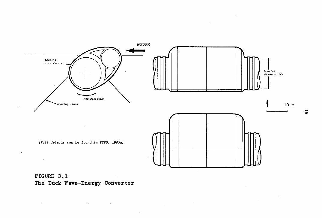
The reference two-gigawatt wave-energy station consists of 896
ducks attached to cylindrical spines, moored in 80-100 metres
water depth, and stationed 35km off the Scottish coast (ETSU,
1985a). Figure 3.1 shows the individual duck/spine unit.
WAVES
(TtflT [hirni bearing diame ter 14m
10
Ln
(Full details can be found in ETSCJ, 1985a)
FIGURE 3.1 The Duck Wave-Energy Converter
The maximum rated output of a single duck is 2.25 MW. Incident
waves cause the duck to rotate, or nod, about its spine, and
by damping this motion, energy is extracted. The
cross-sectional profile of the duck has been developed to
maximise the transfer of energy from the waves, and minimise
the generation of new waves on the leeward side (Salter, 1974).
Although the hydrodynamic principle on which the duck operates
has remained unchanged since its conception, the detailed design
has been subject to continuous development. One feature to have
stimulated considerable thought is the main bearing between the
duck and its spine. The bearing is 37m long with a diameter of
14m, and requires to meet the following specification.
3.3 The Bearing Specification
The target-life for the bearing, in line with that of the
overall device, is 25 years; during this period no significant
degradation of performance should occur.
Wave action imposes unsteady loads, which are comprised of
reversing (cyclic) and non-reversing components. The peak values
of the cyclic loads are estimated as 100 kN per metre of bearing
length at rated output working, and 1000 kN per metre under
freakwave loading. The maximum period for full load reversal
under the conditions of greatest continuous loading is
approximately 7 seconds. The non-reversing component of wave
load under rated output conditions is 10 kN per metre. These
figures are based on scale-model tests of a duck mounted on a
non-compliant axis (Jeffrey et al, 1978), and therefore
represent conservative estimates.
Non-reversing loads, due to tidal currents, can exist even
in the absence of waves. The maximum load, calculated using
data for a typical Hebridean wave-field with current velocity of
approximately 0.5 rn/s (Lee, 1981), is 60 kN per duck (1.6 kN per
metre).
17
Civil, rather than mechanical, engineering tolerances must
be accomodated in the construction of the bearing. Furthermore,
under the stresses imposed by wave loading the spine will bend,
and remain neither truly straight nor round.
A low friction bearing is required. Bearing friction will
squander incident wave-energy, and reduce the efficiency of the
duck. In sea conditions where maximum energy capture is
required, the fractional loss of power can be taken as
approximately twice the bearings coefficient of friction
(Salter, 1981a). Friction also causes wear (see requirement
no.1).
The bearing must operate in a marine environment, with its
attendant hazards of corrosion, and marine-growth fouling. The
possibility of excluding seawater from the duck-to-spine
clearance is considered both unrealistic and undesirable.
The bearing mechanism must be radially thin. This is to
allow, for reasons of strength, the greatest possible spine
diameter.
The bearing surface (shear) velocity is cyclic, with a peak
value of 5 rn/s in the highest waves, (Jeffrey et al, 1978); the
bearing must be load-sustaining throughout the cycle, including periods of zero velocity.
3.4 The Choice of Bearing Mechanism
The suitability, and limitations, of conventional bearing
mechanisms in regard to the above specification can best be seen
by examining four of the commonest types, namely plain, rolling
element, fluid lubricated, and magnetic.
Plain bearings rely on solid-to-solid contact between opposing
surfaces. The lowest obtainable coefficients of friction,
typically 0.04 - 0.12, are probably those achieved using PTFE on
HK
one or both bearing surfaces (Rabinowicz, 1968), but even
assuming the lowest figure, a plain bearing would still
dissipate 8% of the duck's incident power (see requirement 5 of
the specification). More seriously, the corresponding wear
would severely limit the bearing's life.
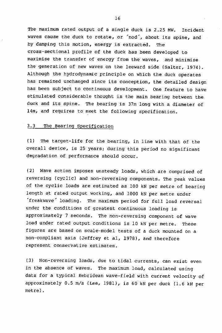
Rolling element bearings can give friction coefficients two
orders of magnitude lower than the best plain designs. At one
stage the roller-cage design shown in figure 3.2 was proposed
(Salter, 1978): the rolling tyres are made of rubber, with the
cage running at half the bearing shear velocity. In heavy sea
conditions, the wave loads cause the tyres to compress, and the
cage to default to behaving as a plain bearing element: in this
way, the power loss is significant only in conditions when power
is abundant. Despite its ability to greatly reduce frictional
losses, the design still required large bearing loads to be
taken by solid-to-solid contact, with the inevitable consequence
of wear. This characteristic ultimately precluded all rolling element designs.
DUCK
0
0 SPINE
plain bearing
0 / surface
FIGURE 3.2 An Early Bearing Proposal (Salter, 1978)
19
Fluid-lubricated bearings offer lower friction still, and
furthermore, the losses in a correctly-operating fluid bearing
do not result in surface wear. Of the three basic types which
can be considered: hydrodynamic, squeeze-film, and hydrostatic,
the first must be discounted. Hydrodynamic bearings can support
no load without relative movement of the opposing surfaces, and
are therefore unsuitable in the present application (see
specification part 8).
In a pure squeeze-film bearing, the load capacity is generated
by surface approach velocity. Although the annular space
between the duck and spine cannot be directly used as a
squeeze-film bearing (which would require too fine, and too
accurate, a clearance), the cyclic loading regime is ideal for
self-pressurised lubrication of a similar kind; this, indeed, is
the basis of the current bearing design (see section 3.5).
In a hydrostatic bearing, coefficients of friction as low as
10 6 can be achieved. Conventionally, such bearings require
high-pressure oil supplies, very fine clearances, and metal
surfaces which have been machined to very fine tolerances. A
bearing of this sort is clearly ill-suited to the duck's
imprecise geometry and harsh working environment. However, the
hydrostatic principle can be applied under very different
conditions. The presence of at least one compliant surface has
been demonstrated to increase load capacity (Dowson and Taylor,
1967, Castelli et al, 1967) and the only constraint on lubricant
pressure is that it be sufficient to support a given load: Levy
and Coogan (1968) have successfully demonstrated a
compliant-surface, hydrostatic thrust-bearing using low-pressure
air as the lubricant.
20
The characteristics of a low-pressure, compliant hydrostatic
bearing, le. the ability to support large loads in an
evenly-distributed fashion, operate with very low friction, and
incur no wear, were at an early stage identified as ideal for
the present application. The original design to exploit them
was the slubber bearing, essentially a self-pressurising,
compliant hydrostatic bearing (Salter, 1980). The slubber
bearing incorporated many of the principles of the present
design, and can be regarded as its immediate predecessor. Its
operating characteristics are explained by referring to figure
3.3.
DUCK
BELLOWS
.. ;••-
0•. • .-....•••.•.•••••-• . ..
............Q ...
• SPINE D • •
'0 • .'• ' 0
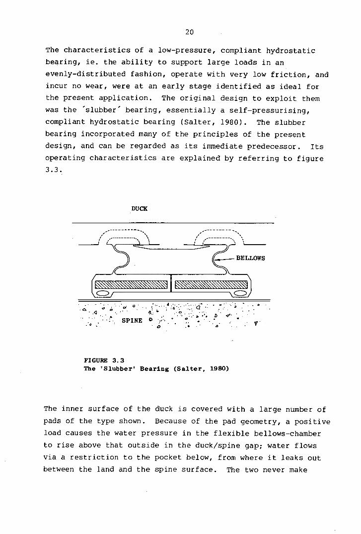
FIGURE 3.3 The 'Slubber' Bearing (Salter, 1980)
The inner surface of the duck is covered with a large number of
pads of the type shown. Because of the pad geometry, a positive
load causes the water pressure in the flexible bellows-chamber
to rise above that outside in the duck/spine gap; water flows
via a restriction to the pocket below, from where it leaks out
between the land and the spine surface. The two never make
21
contact. The pad acts exactly like a circular thrust bearing
when positively loaded, and non-return valves allow its bellows
chamber to recharge during the negative half of the load-cycle.
In this way the slubber bearing exploits to advantage the
seemingly harshest features of its operating environment. The
necessity of a seawater-filled clearance is used to provide the
bearing with a lubricant, while the cyclic nature of the major
wave loads supplies a natural pumping action, operating in
perfect phase with the applied load.
Unfortunately, despite the ideal cyclic-load characteristics of
the proposed slubber bearing, it suffered from the inability to
support non-reversing loads, however small, without some measure
of solid-to-solid contact. The current design overcomes this
problem, by including a parallel load element which is able to
sustain the relatively modest non-reversing loads, using passive
permanent magnet repulsion (see section 3.5).
There are two major types of magnetic bearing, 'active and
passive. Active bearings are deemed unsuitable for the present
application on the grounds of too-high power consumption,
potentially requiring several hundred watts of power per tonne
of load (Salter, 1981a). Passive magnetic bearings employ
permanent magnets arranged either in attraction or repulsion,
and require no power. The maximum load capacity depends on the
magnet material used, and the bearing geometry. Although the
strongest permanent magnets available today can exert maximum
pressures of up to 500 kPa (73 psi), these are little more than
exotic laboratory specimens; the corresponding best which can be
achieved using more conventional magnets is about 36 kPa (5.2
psi). Although this would be insufficient to support large
alternating wave-loads, it is of a suitable order to support the
smaller non-reversing loads. Passive magnetic bearings operate
as contactiess mechanisms, and this feature, allied to their
zero power requirement, makes them ideal in the present context.
22
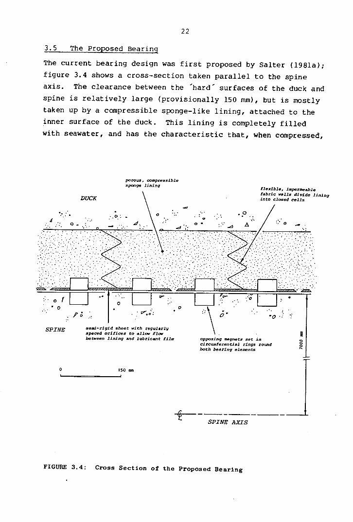
3.5 The Proposed Bearing
The current bearing design was first proposed by Salter (1981a);
figure 3.4 shows a cross-section taken parallel to the spine
axis. The clearance between the 'hard' surfaces of the duck and
spine is relatively large (provisionally 150 mm), but is mostly
taken up by a compressible sponge-like lining, attached to the
inner surface of the duck. This lining is completely filled
with seawater, and has the characteristic that, when compressed,
SPINE semi-rigid sheet with regularly spaced orifices to allow flow
between lining and lubricant film Opposing magnets set in circumferential rings round both bearing elements
0 150=
SPINE AXIS
FIGURE 3.4: Cross Section of the Proposed Bearing
23
it allOws water to be squeezed out only into the narrow
clearance between its base and the surface of the spine. The
function of this narrow clearance is to entrain a lubricating
film. Lateral flow within the lining is prevented by a
combination of its own impedance, and the presence of flexible,
impermeable fabric walls, which effectively divide the lining
into closed rectangular (or other shaped) cells.
The base of the lining is bonded to a semi-rigid sheet with
regularly-spaced orifices in it, these representing the only
route by which water can pass between the lining and the narrow
clearance. Fixed to the sheet are permanent magnets: these take
the form of rectangular blocks laid end-to-end, forming parallel
closed rings round the circumference of the bearing. Opposite
the magnets in the sheet, and oriented in mutual repulsion with
them, are similar rings inlaid in the surface of the spine.
Both the compressible lining and the repelling magnets have
spring characteristics, and when an external force acts to close
down the duck-to-spine hard clearance, the lining thickness and
the magnets pole separation decrease in inverse proportion to
their relative stiffnesses.
Assuming lateral fluid pressure gradients to be small, it is the
ratio of magnetic to lining stiffness which alone dictates the
dimensions of the thin lubricating film. The magnetic stiffness
is much the greater, provisionally by up to 50 times, so that a
force which causes a large lining compression gives rise to a
much smaller decrease in pole clearance. In this way, the
lubricating film can potentially be maintained despite large
relative excursions of the duck and spine. Although the film
equilibrium thickness, provisionally 2-3 mm, is very large by
normal lubrication standards, the ratio of film thickness to
flow path-length is of the order of lO g , similar to that of a
small scale squeeze-film bearing.
24
3.6 Operating Principles
Consider now, the effect of a wave load acting on the duck, and
tending to close down the bearing 'hard clearance. As the two
hard surfaces approach, the compliant lining compresses, causing
water to be squeezed out of the lining into the
narrow-clearance, where it is then free to flow axially to the
ends of the bearing, or circumferentially round to the other
side, according to the local pressure gradients. Flexible
impedances incorporated at the extreme ends of the bearing can
be used to encourage flow preferentially round its
circumference. No lateral flow of water takes place within the
flexible lining, which discharges the water it contains via the
orifices in the magnet-sheet, into the lubricating film: the
sheet effectively behaves as a compliant hydrostatic thrust pad
with multiple supply holes.
With a favourably high film thickness ratio (ie. an escape path
several thousand times the thickness), significant increases in
fluid pressure, and hence load capacity, can potentially be
sustained. However, the bearing dimensions should ensure that
the fluid pressures and pressure gradients will, in absolute
terms, be very low. The pressure gradient across the width of
the hard clearance will largely be that associated with the
orifice discharge of water from the lining, and to a first
approximation, the film thickness will be independent of local
water pressure (it is explained in section 5.5 how the orifice
pressure drop should actually enhance load capacity). The
duration for which the bearing can sustain a wave load will be
determined by the time it takes to completely discharge the
lining, and is potentially many times greater than the reversal
time of the longest wave-loads.
While the squeezing action on the loaded side of the bearing
discharges water from the lining, the lining on the other side
recharges. This not only results in the bearing being ideally
suited to a cyclic load regime, but also has the important

25
consequence that both loaded and 'unloaded' sides of the
bearing contribute to the overall load capacity (and should
strictly be referred to as positively and negatively loaded).
The recharging lining draws water back through a clearance
almost as narrow as that on the positively loaded side, and a
negative pressure gradient will therefore exist in the lubricant
film, corresponding to a positive contribution to the overall
load-capacity. The net effect is an even spreading of the load
round the entire bearing circumference.
In this way, the large cyclic loads are resisted by hydrostatic
pressure, self-generated in the bearing. The non-reversing
loads can create no such pressure, and are instead supported by
permanent-magnet repulsion. The magnet arrangement is
essentially that of a stacked multi-element radial bearing,
where each element consists of two concentric rings of
rectangular section (the inner ring being that on the spine
surface). Precompression of the compliant lining during bearing
assembly is proposed to establish the equilibrium magnetic pole
clearance.
The magnets and compliant-lining represent a pair of springs
connected in series; the relative displacement of duck to spine
under a non-reversing load will therefore be dictated by the
weaker spring, ie. the lining. The essential lubricating film
thickness should be maintained despite significant
non-uniformities in the spine geometry: the semi-rigid sheet in
which the magnets are mounted is designed to be rigid locally,
but with sufficient compliance to conform to large-scale
deviations of the spine surface, and this characteristic ought
to be enhanced by a high value of magnetic repulsion stiffness.
The key features of the proposed design are an ability to
withstand low non-reversing loads indefinitely, and large
alternating loads for periods greatly in excess of those which
ever occur in practice, in both cases without the load-carrying
26
surfaces ever touching: the bearing has thus been designed for
zero wear. This does not imply zero friction, but means that
any frictional energy losses will take place entirely within the
lubricating water.
3.7 Design Details, and a Precedent
The same pressure gradients which dictate the flow in the
lubricating film also exist, in the compliant lining directly
above it. Because the pressure gradients will be low, however,
the lining need have only modest resistance to lateral fluid
flow. A natural or synthetic foam rubber is the most probable
material for the lining; the flexible cell walls can be made
from fabric-reinforced rubber. For the semi-rigid sheet in
which the magnets are embedded, a material is required which has
the characteristics of thin plywood, or glass-reinforced
plastic. One suggestion is for a rubber sheet stiffened with
wire mesh (Salter, 1981a). The nature of the magnets themselves
is discussed in greater detail in chapter 7, but it can briefly
be noted that the magnetic blocks will be made of anisotropic
barium or, strontium ferrite, which materials combine the
favourable properties of good magnetic strength and stability in
repulsion applications, total resistance to corrosion, and
relatively low cost.
The proposed design has been called a 'magnetically enhanced
squeeze-film bearing', but this is a misnomer. In a true
squeeze-film bearing, the fluid-flow in which the load-capacity
is developed is bounded by two converging bearing surfaces; in
the duck bearing, the lubricating film-width stays approximately
constant during a load cycle, with relative movement of the two
surfaces contributing very little to load pressure. A strict
description of the bearing would be 'magnetic-repulsion
enhanced, self-pressurising, compliant-hydrostatic'. Although
this combination of features is perhaps novel, it may be
observed that the design actually comprises a parallel
arrangement of two well-established components. The first of
27
these is a passive permanent-magnet repulsion bearing. The
second has been called a weeping, or'sponge-hydrostatic',
bearing, and exists in nature, in the articular joints of
various species of large land mammal.
The mechanism of weeping lubrication was first proposed by
McCutchen (1959) to explain the ability of skeletal joints to
support very high loads - up to one ton per square inch - with
minimal friction, notably in cases where the relative velocity
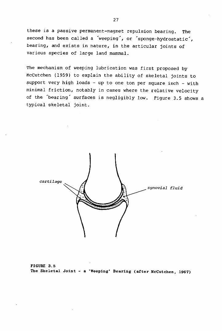
of the bearing surfaces is negligibly low. Figure 3.5 shows a
typical skeletal joint.
cartilage
synovial fluid
FIGURE 3.5 The Skeletal Joint - a 'Weeping' Bearing (after McCutchen, 1967)

The opposing surfaces are each covered with a layer of articular
cartilage, resembling a microporous sponge, which is filled with
a liquid lubricant (the synovial fluid). An applied load causes
the cartilage to compress, and weep fluid into a tiny
clearance between the surfaces, from where it has a long
escape-path to the edges of the joint. Fluid pressure thus
builds up sufficient to support the load; the cartilage acts in
parallel, but only experiences the small compression force
dictated by its own stiffness. For the joint to operate in this
manner, the cartilage characteristics must be very similar to
those of the proposed lining for the duck bearing: indeed, in
one experimental simulation, McCutchen used a layer of
closed-cell sponge with pinhole perforations in it to direct the
flow - an arrangement very similar to that shown in figure 3.4.
His experiments proved the mechanism to work, but highlighted
that a positive load capacity can only be sustained for a finite
time, after which the compressed surfaces have to recharge with
fluid.
The articular joint is not a perfect analogue of the duck
bearing, however, as it does not rely entirely on weeping
lubrication (McCutchen, 1967; Dowson, 1967) and some degree of
surface-to-surface contact occurs. In the duck bearing, natural
running repairs will not be possible, and for this reason the
permanent-magnet system is included to ensure zero surface
contact. Nonetheless, the operating principle of the weeping
bearing is obviously sound, and it can be argued that it has
been more thoroughly developed and tested than that of any
other.
3.8 Designing for 25-Year Life
Two major threats to the specified design life of the bearing
are corrosion, and marine fouling - the disadvantages of an open
bearing which uses seawater as a lubricant. To prevent
corrosion, non-metals will be used almost exclusively in
construction, eg., plastics, natural and synthetic rubber, and
29
glass-reinforced plastic. Ferrite magnets do not corrode by
virtue of their chemical composition, which is very similar to
that of the iron oxide in rust.
To prevent marine fouling, and in particular the potential
growth of hard-shelled species on the bearing surfaces,
treatment of the bearing water with a biocide is proposed.
Although dependent on the level of wave action, the time taken
for complete exchange of the water in the bearing will be long
(provisionally 24 hours), thus maximising the efficiency of any
toxic agent released into the clearance. One of the most
effective methods of fouling prevention is continuous low-level
chlorination. The concentration of this toxin is of less
importance than the length of time for which it is administered
(Picken, 1981), and the presence of 0.02 -.0.05 ppm of chlorine
continuously active in the bearing would be enough to deter the
settlement and growth of hard fouling species which could resist
much higher intermittent doses of the biocide. Chlorine
generation by on-board electrolysis of seawater is possible, and
has been recommended as particularly suitable for wave-energy
converters, due to the ready availability of electricity, the
absence of ecological side-effects, and the safety of
installation and operation (Hudson et al, 1982).
3.9 Magnet Axial Alignment
The bearing has so far been described as a pure non-contact
design. There is, however, a fundamental reason why this can
never be entirely true in practice, and that is the inherent
instability of passive magnetic repulsion. This instability
applies equally to attractive systems, and was first identified
by Samuel Earnshaw in his classic theorem of 1839 (ref). The
theory shows that completely free levitation using passive
permanent magnets can never be stably achieved, and that there
must always exist at least one direction in which movement will
be unstable. For the magnets in the bearing, this direction is
parallel to the spine axis. In another form, Earnshaws theorem
30
shows that for a bearing of this kind, the stiffer the magnetic
repulsion is radially, the greater will be the axial instability
(see section 8.3).
It is therefore necessary to provide some mechanical means to
restrict the relative axial movement of the magnetic rings, and
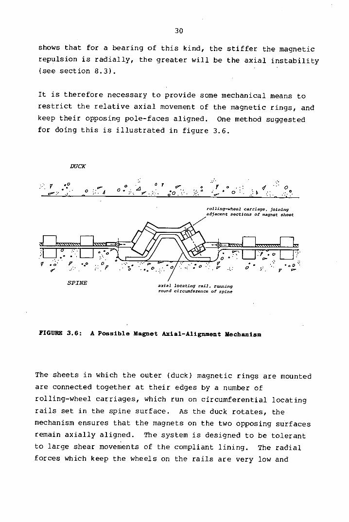
keep their opposing pole-faces aligned. One method suggested
for doing this is illustrated in figure 3.6.
DUCK
•.:.y •!' o °T •41
. o o .:
o 0..: ..• • .: . :
- .... I.' .. '•:.•• oO. .:. .: .:
rolling-wheel carriage, joining adjacent sections of magnet sheet
•
0:0
V . o • P .o o •.• p •. ,
SPINE axial locating rail, running
round circumference of spine
FIGURE 3.6: A Possible Magnet Axial-Alignment Mechanism
The sheets in which the outer (duck) magnetic rings are mounted
are connected together at their edges by a number of
rolling-wheel carriages, which run on circumferential locating
rails set in the spine surface. As the duck rotates, the
mechanism ensures that the magnets on the two opposing surfaces
remain axially aligned. The system is designed to be tolerant
to large shear movements of the compliant lining. The radial
forces which keep the wheels on the rails are very low and
31
practically constant, being dependent only on the lining
stiffness, and not the fluid pressure. With the magnets in
perfect alignment, the axial forces are theoretically zero, and
so the nearer this condition can be met, the less will be the
wear of the rolling wheels. The angled section of the rails
shown in figure 3.6 is designed to ensure that, assuming equal
wear of the wheels on either side, no misalignment will result.
3.10 Conclusions
The bearing specification has been detailed, on the basis of
scale-model experiments. To meet the specification, the current
bearing proposal combines .the principles of self-pressurising,
compliant, hydrostatic lubrication, and permanent-magnet
repulsion. The bearing uses treated seawater as its lubricant,
and exploits the large scale of the duck in its operation, with
a lubricating film thickness ratio comparable to that of a small
scale squeeze-film bearing. The large cyclic loads imposed by
wave action will be supported almost entirely by fluid pressure,
and the lower non-reversing loads by magnetic repulsion. The
design is contactless, save for the necessary magnet axial
alignment mechanism: this, however, is subject to only small and
uniform loads. Load distribution over the bearing area will be
even, with fluid pressures and pressure gradients low as a
result. To ensure its longevity, the bearing will be
constructed from non-corroding materials, and the seawater
lubricant will be electro-chlorinated to prevent fouling.
32
CHAPTER 4
PERFORMANCE ANALYSIS
4.1 Chapter Summary
In this chapter, a preliminary analysis is made of the bearing's
performance characteristics. Both static and dynamic loading
are considered, in the latter case using a simplified
two-dimensional model and 'classical' lubrication theory
assumptions. The results include expressions for bearing
stiffness and damping which are subsequently incorporated in an
equation of motion, in order to estimate the bearings response
to cyclic loading. On the basis of provisional bearing
dimensions, performance characteristics are calculated including
maximum eccentricity, maximum power dissipation, temperature
rise, friction coefficient, and maximum fluid pressure. The
assumptions made in the analysis are examined, and the
desirability of an asymmetric response to cyclic loading is
explained.
4.2 Analytical Model
In order to make useful predictions of the bearing's performance
characteristics without invoking a prematurely high level of
mathematics, a simplified model of the system is proposed. With
reference to figure 4.1, the following assumptions are made:
The bearing is assumed to be two-dimensional, with all
fluid flow taking place in the plane of figure 4.1. End leakage
is therefore neglected.
The compliant lining is represented as a porous, isoelastic
layer attached to the inner surface of the duck, and occupying
most of the duck-to-spine hard clearance. The lining is
absorbent, in the manner of a sponge, but possesses anisotropic
flow characteristics. Water can flow only radially in or out of
it, according to whether it is being recharged or discharged,

33
inner 'hard surface of duck . ... : • •:.:. ::::
spine surface Ap
equilibrium axis
displaced axis )J.. PROPORTIONS NOT TO SCALE
compressible, porous . . . . :•. . ..::
lining . ••.• . .. ...
lubricating film (equivalent to magnetic pole clearance)
NOTATION (provisional dimensions in brackets)
b bearing axial length (37m)
e displacement
h narrow clearance
he is at equilibrium (3mm)
H gross clearance
He at equilibrium (0.15m)
r spine radius (7m)
W applied load
Mli
NON-DIMENSIONAL PARAMETERS
E eccentricity = e/He
m gross clearance ratio He/r (0.021)
A lining thickness ratio = h/H (0.020)
FIGURE 4.1 Bearing Cross Section: Diagrammatic
34
respectively, and no lateral flow takes place within it. In
this way, a given section of the lining can communicate water
only into or out of the narrow clearance bounded by its base,
and the surface of the spine. No losses are assumed in the flow
in or out of the lining, and hence, pressure gradients across
the hard clearance are neglected, with the pressure in the
lubricating film taken to be the same as that in the adjacent
lining.
The semi-rigid sheet which forms an inner skin to the
lining, and on which the duck magnets are fixed, is ignored.
Although water flows in and out of the lining only through the
orifices in this sheet, these are disregarded, and flow across
the lining inner surface is assumed to occur uniformly over its
area. The magnetic rings are not considered as rigid elements;
bending and shear forces in the magnet sheet are neglected, and
its mass and thickness are also disregarded.
The radial stiffnesses of both the lining and the repulsion
magnet system are taken to be constant. Both elements could be
mechanically represented by annular nests of radially-directed
springs. In the case of the lining, both axial and
circumferential strain are neglected. Similar assumptions have
been made in analyses of compliant-surface thrust bearings with
elastomeric surfaces (see Castelli et al, 1969): in the present
case, however, the compliant lining is both compressible and
porous, unlike an elastomer.
Classical lubrication theory assumptions are made: flow
in the lubricating film is assumed to be viscous-dominated and
laminar, with fluid inertia neglected.
In due course several of the above assumptions, not least those
pertaining to lubrication theory, are placed under scrutiny.
35
4.3 Stiffness Characteristics (Static Loading)
Under a static displacement e from equilibrium, the gross
(hard-surface) bearing clearance H is given approximately by:
H = He e cos O (4.1)
The compliant lining thickness is approximately equal to the
entire gross clearance. Hence if the lining compressibility
constant, with units of pressure per unit radial deflection, is k5 , then the local spring pressure P s exerted on the inside of the duck at angle 0 to the load-line is found from:
PS = P 5 (equiln.) + k 5 e cosO (4.2)
The applied static load WS is resisted by this pressure according to:
ws = 2f P 5br cosO dO (4.3)
And hence, using the non-dimensional notation given in figure
4.1,
WS = k5b7imr2E (44)
Thus the static deflection obeys a linear spring law. The
lining compressibility constant k 5 would be chosen to match a dsired maximum static eccentricity E to a particular static
load W5 . The other terms in equation 4.4 are determined by the bearing dimensions.
4.4 Damping Characteristics (Dynamic Loading)
The following analysis is an adaptation of that of Archibald
(1956), who considered the case of a two-dimensional
full-journal bearing, subject to dynamic loading, but without
rotation (one of a number of squeeze-film analyses carried out
by this author). In his analysis, Archibald first derived an

36
expression for the circumferential pressure gradient in a
dynamically loaded journal, by equating two expressions for
lubricant flowrate. One of these was based on geometric
considerations, and the other on the lubrication-theory
expression for the one-dimensional flow of a viscous fluid
between plane parallel walls (see eg. Barwell, 1979).
Expressions for pressure distribution and load were subsequently
found by integration. In the present case, Archibald's analysis
is adapted to take account of the compliant lining in the duck
bearing (whose simplified properties are noted above).
Consider a constant load Wd acting on the outer bearing element,
causing time-dependent displacement e and velocity 6 . At an angle e to the load-line, the volume flowrate through the narrow clearance h is found from geometric considerations by:
q = br sinO de/dt (displacement flow) (4.5)
in which all the fluid squeezed out of the compliant lining is
assumed to flow through the narrow clearance maintained by
magnetic repulsion. From lubrication theory, the flowrate is
also given by:
-bh 3 q =2r
dP/d® (viscous flow) (4.6)
Equating these gives the circumferential pressure gradient:
-12jir 2 sinO
dP/dO = de/dt (4.7) h 3
Assuming negligible pressure gradients across the gross
clearance, the narrow clearance h is determined only by the
balance of spring forces on the two sides of the magnet sheet.
If these are selected to obey a linear relationship, with:
h = XII (4.8)

37
then the pressure gradient is given by:
-12j.t sine dE/dt
m' A' (1 - E COS O)3 (4.9)
in which non-dimensional notation is again used (see figure
4.1). The pressure distribution round the circumference is
found by integrating equation 4.9, hence:
P(e) = 6dE/dt 1
+ c } ( 4.10) m2 A 3 E (1 - Ecos0) 2
in which C is a constant of integration, whose value is taken
as that determined by Kuzma (1970) for a two-dimensional full
journal bearing, ie.:
C. = 1
(2 +3E 2 )
(Kuzma, 1970) (4.11)
In Kuzmas analysis, the constant is derived from short-bearing
theory, in the limit of an L/D ratio tending to infinity; the
author explains why only this approach is strictly correct. The
value of C does not however influence total dynamic load Wd,
which is found by integrating incremental pressure loading round
the bearing circumference (cf. equation 4.3). Doing this in the
present case, the load is found from:
12irpbr dE/dt = (4.12)
in 2 A 3 (1 - E 2 ) '2
The above result invites comparison with the two cases of:
A conventional journal bearing of the same length and
diameter, and clearance equal to the present gross clearance H.
A journal bearing of again the same dimensions, but
clearance equal to the narrow (lubricating film) clearance h.
In the first of these, the load is found from equation 4.12
using A = 1, with the resultant load value then A 3 times that

W.
for the proposed bearing. In the second case, the load will be
A times that of the new bearing. The constant X, which
represents the lubricating film thickness to gross clearance
ratio, is provisionally 0.02: the proposed design is thus
predicted to have 125,000 times the load capacity of a similarly
sized journal-bearing, and, perhaps surprisingly, 50 times the
load capacity of a bearing with one-fiftieth the hard-surface
clearance. To explain the latter finding, the new design could
be compared to a journal bearing with narrow clearance h, and a
replenishable lubricant supply which increased its
load-supporting time by a factor of 1/A.
4.5 Frequency Response
Consider, now, the outer bearing element to be subject to a
unidirectional alternating load F 0sinwt, representing the
component of wave load causing relative movement of the duck and
its spine (as opposed to simultaneous acceleration of both
components). If the effective mass of the duck, including added
hydrodynamic inertia terms, is M, then the equation for the
relative motion will be:
M d2 e/dt 2 = F0 sin wt - bearing forces (4.13)
The bearing forces are given by equations 4.4 and 4.12, and
hence:
ME + CE + KE = (F 0 /mr) sin wt (4.14)
where:
l2irjtb C
M3 A 3 (1 - E 2 ) 3/2
K = k5bur
39
It can be seen that the damping coefficient C is nonlinear,
increasing with eccentricity E - however, if E is small, then:
127rjtb C = (4.15)
M3 A3
and under these conditions the equation of motion may be treated
as linear. If the provisional dimensions given in figure 4.1
are now used to assign numerical values to the above
coefficients, and assuming a lining compressibility constant k 5 of 9190 N/m2 per metre deflection, the following values are found:
C = 1.77 x 10¹⁰ kgs
K = 7.48 x 10⁶ kgs 2 (4.16)
Because of its added inertia, the ducks effective mass N is
dependent on wave-frequency, but will be of the same order as
the 'dry' mass of 3400 tonnes (3.4 x 10 6 kg). Using these
figures it may be seen that damping very strongly dominates the
equation of relative motion (equation 4.14), with a ratio of
actual to critical damping in excess of 1000. Forced resonance
poses no apparent threat to the bearing. The dimensionless
response of the bearing to the forcing function can then be
found from the approximate formula:
E = Emax Sjfl ( 27rft - ir/2 ) (4.17)
where:
F 0 Emax - _______
2yrfmrC
40
The maximum hard-surface approach velocity is given in
dimensional, and non-dimensional, forms respectively by:
F 0 emax = (4.18)
C
F 0 Emax = (4.19)
mrC
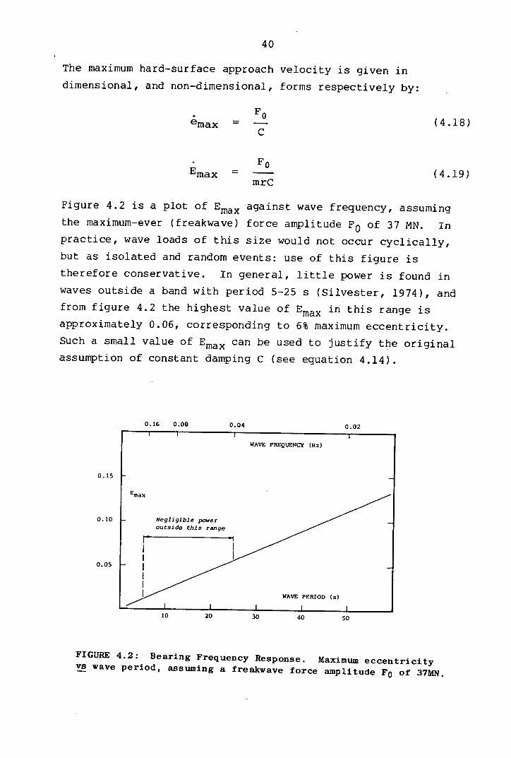
Figure 4.2 is a plot of Emax against wave frequency, assuming
the maximum-ever (freakwave) force amplitude F 0 of 37 MN. In practice, wave loads of this size would not occur cyclically,
but as isolated and random events: use of this figure is
therefore conservative. In general, little power is found in
waves outside a band with period 5-25 s (Silvester, 1974), and
from figure 4.2 the highest value of Emax in this range is approximately 0.06, corresponding to 6% maximum eccentricity.
Such a small value of Emax can be used to justify the original
assumption of constant damping C (see equation 4.14).
nt; n (Q - --
0.15
0.10
0.05
30 40 50
FIGURE 4.2: Bearing Frequency Response. Maximum eccentricity vs wave period, assuming a freakwave force amplitude F0 of 37MN.

41
The response of the bearing to real, irregular wave loads can be
investigated on the basis of the linearised equation of motion,
and experimental wave force records. Figure 4.3 shows
time-records of the two orthogonal components of wave force in a
typical 'mixed sea.
MODEL SCALE: 1/140
force (MN)
+4 T horizontal (surge)
-4 i
T vertical (heave)
-4 i
I ...__. .1. ._.. ...I._.., .. ,._.,....I..._,...... .1 I
0 50 tOO 150 200 250 time (s)
RESULTS SCALED UP FOR 37m DUCK
FIGURE 4.3: Experimental Wave Force Records
The measurements are scaled up from model test results. The
bearing response to these may be predicted either by first using
a Fourier analysis to convert the force records to a set of
component frequencies, and then summing the individual responses
to these, or more directly by examining an integrated force
record, the instantaneous value of which is approximately
proportional to bearing displacement. Although neither analysis
is included here, the bearing response is predicted to be safe
due to the continually reversing nature of the loads shown in
figure 4.3, and the comparatively small magnitude of the
non-reversing components (see section 3.3).
On the basis of the analysis so far, the operating
characteristics of the bearing are predicted to be favourable.
It is therefore important to now examine in more detail some of
the assumptions underlying the simplified analytical model.

42
4.6 The Two-Dimensional Approximation
For plain journal bearings, the assumption of no axial flow is
usually deemed reasonable for L/D (length/diameter) ratios
greater than about four (see eg. Massey, 1979). Although the
duck bearing has an L/D ratio of 2.64, it can incorporate
flexible impedances at its ends to minimise axial leakage and
increase its 'effective L/D ratio'. However, even assuming end
leakage to halve the minimum damping coefficient C, the result
would still be only 12% maximum eccentricity under freakwave
loading.
Skew loading must also be considered. Because incident waves
are not in. general parallel to the bearing axis, phase
differences will exist between the forces experienced along its
length. The instantaneous difference in the force exerted at
the two ends of the bearing can be roughly estimated using
theoretical correlation coefficients for multidirectional wave
spectra (Salter, 1981b): these reflect the similarity of the
instantaneous forces at different distances along the length of
the duck. Assuming the most severe conditions, the difference
in force is predicted to be about 30% of the mean value. The
precise effects of skew loading require more detailed analysis,
but no catastrophic implications seem obvious at this stage.
4.7 Nonlinear Stiffness
So far, constant stiffness has been assumed in both the
compliant lining and the repulsion magnet system. In practice,
however, magnetic stiffness increases strongly with decreasing
pole separation (see section 8.3). A comparison of the
relationships between narrow and gross clearances (h and H
respectively) for the two cases of constant and nonlinear
magnetic stiffness is seen in figure 4.4. The nonlinearity
depicted is arbitrary, but chosen to represent a case where the
equilibrium film thickness he is the same in the two cases.
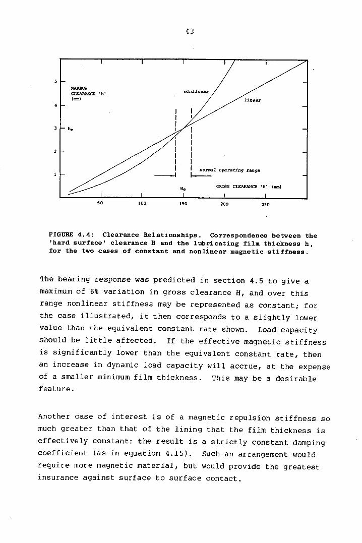
43
5
4
3
2
1
NARROW nonlinear
CLEARANCE h' / (mm) linear
he
I normal operating range
He GROSS CLEARANCE H (mm)
I I I I 50 100 150 200 250
FIGURE 4.4: Clearance Relationships. Correspondence between the 'hard surface' clearance H and the lubricating film thickness h, for the two cases of constant and nonlinear magnetic stiffness.
The bearing response was predicted in section 4.5 to give a
maximum of 6% variation in gross clearance H, and over this
range nonlinear stiffness may be represented as constant; for
the case illustrated, it then corresponds to a slightly lower
value than the equivalent constant rate shown. Load capacity
should be little affected. If the effective magnetic stiffness
is significantly lower than the equivalent constant rate, then
an increase in dynamic load capacity will accrue, at the expense
of a smaller minimum film thickness. This may be a desirable
feature.
Another case of interest is of a magnetic repulsion stiffness so
much greater than that of the lining that the film thickness is
effectively constant: the result is a strictly constant damping
coefficient (as in equation 4.15). Such an arrangement would
require more magnetic material, but would provide the greatest
insurance against surface to surface contact.

44
4.8 The Magnet Sheet
Bending moments and shear forces in the compliant magnet sheet
have been neglected. In operation, the deviation of the sheet
from its equilibrium annular shape will correspond to a diameter
variation of no more than 0.05%. Allied to the required
compliance of the material, this appears to justify the initial
assumption. Similarly, the mass, and hence inertia, of the
sheet are neglected on the grounds that its radial velocity and
acceleration are insignificant. Its physical dimensions can be
incorporated into the definition of the gross clearance H, and
do not affect the analysis.
4.9 Limitations of Lubrication Theory
The lubrication-theory assumptions detailed in section 4.2
require to be revised. In particular, the possibility of
turbulence in the lubricating film, and the influence of fluid
inertia, cannot be ignored. These important topics are further
investigated starting in the next chapter.
The assumption of negligible pressure drop across the bearing
hard clearance is not correct. A difference in pressure will
exist across the magnet-sheet orifices where the compliant
lining is discharging water into the narrow clearance, and any
section of the sheet through which water is being squeezed will
therefore experience net fluid loading. This loading will tend
to reduce the magnets clearance until the accompanying increase
in repulsion cancels it out: the lubricant film thickness is
therefore not determined solely by the balance of magnetic and
lining stiffnesses, but also by the local fluid flow
characteristics. The implications of this are important, as a
potentially greater load capacity can accrue. This topic is
further discussed in chapter 5.
45
4.10 Power Dissipation and Temperature Rise
The bearing dissipates power as heat due to viscous damping of
(a) the relative radial motion of duck and spine, and (b) the
duck's angular (nod) rotation. Only rotation damping will
result in loss of useful power from the duck, but both effects
contribute to raising the temperature of the bearing water.
The power dissipated in the first case can be calculated as the
product of load and approach velocity, thus:
Maximum Power Dissipation Pmax = Foémax (4.20)
where 6max can be substituted using equation 4.18, giving:
F 2 Maximum Power = (4.21)
C
The damping coefficient C was provisionally evaluated in
equation 4.16. The appropriate value of F0 in this case is the load at maximum rated output, rather than the maximum isolated
(freakwave) load which must be withstood, hence for a 37 metre bearing, F0 = 3.7 MN (see section 3.3), giving:
Maximum Power = 800 watts (4.22)
The damping of the ducks rotation is calculated as a shear
loss, from:
jiAv 2 shear =
h
(4.23)
where the bearing surface area A = 1627 m 2 , the limiting rms surface velocity v = 0.61 rn/s (Jeffrey et al, 1978), and using

EV
a mean film thickness h = 3 mm, and i = 1.3 x 10⁻³ Ns/m2 (the viscosity of water at 10 0 C), then:
Pshear (maX) = 260 watts
(4.24)
This figure represents only about 0.01% of the duck's rated
output of 2.25 MW, and is considered a negligible loss. An
equivalent coefficient of friction f is found as the ratio of
shear force to applied load, giving:
Coef ft. of friction If = 9 xO 5
(4.25)
which is comparable to that of a good hydrostatic bearing.
The rate of temperature rise in the bearing water is influenced
by the thermal conductivity of the solid surfaces, and by the
rate of water exchange with the outside sea; a limiting figure
is calculated assuming both effects to be negligible, hence:
AT/unit time = Total Power Dissipation (4.26)
Cm X Jfl
where Cm = 4190 Jkgdeg, and the total mass m of water in the
bearing, including the compliant lining, is 244 tonnes, giving:
AT/ unit time = 0.08 CO per day (4.27)
The water in the lining acts as a heat-sink, limiting the
temperature rise in the bearing. If the last calculation is
repeated taking m to be the mass of water in the narrow
clearance only, a temperature rise of over 4C° per day results.
The time required for complete water exchange has been
provisionally set at 24 hours to maximise the efficiency of the
antifouling chlorination treatment: in this respect, the
temperature rise in equation 4.27 is negligible, though this
might not be the case without the heat-sink characteristic.

47
It must be pointed out at this stage that the preceding
calculations are likely to underpredict both the bearing losses
and the temperature rise. Despite the classical' lubrication
assumptions, the bearing is certain to operate in a mixed
laminar/turbulent regime; however, it is estimated (see chapter
5) that turbulent lubrication will not increase the power loss,
friction coefficient, or temperature rise sufficiently to warrant concern.
4.11 Maximum Pressure, and Pressure Gradient
Maximum fluid pressure exists on the axis of applied load, where
9 = 0, and hence from equations 4.10 and 4.11, its maximum
value Pmax is given by:
max = m2 X 3 E(1-E) 2 E(2+3E 2 )
(4.28)
Substituting for using equation 4.19, and subsequently for
damping coefficient C using equation 4.15, leads to the
following expression for the maximum fluid pressure Pmax:
1 max (4.29)
M3 A 3 rC
The freakwave maximum force F 0 is 37 MN, and under these conditions a maximum eccentricity E of 0.06 can be taken,
according to figure 4.2. Evaluating equation 4.29, then:
max = 52 kPa (4.30)
Maximum pressure under rated-output loading is approximately
one-tenth as great, ie. 5.2 kPa (about 0.75 psi). In
conventional bearing terms, these are very low pressures.
It is important also to determine the maximum likely pressure
gradient, as this dictates the necessary strength of the
flexible walls in the compliant lining, which must resist
lateral fluid flow within the lining (see figure 3.4). From

equation 4.9 an - again conservative - estimate is given by:
12max max = ( 4.31)
m2A3(1-E ' max'
giving, under freakwavé conditions:
(dP/d8) = max 67 kPa per radian (4.32)
If the lining's impedance to lateral flow is assumed to be
entirely due to its flexible cell walls, and the circumferential
pitch of these is taken as 0.15 rn, then from equation 4.32 the
maximum water pressure they must resist is is calculated as 1600
Pa (0.23 psi), which corresponds to a fabric strength
requirement for the cell walls of 240 N/rn; this should be easily met in practice.
Some regions of the bearing on the recharging' side will
experience lower-than-ambient water pressures, and the
possibiity of cavitation should therefore not be overlooked. On
the basis of the present analysis, however, no problem is
foreseen: the maximum negative pressure will be always
numerically smaller than the maximum positive (pressure
distribution is geometrically nonsymmetric about a diametric line
at 90° to the load) , and using equation 4.30 as a worst
estimate for the Pmax (positive), the minimum absolute pressure
at the uppermost point of the bearing is predicted to always
exceed 0.5 bar (noting that at the deepest point of the bearing
the ambient still-water pressure is 1.3 bar). Although no threat
of cavitation is envisaged, the problem must be kept in mind
each time a more detailed fluid-flow model is advanced.
4.12 The Need for Asymmetric Bearing Response
The form of the damping coefficient C (equation 4.14), which
dominates the bearing's equation of motion, predicts that for
any eccentricity E, the instantaneous force resisting motion of
the bearing in one direction with velocity E is exactly the
49
reverse of the force resisting motion in the opposite direction
with velocity -, ie. the instantaneous response is symmetric.
This is closely analogous to the conventional squeeze-film
situation in which, for the same clearance, the force needed to
push two lubricated plane surfaces together is the same as that
needed to pull them apart. In consequence, a loading regime
which 'combines a reversing and a non-reversing component will
apparently cause the duck to oscillate about a mean position
displaced from equilibrium by an amount dictated by the
compliant lining stiffness and the magnitude of the
non-reversing load (the displacement can be calculated from equation 4.4).
This is not a desirable characteristic. Although the
non-reversing component of wave force is an order of magnitude
less than the cyclic component (see section 3.3), it is
nonetheless large enough to require a high lining stiffness in
order to avoid large displacements from equilibrium. The
provision of a high lining stiffness in itself presents no
problem: the difficulty lies in the need to have a magnetic
stiffness perhaps 20-50 times as high, and hence the greater the
lining stiffness, the more magnetic material will be required.
The bearing apparently has a characteristic of suffering large
static deflections under small non-reversing loads, while being
able to withstand the largest imaginable cyclic loads for almost
negligible deflection. This is not anomalous: for example,
without solid-to-solid contact, a conventional non-rotating
journal bearing has no static load capacity at all.
However, an answer to the problem seems to lie in the indirect
influence of fluid inertia. It is shown in the next chapter how
this can give rise to a non-symmetric bearing response, such
that the static displacement from equilibrium under cyclic
loading may be potentially much less than the above simple
theory predicts. As a result, the lining stiffness can then be
selected on the basis of the maximum non-reversing load
50
encountered in the absence of wave action; this is estimated as
only 60 kN per duck (see section 3.3), in contrast to the
non-reversing component of a rated-output wave regime, which is
over six times as large (370 kN). Although the influence of
inertia is in the above respect fortuitous, it can potentially
be exploited at the design stage to greatly minimise the magnet
requirement, as the volume of magnet material is, roughly
speaking, proportional to the maximum non-reversing load.
4.13 Conclusions
The simplified analysis in this chapter predicts the bearing
compliant lining to have a linear spring characteristic, which
will dictate the non-reversing load response. Under dynamic
loading, however, damping strongly dominates, with a ratio of
actual-to-critical damping in excess of 1000. Under
maximum-ever (freakwave) loading, the maximum eccentricity is
estimated to be of the order of 6%.
Bearing power dissipation and temperature rise are estimated to
be of a negligible order, the former representing approximately
0.01% of the rated power output of the device. An equivalent
friction coefficient of less than 10 4 is predicted. The maximum-ever fluid pressure is estimated to be low,
approximately 52 kPa, and cavitation is not foreseen as a
problem. The flexible walls of the compliant lining would
require little strength to resist lateral fluid flow.
The analysis predicts symmetric bearing response to dynamic
loading, in the sense that the derived damping coefficient,
although nonlinear, is a function only of eccentricity, and not
direction of relative surface motion. An asymmetric response
is, however, seen as necessary to prevent unduly large static
offsets caused by the non-reversing components of wave force.
The exploitation, in the design of the bearing, of a fortuitous
indirect effect of fluid inertia (described in the next
chapter) is proposed to provide the required asymmetric
51
response. The performance figures calculated in this chapter
require some measure of revision, as all are based on simplified
analytical assumptions. Of these assumptions, those of
two-dimensional flow, linear stiffness, and negligible
magnet-sheet internal forces are all thought to be reasonable.
However, the lubrication-theory assumption of viscous-dominated
laminar flow with negligible inertia must be revised, and the
pressure drop across the sheet cannot be neglected. The
probability of a turbulent lubricating film in the bearing, and
the important influence of fluid inertia, require further
examination. This is begun in the next chapter.
52
CHAPTER 5
BEARING LUBRICATION IN MORE DETAIL
5.1 Chapter Summary
In this chapter, a more realistic assessment is made than that
in chapter 4 of the fluid lubricating regimes likely to be
encountered in practice. The effects of a turbulent lubricating
film are considered, and an order-of-magnitude estimate made for
load capacity, on the basis of a 'turbulent Poiseuille flow'
model.
Fluid inertia is discussed in terms of both its 'direct' and
'indirect' influences, with the latter potentially offering a
favourably asymmetric bearing response. The indirect effect of
fluid inertia is associated with a drop in static pressure
across those orifices in the magnet-sheet which are discharging
fluid into the lubricating film. A simple model, that of
axisymmetric radial flow between plane parallel discs, is used
to estimate the magnitude of the effect, and its influence on
the overall load capacity of the bearing.
Based on previous research, an alternative to the
lubrication-theory analysis in chapter 4 is suggested, which
might better predict the pressure and flow characteristics of
the lubricating film.
5.2 Flow Regimes
At a given moment, the water flowing in the bearing lubricating
film has a range of velocities, depending on its position
relative to the load-line. As a result, different regions of
the bearing are simultaneously subject to different fluid
lubrication regimes, varying from predominantly viscous flow,
both laminar and turbulent, to flow with significant inertial
character and, in some regions, flow separation. In addition,
the flow is everywhere unsteady (time-dependent). The overall
53
picture is thus seen to be highly complex. To get some idea of
the likely flow regimes, the value of local film Reynolds number Ref is examined. This is defined in the same way as for
one-dimensional flow between infinitely wide parallel plates (bearing axial flow being neglected), hence:
phU Ref = (5.1)
JL
where h is the film thickness, and U the mean fluid velocity, given by:
r sin e U =
h (5.2)
Combining (5.1) and (5.2), and using the previous non-dimensional notation:
pmr2 E sine Ref = (5.3)
Note that Ref is independent of film thickness, but varies with position 9 and velocity E. Hence Re f equals zero at all times on the load-line, and takes its maximum value where 9 =ir/2, giving:
E Ref (max) = pmr2 (5.4)
Using the same provisional bearing dimensions as in chapter 4,
the values of imax corresponding to rated-output and freakwave
loading are found from equation 4.19, respectively, as 0.0014 and 0.014, giving Re f (max) = 1460 and 14600. For steady flow between parallel plates, a critical value of Re f of 2000 applies (Davies and White, 1928) and hence, although the first of the
above film Reynolds numbers suggests flow in the
laminar/turbulent transition region under steady conditions,
with unsteady flow, turbulence is to be expected. The higher
Reynolds number certainly indicates turbulence. Near the load axis (Ref = 0) the flow is predicted to be laminar; this is
54
however based on the simplified model, which takes no account of
the local flow patterns in the vicinity of the holes in the
magnet-sheet. Here, more than one type of flow is to be
expected, and the effect on local fluid pressure of the flow
through the sheet orifices can be made to exert a strong
influence on the overall bearing load capacity (see sections 5.5 to 5.8).
5.3 Turbulent Lubrication
The effects of a turbulent lubricating film on bearing
performance in general are well documented: increases in both
load capacity and bearing friction are to be expected
(Constantinescu, 1962). Turbulence is expected in the present
case because of the combination of a lubricant of low kinematic
viscosity (water) and relatively high fluid velocities. This is
not unusual in bearing technology. Commonly, however, these
conditions are caused by high surface shear rates in rotating
bearings, while in the present case surface velocities are
practically zero, and flow is due to externally impressed
pressure gradients; the term Poiseuifl.e flow can be used,
although it perhaps more strictly applies to fully developed
laminar conditions. Bearings which operate in a turbulent Poiseuille flow regime do not appear to be common.
A theoretical method for calculating bearing performance under
turbulent Couette (surface-shear) flow conditions has been
suggested by Ng and Pan (1965), based on the 'law of the Wall'
for flows of this type. The model has found good agreement with
experimental data for journal bearings operating in a
superlaminar regime (Smith and Fuller, 1956), and for partial
arc pads under similar conditions (Orcutt, 1965). Practical
application of the theory has more recently been made by Wilcock
(1977). This author adapted a conventional laminar-flow
analysis to include an effective 'turbulent viscosity', which is

55
dependent on Reynolds number, and given by:
At = jxO.O219 (Re)0657 (5.5)
where equation 5.5 is an empirical fit to the theoretical data
of Ng and Pan, with which it agrees to within 6% for Re in the range 1500 to 50,000.
Because of the different natures of the two flow regimes, the
above expression can not be applied in the present case. The
technique does however suggest that a similar analysis might be
made if an equivalent expression to equation 5.5 could be
derived for turbulent Poiseuille flow.. This is done below. It
should be pointed out that the treatment has not been
experimentally verified, and is intended only to give an order
of magnitude estimate for the bearing power dissipation under turbulent conditions.
For fully-developed, steady one-dimensional flow with mean
velocity U, between two infinitely wide parallel plates a
distance h apart, the pressure gradient in the direction of flow
is given by the following two expressions. The first is based
on lubrication theory, and assumes the flow to be viscous dominated and laminar:
-12tU
dP/dx = LAMINAR (5.6) h 2
The second derives from pipe-flow theory (see Ward-Smith, 1980,
p.183), and assumes fully-developed turbulent flow:
-pfU2
dP/dx = TURBULENT (5.7) h
where f in equation 5.7 is a Reynolds number dependent friction
factor. It is now assumed that the two expressions can be
simultaneously valid, if an effective turbulent viscosity
is first defined, and substituted for viscosity p in
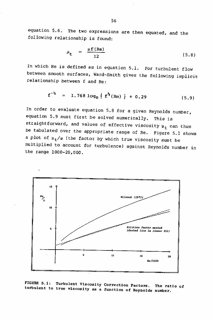
56
equation 5.6. The two expressions are then equated, and the following relationship is found:
At = j.tf(Re)
12 (5.8)
In which Re is defined as in equation 5.1. For turbulent flow
between smooth surfaces, Ward-Smith gives the following implicit relationship between f and Re:
f = 1.768 loge { f(Re) } + 0.29 (5.9)
In order to evaluate equation 5.8 for a given Reynolds number,
equation 5.9 must first be solved numerically. This is straightforward, and values of effective viscosity u t can thus be tabulated over the appropriate range of Re. Figure 5.1 shows
a plot of u/ (the factor by which true viscosity must be
multiplied to account for turbulence) against Reynolds number in the range 1000-20,000.
ts
Wilcock
.
1977
to
S friction factor method (dashed line Is linear fit)
to 20
Re/1000
FIGURE 5.1: Turbulent Viscosity Correction Factors. The ratio of turbulent to true viscosity as a function of Reynolds number.

57
Also shown in figure 5.1 is a curve corresponding to Wilcocks
correction factor which, for the reasons given above, is
included for order of magnitude comparisons only. To simplify
the analysis, a linear fit is now made to the curve in figure
5.1 (see dashed line) such that:
At = j.L(1+czRe) (5.10)
where:
a = 4.5x10 4
This linear relationship has the desirable characteristic that
at Reynolds number zero, p t is equal to ii. This is important, as regions of the lubricating film have zero Re at all times: a
relationship such as equation 5.5 would not take account of this
condition. Expression 5.10 is now used to substitute for i in
the lubrication-theory governing equation (equation 4.7), and
the damping analysis of section 4.4 then proceeds, otherwise as before.
A new expression for the damping coefficient, C (turbulent), is
thus obtained, which is related to the lubrication theory value C (laminar) according to:
C (turbulent) = C (laminar) + flE (5.11)
where:
Tj = 32apbr2
m2 A 3
and, assuming the same provisional bearing dimensions as so far
used:
1) = 7.11 x 10¹² kg (5.12)
W.
The second term in equation 5.11, ie. that arising from
turbulent considerations, will be of the same order as
C (laminar) when dimensionless velocity E equals C (laminar)/q.
Using equation 4.16 for C (laminar), this then corresponds to
velocity E = 0.0025, which lies between the two values predicted for Emax under rated-output loading (0.0014) and freakwave
loading (0.014), though significantly closer to the first.
Because of the assumptions involved - equations 5.6 and 5.7
refer to steady, fully developed flow between plane parallel
surfaces, besides which the influence of orifice flow is again
ignored - and the unproven nature of the analytical precept, the
above result is to be treated as an order of magnitude estimate
only. However, the approximately similar magnitudes of laminar
and turbulent damping terms at a maximum approach velocity near
that of rated-output loading, suggest that turbulent lubrication
might usefully increase the load capacity of the bearing under these conditions.
5.4 Turbulent Power Loss
The power dissipated by the bearing at rated output working,
assuming a turbulent lubricating film, is hard to quantify. In
the simple treatment of chapter 4, a shear loss was calculated
using constant viscosity (equation 4.23), and assuming laminar
conditions. It would be incorrect simply to replace the laminar
viscosity term with a turbulent equivalent found from the
analysis in section 5.3: there, the effective viscosity' was
derived for a turbulent Poiseuille flow regime, whereas the
bearing power loss actually occurs as the result of surface
shear. Similarly, using an effective viscosity based on the
model of eg. Wilcock (see section 5.3), neglects the fact that
in the present case turbulence does not result from shear. A
tentative estimate of power loss is therefore made in the
following way. The maximum film Reynolds number (ie. with peak
bearing velocity, and evaluated at 9 = r/2) under rated output
conditions is calculated on the basis of both pressure flow and
59
shear flow criteria. The former was above noted to be 1460, the
latter, based on a mean clearance h = 3 mm, and surface shear
velocity v = 5 m/s, has a value of 7500. Using the higher of
these, an effective viscosity is then read from the upper curve
in figure 5.1 (after Wilcock); the turbulent viscosity is found
to be approximately eight times the laminar value. Using
equation 4.23 as before, save for the substitution of the
turbulent viscosity term, gives a new estimate for power dissipation:
Turbulent power loss = 1.6 kW (5.13)
Although nearly an order of magnitude greater than that found
assuming lubrication theory, this is still a negligible loss,
representing only 0.07% of the ducks output.
Note that in the above example, peak bearing velocities are used
to estimate Reynolds number, but rms values inserted in the
equation for shear loss. This is intended to give a
conservative estimate for the increase in effective viscosity,
by accomodating the uncertainties which exist in the analysis
(see above).
5.5 The Influence of Fluid Inertia
The influence of fluid inertia on bearing performance can be
divided into direct and indirect, of which the latter is of
much greater importance in enhancing load capacity.
The significance of the direct effect can be roughly estimated
by calculating the mean dynamic pressure head-of the fluid film as 1/2 p0 2 at 0 = ir/2 (where its maximum value occurs) for the
two cases of freakwave and rated-output loading. Assuming the
mean clearance h = 3 mm, the maximum dynamic pressures in each
case are found, respectively, as 12 kPa and 0.12 kPa. These
figures represent 23% and 2.3% of the corresponding maximum
bearing pressures (as calculated in section 4.11); assuming the
AC
extra force required to accelerate the fluid corresponds to an
increase in load capacity, then, while inertial effects might
directly enhance bearing performance in the most extreme waves,
they appear to be of little significance under normal operating
conditions.
The indirect influence of fluid inertia arises because dynamic
pressures, although low compared with overall film pressure, can
be of the same order as the spring pressures acting on the two
sides of the magnet sheet. These in turn determine the
bearings damping characteristics, by controlling the film
thickness to hard clearance ratio h/H. A small imbalance in
pressure across the sheet, causing the narrow clearance to close
down by, say, a millimetre, from an equilibrium value of 3 mm,
would increase the local flow impedance by a factor greater than
three; this results from the inverse-cube law for lubrication
flow. Exactly such a fluid pressure imbalance is caused when
the water in the compliant lining is squeezed out through the
sheet orifices into the clearance: inside the lining the fluid
is at rest, and the increase in its velocity on entering the
lubricant film is accompanied by a drop in static pressure,
corresponding to the acquisition of its dynamic (inertial) head.
The effect is greatest in those areas of the bearing discharging
the most water, ie. closest to the effective load application
point (9 = 01, and here will be observed the greatest increases
in local load capacity.
Not only does this characteristic of fluid inertia potentially
increase the overall load capacity of the bearing, it also gives
it an asymmetric response, offering a large reduction in the
amount of magnetic material required (see section 4.12). An
asymmetric response will occur because no pressure imbalance of
the kind described above exists on the negatively loaded side of
the bearing, where water is being drawn from the lubricating
film back into the compliant lining. In this region, the
dynamic pressure head of the fast-moving fluid is effectively
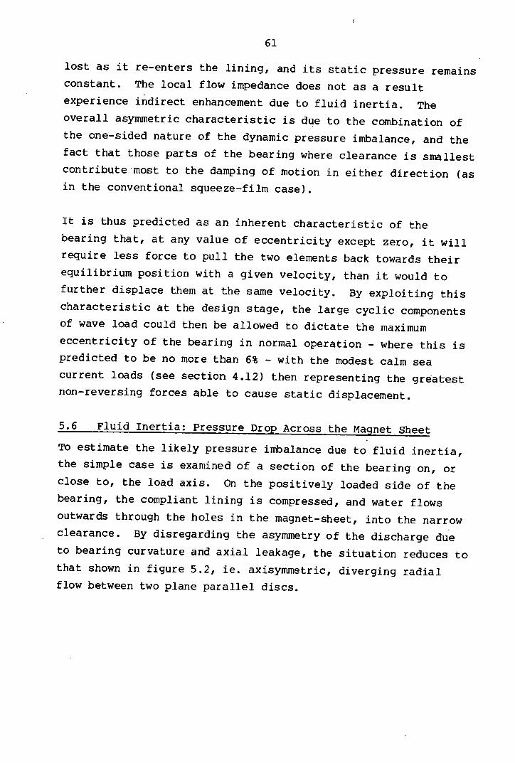
61
lost as it re-enters the lining, and its static pressure remains
constant. The local flow impedance does not as a result
experience indirect enhancement due to fluid inertia. The
overall asymmetric characteristic is due to the combination of
the one-sided nature of the dynamic pressure imbalance, and the
fact that those parts of the bearing where clearance is smallest
contribute most to the damping of motion in either direction (as
in the conventional squeeze-film case).
It is thus predicted as an inherent characteristic of the
bearing that, at any value of eccentricity except zero, it will
require less force to pull the two elements back towards their
equilibrium position with a given velocity, than it would to
further displace them at the same velocity. By exploiting this
characteristic at the design stage, the large cyclic components
of wave load could then be allowed to dictate the maximum
eccentricity of the bearing in normal operation - where this is
predicted to be no more than 6% - with the modest calm sea
current loads (see section 4.12) then representing the greatest
non-reversing forces able to cause static displacement.
5.6 Fluid Inertia: Pressure Drop Across the Magnet Sheet
To estimate the likely pressure imbalance due to fluid inertia,
the simple case is examined of a section of the bearing on, or
close to, the load axis. On the positively loaded side of the
bearing, the compliant lining is compressed, and water flows
outwards through the holes in the magnet-sheet, into the narrow
clearance. By disregarding the asymmetry of the discharge due
to bearing curvature and axial leakage, the situation reduces to
that shown in figure 5.2, le. axisyminetric, diverging radial
flow between two plane parallel discs.
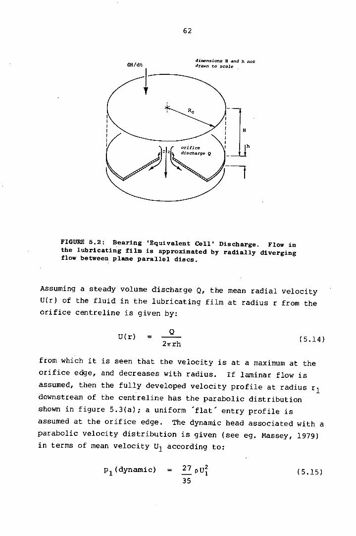
dimensions H and h not drawn to scale
1 1 H C orifice
I
FIGURE 5.2: Bearing 'Equivalent Cell' Discharge. Flow in the lubricating film is approximated by radially diverging flow between plane parallel discs.
Assuming a steady volume discharge Q, the mean radial velocity
U(r) of the fluid in the lubricating film at radius r from the orifice centreline is given by:
U(r) = Q
2w rh (5.14)
from which it is seen that the velocity is at a maximum at the
orifice edge, and decreases with radius. If laminar flow is
assumed, then the fully developed velocity profile at radius r l downstream of the centreline has the parabolic distribution
shown in figure 5.3(a); a uniform flat entry profile is
assumed at the orifice edge. The dynamic head associated with a
parabolic velocity distribution is given (see eg. Massey, 1979) in terms of mean velocity U 1 according to:
dH/dt
p1(dynamic) = 27 p U 2 (5.15)
35
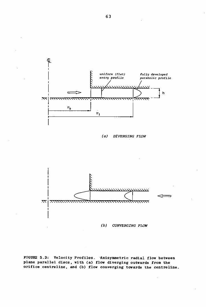
uniform (flat) entry profile
=I1 r j ;1
63
fully developed parabolic profile
(a) DIVERGING FLOW
(b) CONVERGING FLOW
FIGURE 5.3: Velocity Profiles. Axisymmetric radial flow between plane parallel discs, with (a) flow diverging outwards from the orifice centreline, and (b) flow converging towards the centreline.
Ir

64
The drop in static pressure between a point inside the lining
(where static pressure is taken to equal stagnation pressure)
and the fully developed flow at r 1 is then given by:
27 2 = _pU 1 + AP 01 (v1scous) 35
(5.16)
where tp0,1 (viscous) occurs between radii r 0 and r 1 . If the flow were fully developed, with a parabolic rather than flat, profile at r 0 , then:
Po,i (viscous) = 6Q- log e I r0 (5.17)
which represents the classical lubrication-theory pressure loss for axisymmetric radial flow (Rayleigh, 1917). This
underestimates the actual loss, as a uniform entry profile at r 0 entails higher (theoretically infinite) shear stresses at the
channel walls. However, if full development of the velocity
profile occurs close downstream of the orifice edge without
significant viscous loss, the dynamic pressure head, and hence static pressure drop, can be approximated by:
p (dynamic) = . Z p u 2 35 0 (5.18)
where U0 is the mean velocity at the orifice edge. This
assumption has previously been employed by Kawashima (1976,
1978) to account for the observed pressure drop in radial-flow hydraulic valves.
A different estimate has been proposed by Mori and Yabe (1966)
based on a momentum-theorem calculation, whereby the increased
momentum of the parabolic, compared with the uniform, velocity
profile is equated with a pressure drop of 1/5 ptJ, giving
the net dynamic head on entry as:
p1 (dynamic) = (Mori & Yabe, 1966) (5.19) 10

65
Another estimate has been made by Vohr (1969), based on
integration of the momentum across the width of the parabolic
profile, with resulting dynamic head term:
p1 (dynamic) = 3 P (Vohr, 1969) (5.20)
Of the three estimates, the first - and highest - appears most
strictly correct, as it assumes nothing about the losses
incurred in the developing profile between r 0 and r 1 .
The magnitude of the orifice static pressure drop in the
'discharging' regions of the proposed bearing is a design
parameter of potentially fundamental importance. In the next
chapter are presented the results of experiments which were
undertaken to confirm the appropriate governing equation for
this pressure drop, and to demonstrate how, by a suitable choice
of orifice geometry, the phenomenon of flow separation can
significantly enhance its magnitude.
5.7 Convergent Radial Flow
Consider now the case where the section of the bearing
illustrated in figure 5.2 is negatively loaded: the compliant
lining recharges, drawing water in from the lubricating film.
Making the same assumptions as in section 5.6, the water in the
clearance now flows radially inwards, converging towards the
orifice. The subsequent deceleration to stagnation conditions
results in turbulent loss of the entire dynamic pressure head,
with the static pressure inside the lining equal to that in the
radial film at the orifice edge. This phenomenon has been
experimentally demonstrated by McGinn (1955) and in the present
work (see section 6.4).
Figure 5.3(b) shows the velocity profile of the converging
radial flow. With a fully developed parabolic profile at
the loss of dynamic head is strictly that given in equation
5.18. Although there is some experimental evidence of a partial
M.
head recovery on the lower wall at the centreline (see section
6.4), this is purely a boundary effect, and is not reflected in the pressure measured above the orifice.
The asymmetric behaviour of the overall bearing arises because
of the 'inertia-paradox' of axisymrnetric radial flow: .in
divergent (outward) radial flows, conservation of total pressure
leads to a drop in static pressure across the orifice, while in
convergent flows, loss of total pressure results in the
conservation of static pressure.
5.8 The Importance of the Inertial Pressure Imbalance
If each orifice in the magnet-sheet discharges/recharges the
water contained in a volume of the compliant lining equivalent to a 'cell' of plan area irR, as shown in figure 5.2, then the volume flowrate through the orifice is given by:
Q = ±RdH/dt (5.21)
and hence from equation 4.1:
Q = ± irR2 e cos e (5.22)
where is the hard-surface approach velocity. The mean radial
fluid velocity at the orifice edge, considering only the flow
due to discharge of the particular cell being considered, is
then found from equations 5.14 and 5.22 as:
U0= _______ (5.23) 2r 0 h
The resulting static pressure drop across the orifice in
diverging radial flow is then found using this expression to substitute for U0 in equation 5.18, hence:
AP (dynamic) = --LpRk 1 eCOSe }2 (5.24) 140 C r0h

67
In section 4.5 it was shown that the dominance of fluid damping
dictates that velocity é is proportional to applied load, with
the damping coefficient inversely proportional to the cube of
the film thickness h (equation 4.17). Hence, from equation 5.24:
F0 cose Ap (dynamic) cc
{
} 2 (R h)" r0 C (5.25)
Superficially, then, and ignoring all nonlinearities,
turbulence, etc., the dynamic pressure imbalance increases with
the fourth power of clearance h, in contrast to the overall
impedance (hence load capacity) of the bearing, which decreases with h 3 . The two effects are in a way opposed: the former
causes a narrowing of the clearance on the positively loaded
side of the bearing, while the latter resists the approach of the two surfaces.
The fact that these opposing effects are governed by high powers
of clearance h, with the first decreasing and the second
increasing under positive loading, should be exploited from the
outset in the bearing design. Its operating characteristics
might then be significantly different from those assumed in the
simple analysis in chapter 4. A greater equilibrium clearance
would be possible, which on the application of a dynamic load
would rapidly close down to a safe minimum working value, as the
dominance of inertial pressure imbalance and overall impedance
changed hands. As a result of the high-order dependence on h of
these two characteristics, the working clearance would be
maintained within a very narrow band. Utilising this, the
indirect influence of fluid inertia, to maximum effect would
largely be a matter of incorporating in the design of the
bearing the optimum combination of magnetic and compliant lining
stiffnesses, lubricating film thickness, and overall hard'
clearance.
Although no attempt to obtain the ideal combination has yet
been made, the task seems eminently feasible, as small changes
in the above parameters yield much larger ones in the desired
effect. To demonstrate the available design latitude, the
influence of equilibrium film thickness h on the dynamic
pressure imbalance can be shown by referring to the
'equivalent cell' in figure 5.2. Assuming an orifice radius r 0 of 5 mm, with cell radius R c of 100 mm, then under freakwave loading (I = 0.002 m/s) the maximum dynamic head is found from equation 5.24, with:
p (dynamic) = 375 Pa (5.26)
This pressure may be quite low in comparison to the magnetic
repulsion pressure against which it is required to act;
however, by doubling the equilibrium clearance to 6 mm, the
above figure rises sixteen-fold to 6.0 kPa, which may well be
too high to allow. The appropriate clearance would then obviously lie between the two figures.
The advantage of a large equilibrium film thickness is to allow
the use of less magnetic material, because the greater
available change in working clearance then allows a less stiff
magnetic repulsion system to be employed to provide the minimum
calm-sea static load. A rough guess at the possible magnet
reduction assumes the amount required to be inversely
proportional to the equilibrium clearance, ie. doubling h in
the above example might potentially halve the weight of magnets
needed. One characteristic to be avoided, however, is a
too-great dynamic pressure imbalance acting on the compliant
magnet-sheet, which might lead to localised grounding around
the discharging orifices (although the corresponding local
increase in flow impedance might prevent this occurrence).
WO
5.9 The Complete Flow Field
The simple radial flow patterns described above might be
observed in the region of the load axis, but elsewhere, the
overall flow pattern will be a much more complex combination of
orifice flow and the main flow of the lubricating film. The
ratio of orifice discharge (or recharge) flow to the total flow
past a section at angle e to the load axis is given by:
%rif ice = lrRc (5.27)
total 2r tan8
which decreases to zero at 90. 0 to the axis, there being no
lining compression in this region.
A possible model of the complex flow field is suggested by the
work of Mori and Yabe (1967), who examined the case of a
rectangular thrust bearing with multiple supply holes. In their
treatment, the assumptions are made of (a) constant clearance,
(b) negligible surface velocity, and (c) constant fluid
viscosity: under these conditions, Reynolds equation (which
governs the flow of a classical' lubricant) reduces to
Laplaces equation, ie.:
(5.28) dx2 dy 2
which is then solved using complex potential theory. Although
the method neglects fluid inertia in the film, a correction is
included to allow for the pressure drop at the orifice edges
(see equation 5.19) due to development of the dynamic head.
If the above assumptions (a-c) were made for the present
bearing, this technique could be applied to obtain a more
accurate picture of its pressure/flow characteristics. Indeed,
the closed nature of the system may well make it a simpler
analytical problem than that of the rectangular bearing. The
necessary assumption of constant film thickness defines the net
flow in the clearance to be always zero, and entirely accounted

70
for by real point sources and sinks, in the form of the sheet
orifices: in contrast to the rectangular thrust bearing case, no
additional sinks need be defined to satisfy the boundary
conditions. The necessary pressure-loss correction for
discharging orifices is given in equation 5.18, and no
correction is needed for recharging orifices: analytic
distinction between the two is simple, based on position
relative to a diametric line at right angles to the load axis.
Total discharge is directly proportional to approach velocity .
Although no start has yet been made on such an analysis, it is
strongly recommended as the next theoretical step.
The most complete analysis of all would have to take account of
nonlinear stiffness, non-constant clearance (including
compliance), film fluid inertia and turbulence, squeeze-film
effects, and unsteady flow. A representative experimental model seems a more attractive proposal.
5.10 Conclusions
The water in the lubricating film will have complex flow
characteristics, with both turbulence and fluid inertia
influencing overall bearing performance. Turbulent lubrication
will give rise to increases in both load capacity and power loss
compared with those found from the earlier lubrication theory. analysis. However, load enhancement will probably be of
significance only in extreme waves, and power loss is still
estimated as less than 0.1% of the ducks rated output.
The direct influence of fluid inertia will be load enhancing,
but is likely to contribute little under normal working
conditions. Its indirect influence, represented by the pressure
drop across the discharging magnet-sheet orifices, is of much
greater significance: this can potentially give rise to greatly
increased load capacity, and also endow the bearing with a
favourably asymmetric response. The key to the latter
characteristic is the lack of a similar pressure drop across the
71
recharging orifices. Based on the model of axisymmetric
(laminar) radial flow, the static pressure drop across a
discharging orifice is estimated as 27/35pU, where U O is the mean radial fluid velocity at the orifice edge. By exploiting
the indirect effect of fluid inertia, it is proposed that large
reductions can be made in the magnet requirement.
A detailed analysis of the lubricating film flow-field in the
bearings narrow clearance is suggested (though not carried out)
on the basis of previously published work: the analysis would
take account of the components of flow in the overall
lubricating film due to local orifice discharge/recharge,
including inertial effects, and might yield a more accurate
description of the bearings performance characteristics.
72
CHAPTER 6
RADIAL FLOW EXPERIMENTS
6.1 Chapter Summary
Experiments, which were designed to demonstrate the important
features of the indirect influence of fluid inertia in the
proposed bearing, are described. The experimental model used
was that of steady, axisyininetric radial flow between plane
parallel discs. To simulate both discharge and recharge of
water through the sheet-orifices in the the bearing lining,
divergent and convergent radial flows were used. Radial
pressure distributions were measured for both cases, over the same range of volume flowrates.
The governing law for the orifice pressure loss in diverging
flows is investigated by examining the measured pressure losses,
expressed dimensionlessly, as a function of the reduced Reynolds number Rex , while the asymmetry of the effect is demonstrated in
a qualitative comparison of the results for diverging and
converging flows. A qualitative investigation of the influence
of orifice geometry is also made, paying particular regard to
the phenomenon of flow separation. The experimental apparatus,
its novel features and operational limitations, are fully
described, including a load cell, and a pressure calibration
device, both of which operate on the same principle as a hydrostatic bearing.
6.2 Experimental Apparatus
The experiments were designed to give pressure variations of
accurately measurable size. Because the orifice discharges in
the full scale bearing depend greatly on position relative to
the load axis, and on the loading regime, experimental
conditions were representative of only a small part of the full
range, namely that characterised by low values of reduced
Reynolds number Rex (see section 6.5). The range of Rex,
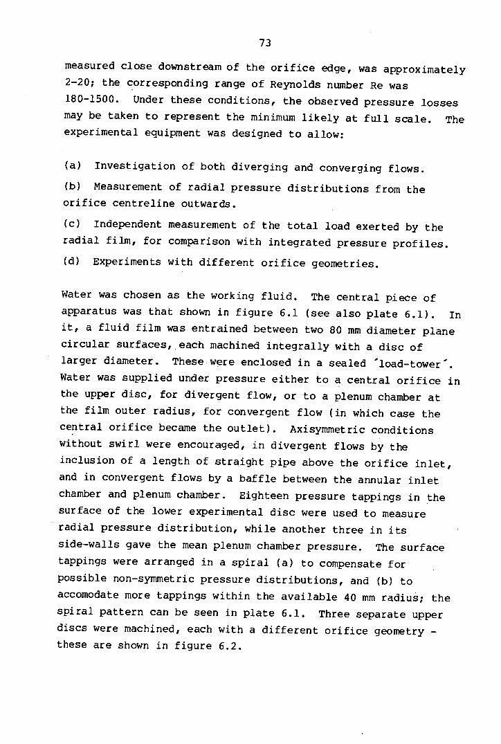
73
measured close downstream of the orifice edge, was approximately
2-20; the corresponding range of Reynolds number Re was
180-1500. Under these conditions, the observed pressure losses
may be taken to represent the minimum likely at full scale. The experimental equipment was designed to allow:
Investigation of both diverging and converging flows.
Measurement of radial pressure distributions from the orifice centreline outwards.
Independent measurement of the total load exerted by the
radial film, for comparison with integrated pressure profiles.
Experiments with different orifice geometries.
Water was chosen as the working fluid. The central piece of
apparatus was that shown in figure 6.1 (see also plate 6.1). In
it, a fluid film was entrained between two 80 mm diameter plane
circular surfaces, each machined integrally with a disc of
larger diameter. These were enclosed in a sealed load-tower'.
Water was supplied under pressure either to a central orifice in
the upper disc, for divergent flow, or to a plenum chamber at
the film outer radius, for convergent flow (in which case the
central orifice became the outlet). Axisymrnetric conditions
without swirl were encouraged, in divergent flows by the
inclusion of a length of straight pipe above the orifice inlet,
and in convergent flows by a baffle between the annular inlet
chamber and plenum chamber. Eighteen pressure tappings in the
surface of the lower experimental disc were used to measure
radial pressure distribution, while another three in its
side-walls gave the mean plenum chamber pressure. The surface
tappings were arranged in a spiral (a) to compensate for
possible non-symmetric pressure distributions, and (b) to
accomodate more tappings within the available 40 mm radius; the
spiral pattern can be seen in plate 6.1. Three separate upper
discs were machined, each with a different orifice geometry - these are shown in figure 6.2.
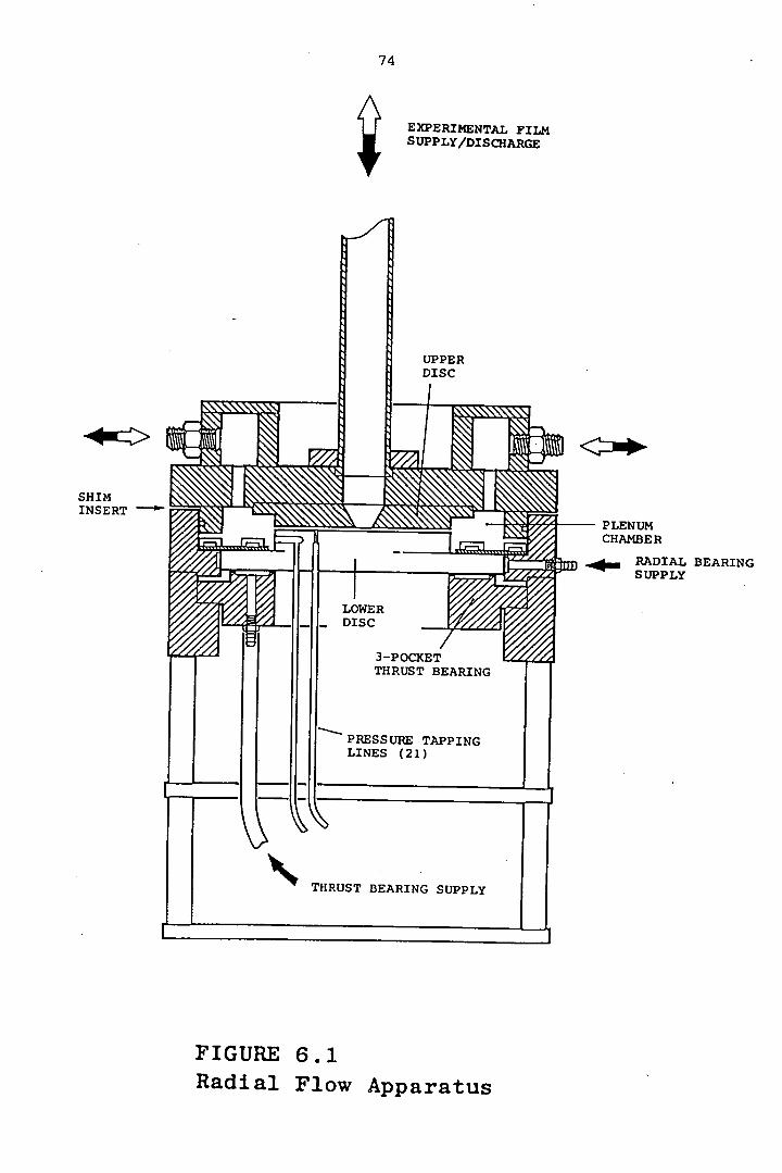
EXPERIMENTAL FILM SUPPLY/DISCHARGE
74
SHIM INSERT -
PLENUM CHAMBER
RADIAL BEARING SUPPLY
FIGURE 6.1 Radial Flow Apparatus
OVERLEAP
PLATE 6.1 Radial Flow Apparatus. The lower experimental disc (foreground) is supported by a 3-pocket water-fed thrust bearing, or 'hydrostatic load cell', enclosed in the main load-tower apparatus (background). Centralisation of the disc is by a 3-pocket radial bearing. Note the spiral of pressure tappings in the upper surface of the disc.
75
FOLLOWING PAGE
PLATE 6.2 Hydraulic Impedances. Screw-cut impedances of the kind shown were used to supply both load cell hydrostatic bearings. The parallel-capillary core (foreground) was designed to enable high flowrates of low viscosity lubricant (water) at low Reynolds number, thus avoiding nonlinear characteristics. Each core is enclosed in a shim-reinforced heatshrink sandwich (background).
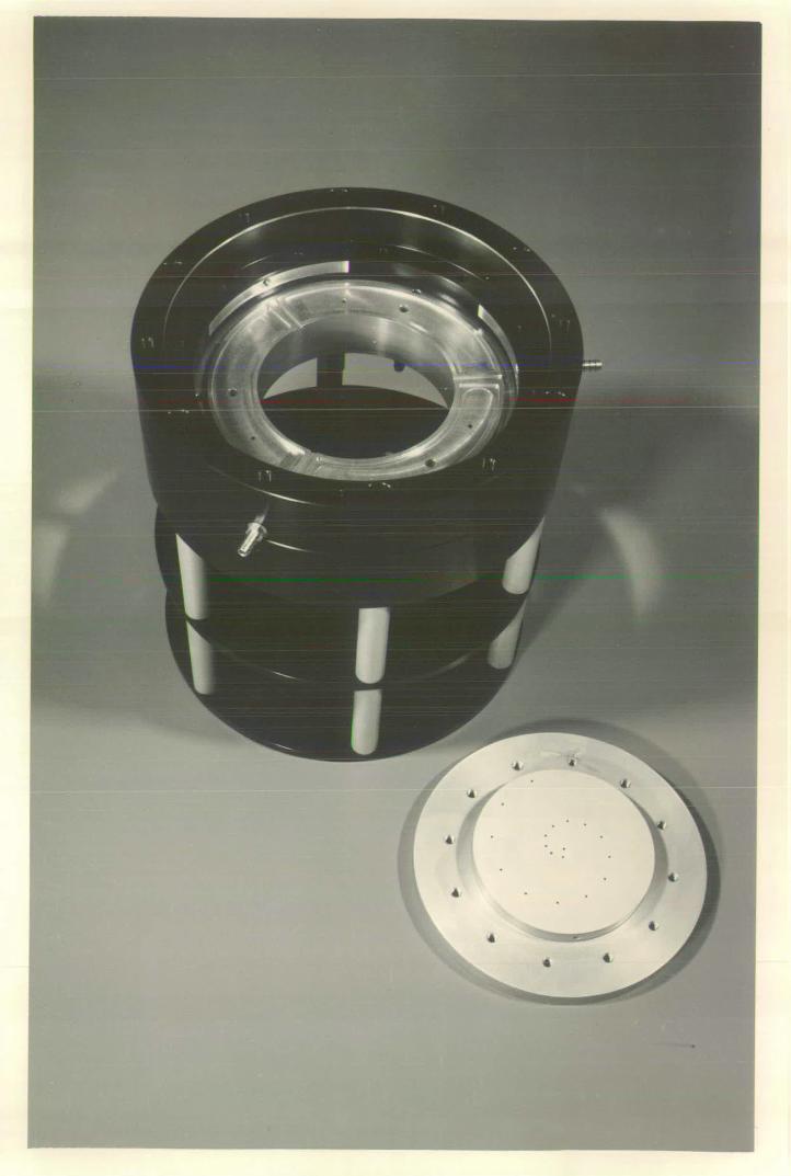
1~
. .
7 : lI_
.Mai

t
11 P's

W.
attachment flange
__ \
/ 60.50 I ______________ film ____ Outer
1J L A radius
/.\81.l0 I I
16
123.5 0 I
8 L 32
0
DIMENSIONS IN mm
FIGURE 6.2
Experimental Orifice Geometries
GEOMETRY r0 /R
01 0.1
02
0.2
04
0.4
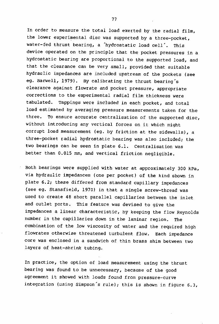
77
In order to measure the total load exerted by the radial film,
the lower experimental disc was supported by a three-pocket,
water-fed thrust bearing, a 'hydrostatic load cell'. This
device operated on the principle that the pocket pressures in a
hydrostatic bearing are proportional to the supported load, and
that the clearance can be very small, provided that suitable
hydraulic impedances are included upstream of the pockets (see
eg. Barwell, 1979). By calibrating the thrust bearings
clearance against flowrate and pocket pressure, appropriate
corrections to the experimental radial film thickness were
tabulated. Tappings were included in each pocket, and total
load estimated by averaging pressure measurements taken for the
three. To ensure accurate centralisation of the supported disc,
without introducing any vertical forces on it which might
corrupt load measurement (eg. by friction at the sidewalls), a
three-pocket radial hydrostatic bearing was also included; the
two bearings can be seen in plate 6.1. Centralisation was
better than 0.015 mm, and vertical friction negligible.
Both bearings were supplied with water at approximately 300 kPa,
via hydraulic impedances (one per pocket) of the kind shown in
plate 6.2; these differed from standard capillary impedances
(see eg. Stansfield, 1970) in that a single screw-thread was
used to create 48 short parallel capillaries between the inlet
and outlet ports. This feature was devised to give the
impedances a linear characteristic, by keeping the flow Reynolds
number in the capillaries down in the laminar region. The
combination of the low viscosity of water and the required high
flowrates otherwise threatened turbulent flow. Each impedance
core was enclosed in a sandwich of thin brass shim between two
layers of heat-shrink tubing.
In practice, the option of load measurement using the thrust
bearing was found to be unnecessary, because of the good
agreement it showed with loads found from pressure-curve
integration (.using Simpson's rule); this is shown in figure 6.3,
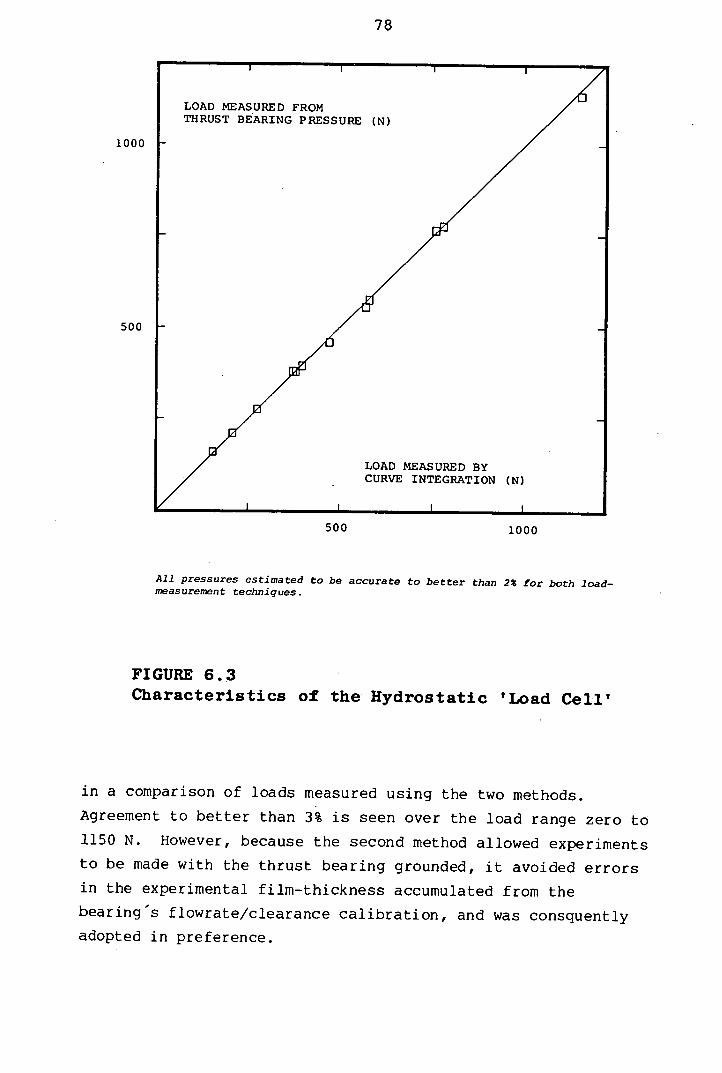
78
LOAD MEASURED FROM THRUST BEARING PRESSURE (N)
1000
500
LOAD MEASURED BY CURVE INTEGRATION (N)
500 1000
All pressures estimated to be accurate to better than 2 for both load-measurement techniques.
FIGURE 6.3 Characteristics of the Hydrostatic 'Load Cell'
in a comparison of loads measured using the two methods.
Agreement to better than 3% is seen over the load range zero to
1150 N. However, because the second method allowed experiments
to be made with the thrust bearing grounded, it avoided errors
in the experimental film-thickness accumulated from the
bearing's flowrate/clearance calibration, and was consquently
adopted in preference.
79
The entire.load tower was fabricated from aluminium alloy, with
all parts anodised for corrosion protection. Opposing disc and
thrust-bearing surfaces were hand-lapped to near optical finish
before being anodised. No visible degradation of these surfaces occurred in use.
6.3 Pressure and Flow Measurement
Pressure measurements were made using a solid-state transducer
(RSComponents Ltd), with nominally linear output in the range
0-30 psi (207 kPa). To achieve maximum accuracy, and also allow
operation up to its maximum rating of 60 psi (414 kPa), the
transducer was calibrated using the device illustrated in figure
6.4. This again used the hydrostatic bearing principle: a
centralised, freely-sliding plunger was levitated by the
pressure of water in the pocket below, which was governed by the
addition of calibrated weights to the top-plate. The transducer
was calibrated over the range 0-372 kPa (54 psi), with the
calibration procedure showing repeatability better than 1%. The
calibration curve was stored in memory in a CBM 4032
microcomputer, to which the transducer was interfaced via A/D
converter (PCI 6300, CIL Microsystems), allowing direct reading
and recording of pressures.
All tappings were connected by PVC tubing to a 36-way hydraulic
selector switch. This employed a bonded PTFE face seal to
connect selectively the required tapping line to the pressure
tranducer, while blocking off all the others. Each recorded
pressure was the mean of 40 samples taken over a 5-second
period, and individual pressure distribution curves were
averaged from six nominally identical experiments, each made
with the upper disc rotated 60 0 from its previous position. This procedure was introduced to compensate for non-parallellism
of the experimental plates; parallellism was estimated as 3-8
microns, where the latter figure, although small, represented
10% of the film thickness in one experiment.
CALIBRATED WEIGHTS
LY-SLIDING GER
INE TO BESS URE TRANSDUCER
S UP PLY
PTFE BUSH
PTFE GUIDES
FIGURE 6.4 Hydrostatic Calibrated-Pressure Source
The water supply for all aspects of the apparatus came from a
60 psi (400 kPa) domestic main. Random pressure fluctuations of
up to 4% were observed, but by time averaging the measurements
(see above) this figure was effectively reduced to less than 1%.
The supply was filtered upstream of all experimental apparatus,
using a Microwynd 50 pm fibre element, but otherwise was
untreated. Flowrates were determined by collection and
weighing, with an accuracy of better than 0.25%. Temperature
was monitored to within 0.3 CO during each experiment, to correct for viscosity variations.
6.4 Experimental Results
Each experiment involved an averaged measurement (see section
6.3) of the radial pressure distribution in the fluid film, for
a given combination of plate separation, inlet pressure, flow
direction, and orifice geometry; the three experimental
geometries (shown in figure 6.2) had radius ratios r 0/R = 0.1, 0.2, and 0.4. Typical results for these are shown in figures
6.5 - 6.7; note that the points are joined to show the form of
each experimental curve: these are not theoretical comparisons.
In all cases, plenum chamber pressure is taken as the datum, and
hence the converging flow pressures are depicted as negative.
This is purely for convenience: all measured pressures were
positive. Note that the true zero pressure for converging
flows, corresponding to that measured in the outlet pipe, does
not correspond to the reading at zero radius, but to the lowest
reading shown in each case (see section 6.5). The values of
plate separation h are based on a theoretical fit of equation
6.3 (see section 6.5) to the lowest (diverging) flowrate curve,
and differ by up to 10% from nominal estimates made on the basis
of the pre-assembled load-cell dimensions. Although the value
of h found in each case is thought to be more accurate than
nominal (the same technique is used in air-gauging), this
applies only to diverging flows.

PRESSURE (kPa)
1eIi B
100 C
ro 10
DI/
plate separation h = 100 Am*
orifice radius r 0 = 4 mm
curve Q (cm 3 /s) t (cP)
A + 55.28 1.12
B + 31.30 1.12
C + 16.23 1.07
D - 16.96 1.11
E - 31.73 1.11
*(from theoretical fit to curve 'C'
DIVERGING FLOW
IL Re' = 1.16
radius (mm)
CONVERGING FLOW
V.!
ME
40
-loo t
El
-200
Pressures estimated accurate to better than 2%
FIGURE 6.5 Radial Flow Results: Orifice 01
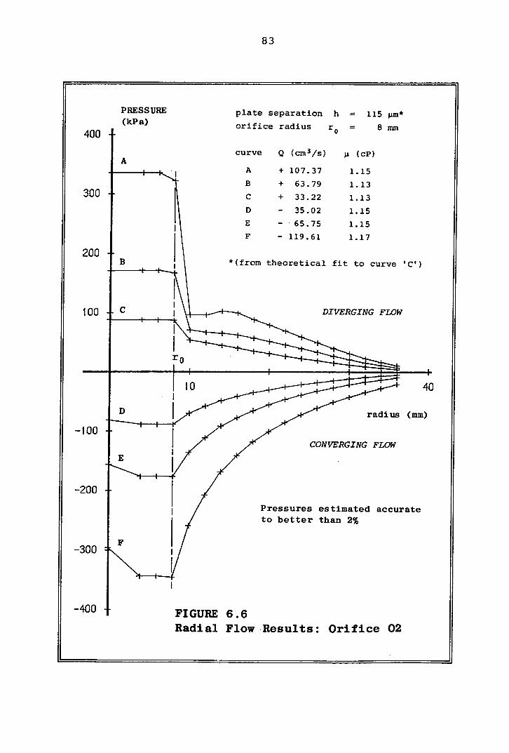
83
PRESSURE (kPa)
400
A
300
J I
200 + lB
plate separation h = 115 pm*
orifice radius r 0 = 8 mm
curve Q (cm 3 /s) i (cP)
A + 107.37 1.15 B + 63.79 1.13 C + 33.22 1.13 D - 35.02 1.15 E - 65.75 1.15 F - 119.61 1.17
*(from theoretical fit to curve 'C')
100 -I- C
DIVERGING FLOW
D
-100
E
-200
-300 F
r o
t--,+O-
MA
40
radius (mm)
CONVERGING FLOW
Pressures estimated accurate to better than 2%
400 FIGURE 6.6 Radial Flow Results: Orifice 02

84
PRESSURE plate separation h = 108 pm*
(kPa) orifice radius r0 = 16 nun
curve Q (czn 3/s) i (cP)
300 A + 161.73 1.16 A B + 88.70 1.15
C + 46.62 1.14 D - 51.19 1.15 E - 96.45 1.15 F - 175.02 1.17
200 *(from theoretical fit to curve 'C')
B
I DIVERGING FLOW 100
10 40
------I
r
ofTiii::iiii:ii:::i:i -100
radius (mm)
CONVERGING FLOW
-200
F Pressures estimated accurate to better than 2%
-300 ,
FIGURE 6.7 Radial Flow Results: Orifice 04
Clearance errors were incurred in some converging flow
experiments, due to plate deflections caused by high pressure
water acting on a much greater internal area of the assembly
(see figure 6.1) than in diverging flow experiments. In the
worst case, a theoretical curve-fit indicated 25 i.tm clearance
deflection (for a disc thickness of 20 mm): the total fluid load
in the experiment was about 4000 N at the time. For the same
inlet pressure in diverging flow, a load of only 400 N applied,
and deflection was negligible. Despite this, the high-pressure
converging flow results are retained, as useful observations can
be made from them (see section 6.5, and (2) below).
The main qualitative points to note in figures 6.5 - 6.7 are:
In all cases, the pressure difference from the orifice edge, radius r 0 , to the first tapping outwards, radius r 1 , is greater in diverging flows than in converging flows of similar
flowrate, and the discrepancy increases strongly with flowrate.
In converging flows, the pressure drop is accounted for by the
sum of the viscous loss and increased dynamic head going from r l inwards to r0 . In diverging flows these two effects act in
opposition (with theoretical recovery of dynamic head between r o and r1) to produce a smaller contribution to the net pressure
drop. However, a large extra loss is incurred due to
development of the velocity profile from initial stagnation
conditions (see figure 5. 3), and this represents the
fundamental inertial pressure imbalance described in sections
5.5 - 5.8. It occurs only in diverging flows, and its magnitude
is estimated in section 6.5.
In high flowrate converging flows (eg. curve F, figure 6.7)
a head loss is seen at the film entry, ie. the disc outer radius
(radius = 40 mm). This effect is exactly analogous to that
described above, and is associated with development of the
velocity profile from the stagnation conditions existing in the
plenum chamber.
AM
Diverging flow curves measured at high flowrates tend to be
unsmooth, in contrast to similar converging flows. Although
viscous/inertial theory predicts non-symmetry for the two cases,
in the sense that they would not superimpose if reflected
through the axis of zero pressure, the diverging curves might be
expected to become smooth at large radii, where viscous effects
dominate. A possible explanation is that turbulence and/or flow
separation is carried downstream from the region of the orifice
edge, where strongly adverse pressure gradients exist (in
diverging flows only).
In all converging flow cases, the pressure measured at the
orifice centre (radius zero) is seen to be greater than at the
orifice edge, demonstrating a partial recovery of dynamic head.
However, the pressure measured in the outlet pipe above the
orifice was always found to correspond to the lowest film
pressure, suggesting that recovery was confined only to the
surface of the lower disc.
6.5 Quantitative Results Analysis
To quantify the component of the film entry pressure loss
associated with velocity profile development in diverging flows,
the measured pressure loss is examined as a function of the
reduced Reynolds number ReX. This is the most useful criterion
for dynamic similarity in lubrication analyses where the
influence of fluid inertia is important (see eg. Mime, 1965).
For axisymmetric radial flow, Re x is found as the product of Reynolds number Re and the film thickness ratio:
X Re = Re (h/r) (6.1)
where r is the radial distance from the radial symmetry axis.
Hence:
Re = x ph 2U
(6.2)
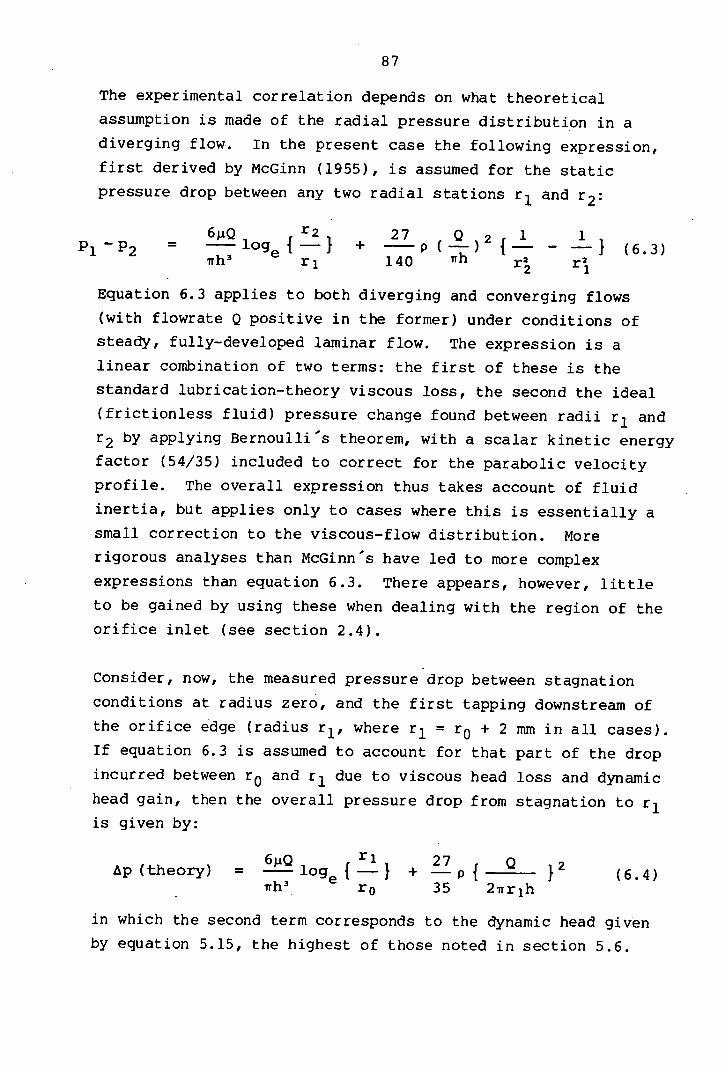
NE
The experimental correlation depends on what theoretical
assumption is made of the radial pressure distribution in a
diverging flow. In the present case the following expression,
first derived by McGinn (1955), is assumed for the static
pressure drop between any two radial stations r 1 and
6!iQ 2 27 Q = —log - + (_) 2 {L - ( 6.3)
7rh3 e r1 140 trh
Equation 6.3 applies to both diverging and converging flows
(with flowrate Q positive in the former) under conditions of steady, fully-developed laminar flow. The expression is a
linear combination of two terms: the first of these is the
standard lubrication-theory viscous loss, the second the ideal
(frictionless fluid) pressure change found between radii r 1 and r 2 by applying Bernoulli's theorem, with a scalar kinetic energy
factor (54/35) included to correct for the parabolic velocity
profile. The overall expression thus takes account of fluid
inertia, but applies only to cases where this is essentially a
small correction to the viscous-flow distribution. More
rigorous analyses than McGinns have led to more complex
expressions than equation 6.3. There appears, however, little
to be gained by using these when dealing with the region of the
orifice inlet (see section 2.4).
Consider, now, the measured pressure drop between stagnation
conditions at radius zero, and the first tapping downstream of
the orifice edge (radius r 1 , where r 1 = r0 + 2 mm in all cases). If equation 6.3 is assumed to account for that part of the drop
incurred between r 0 and r 1 due to viscous head loss and dynamic
head gain, then the overall pressure drop from stagnation to r 1 is given by:
6iQ r, 27 p (theory) = - loge { _ I + -') [ Q (6.4)
ir h 3 r 0 35 2iir 1 h
in which the second term corresponds to the dynamic head given
by equation 5.15, the highest of those noted in section 5.6.

If the pressure drop is now made non-dimensional according to:
p(dimensionless) &p / { } (6.5) 2 nh 3
then equation 6.4 becouths
27 p (dimensionless) = 12 loge { -
ro 1 + - ( Re 1 ) ( 6.6)
35
where Rex is the reduced Reynolds number (see equation 6.2)
evaluated at the downstream tapping radius r 1 . A plot of measured (dimensionless) pressure drop against Rex in theory
then gives a straight line of slope 27/35, ie. the predicted
pressure loss coefficient, and intercept 12 x log{r 1/r 0 }, a quantity depending only on the fixed orifice dimensions.
The experimental results are shown in figures 6.8 and 6.9. In
all cases the points lie along approximately straight lines,
indicating dimensionless pressure drop to increase linearly with
Rel . Pressure losses for orifices 01 and 02 are notably higher
than predicted at all Re t , but the gradient in both cases
agrees quite well with theory; in neither case does it suggest a
smaller pressure loss coefficient than that predicted above.
With orifice 04 the fit is good, in terms of both gradient and
intercept. This is a little surprising, as in this case
particularly, a fully developed velocity profile is unlikely to
have existed at the downstream tapping. The development-length
criterion of Schlichting (1979) can be applied (strictly it refers to non-radial flow, and other reasons exist for using it with caution - see Van Dyke, 1970), giving the following
expression for Ld, the distance downstream of the film entry at which full flow development may be assumed:
L O.O4xr1x(Re')
(6.7)
For orifice 04, with Re of 7.4, the value of L d is 5.3 whereas the tapping point at r 1 is only 2 mm downstream from

25
20
15
10
5
DIMENSIONLESS PRESSURE DROP
I UQ
ru
fl direction
ow
13 0
01
theoretical, assuming fully developed laminar profile
REDUCED REYNOLDS NUMBER Re
I I I
0
5 10 15 20
20
15
10
5
PRESSURE DROP
flow direction
al
02
theoretical, assuming fully developed laminar profile
REDUCED REYNOLDS NUMBER Re x
DIMENSIONLESS
0
5 10 15
FIGURE 6.8 Experimental Pressure Losses. Results for orifice geometries 01 (top) and 02 (bottom); see figure 6.9 for geometry 04.
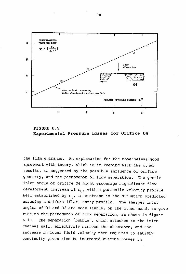
all
DIMENSIONLESS
8 PRESSURE DROP
Ap / uQ
2irh 3
6
4
2
flow direction
123.5-
04
theoretical, assuming fully developed laminar profile
REDUCED REYNOLDS NUMBER Re
2 4 6 8
FIGURE 6.9 Experimental Pressure Losses for Orifice 04
the film entrance. An explanation for the nonetheless good
agreement with theory, which is in keeping with the other
results, is suggested by the possible influence of orifice
geometry, and the phenomenon of flow separation. The gentle
inlet angle of orifice 04 might encourage significant flow
development upstream of r 0 , with a parabolic velocity profile
well established by r 1 , in contrast to the situation predicted
assuming a uniform (flat) entry profile. The sharper inlet
angles of 01 and 02 are more liable, on the other hand, to give
rise to the phenomenon of flow separation, as shown in figure
6.10. The separation bubble, which attaches to the inlet
channel wall, effectively narrows the clearance, and the
increase in local fluid velocity then required to satisfy
continuity gives rise to increased viscous losses in
91
LITTLE SEPARATION
FIGURE 6.10
Flow Separation: The Influence of Orifice Geometry. Sharply curving streamlines (top) give rise to adverse pressure gradients, encouraging flow separation. A smoother inlet profile (bottom) reduces the effect.
this vicinity. Such a mechanism has been proposed by Vohr
(1969) and Kawashima (1976) to account for experimental
observations; McGinn has photographed the separation bubble at
somewhat higher inlet Rex (115 - 455). Formation of the
separation bubble is predicted by Raal (1978) to occur at
extremely low Re by the present standards: in a sophisticated
numerical analysis (using a simplified and symmetric inlet
geometry), he gives the separation criterion, in terms of an
92
overall Reynolds number, by:
PQ ) 60 (Raal, 1978) (6.8)
2 ii J.Lh
while in the present study, experimental measurements were made
with this parameter in the range 13,000 - 200,000.
Separation might also account for the non-smooth character of
eg. experimental curve A for orifice 01 (figure 6.5). The
existence of separated flow far downstream of the inlet has been
proposed by Jackson and Symrnons (1965b) to explain radial
asymmetry at similar Re x to those of the present study. At the low value of Rex which applies in the above case (1.16 at r = 28
mm), the alternative explanation of turbulent conditions seems
unlikely. The theoretical value of Re x at which a turbulent, diverging radial flow undergoes reverse transition has been
variously estimated as 10 (Livesey), 7.8 (McGinn), 6.89 (Peube)
and 4 (Patrat), of which the last is reaffirmed by experimental
observations (Chen and Peube, 1964, Re x rjt = 4.71,.and Kreith, 1965, Rex rjt = 4.06). Reverse transition to laminar flow should, by this criterion, have occurred in the above case.
The above conclusions must be treated with a certain amount of
caution. The good agreement with theory observed for pressure
losses with orifice 04, for example, might result from a
fortuitous combination of nonideal factors. On one hand,
viscous losses at the film entry may exceed those predicted from
simple theory, while on the other, incomplete development of the
profile at the downstream tapping would result in a lower
dynamic head than predicted; the two effects might to some
extent cancel. However, the results do suggest that the static
pressure drop will always exceed that accounted for by the
dynamic head of a parabolic profile, given in equation 5.18, and
that deliberate enhancement of the effect can be achieved by
using an orifice geometry which encourages flow separation;
further investigation is required to find the optimum geometry.
93
6.6 Conclusions
The experimental results described in this chapter demonstrate
the following main points:
Over the range of reduced Reynolds numbers (Rex ) studied,
the non-dimensional static pressure drop across a discharging
orifice increases in direct proportion to R eX.
The constant of proportionality, corresponding to the
dynamic head pressure coefficient of a fully developed parabolic
velocity profile, is given to a good approximation by 27/35
(where the value for a uniform profile is 1/2).
Flow separation increases the pressure loss, and can be
encouraged by the use of an appropriate inlet geometry:
sharp-angled inlet profiles should be used to maximise the
effect in the proposed bearing.
No static pressure drop occurs across a recharging orifice,
ie. with converging radial flow. The effect is thus shown to be
asymmetric with respect to flow direction, and this should be
incorporated as a fundamental design feature in the bearing.
As a footnote with regard to the experimental apparatus: the
performance of the 'hydrostatic load cell' was found to be very
good, and the method is recommended for general use, though
perhaps not in applications where the load supporting film
thickness is a critical dimension (depending on the accuracy
possible in the pressure/flow/clearance calibration procedure).
Furthermore, the overall procedure of experimental design and
construction has served as useful experience in dealing with
water-lubricated hydrostatic bearings.
94
CHAPTER 7
THE PERMANENT MAGNET REPULSION SYSTEM
7.1 Chapter Summary
This chapter introduces the subject of the proposed magnetic
repulsion system, and begins with a description of the overall
aims of the present work on permanent magnets. The material
selection criteria for the magnets to be used in the bearing are
then listed, and the correct analytical models for hard
magnets are described. The topic of magnet geometry
optimisation is introduced, and emphasis is placed on the
difference between constrained and unconstrained optimisation procedures.
The optimisation procedures appropriate in the present case are
described in non-mathematical terms. Previous analyses of
permanent magnet systems are noted, and the main differences
between these, and those of the present study, are pointed out.
The chapter ends with a short review of related work.
7.2 Introduction
The present work on permanent magnets does not represent an
attempt to define the repulsion system which would ultimately be
used in the duck bearing. In view of the uncertainties which
still exist in the bearings final operating characteristics,
this would be a premature exercise.
Instead, the aim is to describe procedures which will allow much
more general calculations to be made. The most important of
these are geometry-optimisation procedures which will enable
easy selection of the optimum magnet dimensions, once the
definitive operating characteristics of the bearing are fully
known. Optimisation in this respect implies finding the
particular magnet geometry which delivers a specified
performance, using the minimum amount of magnetic material.
95
The optimisation analyses are described in chapter 8; in chapter
9 are described experiments which were undertaken to test the
theoretical predictions. To understand the basis of the
analyses, an outline description of the proposed magnet system,
and of permanent magnet theory in general, is first necessary. This follows below.
7.3 Magnetic Material Selection
The magnets to be used in the proposed bearing will be either
barium or strontium ferrites. Ferrites have been chosen largely
on economic grounds: unprecedented mass production of magnet
blocks is expected to make raw material costs the dominant
economic factor, and the feedstock is remarkably cheap (E350/ton
in 1980: Salter, 1981a). In addition to a low projected cost,
and good magnetic characteristics (see below), ferrites offer
the considerable advantage of being entirely non-corroding,
which is particularly important in the present application.
Ferrites belong to the class of 'hard' magnets, which makes them
ideal for repulsion applications. A hard magnet is one whose
intrinsic magnetisation (corresponding to its magnetic strength)
remains constant in the presence of an adverse magnetic field as
strong as that which the magnet can itself exert. Hence, two
hard magnets of the same material, operating in mutual
repulsion, will experience negligible loss of strength.
Ferrites are not the most powerful hard magnets: this
distinction belongs to the rare-earth cobalts, with intrinsic
magnetisation values of typically 0.8 - 1.0 tesla (T). Although
having magnetisation of only 0.2 - 0.4 T (and note that magnetic
force goes with magnetisation squared - see section 8.2), the
behaviour of ferrites has in at least one case been found to
more closely approach that of ideal hard magnets (Tsui et al, 1972).
Both the magnetisation and intrinsic coercivity (the imposed
field required to reduce magnetisation to zero) of ferrites vary
with temperature; the effects are reversible, however, and for
the mean annual temperature range which a submerged seawater
bearing will experience off north-west Scotland, ie. 8-14°C
(Lee, 1981), reversible changes in magnetisation will represent
less than 2% of the nominal strength. Of the two ferrites,
barium and strontium, the latter has slightly better magnetic
properties, but is more expensive, and difficult to shape during
manufacture, giving rise to high scrap losses (30% or more).
Both materials yield hard but brittle magnets, which are subject
to chipping or cracking under mechanical shock. This does not
occur in repulsion applications where a non-contacting mechanism
is stipulated, and is not a danger in the present case.
One fortuitous aspect of systems which use only hard magnetic
materials is their amenability to fully analytic calculation.
With the assumption of constant and uniform magnetisation,
mathematical models can be used which date back to the last century (see, eq. Maxwell, 1873), but which only became useful with the advent of hard magnetic materials in the
nineteen-fifties. This characteristic is exploited in the
present analysis, where a combination of analytic and
computer-numerical techniques is used to find optimum magnet
geometries to a high. degree of accuracy.
7.4 Analytical Models for Permanent Magnets
In an ideal hard permanent magnet, the intrinsic magnetisation is constant and uniform: as a result, the magnet is
mathematically equivalent to two pole-surfaces of uniform
charge-density, or an air-cored solenoid of uniform current
density; the two representations are shown in figure 7.1. Both
arise from elementary dipole considerations, and both yield
exactly the same results. Their derivation is discussed in most
standard texts on electricity and magnetism (eg. Kip, 1969), and
McCaig (1977) compares the relative merits of the two methods.
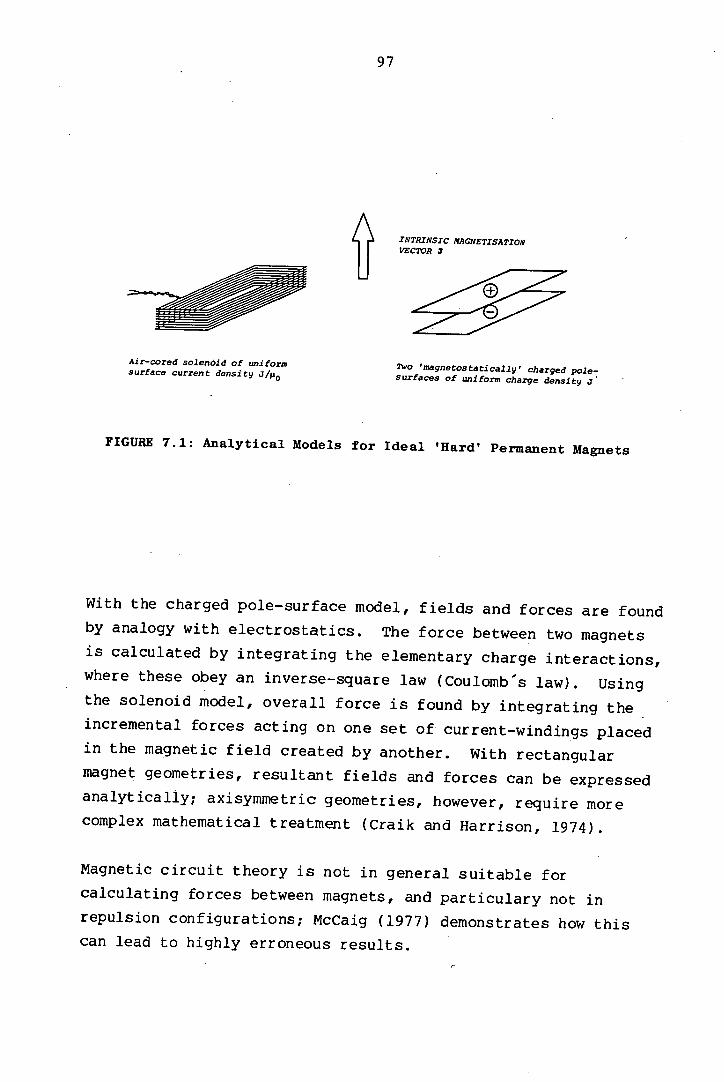
Air-cored solenOid of uniform surface current density
/o
INTRINSIC MAGNETISATION VECTOR
EE TWO magneeostatica1ly , charged pole-surfaces of uniform charge density .7
FIGURE 7.1: Analytical Models for Ideal 'Hard' Permanent Magnets
With the charged pole-surface model, fields and forces are found
by analogy with electrostatics. The force between two magnets
is calculated by integrating the elementary charge interactions,
where these obey an inverse-square law (Coulombs law). Using
the solenoid model, overall force is found by integrating the
incremental forces acting on one set of current-windings placed
in the magnetic field created by another. With rectangular
magnet geometries, resultant fields and forces can be expressed
analytically; axisymmetric geometries, however, require more complex mathematical treatment (Craik and Harrison, 1974).
Magnetic circuit theory is not in general suitable for
calculating forces between magnets, and particulary not in
repulsion configurations; McCaig (1977) demonstrates how this
can lead to highly erroneous results.

7.5 Optimising the Magnet Geometry
The geometry-optimisation analyses in this thesis are intended
to make it possible, having selected a particular bearing
characteristic, to find easily the magnet geometry which
provides this characteristic, using the minimum volume of
magnetic material. The bearing characteristic will ultimately
be specified in one of the following two ways:
As the minimum repulsion force required at a specified
value of magnet pole separation h (corresponding to the
lubricating film thickness), for example the equilibrium separation h e .
As the minimum stiffness required at a specified clearance.
Note that magnet dimensions optimised for maximum force are not
the same as those optimised for maximum stiffness (see section
8.6). In practice, the required repulsion force and stiffness
for the bearing will be specified in terms of local radial
magnetic pressure, and pressure increase per unit pole
deflection, respectively. The values will be local, rather than
applying to the bearing as a whole, on account of the compliance
of the magnet sheet: the overall stiffness of the bearing would
only be an appropriate criterion in a rigid-element design.
The above specification will be subject to one or more
constraints, with the result that any optimised geometry will
represent a mathematically 'local' rather than global
solution. The constraints are of the following forms:
(a) A stipulated minimum magnet cross-sectional size (see
figure 3.4). The magnets must be sufficiently large to ensure
that an acceptably small loss of repulsion force occurs under
the condition of maximum axial offset of opposing pole faces.
The possibility of some axial misalignment must be taken into account.
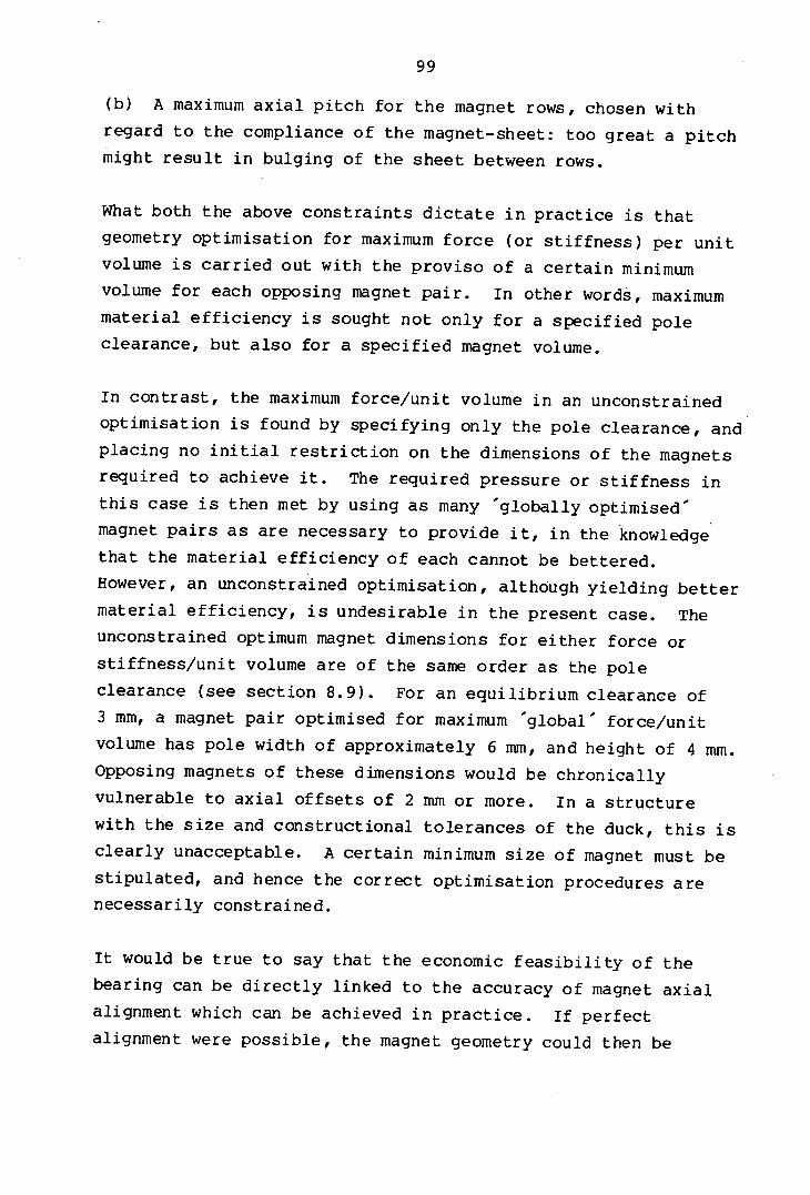
(b) A maximum axial pitch for the magnet rows, chosen with
regard to the compliance of the magnet-sheet: too great a pitch
might result in bulging of the sheet between rows.
What both the above constraints dictate in practice is that
geometry optimisation for maximum force (or stiffness) per unit
volume is carried out with the proviso of a certain minimum
volume for each opposing magnet pair. In other words, maximum
material efficiency is sought not only for a specified pole
clearance, but also for a specified magnet volume.
In contrast, the maximum force/unit volume in an unconstrained
optimisation is found by specifying only the pole clearance, and
placing no initial restriction on the dimensions of the magnets
required to achieve it. The required pressure or stiffness in
this case is then met by using as many 'globally optimised
magnet pairs as are necessary to provide it, in the knowledge
that the material efficiency of each cannot be bettered.
However, an unconstrained optimisation, althOugh yielding better
material efficiency, is undesirable in the present case. The
unconstrained optimum magnet dimensions for either force or
stiffness/unit volume are of the same order as the pole
clearance (see section 8.9). For an equilibrium clearance of
3 mm, a magnet pair optimised for maximum 'global' force/unit
volume has pole width of approximately 6 mm, and height of 4 mm.
Opposing magnets of these dimensions would be chronically
vulnerable to axial offsets of 2 mm or more. In a structure
with the size and constructional tolerances of the duck, this is
clearly unacceptable. A certain minimum size of magnet must be
stipulated, and hence the correct optimisation procedures are
necessarily constrained.
It would be true to say that the economic feasibility of the
bearing can be directly linked to the accuracy of magnet axial
alignment which can be achieved in practice. If perfect
alignment were possible, the magnet geometry could then be

100
optimised using an unconstrained technique, and blocks of small
cross-section (see above) used to make up the opposing rings.
Material efficiency would be very high. The greater the
maximum-likely misalignment, the larger the magnets need to be,
to provide a suitably large safety factor. A sophisticated and
expensive axial alignment system might actually result in an
overall reduction in bearing cost, by allowing the use of small opposing magnets.
7.6 Optimisation Procedures
The magnet pair cross-sectional dimensions are so much smaller
than the bearing radius (by a factor of 100) that bearing
curvature may be neglected. Furthermore, the effective length
of the equivalent linear magnet array is fixed as the
circumference of the bearing, and hence is not a variable. The
optimisation thus reduces to a two-dimensional one, in which the
quantities to be maximised are force and stiffness per unit
length, and these are sought by optimising the cross-sectional
dimensions of the magnet pairs. The fixed volume constraint for
a magnet pair (see above) reduces to a fixed-area constraint.
Further simplifications are made. By ignoring the
neighbouring-row interactions of the parallel rings in the
magnet array, only a single pair need be considered. If
sufficiently close axial pitching is adopted, neighbouring-row
interactions can actually increase total repulsion (see section
8.10): geometry optimisation in neglect of the effect thus
yields conservative estimates of required magnet volume. The
optimum geometry of an isolated pair can be used as the starting
point for more comprehensive (but more specific) analyses taking
account of neighbouring-row interactions (see Henning, 1973).
Only symmetric magnet-pairs, ie. with identical dimensions, are
considered. It can be mathematically demonstrated (see eg.
Coffey et al, 1972) that this is a prerequisite for any optimum
configuration, provided that there is no reason to minimise
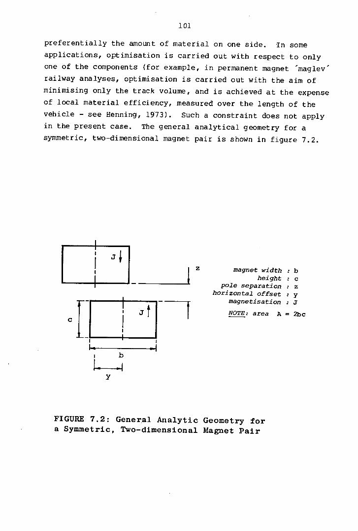
101
preferentially the amount of material on one side. In some
applications, optimisation is carried out with respect to only
one of the components (for example, in permanent magnet maglev
railway analyses, optimisation is carried out with the aim of
minimising only the track volume, and is achieved at the expense
of local material efficiency, measured over the length of the
vehicle - see Henning, 1973). Such a constraint does not apply
in the present case. The general analytical geometry for a
symmetric, two-dimensional magnet pair is shown in figure 7.2.
it
CI: ______
I
_______________________
s.I b
Y
Zmagnet width : b height : c
pole separation : Z
horizontal offset : y magnetisation : J
NOTE: area A = 2bc
FIGURE 7.2: General Analytic Geometry for a Symmetric, Two-dimensional Magnet Pair
102
With reference to figure 7.2, the most important optimisation
procedures carried out in the present study consist of:
Constrained maximum force/length: the vertical force/unit
length for a magnet pair of the given geometry is maximised for
a fixed total area A, where A = 2bc, over a range of values of
clearance z and lateral offset y. The optimum values of
pole-width b and height c are recorded in each case.
Constrained maximum stiffness/length: the vertical
stiffness/unit length is maximised in an exactly analogous procedure to (1) above.
Unconstrained maximum force/volume: for a given combination
of z and y the global optimum values of b and c are returned
which maximise force/volume (as force/unit length divided by
area A), with no constraint imposed on the total cross-sectional area.
Unconstrained maximum stiffness/volume: vertical
stiffness/unit volume for this geometry is maximised in the
analogous procedure to (3) above.
The last two analyses, although of limited usefulness in the
present application, are included for Completeness' sake: some
prior results exist in each case, though only for fully-aligned
magnets (y = 0), and based on graphical techniques, in contrast
to the present numerical analysis. Minnich (1971) and Coffey et
al (1972) both dealt with unconstrained force/volume procedures,
while Yonnet (1980) performed an unconstrained stiffness/volume
optimisation. The reason for including optimisation of
laterally-offset magnet pairs in the present analysis is to
allow such a contingency to be included in the bearing's force
or stiffness specification, ie. with an allowance for axial
misalignment incorporated in the economic optimum geometry.
103
The important differences between the optimisation analyses
described in the present work, and those previously published can be summarised thus:
The present analyses all invoke rigorous analytical and
numerical methods. The maxima of objective functions, eg.
force/unit volume, are found by numerically seeking zero values
of analytic function derivatives. Previous analyses have used
graphical estimates of curve maxima.
Constrained optimisation analyses of isolated magnet-pairs
do not appear to have been performed previously. The two most
important optimisation procedures with regard to the duck
bearing are those for maximum force/unit length and
stiffness/unit length, using a two-dimensional magnet pair of
fixed (constrained) cross-sectional area.
All the two-dimensional magnet optimisation schemes take
into account the possibility of horizontal pole-misalignment.
The case of fully aligned magnets (which was considered in
previous unconstrained optimisations) is thus special, rather than general, in the present study.
Two analyses of a three dimensional rectangular magnet pair,
again using rigorous optimisation techniques, are included for
interest. All theoretical results are presented in normalised
units, to allow them to be easily applied once the final force
and stiffness characteristics of the bearing are decided.
7.7 Related Work
The present analyses owe much to studies carried out in several
countries over the past twenty-five years, on applications of
permanent magnet repulsion as diverse as high-speed vehicle
levitation and small-scale frictionless bearings. In the former
category, the work of Baran (1962, 1964, 1971, 1972) and Henning
(1973) in Germany is especially noteworthy; Baran was one of the
104
first to perform rigorous performance analyses based on
pole-surface mathematics. Also recommended are the reports
prepared in the United States by Ford Motors (Borcherts, 1971),
the General Electric Company (Minnich, 1971), and Stanford
Research Institute (Coffey et al, 1972): the use of solenoid
mathematics was invoked in the first two of these. Small-scale
magnetic bearings have been comprehensively studied in France by
Yonnet (1978a, b, 1980, 1981a, b), who has identified the
procedures for optimising bearing geometry to yield maximum stiffness.
For an explanation of the fundamental properties of permanent
magnets, and the correct analytical techniques to use in field
and force calculations, the reader is encouraged to consult
McCaig (1977), whose work consistently emphasises the important
practical aspects of permanent magnet systems (1961, 1968). An
important experimental study is that of Tsui et al (1972).
Other works of related interest include a theoretical force/unit
volume optimisation of cylindrical magnets (Cooper et al, 1973),
and field calculations for rectangular magnet geometries (Craik, 1966, 1967).
7.8 Conclusions
The characteristics of ferrite magnets make them well suited for
use in the proposed bearing. Ferrites offer good magnetic
characteristics in repulsion applications, suffer from no corrosion problems, and are relatively cheap.
To calculate magnetic forces and stiffnesses, the magnets may be
represented either as charged pole surfaces or air-cored
solenoids. With rectangular magnet geometries, fully analytic
expressions for fields and forces can be obtained. The
magnet-pairs in the duck bearing can be represented as
symmetric, two-dimensional rectangular blocks. The important
geometry optimisation procedures in this study involve finding
the dimensions of an isolated magnet pair which maximise a
105
desired function, such as force/unit length, or stiffness/unit
volume. Two kinds of optimisation procedure are described. In
a constrained optimisation, the maximum material efficiency is
found assuming a fixed total volume of magnetic material, at a
particular pole clearance. In an unconstrained optimisation
procedure, only the magnet pole-separation is specified.
Because of the problem of magnet axial alignment, constrained
optimisation procedures are of more use in the present application.
The analyses described in the present work differ from those previously published, in that:
Computer-numerical methods are used to find function maxima
to greater accuracy than with prior graphical methods.
Constrained optimisation procedures are included.
Magnet horizontal offset is included as a variable.
The maximum likely axial offset of the bearing magnets is seen
as a fundamental factor in determining the overall cost of the
bearing. The better the alignment is, then the smaller, and more material efficient, can be the magnets.
106
CHAPTER 8
PERMANENT MAGNET OPTIMISATION
8.1 Chapter Summary
This chapter contains all the theoretical permanent-magnet
analyses performed in the present study. The expressions for
force/unit length and stiffness/unit length for a general
two-dimensional magnet pair are first given, after a brief
description of their derivation. Some typical theoretical
results are shown for magnets of a representative size, and the
scaling laws and normalisation procedures for force and stiffness are then listed.
Four optimisation analyses follow, all dealing with an isolated
two-dimensional magnet pair. The geometry is first optimised
with a constant-area constraint, for maximum force and
stiffness/unit length, and then with no constraint, for maximum
force and stiffness/unit volume. A worked example is included
to demonstrate how the results should be applied in practice. In a discussion of multiple-magnet arrays, the advantages of a
heteropolar configuration are explained, and theoretically
demonstrated. Finally, two analyses of a three-dimensional magnet pair are described.
8.2 Magnetic Forces
For the general case of a two-dimensional rectangular magnet
pair, force/unit length may be calculated using the analytical geometry illustrated in figure 8.1, in which one finite-length rectangular block is levitated above a second of infinite
length. Solenoid mathematics are used (see section 7.4), and in figure 8.1 the current windings are shown which are
mathematically equivalent to the real permanent magnet blocks.
The solenoidal current-density is given by J/ji0, where J is the magnetisation in tesla, and V O the universal magnetic constant, with value 471 x 10-7henrys/metre.
I.
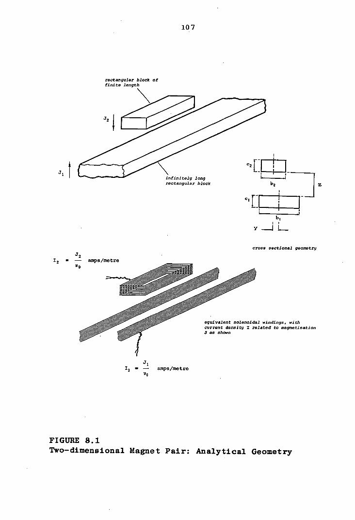
Ji f infinitely long rectangular block b2
C
-J
Y -_-I L. II
rectangular block of finite length
107
cross sectional geontry
1 2 - amps/metre p0
equivalent solenoidal windings, with current density I related to magnetisation .7 as shown
.1 1 amps/metre
NO
FIGURE 8.1 Two-dimensional Magnet Pair: Analytical Geometry
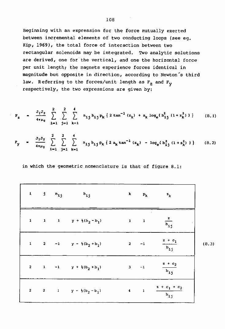
Beginning with an expression for the force mutually exerted
between incremental elements of two conducting loops (see eg.
Kip, 1969), the total force of interaction between two
rectangular solenoids may be integrated. Two analytic solutions
are derived, one for the vertical, and one the horizontal force
per unit length; the magnets experience forces identical in
magnitude but opposite in direction, according to Newtons third
law. Referring to the forces/unit length as F 2 and respectively, the two expressions are given by:
2 2 4 J 1 J2
Fz- - 4WLo
i=1 j=1 k=1
-1 2 2 njjbjjpk{ 2 tan (z k) +z1og{bjj(1+z)}} (8.1)
ly = 12
njjbjjPk{ 2 zktan ' (Zk) - loge b j (1+z) }}
0 i-i k=1
in which the geometric nomenclature is that of figure 81:
(8.2)
I j n1] b ij k Pk Z
1 1 1 y+½(b2 -b1 ) 1 1
Ij
1 2 -1 y - ½(b2 +b 1 ) Z + C1
2 -1 b ij
2 1 -1 y + ½(b 2 +b 1 ) Z + C2
3 -1 b ii
2 2 1 y - ½(b 2 -b 1 ) z + C1 + C2
4 1 b ij
(8.3)
109
From equations 8.1 and 8.2 it can be seen that force/unit length
is proportional to the magnetisation product J 1J2 , and hence in a system with like-magnets, proportional to J 2 . Force/unit volume is found as force/unit length divided by the total
cross-sectional area A where, from figure 8.1:
A = b1c1 + b2c2 (8.4)
From equations 8.1 and 8.2, the force/unit length can be found
for any two-dimensional magnet-pair. Some typical results are
shown in figure 8.2 for magnets with cross-sectional dimensions
and magnetic strength appropriate to the duck/spine bearing.
The three force-clearance curves correspond to fixed lateral
offsets of zero, one-quarter, and one-half pole-width. Note the
severe fall-off in vertical repulsion force with increasing
offset: at quarter pole-width offset, maximum repulsion force
falls to just over half its fully aligned value.
None of the curves behaves asymptotically as clearance tends to
zero, and a finite maximum force at pole-contact exists for
each. This may seem surprising: equation 8.1 can be derived
either from solenoid or coulomb-repulsion arguments (see section
7.4), and in both cases the incremental forces obey an •inverse
power law, ie. tending to infinity as clearance tends to zero.
However, this problem disappears on integration, and the
theoretical force at pole-contact is strictly calculable.
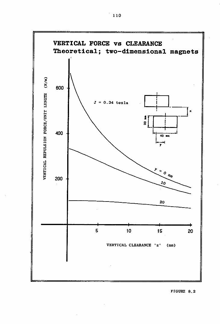
110
VERTICAL FORCE vs CLEARANCE Theoretical; two-dimensional magnets
p.' z
600
Z J = 0.34 tesla [
I-I z _J ifl___
o
E__ 44 400 1.1
40 mm z o 7
14
94 0 CA
0
200 .10
20
I I 5 10 IS 20
VERTICAL CLEARANCE 'z' (mm)
FIGURE 8.2
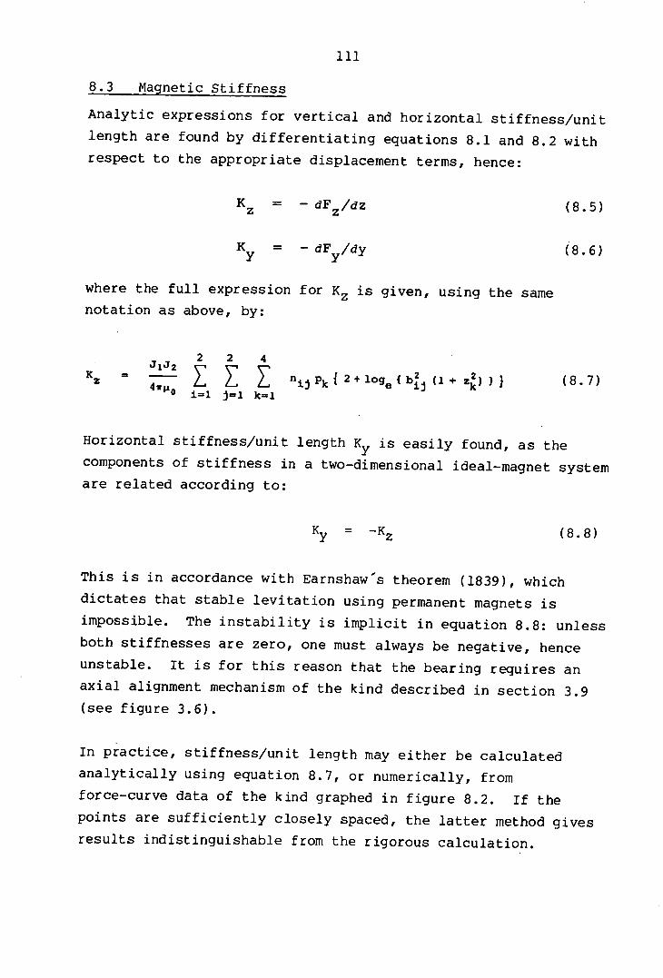
111
8.3 Magnetic Stiffness
Analytic expressions for vertical and horizontal stiffness/unit
length are found by differentiating equations 8.1 and 8.2 with
respect to the appropriate displacement terms, hence:
K z = — dF z /dz (8.5)
K -
= dF y v /dY (8.6)
where the full expression for K z is given, using the same notation as above, by:
2 2 4
K z -4w =
12 i Z Z 'ijk 1 2+log {b (1+ z) } } ( 8.7) IAO 1=1 j=1 k=1
Horizontal stiffness/unit length K is easily found, as the
components of stiffness in a two-dimensional ideal-magnet system are related according to:
K = Kz (8.8)
This is in accordance with Earnshaws theorem (1839), which
dictates that stable levitation using permanent magnets is
impossible. The instability is implicit in equation 8.8: unless
both stiffnesses are zero, one must always be negative, hence
unstable. It is for this reason that the bearing requires an
axial alignment mechanism of the kind described in section 3.9 (see figure 3.6).
In practice, stiffness/unit length may either be calculated analytically using equation 8.7, or numerically, from
force-curve data of the kind graphed in figure 8.2. If the
points are sufficiently closely spaced, the latter method gives
results indistinguishable from the rigorous calculation.

112
In figure 8.3 are shown the stiffness characteristics of the
same magnet-pair described in section 8.2 (see figure 8.2).
Note the highly nonlinear nature of vertical stiffness, and the
severe fall-off which occurs with non-zero lateral 'offset; the
effect is much more serious than that observed for force. With
zero lateral offset, vertical stiffness tends to infinity at
pole contact, in contrast to the behaviour observed for force.
This is one situation in which experiment and theory must
inevitably disagree.
8.4 The Scaling Laws for Force and Stiffness
The following four rules are general, and apply to all two- or
three-dimensional magnet arrangements:
Force is proportional to the square of scale.
Stiffness is directly proportional to scale.
Force/unit volume is inversely proportional to scale.
Stiffness/unit volume is inversely proportional to scale
squared.
In addition, the following two rules apply strictly to
two-dimensional geometries:
Force/unit length is directly proportional to the scale of
the cross-sectional dimensions.
Stiffness/unit length is independent of cross-sectional scale.
These laws are of great use in experimentally validating optimum
geometries (see sections 9.9 - 9.12). The importance of
observing geometric similarity is emphasised by McCaig (1961),
and as a corollary to the scaling laws, the following

/
113
VERTICAL STIFFNESS vs CLEARANCE
100 Theoretical; two-dimensional magnets
.
0 I-I
0 14
0
'4
4) f4-4 144
01
0
z . 40 MM
I- • 50
J = 0.34 tesla
Go
I I
5 10 15 20
VERTICAL CLEARANCE 'z' (mm)
FIGURE 8.3

114
procedures are noted for converting measured or calculated
quantities into scale-independent form, referring specifically
to the two-dimensional case:
Force/unit length is divided by a representative cross-sectional dimension.
Force/unit volume is multiplied by a representative cross-sectional dimension.
Stiffness/unit length is automatically scale-independent,
and needs no normalising factor.
Stiffness/unit volume is multiplied by the square of a
representative cross-sectional dimension.
Normalising is not the same as non-dimensionalising: all the
above quantities (a-d) have normalised units of N/m 2 , which follows from scaling law no.1. A normalised result is
equivalent to that which would accrue if the representative
dimension were unity, with all the other dimensions scaled in
proportion, according to geometric similarity.
8.5 Geometry Optimisation (1): Constrained Force/Unit Length
The aims of the four most important optimisation procedures were
described in section 7.6. In all cases the analytical geometry
is that shown in figure 7.2, ie. the two-dimensional case of
symmetric magnets with identical magnetisation. In the first
analysis, the maximum vertical force/unit length available from
a fixed total cross-sectional area A is found over a range of
values of pole-clearance z and lateral offset y, with the
optimum magnet width b and height c recorded in each case.
Although two optimum dimensions are required, there is only one

115
independent variable, as the constant-area constraint relates b and c according to:
C = A/2b (8.9)
where A is constant. Arbitrarily choosing b as the independent
variable, the maximum of the force/unit length function F2 for a given combination of z and y is found by setting:
dF2/db = 0 (8.10)
where:
dF2/db = F/ab + (3F2 /ac) dc/db
From equation 8.9:
dc/db = - c/b
(8.11)
hence, substituting 8.11 into 8.10, the required condition for a maximum of F 2 becomes:
aF/ab - c/b (F/ac) = 0 (8.12)
The partial derivatives 3F 2/ab and 9F2/ac are found analytically
by differentiating equation 8.1 with respect to the appropriate variables.
With a fixed area, the optimum geometry for a given combination
of z and y is then found solving equation 8.12, ie. by finding
the root of the nonlinear expression on the left hand side. A
solution corresponds to the optimum magnet width b0t under the particular conditions stipulated; the corresponding height copt
is then automatically found from equation 8.9.
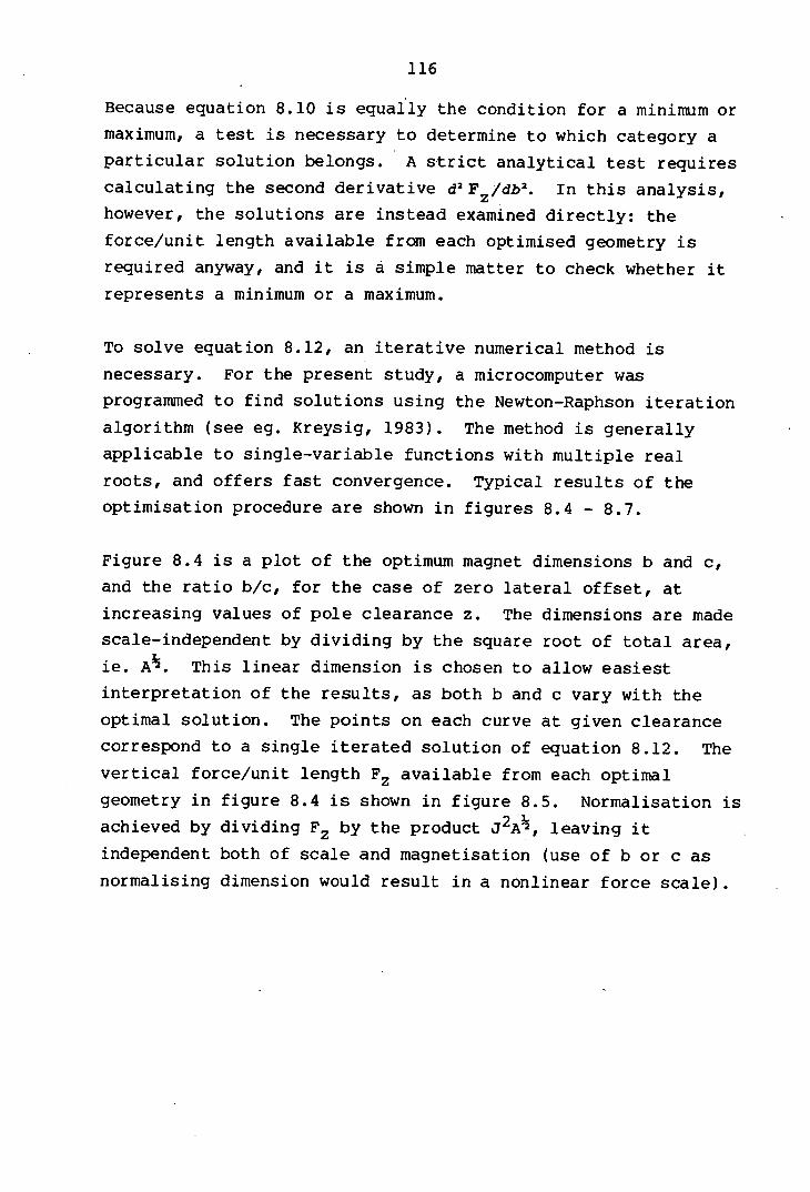
116
Because equation 8.10 is equally the condition for a minimum or
maximum, a test is necessary to determine to which category a
particular solution belongs. A strict analytical test requires
calculating the second derivative d2F/db2. In this analysis, however, the solutions are instead examined directly: the
force/unit length available from each optimised geometry is
required anyway, and it is a simple matter to check whether it
represents a minimum or a maximum.
To solve equation 8.12, an iterative numerical method is
necessary. For the present study, a microcomputer was
programmed to find solutions using the Newton-Raphson iteration
algorithm (see eg. Kreysig, 1983). The method is generally
applicable to single-variable functions with multiple real
roots, and offers fast convergence. Typical results of the
optimisation procedure are shown in figures 8.4 - 8.7.
Figure 8.4 is a plot of the optimum magnet dimensions b and c,
and the ratio b/c, for the case of zero lateral offset, at
increasing values of pole clearance Z. The dimensions are made
scale-independent by dividing by the square root of total area,
ie. A½. This linear dimension is chosen to allow easiest
interpretation of the results, as both b and c vary with the
optimal solution. The points on each curve at given clearance
correspond to a single iterated solution of equation 8.12. The
vertical force/unit length F z available from each optimal
geometry in figure 8.4 is shown in figure 8.5. Normalisation is
achieved by dividing Fz by the product J 2A½, leaving it
independent both of scale and magnetisation (use of b or c as
normalising dimension would result in a nonlinear force scale).

2 5 OPTIMUM MAGNET DIMENSIONS (1) For constrained maximum force/length
2.0 Z 1
lateral offset y/A½ = zero b/c c[I I
II I
• 7
- -
I .0 - b
-
0 0
c/As 0.5
0.2 0.4 0.6 0.8
CLEARANCE! (AREA)
FIGURE 8.4
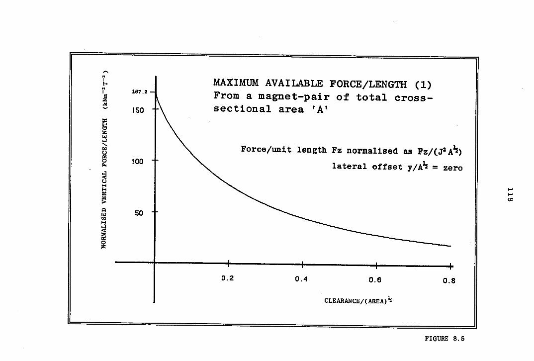
MAXIMUM AVAILABLE FORCE/LENGTH (1) 167.2- From 'a magnet-pair of total cross- ISO sectional area 'A'
Z
Force/unit length Fz normalised as Fz/(J 2 A2) 100
lateral offset y/A = zero
so
Q
Cl)
0.2 0.4 0.6 0.8
CLEARANCE/(AREA)
FIGURE 8.5

119
Figure 8.4 shows that, with increasing clearance between magnets
of fixed cross-sectional area, maximum repulsion force is
obtained by increasing the aspect ratio b/c. For two aligned
magnets making pole contact, the optimum ratio is given, to four
significant figures, by:
b/c0t = 0.9914 (8.13)
with the corresponding force/length found by:
Fz(opt) = 167.2 J2A½ kN/m (8.14)
Specific values of F(opt) are found using appropriate figures
for cross-sectional area A and magnetisation J in equation 8.14.
The above result, for zero clearance and zero offset, is an
important special case, as the value of Fz(opt) in equation 8.14
represents the maximum force/unit length which can ever be
achieved from a two-dimensional magnet-pair, in attraction or
repulsion. From equation 8.13, the optimum aspect ratio for
two-dimensional magnets making pole contact is seen to
correspond, to within 1%, to a square cross-section (b/c = 1).
Although a unity ratio might be more intellectually appealing,
the theoretical calculation appears to be correct, with the
optimum geometric ratio implicit in the following equation:
2 1 4R2 +4 tan- an' { }
= ; loge R + 4 (8.15)
R 3 + 3R
where R = b/c, and to which R = 1 is not a solution.
In figures 8.6 and 8.7, the results are shown for an
optimisation scheme identical to the above, but with non-zero
lateral offset; in this case y/A = 0.2. At pole contact,
Fz (OPt) is now some 23% less than in the fully-aligned case,
despite the relatively small offset. The corresponding optimum
dimensional ratio b/c is not, however, greatly different.
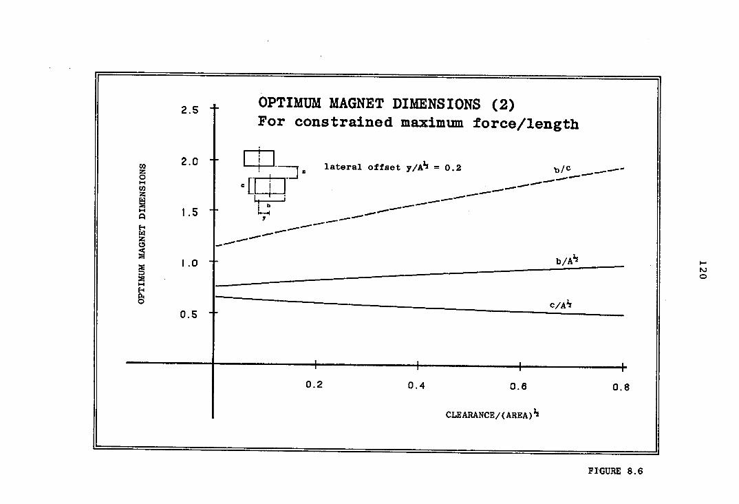
Co z 0
Cl) z
z
0
2.5 t MAGNET DIMENSIONS (2)
I For constrained maximum force/length
20 lateral offset y/A½= 0.2 b/ c ....-._ - - - - - - - -
I t
1.0 T b/A½
b 15
-
c/As 0.5
0.2 0.4 0.6 0.8
CLEARANCE/(AREA)½
0
FIGURE 8.6
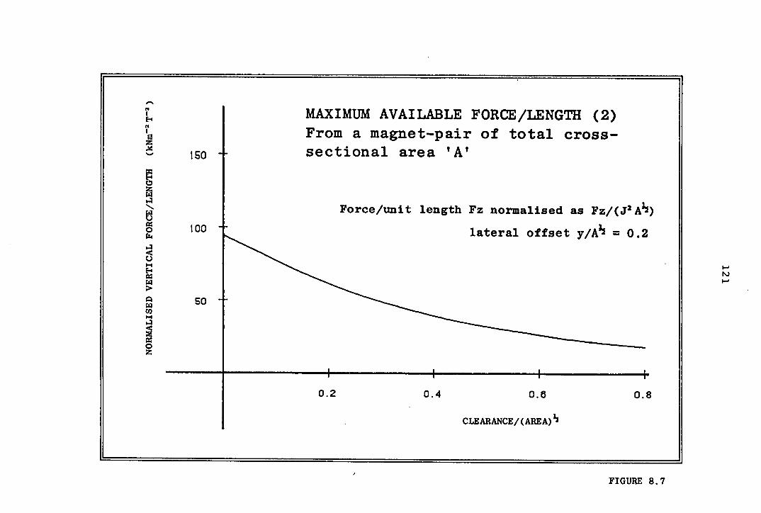
z
0 r14
C.) '-I
U)
I MAXIMUM AVAILABLE FORCE/LENGTH (2)
I From a magnet-pair of total cross- so 4 sectional area TAT
I Force/unit length Fz normalised as Fz/(J 2 A½)
tOO lateral offset y/A = 0.2
50
0.2 0.4 0.6 0.8
CLEARANCE! (AREA)
I'J
FIGURE 8.7
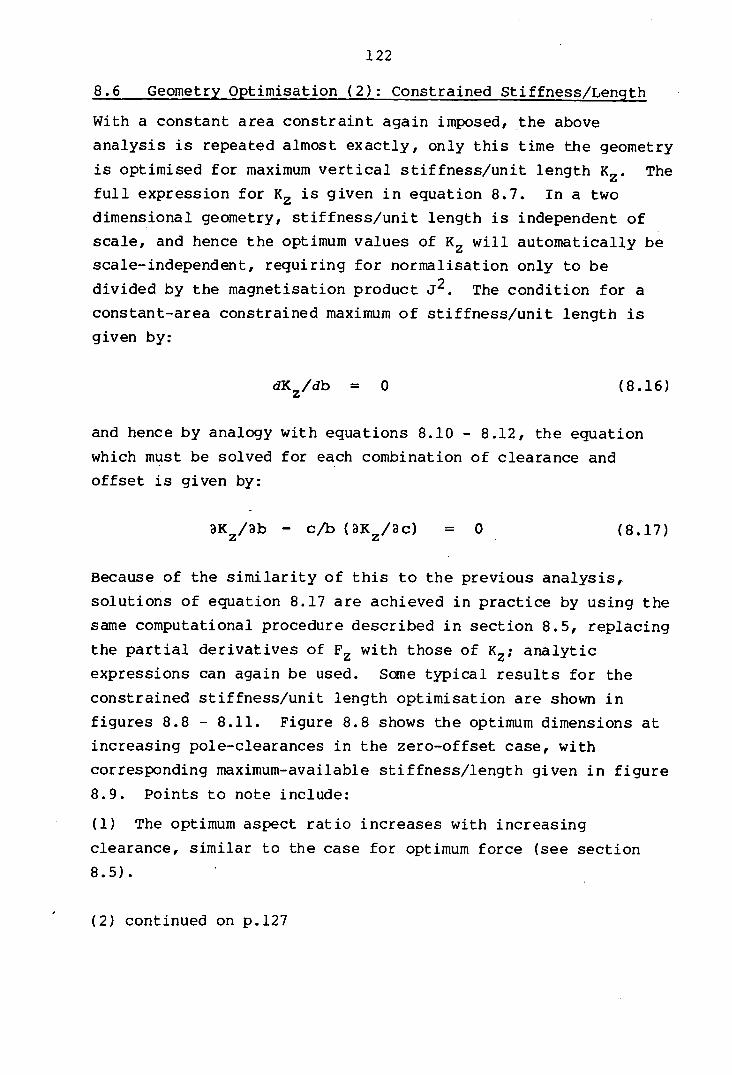
122
8.6 Geometry Optimisation (2): Constrained Stiffness/Length
With a constant area constraint again imposed, the above
analysis is repeated almost exactly, only this time the geometry
is optimised for maximum vertical-stiffness/unit length K 2 . The full expression for K2 is given in equation 8.7. In a two dimensional geometry, stiffness/unit length is independent of
scale, and hence the optimum values of K 2 will automatically be scale-independent, requiring for normalisation only to be
divided by the magnetisation product J 2 . The condition for a
constant-area constrained maximum of stiffness/unit length is
given by:
dK/db = 0 (8.16)
and hence by analogy with equations 8.10 - 8.12, the equation
which must be solved for each combination of clearance and
offset is given by:
3K2/ab - c/b (3K/3c) = 0 (8.17)
Because of the similarity of this to the previous analysis,
solutions of equation 8.17 are achieved in practice by using the
same computational procedure described in section 8.5, replacing
the partial derivatives of F 2 with those of K; analytic expressions can again be used. Some typical results for the
constrained stiffness/unit length optimisation are shown in
figures 8.8 - 8.11. Figure 8.8 shows the optimum dimensions at
increasing pole-clearances in the zero-offset case, with
corresponding maximum-available stiffness/length given in figure
8.9. Points to note include:
(1) The optimum aspect ratio increases with increasing
clearance, similar to the case for optimum force (see section
8.5).
(2) continued on p.127

Z 0
2 OPTIMUM MAGNET DIMENSIONS (1) For constrained maximum stiffness/length
I I. -. lateral offset y/A½ = zero b/c .....
[.1 I,
b
7
1.0
06515—.
0.2 0.4 0.6
0.8
(A)
CLEARANCE/(AREA)
FIGURE 8.8
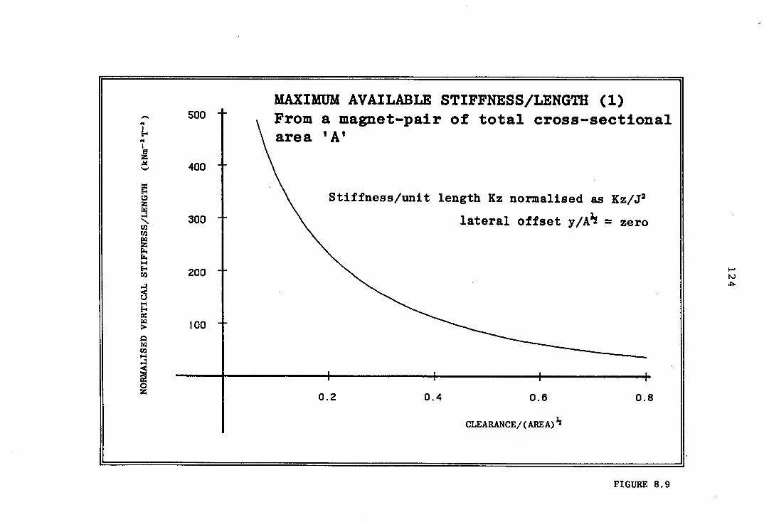
MAXIMUM AVAILABLE STIFFNESS/LENGTH (1) 500 Erom a magnet-pair of total cross-sectional
I \ area 'A'
N U) CI)
r4 r4
U)
I
400
I \ Stiffness/unit length Kz normalised as Kz/J 2
oo lateral offset y/A½ = zero
200
0.2 0.4 0.6
0.8
CLEARANCE/(AREA)½
.4 'S
'-a
FIGURE 8.9
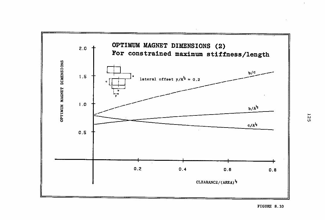
2 0 t OPTIMUM MAGNET DIMENSIONS (2) For constrained maximum stiffness/length
lateral offset y/A½ = 0.2 — — - C
b
z f: 1.0 -.—
b
0
0.5*
0.2 0.4 0.6 0.8
t'J U,
CLEARANCE! (AREA)
FIGURE 8.10

500 MAXIMUM AVAILABLE STIFFNESS/LENGTh. (2) From a magnet-pair of total cross-sectional
400
area 'A'
300 Stiffness/unit length Kz normalised as Kz/J 2
PW
lateral offset y/A½ = 0.2
200 I-.
100
2O.4 0.6 Q.8
CLEARANCE/(AREA)½
FIGURE 8.11
127
Although maximum-available stiffness tends to infinity as
clearance tends to zero, the optimum aspect ratio at pole
contact remains well-defined, with:
b/c0t = 0.6515
(8.18)
Magnet geometries optimised for stiffness have different
dimensions to those optimised for force: compare solutions 8.18
and 8.13, where both represent optimum pole-contact geometries.
The optimum geometry given by equation 8.18 is an approximation:
for this special case, it can be rigorously shown that:
= b/c opt +
(8.19) 9/97
Figures 8.10 and 8.11 illustrate the results of a similar
analysis, in which a non-zero lateral offset is specified. In
this case, the maximum-available stiffness tends to a finite
limit as the pole-clearance approaches zero.
8.7 Optimisation: Applying the Results
To illustrate how the above constrained-optimisation schemes are
used in the context of the duck bearing, consider the following
example. Suppose that, on stipulating a certain axial magnet
pitch, the bearing pressure specification translates into the
following requirement: at the minimum allowed pole separation, a
single magnet pair must provide a repulsion force of 1000 N per
metre circumferential length, but comprise no more than 20
kg/metre of magnet material; strontium ferrite magnets are to be used.
The desired parameters are the maximum pole-clearance possible
within the above constraints, and the optimum magnet dimensions
which allow it.
128
Taking the density of strontium ferrite as 4800 kg/m3 , the
weight constraint corresponds to a maximum magnet volume of
4.167 x io m3 per metre of magnet length, and hence a total
cross sectional area A of 4.167 x 10 -3 m2 . The force/length
requirement is 1000 N/rn: to express this in normalised units,
divide by 3 2A½, where J is typically 0.32 tesla; the resulting
normalised force/length F z equals 151.3 kNm 2T 2 . Using the
curve in figure 8.5 (or, better, a computer-generated look-up
table) the dimensionless clearance corresponding to
F(normalised) is given by z/A½ = 0.0146, which represents a
true clearance of 0.94 mm. From figure 8.4 the optimum magnet
aspect ratio is read off against dimensionless clearance, hence
= 1.01.
The resulting optimised system dimensions would thus be:
cross sectional area A/2, single magnet = 2084 mm 2
optimum magnet aspect ratio b/c = 1.01
hence magnet-width b = 45.8 mm (8.20)
height c = 45.5 mm
maximum pole-separation z = 0.94 mm
The results of the stiffness optimisation scheme of section 8.6
would be applied in exactly the same way as above, had the
initial specification been expressed in terms of required
stiffness rather than force per unit length.
In general terms, what the results of the two preceding analyses
allow is stipulation of any two parameters from a choice of
force (or stiffness), magnet-weight, and pole clearance, with
the optimum value of the third then returned, together with the
appropriate magnet dimensions.
129
8.8 Geometry Optimisation (3): Unconstrained Force/Unit Volume
In this, and the subsequent, optimisation procedure, no
constraint is placed on magnet cross-sectional area, and for any
given combination of clearance and offset, the maximum value of
force or stiffness per unit volume is found by seeking the
global-optimum-magnet dimensions.
The analytical.geometry is again that shown in figure 7.2. In
the first case optimisation is for maximum vertical force/unit
volume Fyi where for symmetric magnets:
Fv = Fz/2bC
(8.21)
where Fz is given by equation 8.1. Imposing no constraint on
area, the magnets' width and height are independent variables,
and a global maximum of Fv is found from:
aF/ab = aF/ac = 0
(8.22)
which, from equation 8.21, then represents the simultaneous
requirements:
aF/ab - F/b = 0 (8.23)
- Fe /C = 0 (8.24)
The partial derivatives are the same as previously used in the
constrained optimisation procedure. In this case however, a
more sophisticated optimisation algorithm is necessary: there
are now two conditions to be simultaneously satisfied, where
before, a function of only one variable was involved. The
algorithm used in the present study was the method of steepest
ascent', an optimisation technique suggested by Box et al (1969)
which is applicable to nonlinear functions of many variables,
and in which an iterative search is used to find simultaneously
the values of all the variables corresponding to a maximum of

130
the objective function (in this case F), with a solution
returned when all the partial derivatives equal zero. The
routine was again implemented on a microcomputer.
For a given combination of pole-clearance and offset, the
solution to equations 8.23 and 8.24 consists of the maximum
available force/unit volume Fv(opt), and the corresponding
values of magnet dimensions b and c. Once the optimum solution
is known for a given ratio y/z, the solutions for this ratio at
any scale are automatically known, using the laws given in
section 8.4. Consequently, the results of the present
optimisation scheme, expressed in normalised units of F(opt),
form a single curve, plotted against the dimensionless ratio
y/z. This curve is shown in figure 8.12, while figure 8.13
gives the corresponding optimum magnet dimensions.
The values of F(opt) are normalised according to section
8.4(b): the use of pole clearance as the normalising
cross-sectional dimension allows the curves to be interpreted as
results predicted for increasing offset at constant clearance.
It is then seen that maximum available force/unit volume
decreases with offset, while increasingly large magnets are
required to achieve optimum material efficiency (as demonstrated
by an increase in both width and height, ie. b/z and c/z
respectively). However, the optimum aspect ratio b/c remains
roughly the same over the range y/z = 0 to 2. For the case of
fully aligned magnets (y/z = 0), the results are directly
comparable with those of Minnich (1971) and Coffey et al (1972),
in whose analyses force maxima were estimated graphically. In
both cases the optimum dimensional ratios were estimated as
b/z = 2.0 and c/z = 1.5, compared with the present results:
b/z0t = 2.005 (8.25)
C/Zopt = 1.372 (8.26)

131
MAXIMUM POSSIBLE FORCE/VOLUME At rr4 tT? i1 ,. t
FIGURE 8.12
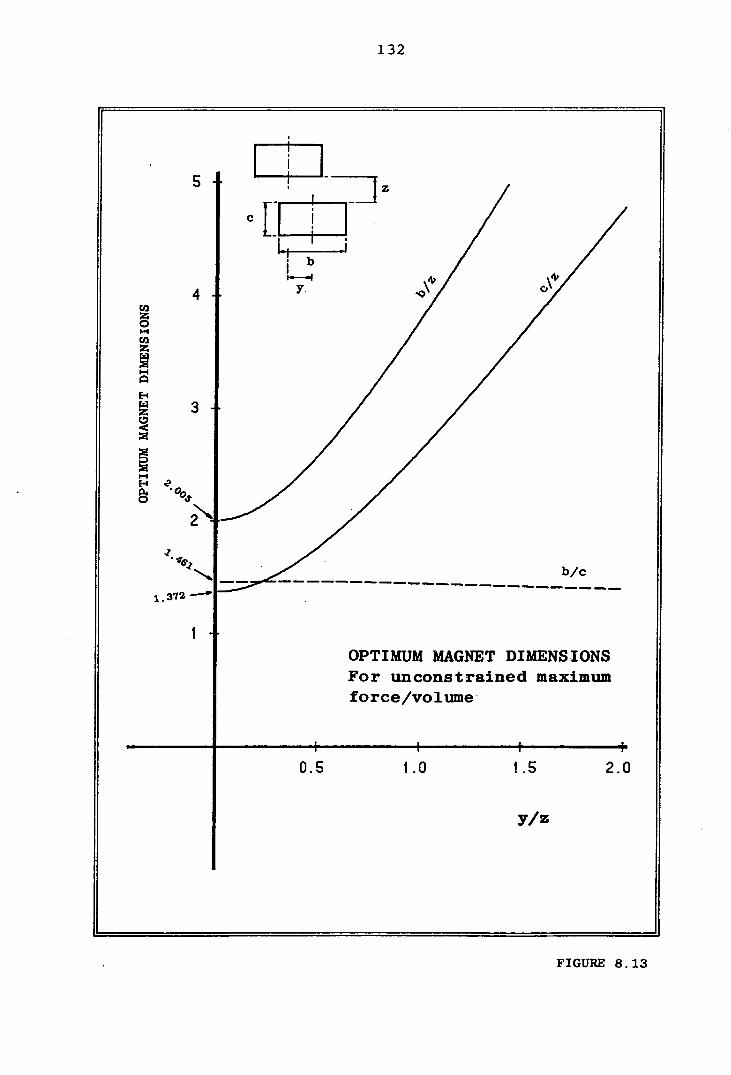
132
1/ 'F
16' b/c
372
OPTIMUM MAGNET DIMENSIONS For unconstrained maximum force/volume
I I I 0.5 1.0 1.5 2.0
y/z
FIGURE 8.13
133
The maximum-possible force/unit volume is given, from the
present analysis, by:
Fv(Opt) = 18.12 J2/z kN/m3 (8.27)
with the force/unit length of the optimum geometry found from:
Fz (opt) = 99.74 Jz kN/m (8.28)
Although the present results predict a magnet height c/z0 t some
8.5% smaller than the previous estimates, the above value of
maximum force/unit volume is only 0.2% higher than that
calculated on the basis of the previous graphically-found
dimensions, indicating that Fv (OPt) is relatively insensitive to magnet-height in the region of the optimum geometry. This
highlights a strength of the present analysis, showing the
numerical method to be more suited to pinpointing a relatively
flat maximum. However, it is noteworthy that in terms of
material efficiency there is little to choose between the
optimum magnet dimensions predicted here, and those previously
published.
8.9 Geometry Optimisation (4): Unconstrained Stiffness/Volume
The procedure in this case is exactly equivalent to that in
section 8.8, though with the objective function now
stiffness/unit volume Ky rather than force/unit volume Fv . Hence, by analogy with equations 8.23 and 8.24, the simultaneous
requirements for a global maximum of K v are given by:
aK2/m - Kg/b = 0 (8.29)
aK/ac - Ks/c = 0 (8.30)
where the partial derivatives are evaluated, as before, from
equation 8.7. Solutions to equations 8.29 and 8.30 are found
using the gradient-search technique described in section 8.8.
134
Normalisation of K(opt) is achieved by multiplying by z 2/J2
(see section 8.4): choice of the clearance z as the normalising
dimension is explained in section 8.8.
The results of the analysis are presented in figures 8.14 and
8.15. Figure 8.14 shows that K(opt) decreases very sharply
(note the log scale) with offset. For the case of zero lateral
offset the 'maximum stiffness/volume is given by:
Kv(opt) = 23.45 J2/z2 kN/m per cubic metre (8.31)
The optimum magnet dimensions corresponding to this case are:
= 1.018
= 0.6697 (8.32)
b/Cot = 1.519
The special case of fully-centred magnets was previously
considered by Yonnet (1980) who, from graphical solutions, found
the value of c/z0t to lie between 0.5 and 1.0, with
corresponding b/Zopt of approximately 1; his figure for K v (opt) was 23 J2/z 2 kN/m/m3 , a value very close to that of the present
numerical analysis. In a similar manner to the dependence of
maximum force/unit volume on magnet height, discussed in section
8.8, the above figure for K(opt) is relatively insensitive to
the same parameter: this is demonstrated in the high accuracy of
Yonnets maximum stiffness estimate, calculated on the basis of
approximate optimum magnet dimensions.
For increasing lateral offset (as the ratio y/z), the maximum
available stiffness/unit volume decreases in a similar manner to
that observed with force/unit volume, with larger magnets again
required to achieve optimum material efficiency. It is
important to remember that any two-dimensional magnet system

135
MAXIMUM POSSIBLE STIFFNESS/VOLUME At e,1 . I ria4
FIGURE 8.14
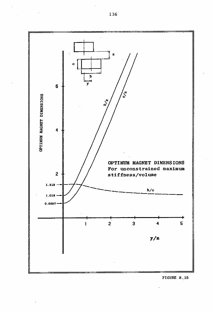
136
II / I
6 1/
pq
I i I\
z I IC' 0
OPTIMUM MAGNET DIMENSIONS For unconstrained maximum
2 stiffness/volume
1.519 -
- b/c 1.018
O.6697-
I . I 2 3 4 5
y/z
FIGURE 8.15
137
optimised for maximum vertical stiffness is automatically
optimised for maximum horizontal (negative) stiffness as well,
and hence for maximum lateral instability: this is a consequence
of Earnshaws theorem (see section 8.3).
It can be seen that an unconstrained geometry optimisation is
unsuitable in the case of the duck bearing. Assuming an
equilibrium pole clearance of 3 mm, and optimising firstly for
maximum force/unit volume, the appropriate pole-width b is found
from equation 8.25 to be approximately 6 mm. Optimising instead
for stiffness/unit volume, equation 8.32 gives the required
pole-width as approximately 3 mm. In either case, the magnet
dimensions are of the same order as the lateral offsets likely
in normal operation, and would result in a system liable to
complete collapse (or reversal - see section 8.10) of repulsion
force.
8.10 Multiple-Pair Magnet Arrangements
The above optimisation procedures are all based on a single
magnet-pair interaction. In practice, each magnet on one side
of the proposed bearing clearance (see figure 3.4) experiences a
force of interaction with every magnet on the other side.
Although the axial pitch of the bearing magnets will probably be
too great to make this a significant effect, it will nonetheless
enhance the repulsion pressure to some extent. In economic
terms, optimum geometries based on the preceding results will
thus be conservative; the appropriate method for calculating the
true characteristics of a given arrangement. is described below.
The total vertical force exerted in a multiple-row system is
calculated by superposition of single-pair interactions. In a
system of n parallel rows, the total repulsion force comprises
n2 components, where each corresponds to a single-pair
interaction: these can be calculated from equation 8.1. For
systems of identical opposing-magnet geometry and uniform
lateral pitch, it is, however, unnecessary to perform n2

138
calculations to find the resultant force. Because of inherent
symmetry, many of the individual-pair interactions. are
duplicated (at least in magnitude, if not direction) and it can
be shown that the maximum number of calculations necessary in an
arrangement of the present kind is only 2n-1.
Previous analyses of two-dimensional multiple-pair
configurations have reduced the number of calculations still
further. Both Minnich (1971) and Henning (1973) introduced a
lateral zone of influence' to either side of a given magnet,
with only those interactions lying within the zone counting
towards the total force, the others being sufficiently weak to
neglect. This not only greatly reduced the number of
calculations necessary, but dispensed with the need to calculate
very small forces as the difference between large ones, which
situation arises with widely-separated magnets.
To demonstrate the increase in repulsion arising from
cross-interactions, the results shown in figures 8.16 - 8.18
were calculated for a 9-row system, with opposing magnet-pairs
of the same dimensions as those considered in sections 8.2 and
8.3 (see figures 8.2 and 8.3), and a lateral pitch of 60 ian.
Note that adjacent rows present alternating polarity, in the
so-called 'heteropolar' configuration: perhaps contrary to
intuition, this arrangement is necessary if the first (and
strongest) cross-interaction is to be a repulsion, rather than
an attraction. The overall repulsion in a homopolar
configuration is by the same token weaker than the sum of its
component interactions (see Baran, 1971).
In figure 8.16, the benefit accruing from a close-pitched
heteropolar layout is seen: overall repulsion is compared with
that calculated as nine times the single-pair interaction force.
The corresponding increase in stiffness is shown in figure 8.17.
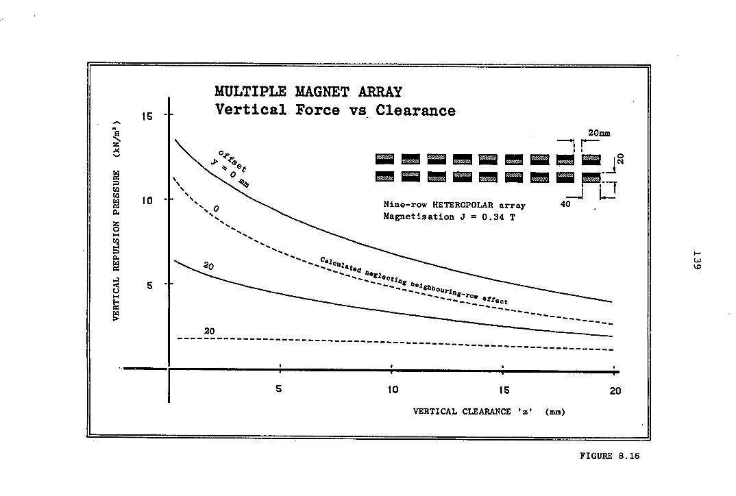
MULTIPLE MAGNET ARRAY Vertical Force vs Clearance -
20mm
N
—JLi 10 Nine-row HETEROPOLAR array 40
Magnetisation J = 0.34 T z 0
_row Oct 20
5 10 15 20
VERTICAL CLEARANCE 'z' (mm)
I-.
'0
FIGURE 8.16
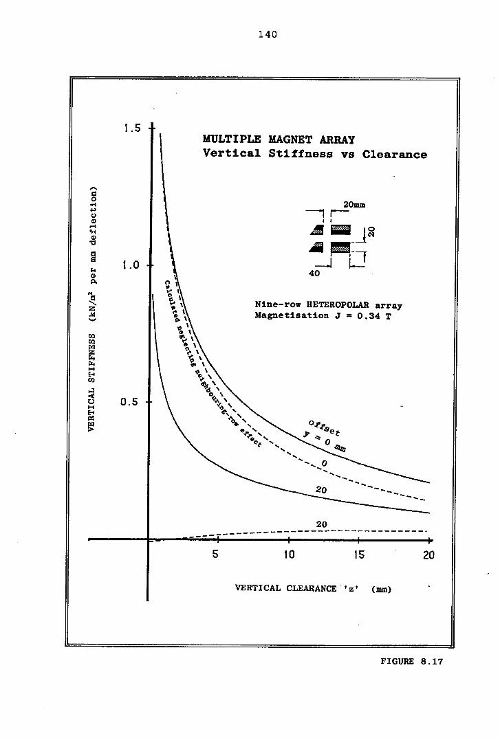
1 .5 MULTIPLE MAGNET ARRAY Vertical Stiffness vs Clearance
0
C)
I-I CH G)
1.0
':1) Cl) rx z rx-
94
Cl)
C.) 0.5
0
Nine-row HETEROPOLAR array Magnetisation J = 0.34 T
set
p.' ',e \
0%
vs 05
20 - - -
20 I
I-
5 10 15 20
VERTICAL CLEARANCE 'z' (mm)
140
FIGURE 8.17
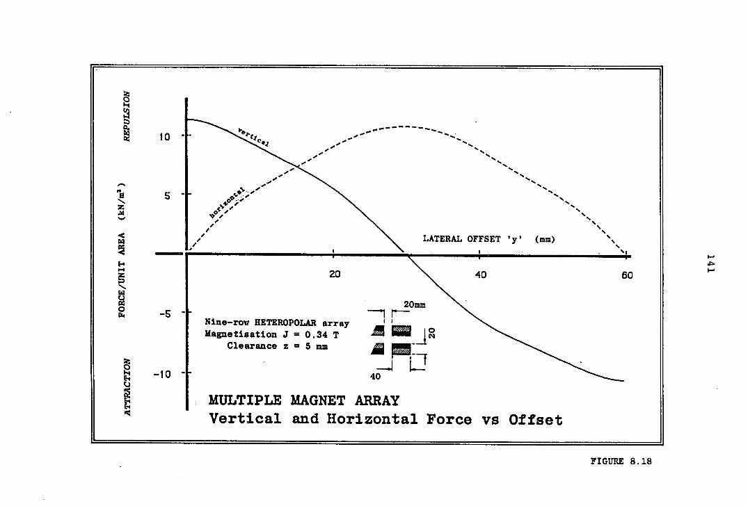
II
a Z
EI
S
-
.-.'
.'%
.'%
..'
S. S.
.' S.
S. S.
S. S.
LATERAL OFFSET 'y' (mm)
20 40 N.
20= 44 -5
Nine-row HETEROPOLAR array Magnetisation J = 0.34 T -
Clearance a 5 mm 1/14
0
I •0
MULTIPLE MAGNET ARRAY Vertical and Horizontal Force vs Offset
FIGURE 8.18
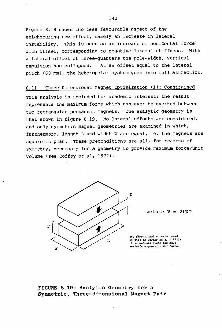
142
Figure 8.18 shows the less favourable aspect of the
neighbouring-row effect, namely an increase in lateral
instability. This is seen as an increase of horizontal force
with offset, corresponding to negative lateral stiffness. With
a lateral offset of three-quarters the pole-width, vertical
repulsion has collapsed. At an offset equal to the lateral
pitch (60 mm), the heteropolar system goes into full attraction.
8.11 Three-Dimensional Magnet Optimisation (1): Constrained
This analysis is included for academic interest: the result
represents the maximum force which can ever be exerted between
two rectangular permanent magnets. The analytic geometry is
that shown in figure 8.19. No lateral offsets are considered,
and only symmetric magnet geometries are examined in which,
furthermore, length L and width W are equal, ie. the magnets are
square in plan. These preconditions are all, for reasons of
symmetry, necessary for a geometry to provide maximum force/unit
volume (see Coffey et al, 1972).
Tj
volume V = 2LWT
The dimensional notation used is that of Coffey et al (1972); these authors quote the full analytic expression for force.
VV
FIGURE 8.19: Analytic Geometry for a Symmetric, Three-dimensional Magnet Pair
143
The three-dimensional magnet geometry is analysed to find the
following two quantities:
The maximum vertical repulsion force F available from a
fixed total volume V.
The maximum-available vertical force/unit volume F/v at any
clearance z (see section 8.12).
The first of these requires a constrained optimisation with
fixed total volume V where, for the given geometry:
V = 2W2T (8.33)
From which:
W = (v/2T)½ (8.34)
Imposing a constant-volume constraint reduces the repulsion
force F to a function of only one variable: thickness T is
arbitrarily chosen. Maximum force occurs at pole-contact, and
hence the required condition for a maximum is given by:
dF/dTø = 0 (8.35)
From equation 8.33,the expression for a constant-volume
constrained maximum is then:
3F/DT + (aF/aw) aW/dT = 0 (8.36)
and hence, from 8.34 and 8.36, the required condition for a
constrained maximum is:
3F/3T - W/2T (aF/aW) = 0 (8.37)

144
An expression for repulsion force F for the geometry in figure
8.19 is presented by Coffey et al (1972); for the optimum
solution, this reduces to the case where L = W (see above). The
appropriate partial derivatives are calculable in fully analytic
form, from which the solution to equation 8.37 may be found
using the Newton-Raphson root-seeking algorithm previously
employed in two-dimensional constrained optimisations (see eg.
section 8.5). The resulting optimum dimensions are:
width Wopt = 1.072 V 1"3
thickness T0t = 0.4548 V"3 (8.38)
W/Topt = 2.466
The corresponding maximum-available force is given by:
Fopt = 237.9 J20"3 kN (8.39)
This last figure represents the maximum force which can ever be
exerted by two rectangular bar magnets.
8.12 Three-Dimensional Magnet Optimisation (2): Unconstrained
Finally, the maximum-possible force/unit volume is found for a
three-dimensional magnet-pair. The analytic geometry is the
same as in section 8.11, ie. symmetric, square magnets. This
time, however, there is no constant-volume constraint, and
simultaneous solutions are required to the following two
equations:
3/9T (F/V) = 0 (8.40)
a/aw (Fly) = 0 (8.41)
145
Using the relationship given by equation 8.33, the above
requirements are expressed as:
(3F/aT - F/T) = 0 (8.42)
(3F/aW - 2F/w) = 0 (8.43)
To obtain simultaneous solutions to equations 8.42 and 8.43, the
method of steepest-ascent (described in section 8.8) is used.
In the present case the objective function is F/V, and the two
independent variables are the magnet dimensions W and T;
clearance z is. constant. The analysis yields the following
results:
= 3.079
T/Zopt = 1.357
(8.44)
W/Topt = 2.269
with the corresponding maximum-available force/unit volume given
as:
= 20.40 J2/z kN/m3
(8.45)
The above value of. F/Vot can be directly compared with that for
a two-dimensional magnet-pair, given in equation 8.27. The
optimised three-dimensional magnets are then seen to represent
12.5% more efficient use of magnetic material.
In their analysis of this geometry, Coffey et al (1972) found
the optimum magnet dimensions graphically, with resulting values
for W/z0t and T/Zopt of 3.0 and 1.5, repectively, and
corresponding F/Vopt of 20,300 J 2 /z N/rn 3 . As in the
two-dimensional case, a relatively wide latitude is seen to
exist in the magnet dimensions capable of delivering
146
near-optimum efficiency. These authors' results indicate a
value of maximum force/unit volume only 0.5% less than that of
the present analysis, although using magnets with a total volume
some 8% greater.
8.13 Conclusions
The geometry optimisation schemes described in this chapter make
possible the following procedures, referring to a
two-dimensional magnet pair:
By specifying any two parameters from a choice of
force/unit length, magnet-weight, and pole-clearance, the
optimum value of the third can be automatically found. This
includes cases where a horizontal pole-offset is assumed.
As in (1) above, replacing force/unit length with
stiffness/unit length.
By specifying pole clearance alone, the maximum force/unit
volume or stiffness/unit volume can be found. Again, lateral
offsets may be stipulated.
The way in which an optimum magnet geometry might be selected in
practice has been demonstrated in a worked example. Several of
the results of both the two-dimensional and the
three-dimensional geometry optimisation analyses represent
special cases, in which the material efficiency represents the
maximum which can be achieved using hard magnets. These results
are summarised in table 8.1. In some instances previous
estimates exist for optimum dimensions (see table 8.1), and the
results of the present study are found to differ from these by
up to about 9%. The new estimates should be the more accurate,
on account of the computer numerical methods used to estimate
function maxima. The optimisation results are highly general,
and apply to any system for which ideal-magnet assumptions can
be made.

TABLE 8. 1 TWO-DIMENSIONAL THREE-DIMENSIONAL
Summary of 'special case' optimum rectangular magnet geometries. Those marked with an asterisk (*) have [ 4 1
magnet width : b height : C
previously been estimated by 1 separation z magnetisation :
- magnet width : W
semi-graphical techniques. l ength L height : T
For details of the analyses, C NOTE: area A T
pole separation
refer to the sections noted ________
magnetisation : J
In each case. b NOTE volume V 21WT -
Maximum vertical repulsion force available Force F 237.9 j2v2/3 kN from a rectangular magnet pair of combined Force/unit length F5 167.2 J2A kN/in
volume V (three-dimensional case) or cross sectional area A (two-dimensional case). Optimum aspect ratio b/c 0.9914 Optimum dimensional ratios: W/T 2.466 Pole contact (z 0) is assumed. L/T
(see section 8.5) (see section 8.11)
Maximum force/unit volume available from a * rectangular magnet pair at a given pole Force/unit volume F18.12 J2 /z kN/m3 Force/unit volume F/v 20.40 J2/Z kN/m3 clearance z.
v
Optimum dimensions: b - 2.005 z Optimum dimensions: W 3.079 z
C l.372z (see section 8.8)
L = T
(see section 8.12)
Maximum vertical stiffness available from a rectangular magnet pair of combined volume Stiffness/unit length K is theoretically z N/A V (three-dimensional case) or cross sectional infinite. area A (two dimensional case). Pole contact (z 0) is assumed. Optimum aspect ratio b/c = 0.6515
(see section 8.6)
Maximum stiffness/unit volume available from S.
Stiffness/unit volume K= 23.45 J2 /z2 a rectangular magnet pair at a given pole v kN/m" N/A
clearance z. Optimum dimensions: b 1.018 z
c 0.6697 z (see section 8.9)
I-
148
In terms of the present application, the increase in repulsion
which can be gained by using a close-pitched heteropolar magnet
array has been demonstrated. So too has the danger of axial
misalignment of opposing magnets in the bearing. As a rough
guide, the maximum lateral offset of opposing pole faces should
not exceed about 20% of their width. This highlights the
relationship which exists between axial alignment and bearing
cost: the better the alignment possible, the smaller the magnets
which can be used.
149
CHAPTER 9
PERMANENT MAGNET ANALYSIS - EXPERIMENTAL RESULTS
9.1 Chapter Summary
The experiments described in this chapter were designed to
verify the results of the optimisation procedures contained in
chapter 8. After a list of the specific experimental
objectives, there follows a description of the levitation bed'
used to collect magnetic force/clearance data. The experimental
magnets themselves are then described, together with the means
by which single blocks of three different geometries were used
to provide six experimental magnet pairs. The ability of the
levitation bed to simulate two-dimensional magnet geometries is
demonstrated. Some typical results are presented in the form of
force/clearance and stiffness/clearance curves.
Non-ideal magnetisation is discussed, and experimentally
demonstrated. Finally, the experimental results are compared
with those of theoretical geometry optimisation schemes. In
this procedure, the correct methods of comparing results are
emphasised, and important use of the scaling laws is repeatedly
seen.
9.2 Experimental Objectives
The specific experimental objectives were to verify the results
of the four optimisation procedures dealing with two-dimensional
magnet pairs, ie.:
constrained force/unit length
constrained stiffness/unit length
unconstrained force/unit volume
unconstrained stiffness/unit volume
Only isolated magnet pairs were examined, in all cases using
symmetric opposing blocks. No multiple-row configurations were
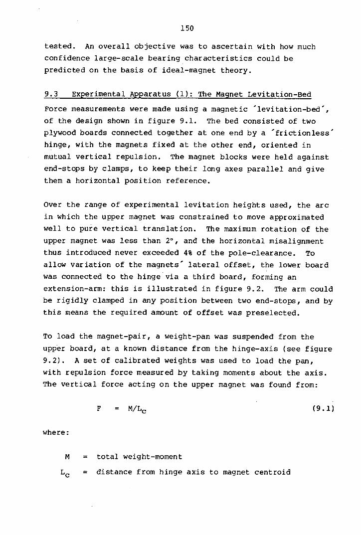
150
tested. An overall objective was to ascertain with how much
confidence large-scale bearing characteristics could be
predicted on the basis of ideal-magnet theory.
9.3 Experimental Apparatus (1): The Magnet Levitation-Bed
Force measurements were made using a magnetic levitation-bed,
of the design shown in figure 9.1. The bed consisted of two
plywood boards connected together at one end by a frictionless
hinge, with the magnets fixed at the other end, oriented in
mutual vertical repulsion. The magnet blocks were held against
end-stops by clamps, to keep their long axes parallel and give
them a horizontal position reference.
Over the range of experimental levitation heights used, the arc
in which the upper magnet was constrained to move approximated
well to pure vertical translation. The maximum rotation of the
upper magnet was less than 2 0 , and the horizontal misalignment thus introduced never exceeded 4% of the pole-clearance. To
allow variation of the magnets lateral offset, the lower board
was connected to the hinge via a third board, forming an
extension-arm: this is illustrated in figure 9.2. The arm could
be rigidly clamped in any position between two end-stops, and by
this means the required amount of offset was preselected.
To load the magnet-pair, a weight-pan was suspended from the
upper board, at a known distance from the hinge-axis (see figure
9.2). A set of calibrated weights was used to load the pan,
with repulsion force measured by taking moments about the axis.
The vertical force acting on the upper magnet was found from:
F = M/Lc (9.1)
where:
M = total weight-moment
Lc = distance from hinge axis to magnet centroid
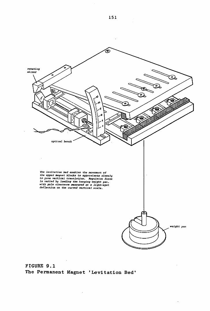
151
rotating mirror
S
optical bench
The levitation bed enables the movement of the upper magnet blocks to approximate Closely to pure vertical translation. Repulsion force Is varied by loading the hanging weight pan, with pole clearance measured as a light-spot deflection on the curved vertical scale.
weight pan
FIGURE 9.1 The Permanent Magnet 'Levitation Bed'
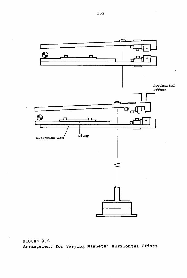
horizontal offset
I r I I
extension arm
FIGURE 9.2 Arrangement for Varying Magnets' Horizontal Offset
152
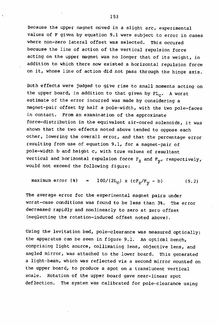
153
Because the upper magnet moved in a slight arc, experimental
values of F given by equation 9.1 were subject to error in cases
where non-zero lateral offset was selected. This occured
because the line of action of the vertical repulsion force
acting on the upper magnet was no longer that of its weight, in
addition to which there now existed a horizontal repulsion force
on it, whose line of action did not pass through the hinge axis.
Both effects were judged to give rise to small moments acting on
the upper board, in addition to that given by FLc . A worst estimate of the error incurred was made by considering a
magnet-pair offset by half a pole-width, with the two pole-faces
in contact. From an examination of the approximate
force-distribution in the equivalent air-cored solenoids, it was
shown that the two effects noted above tended to oppose each
other, lowering the overall error, and that the percentage error
resulting from use of equation 9.1, for a magnet-pair of
pole-width b and height c, with true values of resultant
vertical and horizontal repulsion force F2 and Fy, respectively, would not exceed the following figure:
maximum error (%) = 100/( 2Lc ) x (cF2/F - b) (9.2)
The average error for the experimental magnet pairs under
worst-case conditions was found to be less than 3%. The error
decreased rapidly and nonlinearly to zero at zero offset
(neglecting the rotation-induced offset noted above).
Using the levitation bed, pole-clearance was measured optically:
the apparatus can be seen in figure 9.1. An optical bench,
comprising light source, collimating lens, objective lens, and
angled mirror, was attached to the lower board. This generated
a light-beam, which was reflected via a second mirror mounted on
the upper board, to produce a spot on a translucent vertical
scale. Rotation of the upper board gave near-linear spot
deflection. The system was calibrated for pole-clearance using

154
a vernier height gauge, and the calibration curve stored in
computer memory as an array, to allow both interpolated use, and
correction for magnet pole-width. Zeroing was achieved by
forcing the magnets into pole-contact, and adjusting the
mounting angle of the upper mirror to bring the pointer to scale
zero; maximum systematic error was estimated as 0.5 mm. The
optical method was sensitive, as the spot deflected through
twice the angle of the board's rotation, giving a scale
magnification factor of two.
In addition to that noted above, the sources of uncertainty in
force/clearance measurement were:
scale-reading error
force error due to non-parallellism of magnets
The first of these was small, with half the smallest scale
division corresponding to approximately 0.25 mm. The second
again arose because movement of the magnets was rotational
rather than translational (see figure 9.2): because magnetic
stiffness is nonlinear, a discrepancy was thus introduced in the
measured force. With constant stiffness, no error would have
existed. It was estimated, however, that the fractional error
in force was an order of magnitude lower than the ratio dz/z,
where z is pole clearance, and dz its variation introduced by
the rotation. The worst-case force error (3%) was therefore
adhered to.
The magnets' lateral offset was measured off a horizontal scale
on the lower board, zeroed by lining up the two end-stops on a
square reference-edge. Maximum error was estimated at
approximately 0.3 mm.
To avoid corrupting experimental measurements, most components
of the levitation bed were constructed from non-magnetic
materials. Wood was extensively used, and metal parts were
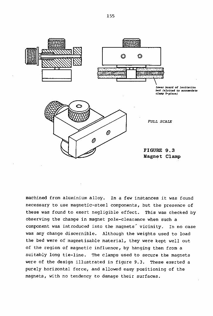
155
lower board of levitation bed (slotted to acconvdate clamp T-piece)
FULL SCALE
FIGURE 9.3 Magnet Clamp
machined from aluminium alloy. In a few instances it was found
necessary to use magnetic-steel components, but the presence of
these was found to exert negligible effect. This was checked by
observing the change in magnet pole-clearance when such a
component was introduced into the magnets' vicinity. In no case
was any change discernible. Although the weights used to load
the bed were of magnetisable material, they were kept well out
of the region of magnetic influence, by hanging them from a
suitably long tie-line. The clamps used to secure the magnets
were of the design illustrated in figure 9.3. These exerted a
purely horizontal force, and allowed easy positioning of the
magnets, with no tendency to damage their surfaces.
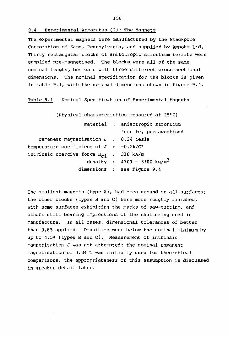
156
9.4 Experimental Apparatus (2): The Magnets
The experimental magnets were manufactured by the Stackpole
Corporation of Kane, Pennsylvania, and supplied by Ainpohm Ltd.
Thirty rectangular blocks of anisotropic strontium ferrite were
supplied pre-magnetised. The blocks were-all of the same
nominal length, but came with three different cross-sectional
dimensions. The nominal specification for the blocks is given
in table 9.1, with the nominal dimensions shown in figure 9.4.
Table 9.1 Nominal Specification of Experimental Magnets
(Physical characteristics measured at 25°C)
material
remanent magnetisation J
temperature coefficient of J
intrinsic coercive force Hci
density
dimensions
anisotropic strontium
ferrite, premagnetised
0.34 tesla
-0.2%/C-
318 kA/m
4700 - 5100 kg/m3
see figure 9.4
The smallest magnets (type A), had been ground on all surfaces;
the other blocks (types B and C) were more roughly finished,
with some surfaces exhibiting the marks of saw-cutting, and
others still bearing impressions of the shuttering used in
manufacture. In all cases, dimensional tolerances of better
than 0.8% applied. Densities were below the nominal minimum by
up to 4.5% (types B and C). Measurement of intrinsic
magnetisation J was not attempted: the nominal remanent
magnetisation of 0.34 T was initially used for theoretical
comparisons; the appropriateness of this assumption is discussed
in greater detail later.
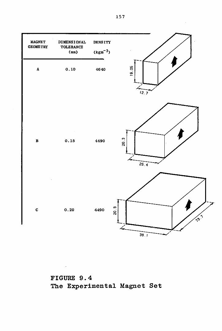
157
MAGNET DIMENSIONAL DENSITY GEOMETRY TOLERANCE
(mm) (kgm 3 )
A 0.10 4640 LI) 0
0)
12.7
B 0.15 4490 C')
Q
C 0.20 4490 C')
0 C'.'
FIGURE 9.4 The Experimental Magnet Set

158
Although only three different block cross-sections were
available, several others were created by clamping together two
or more blocks to form larger magnets. This technique relied on the following assumptions:
A number of magnets damped together with their magnetic
axes oriented in parallel will exhibit the same characteristics
as a single magnet of the same overall size.
A two-dimensional magnet-pair with opposing, ie.
antiparallel, magnetic axes, is exactly equivalent in terms of
force and stiffness as a pair with coparallel, ie.,
side-by-side magnetic axes, as shown in figure 9.5.
The first assumption is verifiable by calculating firstly the
field external to two magnetic blocks placed very close
together, and then that for a single block of the same overall
antiparallel coparallel
With a two-dimensional magnet pair of any geometry, repulsion force and stiffness remain unchanged if the magnetic vectors of the opposing blocks are counter-rotated through the. same angle. Hence the two magnet pairs above will theoretically exhibit the same characteristics. For an explanation of this phenomenon, see Yonnet (1978) or Rowlands (1980).
FIGURE 9.5 Equivalent Configurations for Two-dimensional Magnets
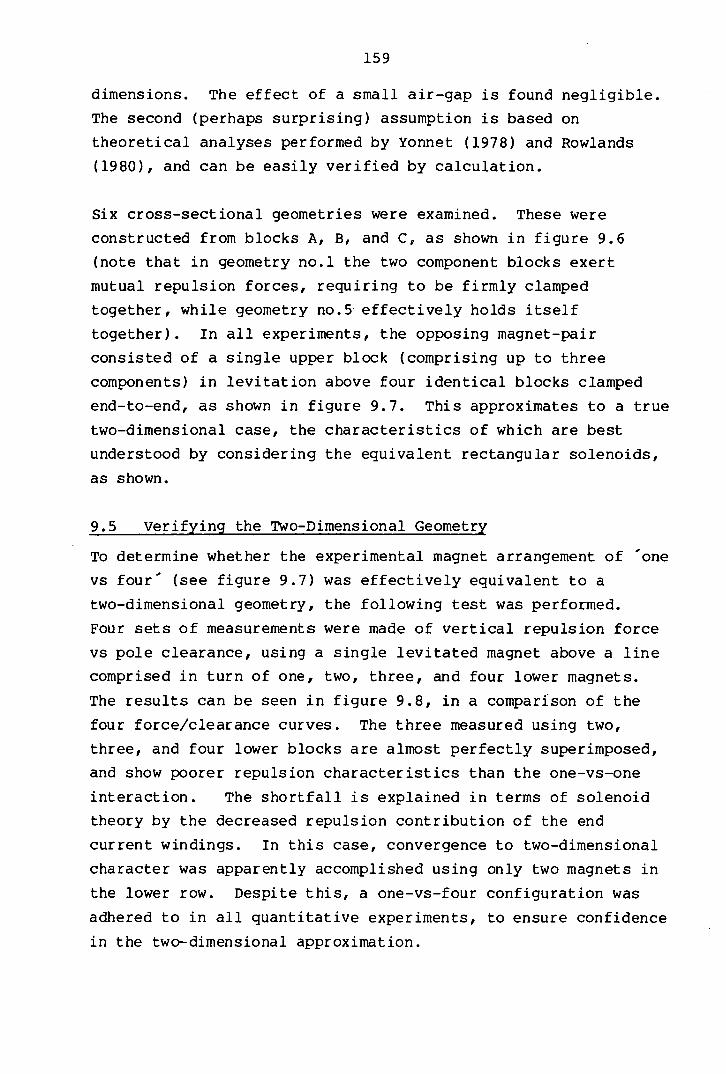
159
dimensions. The effect of a small air-gap is found negligible.
The second (perhaps surprising) assumption is based on
theoretical analyses performed by Yonnet (1978) and Rowlands
(1980), and can be easily verified by calculation.
Six cross-sectional geometries were examined. These were
constructed from blocks A, B, and C, as shown in figure 9.6
(note that in geometry no.1 the two component blocks exert
mutual repulsion forces, requiring to be firmly clamped
together, while geometry no.5 effectively holds itself
together). In all experiments, the opposing magnet-pair
consisted of a single upper block (comprising up to three
components) in levitation above four identical blocks clamped
end-to-end, as shown in figure 9.7. This approximates to a true
two-dimensional case, the characteristics of which are best
understood by considering the equivalent rectangular solenoids,
as shown.
9.5 verifying the Two-Dimensional Geometry
To determine whether the experimental magnet arrangement of 'one
vs four' (see figure 9.7) was effectively equivalent to a
two-dimensional geometry, the following test was performed.
Four sets of measurements were made of vertical repulsion force
vs pole clearance, using a single levitated magnet above a line
comprised in turn of one, two, three, and four lower magnets.
The results can be seen in figure 9.8, in a comparIson of the
four force/clearance curves. The three measured using two,
three, and four lower blocks are almost perfectly superimposed,
and show poorer repulsion characteristics than the one-vs-one
interaction. The shortfall is explained in terms of solenoid
theory by the decreased repulsion contribution of the end
current windings. In this case, convergence to two-dimensional
character was apparently accomplished using only two magnets in
the lower row. Despite this, a one-vs-four configuration was
adhered to in all quantitative experiments, to ensure confidence
in the two-dimensional approximation.

160
MAGNET - sub- c . aspect PAIR No, blocks
(mm) (mm) ratio b/c
1 A+A
19.05 25.4 0.75:
2 B
3 B
4 2A+B
5 B-i-B
6 C
Iti 4-
[4 . 4
141
20.3 25.4 0.80
25.4 20.3 1.25
39.4 25.4 1.55
40.6 25.4 1.60
38.1 20.3 1.875
U (I
I-
>
horizontal
FIGURE 9.6 Experimental Magnet Pair Geometries
Jo

imation may be explained using solenoid theory. Forces exist only between parallel current-carrying wires; in the above configuration the end interactions are thus relatively weak. Note too the cancelling of internal currents.
161
The 'one vs four' experimental configuration is used to approximate a two-dimensional magnet pair interaction. A single upper block is levitated above the mid-point of a line of four similar blocks.
FIGURE 9.7 Explanation of Two-dimensional Magnet Approximation
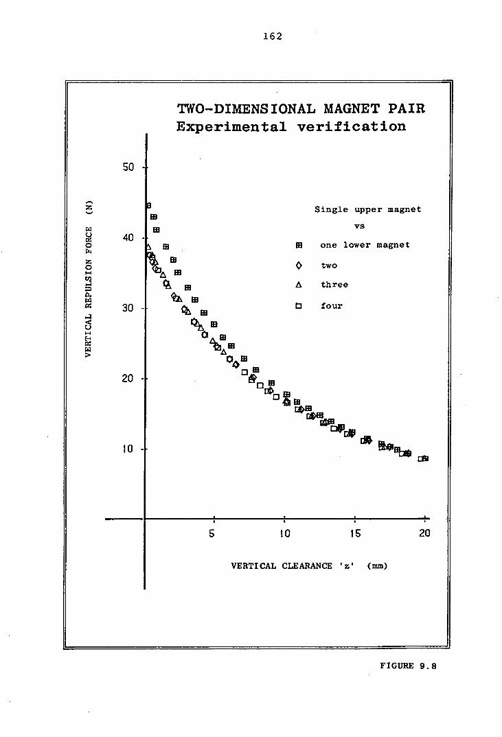
162
TWO-DIMENSIONAL MAGNET PAIR Experimental verification
30
PI-11
Ic
Single upper magnet
vs
M is one lower magnet
G two
CA M A three
0 four
E ffl
E3 M &0 1B
cm
S 10 iS 20
VERTICAL CLEARANCE ' ( mm)
so -
z
0
40 - w 0
z 0
FIGURE 9.8
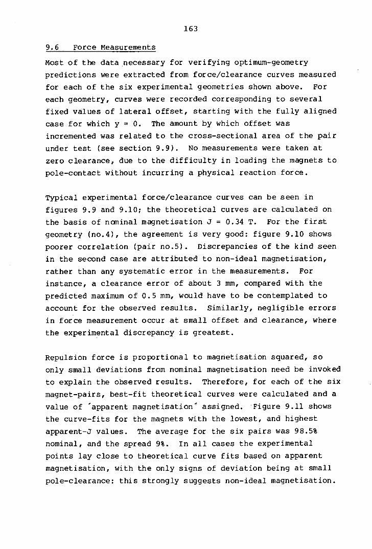
163
9.6 Force Measurements
Most of the data necessary for verifying optimum-geometry
predictions were extracted from force/clearance curves measured
for each of the six experimental geometries shown above. For
each geometry, curves were recorded corresponding to several
fixed values of lateral offset, starting with the fully aligned
case for which y = 0. The amount by which offset was
incremented was related to the cross-sectional area of the pair
under test (see section 9.9). No measurements were taken at
zero clearance, due to the difficulty in loading the magnets to
pole-contact without incurring a physical reaction force.
Typical experimental force/clearance curves can be seen in
figures 9.9 and 9.10; the theoretical curves are calculated on
the basis of naninal magnetisation J = 0.34 T. For the first
geometry (no.4), the agreement is very good: figure 9.10 shows
poorer correlation (pair no.5). Discrepancies of the kind seen
in the second case are attributed to non-ideal magnetisation,
rather than any systematic error in the measurements. For
instance, a clearance error of about 3 mm, compared with the
predicted maximum of 0.5 mm, would have to be contemplated to
account for the observed results. Similarly, negligible errors
in force measurement occur at small offset and clearance, where
the experimental discrepancy is greatest.
Repulsion force is proportional to magnetisation squared, so
only small deviations from nominal magnetisation need be invoked
to explain the observed results. Therefore, for each of the six
magnet-pairs, best-fit theoretical curves were calculated and a
value of 'apparent magnetisation assigned. Figure 9.11 shows
the curve-fits for the magnets with the lowest, and highest
apparent-J values. The average for the six pairs was 98.5%
nominal, and the spread 9%. In all cases the experimental
points lay close to theoretical curve fits based on apparent
magnetisation, with the only signs of deviation being at small
pole-clearance: this strongly suggests non-ideal magnetisation.
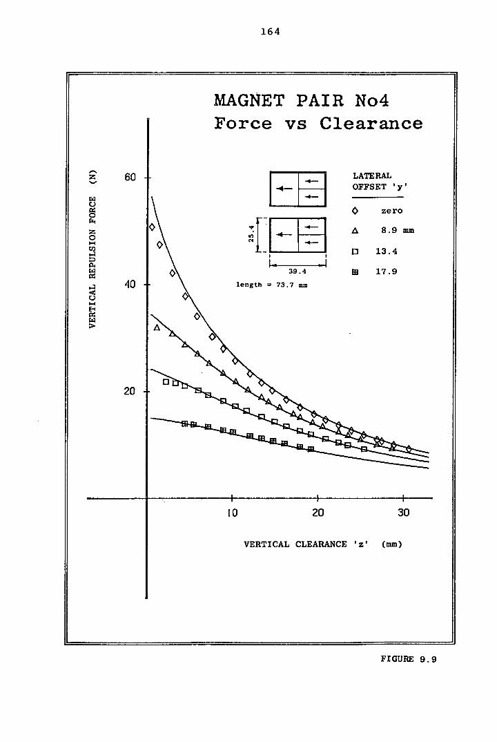
164
MAGNET PAIR No4 Force vs Clearance
60 LATERAL OFFSET 'y'
C) zero
8.9mm IIiH : I \ -, 1] 13.4 ' I
0 39.4 m 17.9 40 length = 73.7 mm
C-)
0
20TB
I I I
10 20 30
VERTICAL CLEARANCE 'z' (mm)
FIGURE 9.9
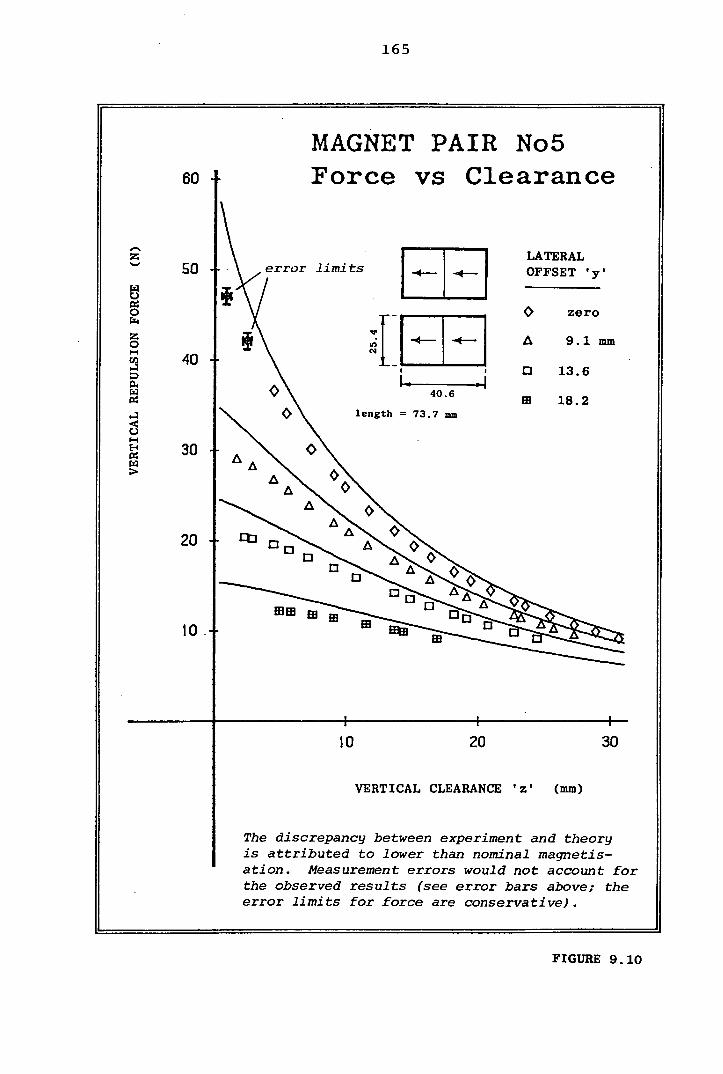
Z
C.)
0 r14
Z
04
0 I-I
C.)
MAGNET PAIR No5 60 Force vs Clearance
LATERAL 50 error limits . ._ OFFSET 'y'
V 0 zero
H-HH 40 \ 13.6
Cq
\ ' \ 40.6
W 18.2 N 0 \ length = 73.7 mm
30
0 20 0 D
13
D
E9 13 0
10.
10 20 30
VERTICAL CLEARANCE ' z ' (mm)
The discrepancy between experiment and theory is attributed to lower than nominal magnetis- ation. Measurement errors would not account for the observed results (see error bars above; the error limits for force are conservative).
FIGURE 9.10
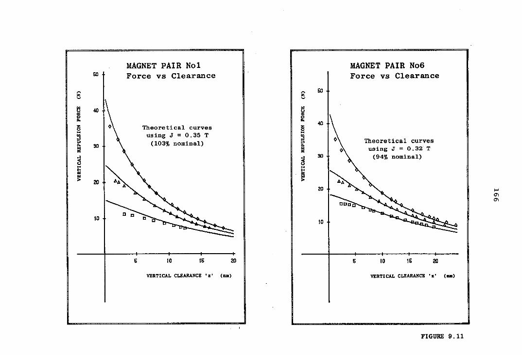
10 13 13
0
6 $0 IS 20
VERTICAL CLEARANCE 'z' (mm)
MAGNET PAIR No6 Force vs Clearance
-.. So z
40\
Theoretical curves using J0.32T
30 (94% nominal)
I LA
:
1300
I I I I
S tO 15 20
VERTICAL CLEARANCE 'z' (mm)
MAGNET PAIR Nol go Force vs Clearance
z
40\
Theoretical curves using J = 0.35 T
0. 30 (103% nominal)
LI 20 Ax
A-.
FIGURE 9.11
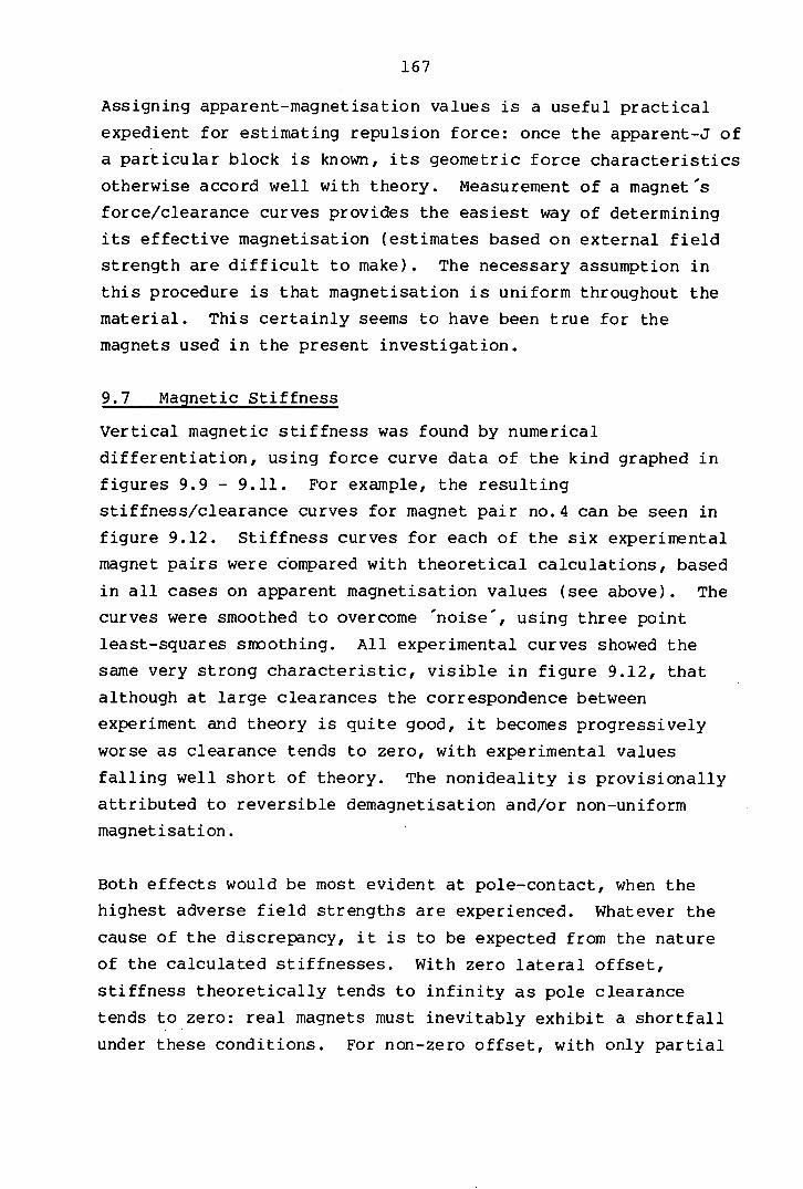
167
Assigning apparent-magnetisation values is a useful practical
expedient for estimating repulsion force: once the apparent-J of
a particular block is known, its geometric force characteristics
otherwise accord well with theory. Measurement of a magnets
force/clearance curves provides the easiest way of determining
its effective magnetisation (estimates based on external field
strength are difficult to make). The necessary assumption in
this procedure is that magnetisation is uniform throughout the
material. This certainly seems to have been true for the
magnets used in the present investigation.
9.7 Magnetic Stiffness
Vertical magnetic stiffness was found by numerical
differentiation, using force curve data of the kind graphed in
figures 9.9 - 9.11. For example, the resulting
stiffness/clearance curves for magnet pair no.4 can be seen in
figure 9.12. Stiffness curves for each of the six experimental
magnet pairs were compared with theoretical calculations, based
in all cases on apparent magnetisation values (see above). The
curves were smoothed to overcome noise, using three point
least-squares smoothing. All experimental curves showed the
same very strong characteristic, visible in figure 9.12, that
although at large clearances the correspondence between
experiment and theory is quite good, it becomes progressively
worse as clearance tends to zero, with experimental values
falling well short of theory. The nonideality is provisionally
attributed to reversible demagnetisation and/or non-uniform
magnetisation.
Both effects would be most evident at pole-contact, when the
highest adverse field strengths are experienced. Whatever the
cause of the discrepancy, it is to be expected from the nature
of the calculated stiffnesses. With zero lateral offset,
stiffness theoretically tends to infinity as pole clearance
tends to zero: real magnets must inevitably exhibit a shortfall
under these conditions. For non-zero offset, with only partial
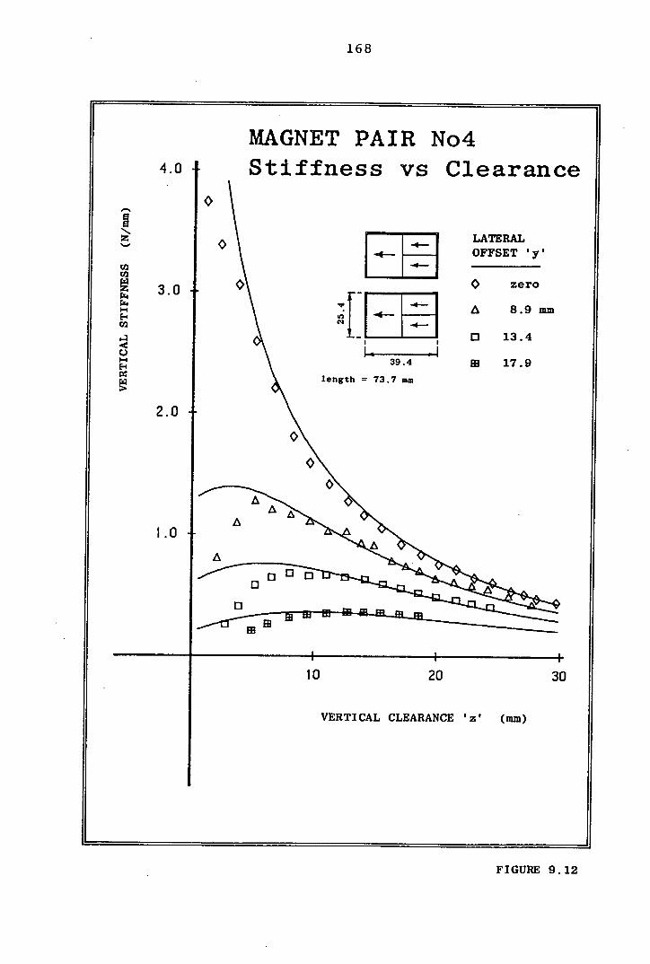
168
MAGNET PAIR No4 4.0 1 Stiffness vs Clearance
0
I
z
________
I I LATERAL ()
4- OFFSET
U) U)
zero r4 I I P4
A 8.9 mm - I,fI.4_I I U) ¶1 Cl 13.4
I I
- 39.4 ifi 17.9 length = 73.7 mm
2.0
0
LU
O DD
10 20 30
VERTICAL CLEARANCE 'z' (mm)
FIGURE 9.12
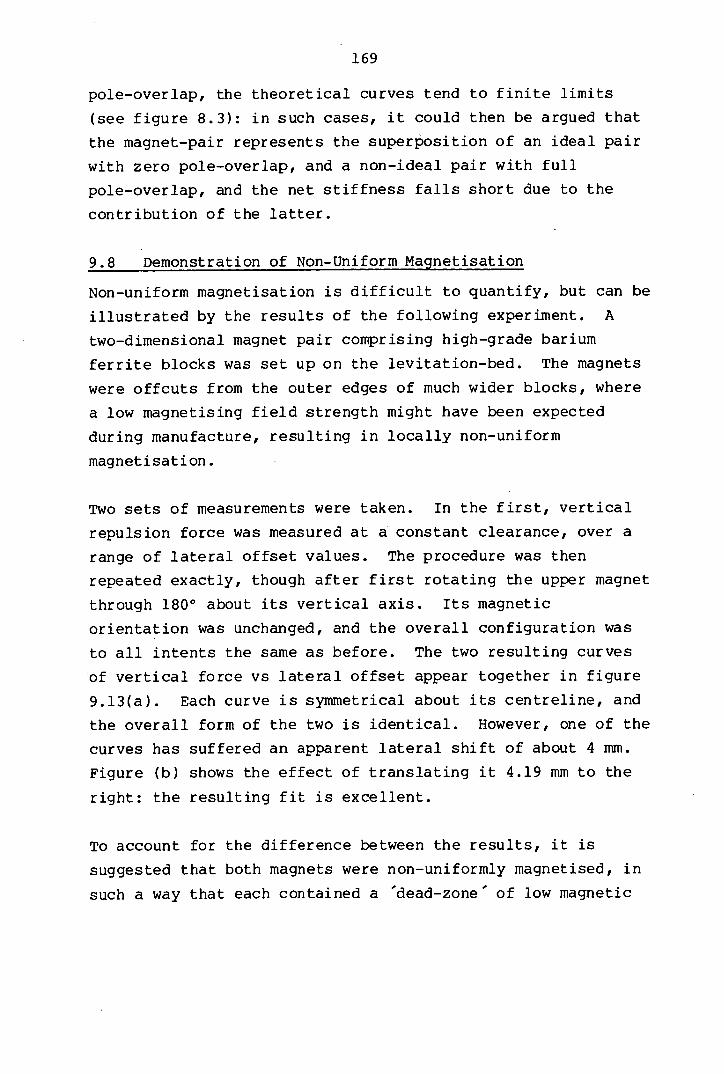
169
pole-overlap, the theoretical curves tend to finite limits
(see figure 8.3): in such cases, it could then be argued that
the magnet-pair represents the superposition of an ideal pair
with zero pole-overlap, and a non-ideal pair with full
pole-overlap, and the net stiffness falls short due to the
contribution of the latter.
9.8 Demonstration of Non-Uniform Magnetisation
Non-uniform magnetisation is difficult to quantify, but can be
illustrated by the results of the following experiment. A
two-dimensional magnet pair comprising high-grade barium
ferrite blocks was set up on the levitation-bed. The magnets
were offcuts from the outer edges of much wider blocks, where
a low magnetising field strength might have been expected
during manufacture, resulting in locally non-uniform
magnetisation.
Two sets of measurements were taken. In the first, vertical
repulsion force was measured at a constant clearance, over a
range of lateral offset values. The procedure was then
repeated exactly, though after first rotating the upper magnet
through 1800 about its vertical axis. Its magnetic
orientation was unchanged, and the overall configuration was
to all intents the same as before. The two resulting curves
of vertical force vs lateral offset appear together in figure
9.13(a). Each curve is symmetrical about its centreline, and
the overall form of the two is identical. However, one of the
curves has suffered an apparent lateral shift of about 4 mm.
Figure (b) shows the effect of translating it 4.19 mm to the
right: the resulting fit is excellent.
To account for the difference between the results, it is
suggested that both magnets were non-uniformly magnetised, in
such a way that each contained a dead-zone of low magnetic
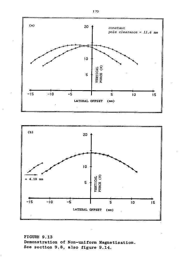
170
(a) c-.J Constant
pole clearance = 11.6 mm
10
is.
LATERAL OFFSET (mm)
FIGURE 9.13 Demonstration of Non—uniform Magnetisation. See section 9.8, also figure 9.14.
171
II II IIsin
apparent _J I offset
In both configurations, the magnet pair is in nominally perfect lateral alignment. However, the existence of non-magnetised 'dead zones' in the two blocks causes the right hand arrangement to behave as though a finite lateral offset existed. Maximum vertical repulsion is then only observed once a real offset, equivalent to the width of the dead zones, has been set (see figure 9.13).
FIGURE 9.14 Non—uniform Magnetisation
strength, as shown in figure 9.14. In the first experiment, the
two dead-zones lined up, and the position of maximum vertical
repulsion corresponded to that of zero nominal offset. In the
second case, rotation of the upper block introduced a built-in
offset, and maximum repulsion was then only observed after the
equivalent real offset.
The results of previous experiments using rare-earth cobalt
magnets (Tsui et al, 1972, Craik and Harrison, 1974, and Yonnet,
1980) have shown better agreement with theory than those of the
present work: the small size of the magnets used in these cases
may well have allowed for a more uniform magnetising field
during manufacture. However, in the design of a large-scale
magnetic bearing such as that in the present case, allowance
172
must be made for the possibility of non-ideal magnetisation.
The results of this study suggest that although ideal magnet
assumptions allow repulsion forces to be predicted with some
degree of confidence, they serve badly when calculating
stiffness at small clearances. A future analysis is recommended
in which allowances for non-uniform and reversible magnetisation
would be included at the the theoretical stage, possibly by
superposing ideal and non-ideal magnets, where the non-ideality
would be clearance-dependent. For practical purposes, however,
an empirical rule for the minimum 'safe' clearance at which
theory holds good is noted at the end of section 9.10.
9.9 Optimum Geometries (1): Constrained Force/Length
The first procedure was an attempt to verify the theoretical
results described in section 8.5. In this, and the subsequent,
examination of constrained geometries, the optimum magnet aspect
ratio b/c was sought for a fixed total area A (= 2bc), over a
range of values of pole-clearance and offset.
Measured values of force/unit length F z were normalised in this
case by dividing by A½. This choice of representative linear
dimension is important: normalising is equivalent to scaling the
representative dimension to unity (see section 8.4), and
the results were thus scaled to represent those for magnet-pairs
all of the same cross-sectional area, allowing direct comparison
of the dependence on aspect ratio. In setting up each
measurement, care was taken to observe geometric similarity of
both pole clearance and offset: for example, in figures 9.9 -
9.11 it can be seen that offset y was incremented in amounts
corresponding to 0.1 x A½. Normalisation also included dividing
by the magnetisation product J 2 , where apparent magnetisation
values (see above) were used throughout. The normalised results
for this first comparison are presented in figures 9.15 and
9.16, as four curve 'families'.
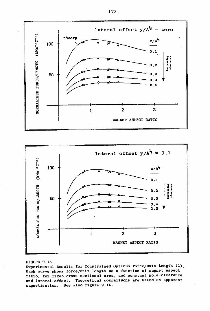
173
lateral offset y/A½ = zero
N theory z/A½
100 r o G
0.1 NV VU
I V I •
0.2 Z I •° Da t . 50 0.3 I
0.4+ 0 0.5 1z4
rzl Ca Pq
o 1 2 3 Z
MAGNET ASPECT RATIO
lateral offset y/A½ = 0.1
N
100 z/A ½ a Z
0.1 NV VU
C, Z
0.2 I! kV
50 0.3
0.4 0.5
(I)
0 1 2 3 Z
MAGNET ASPECT RATIO
FIGURE 9.15 Experimental Results for Constrained Optimum Force/Unit Length (1). Each curve shows force/unit length as a funàtion of magnet aspect ratio, for fixed cross sectional area, and constant pole-clearance and lateral offset. Theoretical comparisons are based on apparent-magnetisation. See also figure 9.16.

174
lateral offset y/A½ = 0.2 N
r 100 a z theory
z/A
0.1
50 0.2 0.3 o .4
do
0 0.4 .4
0.5
'-4
I •__ o z
.1
1 2 3
MAGNET ASPECT RATIO
lateral offset y/A½ = 0.3 N
100 z
z/A½ 0 - z
N. 50 0.1 I do
'-4
0 0 4 0.4
0.3 do .4
C12
I I I o 1 2 3
MAGNET ASPECT RATIO
FIGURE 9.16 Experimental Results for Constrained Optimum Force/Unit Length (2). See caption under figure 9.15.
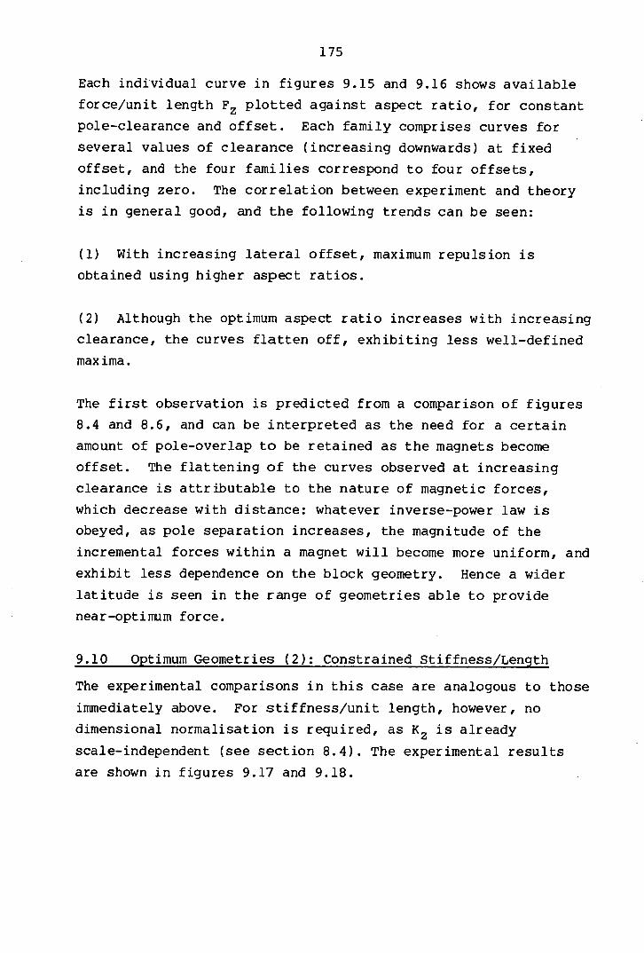
175
Each individual curve in figures 9.15 and 9.16 shows available
force/unit length Fz plotted against aspect ratio, for constant
pole-clearance and offset. Each family comprises curves for
several values of clearance (increasing downwards) at fixed
offset, and the four families correspond to four offsets,
including zero. The correlation between experiment and theory
is in general good, and the following trends can be seen:
With increasing lateral offset, maximum repulsion is
obtained using higher aspect ratios.
Although the optimum aspect ratio increases with increasing
clearance, the curves flatten off, exhibiting less well-defined
maxima.
The first observation is predicted from a comparison of figures
8.4 and 8.6, and can be interpreted as the need for a certain
amount of pole-overlap to be retained as the magnets become
offset. The flattening of the curves observed at increasing
clearance is attributable to the nature of magnetic forces,
which decrease with distance: whatever inverse-power law is
obeyed, as pole separation increases, the magnitude of the
incremental forces within a magnet will become more uniform, and
exhibit less dependence on the block geometry. Hence a wider
latitude is seen in the range of geometries able to provide
near-optimum force.
9.10 Optimum Geometries (2): Constrained Stiffness/Length
The experimental comparisons in this case are analogous to those
immediately above. For stiffness/unit length, however, no
dimensional normalisation is required, as K.is already
scale-independent (see section 8.4). The experimental results
are shown in figures 9.17 and 9.18.
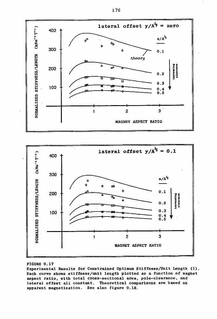
176
r.
t.
H Z
0 Z
Cl) Cl)
rz4
to
FA Cl)
0 Z
lateral offset y/A½ = zero
/ o • 300
theory
200
100
1 2
z/A
0.1
0.2
0.3
0.5
.4
ii
3
MAGNET ASPECT RATIO
lateral offset y/A½ = 0.1 400
t4
300
0 00
200 0.1 to to
0.2 : U -
a
100 0.3 to 0.4
0.5
U)
1 2 3 Z
MAGNET ASPECT RATIO
FIGURE 9.17 Experimental Results for Constrained Optimum Stiffness/Unit Length (1). Each curve shows stiffness/unit length plotted as a function of magnet aspect ratio, with total cross-sectional area, pole-clearance, and lateral offset all constant. Theoretical comparisons are based on apparent magnetisation. See also figure 9.18.
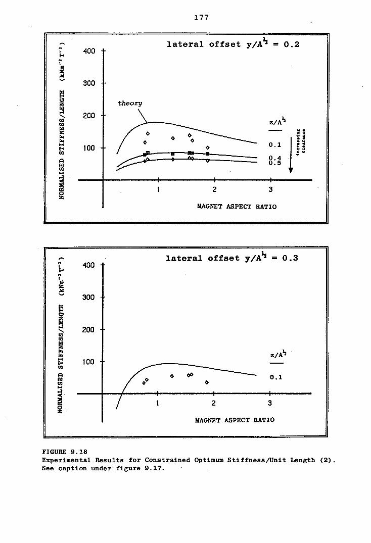
177
lateral offset y/A½ = 0.2 E4 400 C.
z
300
0 z theory
1-1 200 Ca Z/A½ rA
- 0 Cu rZ4 0 *
0.1 I H e: 100 I u I CU
0 0.4
5
r:i
I I 1 2 3
z MAGNET ASPECT RATIO
FIGURE 9.18 Experimental Results for Constrained Optimum Stiffness/Unit Length (2). See caption under figure 9.17.
178
From figures 9.17 and 9.18 it is seen that:
The same trends apply to stiffness/unit length as noted for
force/unit length (see section 9.9).
The shortfall in stiffness at small clearances is strongly
in evidence.
In all cases, correlation with theory becomes good at a value of
z/A½ greater than about 0.3: this is therefore suggested as a
criterion for confidence in theoretical stiffness calculations.
9.11 Optimum Geometries (3): Unconstrained Force/Volume
The results in this section correspond to the theoretical
optimisation procedure of section 8.8. To verify unconstrained
optimisation results, force/unit volume Fv requires to be
investigated in terms not onlyof magnet shape, but also of
size: this reflects the presence of two independent variables in
the unconstrained geometry analyses. Clearly, without a vast
selection of experimental magnets, magnet width and height can
not be independently varied in practice. To circumvent this
problem, the experimental procedure invoked a change of
variables, from pole width b and height c, to aspect ratio b/c,
and cross-sectional area 2bc.
Aspect ratio was varied, as before, by choosing from the six
magnet geometries. Cross-sectional area was necessarily
constant for each magnet-pair, and the method of 'effectively'
varying it made use of the scaling laws. By using the clearance
as representative linear dimension, measured values of Fv were
normalised to represent measurements made at constant clearance,
but with magnets of varying cross-sectional area. Normalisation
involved multiplying measured Fv by z (see section 8.4). This
scaling technique is explained graphically in figure. 9.19, and
the experimental results are shown in figures 9.20 - 9.22.

179
500 FORCE
VOLUME
400
(kNm 3 )
300
200
100
ORIGINAL DATA is force/unit volume for a magnet pair of constant size and increasing pole clearance.
5 10 15
CLEARANCE 'z (mm)
In the initial experiment, the force vs clearance curve is recorded for a fully aligned, symmetric, magnet pair. Because the magnets' volume is necessarily constant, the resulting curve can be plotted as above, as force/unit volume vs clearance. The diagram on the right shows the variation in pole clearance during the experiment.
In order to leave the above results independent of scale, and also effect a tran form of variables, the results are now normalised. Each value of force/unit volume is multiplied by the clearance at which it was measured, while the cZearance itself is replaced by the dimensionless ratio of the square root of magnet cross-sectional area to clearance, ie. ,/(area)/z. The resulting normalised curve is shown below.
2.0
FORCE xz VOLUME
1.5
Wm-2)
1.0
0.5
NORJIAIJSED DATA is force/unit volume at a constant clearance, using a magnet pair of increasing size.
5 10
(AREA) /CLEARANE
Normalising the results is equivalent to scaling them to represent those which would have accrued had the normalising linear dimension been unity (see section 8.4). In the present case the representative dimension is the clearance, and hence the original data can be replotted as force/unit volume measured at constant clearance, for a magnet pair of increasing size (above, right).
The normalised curve exhibits a well-defined maximum, which corresponds to the optimum ratio of magnet size to pole clearance to yield maximum force/unit volume using magnets of this particular aspect ratio. To investigate the dependence on aspect ratio, it is then necessary to repeat the experiment with magnets of several different cross-sectional geometries. The results of such experiments are shown in figures 9.20 - 9.22.
FIGURE 9.19 Results Normalisation. How the scaling laws are used to effect a change of variables.

0, 0
OPTIMUM FORCE/VOLUME (1)
Force/unit volume plotted against magnet cross-sectional size (as the ratio A½/z), for each of six different aspect ratios. Clearance constant, and lateral offset zero, hence y/z = 0; superimposed on each curve is the theoretical maximum force/volume, obtained with aspect ratio 1.461 and A½/z = 2.346.
L L L L L
I y/zzerol
54 0,-s MW
•0 C4 14
II
4.)
80
'4 p14) .4.4
d 4A 0 dO - 0 .4
08
08 0 .4 Q4.) s4. 00
I I I 111111
5
I I II
10 50
(AREA) ½/CLEARANCE
I EI
I!J 04
ca
El
20t ':o
maximui theoretically pOSBible 18.12 kN'
FIGURE 9.20

Wk
L
L 0
0
maximum theoretically - possible - 15.82 kNmT 3
0
k 0
.4
\ 04' 0
$44J 00
0.
k
0.
14 .10. 00
5
I 111111 I I I I
10 50
(AREA) ½/CLEARANCE
L L L L 0 0 0 0
I \ I\ I\ I\ o
I iz = 0.51
OPTIMUM FORCE/VOLUME (2)
Force/unit volume plotted against magnet cross-sectional size.(as the ratio A2/z), for each of six different aspect ratios. Clearance and lateral offset constant, with y/z = 0.5; superimposed on each curve is the theoretical maximum force/volume, obtained with aspect ratio 1.461 and A½/z = 2.996.
15
I 10
S
00
FIGURE 9.21
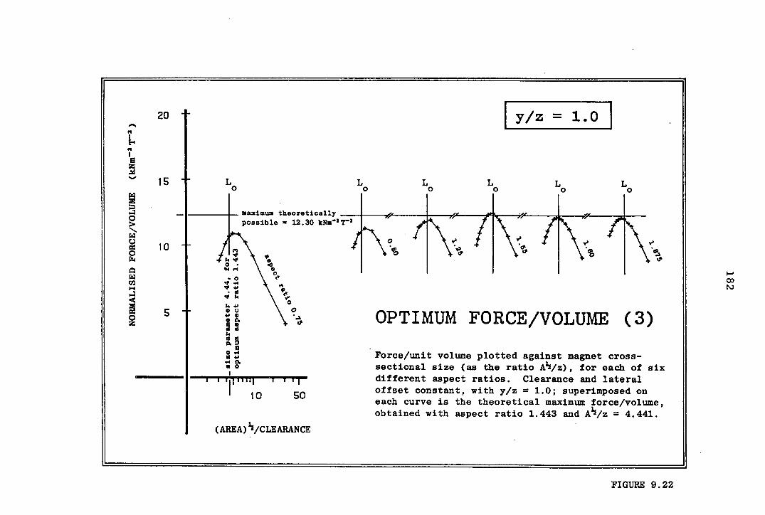
0
IN
20
15 L 0
maximum theoretically possible - 12.30 kNm
I It) # I. 0 \ - 0. •0
0 \c -o
\' eQ 0 \
Is
0.4 0 44
I I 11111111
10 SO
(AREA) s/CLEARANCE
i1
5
I y/z=i.oI
L L L 0 0 0
Wo
OPTIMUM FORCE/VOLUME (3)
Force/unit volume plotted against magnet cross-sectional size (as the ratio A½/z), for each of six different aspect ratios. Clearance and lateral offset constant, with y/z = 1.0; superimposed on each curve is the theoretical maximum force/volume, obtained with aspect ratio 1.443 and A½/z = 4.441.
L (. L
I- 0, 1'.)
FIGURE 9.22
183
Each of figures 9.20 - 9.22 shows six curves, plotted against
the same axis set, which is repeated across the page: this is to
allow comparison of curve maxima. Note that the curves are
formed by joining experimental points, and are not theoretical
fits. All six curves in a given figure correspond to
measurements at a single value of the ratio y/z. Figure 9.20
shows the results for centred magnets, where y/z equals zero.
Each individual curve shows Fv plotted against cross-sectional
size (increasing from left to right) for a given aspect ratio.
The relative efficiencyof different aspect ratios is seen by
comparing curves. The theoretical overall-maximum force/unit
volume Fv for each value of y/z is marked against each curve,
with the axis L0 giving the corresponding optimum size ratio. The results show that:
There is little to choose between aspect ratios in the
range 1.25 to 1.875, which straddle the theoretical optimum in
all three cases.
Prediction of the optimum magnet size is very good indeed,
as demonstrated by the proximity of the curve maxima to the axis
for aspect ratios close to the theoretical optima.
There is practically no shift in the optimum aspect ratio
over a range of y/z values 0 - 1.0.
The uniformly high efficiency noted in (1) above is in keeping
with the theoretically predicted insensitivity of force/unit
volume to aspect ratio (when near the optimum), as discussed in
section 8.8. The negligible shift in optimum aspect ratio b/c
in the range y/z = 0 - 1.0 is as predicted by the flatness of
the appropriate curve in figure 8.13. It may be noted that the
entire contents of figures 920 - 9.22 represent experimental
verification of only three points on the theoretical curve in
figure 8.12.
184
9.12 Optimum Geometries (4): Unconstrained Stiffness/Volume
The results in the final case correspond to the analysis in
section 8.9. The same use was made of the scaling laws as above
(see figure 9.19), except normalisation was this time achieved
by multiplying by clearance squared, according to the rules
noted in section 8.4. Only the case of fully-aligned magnets
(y/z = 0) was considered. The results are shown in figure 9.23,
where the format is that used previously in figures 9.20 - 9.22
(see section 9.11). The important features are:
None of the curves is sufficiently complete to show a
maximum, with all displaying a marked one-sidedness. The
results are less conclusive than those for maximum force/volume.
Notwithstanding (1) above, trends are observable in the
results which suggest that the theoretical optimum aspect ratio
and cross-sectional size are correct.
The one-sided appearance of the experimental curves is due to an
experimental limitation: the leftmost point on each curve
represents the maximum clearance at which a measurement could be
made. Beyond this (leftwards) the supported magnet-weight alone
outstripped available vertical repulsion force. Significantly,
the magnet-pair with aspect ratio 0.75, which yielded the most
complete curve, was the smallest of the six experimental pairs
(see figure 9.6). Because of this, it was able to exert higher
absolute values of force/unit volume than the other pairs, at
equivalent relative values of clearance (ie. in proportion to
cross-sectional size). Expressed differently, if the
experiments were to be repeated with magnets half the size of
those actually used, well-defined maxima would probably be seen
for all six curves. This graphically illustrates the way in
which material efficiency improves as magnet size decreases.
Although the lack of maxima leaves (2) above open to question,
the theoretical curves corresponding to figure 9.23 are shown in
figure 9.24, and these tend to support the suggested trends.
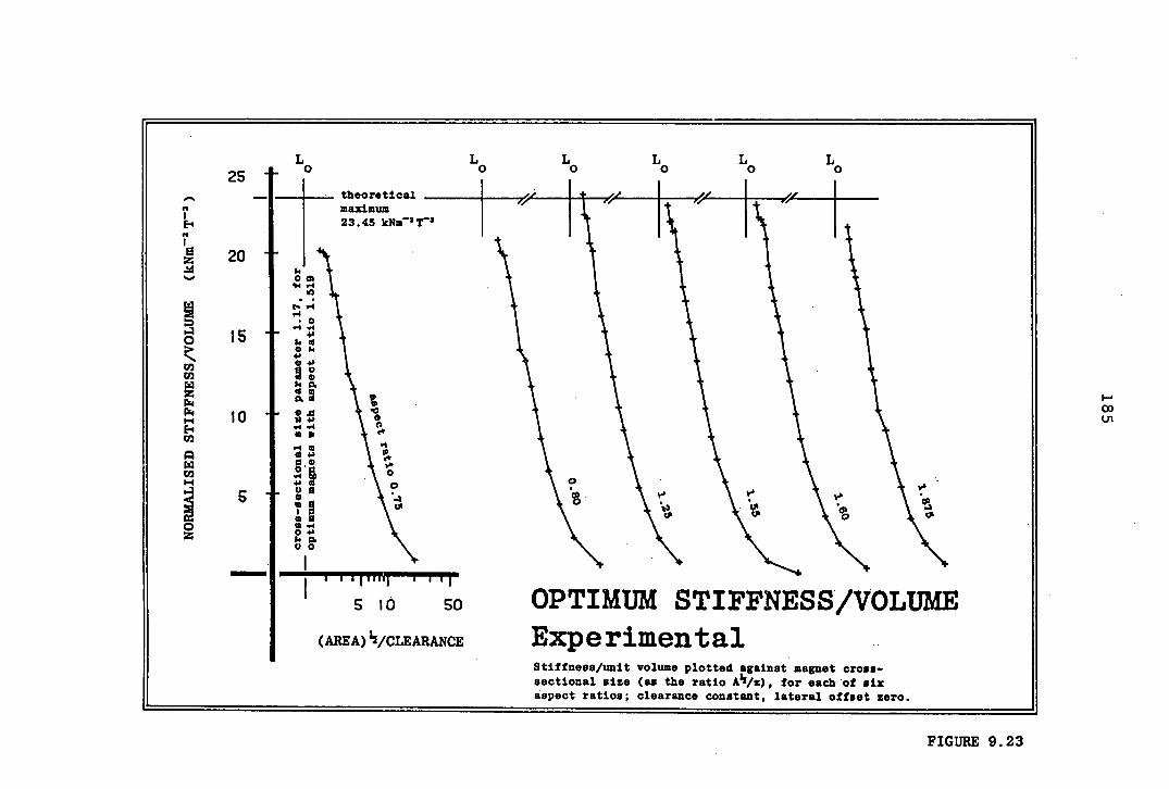
o
..
L
25 °
theoretical maximum 23.45 kNm 3 r
20 I. 00 4 _I
t--1 '4 •0
4'
Ok 4' 04'
Ii.
•0 Ne' 0
'4
'4
0 4J d a
.-1
04' 14 A 00
L L L L L 0 0 0 0 0
0 I-I'
II
ID Z
0
rA rn
I4 P4
rA
to
IR
L;1
S IC SO OPTIMUM STIFFNESS/VOLUME
(AREA)½/CLEARANCE Experimental Stiffness/unit volume plotted against magnet cross-sectional size (as the ratio A'l/z), for each of six aspect ratios; clearance constant, lateral offset zero.
FIGURE 9.23
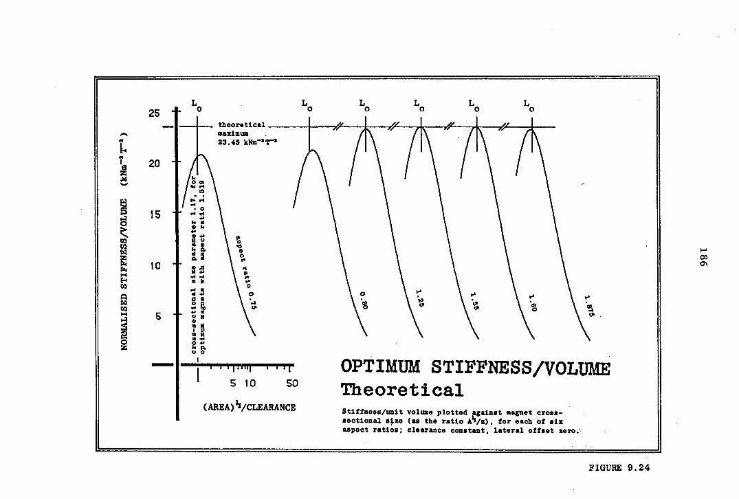
L 25
theoretical maximum 23.45 k a' L " '•
" ik L L L L L
0 0 0 0 0
OPTIMUM STIFFNESS/VOLUME Theoretical Stiffness/unit volume plotted against magnet crosi-sectional size (as the ratio All /s), for each of six aspect ratios; clearance constant, lateral offset zero.
'S
20 $4 7 o
to
15 -I
4' o Oh
4' 04' a) Ho
a) 14
50 a
0. S.
10 .. ,. '4 No'
a) 0 - a 44 a
14 HO o
5 4'S 05 0
an a
'0404' $40. 00
I 11111111 I II
5 10 50
(AREA) h/CLEARANCE
I-' 00 0)
0
' •0' \
FIGURE 9.24

9.13 Conclusions
The experimental evidence presented in this chapter suggests
that the ideal-magnet assumptions of constant and uniform
magnetisation make possible useful calculations of magnetic
force and stiffness, and prediction of optimum geometries,
provided that the following precautions are noted:
Non-ideal magnetisation must be allowed for under certain
circumstances. However, magnets of the type used in this study
can be successfully 'calibrated' and a value of apparent
magnetisation assigned, which replaces the nominal value.
Using apparent magnetisation values, the repulsion force
for a given magnet geometry can be estimated from theory with a
fair degree of accuracy, typically better than 5%, except near
pole contact, where a figure of 10-15% would apply.
The above rule does not apply to theoretical calculations
of stiffness. These are more liable to underpredict the effects
of non-ideal magnetisation, especially near pole contact. An
empirical rule, based on the results of the present study, is
that confidence in theoretical stiffness will be as good as in
force (assuming calibrated magnetisation in both cases) only
when the magnets' pole clearance exceeds about 0.3 times the
square root of their combined cross-sectional area.
Despite the phenomenon of non-ideal magnetisation, the
experimental results tend to reaffirm the theoretical optimum
geometries predicted in chapter 8, for the four analyses dealing
with an isolated two-dimensional magnet pair. However, it
should be noted that real magnet pairs optimised for maximum
stiffness might, if non-ideal magnetisation were taken into
account in the optimisation scheme, require different dimensions
from those predicted in this study.
On a practical note, the technique of transforming experimental
variables, by appropriate use of the scaling laws for magnetic
force, proved highly successful.
CHAPTER 10
SUMMARY AND CONCLUSIONS
10.1 Performance Characteristics of the Proposed Bearing
The design of a novel bearing for use in the Salter duck wave
energy converter has been described, and a preliminary analysis
made of its operating characteristics. The bearing works by
combining the principles of self-pressurising fluid lubrication,
using seawater as the lubricant, and passive permanent magnet
repulsion. Although this combination of features is unusual,
each represents a well-tried bearing mechanism, and the proposed
design brings the two together in an attempt to meet a unique
specification, calling for continuous operation for 25 years in
a marine environment. The intended characteristics of the
bearing include very low friction, evenly distributed loading
with low fluid pressures, compliance, and the ability to
withstand low non-reversing loads indefinitely, and much larger
cyclic loads for periods greatly in excess of their maximum
reversal time.
The lubrication-theory analysis in chapter 4 suggests that the
proposed bearing can comfortably achieve these characteristics,
provided that the appropriate constructional details, which at
this stage are assumed, can be economically realised.
Furthermore, in a reassessment of the bearing's performance
(chapter 5) taking into account effects neglected by lubrication
theory, load enhancement is predicted due to both turbulence and
fluid inertia; even assuming turbulent lubrication, however, the
maximum frictional power loss is estimated as less than 0.1% of
the ducks rated output. One particular aspect of fluid
inertia, the so-called indirect effect, is highly significant,
potentially offering a large increase in load capacity, as well
as an asymmetric bearing response to cyclic loads. Asymmetric
response is necessary to avoid large bearing offsets due to the
non-reversing component of wave loads.
Ime
The indirect effect of fluid inertia takes the form of a static
pressure imbalance occuring across the compliant sheet which
bounds the compressible bearing lining (attached to the inner
surface of the duck). As a result of the imbalance, the
lubricating film thickness is controlled not only by stiffness,
but by the dynamics of the fluid flowing between the lining and
the film. To investigate the magnitude of the effect, a
simplified flow model is proposed, in the form of axisyminetric
radial flow between two parallel discs, either diverging from,
or converging towards, a central orifice. Experimental results,
described in chapter 6, suggest that the minimum dimensionless
pressure drop across such a discharging orifice is a linear
function of reduced Reynolds number, with the constant of
proportionality in fair agreement with previous estimates. The
results also demonstrate the asymmetry of the effect (no
equivalent pressure drop occurs across a recharging orifice),
and the additional head losses which can arise with sharp angled
inlet profiles. This last feature is attributed to flow
separation.
10.2 The Magnetic Repulsion System
Although the use of permanent magnetic repulsion to enhance a
compliant hydrostatic bearing is unorthodox, the combination is,
at least technically, ideal in the present application. Apart
from the necessary axial alignment system, the mechanism can be
entirely non-contacting, and thus not susceptible to wear. It
is the scale of the required bearing which makes the solution
attractive, with the lubricating film thickness dictated by
magnetic repulsion to be proportionally the same as in a
small-scale squeeze film bearing, but with a load capacity
proportionally very much greater. However, it is also the scale
which raises the strongest question regarding the viability of
the bearing. A single duck/spine module might require between
twenty and sixty tonnes of permanent magnets, and it remains to
be proved whether mass production of fairly crude magnets in the
required numbers would be an economic proposition.

190
The magnet optimisation analyses in chapter 8 are all based on
the assumption of ideal hard magnet characteristics, and yield
results applicable to passive permanent magnet bearings on any
scale, not solely that of the duck bearing. A summary of the
more important solutions appears in table 8.1 (p. 147). The
results are intended to allow selection of optimum magnet size
and shape for any given requirement in which an isolated magnet
pair interaction can be assumed. Several of the results are
updates of previous estimates, on which they improve through the
use of computer numerical optimisation techniques. The
experimental observations described in chapter 9 tend to confirm
the theoretical optimum geometries, but also highlight the
deviations from ideality which may occur with real magnets. A
method of calibrating permanent magnets is suggested.
10.3 Bearing Feasibility
The conclusion of this study is that the proposed duck bearing
would be capable of meeting the specification given in chapter
3, provided that certain objectives, which have not yet been
examined, can be met. Of these, perhaps the most important is
to demonstrate that the cost of the permanent magnet repulsion
system, including its axial alignment mechanism, will be
realistic. It has been shown in chapters 7 and 8 that the
better the axial alignment which can be achieved with the
magnets, the smaller they can be. A system in which a lateral
offset of 3 mm could occur might require a total magnet weight
an order of magnitude greater than a (hypothetical) system in
which perfect alignment could be guaranteed (see section 8.13).
It would therefore be wise to invest considerable effort in
perfecting the design of the alignment mechanism.
Other factors must be considered, not least the many
construction details, and the choice of suitable materials
(briefly considered in chapter 3). Although the advantages of
ferrite magnets were propounded in chapter 7, the effects of a

191
25 year immersion in chlorinated seawater on the strengths and
stiffnesses of suitable materials for the compliant bearing
lining remain to be assessed. Methods of attaching the
permanent magnets to the semi-rigid sheet, and to the spine
surface, must also be investigated, and detailed designs
forwarded for the magnet sheet itself, the compressible foam
cells, the axial leakage impedances at the ends of the bearing,
etc. Overall bearing assembly and disassembly, on station if
necessary, has to be carefully planned.
10.4 Suggestions for Further Work
In section 5.9 there was described an analysis, based on the
work of previous authors, which might yield more accurately the
lubrication characteristics of the proposed bearing. The main
advantage of the technique is to allow for a more realistic
model of the orifice discharge flows into the lubricating film,
including the pressure depressions which occur as a result.
However, although this analysis is strongly recommended, it
would be unable to account for the possibilities of turbulent
lubrication, which is very likely to occur, and variation in the
lubricating film thickness, which is essential for exploitation
of the indirect effect of fluid inertia. A mathematical model
which takes account of the latter would be very useful indeed,
as the influence of fluid inertia was seen in chapter 5 to offer
a potentially large decrease in the amount of magnetic material
required.
Another possibility which should perhaps be considered is a
bearing with no magnets at all, in which the low non-reversing
loads were supported by rolling elements of some form, but with
the cyclic loading supported in exactly the same way as in the
current design. The changeover from one load supporting
mechanism to the other could be based on the roller cage
proposal illustrated in figure 3.2 (chapter 3), although it is
to be emphasised that this new design would support the high
reversing loads entirely by fluid lubrication. Some degree of
192
wear would inevitably occur on the rolling elements, but only
under conditions of light loading; the advantages would include
no need for magnets or an axial alignment system, and hence much
lower cost. Alternatively, a study should be carried out to
find a method of producing ferrite magnet blocks in much higher
numbers, but to much lower tolerances (eg. without surface
grinding) than at present. The raw material costs of magnets do
not dominate, and the aim would be to emulate the production of
bricks.
Finally, the need for a representative experimental model is
clear. This would not initially be required to simulate the
conditions of the full bearing specification, but simply to
demonstrate the enhancement of a self-pressurised hydrostatic
bearing by permanent magnet repulsion. Happily, this objective
is now being actively pursued.

193
REFERENCES
Archibald, F. R. (1956): "Load Capacity and Time Relations for
Squeeze Films", Trans. ASME, vol. 78, p. 29-35, Jan. 1956. Baran, W. (1962): "Die Berechnung von Anziehungs- und
Haftkraften für magnetisierte Korper quaderf5rmiger
Gestalt", Zeits. für Angewandte Phys., vol. 14, p. 272,
1962.
Baran, W. (1964): "Zur Bestiminung der Krfte bei Magneten mit
starrer Magnetisierung", Zeits. für Angewandte Phys.,
vol. 17, p. 194-6, 1964.
Baran, W. (1971): "Optieinierung eines permanentmagnetischen
Abstützungssystems für spurgebundene Schnellverkehrsmittel",
Zeits. für Angewandte Phys., vol. 32, p. 216-8, 1971.
Baran, W. (1972): "Der Augenblickliche Stand und die Weitere
Entwicklung auf dem Gebiet der Permanentmagnetischen
Abstützungssyteme für Spurgebundene Schnellverkehrsmittel",
Int. J. Magnetism, vol. 3, p. 103-11, 1972.
Barwell, F. T. (1979): Bearing Systems, Principles and Practice,
Oxford Univ. Press, Oxford, 1979.
Borcherts, R. H. (1971): "Mathematical Analysis of Permanent
Magnet Suspension Systems", J. Appi. Phys., vol. 42, no. 4,
p. 1528-9, 1971.
Box, N. H., Davies, D., and Swann, H. (1969): Nonlinear
Optimisation Techniques, ICI Monograph no. 5, Oliver & Boyd, Edinburgh, 1969.
Castelli, V., Rightmire, G. K., and Fuller, D. D. (1967): "On the Analytical and Experimental Investigation of a
Hydrostatic, Axisymmetric Compliant-Surface Thrust Bearing",
J. Lub. Tech., vol. 89, p. 510-20, 1967.
Castelli, V., Rightmire, G. K., Benjamin, M. K., and Fuller,
D.D. (1969): Design Guide for Hydrostatic Axisyminetric
Compliant Surface Thrust Bearings, Technical Rept. No. 16,
Lubrication Research Lab., Columbia University, New York,
1969.
194
Chen, C. P., and Peube, J. (1964): "Sur lécoulement Radial
Divergent dun Fluide Visqueux Incompressible entre Deux
Plans Paralleles", Comptes Rend. Acad. Sci. (Paris),
vol. t258, no. 22, P. 5353-55, 1964.
Coffey, H. T., Chilton, F., and Hoppie, L. 0. (1972): The
Feasibility of Magnetically Levitating High Speed Ground
Vehicles, US Federal Railroad Admin. Rept. No. FRA-RT-72-39,
Stanford Res. Inst., Menlo Pk., Calif., 1972.
Constantinesdu, V. K. (1962): "Analysis of Bearings Operating in
a Turbulent Regime", J. Basic Eng., vol. 84, p. 139-51,
1962. Cooper, R. K., Neil, V. K., and Woodruff, W. R. (1973): "Optimum
Permanent Magnet Dimensions for Repulsion Applications",
IEEE Trans. Mag., vol. MAG-9, no. 2, p. 125-7, June, 1973.
Craik, D. J. (1966): "Magnetic Fields from Subdivided Surfaces",
British J. Appl. Phys., vol. 17, p. 873-8, 1966.
Craik, D. J. (1967): "Demagnetising Fields in Uniformly
Magnetised Rectangular Prismatic Crystals", British J. Appl.
Phys., vol. 18, p. 1355-6, 1967.
Craik, D. J., and Harrison, A. J. (1974): "Magnetic Field,
Potential, Force and Energy Calculations for Permanent
Magnets", Procs. 3rd European Conference on Hard Magnetic
Materials, p. 33-6, Amsterdam, 1974.
Davies, S. J., and White, C. N. (1928): Proc. Roy. Soc. London,
vol. 119A, p. 92, 1928.
Dowson, D. (1967): "Modes of Lubrication in Human Joints",
Procs. Symposium on Lubrication and Wear in Living and
Artificial Human Joints, London, April, 1967, paper no. 12,
pub. Inst. Mech. Engnrs., London, 1967.
Dowson, D., and Taylor, C. M. (1967): "Elastohydrostatic
Lubrication of Circular Plate Thrust Bearings", J. Lub.
Tech., vol. 89, p. 237-44, July, 1967.
Earnshaw, S. (1839): "On the Nature of the Molecular Forces
which Regulate the Constitution of the Lurniniferous Ether",
Trans. Cambridge Phil. Soc., vol. 7, part 1, p. 97-112,
1839.
195
ETSU (1985a): Wave Energy - The Department of Energy's R & D
Programme 1974-1983, ETSU R26, AERE Harwell, pub. HMSO,
March 1985.
ETSU (1985b): Prospects for the Exploitation of the Renewable
Energy Technologies in the United Kingdom, ETSU R30, AERE
Harwell, pub. HMSO, May 1985.
Henning, G. (1973): "Optiemierung einer gleichgepolten
Magnetanordnung als Abstiitzungssystem für eine
Magnetschwebebahn", Technische Mitteilungen Krupp, vol. 31,
p. 1-10, 1973.
Hudson, J. A., Phillips, D. C., Wilkins, N. J. fi., Davidson, R.,
and Scott, P. M. (1982): Materials Aspects of Wave Energy
Converters, Rept. WESC (82) S P151, AERE Harwell, 1982.
Ishizawa, S. (1965): "The Axisyinmetric Laminar Flow in an
Arbitrarily Shaped Narrow Gap (1st Report, Theoretical
Analysis for the Inlet Region)", Bull. JSME, vol. 8, no. 31,
p. 353-67, 1965.
Ishizawa, S. (1966): "The Axisyininetric Laminar Flow in an
Arbitrarily Shaped Narrow Gap (2nd Report, Theoretical
Analysis of the Downstream Region)", Bull. JSME, vol. 9,
no. 33, p. 86-103, 1966.
Jackson, J. D., and Symmons, G. R. (1965a): "The Pressure
Distribution in a Hydrostatic Thrust Bearing", mt. J. Mech.
Sci., vol. 7, p. 239-42, 1965.
Jackson, J. D., and Syrrunons, G. R. (1965b): "An Investigation of
Radial Laminar Flow Between Two Parallel Discs", Applied
Scientific Research (section A), vol. 15, p. 59-75, 1965.
Jeffrey, D. C., Keller, G. J., Mollison, D., Richmond, D. J. E.,
Salter, S. H., Taylor, J. R. M., and Young, I. (1978):
"Study of Mechanisms for Extracting Power from Sea Waves",
Edinburgh University Wave Power Project 4th Year Report,
July 1978.
Kawashima, G. (1976): "An Experimental Study on Flat Disk
Valves", Bull. JSME, vol. 19, no. 130, p. 420-5, April,
1976.
196
Kawashima, G. (1978): "An Experimental Study on Flat Disk Valves
(2nd Report: the Case of a Rounded Inlet Corner of
Clearance)", Bull. JSME, vol. 21, no. 160, P. 1500-6,
October, 1978.
Kip, A. F. (1969): Fundamentals of Electricity and Magnetism,
2nd edn., McGraw-Hill Kogakusha, Tokyo, 1969.
Kreith, F. (1965): "Reverse Transition in Radial Source Flow
Between Two Parallel Plates", The Physics of Fluids, vol. 8,
no. 6, p. 1189-90, June, 1965.
Kreysig, E. (1983): Advanced Engineering Mathematics, 5th edn.,
Wiley and Sons, New York, 1983.
Kuzma, D. C. (1970): "Determination of the Integration Constant
for Squeeze Films in Infinitely Long Journal Bearings",
J. Lub. Tech., vol. 92, p. 179-80, January, 1970.
Lee, A. J., and Ramster, J. W., editors (1981): Atlas of the
Seas around the British Isles, 1st edn., Ministry of
Agriculture, Fisheries & Food, pub. HMSO, 1981.
Levy, S. B . , and Coogan, C. H., Jr. (1968): "Flexible Membrane
Hydrostatic Air Bearing", J. Lub. Tech., vol. 90, p. 184-90,
January, 1968.
Livesey, J. L. (1959): "Inertia Effects in Viscous Flows", mt.
J. Mech. Sci., vol. 1, p. 84-88, 1959.
Massey, B. S. (1979): Mechanics of Fluids, 4th edn., Van
Nostrand Reinhold (UK) Ltd., Berkshire, 1979.
Maxwell, J. C. (1873): Electricity and Magnetism, 3rd edn.,
vol. 2, Clarendon Press, Oxford, 1873.
McCaig, M. (1961): "Permanent Magnets for Repulsion Systems",
Electrical Review, vol. 15, p. 425-8, September, 1961.
McCaig, N. (1968): "present and Future Technological
Applications of Permanent Magnets", IEEE Trans. Mag.,
vol. MAG-4, no. 3, p. 221-8, September, 1968.
McCaig, N. (1977): Permanent Magnets in Theory and Practice,
Pentech Press, London, 1977.
McCutchen, C. W., and Lewis, P. R. (1959): "Mechanism of Animal
Joints" (two papers), Nature, vol. 184, p. 1284-5, October
24th, 1959.
197
McCutchen, C. W. (1967): "Physiological Lubrication",
Procs. Symposium on Lubrication and Wear in Living and
Artificial Human Joints, London, April, 1967, paper no. 1,
pub. Inst. Mech. Engnrs., London, 1967.
McGinn, J. H. (1955): "Observations on the Radial Flow of Water
Between Fixed Parallel Plates", Applied Scientific Research
(section A), vol. 5, p. 255-64, 1955.
Mime, A. A. (1965): "Inertia Effects in Self Acting Bearing
Lubrication", Procs. mt. Syrnp. on Lubrication and Wear,
Houston, Texas, June, 1963, p.423-527, pub. McCutchen,
Berkeley, Calif., 1965.
Minnich, S. H. (1971): Vehicle Levitation by Rare Earth
Permanent Magnets, General Electric Co. Rept. No. 71-C-104,
Schenechtady, New York, March, 1971.
Moller, P. S. (1963): "Radial Flow Without Swirl Between
Parallel Plates", Aeronautical Quarterly, vol. 14,
p. 163-86, May, 1963.
Mori, H., and Yabe, H. (1966): "Analysis of an Externally
Pressurised Thrust Collar Gas Bearing with Multiple Supply
Holes", Bull. JSME, vol. 9, no. 35, p. 592-9, 1966.
Mori, H., and Yabe, H. (1967): "Design Equations and Charts of
Externally Pressurised Thrust Gas Bearings", Procs. Gas
Bearing Symp., University of Southampton, April, 1967, paper
no. 8.
Ng, C., and Pan, C. H. T. (1965): "A Linearised Turbulent
Lubrication Theory", J. Basic Eng., vol. 87, p. 675-88,
1965.
Orcutt, F. K. (1965): "Investigation of a Partial Arc Pad
Bearing in the Superlaminar Flow Regime", J. Basic Eng.,
vol. 87, p. 145-52, 1965.
Patrat, J. (1975): "Contribution a ltude des Pressions dans un EcouleiTient Radial Divergent", Journal de M&anique, vol. 14,
no. 3, p. 505-22, 1975.
Peube, J. (1963): "Sur 1cou1ement Radial Permanent dun Fluide
Visqueux Incompressible entre Deux Plans Parall1es Fixes",
Journal de Mcanique, vol. 2, no. 4, p. 377-95, 1963.
Picken, M. J., and Fitzgerald, G. M. F. (1981): Report on the
Environmental Factors Relating to the Bristol Cylinder Wave
Energy Device, prep. for Sir Robert McAlpine & Sons Ltd.
under Dept. of Energy contract, Scottish Marine Biological
Assoc., Dunstaffnage, Oban, September, 1981.
Raal, J. D. (1978): "Radial Source Flow Between Parallel Disks",
J. Fluid Mech., vol. 85, part 3, p. 401-16, 1978.
Rabinowicz, E. (1968): Standard Handbook of Lubrication
Engineering, ASME, ed. O'Connor, J. J., and Boyd, J.,
chapter 1, McGraw Hill, New York, 1968.
Rayleigh, Lord (1917): "A Simple Problem in Forced lubrication",
Engineering, December 14th, 1917, p. 617.
Rowlands, G. (1980): "On the Invariance of the Magnetic Field
Strength due to a Uniformly Magnetised Body", IEEE Trans.
Mag., vol. MAG-16, no. 2, p. 480-1, March, 1980.
Salter, S. H. (1974): "Wave Power", Nature, vol. 249, no. 5459,
p. 720-4, June 21st, 1974.
Salter, S. H. (1978): "The Development of the Duck Concept",
Proc. Wave Energy Conf., Heathrow, London, November, 1978,
paper no. 2, p. 17-27, pub. HMSO, 1978.
Salter, S. H. (1980): "Recent Progress on Ducks", Proc. lEE,
vol. 127, part A, no. 5, p. 308-19, June, 1980.
Salter, S. H. (1981a): "Wave Energy - Problems and Solutions",
Journal of the ISA, vol. 129, no. 5301, p. 568-83, August,
1981.
Salter, S. H. (1981b): "Absorbing Wavemakers and Wide Tanks",
Procs. Conf. on Directional Wave Spectra Applications,
Berkeley, Calif., sponsored by Am. Soc. Civil Engnrs.,
September, 1981.
Savage, S. B. (1964): "Laminar Radial Flow Between Parallel
Plates", Trans. ASME, J. Appl. Mech., vol. 31, p. 594-6,
December, 1964.
Schlichting, H. (1979): Boundary Layer Theory, 7th (English)
edn., McGraw-Hill,-New York, 1979, p. 186.
Shaw, R. (1982): Wave Energy - A Design Challenge, Ellis Horwood
Ltd. (distrib. Wiley), Chichester, 1982.
199
Silvester, R. (1974): Coastal Engineering 1 - Generation,
Propagation and Influence of Waves (Developments in
Geotechnical Engineering, vol. 4A), Elsevier Scientific Pub.
Co., Amsterdam, 1974, p. 87.
Smith, N. I., and Fuller, D. D. (1956): "Journal Bearings
Operating at Superlaminar Speeds", Trans. ASME, vol. 78,
p. 469, 1956.
Stansfield, F. N. (1970): Hydrostatic Bearings for Machine Tools
and Other Applications, Machinery Pub. Co. Ltd., Brighton,
Sussex, 1970.
Tsui, J. B. Y., Iden, D. J., Strnat, K. J., and Evers, A. J.
(1972): "The Effect of Intrinsic Magnetic Properties on
Permanent Magnet Repulsion", IEEE Trans. Mag., vol. MAG-8,
no. 2, p. 188-94, June, 1972.
Van Dyke, M. (1970): "Entry Flow in a Channel", J. Fluid Mech.,
vol. 44, part 4, p. 813-23, 1970.
Vohr, J. H. (1969): "A Study of Inherent Restrictor
Characteristics for Hydrostatic Gas Bearings", Proc. 4th
Biannual Gas Bearing Symp., University of Southampton,
April, 1969, vol. 2, paper no. 30.
Ward-Smith, A. J. (1980): Internal Fluid Flow, Clarendon Pres,
Oxford, 1980.
Wilcock, D. F. (1977): "Design of Efficient Turbulent Thrust
Bearings", J. Lub. Tech., vol. 99, p. 113-21, 1977.
Wilson, S. D. R. (1972): "A Note on Laminar Radial Flow Between
Parallel Plates", Applied Scientific Research, vol. 25,
p. 349-54, February, 1972.
Yonnet, J. P. (1978a): "Passive Magnetic Bearings", Proc. Third
International Workshop on Rare Earth Cobalt Magnets and
their Applications, University of California, San Diego,
1978, paper IV-7, p. 241-51.
Yonnet, J. P. (1978b): "Passive Magnetic Bearings with Permanent
Magnets", IEEE Trans. Mag., vol. MAG-14, no.5, p. 803-5,
1978.
200
Yonnet, J. P. (1980): "Etude des Paliers Magnetiques Passifs",
PhD thesis, 1Universit Scientifigue et Mdica1e,
llnstitut National Polytechnigue, Grenoble, July, 1980.
Yonnet, J. P. (1981a): "Permanent Magnet Bearings and
Couplings", IEEE Trans. Mag., vol. MAG-17, no.1, p. 1169-72,
January, 1981.
Yonnet, J. P. (1981b): "Analytical Calculations of Magnetic
Bearings", Fifth International Workshop on Rare Earth Cobalt
Permanent Magnets, Roanoke, Virginia, June, 1981, paper
no. V-3, p. 199-216.
201
ACKNOWLEDGEMENTS
In conclusion, I would like to thank my supervisor, Stephen
Salter, for his help and guidance during my term of study. The
frequently-sought advice of Dr George Alder and Dr David Boffey
has also been much appreciated. For valuable discussion on the
subject of magnetic repulsion, the correspondence of
Dr Jean-Paul Yonnet of Grenoble, and Dr Werner Baran of Essen,
is gratefully acknowledged, and thanks are due to Ken Boyle,
Sarah Hemming, and Mrs Sylvia Furness for translation of the
German maglev' publications. Jamie Taylor took the photograph
which appears in plate 6.2, and Sandy Nelson ran the tank tests
which yielded the wave traces shown in figure 4.3.
The work was financially supported by the Science and
Engineering Research Council, John Laing plc, the Norwegian
Institute of Technology at the University of Trondheim, and the
Edinburgh University Department of Mechanical Engineering. The
UK Department of Energy are to be thanked for the use of their
microcomputing facilities, and for tolerating my occasional
forays into the wavepower mechanical workshop.
Finally, my sincere thanks go to all the past and present
members of the Edinburgh Wave Power Project who placed at my
disposal their advice, encouragement, but most of all
friendship, over the last four years.
CGA
November 22nd 1985