Federal Reserve Bank of New YorkStaff Reports

Fiscal Multipliers and Policy Coordination

Gauti B. Eggertsson

Staff Report no. 241March 2006

This paper presents preliminary findings and is being distributed to economistsand other interested readers solely to stimulate discussion and elicit comments.The views expressed in the paper are those of the author and are not necessarilyreflective of views at the Federal Reserve Bank of New York or the FederalReserve System. Any errors or omissions are the responsibility of the author.

Fiscal Multipliers and Policy CoordinationGauti B. EggertssonFederal Reserve Bank of New York Staff Reports, no. 241March 2006JEL classification: E52, E63

Abstract

This paper addresses the effectiveness of fiscal policy at zero nominal interest rates. I analyze a stochastic general equilibrium model with sticky prices and rationalexpectations and assume that the government cannot commit to future policy. Realgovernment spending increases demand by increasing public consumption. Deficitspending increases demand by generating inflation expectations. I derive fiscal spendingmultipliers that calculate how much output increases for each dollar of governmentspending (real or deficit). Under monetary and fiscal policy coordination, the realspending multiplier is 3.4 and the deficit spending multiplier is 3.8. However, whenthere is no policy coordination, that is, when the central bank is “goal independent,” thereal spending multiplier is unchanged but the deficit spending multiplier is zero.Coordination failure may explain why fiscal policy in Japan has been relatively lesseffective in recent years than during the Great Depression.

Key words: policy coordination, fiscal multiplier, zero interest rates, deflation

Eggertsson: Federal Reserve Bank of New York (gauti.eggertsson@ny.frb.org). This paper is asubstantially revised version of the third chapter of the author’s Ph.D. dissertation, which hedefended at Princeton University in 2004. The author thanks Ben Bernanke, Maurice Obstfeld,Robert Shimer, Chris Sims, Lars E.O. Svensson, Andrea Tambalotti, and especially his principaladvisor, Michael Woodford, for useful comments and suggestions. The author also thanksBenjamin Pugsley for excellent research assistance. The views expressed in this paper are thoseof the author and do not necessarily reflect the position of the Federal Reserve Bank of NewYork or the Federal Reserve System.

1 Introduction

”It is important to recognize that the role of an independent central bank is differ-

ent in inflationary and deflationary environments. In the face of inflation, which is

often associated with excessive monetization of government debt, the virtue of an in-

dependent central bank is its ability to say ”no” to the government. With protracted

deflation, however, excessive monetary creation is unlikely to be the problem, and a

more cooperative stance on the part of the central bank may be called for.”

- Ben Bernanke, Chairman of the Board of Governors of the Federal Reserve, before the Japan Society

of Monetary Economics, Tokyo, Japan, May 31, 2003.

"Coordinate, Coordinate

If monetary policy lacks sufficient power on its own to end deflation, the solution is

not to give up but to try a coordinated monetary and fiscal stimulus."

— The Economist, June 2003, editorial on Japan’s fiscal and monetary policy

The conventional wisdom about monetary and fiscal policy is as follows1: “The first line of

defence against an economic slump is monetary policy: the ability of the central bank — the

Federal Reserve, the European central bank, the Bank of Japan — to cut interest rates. Lower

real interest rates persuade businesses and consumers to borrow and spend, which creates new

jobs, encourages people to spend more, and so on. Since the 1930’s this strategy has worked.

Specifically, interest rate cuts have pulled the US out of each of its big recessions in the past 30

years — in 1975, 1982 and 1991. The second line of defense is fiscal policy: If cutting interest rates

is not enough to support the economy, the government can pump up demand by cutting taxes or

its own spending. The conventional wisdom among economic analysts is that fiscal policy is not

necessary to deal with most recessions, that interest rate policy is enough. But the possibility of

fiscal action always stands in reserve.”

When the central bank has cut the short-term nominal interest rate to zero, the second line

of defense may be needed, especially if the economy faces excessive deflation. Many economists

believe it was wartime government spending that finally pulled the US out of the Great Depression,

a period in which the short-term nominal interest rate had been close to zero for several years.

Recent events in Japan, however, raise questions about the effectiveness of fiscal policy. The Bank

of Japan (BOJ) cut the short-term nominal interest rate to zero in 1998 and since then the budget

deficit has ballooned with the gross public debt exceeding 150 percent of GDP today. Yet deflation

persisted and unemployment remained high despite several "fiscal stimulus" programs (although

1The paragraph in the quotation mark is a summary of Krugman’s (2001) account of the conventional wisdom.

1

recent data indicates that the Japenese economy is finally improving, see e.g. Eggertsson and

Ostry (2005) for discussion of the recovery and the role of policy in supporting it). Is standard

fiscal and monetary policy insufficient to curb deflation and increase demand at low interest rates?

Should we overturn the conventional Keynesian wisdom, based on the Japanese experience, as

some economist have argued?2

This paper addresses these questions from a theoretical perspective by analyzing a stochastic

general equilibrium model with sticky prices. The interest rate decline is due to temporary

demand shocks that make the natural rate of interest — i.e. the real interest rate consistent with

zero output gap — temporarily negative, resulting in excessive deflation and an output collapse. I

assume that the government, the treasury, and the central bank, cannot commit to future policy

apart through the issuance of bonds (following Lucas and Stokey (1983) I assume that the treasury

can commit to pay back the nominal value of its debt). The equilibrium concept used throughout

the paper is that of Markov Perfect Equilibria (MPE), a relatively standard solution concept in

game theory, formally defined by Maskin and Tirole (2001).

I analyze two fiscal policy options to increase demand at low interest rates. The first is

increasing real government spending, i.e. raising government consumption (holding the budget

balanced). The second is increasing deficit spending, i.e. cutting taxes and accumulating debt

(holding real government spending constant). The central conclusion of the paper is that either

deficit spending or real government spending can be used to eliminate deflation and increase

demand when the short-term nominal interest rate is zero. Of the two options I find deficit

spending is more effective, both in terms of reducing deflation/increasing output in equilibrium,

and improving aggregate welfare. This conclusion may seem to vindicate the conventional wisdom.

There are, however, at least three twists to the conventional Keynesian wisdom. First, deficit

spending is only effective if fiscal and monetary policy are coordinated. If there is no coordination,

deficit spending has no effect. This may help explain the weak response of the Japanese economy

to the deficits in recent years. I argue that this is because the deficit spending has not been

accumulated in the context of a coordinated reflation program by the Ministry of Finance and

the Bank of Japan, in contrast to the coordinated reflation policy in the US and Japan during

the Great Depression. Second, real government spending does not only work through current

spending as the conventional wisdom maintains. It also works through expectations about future

spending. Indeed, under optimal fiscal policy, expectations about future spending are even more

important than current spending, contrary to the old fashion IS-LM model where expectations

are fixed. Third, as described in better detail below, the quantitative effectiveness of fiscal policy

is much larger than found by the traditional literature, especially when monetary and fiscal policy

are coordinated.2See e.g. Krugman (2001).

2

Coordinated SolutionThe central bank and the treasury jointly maximize social welfare.

Uncoordinated Solution(“Goal independent” central bank)

Central BankSets it or mt

TreasurySets Ft and Tt

The central bank minimizes:

∑∞

=

+0

220 ][

ttxt

t xE λπβThe treasury maximizes

social welfare

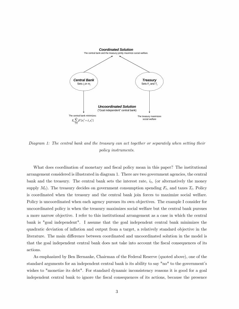
Diagram 1: The central bank and the treasury can act together or separately when setting their

policy instruments.

What does coordination of monetary and fiscal policy mean in this paper? The institutional

arrangement considered is illustrated in diagram 1. There are two government agencies, the central

bank and the treasury. The central bank sets the interest rate, it, (or alternatively the money

supply Mt). The treasury decides on government consumption spending Ft, and taxes Tt. Policy

is coordinated when the treasury and the central bank join forces to maximize social welfare.

Policy is uncoordinated when each agency pursues its own objectives. The example I consider for

uncoordinated policy is when the treasury maximizes social welfare but the central bank pursues

a more narrow objective. I refer to this institutional arrangement as a case in which the central

bank is "goal independent". I assume that the goal independent central bank minimizes the

quadratic deviation of inflation and output from a target, a relatively standard objective in the

literature. The main difference between coordinated and uncoordinated solution in the model is

that the goal independent central bank does not take into account the fiscal consequences of its

actions.

As emphasized by Ben Bernanke, Chairman of the Federal Reserve (quoted above), one of the

standard arguments for an independent central bank is its ability to say "no" to the government’s

wishes to "monetize its debt". For standard dynamic inconsistency reasons it is good for a goal

independent central bank to ignore the fiscal consequences of its actions, because the presence

3

of nominal government debt gives it an inefficient bias to inflate (see e.g. Calvo (1977)). This

remains true in this paper so that in normal circumstances (i.e. in the absence of deflationary

shocks) it is optimal to endow a goal independent central bank with a more narrow mandate

than social welfare. In a deflationary environment, however, this is no longer true so that at least

"temporarily" coordination of monetary and fiscal policy is beneficial, which requires a common

objective of maximizing social welfare, as suggested by Bernanke (2003). Indeed, conditional on

deflationary shocks, coordination is crucial to ensure the effectiveness of fiscal policy as shown in

Table 1 and 2 which summarize the central quantitative results of the paper.

Table 1. Fiscal Multipliers

for Coordinated Policy

Table 2. Fiscal Multipliers

for Uncoordinated Policy

i = 0 i > 0

Real Spending Multiplier 3.37 0.50

Deficit Spending Multiplier 3.76 0.81

i = 0 i > 0

Real Spending Multiplier 3.37 0.50

Deficit Spending Multiplier 0 0

Table 1 and 2 summarize the power of fiscal spending by computing dynamic multipliers. The

first column of Table 1 shows the multipliers under coordination conditional on shocks that make

the zero bound binding. The thought experiment is to compare equilibrium output and fiscal

spending under two scenarios: one when fiscal policy is used for stabilization (either real or deficit

spending), and a second when fiscal policy is inactive. By comparing these two equilibria I can

compute a dynamic multipliers. The multipliers answer the question: by how many dollars does

each dollar of fiscal spending (real or deficit) increase output moving from one equilibria to the

other? In computing the multiplier I calculate spending and output in expected present value.

I find that under coordination each dollar of real government spending increases output by 3.37

dollars and each dollar of deficit spending increases output by 3.76 dollars. These multipliers

are much bigger than have been found in the traditional Keynesian literature. The most cited

paper on fiscal policy during the Great Depression, for example, is Brown (1956). In his baseline

calibration the real spending multiplier is 0.5 and the deficit spending multiplier is 2.3 The

reason for this large difference is that the old models ignore the expectations channel. Modelling

expectations is the key to understand the large effect of government spending. The expectation

channel is that the fiscal expansion increases expectations about future inflation, which reduces

real interest rates thus stimulating spending, and also increases expectations about future income

which further stimulates spending.

3See Table 1 in Brown (1956). Column 14 is his baseline calibration where he assumes: a="marginal propensity

to spend disposable income and profits"=0.8 and b="marginal propensity to spend national product"=0.6. The

real spending multiplier in his model is 1−a1−b and the deficit spending multiplier is

a1−b which give the numbers cited

above.

4

In the second column of Table 1 I also compute the same multipliers assuming no shocks (so

that interest rates are positive) but that fiscal spending follows the same path as if the shocks

occurred. In this case the multipliers are much smaller. This illustrates that fiscal policy is

unusually powerful when interest rates are zero and there is inefficient deflation. The reason is

that when interest rates are zero the central bank will accommodate any increase in demand

because inflation and output are below their desired social optimum. At positive interest rates,

in contrast, the central bank will counteract the fiscal expansion to some extent.

Table 2 computes the multipliers when monetary and fiscal policy are uncoordinated. In this

case the multiplier is unchanged for real spending but there is a big change in the multiplier of

deficit spending. Without coordination deficit spending has no effect so that the multiplier is zero.

The reason is that deficit spending works entirely through expectations about future interest rate

policy (i.e. through the expectation of higher future money supply). Under coordinated policy

deficit spending implies higher nominal debt, and optimal monetary policy under discretion implies

that this will increase inflation expectations, because higher nominal debt makes a permanent

increase in the money supply incentive compatible. Without coordination, however, this link

is broken because the central bank has a narrow objective that does not take into account the

fiscal consequences of its actions. Instead there is strong deflation bias of discretionary monetary

policy which is severely suboptimal when there are deflationary shocks. This indicates that a

more "cooperative stance" is required by the central bank when there is deflation, as suggested

by Bernanke (2003).

In a companion paper (Eggertsson (2006)) I study a similar model but with two important

differences. That paper does not study the effect of increasing real government spending and does

not analyze the role of coordination of monetary and fiscal policy. In a related paper (Eggertsson

(2005)) I apply a simplified version of the theoretical framework presented here (but without any

analysis of coordination) to study the US recovery from the Great Depression.

Two lines of research have emerged on the zero bound. The first attributes zero interest rates

to a suboptimal policy rule and views the liquidity trap as an example of a self-fulfilling "bad

equilibrium" that is not driven by real shocks. The solution is for the government to commit to

a different policy rule that eliminates the self-fulfilling "bad" equilibria (leading examples of this

approach include Benhabib et al (2002) and Buiter (2003)). The other line of research attributes

deflation and the zero bound to an inefficient policy response to real disturbances. In this case

the zero bound can either be binding because of an inefficient policy rule (see e.g. Eggertsson

and Woodford (2003)) or because of the government’s inability to commit to future policy (see

Eggertsson (2006)). This paper follows the second line of research so that the zero bound is

binding due temporary real disturbances and the resulting equilibrium may be suboptimal due

to the government’s policy constraints and inability to commit to future policy. As emphasized

by Krugman (1998), Eggertsson and Woodford (2003), Jung et al (2006), Adam and Billi (2006),

5

and Nakov (2006), the optimal policy is to commit to higher future inflation but this policy may

not be credible if the government has no explicit commitment mechanism. In this paper deficit

spending is mainly useful because it helps the government to solve this commitment problem.

Real government spending is mainly effective because it reduces the potency of negative shocks

by increasing aggregate spending when the zero bound is binding. Jeanne and Svensson (2004) and

Eggertsson (2006) consider some alternatives to fiscal policy, such as exchange rate interventions,

to solve this commitment problem.

A body of literature has emerged in recent years emphasizing the connection between the price

level and fiscal policy. This literature is often referred to as the Fiscal Theory of the Price Level

(FTPL) (see e.g. Leeper (1992), Sims (1994), Woodford (1996), and Sargent and Wallace (1981)

for an early contribution). A key difference between the approach in this paper and the FTPL is

the way the government is modelled. Papers applying the FTPL often model the central bank as

committing to a (possibly suboptimal) interest rate feedback rule, and fiscal policy is modelled

as a (possibly suboptimal) exogenous path of real government surpluses (typically abstracting

away from any variations in real government spending). Under these assumptions innovations

in real government surpluses may influence the price level since prices may have to move for

the government’s budget constraint to be satisfied (because any changes in the policy choices of

the government are ruled out by assumption, i.e. by the assumed policy commitments of the

government). In contrast, in my setting, fiscal policy can only affect the price level because it

changes the government’s future inflation incentive or because real government spending directly

increases demand.

2 The Model

Here I outline a simple sticky price general equilibrium model and define the set of feasible

equilibrium allocations that are consistent with the private sector maximization problems and the

technology constraints the government faces.

2.1 The private sector

2.1.1 Households

I assume that there is a representative household that maximizes expected utility over the infinite

horizon:

Et

∞XT=t

βTUT = Et

( ∞XT=t

βT [u(CT ,MT

PT, ξT ) + g(GT , ξT )−

Z 1

0v(hT (i), ξT )di]

)(1)

6

where Ct is a Dixit-Stiglitz aggregate of consumption of each of a continuum of differentiated

goods

Ct ≡ [Z 1

0ct(i)

θθ−1 ]

θ−1θ

with elasticity of substitution equal to θ > 1, Gt is is a Dixit-Stiglitz aggregate of government

consumption, ξt is a vector of exogenous shocks, Mt is end-of-period money balances, Pt is the

Dixit-Stiglitz price index,

Pt ≡ [Z 1

0pt(i)

1−θ]1

1−θ

and ht(i) is the quantity supplied of labor of type i. u(.) is assumed to be concave and strictly

increasing in Ct for any possible value of ξ. The utility of holding real money balances is assumed

to be increasing in MtPtfor any possible value of ξ up to a satiation point at some finite level of

real money balances as in Friedman (1969).4 g(.) is the utility of government consumption and is

assumed to be concave and strictly increasing in Gt for any possible value of ξ. v(.) is the disutility

of supplying labor of type i and is assumed to be an increasing and convex in ht(i) for any possible

value of ξ. Et denotes mathematical expectation conditional on information available in period t.

ξt is a vector of r exogenous shocks. I assume that ξt follows a Markov process so that:5

A1 (i) pr(ξt+j |ξt) = pr(ξt+j |ξt, ξt−1, ....) for j ≥ 1 where pr(.) is the conditional probability

density function of ξt+j .

For simplicity I assume complete financial markets and no limit on borrowing against future

income. As a consequence, a household faces an intertemporal budget constraint of the form:

Et

∞XT=t

Qt,T [PTCT +iT − im

1 + iTMT ] ≤Wt+Et

∞XT=t

Qt,T [

Z 1

0ZT (i)di+

Z 1

0nT (j)hT (j)dj−PTTT ] (2)

looking forward from any period t. Here Qt,T is the stochastic discount factor that financial

markets use to value random nominal income at date T in monetary units at date t; it is the

riskless nominal interest rate on one-period obligations purchased in period t, im is the nominal

interest rate paid on money balances held at the end of period t, Wt is the beginning of period

nominal wealth at time t (note that its composition is determined at time t − 1 so that it is4The idea is that real money balances enter the utility because they facilitate transactions. At some finite level

of real money balances, e.g. when the representative household holds enough cash to pay for all consumption

purchases in that period, holding more real money balances will not facilitate transaction any further and thereby

add nothing to utility. This is at the “satiation” point of real money balances. We assume that there is no storage

cost of holding money so increasing money holding can never reduce utility directly through u(.). A satiation

level in real money balances is also implied by several cash-in-advance models such as Lucas and Stokey (1987) or

Woodford (1998).5Assumption A1 is the Markov property. Since ξt is a vector of shocks this assumption is not very restrictive

since I can always augment this vector by lagged values of a particular shock.

7

equal to the sum of monetary holdings from period t − 1 and return on non-monetary assets),Zt(i) is the time t nominal profit of firm i, nt(i) is the nominal wage rate for labor of type i, Tt

is net real tax collections by the government. The problem of the household is: at every time

t the household takes Wt and Qt,T , nT (i), PT , TT , ZT (i), ξT ;T ≥ t as exogenously given andmaximizes (1) subject to (2) by choice of MT , hT (i), CT ;T ≥ t.

2.1.2 Firms

The production function of the representative firm that produces good i is:

yt(i) = f(ht(i), ξt) (3)

where f is an increasing concave function for any ξ and ξ is again the vector of shocks defined

above (that may include productivity shocks). I abstract from capital dynamics. As Rotemberg

(1983), I assume that firms face a cost of price changes given by the function d( pt(i)pt−1(i)

)6 but I

can derive exactly the same result assuming that firms adjust their prices at stochastic intervals

as assumed by Calvo (1983).7 Price variations have a welfare cost that is separate from the cost

of expected inflation due to real money balances in utility. The Dixit-Stiglitz preferences of the

household imply a demand function for the product of firm i given by

yt(i) = Yt(pt(i)

Pt)−θ

The firm maximizes

Et

∞XT=t

Qt,TZT (i) (4)

where

Qt,T = βT−tuc(CT ,

MTPT

, ξT )

uc(Ct,MtPt, ξt)

PtPT

(5)

I can write firms period profits as:

Zt(i) = (1 + s)YtPθt pt(i)

1−θ − nt(i)f−1(YtP

θt p−θt )− Ptd(

pt(i)

pt−1(i)) (6)

where s is an exogenously given production subsidy that I introduce for algebraic convenience

(for reasons described below).8 The problem of the firm is: at every time t the firm takes6 I assume that d0(Π) > 0 if Π > 1 and d0(Π) < 0 if Π < 1. Thus both inflation and deflation are costly. d(1) = 0

so that the optimal inflation rate is zero (consistent with the interepretation that this represent a cost of changing

prices). Finally, d0(1) = 0 so that in the neighborhood of the zero inflation the cost of price changes is of second

order.7The reason I do not assume Calvo prices is that it complicates to solution by introducing an additional state

variable, i.e. price dispersion. This state variable, however, has only second order effects local to the steady state I

approximate around and the resulting equilibrium is to first order exactly the same as derived here.8 I introduce it so that I can calibrate an inflationary bias that is independent of the other structural parameters,

and this allows me to define a steady state at the fully efficient equilibrium allocation. I abstract from any tax costs

that the financing of this subsidy may create.

8

nT (i), Qt,T , PT , YT , CT ,MTPT

, ξT ;T ≥ t as exogenously given and maximizes (4) by choice ofpT (i);T ≥ t.

2.1.3 Private Sector Equilibrium Conditions: AS, IS and LM Equations

This subsection illustrates the necessary conditions for equilibrium that stem from the maximiza-

tion problems of the private sector. These conditions must hold for any government policy. The

first order conditions of the household maximization imply an Euler equation of the form:

1

1 + it= Et

βuc(Ct+1,Mt+1

Pt+1, ξt+1)

uc(Ct,MtPt, ξt)

PtPt+1

(7)

where it is the nominal interest rate on a one period riskless bond. This equation is often referred

to as the IS equation. Optimal money holding implies:

uMP(Ct,

MtPt, ξt)

uc(Ct,MtPt, ξt)

=it − im

1 + it(8)

This equation defines money demand and is often referred to as the ”LM” equation. Utility is

increasing in real money balances. At some finite level of real money balances, further holdings

of money add nothing to utility so that uMP= 0. The left hand side of (8) is therefore weakly

positive. Thus there is bound on the short-term nominal interest rate given by:

it ≥ im (9)

In most economic discussions it is assumed that the interest paid on the monetary base is zero so

that (9) becomes it ≥ 0.9

The optimal consumption plan of the representative household must also satisfy the transver-

sality condition10

limT→∞

EtQt,TWT

Pt= 0 (10)

to ensure that the household exhausts its intertemporal budget constraint. I assume that workers

are wage takers so that the households optimal choice of labor supplied of type j satisfies

nt(j) =Ptvh(ht(j); ξt)

uc(Ct,MtPt, ξt)

(11)

I restrict my attention to a symmetric equilibria where all firms charge the same price and produce

the same level of output so that

pt(i) = pt(j) = Pt; yt(i) = yt(j) = Yt; nt(i) = nt(j) = nt; ht(i) = ht(j) = ht for ∀ j, i (12)9The intuition for this bound is simple. There is no storage cost of holding money in the model and money can

be held as an asset. It follows that it cannot be a negative number. No one would lend 100 dollars if he or she

would get less than 100 dollars in return.10For a detailed discussion of how this transversality condition is derived see Woodford (2003).

9

Given the wage demanded by households I can derive the aggregate supply function from the first

order conditions of the representative firm, assuming competitive labor market so that each firm

takes its wage as given. I obtain the equilibrium condition often referred to as the AS or the ”New

Keynesian” Phillips curve:

θYt[θ − 1θ(1 + s)uc(Ct,

Mt

Pt, ξt)− vy(Yt, ξt)] + uc(Ct,

Mt

Pt, ξt)

PtPt−1

d0(PtPt−1

) (13)

−Etβuc(Ct+1,Mt+1

Pt+1, ξt+1)

Pt+1Pt

d0(Pt+1Pt

) = 0

where for notational simplicity I have defined the function:

v(yt(i), ξt) ≡ v(f−1(yt(i)), ξt) (14)

2.2 The Government

There is an output cost of taxation (e.g. due to tax collection costs as in Barro (1979)) captured

by the function s(Tt).11 For every dollar collected in taxes s (Tt) units of output are wasted

without contributing anything to utility. Government real spending is then given by:

Ft = Gt + s(Tt) (15)

I could also define the tax cost that would result from distortionary taxes on income or consump-

tion and obtain similar results.12 I assume a representative household so that in a symmetric

equilibrium, all nominal claims held are issued by the government. It follows that the government

flow budget constraint is:

Bt +Mt =Wt + Pt(Ft − Tt) (16)

where Bt is the end-of-period nominal value of bonds issued by the government. Having defined

both private and public spending I can verify that market clearing implies that aggregate demand

satisfies:

Yt = Ct + d(PtPt−1

) + Ft (17)

11The function s(T ) is assumed to be differentiable with s0(T ) > 0 and s00(T ) > 0 for T > 0.12The specification used here, however, gives very clear result that clarifies the main channel of taxations that I

am interested in. This is because for a constant Ft the level of taxes has no effect on the private sector equilibrium

conditions (see equations above) but will only affect the equilibrium by reducing the utility of the households because

a higher tax costs mean lower government consumption Gt. This allows me to isolate the effect current tax cuts will

have on expectation about future monetary and fiscal policy, abstracting away from any effect on relative prices

that those tax cuts may have. It is thus they key behind the proposition that deficit spending has no effect when

the central bank is goal independent. There is no doubt the effect of tax policies on relative prices is important,

but that issue is quite separate from the main focus of this paper. Eggertsson and Woodford (2004) consider how

taxes that change relative prices can be used to affect the equilibrium allocations assuming full commitment. They

find that this channel can be quite important.

10

I now define the set of possible equilibria that are consistent with the private sector equilibrium

conditions and the technological constraints on government policy.

Definition 1 Private Sector Equilibrium (PSE) is a collection of stochastic processes

Pt, Yt,Wt+1, Bt,Mt, it, Ft, Tt, Qt, Zt,Gt, Ct, nt, ht, ξt for t ≥ t0 that satisfy equations (2)-(17)

for each t ≥ t0, given Wt0 and Pt0−1 and the exogenous stochastic process ξt that satisfiesA1 for t ≥ t0.

2.3 Recursive representation

It is useful to rewrite the model in a recursive form so that I can identify the endogenous state

variables at each date. When the government only issues one period nominal debt I can write the

total nominal liabilities of the government (which in equilibrium are equal to the total nominal

wealth of the representative household) as:

Wt+1 = (1 + it)Bt + (1 + im)Mt

Substituting this into (16) and defining the variables wt ≡ Wt+1

Pt, mt ≡ Mt

Pt−1and Πt = Pt

Pt−1I can

write the government budget constraint as:

wt = (1 + it)(wt−1Π−1t + (Ft − Tt)−

it − im

1 + itmtΠ

−1t ) (18)

Note that I use the time subscript t on wt (even if it denotes the real claims on the government

at the beginning of time t+ 1) to emphasize that this variable is determined at time t. I impose

a borrowing limit on the government that rules out Ponzi schemes:

ucwt ≤ w <∞ (19)

where w is an arbitrarily high finite number. This condition can be justified by the constraint that

that the government can never borrow more than the equivalent of the expected discounted value

of its maximum tax base (e.g. discounted future value of all future output).13 It is easy to show

that this limit ensures that the representative household’s transversality condition is satisfied at

all times.

The treasury’s policy instruments are taxation, Tt, that determines the end-of-period gov-

ernment debt which is equal to Bt +Mt, and real government spending Ft. The central bank

determines how the end-of-period debt is split between bonds and money by open market opera-

tions. Thus the central bank’s policy instrument is Mt. Since Pt−1 is determined in the previous

period I alternatively consider mt ≡ MtPt−1

as the instrument of monetary policy at any time t.

13Since this constraint will never be binding in equilibrium and w can be any arbitrarily high number to derive

the results in the paper. For this reason I do not model in detail the endogenous value of the debt limit.

11

It is useful to note that I can reduce the number of equations that are necessary and sufficient

for a private sector equilibrium substantially from those listed in Definition 1. First, note that the

equations that determine Qt, Zt, Gt, Ct, nt, ht are redundant, i.e. each of them is only useful

to determine one particular variable that has no effect on any of the other variables. Thus I can

define the necessary and sufficient condition for a private sector equilibrium without specifying

the stochastic process for Qt, Zt, Gt, Ct, nt, ht and do not need to consider equations (3), (5),(6), (11), (15) and I use (17) to substitute out for Ct in the remaining conditions. Furthermore

condition (19) ensures that the transversality condition of the representative household is satisfied

at all times so I do not need to include (10) in the list of necessary and sufficient conditions.

It is useful to define the expectation variable

fet ≡ Etuc(Yt+1 − d(Πt+1)− Ft,mt+1Π−1t+1, ξt+1)Π

−1t+1 (20)

as the part of the nominal interest rate that is determined by the expectations of the private sector

formed at time t. Here I have used (17) to substitute for consumption in the utility function. The

IS equation can then be written as:

1 + it =uc(Yt − d(Πt)− Ft,mtΠ

−1t , ξt)

βfet(21)

Similarly it is useful to define the expectation variable

Set ≡ Etuc(Yt+1 − d(Πt+1)− Ft,mt+1Π

−1t+1, ξt+1)Πt+1d

0(Πt+1) (22)

The AS equation can now be written as:

θYt[θ − 1θ(1+s)uc(Yt−d(Πt)−Ft,mtΠ

−1t , ξt)−vy(Yt, ξt)]+uc(Yt−d(Πt)−Ft,mtΠ

−1t , ξt)Πtd

0(Πt)−βSet = 0

(23)

Finally the money demand equation (8) can be written in terms of mt and Πt as

um(Yt − d(Πt)− Ft,mtΠ−1t , ξt)Π

−1t

uc(Yt − d(Πt)− Ft, ξt)=

it − im

1 + it(24)

The next two propositions are useful to characterize equilibrium outcomes. Proposition 1 follows

directly from our discussion above:

Proposition 1 A necessary and sufficient condition for the set of variables (Πt, Yt, Ft, wt,mt, it, Tt)

in a PSE at each time t ≥ t0 is that they satisfy : (i) conditions (9), (18),(19), (21), (23) and (24)

given wt−1 and the expectations fet and Set . (ii) in each period t ≥ t0, expectations are rational so

that fet is given by (20) and Set by (22).

Proposition 2 The possible PSE equilibrium for the variables (Πt, Yt, Ft, wt,mt, it, Tt) defined by

the necessary and sufficient conditions for any date t ≥ t0 onwards depends only on wt0−1 and

ξt0 .

12

The second proposition follows from observing that wt−1 is the only endogenous variable

that enters with a lag in the necessary conditions specified in (i) of Proposition 1 and using the

assumption that ξt is Markovian (i.e. using A1) so that the conditional probability distribution

of ξt for t > t0 only depends on ξt0 . It follows from this proposition (wt−1, ξt) are the only state

variables at any time t that directly affects the PSE.

2.4 Policy Objectives and Policy Games

To define equilibrium I need to specify policy objectives for the government, i.e. the treasury and

the central bank. Throughout this paper I assume that the treasury maximizes social welfare,

which is given by the utility of the representative household. Furthermore, following Lucas and

Stokey (1983), I assume that the treasury can commit to paying the future face value of debt, which

is assumed to be issued in nominal terms. The treasury cannot commit to any other future policy

action and I only consider Markovian strategies that will be more precisely defined in the next

section. Whereas fiscal policy maximizes social welfare at all times, I consider monetary policy

under two institutional arrangement. Under the first arrangement, which I call "coordination",

monetary and fiscal policy are coordinated to maximize social welfare. I define the maximization

problem in the next two sections when I define the Markov Perfect Equilibrium.

A2 Coordinated Fiscal and Monetary Policy. The government, i.e. the treasury and the

central bank, determine Ft, Tt and mt to maximize the utility of the representative household.

Under the second institutional arrangement, I assume that monetary policy is delegated to

satisfy goals that are different than social welfare. This is what Svensson (1999) calls a flexible

inflation target and I refer to as a "goal independent" central bank. In this case the central

bank seeks to minimize the criterion Lt = [π2t + λxx2t ] where xt is the output gap, defined as

the percentage difference between actual output, Yt, and the natural rate of output, Y nt , i.e.

xt ≡ Yt/Ynt − 1. The natural rate of output is the output that would be produced if prices where

completely flexible, i.e. it is the output that solves the equation

vy(Ynt , ξt) =

θ − 1θ(1 + s)uc(Y

nt , ξt). (25)

There is a long tradition in the literature of assuming that this loss function describes the the be-

havior of independent central banks. Under the flexible inflation target the central bank minimizes

its loss function and the treasury sets taxes and real spending to maximize social welfare.

A3 Goal Independent Central Bank. The central bank sets mt to maximize −E0P∞

t=0 βt[π2t+

λxx2t ]. The treasury sets Tt and Ft to maximize the utility of the representative household.

The motivation for A3 is that in several industrial countries monetary policy has been sep-

arated from fiscal policy and given to independent central bankers. It is common practice to

13

give the central bank a fairly narrow mandate such as aiming for ”price stability” and protecting

employment. The central banks mandate almost never includes any considerations of fiscal vari-

ables. Indeed the move towards central bank independence has often involved explicitly excluding

fiscal policy from the bank’s goals. In the case of Japan, for example, the Diet explicitly forbade

the BOJ from underwriting government bonds after the experience of hyperinflation in World

War II. Similarly the Federal Reserve’s role in government finances was substantially reduced

in the 1950s. I argue later in the paper that these institutional reforms may make some sense

under normal circumstances (especially when inflation is a problem). They can, however, limit

the effectiveness of fiscal and monetary policy when the economy is plagued by deflation. I argue

that cooperation (at least temporarily) between the treasury and the central bank, as defined in

A2, may be useful to fight deflation. Note that A3, i.e. the goal independent central bank, is

consistent with Rogoff’s (1985) conservative central banker and is also consistent with Dixit and

Lambertini (2003) institutional framework, but the latter authors also assume that the treasury

maximizes social welfare but the central bank has more narrow goals.14

Coordination does not necessarily mean that central bank independence is reduced if one thinks

of "independence" as meaning the ability of the central bank to set its own policy instruments.

Indeed, as Bernanke (2003) argues, cooperation between the central bank and the treasury need

not imply the elimination of the central bank’s independence "any more than cooperation between

two independent nations in pursuit of a common objective is inconsistent with the principle

of national sovereignty.” Bernanke’s interpretation of "cooperation" as a "pursuit of common

objective" is consistent with A2 where this common objective is simply social welfare. Thus

although I will refer to A3 as "goal independence", in practice a move towards coordination of

policy would not imply that the instrumental independence of the central bank is reduced. No

particular institutional changes are needed to move from the institutional framework defined in

A3 to A2, the central bank can itself simply state the fiscal health of the government as one of its

policy concerns and act accordingly (see further discussion with historical examples in section 6)

14There are two key differences between this analysis and Dixit and Lambertini (2003). First, in their model

fiscal policy is a choice of the optimal subsidy/tax on the private sector thus changing the equilibrium markup of

firms. Here I abstract from any effect fiscal policy can have on relative prices and instead focus on deficit spending

and real spending as the principal tools of policy (and these policy instruments have no effect on the markup of

firms). Second, and perhaps more obviously, their paper does not address the questions posed by the zero bound.

14

3 Markov Perfect Equilibrium under Coordinated Monetary and

Fiscal Policy: A Definition and an Approximation Method

3.1 Defining a Markov Equilibrium under Coordination

In this section I define a Markov Perfect Equilibrium (MPE) under A2. I defer to section 5

to discuss the case when the central bank is goal independent. A MPE is formally defined by

Maskin and Tirole (2001) and has been extensively applied in the monetary literature. The basic

idea behind this equilibrium concept is to restrict attention to equilibria that only depend on the

minimum set of variables that directly affect market conditions. The assumption of a MPE has

several advantages. The first is that it allows us to use modern game theory to analyze an infinite

game between the private sector and the government. A common criticism of policy proposals,

e.g. for the BOJ, is that they are not credible. A MPE is subgame perfect, so that the government

has no incentive to deviate from it’s policy. Since no one has an incentive to deviate in a MPE

the policies analyzed are, by construction, fully credible. The second advantage of assuming no

commitment is that it gives a rigorous theory of expectations. As emphasized by Eggertsson

and Woodford (2003), expectations about future policy are crucial to understanding the effect of

different policy alternatives. Analyzing a MPE provides a clear theory of how expectations about

future policy are formed: Agents are rational so they anticipate future actions of the government.

The government’s future policy actions, on the other hand, are determined by its incentives from

that period onwards. The third advantage of assuming no commitment is that it is rare for a

central bank or a treasury to announce future policies that cannot be reversed in the light of new

circumstances (apart from paying back debt issued). Furthermore, since most governments are

elected for short periods of time future regimes may not regard their predecessors announcements

as binding.15

The timing of events in the game is: at the beginning of each period t, wt−1 is a predetermined

state variable. At the beginning of the period, the vector of exogenous disturbances ξt is realized

and observed by the private sector and the government. The monetary and fiscal authorities

choose policy for period t given the state and the private sector forms expectations fet and Set . I

assume that the private sector may condition its expectation at time t on wt, i.e. it observes the

15 I do not mean to claim, however, that government agencies cannot make any binding commitments under any

circumstances. But the assumption about imperfect commitment is particularly appealing when the zero bound

is binding. As emphasized by Krugman (1998) (and shown in Eggertsson and Woodford (2003) in fully stochastic

dynamic general equilibrium model) when the zero bound is binding, the optimal commitment by the government

is to increase inflation expectations. This type of commitment, however, may be unusually hard to achieve in a

deflationary environment. One reason is that it requires no actions. Since the short-term nominal interest rate is

already at zero the central bank cannot use it’s standard policy tool to make this commitment visible to the private

sector. The second is that most central banks have required reputation for fighting inflation. Announcing a positive

inflation target without direct actions to achieve it, therefore, may not be very effective to change expectations.

15

policy actions of the government in that period so that expectations are determined jointly with

the other endogenous variables. This is important because wt is the relevant endogenous state

variable at date t+ 1. The set of feasible equilibria that can be achieved by the policy decisions

of the government are those that satisfy the equations given in Propositions 1 given the values of

wt−1, ξt and the expectation fet and Set .

I may economize on notation by introducing vector notation. I define vectors

Λt ≡hΠt Yt it mt Ft Tt

iT, and et ≡

"fet

Set

#.

Since Proposition 2 indicates that wt is the only endogenous state variable I prefer not to include

it in either vector but keep track of it separately. Proposition 2 also indicates that a Markov

equilibrium requires that the variables (Λt, wt) only depend on (wt−1, ξt), since this is the minimum

set of state variables that affect the private sector equilibrium. Thus, in a Markov equilibrium,

there must exist policy functions Π(.), Y (.), ı(.), m(.), F (.), T (.), w(.) that I denote by the vector

valued function Λ(.) and the function w(.) such that each period:

Λt

wt

≡Λ(wt−1,ξt)

w(wt−1, ξt)(26)

Note that the functions Λ(.) and w(.) also defines a set of functions of (wt−1, ξt) for (Qt, Zt, Gt, Ct, nt, ht)

by the redundant equations from Definition 1. Using Λ(.) I may also use (20) and (22) to define

a function e(.) so so that

et =

"fet

Set

#=

"fe(wt, ξt)

Se(wt, ξt)

#= e(wt,ξt) (27)

Rational expectations imply that the function e satisfies:

e(wt,ξt) =

"Etuc(C(wt, ξt+1), m(wt, ξt+1)Π(wt, ξt+1)

−1; ξt+1)Π(wt, ξt+1)−1

Etuc(C(wt, ξt+1), m(wt, ξt+1)Π(wt, ξt+1)−1; ξt+1)Π(wt, ξt+1)d

0(Π(wt, ξt+1))

#(28)

To economize on notation I can write the utility function as the function U : R6+r → R

Ut = U(Λt, ξt)

using (15) to solve for Gt as a function of F and Tt, along with (12) and (14) to solve for ht(i)

as a function of Yt. I define a value function J(wt−1, ξt) as the expected discounted value of the

utility of the representative household, looking forward from period t, given the evolution of the

endogenous variable from period t onwards that is determined by Λ(.) and ξt. Thus I define:

J(wt−1, ξt) ≡ Et

( ∞XT=t

βT [U(Λ(wT−1, ξT ), ξT ]

)(29)

16

The optimizing problem of the government is as follows. Given wt−1 and ξt the government

chooses the values for (Λt, wt) (by its choice of the policy instruments mt, Ft and Tt) to maximize

the utility of the representative household subject to the constraints in Proposition 1. Thus its

problem can be written as:

maxmt,Ft,Tt

[U(Λt, ξt) + βEtJ(wt, ξt+1)] (30)

s.t. (9), (18),(19), (21), (23), (24) and (27).

I can now define a Markov Equilibrium under coordination

Definition 2 A Markov Equilibrium under coordination is a collection of functions Λ(.),w(.),J(.),e(.),

such that (i) given the function J(wt−1, ξt) and the vector function e(w t, ξt) the solution to

the policy maker’s optimization problem (30) is given by Λt = Λ(wt−1, ξt) and w(.) for each

possible state (wt−1,ξt) (ii) given the vector functions Λ(wt−1, ξt) and w(wt−1, ξt) then et =

e(wt, ξt) is formed under rational expectations (see equation (28)). (iii) given the vector

function Λ(wt−1, ξt) and w(wt−1, ξt) the function J(wt−1, ξt) satisfies (29).

I will only look for a Markov equilibrium in which the functions Λ(.), w(), J(.), e(.) are con-

tinuous and have well defined derivatives. The value function satisfies the Bellman equation:

J(wt−1, ξt) = maxmt,Ft,Tt,wt

[U(Λt, ξt) +EtβJ(wt, ξt+1)] (31)

s.t. (9), (18),(19), (21), (23), (24) and (27).

The solution can now be characterized by using a Lagrangian method for the maximization

problem on the right hand side of (31). In addition the solution satisfies an envelope condition.

The Lagrangian, the associated appropriate first order conditions, and the envelope condition, are

shown in the Technical Appendix.

3.2 Approximation method

I define a steady state as a solution in the absence of shocks where each of the variables (Πt, Yt,mt, it, Tt, wt, fet , S

et ) =

(Π, Y,m, i, T,w, f e, Se) are constants. I define this steady state in a cashless limit at the efficient

equilibrium allocation so that (see Technical Appendix for further discussion):

A4 Steady state assumptions. (i) m→ 0, (ii) 1 + s = θθ−1 (iii) i

m = 1/β − 1

A4 (ii) implies that there is no inflation bias in steady state. In Eggertsson (2006) I relax

this assumption and illustrate that the basic issue addressed here (i.e. inefficient deflation) is

still a problem, provided that the shocks the economy is subject to (that I will define in A5) are

correspondingly larger.

17

Using A2 I prove in the Technical Appendix that there exists a steady state given by (Π, Y, mm , i, F, T, w, f e, Se) =

(1, Y , m, 1β − 1, F , T , 0, uc(Y − F ), 0) and give the equations that the values T , F , T and m must

satisfy. I discuss how this result relates to the work of Albanesi et al (2003), Dedola (2002) and

King and Wolman (2003) in the Technical Appendix. The solution can now be approximated

by a linearization around this steady state, keeping explicit track of Kuhn-Tucker conditions

that arise due to the inequality constraints. The resulting equilibrium is accurate to the order

o(||ξ||2). A complication is introduced by the presence of the inequality constraints due to the

Kuhn-Tucker conditions and I apply a solution method discussed in the Technical Appendix to

solve this problem. As discussed in the Technical Appendix the approximate solution is also valid

for im = 0 which I assume in the following sections, and the resulting solution is accurate to

the order o(||ξ, δ||2) where δ ≡ i−im1+i . A further complication arises because of the expectation

function e(wt, ξt) is unknown. The method to approximate this function is shown in the Technical

Appendix, where I also discuss how my solution method relates to Klein et al (2003). Matlab

codes implementing these solution methods are further discussed in the Technical Appendix.

4 Markov Perfect Equilibrium under Coordinated Monetary and

Fiscal Policy: Results

Ft.

(A) DepressionNo fiscal spending:

Ft=Tt=F

Multiplier of Real Government Spending

(B) Active Real SpendingWith balanced budget:

Ft=Tt

(D) Active Real and

Deficit Spending

Tt.

(C) Active Deficit SpendingWith constant real spending:

Ft=F

Multiplier of Deficit Spending

Ft , Tt

Diagram 2: Roadmap for results under coordination. The presentation of the results when the

central bank is goal independent has the same structure.

This section shows results for optimal policy in a MPE under coordination, applying the definition

and approximation methods described in the last section. To clarify the organization of the results

diagram 2 shows a road map for the results. The goal is to analyze the power of fiscal policy

18

to stimulate demand when interest rate are zero. To identify the power of different fiscal policy

option I analyze the results in four steps (I follow exactly the same steps in the next section when I

assume the central bank is goal independent). I first show the equilibrium under the condition that

fiscal policy is completely inactive and the economy is subject to deflationary shocks (equilibrium

A in the diagram 2). I then analyze the consequences of optimally increasing real government

spending, Ft, but holding the budget balanced (so that Ft = Tt), which is equilibrium B in

diagram 2. By comparing equilibrium A and B I can compute the multiplier of real government

spending which calculates by how many dollars output increases per dollar of real government

spending, moving from equilibrium A to B. In equilibrium C the government optimally use deficit

spending Tt to stimulate demand but real government spending is kept constant at its steady

state (Ft = F ). By comparing C and A I can similarly compute the multiplier of deficit spending.

Finally equilibrium D considers the effect of using both deficit and real spending optimally to

stimulate demand.

4.1 Equilibrium A: Pushing on a string

Consider first optimal monetary policy assuming real spending, taxes and debt are held constant,

denoted equilibrium A in diagram 2, that is

Ft = F , Tt = F = T and wt = 0. (32)

Equation (32) simply imposes additional conditions on the private sector equilibrium that the

government faces relative to my previous definition of MPE. Thus I can substitute these conditions

into the constraints of the maximization problem (30) and then my definition of a MPE is the

same as in Definition 1 (even though in this case ξt is now the only relevant state variable since

wt is constant at zero).

To gain insights into the solution in an approximate equilibrium, it is useful to consider the

linear approximation of the private sector equilibrium constraints. The AS equation is:

πt = κxt + βEtπt+1 AS (33)

where κ ≡ θ (σ−1+ω)d00 and σ ≡ − uccY

ucand ω =

vyvyyY

and the bar denotes that the functions are

evaluated at steady state. Here πt ≡ Πt − 1 is the inflation rate and xt ≡ Yt − Y nt is the output

gap, where the hat denotes that the variables are measured as percentage deviation from steady

state. The natural rate of output can be approximated by

Y nt =

σ−1

σ−1 + ωgt +

ω

σ−1 + ωqt +

σ−1

σ−1 + ωFt (34)

where there two terms gt ≡ − ucξY ucc

ξt and qt ≡ vyξY vyy

ξt are exogenous shocks. The "Phillips curve"

(33) has become close to standard in the literature.

19

The IS equation is given by:

xt = Etxt+1 − σ(it −Etπt+1 − rnt ) IS (35)

where

rnt ≡1− β

β+

σ−1ωβ−1

σ−1 + ω(gt −Etgt+1) +

σ−1ωβ−1

σ−1 + ω(qt −Etqt+1) +

σ−1ωβ−1

σ−1 + ω(Ft −EtFt+1) (36)

is a linear approximation of the natural rate of interest, i.e. the real interest rate that is consistent

with the natural rate of output. In the linear approximation in (35) it is again the short term

nominal interest rate.16 For simplicity I do not express it as deviation from steady state so that

the zero bound is simply the requirement that it is positive.

As in Eggertsson and Woodford (2003) and Eggertsson (2005,6) I limit my attention to sto-

chastic shocks that make the natural rate of interest temporarily negative. I denote the part of

the natural rate of interest that is exogenous in my model (i.e. the natural rate of interest if

government spending are held constant) as rnFt . The following assumption allows for a simple

characterization of the equilibrium when the zero bound is binding:

A5 rnFt = rnL < im at t = 0 and rnFt = rnss =1β − 1 at all 0 < t < K with probability α if

rnFt−1 = rnL and probability 1 if rnt−1 = rnss at all t > 0. There is an arbitrarily large number

K so that rnt = rnss with probability 1 for all t ≥ K.

According to assumption A5 the natural rate of interest becomes temporarily negative in

period 0 and reverts back to steady state with constant probability α in the following periods. In

the limit asK →∞ the natural rate reverts back with a fixed probability α in all remaining periods

so that the expected duration of the shock is 1α . For simplicity I assume that the natural level of

output that is determined by the exogenous shocks, denoted Y nFt is constant so that Y nF

t = 0. As

shown in Eggertsson (2006) the first best allocation would be achieved if the government could

set it = rnt at all times. In this case the government can achieve xt = 0 and πt = 0 at all times.

This maximizes the utility of the representative consumer because output is at the natural rate

of output at all times and inflation is zero (and as shown by Eggertsson (2006) the utility of the

representative household in this model can be approximated by quadratic deviation of each of the

these variables from zero under A4). This solution however, cannot be attained if rnt is lower than

0, since this implies a negative nominal interest rate that violates the zero bound.

I now consider the solution under A5. Observe first that for all t ≥ K then πt = xt = 0

(this is formally proven in Eggertsson (2006) in the nonlinear model). Intuitively this can be seen

by noting that the objectives of the government, under the restriction imposed in (32), can be

approximated by the quadratic objectives −π2t −λxx2t in each period. Thus once the natural rate

16 It corresponds to it in our previos notation in the nonlinear model times β−1.

20

of interest becomes positive (i.e. for all t ≥ K) those objectives can be minimized in each period

from then on by πt = xt = 0. Since the government is Markovian it will immediately achieve

this equilibrium, even if the optimal commitment solution may involve a different outcome as I

discuss further below. I first consider the most simple case when K = 1. In this case the first best

allocation cannot be achieved in period zero and the zero bound will be binding. Since I know

how the the solution looks like in period t ≥ 1 I can write E0π1 = E0x1 = 0 and then observe

from (33) and (35) that since i0 = 0 the solution the takes the form:17

x0 = σrnL < 0

π0 = κσrnL < 0

This solution illustrates that the presence of the zero bound creates deflation and output gap if

the natural rate of interest is negative. What if the natural rate can be negative for more than

one period? Consider first the case K = 2. In this case the natural rate of interest can either be

rL (with prob. 1 − α) or rss (with prob. α) in period 1. If rn1 = rL the solution is the same as

above in period 1. If rn1 = rnss then x1 = π1 = 0. Then one observes from (35) that the solution

in period 0 is:

x0 = E0x1 − σ(it −Etπt+1 − rnt ) = (1− α)σrnL + σκ(1− α)σrnL + σrnL < σrnL < 0 (37)

Note that this expression indicates that the output gap is larger if the private sector puts a positive

probability of the zero bound to be binding for more than one period. This is due to the first

two terms in the right hand side of (37). The logic is simple: The expectation of lower output in

period 1 (the first term) reduces demand by the permanent income hypothesis. The expectation

of future deflation (the second term) increases the real rate of return thus depressing demand.

These two forces, that come about through expectation about future slump, have significant effect

on demand in period 0 . One can similarly use (33) to solve for the deflation in period 0.

Equation (37) indicates that expectations about future slumps can make the current slump

even worse. I can similarly solve for inflation and output by the same backward induction for the

case when K is arbitrarily high. In the limit as K →∞ it is easy to show that the solution is:

xt =1− β(1− α)

α(1− β(1− α))− σκ(1− α)σrnL if r

nt = rnL and xt = 0 otherwise

πt =1

α(1− β(1− α))− σκ(1− α)κσrnL if r

nt = rnL and πt = 0 otherwise

To ensure that the solution is bounded I need to assume that α satisfies the inequalities βα2+(1+

σκ−β)α−σκ > 0 and 0 < α < 1. If this condition is not satisfied the solution explodes and a linear

17One can proof that i0 must be equal to zero by the first order condition conditions of the government maxi-

mization problem. See Eggertsson (2004) for details.

21

approximation of the IS and the AS equation is not valid for shocks of any order of magnitude.

Thus I would need to use other nonlinear solution methods to solve for the equilibrium if the value

of α does not satisfy these bounds. Here I simply assume parameters so that these two inequalities

are satisfied and a linear approximation of the IS and AS is feasible and the solution is accurate

of order o(||ξ, δ||2) (see Technical Appendix). This solution illustrates that the associated outputgap and deflation can be substantial if the natural rate of interest is expected to stay negative

for a long time. In particular, the higher probability of the natural rate of interest staying low

for long, the more negative the output gap and the deflation. Thus even if the natural rate of

interest is only modestly negative, the effect can be dramatic, if it is expected to stay there for

an extended period. It follows that small shocks can have very bad consequences when the zero

bound is binding and especially if one assumes, as I do in condition (32), that fiscal policy cannot

be used to fight the problem.

Figure 1 shows the state-contingent path of output gap and inflation for a numerical example.

In the figure we assume that in period 0 that the natural rate of interest becomes −2 percent perannum and then reverts back to the steady-state value of +4 percent per annum with a probability

0.1 each quarter. Thus the natural rate of interest is expected to be negative for 10 quarters on

average at the time the shock occurs. The numerical values assumed for this exercise are the

same as in Eggertsson and Woodford (2003) and Eggertsson (2006) (see the Technical Appendix

for the nonlinear solution method and the numerical values assumed). The first line shows the

equilibrium if the natural rate of interest returns back to steady state in period 1, the next line

if it returns in period 2, and so on. The inability of the central bank to set a negative nominal

interest rate results in roughly 15 percent output gap and 11 percent deflation. Expectations of

future slumps make the outcome much worse than if the trap were only to last for a single period.

Since there is a 90 percent chance of the natural rate of interest remaining negative next quarter,

expectations of future deflation and negative output gap create even further deflation.

Open market operations, i.e. printing money and buying government bonds, does nothing

to increase either output or prices. As stressed by Eggertsson (2006), when the zero bound is

binding the private sector will regard any increase in the money supply as temporary because the

government has an incentive to contract the money supply to its previous level once deflationary

pressures have subsided. This can explain why BOJ has more than doubled the monetary base

in recent years without any apparent effect on prices or inflation expectations. If the government

could commit to permanently increasing the money supply this would indeed increase inflation

expectation and stimulate demand — which is optimal. As I have shown in this section, however,

this commitment is not feasible in a MPE under the constraints imposed in (32).18

18This explains an important difference between my result and the one obtained by Auerbach and Obstfeld (2003)

who argue that open market operations are effective. They assume that open market operations automatically

increase expectations about future money supply. In a MPE however, expectations about future money supply are

22

4.2 Equilibrium B: The Power of Real Government Spending under Coordi-nation

In this section I explore the power of real government spending to close the output gap and curb

deflation, equilibrium B in diagram 2., when monetary and fiscal policy are coordinated. To focus

on the effects of real government spending I assume that the budget is balanced at all times so

that Ft = Tt and then relax this assumption in the next section. To be precise I assume

Ft = Tt and wt = 0 (38)

If the zero bound is never binding, the government’s maximization problem (30) implies a FOC

condition that equates marginal utility of spending to its marginal cost

gG(Ft − s(Ft), ξt) = uc(Yt − d(πt)− Ft, ξt) + gG(F − s(Ft), ξt)s0(Ft) (39)

This condition says that the marginal utility of increasing government spending (the left hand

side) should be equal to the marginal cost (the right hand side). Note that the marginal cost of

increasing government spending is the sum of private consumption forgone by additional spending

and the cost of taxation due to the higher tax rates. The first order condition (52) in the Technical

Appendix indicates that the only reason the treasury may deviate from this rule is if the zero bound

is binding. The zero bound gives the treasury a reason to use fiscal spending for stabilization

purposes.

Variation in the optimal size of the government, i.e. the value of Ft, depends on how the

marginal utility of private and public consumption shifts with the vector of shocks ξt. For simplicity

I assume that these shocks shift uc(., ξ) and gG(., ξ) so that the optimal size of the government,

in the absence of the zero bound, is constant over time so that there is a unique value Ft = F

that solves (39). This assumption is useful for interpreting the results below because it implies

that all variation in fiscal spending away from F are due to the zero bound.

To understand the importance of real spending when the zero bound is binding let us again

do the simple experiment I conducted in the last section: suppose the natural rate of interest is

unexpectedly negative in period 0 and reverts back to the steady state with a fixed probability

in every period. Figure 2 shows the same numerical experiment as in the last section, but now

the treasury can increase fiscal spending to eliminate deflation. I use the approximation method

shown in the Technical Appendix to solve the model numerically. Figure 2 indicates that the

treasury increases government spending by 3.4 percent (as a fraction of GDP) when the zero

bound is binding. This eliminates about 70-80 percent of the deflation and the output gap.

unaffected by open market operations.

23

4.2.1 The Keynesian Channel vs the RBC channel of government spending

Government spending works through two separate channels when the zero bound is binding. Real

spending increases the natural level of output through the first. This channel has been extensively

documented in the RBC literature (see e.g. Baxter and King (1993) and references therein). In

the context of our model, just as in Baxter and King, the natural rate of output increases if

government expenditures increase. Recall that a first order approximation of the natural rate of

output (the output that would be produced if prices are flexible) yields:

Y nt =

σ−1

ω + σ−1gt +

ω

ω + σ−1qt +

σ−1

ω + σ−1Ft (40)

Thus the model predicts that an increase in fiscal spending increases the natural rate of output.

This increase is due to an increase in the willingness of people to work. Higher government

spending increases the marginal utility of consumption (for given level of employment) which in

turn induces people to work more to equate the marginal utility of private consumption and the

disutility of working.

Government spending influences output in the model thought another channel. I call this

the Keynesian channel of government spending. The Keynesian channel only works if prices are

sticky, i.e. if the real rate can be different from the natural rate of interest (which is the real

interest rate if prices are perfectly flexible). To see the Keynesian channel note that by equation

(72) an increase in government spending (holding everything else constant) increases the natural

rate of interest. Then if the nominal interest rate is held fixed and expectations about future

inflation are held constant, a wedge opens between the real interest rate and the natural rate of

interest. By the IS equation (holding expectation about future output gap constant) a positive

wedge between rt = it − Etπt+1 and rnt stimulates demand. This is the Keynesian channel for

government spending. In the next paragraph, I make this statement more precise in order to

compare the effects of the two channels.

I now do the following thought experiment: Suppose the central bank in period t and succes-

sive government agencies follow optimal strategies. What is the marginal effect of the treasury

increasing Ft above its steady state? I can calculate this marginal effect by substituting for xt

into to IS equation and taking a partial derivative with respect to Ft. This yields:

∂Yt∂Ft

=∂Y n

t

∂Ft− σ(

∂it∂Ft− ∂rnt

∂Ft) (41)

where the derivative with respect to πt+1 and xt+1 is zero because these variables are determined

by a successive government (since there is no state variable in the game under condition (38) it

follows that ∂xt+1∂Ft

= ∂πt+1∂Ft

= 0). The first term of the derivative in (41) is ∂Y nt

∂Ft= σ−1

ω+σ−1 . This is

the RBC channel for fiscal policy. The second term of this derivative is −σ( ∂it∂Ft− ∂rnt

∂Ft). This is

the Keynesian channel of real government spending. Note that if the zero bound is not binding

24

and the central bank maximized social welfare under condition (38) then it = rnt at all times and

this remains true regardless of the value of Ft. It follows that the Keynesian channel is zero in

the absence of the zero bound: The central bank offsets any increase/decrease in the natural rate

of interest. In contrast, if the natural rate of interest is negative and the zero bound is binding, it

is easy to verify that ∂it∂Ft

= 0. In this case (by equation (72)) the value of the second derivative is

−σ( ∂it∂Ft− ∂rnt

∂Ft) = ω

σ−1+ω .19 In sum, then, the marginal effect of increasing government spending

on output is σ−1

ω+σ−1 +ω

σ−1+ω = 1. This is exactly what Krugman (1998) notes. He argues that real

government spending is not very effective in fighting deflation because the "multiplier" is small

— only 1! Incidentally this number is also equal to the "balanced budget" multiplier in the old

fashion IS-LM model. This is however a misleading observation since this partial derivative does

not take account of the expectations channel. In the next section I derive an alternative definition

of the multiplier that takes expectations into account.

4.3 The Multiplier of Real Government Spending

One aspect of figure 2 that may be surprising is that only 4 percent of government spending

in each period (when the zero bound is binding) eliminates about 70-80 percent of the output

gap and the deflation. The may be particularly surprising given the small value of the partial

derivative discussed in the last paragraph. This large effect of small government spending is due

to the expectation channel. As I discuss in the last section, the main cause of the large decline

in output and prices is the expectation of a future slump and deflation. Consider the outcome

from the perspective of period 0. If the private sector expects even only a small increase in future

government spending when the zero bound is binding, deflation expectations are changed in all

periods when the zero bound is binding; thus having a large effect on spending in period 0. This

illustrates that an analysis of partial derivatives — of the type I discussed in the last section — is

very misleading when uncovering the general equilibrium effect of real government spending in a

liquidity trap.

A useful summary statistic that accounts for the expectation channel is what I define as the

19 It may be surprising that the value of this derivative due to the Keynesian channel of real government spending,σ−1

σ−1+ω , does not rely on the degree of price stickiness. After all, the ability of the government to set the real rate of

interest above/below the natural rate of interest depends on prices being sticky. The reason for this is that output

is completely determined by the IS equation when the zero bound is binding. In this equation expectations are

fixed by the expectation about the actions of future governments. The IS equation does not in any way depend on

price stickiness and the same applies therefore for this derivative. The price adjustment that must take place to

accommodate the change in government spending when the zero bound is binding, however, is highly dependent on

the stickiness of prices. This can be seen by the linear approximation of the AS equation. Since the output gap is

determined by the IS equation when the zero bound is binding (and expectations are fixed), we can see from this

equation that the level of inflation/deflation depends on the value of κ. This coefficient depends on dj which reflects

the cost of adjusting prices.

25

multiplier of real government spending. This measure answers the question: How much does each

dollar of real spending increase output moving from the equilibrium in which Ft = F (equilibrium

A in diagram 2) to the one where Ft is optimally set (equilibrium B in diagram 2)? I measure each

variable in net present value. This statistic is well defined because the only difference between the

two equilibria (A and B) is that in the latter real government spending can be increased. This

statistic can be analytically derived, yielding the following result

MPA,B ≡E0P∞

t=0 βt(Y A

t − Y Bt )

E0P∞

t=0 βt(FA

t − FBt )

=[ 11−α − β]σ−1 − α−1κ σ−1

σ−1+ω

[ 11−α − β]σ−1 − α−1κ

> 1

Figure 7 shows that this multiplier is 3.3 percent under the baseline calibration. It also

decomposes the multiplier into the part that is due to the RBC channel and the one that is due

to the Keynesian channel. The Keynesian channel accounts for about 80 percent of the size of

the multiplier. As a comparison figure 7 also shows the multiplier when government spending is

increased by the same amount but there is no shock. In this case the multiplier is much smaller

(0.5 percent) and is only due to the RBC channel. The reason is that in this case inflation and

output are not below the central bank’s optimal inflation target and so it counteract the demand

effect of higher government spending by increasing the interest rate, thus containing demand to

some extent.

4.4 Equilibrium C: The Power of Deficit Spending under Coordination

In this subsection I explore the ability of deficit spending to close the output gap and curb deflation

under coordination. This is equilibrium C in diagram 2. Deficit spending is the difference between

real spending and current taxes i.e. dt = Ft−Tt. To contrast the power of deficit spending to realgovernment spending I assume that the latter is constant i.e.

Ft = F

When government uses deficit spending, the value of the real debt becomes a state variable. This

allows the government to change deflationary expectations into inflationary ones by increasing

nominal debt. This is exactly what is needed when the zero bound is binding. To see this consider

the IS equation. This equation illustrates that the output gap depends on an expected future path

or real interest rate, i.e. it−Etπt+1. Even if demand cannot be increased by lowering the nominal

interest rate, it can still be increased by raising inflation expectations. This is not possible if the

only instrument of monetary policy is open market operations because even if the central bank has

an incentive to promise future inflation when zero bound is binding, it has an incentive to renege

on this promise once deflationary pressures have subsided (since there is cost of inflation in the

model). Thus a discretionary central bank cannot increase inflation expectations when the zero

bound is binding and the result is excessive deflation. This is what Eggertsson (2006) calls the

26

deflation bias of discretionary policy. When monetary and fiscal policy are coordinated, however,

the government can credibly commit to future inflation by increasing government debt. This is

exactly why deficit spending is effective when the zero bound is binding, it increases inflation

expectations.

The channel is: Budget deficits generate nominal debt. Nominal debt in turn makes a higher

inflation target in the future credible (i.e. higher money supply in the future) because the real

value of the debt increases if the government reneges on the target. Higher debt is undesirable

for the government if there are some tax distortions. Higher inflation expectations lower the real

rate of interest and thus stimulate aggregate demand.

Figures 3 and 4 show the equilibrium when the central bank uses deficit spending (see the

Technical Appendix for the numerical values assumed and the approximation method). As can

be seen by this figure the ability of the government to use deficit spending to raise inflation

expectations substantially improves the equilibrium. Deficit spending eliminates 93 percent of

the deflation and 86 percent of the output gap. The price of this improvement during the trap, is

an increase in inflation once out of the trap.

4.5 The Multiplier of Deficit Spending under Coordination

Again it is useful to summarize the effect of the deficit spending on output through a multiplier.

Some adjustment to the definition of the multiplier is needed, however, for it to be useful. What I

consider instead is a variable Tt that has the defined as Tt = Tt if rnt = rLt and Tt = 0 if rnt = rnss.

(The results derived for Ft would have been unchanged if I had defined Ft in this way because

Ft = 0 if rnt = 0). This variable captures the deficit spending used in the depression state.20 Hence

I define the multiplier of deficit spending as

MPA,C(T ) = −E0P∞

t=0 βt(Y A

t − Y Ct )

E0P∞

t=0 βt(TA

t − TCt )

The value of this multiplier answers the following question: By how much does each dollar spent

on deficit spending in a liquidity trap increase output? In our baseline calibration the answer is

3.7. Figure 7 decomposes the size multiplier between the RBC channel and the New Keynesian

channel. No part of the multiplier can be explained by the RBC channel. Effectiveness of deficit

spending comes entirely through increasing inflation expectations, and this is only valuable if one

assumes sticky prices. Since prices are flexible in an RBC model deficit spending has no role

in that model. Figure 7 also shows the size of the multiplier when interest rates are positive

in which case it is much smaller. The reason is that when interest rates are positive the central

20To the first order the net present value of taxes will alway be equal to zero for the transversality condition of

the representative household to be satisfied. A summary statistic like the one introduced earlier will then not be

defined.

27

bank’s actions are not constrained by the zero bound and the inflation rate is not below its desired

optimum. This implies that the bank will seek to offset the increase in inflation expectations due

to the deficit spending by raising interest rates.21 In contrast the central bank will keep interest

rate low when the zero bound is binding due to deflationary shocks because in that case inflation

is below the bank’s desired inflation target.

4.6 Equilibrium D: Deficit and real government spending under coordination

How important is deficit spending versus real spending in equilibrium when the government has

access to both instruments? Figures 5 and 6 compare the equilibrium under the two policies

derived in the last two sections with the optimal policy if the government can use both deficit

and real spending. This is equilibrium D in diagram 2. These figures show the same numerical

experiment as was done in past section but to reduce the number of lines shown in the graph I

only report the path for each variable in the case the natural rate of interest returns back to steady

state in period 0,4,7 and so on (thus not graphing the contingencies in between to avoid cluttering

the pictures). As can be seen by the figure the government will use both real and government

spending in a liquidity trap. Of the two instruments deficit spending is more effective, at least

in terms of eliminating deflation and the output gap when the zero bound is binding. The figure

indicates that if deficit spending is the only policy instrument, about 93 percent of the deflation

is eliminated when the zero bound is binding compared to about 70 percent if the government

can only use real spending. Similarly deficit spending eliminates about 86 percent of the output

gap compared to 79 percent if the government can only use real government spending.

An even more instructive measure of the effectiveness of each policy instruments is the utility

of the representative household under the different policy regimes. Table 3 lists the welfare in the

four equilibria discussed above and compares them with the optimal policy if the government could

commit to future policy (the Ramsey/Commitment solution). The commitment equilibrium is

the fully efficient allocation (it is solved in Eggertsson (2006)) and is thus the best the government

could ever hope to achieve. The table expresses utility in terms of consumption equivalence units.

This measure expresses the expected utility flow in units of a constant consumption endowment.

The first number show how much the representative agent would give up in constant consumption

endowment stream to avoid the shocks that give rise to the zero bound altogether. This number

is small if the government can commit, only 0.014 percentage. The table shows that if the

government coordinates monetary and fiscal policy and uses both real and deficit spending as

policy instruments, the value of commitment is not very large or less than 0.01 percent. Deficit

spending discretion (i.e. if the government is unable to commit but can use deficit spending as

21 In computing the multiplier at positive interest rate I assumed the same shock but that the central bank was

not constrained by the zero bound.

28

a commitment device) yields higher utility than if the government can use only real government

spending discretion. This indicates that of these two instrument deficit spending is more important

to improve economic welfare. If the government cannot use either deficit or real spending to battle

deflation there are sizable welfare losses. The representative agent would give up 4.27 percent of

its constant consumption endowment stream every single period to avoid the shocks. Put in net

present value this is a very large number or equivalent to about one years worth of production.

Table 3Welfare loss in Consumption Equivalence Units

Commitment Equilibrium -0.0143

Full Discretion (D) -0.0201

Deficit Spending Discretion (C) -0.0268

Real Spending Discretion (B) -0.5975

Constrained Discretion (A) -4.2715

One interesting aspect of deficit spending versus real spending that is worth noting (see figure

6) is the different time path of these policy variables. While the real spending solution involves

a permanent increase in real spending during all periods in which the zero bound is binding,

deficit spending is only temporarily high. Deficit spending is thus more consistent with the old

Keynesian idea that a quick jolt of spending can "jump start" the economy. The reason is that it

is the level of government debt that is the important state variable, because it increases inflation

expectations. Only temporary deficit spending is needed to permanently increase government

debt. In contrast, stimulating demand by real government spending requires a sustained increase

in government spending in all periods in which the zero bound is binding.

5 The Markov Equilibrium when the Central Bank is Goal In-

dependent: A Definition and Results

In the preceding section I assumed that monetary and fiscal policy are coordinated to maximize

social welfare. This assumption may be questionable. In many countries the central bank has

been assigned more narrow goals than social welfare. This institutional framework was made

precise in A3, which is what I called a "goal independent" central bank. I now show how the

results change if I assume that the central bank is goal independent, i.e. if its goals are as assumed

in A3. The organization of this section is the same as in the last section which was illustrated

in diagram 2. After formally defining the equilibrium, I first explore the power real government

spending (equilibrium B) and then deficit spending (equilibrium C). The main conclusion is that

the power of real spending is unchanged even if the central bank is goal independent (equilibrium

29

B is unchanged) but that deficit spending has no effect (equilibrium C is equivalent to equilibrium

A in the diagram, and equilibrium B and D are also equivalent).

5.1 Defining a Markov Equilibrium when the central bank is goal independent

The timing of events in the game is as follows: At the beginning of each period t, wt−1 is a

predetermined state variable. At the beginning of the period, the vector of exogenous disturbances

ξt is realized and observed by the private sector, the treasury and the central bank. The monetary

and fiscal authorities simultaneously choose policy at time t given the state. The private sector

forms expectations et and I assume that the private sector may condition its expectation at time

t on wt, as in the previous section. The policy function of the treasury can then be written as:

Trt =

"Ft

Tt

#=

"F (wt−1, ξt)

T (wt−1, ξt)

#= T r(wt−1, ξt) (42)

and the policy function of the central bank as:

mt = m(wt−1, ξt) (43)

This implies that in equilibrium I can once again write a function Λt = Λ(wt−1, ξt) and define a

function e(.) of the form (27). I define the value functions for the treasury, JTr, and the central

bank,JCb, as:

JTr(wt−1, ξt) ≡ Et

( ∞XT=t

βT [U(Λ(wT−1, ξT ), ξT ]

)(44)

JCb(wt−1, ξt) ≡ −Et

( ∞XT=t

βT [(Π(wt−1, ξt)− 1)2 + λ(Y (wt−1, ξt)

Y nt

− 1)2])

(45)

Given m(.), wt−1 and ξt the treasury maximizes the utility of the representative household subject

to the constraints in Proposition 1. Thus its problem can be written as:

maxFt,Tt

[U(Λt, ξt) + βEtJTr(wt, ξt+1)] (46)

s.t. (9), (18),(19), (21), (23), (24), (27) and (43).

Given T r(.), wt−1 and ξt the central bank maximizes its objective subject to the constraints

in Proposition 1. Thus its problem can be written as:

maxmt[−(Πt − 1)2 − λ(

YtY nt

− 1)2 + βEtJCb(wt, ξt+1)] (47)

s.t. (9), (18), (21), (23), (24), (27) and (42).

The conditions that constrain the actions of the treasury and the central bank in the maxi-

mization problems (46) and (47) are the private sector equilibrium conditions and the strategy

30

functions of the other government agency.22 Apart from the other players strategy function these

constraints are the same for both players but with one important exception. The borrowing con-

straint of the treasury is only a restriction on the treasuries taxing and borrowing strategies, it

does not impose any constraint on the central bank. To see why this is important suppose the

contrary was true. In this case there would be a much more complicated strategic game between

the treasury and the central bank. The treasury could for example accumulate large amounts of

debt up to its debt limit w and then cut taxes further. In this case, in order to no to violate

the borrowing constraint, the central bank would need to inflate away the some of the existing

debt. The definition of an independent central bank proposed below is that the central bank has

its own objective and is furthermore not responsible for that the treasury satisfies its debt limit.

Satisfying the debt limit is solely the responsibility of the treasury so the treasury cannot force

the central bank’s hand brute force.

I can now define a Markov Equilibrium when the central bank is goal independent.

Definition 3 A Markov Equilibrium when the central bank is goal independent is a collection

of functions Λ(.), T r(.), m(.), JTr(.), JCb, e(.), such that: (i) Treasury maximization. Given

the functions JTr(wt−1, ξt), e(w t, ξt) and m(.), the solution to the treasury optimization

problem (46) is given by Tr t = T r(wt−1, ξt) for each possible state (wt−1,ξt). (ii) Central

Bank maximization. Given the functions JTr(wt−1, ξt) e(w t, ξt) and T r(.), the solution to

the central bank maker’s optimization problem (45) is given by mt = m(wt−1, ξt) for each

possible state (wt−1,ξt). (iii) m(.) and T r(.) are as subset of the vector function Λ(.) and

Λ(.) is PSE (iv) given the vector function Λ(wt−1, ξt) then et = e(wt, ξt) is formed under

rational expectations. (v) given the vector function Λ(wt−1, ξt) the functions JTr(wt−1, ξt)

and JCb(wt−1, ξt) satisfy (44) and (45).

5.2 Real government spending when the central bank is goal independent

I first consider the power of real government spending when the central bank is goal independent.

In order to isolate the effect of real government spending I constraint the budget to be balanced

at all times so that Ft = Tt (corresponding to equilibrium B in diagram 2 when the central bank

is goal independent) and

wt = 0 (48)

How does the solution look like? It turns out that the solution — at least to first order — does not

depend on whether the central bank is goal independent or not. To be more precise:

22Note that the government budget constraint can equivalently be interpretet as the budget constraint of the

household and it thus belong in both maximization problems as a private sector equilibrium constraint.

31

Proposition 3 The power of real government spending does not depend on policy coordination,

i.e. equilibrium B in diagram 2 (equation (48) holds) does not depend on whether or not the

central bank is goal independent.

Proof: See Technical Appendix.

Proposition 3 indicates that the power of real government spending is not affected by whether

or not the central bank is goal independent. The intuition for the proposition is as follows:

Observe first that the solution when the natural rate of interest becomes positive (and the zero

bound is no longer binding) is the same under either coordination or goal independence because

the central bank will target zero inflation and zero output gap at that time (and the treasury will

then set Ft = F ). Consider now the solution when the zero bound is binding. Since monetary

policy is constrained by the zero bound at this time, its different objective is irrelevant during this

period as long as it implies a zero interest rate. The central bank interest rate policy, therefore,

only matters in period t ≥ K and I have just argued that its policy will be the same in those

periods as under coordination. Turning to the the treasury, according to A3 it is maximizing

social welfare, and it follows that the path for government spending will be exactly the same as

analyzed in section 4.2 during the trap. It follows that the solution is the same under coordination

and goal independence if I assume (48).

5.3 Deficit spending and when the central bank is goal independent

I now turn to the case of deficit spending when the central bank is goal independent. I assume

that

Ft = F (49)

to focus on the effect of deficit spending (corresponding to equilibrium C in diagram 2 when

the central bank is goal independent). In contrast to the last section, I find that there is now

a dramatic difference in the power of deficit spending depending on whether the central bank is

goal independent. If the central bank is goal independent, as defined in A3, deficit spending has

no effect on inflation or output.

Proposition 4 If the central bank is goal independent deficit spending has no effect, i.e. in

equilibrium C in diagram 2 (equation (49) holds) deficit spending has no effect on inflation, output

or interest rates when the central bank is goal independent.

Proof: See Technical Appendix

The reason for this is as follows: For a given path of Ft Ricardian equivalence holds in the

model so that debt does not enter into any of the equilibrium conditions of the private sector

apart from the budget constraint of the private sector (18). Under A3 monetary policy is set to

32

minimize (Πt− 1)2+ λxx2t . Government debt or deficits do not enter this objective or the private

sector equilibrium constraints other than the budget constraint. It follows that in the central

bank maximization problem the Lagrangian multiplier on the budget constraint is zero and debt

has no effect on the equilibrium determination of inflation, output and interest rates which — to a

linear approximation — is determined by exactly the same set of equations as if fiscal policy was

completely inactive (i.e. in equilibrium C in diagram 2 when (32) holds). It follows that if I set

Ft∞t=0 to be exogenously given, deficit spending has no effect on the equilibrium outcome when

the central bank is goal independent. The central bank will determine inflation and the output

gap without any reference to deficits or debt.23

The effect of fiscal policy when coordinated with monetary policy is thus fundamentally dif-

ferent from its effects if the central bank is goal independent. This can be of potential importance

in practice. Thus Krugman (2001) raises the question of why deficit spending in Japan has failed

to lift Japan out of its recent recession (which finally looks like its on the mend) while some

economists believe that deficit spending helped Japan avoiding the Great Depression and that

the WWII deficit spending jolted the US economy out of the Great Depression. One critical dif-

ference between deficit spending of that period and now is that the Bank of Japan is independent

today unlike during the Great Depression (and in the US the Fed and the treasury cooperated

in various ways during the Great Depression). This paper thus points towards an important

channel of fiscal and monetary policy that may have been at work in Japan and US in the Great

Depression and the US but is not present in Japan today. When monetary and fiscal policies are

coordinated, deficit spending increases inflation expectations, which in turn lowers the real rate

of return and stimulates aggregate demand.

6 Coordination in the Great Depression in Japan and the US

Suppose a central bank is goal independent. Is it straight forward to change expectations by

changing the overall goals of a central bank and increasing deficit spending? Are such regime

shifts credible? From a theoretical standpoint the answer to this question is unambiguous. Since

the cooperation between the treasury and the central bank, as I define it, involves a maximization

of social welfare, it is always credible. The main challenge then, is not really whether or not such

policy is credible, but how to make it visible and verifiable by the private sector. One way of

doing this is for the central bank to announce its intention to support fiscal policy and then buy

government bonds. In principle, such policy should have no effect, because money and bonds are

perfect substitutes. But if such operations are accompanied by explicit announcements that the

23Note that if the treasury chooses Ft in each period, deficit spending can in principle have effect by influencing

the expectations about future spending Ft+j .It can be verified, however, that in this model this effect is only of

second order.

33

bank is attempting to support fiscal policy, for example by announcing that the debt bought by

the central bank would not be collected from the treasury when due, this could have large effect

on inflation expectations. The effect follows, not from the purchases themselves, but from the

way in which they are interpreted. Thus open market operations can be used to signal a change

in the central bank’s objective and a determination to support fiscal policy to end deflation. A

key element of such policy, therefore, is for the bank to be transparent about its policy objectives

and how it want to move expectations.

Have regime changes and coordination been effective in the past to curb deflation? There is

an interesting historical precedent from Japan for a cooperative solution. During the late 1920’s

Japan was slipping into a depression. Growth had slowed down considerably, GNP rose by only

0.5 percent in 1929, 1.1 in 1930 and 0.4 percent in 1931. At the same time deflation was crippling

the economy. This was registered by several macroeconomic indicators as is illustrated in table

4. In December 1931 Korekiyo Takahasi was appointed the Finance Minister of Japan. Takahasi

took three immediate actions. First, he abolished the gold standard. Secondly, he subordinated

monetary policy to fiscal policy by having the BOJ underwrite government bonds. Third, he

ran large budget deficits. These actions had dramatic effects as can be seen in table 4. All

the macroeconomic indicators changed in the direction predicted by our model. As the budget

deficit increased, GNP rose and deflation was halted. During the same period, interest rates

were at a historical low and rates on government bonds were close to zero during the 30’s. In

addition to the nominal interest rate cuts our model indicates that the other actions taken, i.e.

aggressive deficit spending that was financed by underwriting of government bounds, could have

had considerable effects on the real rate of return through increasing expected inflation. This

channel can be of potential importance in explaining the success of these policy measures in

Japan in the Great Depression. In 1936 Takahasi was assassinated and the government finances

subjugated to military objectives. The following military expansion eventually led to excessive

government debt and hyperinflation. Until Takahasi was assassinated, however, the economic

policies in Japan during the 1930’s were remarkably successful.

Another notable example of coordination of monetary and fiscal policy is from the US in the

Great Depression. This episode is discussed in some detail in Eggertsson (2005). What emerges

from that paper is that the end of the Great Depression in the US is to a large extent explained

by a shift in expectation that can be largely explained by a regime change due to monetary and

fiscal coordination.

34

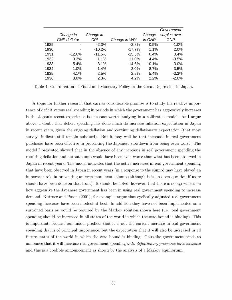
Change in GNP deflator

Change in CPI Change in WPI

Change in GNP

Government surplus over

GNP1929 - -2.3% -2.8% 0.5% -1.0%1930 - -10.2% -17.7% 1.1% 2.0%1931 -12.6% -11.5% -15.5% 0.4% 0.4%1932 3.3% 1.1% 11.0% 4.4% -3.5%1933 5.4% 3.1% 14.6% 10.1% -3.0%1934 -1.0% 1.4% 2.0% 8.7% -3.5%1935 4.1% 2.5% 2.5% 5.4% -3.3%1936 3.0% 2.3% 4.2% 2.2% -2.0%

Table 4: Coordination of Fiscal and Monetary Policy in the Great Depression in Japan.

A topic for further research that carries considerable promise is to study the relative impor-

tance of deficit versus real spending in periods in which the government has aggressively increases

both. Japan’s recent experience is one case worth studying in a calibrated model. As I argue

above, I doubt that deficit spending has done much do increase inflation expectation in Japan

in recent years, given the ongoing deflation and continuing deflationary expectation (that most

surveys indicate still remain subdued). But it may well be that increases in real government

purchases have been effective in preventing the Japanese slowdown from being even worse. The

model I presented showed that in the absence of any increases in real government spending the

resulting deflation and output slump would have been even worse than what has been observed in

Japan in recent years. The model indicates that the active increases in real government spending

that have been observed in Japan in recent years (in a response to the slump) may have played an

important role in preventing an even more acute slump (although it is an open question if more

should have been done on that front). It should be noted, however, that there is no agreement on

how aggressive the Japanese government has been in using real government spending to increase

demand. Kuttner and Posen (2001), for example, argue that cyclically adjusted real government

spending increases have been modest at best. In addition they have not been implemented on a

sustained basis as would be required by the Markov solution shown here (i.e. real government

spending should be increased in all states of the world in which the zero bound is binding). This

is important, because our model predicts that it is not the current increase in real government

spending that is of principal importance, but the expectation that it will also be increased in all

future states of the world in which the zero bound is binding. Thus the government needs to

announce that it will increase real government spending until deflationary pressures have subsided

and this is a credible announcement as shown by the analysis of a Markov equilibrium.

35

7 Conclusion

Inflation has been considered the main threat to monetary stability for several decades. In the

aftermath of the double digit inflation of the 70’s, there was a movement to separate monetary

policy from fiscal policy and vest it in the hands of “independent” central bankers whose primary

responsibility was to prevent inflation. This development was reinforced by important contri-

butions on the theoretical level, most notably by Kydland/Prescott (1977) and Barro/Gordon’s

(1983) illustration of the “inflation bias” of a discretionary government. It is easy to forget that

in the aftermath of the Great Depression, when deflation was the norm, the discussion at the

political and theoretical level was quite the opposite. Paul Samuelson claimed that the Federal

Reserve was “the prisoner of its own independence” during the Great Depression, exaggerating

the slump by its inability to fight deflation.24 Similarly Milton Friedman claimed that “monetary

policy is much too serious a matter to be left to the central bankers".25 This paper shows that

in a deflationary situation there may be some benefit to fiscal and monetary coordination. The

exact nature of this coordination is certainly an interesting topic of further research. It is worth

pointing out that this paper’s solution suggests that it may only need to be temporary to be

effective, as the solution illustrated that the coordination solution converges to the same one that

would result in the absence of coordination.

One may argue that the central bank could, without any coordination with the treasury, engage

in various activities to stimulate the prices and output, such as purchasing foreign exchange or

private assets. An independent central bank may use its own balance sheet to achieve a similar

commitment to higher future prices as was illustrated for deficit spending under coordination

in this paper (i.e. it can increase inflation expectation by open market operations in private

assets or foreign exchange see e.g. Eggertsson (2006) and Svensson and Jeanne (2004) for further

discussion). The idea is that an independent central bank is typically very concerned about the

value of its balance sheet since it would need to finance any capital losses by either printing

money (which may lead inflation than higher than is optimal) or a bailout from the treasury (that

may lead to loss of independence).The snag is, however, that if the bank is too concerned about

its own balance sheet it may find itself as "the prisoner of its own independence" that prevents

it from taking these actions, even if they in principle allow it to commit it to future inflation,

much as suggested by Paul Samuelson. The reason is that any asset bought in a non-standard

open market operations has uncertain returns, and there are always some states of the world in

which the central bank may need to trade-off excessive balance sheet losses to excessive inflation.

Thus even if one considers additional policy instruments there may still be an persuasive case for

temporary coordination of monetary and fiscal policy.

24See Mayer, Thomas (1990) p. 6.25Although he suggested rules to solve the problem rather than coordinated discretion as I do here.

36

8 References

1. Adam and Billi (2006), "Optimal Monetary Policy under Commitment with a Zero Bound

on Nominal Interest Rates", Journal of Money, Credit, and Banking, forthcoming.

2. Adam and Billi (2006), "Discretionary Monetary Policy and the Zero Lower Bound on

Nominal Interest Rates," Journal of Monetary Economics, forthcoming.

3. Albanesi, Christiano, and Chari (2003), "Expectation Traps and Monetary Policy," Review

of Economic Studies, Vol. 70, p. 715-741

4. Auerbach, Allan, and Obstfeld, Maury (2003), "The Case for Open Market Operations,"

working paper, Berkeley.

5. Bernanke, Ben S. (2000), ”Japanese Monetary Policy: A Case of Self-Induced Paralysis?”

in Ryoichi Mikitani and Adam S. Posen, eds., Japan’s Financial Crisis and its Parallels to

the U.S. Experience, Institute for International Economics.

6. Bernanke, Ben S. (2003), "Some Thoughts on Monetary Policy in Japan," Before the Japan

Society of Monetary Economics, May 2003.

7. Barro, Robert J. (1979), ”On the Determination of the Public Debt,” The Journal of Political

Economy, Volume 87, Issue 5, 940-971.

8. Barro, Robert J., Gordon, David B. (1983), ”A Positive Theory of Monetary Policy in a

Natural Rate Model,” The Journal of Political Economy, Volume 91, Issue 4, 589-610.

9. Benhabib, Jess, Stephania Schmitt-Grohe and Martion Uribe (2002) “Avoiding Liquidity

Traps,” Journal of Political Economy, 110, 535-563.

10. Brown, E. Cary, "Fiscal Policy in the ’Thirties: A Reappraisal," American Economic Re-

view, Vol. 46, No.3, p. 857-879.

11. Buiter, Willem H. (2003), ”Deflation: Prevention and Cure,” working paper 9623.

12. Calvo, Guillermo (1983), "Staggered Prices in a Utility-Maximizing Framework," Journal

of Monetary Economics, 12: 383-98.

13. Cargill, Thomas F.(2001), ”Monetary Policy, Deflation, and Economic History: Lessons for

the Bank of Japan,” Monetary and Economic Studies 19(S-1), 113-142.

14. Clause, James, Dale Henderson, Athanasios Orphanides, David Small and Peter Tinsley

(2000), ”Monetary Policy When the Nominal Short-Term Interest Rate is Zero,” Working

Paper.

37

15. Dedola, Luca, "Optimal Monetary Policy under Discretion", Bank of Italy, mimeo.

16. Dixit, A. and Lambertini, L. (2003), "Interaction of commitment and discretion in monetary

and fiscal policies," American Economic Review, 93(5).

17. Eggertsson, Gauti and Woodford, Michael (2003), "The Zero Bound on Interest Rates and

Optimal Monetary Policy," Brookings Papers on Economic Activity 1, 212-219.

18. Eggertsson, Gauti (2005), "Great Expectations and the End of the Depression," NYFed

Staff Report Number 234.

19. Eggertsson, Gauti (2006), "The Deflation Bias and Committing the Being Irresponsible,"

Federal Reserve Bank of New York, mimeo.

20. Eggertsson, Gauti, and Ostry, Jonathan (2005), "Does Excess Liquidity Pose a Threat in

Japan?" IMF Policy Discussion Paper PDP/05/05.

21. Friedman, Milton (1962), ”Capitalism and Freedom,” Chicago, The University of Chicago

Press.

22. Friedman, Milton (1968), ”The Role of Monetary Policy,” American Economic Review, Vol.

58, No1 p. 1-17.

23. Friedman, Milton (1969), ”The Optimum Quantity of Money,” in The Optimum Quantity

of Money and

24. Other Essays, Chicago: Aldine, 1969.

25. Friedman, Milton and Rose (1980), ”Free to choose: a personal statement,” New York,

Harcourt Brace Jovanovich.

26. Fujiki, H., Okina, K., and Shiratsuka, S. (2001), ”Monetary Policy under Zero Interest Rate:

Viewpoints of Central Bank Economists,” Monetary and Economic Studies, Vol. 19, No.

1., 89-131.

27. Fuhrer, Jeffrey C, and Brian Madigan (1997), ”Monetary Policy When Interest Rates are

Bounded at Zero,” Review of Economics and Statistics, November 1997, 79, 573-85..

28. Gertler, Mark (2003), "Commentary on The Zero Bound on Interest Rates and Optimal

Monetary Policy," Brookings Papers on Economic Activity 1, 212-219.

29. Jung, Taehun, Yuki Teranishi, and Tsutomu Watanabe (2006). “Zero Bound on Nominal

Interest Rates and Optimal Monetary Policy,” Journal of Money, Credit, and Banking,

forthcoming.

38

30. Keynes, John Maynard (1936), The General Theory of Employment Interest and Money,

London: Macmillan.

31. King and Plosser (1985), ”Money, Deficits, and Inflation”, Carnegie-Rochester Conference

Series on Public Policy, 22 (Spring): 147-196.

32. Klein, Paul, Krussel, Per and Rios-Rull, Victor. (2003), "Time-Consistent Public Expendi-

tures," mimeo.

33. Krugman, Paul (1998), ”It’s Baaack! Japan’s Slump and the return of the Liquidity Trap,”

Brookings Papers on Economic Activity 2:1998.

34. Krugman, Paul (2001), ”The Fear Economy,” New York Times Sunday Magazine, October.

35. Kuttner, Ken and Posen, Alan (2001), "The Great Recession: Lesson for Macroeconomic

Policy from Japan," Brookings Papers on Economic Activity 2:2001.

36. Kydland, Finn E. and Edward C. Prescott (1977): ”Rules Rather than Discretion: The

Inconsistency of Optimal Plans.” J.P.E. (85): 473-91.

37. Levin, Andrew (1990), ”Monetary Stabilization Policy in a General Equilibrium Model with

Wage Contracts,” mimeo, University of California, San Diego.

38. Lucas, Robert and Stokey, Nancy (1983), ”Optimal Fiscal and Monetary Policy in an Econ-

omy without Capital,” Journal of Monetary Economics 12, p55-93.

39. Lucas, Robert and Stokey, Nancy (1987), ”Money and Interest in a Cash-in-Advance Econ-

omy,” Econometrica; 55(3), May 1987, pages 491-513.

40. Mayer, Thomas (1990), ”The Political Economy of American Monetary Policy,” New York:

Cambridge University Press, 1990.

41. McCallum, Bennett T., ”Theoretical Analysis Regarding a Zero Lower Bound on Nominal

Interest Rates,” working paper, Carnegie Mellon University, 1999.

42. Meltzer, Allan H. ”Comments: What More Can the Bank of Japan Do?”, Monetary and

Economic Studies, 17 (3), Institute for Monetary and Economic Studies, Bank of Japan,

1999, pp. 189-191.

43. Nakamura, Takafusa (1971), ”Economic Growth in Prewar Japan,” Yale University Press.

44. Nakov, Anton (2005), "Optimal and Simple Monetary Policy Rules with Zero Floor on the

Nominal Interest Rate," mimeo.

39

45. Nanto, Dick K., Takagi, Shinji, ”Korekiyo Takahashi and Japan’s Recovery from the Great

Depression,” The American Economic Review Papers and Proceedings, May 1985, Vol. 75

No.2.

46. Obstfeld, M. (1991): ”A Model of Currency Depriciation and the Debt-Inflation Spiral,”

Journal of Economic Dynamics and Control 15, 151-177.

47. Obstfeld, M. (1997): ”Dynamic Seigniorage Theory”, Macroeconomic Dynamics, 1, 1997,

588-614.

48. Patrick, Hugh T (1971) ”The Economic Muddle of the 1920’s” in Dilemmas of Growth in

Prewar Japan, Morley, James (ed), Princeton University Press.

49. Phelps, E.S. (1967), ”Phillips Curves, Expectational Inflation and Optimal Unemployment

over Time,” Economica 2, 22-44.

50. Rogoff, Kenneth (1985),”The Optimal Degree of Commitment to an Intermediate Monetary

Target,” Quarterly Journal of Economics 100, 1169-1189.

51. Rogoff, Kenneth (1998), "Commentary on It’s Baaack! Japan’s Slump and the return of

the Liquidity Trap,” Brookings Papers on Economic Activity 2:1998

52. Sargent, Thomas andWallace, N. (1981) "Some Unpleasant Monetarist Arithmetic," Federal

Reserve Bank of Minneapolis Quarterly Review, 5:3, 1-17.

53. Sims, Christopher A. (1994), ”A Simple Model for the Study of the Determination of the

Price Level and the Interaction of Monetary and Fiscal Policy,” Economic Theory 4: 381-

399.

54. Summers, Lawrence (1991), ”Panel Discussion: Price Stability. how Should Long-Term

Monetary Policy Be Determined?” Journal of Money, Credit and Banking, 23(3), 625-631.

55. Summers, Lawrence (1998), "Emerging from Crisis: The Beginnings of a New Asia." Speech

presentaed to the Economic Stragey Institute, Washington, February 11.

56. Svensson, Lars (1999), ”How Should Monetary Policy Be Conducted in an Era of Price

Stability?” in ”New Challenges for Monetary Policy,” symposium organized by the Federal

Reserve Bank of Kansas City.

57. Svensson, Lars (2001), ”The Zero Bound in an Open-Economy: A Foolproof Way of Escaping

from a Liquidity Trap,” Monetary and Economic Studies 19(S-1), 277-312.

40

58. Svensson, Lars and Jeanne, Olivier (2004), "Credible Commitment to Optimal Escape from

a Liquidity Trap: The Role of the Balance Sheet of an Independent Central Bank", January

2004.

59. Taylor, John B. (1980), ”Aggregate Dynamics and Staggered Contracts”, Journal of Political

Economy, 88(1), 1-23.

60. Woodford, Michael (1994), ”Monetary Policy and Price Level Determinacy in a Cash-in-

Advance Economy.” Economic Theory, 4, 345-380.

61. Woodford, Michael (1996), ”Control of the Public Debt: A Requirement for Price Stabil-

ity?,” NBER working paper No. 5684.

62. Woodford, Michael (2003), "Interest and Prices: Foundations of a Theory of Monetary

Policy", Princeton University.

63. Wolman, Alexander (1999), ”Real Implications of the Zero Bound on Nominal Interest

Rates,” unpublished, Federal Reserve Bank of Richmond.

64. Reifschneider, David, and John C. Williams (2000), ”Three Lessons for Monetary Policy in

a Low Inflation Era,” unpublished, Federal Reserve Board.

41

−5 0 5 10 15 20 25−15

−10

−5

0

inflation

−5 0 5 10 15 20 25

−15

−10

−5

0

output gap

Figure 1: A Markov equilibrium in the absence of active fiscal policy.

−5 0 5 10 15 20 25

−10

−5

0

inflation

−5 0 5 10 15 20 25−15

−10

−5

0

output gap

−5 0 5 10 15 20 25

0

2

4

6real government spending

Figure 2: A Markov equilibrium when the government uses discretionary real spending.

42

−5 0 5 10 15 20 25−1

−0.5

0

0.5

1inflation

−5 0 5 10 15 20 25−3

−2

−1

0

1

2output gap

Figure 3: A Markov equilibrium for inflation and the output gap when the government uses

discretionary deficit spending.

−5 0 5 10 15 20 25−15

−10

−5

0

5

10deficit spending/GDP

−5 0 5 10 15 20 250

20

40

60

debt

Figure 4: A Markov equilibrium for deficit spending and nominal debt when the government uses

discretionary deficit spending.

43

−5 0 5 10 15 20 25−5

−4

−3

−2

−1

0

1inflation

−5 0 5 10 15 20 25

−4

−2

0

2output gap

Figure 5: Comparison of inflation and the output gap in Markov equilibrium when the government

only utilizes discretionary real spending (dashed line), only uses discretionary deficit spending

(dotted line) and when it takes advantage of both (solid line).

−5 0 5 10 15 20 25−15

−10

−5

0

5

10deficit spending/GDP

−5 0 5 10 15 20 25−1

0

1

2

3

4

5government real spending/GDP

Figure 6: Comparison of deficit spending and debt in Markov equilibrium when the government

only utilizes discretionary real spending (dashed line), only uses discretionary deficit spending

(dotted line) and when it takes advantage of both (solid line).

44

i = 0 i > 00

2

4

6

8Real Spending

Multi

plie

r

RBCNK

i = 0 i > 00

2

4

6

8

Multi

plie

rDeficit Spending

Figure 7: Multiplier Effects Under Real and Deficit Spending

.

45

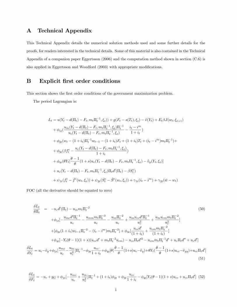
A Technical Appendix

This Technical Appendix details the numerical solution methods used and some further details for the

proofs, for readers interested in the technical details. Some of this material is also contained in the Technical

Appendix of a companion paper Eggertsson (2006) and the computation method shown in section (C.6) is

also applied in Eggertsson and Woodford (2003) with appropriate modifications.

B Explicit first order conditions

This section shows the first order conditions of the government maximization problem.

The period Lagrangian is:

Lt = u(Yt − d(Πt)− Ft,mtΠ−1t , ξt)) + g(Ft − s(Tt), ξt)− v(Yt) +EtβJ(wt, ξt+1)

+ φ1t(um(Yt − d(Πt)− Ft,mtΠ

−1t , ξt)Π

−1t

uc(Yt − d(Πt)− Ft,mtΠ−1t , ξt)

− it − im

1 + it)

+ φ2t(wt − (1 + it)Π−1t wt−1 − (1 + it)Ft + (1 + it)Tt + (it − im)mtΠ

−1t )+

+ φ3t(βfet −

uc(Yt − d(Πt)− Ft,mtΠ−1t , ξt)

1 + it)

+ φ4t(θYt[θ − 1θ(1 + s)uc(Yt − d(Πt)− Ft,mtΠ

−1t , ξt)− vy(Yt, ξt)]

+ uc(Yt − d(Πt)− Ft,mtΠ−1t , ξt)Πtd

0(Πt)− βSet )

+ ψ1t(fet − fe(wt, ξt)) + ψ2t(S

et − Se(wt, ξt)) + γ1t(it − im) + γ2t(w − wt)

FOC (all the derivative should be equated to zero)

δLtδΠt

= −ucd0(Πt)− ummtΠ−2t (50)

+φ1t[−umcd

0Π−1tuc

− ummmtΠ−3t

uc− umΠ

−2t

uc+

umuccd0Π−1t

u2c+

umucmmtΠ−2t

u2c]

+[φ2t(1 + it)wt−1Π−2t − (it − im)mtΠ

−2t ] + φ3t[

uccd0

(1 + it)+

ucmmtΠ−2t

(1 + it)]

+φ4t[−Yt(θ − 1)(1 + s)(uccd0 +mtΠ

−2t ucm)− uccΠtd

02 − ucmmtΠ−1t d0 + ucΠtd

00 + ucd0]

δLtδYt

= uc−vy+φ1t[umc

uc−umu2c]Π−1t −φ3t

ucc1 + it

+φ4t[θ(θ − 1θ(1+s)uc−vy)+θYt(

θ − 1θ(1+s)ucc−vyy)+uccΠtd0]

(51)

δLtδFt

= −uc+ gG+φ1t[−umc

uc+umu2c]Π−1t +(1+ it)φ2t+φ3t

ucc1 + it

−φ4t[Yt(θ− 1)(1+ s)ucc+uccΠtd0] (52)

i

δLtδit

= −φ1t1 + im

(1 + it)2+ φ2t(mtΠ

−1t + Tt − wt−1Π

−1t − F ) + φ3t

uc(1 + it)2

+ γ1t (53)

δLtδmt

= umΠ−1t +φ1t[

umm

uc−umu2c

ucmΠ−1t ]Π−1t +φ2t(it−im)Π−1t −φ3t

ucm1 + it

Π−1t −φ4t[Yt(θ−1)(1+s)ucmΠ−1t −ucmd0]

(54)δLtδTt

= −gGs0(Tt) + φ2t(1 + it) (55)

δLtδwt

= βEtJw(wt, ξt+1)− ψ1tfew − ψ2tS

ew + φ2t − γ2t (56)

δLtδfet

= βφ3t + ψ1t (57)

δLtδSet

= −βφ4t + ψ2t (58)

The complementary slackness conditions are:

γ1t ≥ 0, it ≥ im, γ1t(it − im) = 0 (59)

γ2t ≥ 0, w − wt ≥ 0, γ2t( w − wt) = 0 (60)

The optimal plan under discretion also satisfies an envelope condition:

Jw(wt−1, ξt) = −φ2t(1 + it)Π−1t (61)

Necessary and sufficient condition for a Markov equilibrium thus are given by the first order conditions

(50) to (61) along with the constraints (8), (18), (21), (23) and the definitions (20) and (22). Note that the

first order conditions imply restrictions on the unknown vector function Λt and the expectation functions.

C Approximation Method

This section show the approximation method used to approximate the Markov equilibrium.

C.1 Equilibrium in the absence of seigniorage revenues

As discussed in the text it simplifies the discussion to assume that the equilibrium base money small, i.e.

that mt is a small number (see Woodford (2003), chapter 2, for a detailed treatment). This simplifies the

algebra and my presentation of the results. I discuss in the footnote some reasons for why I conjecture

that this abstraction has no significant effect.26

26First, as shown by Woodford (2003), for a realistic calibration parameters, this abstraction has trivial effect

on the AS and the IS equation under normal circustances. Furthermore, at zero nominal interest rate, increasing

ii

To analyze an equilibrium with a small monetary base I parameterize the utility function by the

parameter m and assume that the preferences are of the form:

u(Ct,mtΠ−1t , ξt) = u(Ct, ξt) + χ(

mt

mΠ−1t C−1t , ξt) (62)

As the parameter m approaches zero the equilibrium value of mt approaches zero as well. At the same

time it is possible for the value of um to be a nontrivial positive number, so that money demand is well

defined and the government’s control over the short-term nominal interest rate is still well defined (see

discussion in the proofs of Propositions 5 in section D). I can define mt =mt

m as the policy instrument of

the government, and this quantity can be positive even as m and mt approach zero. Note that even as the

real monetary base approaches the cashless limit the growth rate of the nominal stock of money associated

with different equilibria is still well defined. I can then still discuss the implied path of money supply for

different policy options. To see this note that

mt

mt−1=

Mt

Pt−1m

Mt−1Pt−2m

=Mt

Mt−1Π−1t−1 (63)

which is independent of the size of m. For a given equilibrium path of inflation and mt I can infer the

growth rate of the nominal stock of money that is required to implement this equilibrium by the money

demand equation. By assuming m→ 0 I only abstract from the effect this adjustment has on the marginal

utility of consumption and seigniorage revenues, both of which would be trivial in a realistic calibration

(see footnote 26).

C.2 Steady state discussion and relation to literature on Markov Equilibrium

In general a steady-state of a Markov equilibrium is non-trivial to compute, as emphasized by Klein et al

(2003). This is because each of the steady state variables depend on the mapping between the endogenous

state (i.e. debt) and the unknown functions J(.) and e(.), so that one needs to know the derivative of

these functions with respect to the endogenous policy state variable to calculate the steady state. Klein

money balances further does nothing to facilitate transactions since consumer are already satiated in liquidity. This

was one of the key insights of Eggertsson and Woodford (2003), which showed that at zero nominal interest rate

increasing money supply has no effect if expectations about future money supply do not change. It is thus of

even less interest to consider this additional channel for monetary policy at zero nominal interest rates than if the

short-term nominal interest rate was positive. Second, assuming mt is a very small number is likely to change the

government budget constraint very little in a realistic calibration. By assuming the cashless limit I am assuming no

seignorage revenues so that the term it−im1+it

mtΠ−1t in the budget constraint has no effect on the equilibrium. Given

the low level of seignorage revenues in industrialized countries I do not think this is a bad assumption. Furthermore,

in the case the bound on the interest rate is binding, this term is zero, making it of even less interest when the zero

bound is binding than under normal circumstances.

iii

et al suggest an approximation method by which one may approximate this steady state numerically by

using perturbation methods. In this paper I take a different approach. Proposition 5 shows that a steady

state may be calculated under assumptions that are fairly common in the monetary literature, without any

further assumptions about the unknown functions J(.) and e(.).

Proposition 5 If ξ = 0 at all times and (i)-(iii) in A4 hold there is a Markov equilibrium steady state that

is given by i = 1/β−1, w = Se = φ1 = φ3 = φ4 = ψ1 = ψ2 = γ1 = γ2 = 0, Π = 1, φ2 = gG(F−s(F ))s0(F ),

fe = uc(Y ), F = F = G = T + s(T ) and Y = Y where Y and F are the unique solution to the equations:

uc(Y − F ) = vy(Y ) and uc(Y − F ) + gG(F − s(F ))s0(F ) = gG(F − s(F ))

To proof the proposition about the steady state I look at the algebraic expressions of the first order

conditions of the government maximization problem. The proof is in section (D). A noteworthy feature

of the proof is that the mapping between the endogenous state and the functions J(.) and e(.) does not

matter (i.e. the derivatives of these functions cancel out). The reason is that the Lagrangian multipliers

associated with the expectation functions are zero in steady state and I may use the envelope condition to

substitute for the derivative of the value function. The intuition for why these Lagrangian multipliers are

zero in equilibrium is simple. At the steady state the distortions associated with monopolistic competition

are zero (because of A2 (ii)). This implies that there is no gain of increasing output from steady state.

In the steady the real debt is zero and according to assumption (i) seigniorage revenues are zero as well.

This implies that even if there is cost of taxation in the steady state, increasing inflation does not reduce

taxes. It follows that all the Lagrangian multipliers are zero in the steady state apart from the one on the

government budget constraint. That multiplier, i.e. φ2, is positive because there are steady state tax costs.

Hence it would be beneficial (in terms of utility) to relax this constraint.

There is by now a rich literature studying the question whether there can be multiple Markov equilibria

in monetary models that are similar in many respects to the one I have described here (see e.g. Albanesi et

al (2003), Dedola (2002) and King and Wolman (2003)). I do not proof the global uniqueness of the steady

state in Proposition 5 but show that it is locally unique.27 I conjecture, however, that the steady state

is globally unique under A2.28 But even if I would have written the model so that it had more than one

27See Woodford (2003) Appendix A3 for definition and discussion of local uniqueness in stochastic general equi-

librium models of this kind.28The reason for this conjecture is that in this model, as opposed to Albanesi et al and Dedola work, I assume

in A2 that there are no monetary frictions. The source of the multiple equilibria in those papers, however, is the

payment technology they assume. The key difference between the present model and that of King and Wolman, on

the other hand, is that they assume that some firms set prices at different points in time. I assume a representative

iv

steady state, the one studied here would still be the one of principal interest as discussed in the footnote.29

C.3 Approximate system and order of accuracy

The conditions that characterize equilibrium are given by the constraints of the model and the first order

conditions of the governments problem. A linearization of this system is complicated by the Kuhn-Tucker

inequalities (59) and (60). I look for a solution in which the bound on government debt is never binding,

and then verify that this bound is never binding in the equilibrium I calculate. Under this conjectured the

solution to the inequalities (59) and (60) can be simplified into two cases:

Case 1 : γ1t = 0 if it > im (64)

Case 2 : it = im otherwise (65)

Thus in both Case 1 and 2 I have equalities characterizing equilibrium. These equations are (9), (18),(19),

(21), (23), (24), (20), (22) and (50)-(58) and either (64) when it > im or (65) otherwise. Under the

condition A1(i) and A1(ii) but im < 1β − 1 then it > im and Case 1 applies in the absence of shocks. In

the knife edge case when im = 1β − 1,however, the equations that solve the two cases (in the absence of

shocks) are identical since then both γ1t = 0 and it = im. Thus both Case 1 and Case 2 have the same

steady state in the knife edge case it = im. If I linearize around this steady state (which I show exists in

Proposition 5) I obtain a solution that is accurate up to a residual (||ξ||2) for both Case 1 and Case 2. As

a result I have one set of linear equations when the bound is binding, and another set of equations when it

firm, thus abstacting from the main channel they emphasize in generating multiple equilibria. Finally the present

model is different from all the papers cited above in that I introduce nominal debt as a state variable. Even if the

model I have illustrated above would be augmented to incorporate additional elements such as montary frictions

and staggering prices, I conjecture that the steady state would remain unique due to the ability of the government

to use nominal debt to change its future inflation incentive. That is, however, a topic for future reasearch and there

is work in progress by Eggertsson and Swanson that studies this question.29Even if I had written a model in which the equilibria proofed above is not the unique global equilibria the

one I illustrate here would still be the one of principal interest. Furthermore a local analysis would still be useful.

The reason is twofold. First, the equilibria analyzed is identical to the commitment equilibrium (in the absence of

shocks) and is thus a natural candidate for investigation. But even more importantly the work of Albanesi et al

(2002) indicates that if there are non-trivial monetary frictions there are in general only two steady states.There are

also two steady states in King and Wolman’s model. (In Dedola’s model there are three steady states, but the same

point applies.) The first is a low inflation equilibria (analogues to the one in Proposition 1) and the other is a high

inflation equilibria which they calibrate to be associated with double digit inflation. In the high inflation equilibria,

however, the zero bound is very unlikely ever to be binding as a result of real shocks of the type I consider in this

paper (since in this equilibria the nominal interest rate is very high as I will show in the next section). And it is

the distortions created by the zero bound that are the central focus of this paper, and thus even if the model had

a high inflation steady state, that equilibria would be of little interest in the context of the zero bound.

v

is not. The challenge, then, is to find a solution method that, for a given stochastic process for ξt, finds

in which states of the world the interest rate bound is binding and the equilibrium has to satisfy the linear

equations of Case 1, and in which states of the world it is not binding and the equilibrium has to satisfy

the linear equations in Case 2. Since each of these solution are accurate to a residual (||ξ||2) the solutions

can be made arbitrarily accurate by reducing the amplitude of the shocks. The next subsection show a

solution method, assuming as simple process for the natural rate of interest, that numerically calculates

when Case 1 applies and when Case 2 applies.

Note that I may also consider solutions when im is below the steady state nominal interest rate. A linear

approximation of the equations around the steady state in Proposition 5 is still valid if the opportunity

cost of holding money, i.e. δ ≡ (i− im)/(1+ i), is small enough. Specifically, the result will be exact up to

a residual of order (||ξ, δ||2). In the numerical example in the text I suppose that im = 0 (see Eggertsson

and Woodford (2003) for further discussion about the accuracy of this approach when the zero bound is

binding). A nontrivial complication of approximating the Markov equilibrium is that I do not know the

unknown expectation functions e(.). I illustrate a simple way of matching coefficients to approximate this

function in section (C.5).

C.4 Linearized solution

I here linearize the first order conditions and the constraints around the steady state in Propositions 5. I

assume the form of the utility discussed in section C.1. I allow for deviations in the vector of shocks ξt and

in im so that the equations are accurate of order o(||ξ, δ||2). I abstract from the effect of the shocks on the

disutility of labor. Here dzt = zt − zss The economic constraints are:

ucd00dΠt + θ(ucc − vyy)dYt + θucξdξt − ucd

00βEtdΠt+1 = 0 (66)

uccdYt + ucξdξt − βuccEtdYt+1 − βucξEtdξt+1 − βucdit + βucEtdΠt+1 = 0 (67)

dwt −1

βdwt−1 +

1

βdTt = 0 (68)

dSet − ucd00EtdΠt+1 = 0 (69)

dfet + ucEtdΠt+1 − uccEtdYt+1 − ucξEtξt+1 = 0 (70)

The equation determining the natural rate of output is:

(vyy − ucc)dYnt + (vyξ − ucξ)dξt −

(θ − 1)θ

ucds = 0 (71)

vi

The equation determining the natural rate of interest is:

βEt(uccdYnt+1 − ucξEtdξt+1)− (uccdY n

t − ucξdξt) + βuccdrnt = 0 (72)

Note that the real money balances deflated by m, i.e. mt, are well defined in the cashless limit so that

equation 63 is

dmt − dmt−1 − dMt

Mt−1+ dπt−1 = 0

and money demand is approximated by

χmm

ucdmt −

χmm

ucmdΠt −

χmm

ucmdYt − βdit + βdim = 0

The Kuhn Tucker conditions imply that

Case 1 when it > im

dγ1t = 0 (73)

Case 2 when it = im

dit = 0 (74)

I look for a solution in which case the debt limit is never binding so that dγ2t = 0 at all times and verify

that this is satisfied in equilibrium. Linearized FOC in a Markov Equilibrium

−d00ucdΠt + φ2β−1dwt−1 + d00ucdφ4t = 0 (75)

(ucc − vyy)dYt + ucξdξt − vyξdξt − uccβdφ3t + θ(ucc − vyy)dφ4t = 0 (76)

−uccdYt + uccd0dΠt + (ucc + gGG)dFt + (gGG − ucc)dξt − gGGs

0dTt (77)

+(1 + ı)dφ2t + φ2dit +ucc1 + ı

dφ3t − [Y (θ − 1)(1 + s)ucc + uccd0]dφ4t = 0

φ2dTt − φ2dwt−1 + ucβ2dφ3t + dγ1t = 0 (78)

gGG(s0)2dTt − gGs

00dTt − gGξdξt + β−1dφ2t + φ2dit = 0 (79)

dφ2t −Etdφ2t+1 − βφ2Etdit+1 + φ2EtdΠt+1 + βfwdφ3t − βSwdφ4t − dγ2t = 0 (80)

Note that the first order condition with respect to mt does not play any role in the cashless limit so that

it is omitted above. Also note that the two derivatives fw and Sw are in general not known. In the next

section I show how these derivatives can be found

vii

C.5 Approximating fw and Sw

I show how the two derivatives fw and Sw can be approximated under A5. At time t ≥ τ the system is

deterministic. Then I can approximate these functions to yield wt = w1wt−1 and dΛt = Λ1wt−1, where

the first element of the vector dΛt is dπt = π1wt−1, the second dYt = Y 1wt−1 and so on and wt = w1wt−1

where the vector Λ1 and the number w1 are some unknown constants. To find the value of each of these

coefficients I substitute this solution into the system (66)-(70) and (75)-(80) and match coefficients. For

example equation (66) implies that

ucd00π1wt−1 + θ(ucc − vyy)Y

1wt−1 − ucd00βπ1w1wt−1 = 0 (81)

where I have substituted for dπt = π1wt−1 and for dπt+1 = π1wt = π1w1wt−1. Note that I assume that

t ≥ τ so that there is perfect foresight and I may ignore the expectation symbol. This equation implies

that the coefficients π1, y1 and w1 must satisfy the equation:

ucd00π1 + θ(ucc − vyy)Y

1 − ucd00βπ1w1 = 0 (82)

I may similarly substitute the solution into each of the equation (66)-(70) and (75)-(80) to obtain a system

of equation that the coefficients must satisfy:

ucd00π1 + θ(ucc − vyy)Y

1 − ucd00βπ1w1 = 0 (83)

uccY1 − βuccY

1w1 − βuci1 + βucπ

1w1 = 0 (84)

w1 − 1β+1

βT 1 = 0 (85)

S1 − ucd00π1w1 = 0 (86)

f1 + ucπ1w1 − uccY

1w1 = 0 (87)

−djucπ1 +s0gGβ

+ d00ucφ14 = 0 (88)

(ucc − vyy)Y1 − uccβφ

13 + θ(ucc − vyy)φ

14 = 0 (89)

s0gGT1 − s0gG + ucβ

2φ13 = 0 (90)

gGG(s0)2T 1 − gGs

00T 1 + β−1φ12 + gGs0i1 = 0 (91)

φ12 − φ12w1 − βgGs

0i1w1 + gGs0π1w1 + βf1φ13 − βS1φ14 = 0 (92)

There are 11 unknown coefficients in this system i.e. π1, Y 1, i1, F 1, S1, f1, T 1, φ12, φ13, φ

14, w

1. For a given

value of w1, (83)-(91) is a linear system of 10 equations with 10 unknowns, and thus there is a unique

viii

value given for each of the coefficients as long as the system is non-singular (which can be verified to be the

case for standard functional forms for the utility and technology functions). The value of w1 is in general

not unique, but in the calibrated model there is always a unique bounded solution in the examples I have

studied (and the unbounded solutions will violate the debt limit). In a simplified version of the model it

can be proofed that there is a unique solution for w1 that satisfies all the necessary conditions, but I have

not managed to proof it in this model (see discussion in Eggertsson (2006)).

C.6 Computational method

Here I illustrate a solution method for the optimal commitment solution. This method can also be applied,

with appropriate modification of each of the steps, to find the Markov solution. I assume shocks so that

the natural rate of interest becomes unexpectedly negative in period 0 and the reverts back to normal with

probability αt in every period t as in A5 (one may use (71) and (72) to find what a given negative number

for the natural rate of interest implies for the underlying exogenous shocks). I assume that there is a final

date K in which the natural rate becomes positive with probability one (this date can be arbitrarily far

into the future).

The solution takes the form:

Case 2 it = 0 ∀ t 0 ≤ t < τ + k

Case 1 it > 0 ∀ t t ≥ τ + k

Here τ is he stochastic date at which the natural rate of interest returns to steady state. I assume that

τ can take any value between 1 and the terminal date K that can be arbitrarily far into the future. The

number τ + kτ is the period in which the zero bound stops being binding in the contingency when the

natural rate of interest becomes positive in period τ . Note that the value of kτ can depend on the value of

τ . I first show the solution for the problem as if I knew the sequence kτSτ=1. I then describe a numerical

method to find the sequence kτSτ=1.

C.6.1 The solution for t ≥ τ + kτ

The system of linearized equations (75)-(80), (66)-(70), and (73) can be written in the form:⎡⎢⎣ EtZt+1

Pt

⎤⎥⎦ =M

⎡⎢⎣ Zt

Pt−1

⎤⎥⎦

ix

where Zt ≡∙Λt et φt ψt γ1t

¸Tand Pt ≡ wt. If there are fifteen eigenvalues of the matrix M outside

the unit circle this system has a unique bounded solution of the form:

Pt = Ω0Pt−1 (93)

Zt = Λ0Pt−1 (94)

C.6.2 The solution for τ ≤ t < τ + k

Again this is a perfect foresight solution but with the zero bound binding. The solution now satisfies the

equations (75)-(80), (66)-(70) but (74) instead of (73).The system can be written on the form:⎡⎢⎣ Pt

Zt

⎤⎥⎦ =⎡⎢⎣ A B

C D

⎤⎥⎦⎡⎢⎣ Pt−1

Zt+1

⎤⎥⎦+⎡⎢⎣ M

V

⎤⎥⎦This system has a solution of the form:

Pτ+j = Ωkτ−jPτ+j−1 +Φ

kτ−j (95)

Zτ+j = Λkτ−jPτ+j−1 +Θ

kτ−j (96)

where j = 0, 1, 2, ..., k. Here Ωkτ−j is the coefficient in the solution when there are kτ − j periods until

the zero bound stops being binding (i.e. when j − kτ = 0 the zero bound is not binding anymore and the

solution is equivalent to (93)-(94)). We can find the numbers Λj ,Ωj ,Θj and Φj for j = 1, 2, 3, ....., k by

solving the equations below using the initial conditions Φ0 = Θ0 = 0 for j = 0 and the initial conditions

for Λj and Ωj given in (93)-(94):

Ωj = [I −BΛj−1]−1A

Λj = C +DΛj−1Ωj

Φj = (I −BΛj−1)−1[BΘj−1 +M ]

Θj = DΛj−1Φj +DΘj−1 + V

C.6.3 The solution for t < τ

The solution satisfies (75)-(80), (66)-(70), and (74). Note that each of the expectation variables can be

written as xt = Etxt+1 = αt+1xt+1 + (1 − αt+1)xt+1 where αt+1 is the probability that the natural

rate of interest becomes positive in period t + 1. Here hat on the variables refers to the value of each

x

variable contingent on that the natural rate of interest is negative. I may now use the solution for Zt+1

in 96 to substitute for Zt+1, i.e. the value of each variable contingent on that the natural rate becomes

positive again, in terms of the hatted variables. The value of xt+1, for example, can be written as xt+1 =

Λkt+121 φ1t+Λ

kt+122 φ2t+Θ

kt+12 where Λkt+1ij is the ijth element of the matrix Λkt+1 and the value kt+1 depends

on the number of additional periods that the zero bound is binding (recall that I am solving the equilibrium

on the assumption that I know the value of the sequence kτSτ=1) . Hence I can write the system as:⎡⎢⎣ Pt

Zt

⎤⎥⎦ =⎡⎢⎣ At Bt

Ct Dt

⎤⎥⎦⎡⎢⎣ Pt−1

Zt+1

⎤⎥⎦+⎡⎢⎣ Mt

Vt

⎤⎥⎦I can solve this backwards from the dateK in which the natural rate returns back to normal with probability

one. I can then calculate the path for each variable to date 0. Note that.

BK−1 = DK−1 = 0

By recursive substitution I can find a solution of the form:

Pt = ΩtPt−1 +Φt (97)

Zt = ΛtPt−1 +Θt (98)

where the coefficients are time dependent. To find the numbers Λt,Ωt,Θt and Φt consider the solution of

the system in period K − 1 when BK−1 = DK−1 = 0. I have:

ΩK−1 = AK−1

ΦK−1 =MK−1

ΛK−1 = CK−1

ΘK−1 = VK−1

I can find of numbers Λt,Ωt,Θt and Φt for period 0 to K− 2 by solving the system below (using the initial

conditions shown above for S − 1):

Ωt = [I −BtΛt+1]−1At

Λt = Ct +DtΛt+1Ωt

Φt = (I −BtΛt+1)−1[BtΘt+1 +Mt]

Θt = DtΛt+1Φt +DtΘt+1 + Vt

xi

Using the initial condition P−1 = 0 I can solve for each of the endogenous variables under the contingency

that the trap last to period K by (97) and (98). I then use the solution from (93)-(96) to solve for each of

the variables when the natural rate reverts back to steady state.

C.6.4 Solving for kτ∞t=0

A simple way to find the value for kτ∞τ=1 is to first assume that kτ is the same for all τ and find the k so

that the zero bound is never violated. Suppose that the system has converged at t = 25 (i.e. the response

of each of the variables is the same). Then I can move to 24 and see if kτ = 4 for τ = 1, 2, ...24 is a solution

that never violates the zero bound. If not move to 23 and try the same thing and so on. For preparing this

paper I wrote a routine in MATLAB that applied this method to find the optimal solution and verified

that the results satisfied all the necessary conditions. It turned out that in the Markov equilibrium the zero

bound stopped being binding as soon as the natural rate of interest is positive again (the same is not true

for the commitment equilibrium as shown in Eggertsson (2006) and Eggertsson and Woodford (2003)).

C.7 Calibration for numerical results

In the numerical examples I assume the following functional forms for preferences and technology:

u(C, ξ) =C1−σ

−1C σ−1

1− σ−1

where C is a preference shock assumed to be 1 in steady state.

g(G, ξ) = g1G1−σ

−1Gσ−1

1− σ−1

where G is a preference shock assumed to be 1 in steady state

v(H, ξ) =λ1

1 + λ2H1+λ2H−λ2

where H is a preference shock assumed to be 1 in steady state

y = Ah

where A is a technology shock assumed to be 1 in steady state. I may substitute the production function

into the disutility of working to obtain (assuming A=1):

v(Y, ξt) =λ11 + ω

Y 1+ωH−λ2

When calibrating the shocks that generate the temporarily negative natural rate of interest I assume that

it is the shock C that is driving the natural rate of interest negative (as opposed to A) since otherwise a

xii

negative natural rate of interest would be associated with a higher natural rate of output which does not

seem to be the most economically interesting case. I assume that the shock G is such that the Ft would be

constant in the absence of the zero bound, in order to keep the optimal size of the government (in absence

of the zero bound) constant as discussed in the text. The cost of price adjustment is assumed to take the

form:

d(Π) = d1Π2

The cost of taxes is assumed to take to form:

s(T ) = s1T2

Aggregate demand impliesY = C +F = C +G+ s(F ). I normalize Y = 1 in steady state and assume that

the share of the government in production is F = 0.3. Tax collection as a share of government spending is

assumed to be γ = 5% of government spending. This implies

0.05 =s(F )

F= s1F

so that s1 =γF . The result for the inflation and output gap response are not very sensitive to varying

γ under either commitment or discretion. The size of the public debt issued in the Markov equilibrium,

however, crucially depends on this variable. In particular if γ is reduced the size of the debt issued rises

substantially. For example if γ = 0.5% the public debt issued is about ten times bigger than reported in

the figure in the paper. I assume that government spending are set at their optimal level in steady state

as discussed in the text:

g2 =uc

gG − s0gG=

C−σ−1

G−σ−1(1− s0)

= (G

C)σ−1 1

1− s0= (

G

C)σ−1 1

1− 2s1F

The IS equation and the AS equation are

xt = Etxt+1 − σ(it −Etπt+1 − rnt )

πt = kπt + βEtπt+1

I assume, as Eggertsson and Woodford, that the interest rate elasticity, σ, is 0.5. The relationship between

σ and σ is

σ = σY

C

I assume that κ is 0.02 as in Eggertsson and Woodford (2003). The relationship between κ and the other

parameters of the model is κ = θ (σ−1+λ2)d00 . I scale hours worked so that Y = 1 in steady state which implies

xiii

vy = λ1 and using the uc = vy one obtains λ1 = 1.Finally I assume that θ = 7.87 as in Rotemberg and

Woodford and that ω = 2. For a linear production function ω is the inverse of the Frisch elasticity of labor

supply. The calibration value for the parameters are summarized in the table below:

Table 5

σ 0.71

g1 1.11

λ1 1

ω 2

d1 787

s1 0.17

θ 7.87

D Proofs

D.1 Proof of Proposition 5

Proposition 5 If ξ = 0 at all times and (i)-(iii) in A4 hold there is a Markov equilibrium steady state

that is given by i = 1/β − 1, w = Se = φ1 = φ3 = φ4 = ψ1 = ψ2 = γ1 = γ2 = 0, Π = 1, φ2 =

gG(F − s(F ))s0(F ), fe = uc(Y ), F = F = G = T + s(T ) and Y = Y where Y and F are the unique

solution to the equations: uc(Y − F ) = vy(Y ) and uc(Y − F ) + gG(F − s(F ))s0(F ) = gG(F − s(F ))

I only proof existence of this steady state here but do not discuss uniqueness (see Eggertsson (2006)

for discussion about uniqueness of a Markov equilibrium in this model). In the assumption made in the

proposition I assume the cashless limit and the form of the utility:

u(Ct,mtΠ−1t , ξt) = u(Ct, ξt) + χ(

mt

mΠ−1t C−1t , ξt) (99)

The partial derivatives with respect to each variable are given by

uc = uc − χ0m

mC−2Π−1 (100)

um =χ0

mC−1Π−1 (101)

umm =χ00

m2C−2Π−2 < 0 (102)

ucm = −χ00m

m2C−3Π−2 − χ0

mC−2Π−1 (103)

xiv

As m− > 0 I assume that for m = mm > 0 I have

limm→0χ0m≡ χ0 ≥ 0 (104)

limm→0χ00m2≡ χ00 > 0 (105)

This implies that there is a well defined money demand function, even as money held in equilibrium

approaches zero, given byχ0(mC−1t Π

−1t , ξt)C

−1t Π

−1t

uc(Ct, ξt)=

it − im

1 + it

so that χ0 = 0 when it = imt . From the assumptions (104)-(105) it follows that:

limm→0χ0 = 0

limm→0χ00 = 0

Then the derivatives uc and ucm in the cashless limit are:

limm→0

uc = uc

and

limm→0

ucm = limm→0

[−m χ00m2

m

mC−3Π−1 − χ0

mC−2] = −χ0C−2

Hence in a steady state in which m→ 0 and it = im I have that χ0 = 0 so that at the steady state

limm→0

ucm = 0. (106)

Note that this does not imply that the satiation point of holding real balances is independent of consump-

tion. To see this note that the satiation point of real money balances is is given by some finite number

S∗ = mmY which implies that χ(S ≥ S∗) = v(S∗). The value of the satiation point as m→ 0 is:

limm→0S∗ ≡ S = mC

The value of this number still depends on C even as m→ 0 and even if ucm = 0 at the satiation point.

I now show that the steady state stated in Proposition 3 satisfies all the first order conditions and the

constraints. The steady state candidate solution in is:

i =1

β− 1, w = φ1 = φ3 = φ4 = ψ1 = ψ2 = γ1 = γ2 = 0,Π = 1, φ2 = gGs

0, T = F (107)

xv

and Y and F are the unique solution to the equations stated in the proposition. Note that (107) and

the functional assumption about d imply that:

d0 = 0 (108)

Let us first consider the constraints. In the steady state the AS equation is

θY [θ − 1θ(1 + s)uc − vy]− ucΠd

0(Π) + βucΠd0(Π) = 0

Since by (108) d’=0, and according to assumption (ii) of the propositions θ−1θ (1 + s) = 1 the AS equation

is only satisfied in the candidate solution if

uc = vy (109)

Evaluated in the candidate solution the IS equation is:

1

1 + i=

βucucΠ−1 = β

which is always satisfied at because it simply states that i = 1 − 1/β which is consistent with the steady

state I propose in the propositions and assumption (iii). The budget constraint is:

w − (1 + i)Π−1w − (1 + i)F + (1 + i)T + (1 + i)mmΠ−1t = 0

which is also always satisfied in our candidate solution since it states that F = T , w = 0 and m→ 0. The

money demand equation indicates that the candidate solutions is satisfied if

um = Πuci− im

1 + i= 0 (110)

By (20) and (22) the expectation variables in steady state are

Se = ucΠd0

fe = ucΠ

Since Π = 1 and d0 = 0 by (108) these equations are satisfied in the candidate solution. Finally both the

inequalities (9) and (19) are satisfied since w > w = 0 in the candidate solution and i = im.

I now show that the first order conditions, i.e. the commitment and the Markov equilibrium first order

conditions, that are given by (50)-(61), are also consistent with the steady state suggested.

I start with (50). It is

xvi

−ucd0 − ummmΠ−2 + φ1[−umcd

0Π−1

uc− ummmmΠ−3

uc− umΠ

−2

uc+

umuccd0Π−1

u2c+

umucmmmΠ−2

u2c](111)

+[φ2(1 + i)wΠ−2 − (i− im)mmΠ−2] + φ3[uccd

0

1 + i+

ucmmmΠ−2

(1 + i)]

+φ4[−Y (θ − 1)(1 + s)(uccd0 + mmΠ−2ucm)− uccΠd

02 − ucmmmΠ−1d0 + ucΠd00 + ucd

0]

By (108) and (110) the first two terms are zero. The constraints that are multiplied by φ1, φ3, φ4, ψ1 and

ψ2 are also zero because each of these variables are zero in our candidate solution (107). Finally, the term

that is multiplied by φ2 (which is positive) is also zero because w = 0 in our candidate solution (107) and

so is i− im. Thus I have shown that the candidate solution (107) satisfies (50).

Let us now turn to (51). It is

uc− vy+φ1[umc

uc− um

u2c]Π−1−φ3

ucc1 + i

+φ4[θ(θ − 1θ(1+s)uc− vy)−θY (

θ − 1θ(1+s)ucc− vyy)−uccΠd0] = 0

(112)

The first two terms uc − vy are equal to zero by (109). The next terms are also all zero because they are

multiplied by the terms φ1, φ3, φ4, ψ1 and ψ2 which are all zero in our candidate solution (107). Hence

this equation is also satisfied in our candidate solution. Let us then consider (53). It is:

−φ11 + im

(1 + i)2+ φ2(mm+ T − wΠ−1 − F ) + φ3

uc(1 + i)2

+ γ1 = 0

Again this equation is satisfied in our candidate solution because φ1 = φ3 = w = 0, F = T and m→ 0 in

the candidate solution. Conditions (54) in steady state is:

mmumΠ−1+φ1[

umm

uc− um

u2cucmΠ

−1]+φ2(i−im)mm−φ3ucm1 + i

Π−1−φ4[Y (θ−1)(1+s)ucmΠ−1−ucmd0] = 0

(113)

The first term is zero by (110). All the other terms are also zero because φ1, φ3, φ4, ψ1 and ψ2 are all zero

in our candidate solution (107). Finally i = im in our candidate solution so that the third term is zero as

well. Conditions (55)and (52) in steady state are:

−gGs0(T ) + φ2(1 + i) = 0 (114)

−uc + gG + φ1t[−umc

uc+

umu2c]Π−1t + (1 + i)φ2 + φ3t

ucc1 + it

− φ4t[θYt(θ − 1θ(1 + s)ucc + uccΠtd

0] (115)

Using our candidate solution (107) I obtain:

uc(Y − F ) = gG(F − s0(F )) + gGs0(F )

xvii

which along with (109) is the equation that determine Y and F that was stated in the propositions 3 and

4. Using our assumption on s and standard Inada boundary conditions one may show that these equations

have unique solution for Y and F .

Let us now turn to (56). This equation involves three unknown functions, Jw, few and Sew.I can use

(61) to substitute for Jw obtaining

−βφ2(1 + i)Π−1 − ψ1βfew − ψ2βS

ew + φ2 − γ2 = 0 (116)

In general I cannot know if this equation is satisfied without making further assumption about few and Sew.

But note that in my candidate solution ψ1 = ψ2 = 0. Thus the terms involving these two derivatives in

this equation are zero. Since γ2 = 0, this equation is satisfied if (1 + i)Π−1 = 1/β. This is indeed the case

in our candidate solution. Finally (57) and (58) are satisfied since φ3 = φ4 = ψ1 = ψ2 = 0 in the candidate

solution. Thus I have shown that all the necessary and sufficient conditions of a Markov equilibrium are

satisfied by our candidate solution (107). QED

D.2 Proof of Proposition 3 and 4

Proposition 3 The power of real government spending does not depend on policy coordination, i.e. equi-

librium B in diagram 2 (equation (48) holds) does not depend on whether or not the central bank is

goal independent.

The proof is simple but tedious. The central bank takes Ft = Tt as exogenously given and its maxi-

mization problem can be characterized by the Lagrangian:

Lt = (Πt − 1)2 + λx(Yt − Y nt )

2

+ φ1t(um(Yt − d(Πt)− Ft,mtΠ

−1t , ξt)Π

−1t

uc(Yt − d(Πt)− Ft,mtΠ−1t , ξt)

− it − im

1 + it)

+ φ2t(wt − (1 + it)Π−1t wt−1 − (1 + it)Ft + (1 + it)Tt + (it − im)mtΠ

−1t )

+ φ3t(βfet −

uc(Yt − d(Πt)− Ft,mtΠ−1t , ξt)

1 + it)

+ φ4t(θYt[θ − 1θ(1 + s)uc(Yt − d(Πt)− Ft,mtΠ

−1t , ξt)− vy(Yt, ξt)]

+ uc(Yt − d(Πt)− Ft,mtΠ−1t , ξt)Πtd

0(Πt)− βSet )

+ ψ1t(fet − fe(ξt)) + ψ2t(S

et − Se(ξt)) + γ1t(it − im)

taking Ft as given.

xviii

The treasury takes mt as exogenously given and its maximization problem is:

Lt = u(Yt − d(Πt)− Ft,mtΠ−1t , ξt)) + g(Ft − s(Tt), ξt)− v(Yt)

+ φ1t(um(Yt − d(Πt)− Ft,mtΠ

−1t , ξt)Π

−1t

uc(Yt − d(Πt)− Ft,mtΠ−1t , ξt)

− it − im

1 + it)

+ φ2t(wt − (1 + it)Π−1t wt−1 − (1 + it)Ft + (1 + it)Tt + (it − im)mtΠ

−1t )+

+ φ3t(βfet −

uc(Yt − d(Πt)− Ft,mtΠ−1t , ξt)

1 + it)

+ φ4t(θYt[θ − 1θ(1 + s)uc(Yt − d(Πt)− Ft,mtΠ

−1t , ξt)− vy(Yt, ξt)]

+ uc(Yt − d(Πt)− Ft,mtΠ−1t , ξt)Πtd

0(Πt)− βSet ) + γ1t(it − im)

+ γ2t(w − wt)

The proof is obtained by writing the first order condition of each of these maximization problems, linearizing

them around the steady state in Proposition 3 and showing that the resulting equilibrium conditions are

identical to the equilibrium conditions under coordination (detailed derivation is available upon request).

Proposition 4 If the central bank is goal independent deficit spending has no effect, i.e. in equilibrium

C in diagram 2 (equation (49) holds) deficit spending has no effect on inflation, output or interest

rates when the central bank is goal independent .

The proof here is similar to the last proof and a little tedious. The central bank takes Tt = T (wt−1, ξ)

as exogenously given and its maximization problem can be characterized by the Lagrangian:

Lt = (Πt − 1)2 + λx(Yt − Y nt )

2

+ φ1t(um(Yt − d(Πt)− Ft,mtΠ

−1t , ξt)Π

−1t

uc(Yt − d(Πt)− Ft,mtΠ−1t , ξt)

− it − im

1 + it)

+ φ2t(wt − (1 + it)Π−1t wt−1 − (1 + it)Ft + (1 + it)Tt + (it − im)mtΠ

−1t )

+ φ3t(βfet −

uc(Yt − d(Πt)− Ft,mtΠ−1t , ξt)

1 + it)

+ φ4t(θYt[θ − 1θ(1 + s)uc(Yt − d(Πt)− Ft,mtΠ

−1t , ξt)− vy(Yt, ξt)]

+ uc(Yt − d(Πt)− Ft,mtΠ−1t , ξt)Πtd

0(Πt)− βSet )

+ ψ1t(fet − fe(ξt)) + ψ2t(S

et − Se(ξt)) + γ1t(it − im)

xix

taking T (wt−1, ξ) as given.

The treasury takes mt as exogenously given and its maximization problem is:

Lt = u(Yt − d(Πt)− Ft,mtΠ−1t , ξt)) + g(Ft − s(Tt), ξt)− v(Yt)

+ φ1t(um(Yt − d(Πt)− Ft,mtΠ

−1t , ξt)Π

−1t

uc(Yt − d(Πt)− Ft,mtΠ−1t , ξt)

− it − im

1 + it)

+ φ2t(wt − (1 + it)Π−1t wt−1 − (1 + it)Ft + (1 + it)Tt + (it − im)mtΠ

−1t )+

+ φ3t(βfet −

uc(Yt − d(Πt)− Ft,mtΠ−1t , ξt)

1 + it)

+ φ4t(θYt[θ − 1θ(1 + s)uc(Yt − d(Πt)− Ft,mtΠ

−1t , ξt)− vy(Yt, ξt)]

+ uc(Yt − d(Πt)− Ft,mtΠ−1t , ξt)Πtd

0(Πt)− βSet )

+ γ2t(w − wt)

The proof is obtained by writing the first order condition of each of these maximization problems, linearizing

them around the steady state in Proposition 3 and showing that the resulting equilibrium conditions of the

central bank are identical to the first order conditions of the government when there is no deficit spending.

These conditions are sufficient to characterize the solution for output, inflation and interest rates. The

first order conditions for the treasury then determine the equilibrium path for taxes and debt (detailed

derivation is available upon request)..

xx