Fiscal Policy Multipliers in a New KeynesianModel under Positive and Zero Nominal

Interest Rate�

Lorant Kaszaby

Cardi¤ Business School

April 25, 2011

AbstractThis paper uses a simple new-Keynesian model (with and without capital) and cal-

culates multipliers of four types. That is, we assume either an increase in governmentspending or a cut in sales/labor/capital tax that is �nanced by lump-sum taxes (Ri-cardian evidence holds). We argue that multipliers of a temporary �scal stimulus forseparable preferences and zero nominal interest rate results in lower values than whatis obtained by Eggertsson (2010). Using Christiano et al. (2009) non-separable utilityframework which they used to calculate spending multipliers we study tax cuts as welland �nd that sales tax cut multiplier can be well above one (joint with governmentspending) when zero lower bound on nominal interest binds. In case of a permanentstimulus we show in the model without capital and assuming non-separable preferencesthat it is the spending and wage tax cut which produce the highest multipliers withvalues lower than one. In the model with capital and assuming that the nominal rate is�xed for a one-year (or two-year) duration we present an impact multiplier of govern-ment spending that is very close to the one in Bernstein and Romer (2009) but laterdeclines with horizon in contrast to their �nding and in line with the one of Cogan et al.(2010). We also demonstrate that the long-run spending multiplier calculated similarlyto Campolmi et al. (2010) implies roughly the same value for both types of preferencesfor particular calibrations. For comparison, we also provide long-run multipliers usingthe method proposed by Uhlig (2010).

JEL codes: E45Keywords: New-Keynesian model, �scal multipliers, zero lower bound, monetary

policy, government spending, tax cut, permanent, transitory.

�This paper is a revised and extended version of my Masters thesis from Central European Universitywith the same title. I thank for the comments received at Cardi¤ Business School PhD seminar in October2010.

yCardi¤ Business School, Cardi¤ University, Colum Drive, Cardi¤, CF10 3EU, UK.Email: kaszabl@cardi¤.ac.uk

1

1 Introduction

The American Recovery and Reinvestment Act was passed at the beginning of 2009 in order

to help the US economy recover from the �nancial crises started in 2008. Bernstein and

Romer (2009) provided a document that gives a detailed picture of the estimated e¤ects of

this stimulus package1. However, there is wide disagreement in the economics profession on

the value of the �scal multipliers2 listed in their paper3. As Cogan et al. (2009) assert, it is not

straightforward what kind of model Bernstein and Romer (2009) used to obtain multipliers

above one4 for a permanent increase in government spending under the assumption that the

nominal interest rate is held constant5 for the time interval of their simulation. Furthermore,

Cogan et al. (2009) argues that the Bernstein and Romer (2009) model can�t be a New

Keynesian model as the model�s setup would imply explosive dynamics.

This paper proposes a standard New Keynesian dynamic stochatic general equilibrium

(DSGE) model (with and without capital) used widely in academic literature and in central

banks for supporting decision-making to investigate into the e¤ects of various �scal stimuli

on output both for zero and non-zero nominal interest rate. The DSGE model used here is

basically a stochastic growth (or RBC) model enriched with monopolistic competition on the

product market and staggered price setting in Calvo-style (Calvo, 1983). Being aware that

�scal policy is not constrained to variations only in spending but can also operate with various

taxes to achieve its goal, we consider three possible sources of a �scal stimulus separately:

an increase in non-productive (that is not creating investment opportunities in the economy)

government spending, a sales tax cut and a cut in payroll tax.

Of course, this is not the �rst paper using a New Keynesian model that studies �scal

multipliers. Two recent contributions of the topic are Christiano et al. (2010) and Eggertsson

(2010). Christiano et al. (2010) discuss government spending both for a model with and

without capital when the zero bound on interest rate is binding and not-binding by using

non-separable preferences in consumption and leisure. Their most interesting �nding is that

the spending multiplier is more than three times higher when the nominal interest rate is

zero compared to the case when it is positive. Eggertsson (2010) calculates �scal multipliers

(payroll tax cut, pro�t tax cut, sales tax cut, capital tax cut and an increase in government

1For example, in their Table 5, they provide numbers on the jobs created in each industry in 2010Q4 asa result of the Recovery Package.

2This is the change in output due to a change in government spending, dYt+k=dGt: For k = 0 we get backthe impact multiplier.

3In particular, in their Appendix 1 they consider "output e¤ects of a permanent stimulus of 1% of GDP(percent)"

4That is, a dollar spent by the government increases output by more than one dollar.5Note that the federal funds rate at the time of the introduction of the recovery package was almost zero

and this is a fact that a model has to take into consideration.

2

spending) for the case of separable preferences with special attention to the case of binding

zero bound on nominal interest rate. His most interesting �nding is that the multiplier

associated with a payroll tax cut is negative.

In this paper we argue that the multipliers associated with a temporary �scal stimulus

using separable preferences and assuming that the nominal interest rate is zero are lower than

the same ones calculated by Eggertsson (2010)6. Moreover, we show by using non-separable

preferences that we can obtain multipliers of magnitude similar to the ones in Eggertsson

(2010) when interest is zero. Our model is based on the one by Christiano et al. (2010).

However, we extend the model of Christiano et al. (2010)� who restrict the analysis to

government spending in their models without capital� by taxes of three types.

Furthermore, we check the robustness of the �ndings of a permanent �scal stimulus by

Eggertsson (2010)� who uses separable utility� for non-separable utility and conclude that

the long-run multipliers (when the Taylor rule is in action and nominal interest rate is allowed

to be positive) associated with a permanent stimulus can be of somewhat higher magnitude

than the ones reported by him. In particular, we found that a permanent rise spending or a

permanent labour tax cut lead to a positive multiplier that is much smaller than one.

After extending the new-Keynesian model with capital we emphasize three more �ndings.

Firstly, the di¤erence between separable and non-separable preferences concerning the sizeof the multiplier diminishes on impact� that is, with certain calibration they are roughly

the same� if we consider long-run multipliers (calculated similarly to the one in Campolmi

et al., 2010). Secondly, we present that the impact multiplier associated with a transitoryand anticipated increase in government spending� under the assumption that utility is non-

separable and the nominal interest is held �xed for two years� is equal to one in line with

Bernstein and Romer (2009). Thirdly, multipliers of longer horizon are de�nitely lower thanthe ones reported by Bernstein and Romer (2009) and somewhat higher than the ones by

Cogan et al. (2010) who, unlike us, assumed permanent stimulus7.

This paper shows by using non-separable preferences that we can match the stylised fact

of rising consumption in response to a positive government spending shock. As it is well-

known, when Ricardian equivalence holds, the use of non-separable preferences mitigates

the negative wealth e¤ect associated with the fact that consumers expect a rise in future

taxes when there is an increase in government spending (or a tax cut) in the present. In the

6The di¤erence between the results of Eggertsson (2010) and ours� with respect to the government spend-ing multiplier� comes from the fact that he assumed zero steady-state government spending (quite unusual tomost of the literature but similar to Woodford (2010)) while we assume a steady-state government spending-output ratio of 20% consistent with most of the post-war experience as discussed by Baxter and King (1993).

7Multipliers from a new-Keynesian model under a permanent stimulus must be lower than the same onesunder a transitory experiment as we show below. That is, it is a question how Bernstein and Romer (2009)obtained numbers higher than ours knowing that we used a transitory stimulus.

3

following we provide some empirical evidence on the weakness of this negative wealth e¤ect

(Monacelli and Perotti, 2008).

There is extensive empirical literature on the e¤ect and size of �scal multipliers (see, e.g.,

Blanchard and Perotti, 2002 and Gali et al., 2007). For example, Gali et al. (2007) reports

some VAR evidence that government spending multiplier i.e. the change in output with re-

spect to a change in government spending, is 0:78 on impact, and 1:74 at the end of the second

year. Interestingly they also found that consumption, working hours and wages respondto increased government purchuses positively in small and large (including a complete listof explanatory variables) VAR models on many subsamples. Is is also important that the

magnitude of the response in consumption, working hours and wages are quantitatively large.

In case of consumption the change is usually close to or larger than one in the 4th and the 8th

quarter but de�nitely not on impact after a rise in government spending. However, not all

the empiricial VAR literature is consistent with the positive connection between consumption

and government spending. For example, the identi�cation strategy applied by Ramey (2008)

implies that shortly after increases in government spending consumption declines. The latter

one is based on capturing news about government spending hikes, instead of relying on the

delayed e¤ect as in standard VAR.

The outline of the thesis is as follows. In Section 2 and 3, we formulate a simple New-

Keynesian model and derive analytical short-run (or impact) multipliers of four cases (for

both separable and non-separable preferences, respectively). In section 4, we modify the

baseline model with separable preferences to investigate into the case of zero nominal interest

rate. Section 5 summarise and discuss multipliers from the models without capital. Next,

in Section 6, we calculate and brie�y assess multipliers of permanent stimuli. Section 7

contains the baseline model augmented with capital to assess the robustness of the �ndings

of the models without capital. Finally, we conclude with the main results.

2 A simple DSGE model without capital

The setup of the model used here builds strongly upon Christiano et al. (2010). The idea of

tax rates (labour, sales and capital tax) are introduced into the model following Eggertsson

(2010). However, Eggertsson (2010) use only separable preferences, while here both sep-arable and non-separable preferences are used and discussed. Christiano et al. (2010) use

non-separable preferences and refers to their results� without reporting them� on separable

preferences. As we will see, the optimality conditions can always be characterised by the in-

tratemporal condition, the intertemporal Euler equation, the New Keynesian Phillips curve

(NKPC), the exogenous shock process and the Taylor rule.

4

2.1 The household�s problem

The household maximises the following utility that is separable in consumption and leisure:

U = E0

1Xt=0

�t�C1��t � 11� � � N

1+'t

1 + '+ v(GNt )

�

with respect to its budget constraint

(1� �At )(1 +Rt)Bt +Z 1

0

profitt(i)di+ (1� �Wt )PtWtNt = Bt+1 + (1 + �St )PtCt + Tt

where �At ; �Wt and �St denote, respectively, tax on capital, labour and consumption. Bt

denotes the amount of one-period riskless bonds, Rt is the net nominal one-period rate of

interest that pays o¤ in period t: Nt is the sum of all labour types i, that is, Nt �R 10Nt(i)di

and PtWtNt denotes the �mass�of nominal wages (with the real wage rate Wt). Tt denotes

lump-sum taxes net of transfers. profiti denotes the pro�t of �rm i. The transversality

condition, limt!1Bt+1= [(1 +R0)(1 +R1):::(1 +Rt)] � 0 , is also satis�ed.The household has separable preferences in consumption (Ct), leisure (1 � Nt) and gov-

ernment spending (v(Gt)). We do not specify v here as it is not needed for the optimality

conditions. Throughout the whole paper we assume that � > 1 and ' � 0:

2.2 The �rms�problem

2.2.1 Final good sector

The competitive �rms produce a single �nal good using the following technology:

Yt =

�Z 1

0

Yt(i)��1�

� ���1

; � > 1

where Yt(i); i 2 [0; 1] denotes the intermediate good i: The pro�t-maximisation problem of

competitive �rms results in the demand equation for Yt(i):

Yt(i) =

�Pt(i)

Pt

���Yt (1)

where Pt(i) denotes the price of the intermediate good i and Pt is the price of the homogenous

�nal good.

5

2.2.2 Intermediary sector

The intermediate good i, Yt(i), is produced by a monopolist ith using a linear technology:

Yt(i) = Nt(i)

where Nt(i) denotes the hours used by monopolist i to produce intermediate good i: To be

able to calculate multipliers analytically, we later abstract from capital formation in this

section. However, in Section 5 we introduce capital into the production function as well. We

assume that there is no entry or exit into the industry that produces the ith intermediate

good. Furthermore, we have Calvo-price setting that means that a random fraction of �rms

are allowed to re-optimise its price every period with probability 1� �: With probability � afraction of �rms cannot re-optimise their price and uses their previous period price:

Pt(i) = Pt�1(i):

The discounted pro�t of the ith intermediary �rm can be written as:

Et

1XT=0

�t+Tvt+T [Pt+T (i)Yt+T (i)� (1� �)Wt+TNt+T (i)] ;

where we assume that the subsidy is set such (� = 1�) that corrects for the steady-state

distortion induced by the presence of monopoly power and vt+T is the Lagrange multiplier

on the budget contraint in the household�s optimisation problem.

2.3 Monetary Policy

The monetary policy is assumed to follow the following simple rule:

Rt+1 = max(Zt+1; 0) (2)

where

Zt+1 = (1=�)(1 + �t)��(1��R)(Yt=Y )

�Y (1��R)[�(1 +Rt)]�R � 1 (3)

where Y denotes the steady-state value of Yt8. �t is the time-t rate of in�ation. As usual,

we assume that �� > 1 and �Y 2 (0; 1): The main implication of the rule in equation (2) isthat whenever the nominal interest rate becomes negative, the monetary policy set it equal

to zero, otherwise it is set by the Taylor rule speci�ed in equation (3). The parameter �R8And for the rest of the paper, a variable without a time subscript denotes steady-state value.

6

measures how quickly monetary policy reacts to changes in in�ation and output and we

assume that 0 < �R < 1. Furthermore, we also assume that the in�ation in steady state is

zero which implies that steady-state net nominal interest rate is 1=� � 1:

2.4 Fiscal policy

We have an exogenous AR(1) process for government spending (and the same could be written

for labour tax and sales tax as well):

Gt+1 = (Gt)�G exp("Gt+1) (4)

where �G measures persistence of government spending process and "G is an i:i:d: shock with

zero mean and constant variance. We assume in this simple model that the government

spending, the labour tax cut, the sales tax cut and the employment subsidy to restore e¢ -

ciency in steady-state is �nanced through lump-sum taxes. That is, the Ricardian equivalence

holds under our assumptions and the exact timing of taxes is irrelevant and we don�t have to

take into consideration the government budget constraint. The implications of �scal policy

when the nominal rate is zero is discussed in Section 4.

2.5 Equilibrium

De�nition 1 A monetary equilibrium is a collection of stochastic processes which contains

endogenously determined quantitites fYt(i); Yt; Nt; Nt(i); Bt+1g, prices fPt(i); Pt; �t;Wt; Rt; vtgand an exogenous process fGtg with initial condition G0. The equilibrium can be charac-

terised by �ve equations which we rewrite for their log-linear form. The Intratemporal, Euler,

NKPC, the shock process and the Taylor equations are listed below together with market

clearing. The real marginal cost that appears in the NKPC coincides with Wt due to the

linear technology (i.e. it is model-speci�c). Variables with a hat,b, denote percentage devia-tions from their steady-states: bNt � log(Nt=N), bCt � log(Ct=C) with the exception of taxesb� it � � it�� i; i = fA; S;Wg, which are already expressed in percentages and bGt which is de�nedas the percentage deviation (Gt �G) from steady-state output9 (Y ): bGt � (Gt �G)=Y . Forin�ation, �t, and nominal interest rate, Rt, we consider their deviation from steady-state.

Intratemporal condition (in linearised form)

dMCt = cWt = ' bNt + � bCt + 1

1� �W b�Wt + 1

1 + �Sb�St

9Thus, a percentage increase in bGt is comparable with the percentage change in output (bYt) because bothvariables start from the same steady-state (Y ).

7

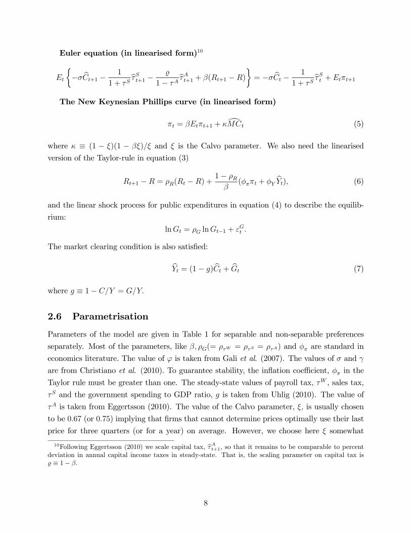
Euler equation (in linearised form)10

Et

��� bCt+1 � 1

1 + �Sb�St+1 � %

1� �Ab�At+1 + �(Rt+1 �R)�= �� bCt � 1

1 + �Sb�St + Et�t+1

The New Keynesian Phillips curve (in linearised form)

�t = �Et�t+1 + �dMCt (5)

where � � (1 � �)(1 � ��)=� and � is the Calvo parameter. We also need the linearisedversion of the Taylor-rule in equation (3)

Rt+1 �R = �R(Rt �R) +1� �R�

(���t + �Y bYt); (6)

and the linear shock process for public expenditures in equation (4) to describe the equilib-

rium:

lnGt = �G lnGt�1 + "Gt :

The market clearing condition is also satis�ed:

bYt = (1� g) bCt + bGt (7)

where g � 1� C=Y = G=Y:

2.6 Parametrisation

Parameters of the model are given in Table 1 for separable and non-separable preferences

separately. Most of the parameters, like �; �G(= ��W = ��S = ��A) and �� are standard in

economics literature. The value of ' is taken from Gali et al. (2007). The values of � and

are from Christiano et al. (2010). To guarantee stability, the in�ation coe¢ cient, �� in the

Taylor rule must be greater than one. The steady-state values of payroll tax, �W , sales tax,

�S and the government spending to GDP ratio, g is taken from Uhlig (2010). The value of

�A is taken from Eggertsson (2010). The value of the Calvo parameter, �; is usually chosen

to be 0:67 (or 0:75) implying that �rms that cannot determine prices optimally use their last

price for three quarters (or for a year) on average. However, we choose here � somewhat

10Following Eggertsson (2010) we scale capital tax, b�At+1, so that it remains to be comparable to percentdeviation in annual capital income taxes in steady-state. That is, the scaling parameter on capital tax is% � 1� �:

8

larger (0:85) for reasons asserted in the following sections11. The standard deviation of the

noise term (�"G ; �"�W , �"�S and �"�A ) of the shock process in equation (4) for all four types

of stimulus is one percent.

Table 1: Parametrisation of the New Keynesian Model without Capital

Parameters Separable Non-separable� 2 2' 0.2 na� 0.99 0.99 na 0.29

�G = ��W = ��S = ��A 0.8 0.8�� 1.5 1.5�Y 0 0�R 0 0� 0.85 0.85

G=Y (� g) 0.18 0.18�W 0.28 0.28�A 0.00 0.00�S 0.05 0.05

�"G = �"�W = �"�S = �"�A 0.01 0.01Implied parameters

� 0.03 0.03N na 1/3

Remark to Table 1: na=non applicable. The parameters' and are applicable for separable and non-separablepreferences, respectively.

2.7 Multipliers for Separable Preferences

There are three important requirements for being able to solve the model analytically by

methods of undetermined coe¢ cients: (1) linear production function, (2) no interest rate

smoothing in Taylor rule (�R = 0) and (3) the assumption that government spending and

changes in distortionary taxes are �nanced through lump-sum taxes (in other words Ricar-

dian equivalence holds). The parametrisation for the separable case can be found in the

�rst column of Table 1. The exact formulas for the multipliers (by assuming that the zero

11The Calvo parameter, �, should be greater than 0:82 for two reasons: (1) we can achieve a governmentspending multiplier that is larger than one for non-separable preferences in the model with positive nominalinterest rate and (2) we can meet the algebraic requirement in the model of Section 4 for the zero bound tobind.

9

bound does not bind in this section) presented here are derived under the above three main

assumptions.

We solve the model analytically by using the method of undetermined coe¢ cients. That

is, we guess that output and in�ation is some function of bGt (and similarly for b�Wt ,b�St andb�At ) and can be expressed as:�t = A� bGt; (8)

bYt = AY bGt: (9)

Moreover, we can eliminate forward-looking variables, like EtGt+1, if we assume an exogenous

AR(1) process for government spending as it is in equation (4).

2.7.1 Multipliers for separable preferences

First, we discuss when the government spending multiplier is larger than one. For this

purpose, take the total derivative of the linear version of the aggregate resource constraint

in equation (7):

dYtdGt

=dbYtd bGt =

dh(1� g) bCt + bGti

d bGt = 1 + (1� g)dbCtd bGt : (10)

This formula implies that the size of the spending multiplier depends on how consumption

reacts to government spending. For separable preferences the latter one in equation (10) is

negative: d bCt=d bGt < 0. Thus, the spending multiplier is smaller than one and this can alsobe seen on Figure 1 where consumption falls and the multiplier is smaller than one on impact

(0:97).

The government spendig, payroll tax cut, sales tax cut and capital tax cut multipliers for

separable preferences are given, respectively, by the following formulas:

dbYtd bGt = �

(1� �) + (1� g)(�� � �) �1���

�(1� �) + �Y (1� g) + (1� g)(�� � �) �1���

�'+ �

1�g

� ;dbYt�db�Wt =

(�� ��) �1���

11��W

� � (�� ��) �1��� ('+ �)� (��� �Y )

;

dbYt�db�St =

11+�S

h(�� 1)� (�� � �) �

1���

i(� + �Y ) + (�� � �) �

1��� ('+ �)� ��;

10

Figure 1: Impulse responses of the simple new-Keynesian model with separable preferencesto a one percent spending shock. We can see that dC=dG < 0:

0 10 200

0.2

0.4

0.6

0.8

1

time

dY/dG

0 10 200

0.05

0.1

0.15

0.2

time

perc

enta

ge d

evia

tion 

from

 st.s

t. Yhat

0 10 200

0.2

0.4

0.6

0.8

1

time

perc

enta

ge d

evia

tion 

from

 st.s

t. Ghat

0 10 200

0.002

0.004

0.006

0.008

0.01

0.012

0.014

time

APR

π

0 10 200

0.005

0.01

0.015

0.02

time

APR

R

0 10 20­7

­6

­5

­4

­3

­2

­1

0x 10 ­3

timepe

rcen

tage

 dev

iatio

n fro

m s

t.st Chat

anddbYt�db�At = �%�

(�Y + �)� �1��� ('+ �) (�� ��)� ��

�(1� �A)

:

As we have discussed it previously the spending multiplier (which is 0:97 under the para-

metrisation used in Table 1) is always smaller than one with separable preferences. It can

be also be noted that with certain parametrisation it can be very close to one but never goes

beyond one. Under baseline parametrisation in Table 1 we assumed that monetary policy

reacts to only in�ation through the Taylor rule (�� > 1; �Y = 0). Instead, we can assume

that the monetary policy reacts to changes in the output gap as well (where �Y can take

the positive value originally proposed by Taylor (1993)). In the latter case the multiplier is

lower than the one under pure in�ation targeting (results for the case when we have positive

coe¢ cient on output gap� in particular it is set to �Y = 0:5=4� can be seen in Table 8 in

Appendix). We discuss these results in the section when we summarise temporary �scal

multipliers.

The value of the labour tax cut multiplier (with the baseline calibration) is 0:23, which is

similar to those found in new-Keynesian literature (see, e.g., Eggertsson (2010)). The reason

11

why this multiplier is lower than the spending and sales tax ones is because it stimulates

output only indirectly through an outward shift in the labour supply.

The value of the sales tax cut multiplier (0:44) is generally lower than the one for govern-

ment spending as this variable has a coe¢ cient ( 11+�S

) in the Euler equation that generally

downscales its value. The baseline idea behind sales tax decrease is that people consume more

goods with a lower tax on them. However, we know that VAT-type taxes (like sales tax) are

comparatively lower in developed countries than in less-developed ones. Thus, the potential

stimulative e¤ects of a huge sales tax decrease may turn out to be small for a country like

the US.

3 Non-separable preferences

The household maximises the following utility that is non-separable in consumption (Ct) and

leisure (1�Nt):

U = E0

1Xt=0

�t

"[C t (1�Nt)1� ]

1�� � 11� �

#with respect to its budget constraint

(1� �A)(1 +Rt)Bt +Z 1

0

profitt(i)di+ (1� �Wt )PtWtNt = Tt +Bt+1 + (1 + �St )PtCt:

3.1 Equilibrium conditions

Again, the equilibrium conditions can be described by the intratemporal condition, the Euler

equation, the new-Keynesian Phillips curve, the Taylor rule and the shock process. We list

only those equilibrium conditions which change after imposing the non-separable preferences

assumption.

The intratemporal condition

cWt = bCt + N

1�NbYt + 1

1� �W b�Wt + 1

1 + �Sb�St ; (11)

where steady-state hours, N , depends on g (or, in case of tax cut multipliers, it depend on

steady-states taxes) and preference parameter, .

12

The Euler equation

Et

�� (Rt+1 �R) + [(1� �) � 1] bCt+1 � (1� )(1� �) N

1�NbNt+1 � 1

1 + �Sb�St+1�

= [(1� �) � 1] bCt � (1� )(1� �) N

1�NbNt � 1

1 + �Sb�St + %

1� �AEtb�At+1 + Et�t+1(12)The New Keynesian Phillips curve, the Taylor rule and the shock process is the same.

In case of non-separable preferences the general form of NKPC is the same as in equation

(5) with only real marginal cost, dMCt, being di¤erent from the one for separable case. Whenusing linear production function the real marginal cost coincides with real wage, dMCt = cWt;

which latter is given the intratemporal condition in equation (11). We also need a Taylor

rule (in equation (6)) and an exogenous shock process (see equation (4)) to close the system.

3.2 The role of non-separable preferences

In the NewKeynesian model used here we have in�nitely-lived agents, complete asset markets,

monopolistic competition, lump-sum taxation and sticky prices. One of our major �nding

is that the size of the government spending multiplier depends largely on the preference

speci�cation of the representative household. In order to generate a government spending

multiplier that is larger than one we have to assume complementarity between consumption

and hours worked, that is, non-separable preferences in consumption and leisure has to be

used.

In the New Keynesian model with separable preferences, a rise in government spending

induce a negative wealth e¤ect as the consumer expects a rise in future lump-sum taxes and,

as a consequence, he/she consumes less and works more. The negative wealth e¤ect implies

an outward shift in the labour supply curve leading to higher hours worked and lower real

wages while the labour demand curve remains unchanged. The negative Hicksian wealth

e¤ect induced by government spending leads to a rise in output and a fall in consumption

and real wages.

However, there is little empirical evidence on the strength of this negative wealth e¤ect

(see, e.g., Gali et al., 2007). Monacelli and Perotti (2008) revisits the so-called Greenwood-

Hercowitz-Hu¤mann (GHH) preferences which implies a very low Hicksian wealth e¤ect and

concludes by using non-separable preferences of GHH type that we can generate a case when

the labour supply curve does not shift, but stays still, in reaction to a rise in government

spending (that is, the wealth e¤ect is zero).

If there was a shift in the labour supply, the real wage would decrease and the consumer

13

would substitute consumption for hours worked (negative substitution e¤ect). Thus, to

generate a rise in consumption we need the real wage to increase that can be only achieved

by a positive outward shift in the labour demand curve. To make this happen we have to

introduce sticky prices into the model. Under the presence of sticky prices, not all the �rms

can change its prices when the demand for their products, due to an increase in government

purchases, increase. Thus, those �rms who cannot change price will satisfy new demand by

an increase in production which can be achieved by hiring extra workers. When hiring extra

workers, labour demand shifts out and the rising real wage as a necessary condition for rising

consumption after a spending spree is satis�ed (Monacelli and Perotti, 2008).

3.3 Multipliers for Non-separable Preferences

It remains true also in case of non-separable preferences that we can solve for the mul-

tipliers (see necessary assumptions at the separable case) analytically by the methods of

undetermined coe¢ cients. Figure 2 shows the response of variables (and the multiplier) to a

temporary 1% spending shock under non-separable preferences. We can observe two things:

(1) the multiplier is slightly larger than one (1:05) on impact and (2) dC=dG > 0:

Figure 2: Impulse responses of the simple new-Keynesian model with non-separable prefer-ences to a one percent spending shock. We can observe that dC=dG > 0:

0 10 200

0.2

0.4

0.6

0.8

1

1.2

1.4

time

dY/dG

0 10 200

0.05

0.1

0.15

0.2

0.25

time

perc

enta

ge d

evia

tion 

from

 st.s

t. Yhat

0 10 200

0.2

0.4

0.6

0.8

1

time

perc

enta

ge d

evia

tion 

from

 st.s

t. Ghat

0 10 200

0.01

0.02

0.03

0.04

0.05

0.06

0.07

time

APR

π

0 10 200

0.02

0.04

0.06

0.08

0.1

time

APR

R

0 10 200

0.005

0.01

0.015

time

perc

enta

ge d

evia

tion 

from

 st.s

t Chat

14

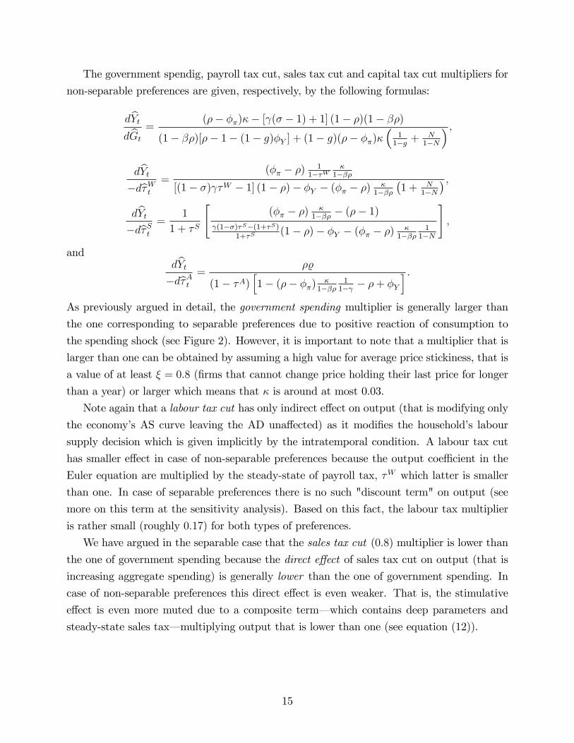
The government spendig, payroll tax cut, sales tax cut and capital tax cut multipliers for

non-separable preferences are given, respectively, by the following formulas:

dbYtd bGt = (�� ��)�� [ (� � 1) + 1] (1� �)(1� ��)

(1� ��)[�� 1� (1� g)�Y ] + (1� g)(�� ��)��

11�g +

N1�N

� ;dbYt�db�Wt =

(�� � �) 11��W

�1���

[(1� �) �W � 1] (1� �)� �Y � (�� � �) �1���

�1 + N

1�N� ;

dbYt�db�St = 1

1 + �S

"(�� � �) �

1��� � (�� 1) (1��)�S�(1+�S)

1+�S(1� �)� �Y � (�� � �) �

1���1

1�N

#;

anddbYt�db�At = �%

(1� �A)h1� (�� ��) �

1���11� � �+ �Y

i :As previously argued in detail, the government spending multiplier is generally larger than

the one corresponding to separable preferences due to positive reaction of consumption to

the spending shock (see Figure 2). However, it is important to note that a multiplier that is

larger than one can be obtained by assuming a high value for average price stickiness, that is

a value of at least � = 0:8 (�rms that cannot change price holding their last price for longer

than a year) or larger which means that � is around at most 0.03.

Note again that a labour tax cut has only indirect e¤ect on output (that is modifying only

the economy�s AS curve leaving the AD una¤ected) as it modi�es the household�s labour

supply decision which is given implicitly by the intratemporal condition. A labour tax cut

has smaller e¤ect in case of non-separable preferences because the output coe¢ cient in the

Euler equation are multiplied by the steady-state of payroll tax, �W which latter is smaller

than one. In case of separable preferences there is no such "discount term" on output (see

more on this term at the sensitivity analysis). Based on this fact, the labour tax multiplier

is rather small (roughly 0:17) for both types of preferences.

We have argued in the separable case that the sales tax cut (0:8) multiplier is lower than

the one of government spending because the direct e¤ect of sales tax cut on output (that is

increasing aggregate spending) is generally lower than the one of government spending. In

case of non-separable preferences this direct e¤ect is even weaker. That is, the stimulative

e¤ect is even more muted due to a composite term� which contains deep parameters and

steady-state sales tax� multiplying output that is lower than one (see equation (12)).

15

4 When zero lower bound on interest rate binds

4.1 The two-state process

In accordance with Christiano et al. (2010) we assume that the zero bound on nominal

interest rate binds due to an exogenous increase in the discount rate (people�s propensity

toward savings increases). To be able to model zero bound we modify the discount factor in

the household�s problem to become time dependent and is given by the cumulative product

of interest rates. Christiano et al. (2010) considers non-separable utility but, now, we

consider the separable case. That is, the household maximises its utility which is separable

in consumption and leisure:

U = E0

1Xt=0

dt

"C1��t � 11� � +

(1�Nt)1+'

1 + '

#

with respect to its budget constraint:

(1� �A)(1+Rt)Bt+Z 1

0

profitt(i)di+(1� �Wt )Z 1

0

PtWt(i)Nt(i)di = Tt+Bt+1+(1+ �St )PtCt

where the discount factor, dt is given by (rt+1 denotes the real rate of interest at time t that

will be actual in t+ 1).

The time-varying discount factor is given by:

dt =

(1

1+r11

1+r2::: 11+rt

; t � 11; t = 0:

Initially the economy is in the steady-state. Then, in the �rst period r1 = rl. Then, for t � 1;rt evolves as follows. The discount factor remains high with probability p:

Pr(rt+1 = rljrt = rl) = p:

Or, the discount factor jump back to its steady-state value with probability 1� p:

Pr(rt+1 = rjrt = rl) = 1� p:

We assumed that initially we are in the zero bound and thus:

Pr(rt+1 = rljrt = r) = 0:

16

In period 0 < t � T zero bound binds while in period t > T zero bound ceases to bind. Weassume that the shock to the discount factor is high enough to make the zero bound binding.

Moreover the following holds in steady-state (the steady-state value of rt+1 is denoted as r):

�(1 + r) = 1. When zero bound binds in�ation, output and government spending at time t

is denoted by �l, bYl, and bGl respectively.In period t and t+ 1 variable bXi = f bGi; bYi; �ig; for i 2 ft; t+ 1g are taking, respectively,

the following values:

bXt =

( bXt = bXl; 0 < t � T , zero bound binding,bXt = 0; t > T , zero bound not binding,

and

bXt+1 =

((1� p) bXt = 0; with probab. 1� p variable X reverts back to steady-state,

p bXl; with probab. p zero bound continues to bind.

In summary, the relevant cases are: bGt = bGl; Et( bGt+1) = p bGl; Et(�t+1) = p�l; bYt = bYl; andEt(bYt+1) = pbYl:4.2 Solution and calibration of the model

The equilibrium is characterised by two values for each variable: one value when the zero

bound binds and one when it does not. When zero bound binds output and in�ation are

given, respectively, by the following closed form equations:

bYl = ��(p� 1)(1� �p)� �p�

� bGl+

�(1� g) [(1� �p)(p� 1) + p�]

(1 + �S)

�b�Sl (13)

+(1� g)(1� �p)%(1� �A) b�Al + (1� g)(1� �p)

�rl

+(1� g)p�(1� �W )b�Wl

17

and

�l =� ('(1� g) + �)(1� �p)(1� g)

�f�(p� 1)(1� �p)� �p�g ('(1� g) + �)� ��

('(1� g) + �)

� bGl+� ('(1� g) + �)(1� �p)(1� g)

�(1� g) [(1� �p)(p� 1) + p�] (1� �p) + �

(1 + �S)

�b�Sl+� ('(1� g) + �) %(1� �p)(1� �A)b�Al (14)

+� ('(1� g) + �)

�rl

+

�('(1 + g) + �) p�2 + �

(1� �p)(1� �W )

�b�Wlwith � �(1� p)(1� �p)� p�('(1� g) + �). The algebraic requirement for the zero lowerbound to bind is > 0, which is satis�ed, ceteris paribus, for 0:028 � � � 0:0465 (or,

equivalently, 0:81 � � � 0:85). That is the Calvo parameter, �, should be su¢ ciently large.

Why does the zero bound bind in equilibrium?Christiano et al. (2010) has an appealing interpretation for market clearing when zero

bound binds. In this simple model without investment the savings has to be zero in equi-

librium. A possible way to curb peoples�desire to save more is through a reduction in the

real interest rate. According to the Fisher rule we know there are two possible ways to de-

crease real interest rate: a decrease in the nominal rate or an increase in expected in�ation.

However, we know that the decrease in the nominal rate is limited by its natural zero lower

bound. We also know that the in�ation cannot accelerate when there is a discount factor

shock (if we look at equation (14), and, at the same time, assuming that �scal variables do

not change, we can see there is de�ation due to rl < 0). Otherwise, positive in�ation in

our sticky prices model is accompanied by increasing output that can induce people to save

more. Thus, the reduction in real interest rate may not be enough to deter people from

further saving. If the discount rate shock is big enough the real interest rate cannot fall by

enough to reduce savings because the zero bound becomes binding prior to the point that

would re-establish equilibrium. Therefore, the only possible way for savings to become zero

in equilibrium is a large transitory fall in output and an accompanying de�ation as it canbe seen on the element (1,2) and (1,3) of Figure 3, respectively.

The government spending multiplier when the zero bound binds is given by the coe¢ cient

on bGl in equation (13) as:dbYld bGl = �(p� 1)(1� �p)� �p�

:

18

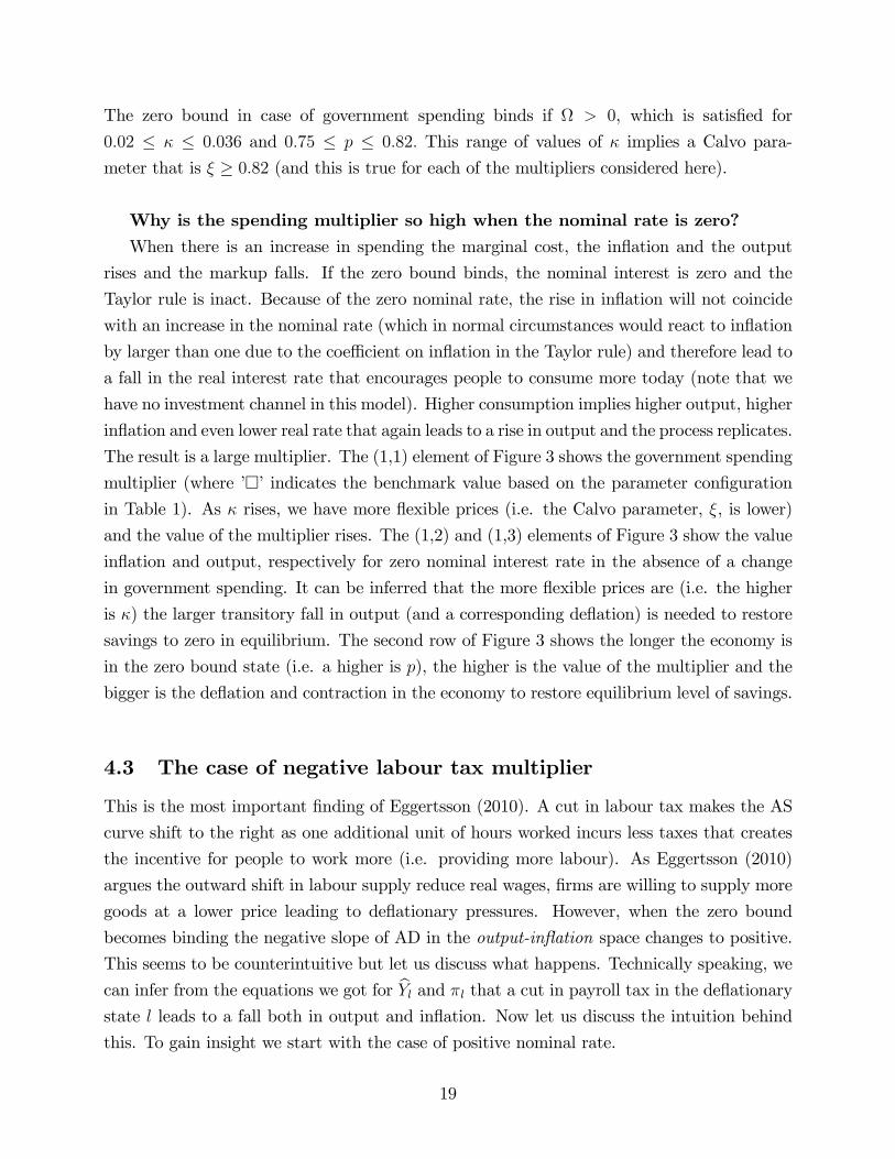
The zero bound in case of government spending binds if > 0, which is satis�ed for

0:02 � � � 0:036 and 0:75 � p � 0:82: This range of values of � implies a Calvo para-

meter that is � � 0:82 (and this is true for each of the multipliers considered here).

Why is the spending multiplier so high when the nominal rate is zero?When there is an increase in spending the marginal cost, the in�ation and the output

rises and the markup falls. If the zero bound binds, the nominal interest is zero and the

Taylor rule is inact. Because of the zero nominal rate, the rise in in�ation will not coincide

with an increase in the nominal rate (which in normal circumstances would react to in�ation

by larger than one due to the coe¢ cient on in�ation in the Taylor rule) and therefore lead to

a fall in the real interest rate that encourages people to consume more today (note that we

have no investment channel in this model). Higher consumption implies higher output, higher

in�ation and even lower real rate that again leads to a rise in output and the process replicates.

The result is a large multiplier. The (1,1) element of Figure 3 shows the government spending

multiplier (where ���indicates the benchmark value based on the parameter con�gurationin Table 1). As � rises, we have more �exible prices (i.e. the Calvo parameter, �, is lower)

and the value of the multiplier rises. The (1,2) and (1,3) elements of Figure 3 show the value

in�ation and output, respectively for zero nominal interest rate in the absence of a change

in government spending. It can be inferred that the more �exible prices are (i.e. the higher

is �) the larger transitory fall in output (and a corresponding de�ation) is needed to restore

savings to zero in equilibrium. The second row of Figure 3 shows the longer the economy is

in the zero bound state (i.e. a higher is p), the higher is the value of the multiplier and the

bigger is the de�ation and contraction in the economy to restore equilibrium level of savings.

4.3 The case of negative labour tax multiplier

This is the most important �nding of Eggertsson (2010). A cut in labour tax makes the AS

curve shift to the right as one additional unit of hours worked incurs less taxes that creates

the incentive for people to work more (i.e. providing more labour). As Eggertsson (2010)

argues the outward shift in labour supply reduce real wages, �rms are willing to supply more

goods at a lower price leading to de�ationary pressures. However, when the zero bound

becomes binding the negative slope of AD in the output-in�ation space changes to positive.

This seems to be counterintuitive but let us discuss what happens. Technically speaking, we

can infer from the equations we got for bYl and �l that a cut in payroll tax in the de�ationarystate l leads to a fall both in output and in�ation. Now let us discuss the intuition behind

this. To gain insight we start with the case of positive nominal rate.

19

Figure 3: Sensitivity analysis of government spending multipliers in case of zero nominalinterest rate for parameters � and p:

0.02 0.03 0.041.05

1.1

1.15

1.2

1.25

κ

Gov. spending mult.

dY/dG

0.02 0.03 0.04­30

­25

­20

­15

­10

­5

κAP

R

Inflation

π l

0.02 0.03 0.04­16

­14

­12

­10

­8

­6

κ

% d

evia

tion 

from

 st.s

t.

Output

Yl

0.75 0.8 0.851

1.05

1.1

1.15

1.2

p

Gov. spending mult.

dY/dG

0.75 0.8 0.85­25

­20

­15

­10

­5

p

APR

Inflation

π l

0.75 0.8 0.85­14

­12

­10

­8

­6

­4

p

% d

evia

tion 

from

 st.s

t.

Output

Yl

In the absence of zero nominal interest, the reaction of the central bank to de�ation is a

cut in the nominal interest rate by more than one-to-one with in�ation (this is the famous

�� > 1 requirement in the Taylor rule). If the in�ation speeds up then the answer of the

central bank is an increase in the nominal rate by more than one-to-one with in�ation. Thus,

in case of de�ationary pressures the real interest rate will decline as the central bank will cut

nominal interest rate by more than one in proportion to in�ation.

However, this is no longer true when the zero bound binds and the central bank cannot

cut interest rates to mitigate de�ationary shock. As the zero bound becomes binding the

de�ationary spiral will induce a rise in the real rate which, as a consequence, lead to a fall

in output. That is, the downward-sloping AD curve in the in�ation-output space becomes

upward sloping when the zero bound becomes binding. Accordingly, we can say that a

simple New Keynesian model with Calvo pricing implies that labour tax is contractionary in

an environment of zero policy rate (Eggertsson, 2010).

The payroll tax multiplier for separable preferences and under the assumption that the

20

nominal rate is zero is given by coe¢ cient on b�Wl in equation (13):

dbYl�db�Wl =

(1� g)p�(1� �W ) ;

where > 0 is needed for the zero bound to bind. This is satis�ed for the the same � and p

parameter intervals as in case of government spending.

The payroll tax multiplier is depicted on the element (1,1) of Figure 4 for a range of �. The

elements (1,2) and (1,3) of Figure 4 show the de�ation and contraction in output associated

with the zero bound state is increasing in � in the absence of a change in payroll tax. As

we can see on (2,1) element of Figure 4 the longer the economy is in the zero bound state

(i.e. the higher is p) the smaller is the payroll tax multiplier (i.e. it is more negative) and

the bigger is the associated de�ation and contraction in output needed to decrease savings

to zero level, shown, respectively on (2,2) and (2,3) elements of Figure 4.

Figure 4: Sensitivity of labour tax multiplier for the case of zero nominal interest rate forparameters � and p:

0.02 0.03 0.04­2

­1.5

­1

­0.5

0

κ

 Labour tax cut

dY/­d τW

0.02 0.03 0.04­30

­25

­20

­15

­10

­5

κ

APR

Inflation

π l

0.02 0.03 0.04­20

­18

­16

­14

­12

­10

­8

κ

% d

evia

tion 

from

 st.s

t.Output

Yl

0.75 0.8 0.85­1.6

­1.4

­1.2

­1

­0.8

­0.6

­0.4

­0.2

p

Labour tax cut

dY/­d τW

0.75 0.8 0.85­25

­20

­15

­10

­5

p

APR

Inflation

π l

0.75 0.8 0.85­18

­16

­14

­12

­10

­8

­6

p

% d

evia

tion 

from

 st.s

t.

Output

Yl

The working of sales tax cut and capital tax cut multiplier for zero nominal rate is rather

similar to the government spending and the corresponding discussion and graphs are omitted

here.

21

5 Summary of temporary �scal multipliers

As we discussed previously multipliers can be higher or equal to one if we have non-separable

preferences or if the economy is in the zero lower bound state. The summary of the analytic

multipliers obtained under the assumption of positive or zero interest rates can be seen in

Table 2. With separable preferences the government spending multiplier is very close to one

although never bigger than one. With certain parametrisation� e.g., choosing coe¢ cient on

output gap, �Y , zero in the Taylor rule in equation (6)� we can obtain a multiplier that is

slightly larger than one for the non-separable case.

We can see that the multiplier for non-separable preferences is nearly as large as the

multiplier in the separable case with zero interest rate (R = 0). Eggertsson (2010) report

high numbers (with values above two) for government spending and sales tax cut multiplier

for zero interest rate (for separable preferences). But, now, I argue, that the government

spending and sales tax multiplier are lower for separable preferences when the zero bound

binds (the spending multiplier, 1 :10 , is above one while the sales sales tax cut multiplier,

0 :54 , is lower than one in the third column of Table 2) than the ones reported by him. When

we use non-separable preferences to model the zero lower bound� as Christiano et al. (2010)

did� then we can see that the multipliers in the last column of Table 2 are well above one

(these are values 3:7 and 1:63 for spending increase and sale tax cut, respectively).

The labour tax multipliers under zero interest rate are negative irrespectively of the

preference speci�cations, which is the most interesting �nding of Eggertsson (2010). In

the previous section we argued in detail why labour tax multipliers are negative when the

nominal interest rate is zero (it is mainly due to the AD curve, which has a negative slope

under positive nominal interest rate, becomes positively-sloped under zero interest rate).

As we can see in the last row capital tax cut is not a good way to stimulate output as

the multipliers are negative irrespectively whether we are in or out of the zero bound state.

We can discuss how sensitive these results to the underlying parameter values. Table 8

in Appendix use a parametrisation that di¤ers from the one in Table 1 only in parameter

choice for �Y� originally set to zero implying no response of monetary policy to changes in

output gap� which is set to the value 0:5=412 as in Taylor (1993). We can observe that this

change� quite counter-intuitively� results in a lower spending multiplier for non-separable

preferences compared to the separable one when interest rate is positive. However, the

sales tax cut multiplier remains to be higher for non-separable preferences after the change

in �Y but the di¤erence in magnitude between the separable and non-separable case fell

considerably.

12We have quarterly data, thus, we have to divide the value of �2 by four.

22

Table 2: Summary of Multipliers� Temporary �scal policy

Multipliers Separable Non-separableR > 0 R = 0 R > 0 R = 0

Gov. spending, dbYtd bGt 0.9675 1.1027 1.052 3.7

Payroll tax, dbYt�db�Wt 0.2318 -0.941 0.1691 -2.38

Sales tax, dbYt�db�St 0.4398 0.5389 0.796 1.63

Capital tax, dbYt�db�At -0.0121 -6.1227 -0.0282 -0.7692

Remarks to Table 2: here we used the parametrisationgiven in Table 1. When R > 0; The multipliers areobtained by using the method of of undeterminedcoe¢ cients. When R = 0 these are given by coe¢ cients onvariables bGt;b�Wt ;b�St and b�At in equation (13).

6 Permanent changes in �scal policy

Suppose now that the change in �scal policy� though slightly unrealitically� is permanent

similar to the experiment by Cogan et al. (2010). Eggertsson (2010) also considered perma-

nent �scal action in his new-Keynesian framework using separable preferences. Now let us

assess the robustness of the results of Eggertsson (2010) when we employ the non-separable

preferences setting of Christiano et al. (2010) to obtain multipliers of a permanent change.

When modelling a permanent change in policy we assume that the variables take on their

long-run(permanent) values immediately with no implementation lag. Similarly to Eggerts-

son (2010) we can distinguish between three cases (let us assume that at time t = T the

zero bound ceases to bind): 1) in the long run, that is, in t � T when the zero bound doesnot bind; 2) in the short run, t < T , when the zero bound doesn�t bind and a Taylor rule is

in action (in that case the algebraic condition [see below] for a binding zero lower bound is

not satis�ed) and 3) short run, t < T , when the zero bound binds and nominal interest is zero.

In case 1 when all variables take their long-run values (output, in�ation and �scal ones

are denoted subscript L) at the time of announcement and bYL and �L can be expressed,

23

respectively, by the following closed form equations13:

bYL = ��(1� g)(�� � 1)(1� )�(1� �W ) b�WL � �(1� g)(�� � 1)(1� )�(1 + �S)

b�SL+�(�� � 1)(1� )

�bGL + %(1� �)(1� )(1� g)

�(1� �A) b�AL ;with � � b�(�� � 1) + (1� g)(1� �)(1� )�Y and

�L =�b%

[��Y + (�� � 1)] (1� �A)b�AL (15)

� ���Y[��Y + (�� � 1)�b] (1� �)

�1

1� gbGL � 1

1� �W b�WL � 1

1 + �Sb�SL�

with � � (1� g)(1� )(1� �); a � 1��W1+�S

and b � 1� + a .

In case 2 when output and in�ation take their short run values� while �scal variables

jump to their long-run levels at the time of announcement� we have a closed form solution

with a positive nominal interest rate14 that is governed by the Taylor-rule in equation (6).

Hence, the nominal interest rate in the short is positive (Rl > 0) and the closed form

expressions for bYl and �l can be written, respectively, as:bYl = � B(1� g)

A(1� �A)

�b�AL + BA

�(1� g)(p� ��)�(1 + �S)(1� p�)

�b�SL+B(1� g)(p� ��)�A(1� �W )(1� p�)b�WL + B

A

�(1� g)(1� p)(1� p�) + (1� g)p�(1� p)

1� p�

��L

+B(1� p)c

AbYL � B(p� ��)�A(1� p�)

bGLwith A

B �fc(1�p)+(1�g)�Y g(1�g)(1� )(1�p�)�(1�g)(p+��)�b

(1�g)(1� )(1�p�) and

�l =�%

�(1� �A)b�AL + �(1� p)��L +

�(1� p)c�(1� g)

bYL���(1� )(1� �)

�(1� �)

�1

1� gbGL � 1

1� �W b�WL � 1

1 + �Sb�SL�

13We calculate tax cuts or spending increase separately. That is, when there is a labour tax cut, dbYl=db�Wl ,there is no change in government spending, bGl = 0, and in other taxes (b�Sl = b�Al = 0) as well as theirsteady-state is zero, i.e. �S = �A = 0; g = 0 but �W > 0. Otherwise, we should specify a budget rulethat governs the relationship between the timing of spending and taxes. E.g. we can imagine, though quiteunrealistically, a balanced budget rule which says that current taxes should �nance current spending.14The algebraic condition for a binding zero lower bound fails to be satis�ed in this case.

24

with � � �(1� )(1��)+�(���p); � � c(1�p)+(1�g)�Y ; and c � �[(1��) (1�a)�1].

In case 3 output and in�ation are, again, determined on both short run (bYl and �l) andlong-run (bYL and �L) while �scal variables take their permanent (or long-run) level. Thealgebraic condition for the zero lower bound is satis�ed (see below). Hence, nominal interest

rate is zero, Rl = 0. Consequently, bYl and �l can be written, respectively, as:bYl = D(1� g)�

C rl +D(1� p)c

CbYL + DC

�(1� g)p�(1� p) + (1� g)(1� p)(1� �p)

1� �p

��L

+DC

�1� g1� �A

�%b�AL + D�(1� g)p

C(1� �W )(1� �p)b�WL+DC

�(1� g)p�

(1� �p)(1 + �S)

�b�SL � D(1� g)p�C(1� �p)bGL;

with CD �

c(1�p)(1�g)(1� )(1��p)�(1�g)p�b(1�g)(1� )(1��p) and

�l =�c(1� p)2(1� )

��L �

�c(1� )(1� p)�

�1

1� gbGS � 1

1� �W b�WS � 1

1 + �Sb�SS�

+�b%

�(1� �A)b�AL + �(1� p)b��L +

�(1� p)cb�(1� g)

bYL + �b��rl

with � � c(1 � )(1 � �p)(1 � p) � �pb. The algebraic requirement for the zero bound tobind is C > 0 which is satis�ed for 0:028 � � � 0:0365 (or, equivalently, 0:83 � � � 0:85).That is the Calvo parameter, �, should be su¢ ciently large.

In case of permanent �scal policy� in contrast to the temporary one� we have to take into

consideration the long-run disin�ationary e¤ect (the e¤ect of lower long-run in�ation expec-

tations) of the increase (decrease) in spending (taxes). This e¤ect is present due to the central

bank�s commitment of in�ation stabilisation (in the form of the Taylor rule). Therefore, the

long-run multipliers (in column 4 of Table 3) have to be corrected by de�ationary pressures

(in column 5 of Table 3) i.e. long multipliers result as the sum of column four and two times

column �ve for each row. The disin�ationary e¤ect is quite small for government spending

and capital tax cut (they might as well be disregarded). If we suppose that the central bank

focuses exclusively on in�ation stabilisation� which is a reasonable assumption� then disin-

�ationary e¤ect of the �scal policies disappears (that is, the coe¢ cients on some of the �scal

variables in equation (15) are zero as now we have �Y = 0). In column 5 we can see the

net multipliers after taking account of the disin�ationary expectations. We have the highest

values for government spending and labour tax cut.

In column 2 of Table 3 we can see that the sales and labour tax multipliers in the short

25

Table 3: Summary of Multipliers� Permanent �scal policy

Multipliers Short-run Short-run Long-run Long-run Total e¤ect

(dbYL=d bXL)y (d�L=d bXL)y�dbYLd bXL + � d�Ld bXL

�y

R > 0 R = 0 R > 0 R > 0 Col.4+�*Col.5

Gov. spending, dbYtd bGt 0.0194 -1.7752 0.6750 -0.0051 0.6648

Sales tax, dbYt�db�St 0.193 -1.921 0.6442 -0.1814 0.2814

Payroll tax, dbYt�db�Wt 0.2863 -1.9438 1.0387 -0.2647 0.5093

Capital tax, dbYt�db�At -0.0221 -0.2063 0.0000 -0.0192 -0.0384

Remarks to Table 3: the results here are derived using non-separable preferences.Eggertsson (2010, pp. 31) has a similar table where he used separable utility.However, his results and ours are not directly comparable because he useddi¤erent calibration. yIn the last column we can see the total e¤ect of a permanentincrease in spending or tax cut, XL = f bGL;b�SL;b�WL ;b�ALg:run when interest is positive have some non-trivial positives values (smaller than one), while

government spending increase and capital tax cut have negligible e¤ects.

In column 3 of Table 3 we realise that all �scal policy multipliers are large negative

number under permanent �scal. However, this was not the case under temporary policy

when government spending and sales tax cut was positive while labor tax cut and capital tax

cut was negative (see column 3 and 5 in Table 2).

It is useful to discuss why permanent increase in spending in the zero bound state (column

3, R = 0) is contractionary. First, observe that there is no direct e¤ect of spending on the

long run when interest is positive because G terms drop out from the Euler equation (both

Gt and Gt+1 take on their long run value GL). Let us turn to the case in column 3 when

the zero bound binds. In this case expected output and in�ation takes their long-run values,bYL; �L, with probability 1 � p. Previously, we claimed that the only thing that mitigatesthe downturn of the economy is a spending spree in the zero bound state. The AD curve is

positively-sloped in the zero bound as explained in the previous section. The rise in spending

generates a decrease in consumption due to the wealth e¤ect and shifts out the labor supply

curve which causes recession when the AD curve is positively sloped. However, when we are

out of the zero bound state (and the Taylor rule is in action) the net e¤ect of spending hinges

on the de�ationary term ( d�Ld bGL ) that is due to the commitment of monetary policy (see results

in column 2).

26

7 Adding capital to the New Keynesian model

In this section we assume that both households and �rms can also use some of their resources

to invest into capital. The government is still supposed to make purchases that are �nanced

by lump-sum taxes. Moreover, we also include capital adjustment costs into the model to

be able to match the observed slugishness of real variables to shocks. Accordingly, both

household�s and intermediate goods �rms�problems change after the inclusion of capital.

Again, following the notations of Christiano et al. (2010), we start with the household�s

optimisation problem.

7.1 The household�s problem

The household maximises the following non-separable utility in consumption (Ct) and leisure

(1�Nt):

U = E0

1Xt=0

�t

"[C t (1�Nt)1� ]

1�� � 11� �

#(16)

with respect to its budget constraint

(1 +Rt)Bt +

Z 1

0

profitt(i)di+

Z 1

0

PtWtNt(i)di+

Z 1

0

PtRktKt(i)di

= Tt +Bt+1 + PtCt + PtIt (17)

where Rkt denotes the real rental rate of capital which serves as an income for the household

and It denotes investment as a further way of spending.

There is an equation that describes the accumulation of capital. According to this equa-

tion, investment is the change in capital stock from time t to time t+ 1:

Kt+1 = It + (1� �)Kt ��I2

�ItKt

� ��2Kt (18)

where the last term on the RHS is the capital adjustment cost that is now speci�ed as

quadratic. The parameter �I > 0 governs the magnitude of adjustment costs to capital

accumulation. That is, the household�s problem is to maximise its utility in equation (16)

subject to its budget constraint in equation (17) and the capital accumulation equation (18).

7.2 The �nal and intermediary goods�producers problem

The �nal good producers�problem remains the same while the intermediary �rms�problem

can be written as follows. Intermediaries set their prices in Calvo manner as it is in model

27

in section one. The ith intermediary maximises its discounted pro�t:

Et

1XT=0

�t+Tvt+T�Pt+T (i)Yt+T (i)� (1� �)

�Pt+TWt+TNt+T (i) + Pt+TR

kt+TKt+T (i)

��; (19)

where Nt(i) and Kt(i) denotes the value of labour and capital used by ith intermediary,

respectively. As we can see from the above formulation the costs are made up of two parts:

labour and capital rental costs, respectively. The output of the ith is produced by:

Yt(i) = [Kt(i)]� [Nt(i)]

1�� : (20)

Similarly to the model in the �rst section we assume that the monopolist markup in the

steady-state is eliminated by a �scal subsidy, that is, � = 1=�: Also note that vt+T corresponds

to the Lagrange multiplier on the budget constraint in the household�s optimisation problem.

Accordingly, the ith intermediary maximises the expression in equation 19 with respect to

the production function in equation (20) and the demand function for Yt(i) in equation (1).

The conduct of monetary and �scal policy is not a¤ected by the inclusion of capital into

the baseline model.

7.3 Equilibrium

De�nition 2 A monetary equilibrium is a collection of stochastic processes which contains

endogenously determined quantitites fYt(i); Yt; Nt; Nt(i); Kt; It; Bt+1;MCt;Mt; Ftg, (shadow)prices fPt(i); P �t ; Pt; �t;Wt; Rt; R

kt ; Qt; vt; #t;�tg and an exogenous process fGtg with initial

conditions K0 and G0. The Intratemporal condition in equation (11) and the Euler equation

(12)15 are exactly the same in the model with capital and they are not listed again here. How-

ever, after taking the derivative of the households� problem with respect to It and Kt+1 we

get two additional equilibrium conditions (see equation 21 and 22 below). The aggregate re-

source constraint� which, now, contains investment as well� is satis�ed. Furthermore, there

is market clearing in goods, labor and capital markets.

Firstly, there is a connection between capital and investment that also involves Tobin�s

Q i.e. the consumption value of an additional unit of capital16:

1 = Qt

�1� �I

�ItKt

� ���; (21)

15However, the NKPC should be written in recursive form instead of the loglinear one. And, of course, thereal marginal cost changes after including capital into the model.16This �rst order condition is obtained by taking the derivative of the Lagrangian associated with the

houshold�s problem with respect to It:

28

which formula implies the mean reversion of It=Kt toward its steady-state value, �: In Chris-

tiano et al. (2010) interpretation, the latter equation implies that an increase in investment

by one unit raises Kt+1 by 1��I�ItKt� ��unit i.e., due to capital adjustment cost Kt+1 rises

by less than one unit.

Secondly, there is another equilibrium condition describing the dynamics of Tobin-Q that

can be derived from the household�s problem17:

#t�#t+1

=1

Qt

(Rkt +Qt+1

"(1� �) + �I

2

�It+1Kt+1

� ��2� �I2

�It+1Kt+1

� ��It+1Kt+1

#)(22)

where #t � [C t (1�Nt)1� ]��C �1t (1 � Nt)1� : As there is no money in the model we

measure capital in consumption units as well. One unit of consumption good worth 1=Qtunits of installed capital. In order to understand the intuition behind equation (22) we have

to observe that the LHS equals the real interest rate based on the Euler equation in (12)18.

Thus, the LHS equals real return on one-period bonds. The real return of installed capital

(the RHS of equation 22) is composed of the following terms: the �rst term on the RHS of

equation 22 is the marginal product of capital, the second term is the undepreciated capital

in consumption units, (1 � �)Qt+1 and the third and fourth terms capture the reduction inadjustment costs as the value of installed capital increase from time t to time t + 1: As a

result, equation (22) can be interpreted as a no-arbitrage condition (Christiano et al., 2009).

When we analyse the case of binding zero bound we assume that the monetary authority

holds the interest rate at constant level. In order to be able to analyse the zero lower bound

in Dynare we have to compute the equations in their original form (that is, not in log-linear

form)19. However, the NKPC is a log-linear equilibrium condition. Alternatively, we can

express NKPC in recursive form. For this purpose let us express the ratio of optimal price,

P �t , and the economy-wide price index, Pt, recursively as:

P �tPt=Mt

Ft;

where Mt and Ft are given, recursively, by:

Mt = #tMCt + ��Et���t+1Mt+1

17Note that, in equilibrium, Rkt equals the real marginal product of capital, i.e. R

kt = �Et

�K��1t+1 N

1��t+1

�:

18The Euler is given by: 1 = Et�� #t+1#t

1+Rt+1

Pt+1=Pt

�with corresponding stochastic discount factor, #t:

19When equations are computed into the Dynare in log-linear form they are not allowed to contain con-stants. When zero bound on nominal interest rate binds, nominal interest rate in the Taylor rule is held atconstant level and this is the reason why the log-linear setup in Dynare is not suitable for the analysis of themodel when the nominal interest rate is zero.

29

and

Ft = #t + ��Et����1t+1Ft+1

:

Accordingly, the expression for the real marginal cost changes to:

MCt = &�Rkt��W 1��t ;

with & � ���(1� �)�(1��):The labour and capital demand of intermediate goods �rms are given, respectively, by

Nt = (1� �)MCtWt

Yt

Z 1

0

�Pt(i)

Pt

���di � (1� �)MCt

Wt

Yt�t;

and

Kt = �MCtRkt

Yt

Z 1

0

�Pt(i)

Pt

���di � �MCt

RktYt�t;

where we have Nt �R 10Nt(i)di;Kt �

R 10Kt(i)di and �t �

R 10

�Pt(i)Pt

���di. The price disper-

sion, �t, can be written recursively as:

�t �Z 1

0

�Pt(i)

Pt

���di = (1� �)

�P �tPt

���+ ����t �t�1:

The economy�s resource constraint after including investment, It, modi�es to:

Yt = Ct + It +Gt:

The government spending shock in the economy is the same as speci�ed by equation (4).

7.4 Calibration

The parametrisation of the model with capital can be found in Table 4. After including

capital, the resource constraint will contain investment as well. We calibrate the share of

capital, �, in the production function by using the values of I=Y; � and �. The value of � and

� are standard in economics literature. We know from Uhlig (2010) that G=Y is 0:18; I=Y is

around 0:22 (the latter is slightly lower than the one in Uhlig (2010) who has international

asset position as well) which implies that C=Y is 0:6. The parameter of the convex adjustment

cost of capital, �I , can be found in Christiano et al. (2010)20. The parameter � is calibrated

20It can be interesting to note that if we use the linearised version of the equation that describes thedynamics of Tobin Q � which is not the case here � then the �I parameter is not needed as we do not needto specify the capital adjustment cost function with a certain functional form that contains �I :

30

to 6 so that we can have a steady-state markup of 20% as in Gali et al. (2007). The value

of �Y is set to 0:5=4 which is the one originally proposed by Taylor (1993). Please also note

that now we consider� more realistically� an environment in which price rigidity is lower (in

the models without capital � was quite high (0:85) but here we set it to 2=3 which implies

that �rms set new prices, on average, every three quarters). The remaining parameter values

are the same as in Table 1.

Table 4: Parametrisation of the New Keynesian Model with Capital

Parameters Separable & capital Non-separable & capital� 2 2' 0.2 na� 0.99 0.99 na 0.29�G 0.8 0.8� 0.025 0.025� 6 6�� 1.5 1.5�Y 0.5/4 0.5/4�R 0 0� 2/3 2/3

G=Y (� g) 0.18 0.18I=Y 0.22 0.22�I 17 17�"G 0.01 0.01

Implied ParametersC=Y 0.6 0.6� 0.17 0.17N na 1/3

31

7.5 Experiments

As we already said in the Introduction (in Section 1) the Bernstein and Romer (BR) (2009)

numbers are based on a permanent �scal stimulus. In the following we restrict the analy-

sis to government spending multiplier only and study� more realistically� the e¤ects of a

temporary, anticipated increase in spending to test the robustness of the numbers of BR

(2009). However, we know that the results are not comparable because BR (2009) assumed

a permanent stimulus in contrast to our temporary one which we think is more realistic. As

we have a forward looking model we have to specify explicitly the assumptions about �rms�

and households�expectations. Here the main assumption is that people expect a temporary

increase in spending that is initially �nanced by issuing debt. Later, the debt is reduced

by levying lump-sum taxes that do lower the after tax income earnings and thereby wealth

(Cogan et al., 2009). In the following we consider three types of multipliers (an impact and

two types of long-run multiplier) under the assumption of �xing the nominal interest rate at

a constant level for one and two years in line with recent empirical evidence on US21.

7.5.1 When nominal interest rate is positive

In Table 5 we can see short and long run multipliers from the model with capital. The

impact multipliers are calculated similarly to the ones in section 2 and 3. The idea of

long-run multiplier is borrowed from Campolmi et al. (2009). It is calculated as the sum of

discounted output changes divided at each time t by the sum of discounted spending changes.

The impact multipliers of spending in the model with capital are generally lower than the

corresponding ones in the model without capital because in the former one an increase in

spending leads to a rise in real interest rate that crowds out private investment (see �ndings

in Table 2 and Table 5). As we can also observe that the impact multiplier is a bit lower

for separable preferences that is in line with our �ndings of section 2. However, the long-run

multipliers, which are generally lower than the impact ones, tell that the distinction coming

from the assumption on preferences disappear on the long run if we assume that there is no

response to changes in output gap in the Taylor rule (i.e. these values are roughly the same;

see numbers with an asterisk Table 5).

21At the time of the introduction of the American Recovery and Reinvestment Package in 2009Q1 it wasnot known for how many quarters the Federal Funds Rate will stay around the zero level. Accordingly, weconsider two experiments: in case 1 we assume that the nominal rate is zero for two years (i.e. the nominalinterest is held �xed on its steady-state level for eight quarters) or case 2 it is held �xed for one year.

32

Table 5: Impact and Long-Run Multipliers of a temporary 1 % spending shock for separableand non-separable preferences

Impact Multiplier(dY=dGjt=1) Long-run MultiplierSeparable 0.7260 0.6884 (0.8726*)Non-separable 0.6966 0.5230 (0.8487*)Remarks to Table 5: the long-run multiplier is de�ned as dividing discountedoutput changes by discounted changes in spending at each time t.*If we assume �Y = 0 in the Taylor-rule then the long-run multipliersare roughly the same.

7.5.2 When nominal interest rate is held constant22

Table 6 shows the response of real GDP to a transitory, anticipated23 increase in government

purchases of 1 per cent of steady-state GDP assuming that the nominal interest rate is held

constant for a duration of two years starting in the �rst quarter of 200924. The latter meansthat the Fed can start to increase interest rate in 2012Q1 at earliest (technically, it means

that the Taylor rule will be put back into practice in 2012Q1). The �rst and second row shows

the �ndings of BR (2009) and this paper, respectively. As we can see the impact multiplier of

the BR (2009) are generally in line with the �nding of ours. However, the latter is not true for

longer horizons. As we can see our multipliers are generally around one at one, two or even at

three years horizon. However, the BR (2009) numbers are much larger than the ones of ours.

Here we can con�rm the �ndings of Cogan et al. (2009) who �nd using a more elaborate (i.e.

containing more frictions) version of the type of model used here that the spending multiplier

should decline with the horizon. However, in contrast to Cogan et al. (2009) who �nd that

multipliers decline sharply with the horizon (with values below 0:5), we show here that the

multipliers can remain over 0:5 (but still below one) even for longer horizons. The di¤erence

between results of Cogan et al. (2009) and ours comes from the fact that while they assumed

permanent stimulus we used a transitory one here. We have seen in the previous section�

using models without capital� that a permanent increase in spending results in middle-sized

multipliers with non-separable preferences (the only exception is labour cut which is around

one). Of course, Eggertsson (2010), who uses separable utility report lower multipliers than

22Here we assume in line with the most elaborate model of Christiano et al. (2009) that the nominal rateis held constant at the natural rate of interest.23Here we assumed that people anticipate the recovery package by two quarters before it is taken into

action. However, for example Uhlig (2009) assumed four quarters.24In a simple New-Keynesian model with capital Christiano et al. (2010) shows that we can endogenously

determine� depending on the properties of the discount factor shock� the date t1 at which zero boundbecomes binding and another date, t2, t2 > t1 at which the zero bound ceases to bind.

33

ours in case of a permanent stimulus.

Figure 5 show a type of long run multiplier calculated similarly to Uhlig (2010). This

multiplier is de�ned as the discounted sum of output changes until each horizon is divided

by the sum of discounted spending changes until the same horizon (Uhlig, 2010). Even on

very long horizons (e.g. after one hundred periods), the multiplier is still around one.

Table 6: Spending multiplier calculated by assuming that the nominal rate is held constantfor two-year duration from 2009Q1 on

Percentage increase in real GDP2009Q1 2009Q4 2010Q4 2011Q4 2012Q4 Long run

BR (2009) 1.05 1.44 1.57 1.57 1.55 naOur �ndings 1.06 0.96 0.93 0.79 0.59 0.85Remarks to Table 6: BR (2009)= Bernstein-Romer (2009) paper. We usednon-separable preferences to perform the calculations in Table 6 and 7.

We re-did our calculations assuming that nominal rate is held constant for a duration

of one year. The results can be observed in Table 7 and Figure 6. As we can see in thesecond row of Table 7, the multipliers are generally lower if nominal interest rate is �xed at

a constant number for a shorter period of time (here it is one instead of two years). Now,

the impact multiplier does not coincide with the one in BR (2009). Also, the longer horizon

�ndings of ours depart even further from the results of BR (2009) while at the same time

approach more the ones of Cogan et al. (2009). However, it has to be pointed out that

our results concerning multipliers of a temporary measure on a time horizon longer than

one year are higher than the ones reported by Cogan et al. (2009) who assumed permanent

stimulus exercise. This �nding is favored by the results obtained from models without capital

in previous sections. Figure 6 shows that the long run multiplier is clearly less than one when

the nominal rate is �xed at constant level for one year.

Table 7: Spending multiplier calculated by assuming that the nominal rate is held constantfor one-year duration from 2009Q1 on

Percentage increase in real GDP2009Q1 2009Q4 2010Q4 2011Q4 2012Q4 Long run

BR (2009) 1.05 1.44 1.57 1.57 1.55 naOur �ndings 0.94 0.78 0.71 0.59 0.55 0.68

34

Figure 5: Uhlig (2010)-type long-run spending multiplier calculated by assuming that thenominal rate is held constant for two-year duration from 2009Q1 on

0 10 20 30 40 50 60 70 80 90 1000.65

0.7

0.75

0.8

0.85

0.9

0.95

1

1.05

1.1

1.15

time

dY/dG

7.6 Further extensions and shortcomings of these types models

The models considered thus far assume that the government de�cit is �nanced through lump-

sum taxes. However, in a recent paper, Uhlig (2010) considers a simple RBC model with

capital, distortionary taxation (that is, labour, capital and sales tax) and a budget rule. In the

budget rule of Uhlig (2010) a certain part of the de�cit plus a random amount is �nanced by

current labour taxes. In the latter case the value of the multiplier is in�uenced meaningfully

by a parameter called budget balance speed de�ning the share of the de�cit �nanced through

labour taxes. If the budget balance speed is su¢ ciently low then the positive e¤ect of a

government spending on output will last longer. However, the most important �nding of

Uhlig (2010) is that the long run multiplier associated with a spending shock is always

negative even if its impact on GDP is positive in the �rst couple of years. Future research

may test the robustness of the �ndings of Uhlig (2010) in a reacher structure including

frictions25 that are popular now in leading New Keynesian models such as the Smets and

Wouters (2007) model.

Hall (2010) points out that the biggest shortcoming of the new-Keynesian models is the

countercyclical markup which is procyclical empirically. Of course, we also emphasized that

25Such frictions include but not restricted to sticky prices and wages, variable capital utilisation, investmentadjustment costs, habit formation and non-Ricardian (i.e. credit constrained) households.

35

Figure 6: Uhlig (2010)-type long-run spending multiplier calculated by assuming that thenominal rate is held constant for one-year duration from 2009Q1 on

0 10 20 30 40 50 60 70 80 90 100

0.65

0.7

0.75

0.8

0.85

0.9

0.95

1

time

dY/dG

the endogenous fall in the mark-up after an increase in spending is a key element of these

type of models. As prices are sticky the the price over marginal cost� which is the de�nition

of the mark-up� falls after an increase in aggregate demand due to an increase in spending.

The estimation of the parameters of the models used here is, of course, also a matter

of future research. For example, Denes and Eggertsson (2009) who estimated the model of

Eggertsson (2010) with Bayesian methods. In particular, Denes and Eggertsson (2009) cali-

brated their model parameters to data prevailing under the Great Depression by maximising

the posterior distribution of his model to match a 30 percent decline in output and a 10 per-

cent de�ation at the �rst quarter of 1933 when the zero lower bound became to be binding

on the nominal interest rate.

36

8 Conclusion

Even if the models presented here are too simple (i.e. they contain only few frictions) for

providing su¢ cient background for policy decisions, still we can obtain a fair picture on the

outcome of possible �scal policy measures. Initially, in a model without capital, we consider

the e¤ects of three di¤erent �scal policy measures that can be used for stimulating the

economy: a temporary and unexpected rise in non-productive government spending, a cut in

sales tax, a cut in payroll tax or a cut in capital tax. Each of them are considered separately

(that is, when government spending increases there is no change in sales or payroll taxes) and

�nanced by lump-sum taxes. Thus, Ricardian equivalence holds. The paper used separable

and non-separable preferences in consumption and leisure as well. Most of VAR evidence

point out that increased government spending lead to a rise in consumption. To model this

stylised fact, we use non-separable preferences in consumption and leisure which imply low

negative Hicksian wealth e¤ect emerging after a rise in government spending in contrast

to separable preferences where negative wealth e¤ect on consumption is high. However, in

the same model with capital we show that the long-run multiplier we borrowed here from

Campolmi et al. (2010) to calculate the long-run e¤ects of a government spending shock

produces roughly the same result for both types of preference speci�cations (these results

depends largely on the underlying parametrisation� e.g., we found, surprisingly, that by

having output targeting in the Taylor rule results in a lower impact and long-run multipliers

for non-separable preferences compared to the separable ones whereas the opposite is true

when we consider in�ation targeting only).

During the recent �nancial crises the nominal interest rate in the U.S. was almost zero,

that is the zero lower bound on nominal interest rate was binding. Based on this stylised fact

we consider the above multipliers in a model with separable preferences when the zero bound

binds and found that the multipliers are smaller than the ones reported by Eggertsson (2010)

and are more close in magnitude to values that we obtain using non-separable preferences

with positive nominal interest rate (the only exception is the labour tax cut which is negative

under zero nominal rate irrespectively of preference speci�cations). However, we found, in line

with Christiano et al. (2010), that a temporary spending stimulus can be turn out to be very

high when holding the nominal interest rate at zero level and assuming non-separable utility.

Moreover, we employed Christiano et al. (2010) non-separable framework to calculate tax

cut multipliers and found that the sales tax cut multiplier is well above one for non-separable

preferences when interest is zero. We show that the most important �nding of Eggertsson

(2010) which says that labour tax cut multiplier is negativ under the separable case for zero

nominal interest, remains true for non-separable utility as well.

37

Some in�uential papers like Cogan et al. (2009) considered permanent stimulus. So

we did and found that it is the government spending and labour tax cut multipliers which

take the highest values under non-separable preferences in case of a permanent stimulus in

contrast to Eggertsson (2010) who found lower values than ours under separable preferences

for the same type of permanent stimulus. Our results show that multipliers of permanent

action must be lower than the same of a transitory one.

Finally, we augmented our model with capital and used three types of multipliers (impact,

long run and Uhlig (2010) type) to compare our �ndings to the ones of Bernstein and Romer

(BR) (2009) and draw the following conclusions. Firstly, it is possible to obtain multipliers

around one on impact similar in magnitude to the ones in BR (2009). Secondly, our temporary

multipliers decline with the horizon similarly to the �ndings of Cogan et al. (2009)� who

calculated multipliers of a permanent stimulus� and in sharp contrast with the results of BR

(2009). Futhermore, the reason why multipliers in Cogan et al. (2010) are lower than ours

is that they consider a permanent stimulus opposed to the temporary ones of ours.

38

9 Appendix

We explained that spending multipliers in the non-separable case are generally higher than

in the separable one (or they are roughly the same), which is true only when the coe¢ cient

on output gap, �Y , in the Taylor rule is chosen to be zero for both positive and zero nominal

interest rates. However, when �Y is chosen to be positive this is not the case any more (see

Table 8) under positive interest rates. Note that the latter �nding is not necessarily true for

sales and labour tax cut multipliers as can be seen in the second and fourth column.

Table 8: Summary of Multipliers� Temporary �scal policy

Multipliers Separable Non-separableR > 0 R = 0 R > 0 R = 0

Gov. spending, dbYtd bGt 0.8382* 1.1027 0.8133* 3.7

Payroll tax, dbYt�db�Wt 0.1931* -0.941 0.1982* -2.38

Sales tax, dbYt�db�St 0.3662* 0.5389 0.5837* 1.63

Capital tax, dbYt�db�At -0.0102* -6.1227 -0.0196* -0.7692

Remarks to Table 8: calibration for these result is thesame as in Table 1 with the only exceptionhere �Y = 0:5=4 as in Taylor (1993) instead of zero. Onlythe multipliers under positive interest rate are a¤ected bythis change (these numbers are denoted with an asterisk).

39

References

[1] Baxter, Marianne and Robert King (1993), "Fiscal Policy in General Equilibrium,�.

AER. Vol. 83, No. 3. 315-334.

[2] Bernstein, Jared and Christina Romer (2009), "The Job Impact of the Amrican Recovery

and Reinvestment Plan, �, memo, The White House.

[3] Bils, Mark and Peter J. Klenow (2004), "Some Evidence on the Importance of Sticky

Prices," Journal of Political Economy. October. 112, 947-985.

[4] Blanchard, Olivier and Roberto Perotti (2002), "An Empirical Characterization of the

Dynamic E¤ects of Changes in Government Spending and Taxes on Output," The Quar-

terly Journal of Economics, Vol. 117, No. 4. pp. 1329-1368.

[5] Calvo, Guillermo (1983), "Staggered Prices in a Utility-Maximizing Framework," Jour-

nal of Monetary Economics 12, 383-398.

[6] Campolmi, Alessia, Ester Faia and Roland Winkler (2010), "Fiscal Calculus in a New

Keynesian Model with Matching Frictions," Working Paper. mimeo. March

[7] Cogan John F., Tobias Cwik, John B. Taylor and Volker Wieland (2010), "New Keyne-

sian versus Old Keynesian Government Spending Multipliers," JEDC, 34 (3), 281-295.

[8] Chrisitiano, Lawrence, Martin Eichenbaum and Sergio Rebelo (2010), "When is Gov-

ernment Spending Multiplier Large?" NBER WP. No. 15394.

[9] Eggertsson, Gauti (2010), "What Fiscal Policy is E¤ective at Zero Interest Rates?"

NBER Macroeconomic Annual.

[10] Denes, Matthew and Gauti Eggertsson (2009), "A Bayesian Approach to Estimating

Tax and Spending Multipliers," New York Fed Sta¤ Report no. 403. November

[11] Gali Jordi, J. David López-Salido and Javier Vallés (2007), "Understanding the E¤ects

of Government Spending on Consumption," Journal of the European Economic Associ-

ation. March.

[12] Hall, Rober E. (2010), "By How Much Does GDP Rise If the Government Buys More

Output?,�Brookings Papers on Economic Activity.

[13] Monacelli, Tommaso and Roberto Perotti (2008), "Fiscal Policy, Wealth E¤ects and

Markups," NBER WP. No. 14584. December.

40

[14] Uhlig, Harald (2010), "Some Fiscal Calculus," AER, forthcoming.

[15] Ramey, V. (2011), "Identifying Government Spending Shocks: It�s All in the Timing,"

Quarterly Journal of Economics, February.

[16] Smets, Frank and Rafael Wouters (2007), "Shocks and Frictions in U.S. Business Cycles:

A Bayesian DSGE Approach," American Economic Review 97, 3:506-606.

[17] Taylor, John B. (1993), "Discretion versus policy rules in practice," Carnegie-Rochester

Conference Series on Public Policy 39, 195-214

[18] Woodford, Michael (2010), "Simple Analytics of the Government Expenditure Multi-

plier," NBER WP. No. 15714.

41