Fluid dynamical Lorentz force law andPoynting theorem—derivation andimplications

D F Scofield1 and Pablo Huq2

1Dept. of Physics, Oklahoma State University, Stillwater, OK 74076, USA2College of Earth, Ocean, and Environment, University of Delaware, Newark, DE19716, USA

E-mail: huq@udel.edu

Received 22 May 2014Accepted for publication 29 June 2014Published 21 August 2014

Communicated by A D Gilbert

AbstractFluid dynamical analogs of the electrodynamical Lorentz force law andPoynting theorem are derived and their implications analyzed. The companionpaper by Scofield and Huq 2014 Fluid. Dyn. Res. 46 055513 gives a heuristicintroduction to the present results. The fluid dynamical analogs are con-sequences of a new causal, covariant, geometrodynamical theory of fluids(GTF). Compared to the Navier–Stokes theory, GTF shows the existence ofnew causal channels of stress-energy propagation and dissipation due to theaction of transverse modes of flow. These channels describe energy-dissipa-tion and transport along curved stream tubes common in turbulent flows.

1. Introduction

This paper presents a rigorous derivation of the fluid dynamical Lorentz force law, the fluiddynamical Poynting theorem, and an analysis of their implications for the theory of fluids. Inso doing, this paper describes a solution to the problem of formulating a covariant, causaltheory of time-dependent fluid flow [2]. This theory is called the geometrodynamical theoryof fluid flow (GTF, [3]). From the GTF equations we derive the fluid dynamical Poyntingtheorem for the transfer of stress-energy. This shows the stress-energy transfer occurs viafinite-speed transverse modes. These modes are excited by the fluid dynamical Lorentz force.The modes lead to new channels of stress-energy dissipation absent from the Navier-Stokestheory. The companion paper [1], provides a heuristic introduction to the Lorentz force lawand Poynting theorem using an analogy to electromagnetic theory [4] for expository purposes.Previously, such electrodynamical analogies have been used to better understand time-

| The Japan Society of Fluid Mechanics Fluid Dynamics Research

Fluid Dyn. Res. 46 (2014) 055514 (22pp) doi:10.1088/0169-5983/46/5/055514

0169-5983/14/055514+22$33.00 © 2014 The Japan Society of Fluid Mechanics and IOP Publishing Ltd Printed in the UK 1

dependent flow; in particular in [5–7] and more recently by Kambe [8]. Kambeʼs work is to benoted for its rigor and for its introduction of a gauge theoretic perspective into such analogies[9]. The present work differs from these since it is not based on analogy; as we show, it isbased on the mathematical consequences of the GTF equations [3]. The theory can describetime-dependent, high speed flows for which inertial forces are balanced by Lorentz forcesalong with enhanced stress-energy dissipation without the introduction of eddy viscosity.

The present paper is organized as follows. The background summarizes the physicalbasis of the theory developed in the companion paper and compares it to the isomorphictheory of electromagnetism. We then derive the fluid dynamical Lorentz force and Poyntingtheorems from the fluid dynamical vortex field tensor, the fluid dynamical analog of theelectromagnetic field tensor. The consequences of the Lorentz force and Poynting theoremsare then developed by formulating the whole set of geometrodynamical theory of fluids (GTF)equations. This is followed by an analysis of the inclusion of the newtonian viscous stressesto assess how these stresses compare to the new channels of stress-energy provided by thevortex field. A summary and conclusion section follows. The first appendix gives the defi-nitions of the tensors used in the formal derivations. The second appendix shows the for-mulation presented here can be expressed in a way that the GTF vorticity ω and swirl ζ fieldshave the same units as the vorticity Ω = × u and Lamb Λ Ω= × u vectors have in theNavier-Stokes theory (NST).

2. Background

In the companion paper we show the need to revisit the foundations of fluid mechanics arisesfrom complications due to the Navier-Stokes equations being parabolic partial differentialequations (PDEs) rather than being cm-Lorentz covariant hyperbolic PDEs. Their diffusionequation formulation, with an attendant infinite speed of velocity propagation, implies action-at-a-distance, a formulation that is termed acausal. On the other hand, a finite speed ofpropagation of signals allows causes and effects at any field point to be sequentially orderedby arrival time. An infinite speed of propagations leads causes and effects to be simultaneous.In the companion paper we discuss the fact the Navier-Stokes equations (NSEs, [2]) areacausal. The NSEs embody action-at-a-distance where all causes arrive from infinitely distantplaces simultaneously but they are not non-causal where effects can precede causes. Thisaction-at-a-distance is a characteristic of newtonian physics where the speed of all signalpropagation is infinite. We also point out for time independent flows, because there is nochange, that there is no propagation at any speed. In this case, the Navier-Stokes equationsreduce to elliptic PDEs having laminar flow solutions.

The problems of the non-relativistic NSEs extend to the relativistic formulation of fluiddynamics given by Landau and Lifshitz [2]. Their fluid theory is an example of a covariant,acausal theory holding the speed of light c constant. It is presently the standard theory ofrelativistic fluids. The acausality of this theory [10] has been discussed extensively[11–17, 19]. This analysis concludes, given there was no alternative theory at the time, thatthe Landau and Lifshitz formulation was adequate as long as the fluid could relax sufficientlyfast enough to mask the acausality. This work also shows a finite speed of wave propagationis a necessary (but not sufficient) ingredient of causal theories.

The geometrodynamical theory of fluids (GTF) given in [3] shows it is possible to avoidthese shortcomings by using a theory based on the geometrodynamics of current conservingspacetimes with finite speeds of transverse wave propagation. The GTF introduces Lorentzforces and Poynting theorems for both fluid dynamics and electrodynamics. In the companion

Fluid Dyn. Res. 46 (2014) 055514 D F Scofield and P Huq

2

paper we describe the resulting, causal theory of fluid mechanics (GTF) by relating it to theanalogous theory of electromagnetism (EMT). Each of these theories respect a maximumspeed of wave propagation that depends on the material medium. Both theories are causaltheories and can be expressed in a covariant form where the basic equations of the theory areform invariant under transformations of coordinates. Both are also Lorentz-covariant,meaning the form of the equations are invariant with respect to transformations of thespacetime coordinates even including coordinate systems moving at constant relative speedsto the flow. Both theories involve covariant 4-currents. We describe the calculation of thefluid 4-current in this paper.

Integral to the GTF theory is the existence of a maximum speed of transverse waves,denoted cm and two other phenomenological constitutive parameters that we discuss in thenext section. For a fluid continuum a finite speed of propagation is also required to escape theconundrum of newtonian physics action-at-a-distance and infinite speeds of transverse modepropagation characteristic of the NST. Avoiding this problem is required if one is to con-sistently combine transverse mode propagation (fluid dynamical Lorentz forces) and covariantstress-energy flux balance. Experimental measurements show the maximum speeds of fluiddynamical waves cm is of an order 10−5 times smaller than the maximum speed of propagationof light waves in empty space, the speed of light = × −c 2.9979 10 m s8 1, [20–22]. Becauseof this limitation, the geometry of the spacetime required for fluids acting under a fluid vortexfield must employ the smaller by ×−10 5 speed of propagation. The questions raised by theanalysis of [11–19], then implies relaxation times are no longer relatively short, so analternative theory to the relativistic NST of [2] needs to be formulated (e.g., GTF).

In summary, causality is physically related to the existence of a maximum speed of signalpropagation and mathematically to the use of hyperbolic, second-order wave equations with asingle time-like variable. In a sense, it is remarkable that finite speed of signal propagation,causality, and spacetime geometries are so intimately related. In the following parts of thispaper, by introducing a finite speed of propagation c ,m a covariant, causal theory of fluids isformulated that is expressible in terms of hyperbolic wave equations and covariant stress-energy flux balance, —the GTF theory. This enables the derivation of fluid dynamical Lor-entz forces and energy transport described by Poyntingʼs theorem.

2.1. Vortex Field Equations

Causal theories such as electrodynamics address the foundational problems of the propagationof stress and energy in a continuum. They require a finite speed of propagation. This allowsthe concept of ‘transport’ of causes to effects to be meaningfully defined. In this we caninclude in ‘transport’ a combination of convection and propagation. The vortex fieldequations introduced immediately below are causal equations formingg part of the GTF. Asexplained in the companion paper, these equations allow one to describe the propagation, notacausal diffusion, of the velocity, vorticity, and swirl fields contributing to the stress-energyflux balance in a fluid. In the remainder of this section, we will give a synopsis of the vortexfield equations and the terms used to describe the balance of stress-energy flux in a cm-spacetime. The basic result is the following:

Theorem 1. Vortex Field Equations (VFEs, Scofield-Huq, [3]). Consider a simplyconnected 4D cm-ST manifold and a homogeneous, isotropic fluid having a linear constitutiverelation between its vortex field ζ ωF ( , ) and its excitations H(ζ ω¯ ¯, ), =κλ κλ

μνμνH C F . Then the

conservation of the 4-current J for homogeneous isotropic media implies the

Fluid Dyn. Res. 46 (2014) 055514 D F Scofield and P Huq

3

geometrodynamical theory of fluid (GTF) vortex field equations and an isomorphism withelectromagnetic theory (EMT) as displayed in table 1.

The isomorphism given in table 1 illustrates the profound consequences of the con-servation of currents [3]; the physical currents in EMT and GTF are quite different, yet theyobey isomorphic vortex field equations. Table 1 illustrates the physical theory analogy.However, the correspondence is deeper. Both EMT and GTF are derived from the vortex fieldlemma, a consequence of the conservation of currents (electrical and fluid, respectively). HereρD is the electrical charge density and JD is the electrical current, the electric field vector isdenoted by E and the magnetic field vector by B. Their excitation fields are the vectors D andH. The parameters κλ

μνC in the theorem statement are linear constitutive (material) parametersof the vortex fields—different from the viscosity parameters of the NST. They relate thevortex field strength ζ ωF ( , ) to its ‘excitations’ ζ ω¯ ¯H ( , ) in the same way the field strengthsF E B( , ) and excitations H(D H, ) are related in electrodynamics [23]. (See ref. [4, section6.8–9] for the analogous case where lossy electromagnetic media is also considered.) Theexcitations ζ ω¯ ¯H ( , ) are related to the fields ζ ωF ( , ) in that the excitations are the response ofthe system to field variations. The excitations of the vorticity ω and swirl ζ fields are denotedwith an over-bar ζ ω¯ ¯( , ). The ζ ω¯ ¯( , ) are not ‘fluctuations’ about a mean. Thus these quantitiesare not directly related to the Reynolds decomposition of mean quantities compared to theirperturbations often used in the analysis of turbulent flow. The variation of the density ρallows one to define the quantity δρ ρ ρ= − avg as the fluid density fluctuation about theaverage value, ρavg; it is also not a Reynolds decomposition. The spatial current componentsare given by ρ=J ui i. In the absence of longitudinal fields due to ρavg so ζ δρ· ¯ = = 0,there is still an analog of the electrical displacement field ζ≃ ¯D( ) whose time variation ζ∂ ¯ ∂tproduces a curl of the analog of the vorticity excitation − λ ζ¯ ∂ ¯

∂c tm+κ ω¯ × ¯ = π

η J.4

Transverse waves are predicted by the equations of table 1 given appropriate geometricconstraints as in electrodynamics [1–4]. For instance, transverse vorticity (TV) waves arepredicted by solving these equations for flow along flow guides of constant cross-section andvanishing velocity along the walls of the guide. Transverse swirl (TS) waves have swirlcomponents transverse to the direction of propagation. Transverse vorticity-swirl (TVS)waves are predicted for propagation in unbounded media. These TV, TS and TVS modescorrespond to the TM, TE and TEM modes of electrodynamics, respectively.

The GTF formulation given in table 1 is general so that we can flexibly determine thephysical units and constitutive relations depending on experimental methodology and theo-retical requirements. Using the flexibility of four constitutive parameters, in appendix B, weshow the equations can be simplified using dimensional analysis so only a total of three

Table 1. The isomorphism derived between the vortex field equations of electro-magnetic theory (EMT) and geometrodynamical theory of fluids (GTF).

EMT GTF

· = B 0 (1) κω· = 0∂∂

+ × =c

B

tE

10

(2) ω λκ

ζ∂∂

+ × =c t

10

m

πρ· = D 4 D (3) ζ πηλ

ρ· ¯ =¯ ¯ c4

m

π− ∂∂

+ × =c

D

tH

cJ

1 4D

(4) ζ κλ

ω πηλ

− ∂ ¯∂

+ × ¯¯ ¯ =

¯ ¯c t

J1 4

m

Fluid Dyn. Res. 46 (2014) 055514 D F Scofield and P Huq

4

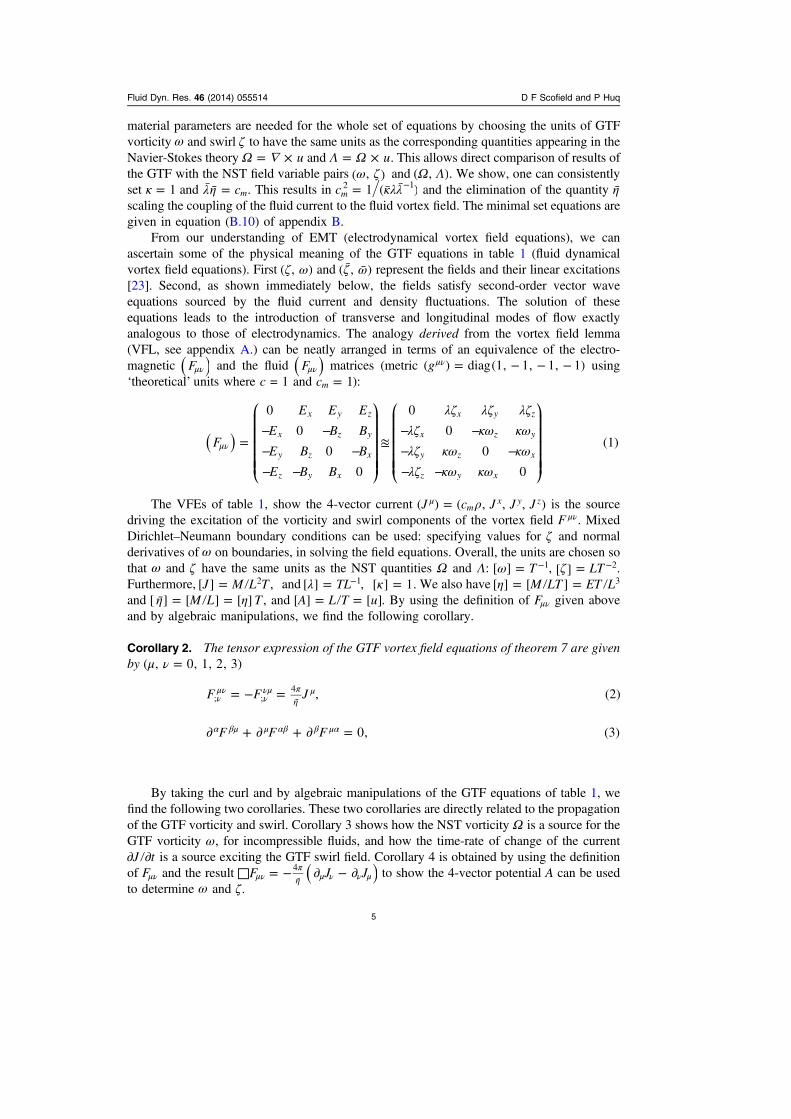
material parameters are needed for the whole set of equations by choosing the units of GTFvorticity ω and swirl ζ to have the same units as the corresponding quantities appearing in theNavier-Stokes theory Ω = × u and Λ Ω= × u. This allows direct comparison of results ofthe GTF with the NST field variable pairs ω ζ( , ) and Ω Λ( , ). We show, one can consistentlyset κ = 1 and λη¯ ¯ = c .m This results in κλλ= ¯ ¯−c 1 ( )m

2 1 and the elimination of the quantity ηscaling the coupling of the fluid current to the fluid vortex field. The minimal set equations aregiven in equation (B.10) of appendix B.

From our understanding of EMT (electrodynamical vortex field equations), we canascertain some of the physical meaning of the GTF equations in table 1 (fluid dynamicalvortex field equations). First ζ ω( , ) and ζ ω¯ ¯( , ) represent the fields and their linear excitations[23]. Second, as shown immediately below, the fields satisfy second-order vector waveequations sourced by the fluid current and density fluctuations. The solution of theseequations leads to the introduction of transverse and longitudinal modes of flow exactlyanalogous to those of electrodynamics. The analogy derived from the vortex field lemma(VFL, see appendix A.) can be neatly arranged in terms of an equivalence of the electro-magnetic μν( )F and the fluid μν( )F matrices (metric = − − −μνg( ) diag(1, 1, 1, 1) using‘theoretical’ units where c = 1 and =c 1m ):

λζ λζ λζλζ κω κωλζ κω κωλζ κω κω

=− −− −− −

≊− −− −− −

μν

⎛

⎝

⎜⎜⎜⎜⎜

⎞

⎠

⎟⎟⎟⎟⎟

⎛

⎝

⎜⎜⎜⎜⎜

⎞

⎠

⎟⎟⎟⎟⎟( )F

E E E

E B B

E B B

E B B

0

0

0

0

0

0

0

0

(1)

x y z

x z y

y z x

z y x

x y z

x z y

y z x

z y x

The VFEs of table 1, show the 4-vector current ρ=μJ c J J J( ) ( , , , )mx y z is the source

driving the excitation of the vorticity and swirl components of the vortex field μνF . MixedDirichlet–Neumann boundary conditions can be used: specifying values for ζ and normalderivatives of ω on boundaries, in solving the field equations. Overall, the units are chosen sothat ω and ζ have the same units as the NST quantities Ω and Λ: ω = −T[ ] 1, ζ = −LT[ ] .2

Furthermore, =J M L T[ ] ,2 and λ κ= =−TL[ ] , [ ] 1.1 We also have η = =M LT ET L[ ] [ ] 3

and η η¯ = =M L T[ ] [ ] [ ] , and = =A L T u[ ] [ ]. By using the definition of μνF given aboveand by algebraic manipulations, we find the following corollary.

Corollary 2. The tensor expression of the GTF vortex field equations of theorem 7 are givenby μ ν =( , 0, 1, 2, 3)

= − =νμν

ννμ π

ημ

¯F F J , (2); ;

4

∂ + ∂ + ∂ =α βμ μ αβ β μαF F F 0, (3)

By taking the curl and by algebraic manipulations of the GTF equations of table 1, wefind the following two corollaries. These two corollaries are directly related to the propagationof the GTF vorticity and swirl. Corollary 3 shows how the NST vorticity Ω is a source for theGTF vorticity ω, for incompressible fluids, and how the time-rate of change of the current∂ ∂J t is a source exciting the GTF swirl field. Corollary 4 is obtained by using the definitionof μνF and the result □ = − ∂ − ∂μν

πη μ ν ν μ¯ ( )F J J4 to show the 4-vector potential A can be used

to determine ω and ζ.

Fluid Dyn. Res. 46 (2014) 055514 D F Scofield and P Huq

5

Corollary 3. The GTF vortex field equations in table 1 imply the following vector waveequations relating the vorticity and swirl fields to the current J and density ρ of the fluid

ω πη

∂∂

− =¯

×⎛⎝⎜

⎞⎠⎟

c tJ

4, (4)

m

2

2 22

ζ πηλ

πλη

ρ∂∂

− = −¯

∂∂

+¯

⎛⎝⎜

⎞⎠⎟

c t c

J

t

c4 4. (5)

m m

m2

2 22

Here κλ κλ= ¯ ¯c .m2

For incompressible fluids of constant density ρΩ× = J , equation (4) shows the NSTvorticity Ω is the source of the GTF vorticity field ω. For constant density, ρ = 0, so the lastterm on the right-hand side of equation (5) vanishes. Thus for incompressible fluids, the timerate of change of the NST vorticity Ω is the source for the GTF swirl field ζ . In this corollarywe notice the maximum speed of propagation cm is determined by the material parameters.

Corollary 4. The swirl ζ and vorticity ω components of the vortex field tensor ζ ωμνF ( , ) canbe obtained in terms of a 4-component gauge potential Φ=μ( )A A( , )i which satisfies avector wave equation μ =( 0, 1, 2, 3)

πη

∂∂

− =¯

μ μ⎛⎝⎜

⎞⎠⎟

c tA J

4. (6)

m

2

2 22

Here the Lorenz gauge condition ∂ =μμA 0 is used. This equation is often written as

□ =μ πη

μ¯

A J ,4 where □ ≡ ∂ − ( ).t2 2

The vector potential does not add new degrees of freedom to the theory. In fact, it allowsthe six linearly independent components of the vortex field of the antisymmetric field tensor

μνF to be computed from four quantities μ( )A simply by differentiation: = ∂ − ∂μν μ ν ν μF A A( ).From equation (6), one can show the vortex field tensor μνF also satisfies a wave equation:□ = ∂ − ∂μν

πη μ ν ν μ¯ ( )F J J .4 Using the definition of ζ ωμνF ( , ) given in equation (1), allows one

to determine the GTF vorticity ω and swirl ζ fields. Solution of equation (6) is thus equivalentto the solution of the vortex field equations of table 1.

These corollaries show how the gauge potential 4-vector μ( )A is sourced by the currentμ( )J and how ζ ω( , ) are obtained from the gauge potential and the current 4-vector. The

isomorphism between electromagnetic field theory [4] and vortex field theory is readilyapparent: the equations for electrodynamical vortex field are of the exact same form as for thefluid dynamical vortex field [3]. Equations (1), providing a formal, linear, invertible (hence 1to 1) mapping between the electromagnetic field tensor and the fluid dynamical vortex fieldtensor, can be seen to be a logical consequence of theorem 1. The analogy (isomorphism)also shows the vortex field equations can be expressed as gauge field equations for the vectorpotential components μA in the same way as in electrodynamics (corollary 4). As shown incorollarys 3 and 4, the theory yields second order wave equations forr which there is an finitelimit to the mode propagation speed cm.

Equations (6) can be solved to determine the transverse modes, for instance, for flows incircular, rectangular or helical pipes. The consequences of being able to compute such modesand categorize the modal structure (topology) of fluid flow are far-reaching. A theory ofhelicity and the topology of inviscid or perfect fluid flows has already been developed basedon an electrodynamic analogy [24–27]. That theory provides a description of helical

Fluid Dyn. Res. 46 (2014) 055514 D F Scofield and P Huq

6

structures for perfect fluids. Using the present theory, GTF, the limitation to perfect fluids isremoved in the context of the NSEs [28, 29]. As a consequence, the work on the topology ofperfect fluid flow, e.g., summarized in references [30] and [31], can be derived from GTFthereby providing an extension of the perfect fluid topology theory to a viscous fluid topologytheory. Such topological quantities are crucial for understanding and predicting propagationand dissipation of stress-energy in flows with transverse mode structures. Thus there nowexists a machinery for computing the vortex field, ζ ω = ∂ − ∂μν μ ν μ νF A A( , ) , just as inelectrodynamics. The vortex field, of course, produces stresses and propagates energy in thefluid. These effects must be included in the stress-energy flux balance.

3. Deriving the fluid dynamical Lorentz force law and Poynting theorems

In this section, we derive the fluid dynamical Lorentz force law and the Poynting theorem. Inappendix A we give the detailed definitions of the tensors involved in our discussion. Ourformulation of the balance of stress-energy flux is based on the one given in [2].

Tensor analytic methods for a 4D cm-spacetime are used in the remainder of this paper.We follow the conventional notation: subscripts indicate covariant components. Superscriptsdenote contravariant components. For a vector of covariant components μJ , the same vectorexpressed in terms of contravariant components is given by =μ μν

νJ g J , where the Einsteinconvention of summing over repeated covariant-contravariant index pairs is used. Greekletter indices vary over {0, 1, 2, 3}. Roman letter ones vary over 1, 2, 3. The metric tensorhas components given by = − − −μνg( ) diag(1, 1, 1, 1) in units where =c 1m , therebydefining the geometry of a Minkowski spacetime. The formulated equations are covariant inform with respect to Lorentz transformations in which cm is held constant. This is called cm-Lorentz covariance. This covariance follows from the isomorphism of the VFEs and Max-wellʼs equations, the latter being c-Lorentz covariant as the maximum speed of transversewaves is the speed of light c. The use of this Minkowski spacetime forms the basis forpreserving causal ordering. A cm-covariant theory can be developed on this basis.3 Thecovariant (cm-ST) derivative is denoted by a semi-colon and a subscript. For the presentdiscussion these covariant derivatives are equivalent to partial derivatives if cartesian coor-dinates are adopted. The 4D spacetime tensor approach is both simpler and more elegantcompared to the (3+1)D formulation used in table 1 and simplifies the derivations of theLorentz force law and Poyntingʼs theorem.

3.1. Fluid dynamical Lorentz force law

In this and the following, section we attend to the rigorous derivations of the Lorentz forceand the Poynting theorem of fluid dynamics. As shown above the fluid dynamical-electro-dynamical analogy is not arbitrary. It is a consequence of the fact that both theories describethe dynamics of conserved currents. We start with the balance of stress-energy flux includinginertial and vortex field contributions

τ τ= − ≡νμν

νμν μν

νF J . (7)e m; ;

This equation also expresses the balance of stress-energy flux in the fluid. Here the quantityon the left-hand side describes the stress-energy flux due to inertia τ μν

e . The quantity τ μνm is the

stress-energy of the fluid vortex field. For completeness, we give the expressions for these

3 Physical quantities (scalars, vectors, or tensors) transform cm-covariantly if they transform according to arepresentation of the Lorentz group having a maximum speed parameter cm. Scalars transform cm-invariantly.

Fluid Dyn. Res. 46 (2014) 055514 D F Scofield and P Huq

7

quantities in appendix A, as derived in [2, p 505]. The derivation of the Lorentz force lawstates the equivalence of this stress to the stress due to the fluid dynamical vortex field. Thederivation of the form of the stress exerted by the vortex field amounts to proving the identityτ ≡ −ν

μν μννF J( ) .m ; Here the symmetric Maxwell stress-energy tensor, also called the energy-

momentum tensor, tensor τ μνm of the vortex field, is expressed by4

πη τ¯ = +μν μααβ

βν μναβ

αβ− g F F g F F4 . (8)m1 1

4

As a consequence of the isomorphism between the vortex field equations for electrodynamicsand for fluid dynamics, the form of the stress-energy tensor in electrodynamics and fluiddynamics have the same form as given in equation (8). The evaluation of the stress-energytensor in terms of the quantities on the right of equation (8) is most easily effected byexpressing all quantities in terms of their corresponding matrix representations. See also [32,pp 65, 87] and note if ζ ω=αβF F ( , ), then ζ ω= −αβF F ( , )). We then apply tensor analysistechniques for evaluating the covariant derivative of τ μν

m to derive the Lorentz force law asfollows. See also [4, section 12.10C]

Theorem 5. Fluid Dynamical Lorentz force law. The force (density) fi acting on the fluidcurrent due to the fluid vortex field is given by ν= =i( 1, 2, 3, 0, 1, 2, 3)

λζ κ ω λζ= = + × = −νν

νν( )f F J J J F J J( ) , . (9)i i i i i

i00

Here ρ=J ui i are the 3-vector components of the fluid current, ζ i and ωi are the vector andpseudo-vector components of the fluid dynamical vortex field tensor μνF .

Proof. We need to evaluate the covariant derivative τ τ∂ ≡νμν

νμν( ) .m m; In this evaluation we

use the identity

∂ = ∂ = ∂

= ∂ = ∂

= ∂

μαν αβ

βνν β

μ βνν

μααβ

βν

νμα

αν

νμα νβ

αβ

β μααβ( )

( ) ( ) ( )( ) ( )

g F F F F F g F

F F F g F

F F

,

,

. (10)

The fact the covariant derivative of the metric tensor vanishes is used. We also use theproduct rule stating the product of an antisymmetric tensor αβF with a symmetric onevanishes, so

∂ + ∂ =αββ μα α μβ( )F F F 0. (11)1

2

There follows the sequence of steps leading to the evaluation of the covariant derivative (Weset η =− 11 on both sides of the equation.)

π τ∂ = ∂ + ∂νμν

νμα

αββν μν

ν αβαβ( ) ( )( ) g F F g F F a4 , (12 )m

14

4 See [4, section 12.10B] for a discussion. The right-hand side of equation (8) can also be written as− +μα μσ

σν μν

αβαβg F F g F F1

4. Sign conventions and metrics are often reversed. In [4] and in [2] and [32] which deal

with the classical theory of electromagnetic and matter fields, the metric is = − − −μνg( ) diag(1, 1, 1, 1) in unitswhere =c 1m . In [33, section 56] which deals with classical theory of spacetime fields, the opposite signature is used.Such an overall sign change does not change the field equations, as seen by the fact the (Euler-Lagrange) equationsderived from opposite signatures lead to the same results at an extremum [32, section 33]. One can show in bothcases the energy-momentum tensor is traceless, τ =ν

ν 0.

Fluid Dyn. Res. 46 (2014) 055514 D F Scofield and P Huq

8

= ∂ + ∂ + ∂μαν αβ

βν μααβ ν

βν μναβ ν

αβ( )g F F g F F g F F b, (12 )12

π= ∂ − + ∂μαν αβ

βν μααβ

β μναβ ν

αβ( )g F F g F J g F F c4 , (12 )12

π= − + ∂ + ∂μααβ

βαβ

μ αβ μαν αβ

βν( ) ( )g F J F F g F F d4 , (12 )12

π= − − ∂ + ∂ + ∂μααβ

βαβ

β μα α βμαβ

β μα( )g F J F F F F F e4 , (12 )12

π= − + ∂ + ∂μνν αβ

β μα α μβ( )F J F F F f4 , (12 )12

π= − μννF J g4 , (12 )

τ∂ = −νμν μν

ν( ) F J h. (12 )m

Equation (12a) expresses the definition of the covariant derivative of τ μν.m Evaluating thecovariant derivative of the last term of that equation gives equation (12b). Equation (12c)applies the tensor form of the vortex field equation πη∂ = ¯ν

νβ β−F J4 1 (With η =− 1.1 ) andcorollary 2. The following equation, equation (12d), involves a rearrangement. Equation (12e)combines the last two terms by applying corollary 2 and the identity, equation (10). To obtainthe next equation, equation (12f), the relation =μα

αββ μν

νg F J F J is used. To get equation(12g) the product rule equation (11), is used. Finally in the last equation, we cancel the factorof πη−4 1. (With η =− 1.1 ) Evaluating the Lorentz force term μν

νF J using equation (1), raisingindices, which changes the sign of the spatial components in the metric chosen, we obtain

λζ λζ λζλζ κω κωλζ κω κωλζ κω κω

λζ λζ λζλζ κω κωλζ κω κωλζ κω κω

=

− − −−

−−

−−−

=

+ ++ −− ++ −

μνν

⎛

⎝

⎜⎜⎜⎜

⎞

⎠

⎟⎟⎟⎟

⎛

⎝

⎜⎜⎜⎜

⎞

⎠

⎟⎟⎟⎟

⎛

⎝

⎜⎜⎜⎜

⎞

⎠

⎟⎟⎟⎟( )F J

JJJJ

J J JJ J JJ J JJ J J

00

00

(13)

1 2 3

1 3 2

2 3 1

3 2 1

0

1

2

3

1 1 2 2 3 3

1 0 3 2 2 3

2 0 3 1 1 3

3 0 2 1 1 2

The theorem statement in equation (9) is obtained from the last three elements of the columnvector defined in this equation and from the first element by using the fact

λζ λζ∑ = −= J Ji i ii

i13 . ■

Examination of the second through fourth elements of the first column of equation (13),shows the right-hand side contains the familiar form of the Lorentz force in the analogy wherethe λζ i are analogous to the components of the electric field Ei and J0 is analogous to thecharge q. The second, third, and fourth lines also involve the components of ω×J . Here, theκωi are analogous to the components of the magnetic induction field Bi. So these lines accountfor the analogy to the u × B of the electromagnetic Lorentz force law. The second relation ofequation (9) is usually omitted in vector analytic derivations. This relation describes effectsanalogous to the ‘resistive’ heating caused by the work of the current against the swirl field. Itvanishes for vortex fields transverse to the current flow, i.e., when ζ· =J 0. All of theLorentz force components can be computed, given a fluid dynamical current and constitutiveparameters, equations (5).

3.2. Fluid dynamical Poynting theorem

The identity τ = −νμν μν

νF J( )m ; , equation (12h), is derived in the proof of the Lorentz force lawabove. A detailed expression for τ μν

m is needed to prove the Poynting theorem. This isprovided by evaluating the various tensor quantities in equation (8). The tensor components

Fluid Dyn. Res. 46 (2014) 055514 D F Scofield and P Huq

9

of τ μν( )m can be arranged in the form [4, section 12.10B], [32–34]

τ τ τ τ

τ τ τ ττ τ τ ττ τ τ τ

ηπ

λ ζ κ ω λζ κω

λζ κωλ ζ ζ κ ω ω

λ ζ κ ω δ

⋮⋯ ⋮ ⋯ ⋯ ⋯

⋮⋮⋮

= ¯

+ ×

×− +

+ +

⎛

⎝

⎜⎜⎜⎜⎜⎜

⎞

⎠

⎟⎟⎟⎟⎟⎟

⎛

⎝

⎜⎜⎜⎜⎜

⎞

⎠

⎟⎟⎟⎟⎟

( )

( )( )

4

col(

col( )(14)

m m m m

m m m m

m m m m

m m m m

j

jj k j k

jk

00 01 02 03

10 11 12 13

20 21 22 23

30 31 32 33

12

2 2 2 2

2 2

12

2 2 2 2

The lower right-hand block τmjk describes the spatial components of the Maxwell stress-energy

tensor. The three spatial components of the top row τmk0 or three spatial elements in the left-

most column τmk0 describe the momentum components of the vortex field stress-energy tensor.

The upper left-hand corner gives the energy τm00. A relationship between these quantities is

determined by differentiating the Maxwell stress-energy tensor. This provides proof of thePoynting theorem that follows.

Theorem 6. (Generalized) Fluid dynamical Poynting theorem. For a simply connected 4Dcm-ST manifold and a homogeneous, isotropic fluid having a linear constitutive relationbetween its vortex field ζ ωF ( , ) and its excitations H(ζ ω¯ ¯, ), satisfying GTF vortex fieldequations displayed in table 1, the Poynting relations hold

λ ζ λ ζ

ηπ

λζ κω λ ζ κ ω

∂∂

+ · = − · = −

=¯

× = +ηπ¯⎜ ⎟

⎛⎝

⎞⎠

( )t

S c J c J

Sc

,

4( ) , . (15)

m mi

i

i m i8

2 2 2 2

Here is the fluid vortex field energy, the Si are the components of the fluid dynamicalPoynting vector, ζ and ω are the vector components of the fluid vortex field μνF , and Ji arethe vector components of the fluid current. The parameters κ and λ are constitutiveparameters for a homogeneous isotropic fluid.

Proof. By using equation (14) in equation (12h) and indicating the differentiations, weobtain

λ ζ κ ω δηπ

λζ κω δ

ηπ

λζ κω δ

ηπ

λ ζ ζ κ ω ω λ ζ κ ω δ δ

λζ

λζ κ ω

∂∂

+¯ ×

¯ ×

− ¯ + + +

=−

− + ×

ν

ηπ

ν

ν

ν

ηπ

ν

¯

¯⎜

⎛

⎝⎜⎜⎜ ⎛

⎝

⎞

⎠

⎟⎟⎟⎟⎛

⎝⎜⎜

⎞

⎠⎟⎟

( )( )

( )

x

J

J J

4( )

4( )

4

( ). (16)

j

j

j k j k jk j

ii

j j

82 2 2 2 0

2 28

2 2 2 2

0

Using =x c t,m0 we then obtain the Poynting theorem of energy density flux from the time-

components:

λ ζ κ ωηλζ κω

πλζ∂

∂+ +

∂ ¯ ×∂

= −ηπ¯( )( ) ( )

c t xJ

4, (17)

m

i

ii

i82 2 2 2

and also a relation for momentum or stress flux (having divided the equation by c )m from thespatial components:

Fluid Dyn. Res. 46 (2014) 055514 D F Scofield and P Huq

10

λζ κω λ ζ κ ω δ ηπ

λ ζ ζ κ ω ω

λζ κ ω

∂∂

× + + − ¯ +

= − + ×

ηπ¯( )( ) ( )

( )x

J J

(2 )4

( ) . (18)

kk jk j k j k

j j

82 2 2 2 2 2

0

This equation provides a generalization of the standard Poynting theorem which is usuallylimited to equation (17). On comparing equations (15) and (17), the Poynting theorem,equation (15), follows.

Examining the structure and physical units used in equations (15) through (18) shows thevortex field modes transport energy and momentum or equivalently stress-energy. Morespecifically, since ω = −T[ ] ,1 ζ = −LT[ ] ,2 λ = −TL[ ] ,1 κ =[ ] 1, η = M L[ ] [ ], η = M LT[ ] [ ],and = − −J ET L L[ ] ,2 2 3 the terms in Poynting theorem, equation (17), are dimensionallyhomogeneous with dimension × ;E

L T

13

energy dissipation rate/unit volume. The dissipationdue to λ ζ− ·c Jm is seen to represent an energy-dissipation rate/unit volume caused bycurrents working against the swirl field. The term λ ζ− ·c Jm gives a velocity dependentcontribution to the energy-momentum dissipation, thereby lending stability to the flowequations in the otherwise unstable high Re limit [35], [36]. This energy-dissipation isanalogous to a ·V I resistive or an I R2 loss in electrodynamics leading to Joule heating. Thevector =S λζ κω×η

π¯

( )c

4m is the analog of the Poynting vector in electromagnetic theory, so

this term describes the net momentum flux · S cm of the mode system. Let us define anenergy-momentum density 4-vector = S S c S c S c( , , ).x

my

mz

m Here we include cm in themetric. Therefore, the fluid dynamical Poynting theorem given in equation (17) can beinterpreted physically as stating the sum of the rate of change of the energy-momentumdensity ∂μ

μS of the transverse mode excitations is limited to the rate λζ Ji i at which the flowcan generate heat, λζ∂ = −μ

μS Ji i. The transport of stress-energy stated in the Poynting the-orem, equation (17), describes new, propagating, channels of energy transport absent inthe NST.

4. Implications of the Lorentz force law and Poynting theorem

4.1. Field equations reflecting new channels of stress-energy transport

The Lorentz force law and Poynting theorem describe the physical effects incorporated intothe GTF, a cm-Lorentz covariant theory of fluid flow. This theory comprises the the equationsexpressing the conservation of the sum of the stress-energy of the inertia τ μν

e of the fluid plusthe stress-energy of the vortex field τ μν

m , the equations of the fluid vortex field, and thedefinitions of the current μJ and vector potential μA :

τ τ

τ τ

π η πη

+ =

= − ≡

≡ ¯ □ =¯

= ∂ − ∂

μν μνν

μνν ν

μν μνν

μ μνν

μ μ

μν μ ν ν μ

−

( )

( )( ) F J

J F A J

F A A

0.

,

(4 ) ; ,4

,

. (19)

e m

e m

;

; ;

1

The first equation can also be interpreted as stating the balance of inertial stress-energy fluxand fluid vortex field flux. In the second equation, the right-hand side is evaluated by usingtheorem 5 showing the fluid is driven by the Lorentz force. This balances with the inertia ofthe fluid on the left-hand side. Included in the latter is the pressure of the fluid. On the left-

Fluid Dyn. Res. 46 (2014) 055514 D F Scofield and P Huq

11

hand side of the second equation, the convective behavior of the motion of matter isexpressed. On the right-hand side, the propagation of the vortex field working against thecurrent is expressed. The Poynting theorem theorem 6 gives the details, showing the fact theflow can be dissipative λ ζ− ≠c J 0m

ii . The third equation gives a covariant definition of the

current 4-vector μJ , in contradistinction to the components of the second order stress-energytensor described in [2] as explained in appendix A. In appendix B we show η λ¯ = ¯c .m Thewave equations determining the vortex field are hyperbolic and causal. The first equation is aconstraint that energy-momentum be conserved. The other equations are definitionsfacilitating the computation of the current and the vortex field. The equations are notrestricted to incompressible fluids. The introduction of the 4-vector potential μA introduces ascalar potential Φ, Φ=μ( )A A A A( , , , ).1 2 3 This potential is in a sense a velocity potential: itsgradient gives a force acting on unit density elements of the fluid. The current

π η≡ ¯μ μνν

−J F(4 ) ;1 is a cm-Lorentz covariant 4-vector defined by the fluid vortex field.

4.2. Balance of stress-energy in high speed limits

In this section we examine the conundrum of the disappearance of viscous stress effects athigh Reynolds numbers. In our analysis we first combine the newtonian viscous stresses inthe stress-energy flux balance equations togetherr with the stress-energy of the vortex field.(An analysis of the validity of this combination is provided in the next section.) In this mannerwe can examine the relative scale of terms for time-dependent flow as the Reynolds number

η ρ ν= ≡u L U LRe ( )0 0 0 increases. The combination gives the following stress-energy flux balance equation [3] μ ν =( , 0, 1, 2, 3)

τ τ τ+ = − ≡μν μνν ν

μν μνν( ) F J . (20)e n m; ;

Here τ μνe is the stress-energy tensor of inertia, τ μν

n is the stress-energy tensor due to thenewtonian viscous stresses and τ μν

m is the (Maxwell) stress-energy tensor of the fluid vortexfield [3]. The detailed expressions for these tensors is given in appendix A and adimensionally analyzed version of the equation is given below as equation (22). For themoment we focus on the structure of the equations. The energy and momentum (equivalentlystress-energy) are coupled in equation (20), reflecting the coupling of space and time into onegeometric structure. The last equality in equation (20) is a mathematical identity obtained byevaluating the covariant derivative of τ μν

m as described below. The identity in the last part ofequation (20) provides the basis for the derivation of the fluid dynamical Poynting theorem. Infact, the last term contains the Lorentz force which is seen to be in balance with the inertialand viscous force flux.

We next analyze the structure of equation (20) by expressing it in dimensionless form.The density ρ of the fluid is assumed constant for simplicity. We proceed to use the defi-nitions given in appendix A to evaluate the left-hand side of equation (20) for a cartesiancoordinate system giving:

τ τ ρ η

ρ δ η

ρ δ η σ

+ = ∂∂

+ ∂∂

+ ∂∂

− ∂∂ ∂

= ∂∂

+ ∂∂

+ ∂∂

− ∂∂ ∂

+ ∂∂ ∂

= ∂∂

+ ∂∂

− ∂ ˜∂

νμν ν

μ

νμ

ν

ν νμν

μ

ν εεν

νμ

νμ

ν

ν νμν

μ

ν εεν

μ

ε ννε

νμ

ν νμν

μν

ν

⎛⎝⎜

⎞⎠⎟

⎛⎝⎜

⎞⎠⎟

⎛⎝⎜

⎞⎠⎟

uu

xu

u

x

p

x

u

x x

uu

xu

u

x

p

x

u

x x

u

x x

uu

x

p

x x

( ) ,

2

. (21)

e n ,

2

2 2

Fluid Dyn. Res. 46 (2014) 055514 D F Scofield and P Huq

12

These equations are limited to the case ≪u cm. Here the spatial projection operators μνare defined in appendix A. This result can be non-dimensionalized (as indicated by the⋆-subscripts and the scale factors U L P, , ,0 0 0 and T0), simplified by dropping quadratic termsin μu such as − ∂ ∂μ ν ν

⋆ ⋆ ⋆ ⋆( ) ( )U c u u p x ,m02 2 as they would be small when

= ≪u c U c 1m m0 , then combining terms with the right-hand side of equation (20)giving

ρδ η

ρσ

σ

∂∂

+∂∂

=∂ ˜∂

+

=∂ ˜∂

+

νμ

ν νμν

μν

νμν

ν

μν

νμν

ν

⋆⋆

⋆

⋆

⋆

⋆

⋆⋆ ⋆

− ⋆

⋆⋆ ⋆

⎛⎝⎜

⎞⎠⎟

( )

uu

x U P

p

x U L x

L

T UF J

x U L TF J

1 1,

Re1

. (22)

02

0 0 0

0

0 0

1

0 0 0

The fluid pressure is given by p and the Cauchy stress tensor, generalized for a 4D cm-spacetime is denoted by σ μν. (See appendix A.) Because of the inclusion of the newtonianviscous stress these equations are acausal: we notice some immediate parallels to the non-dimensionalized NSEs. The first term on the left contains the spatial and temporal gradientscomprising the total derivative Du Dti of the NSEs. The pressure gradient is also present onthe left-hand side. Since we have included a newtonian viscosity, the spatial derivatives of theCauchy strain rate tensor σ μν

⋆ also appears, on the right-hand side. These terms, however, areaugmented by temporal derivatives. The new term on the far right contains the effects due tothe fluid vortex field. Equation (22) contains the Navier-Stokes equations with a Reynoldsnumber dependence ( η ρ=− [ ]U LRe [ ] )1

0 0 as well as a new forcing term having a newdimensionless group which is of the form of the ratio of two characteristic velocities

−( )L T U0 0 01. The T0 comes from the vortex field and L0 from the geometric scale of the flow

tube. The ratio is therefore a vortex field speed to the fluid speed. From equation (22) it isclear that the dimensionless group −( )L T U0 0 0

1 multiplying the non-dimensionalized vortexfield effects μν

ν⋆ ⋆F J is independent of the Reynolds number.We can examine the implications of the new dimensionless grouping in equation (22) as

follows. Consider a fixed characteristic value of the ratio of the dimensionless group ofvelocities −( )L T U0 0 0

1. The limit of negligible viscous stresses is then found by allowing theReynolds number Re to approach infinity (e.g., ν η ρ= → 0) in a way that leaves the lastterm in equation (22) non-vanishing but scaled by the fixed ratio of velocities −( )L T U .0 0 0

1

This yields a high Re limit where inertial and vortex field stresses dominate with the viscousstresses contributing little. Recall at high Re the NSEs describe just the inertial forces as if thefluid were a perfect fluid. The new term, the Lorentz force term μν

ν⋆ *F J , does not dependdirectly on the Reynolds number (newtonian viscosity) and remains even as → ∞Re .Equation (22) shows viscous stresses are decoupled from the vortex field dynamical effects(proportional to μν

ν⋆ *F J ). The remaining part of the equations describe the causal balance ofinertial and vortex field stress-energies. Therefore using the GTF, it is possible to formulate acausal theory of time-dependent flow as → ∞Re , i.e., in the limit of vanishing newtonianviscous stresses. That is, as the newtonian viscous stress contribution to the stress-energy fluxbalance vanishes, the acausality due to newtonian viscosity is removed. In the → ∞Re limit,the forces determining the current remain in balance: that balance being struck by the inertialand the vortex field stress-energies. In such a theory, new channels of energy dissipation andtransport due to the vortex field modes are active.

Fluid Dyn. Res. 46 (2014) 055514 D F Scofield and P Huq

13

4.3. Characterization of time-independent and time-dependent flows

An analysis of how to include the vortex field and newtonian viscous stresses into the stress-energy flux balance equations is presented in this section. For simplicity, we consider theconstant density, small flow speed limit (relative to the maximum transverse mode speed c ,m

i.e., ≪u c 1m ) of the stress–energy flux balance. This limit yields the following set ofequations [2, 37]

ρν· + = u u p u a

1(23 )i i i2

ρλζ κ ω∂

∂+ · + = + ×

u

tu u p

cu b

1( ) , (23 )

ii i i

m

i

ω ζ ω

ζ πρ ζ ϖ π

· = × + ∂∂

=

· ¯ = − ∂ ¯∂

+ × =

t

c t cJ c

0 0

41 4

(23 )m m

As displayed, equation (23a) contains the Navier-Stokes term η ρ ν≡ u u( ) i i2 2 due tonewtonian viscosity for time-independent flow. This term provides the balance to the inertialstresses when there is no concern about acausal action-at-a-distance (newtonian physics). Theequation is mathematically classified as an elliptic boundary-value problem. One can useequation (23a) to compute the steady, laminar flow. This laminar time-independent flowequation can be considered to provide a ‘vacuum’ or reference state from which time-dependent flow emerges as, say, pressure drop is increased. In short, equation (23a) is isformulated in a context where causality does not enter—because no time-dependence isinvolved in its formulation. The results of equation (23a) can be obtained, by solving for thetime-independent limit of equations (23b-23c), i.e., for stationary fields. In this case theenergy-dissipation is still given by the Poynting theorem as λ ζ·J . Equation (23b) for time-

dependent flows contains the effects of the Lorentz force ρ=f i λζ κ ω= + ×ννF J c u/ ( )i i

mi

exciting the fluid and replacing the newtonian viscous stress term. Although equation (23b) ismathematically the large Reynolds number limit of equation (22) above, equation (23b)should not to be considered as a high Re limit of a time-dependent NST; the equation standson its own as describing a time-dependent dissipative fluid flow. For a given geometry, thepressure or flow rate, at which the transition to time-dependent flow occurs, i.e., where thesolutions to equation (23a) transfer to those of equation (23b), can be determined bysimultaneously solving equations (23b-23c). When the time-dependent vortex modes areexcited, a substantial increase in energy dissipation occurs and can be measured [39].Equations (23a-23c) are thus hybrid equations for laminar and time-dependent flows. Theseequations include as a stationary case a formulation in terms of the effects of newtonianviscous stresses. For the dynamical case and its stationary limit, the equations containss theeffects of the vortex field.

The physical picture is that the vortex field modes are added (subtracted) to (from) thevacuum state as higher levels of excitation occur. The vortex field modes or elementaryexcitations are solutions to the vortex field equations (equation (23c)). These can be used as abasis set to define the elementary excitations. The vortex field modes can be obtained usingthe wave equation for the vector potential—See corollary 4. The wave operator is essentiallyself-adjoint, generating a complete set of basis functions. The propagation of stress-energy by

Fluid Dyn. Res. 46 (2014) 055514 D F Scofield and P Huq

14

such modes can impact the linear stability and stress-energy transport (convective and pro-pagational) analysis.

5. Summary and conclusions

This paper provides an elaboration of our theoretical description of fluid flow called thegeometrodynamical theory of fluids (GTF). The paper is focused on two key ingredients ofthat theory: the Lorentz force Law and the Poynting theorem. The GTF, itself, is based on themathematical theory of conserved currents as reflected in the vortex field lemma. Exploitingthe lemma allows introducing a 4-vector current definition, a tensor formulation, and theintroduction of causal equations to describe fluid dynamics. The result is a causal, covariantfield theory of fluid flow. A remarkable aspect of the GTF is it contains a subset of equations,for what we call the fluid vortex field, that are mathematically isomorphic to the Maxwellʼsequations of electrodynamics. Consequently, we are able to derive a fluid dynamical Lorentzforce law and fluid dynamical Poynting theorem following approaches established in thetheory of electrodynamics. This provides a basis for a fluid dynamical-electrodynamicalanalogy—the theory shows the GTF equations and those of electrodynamics (EMT) areisomorphic. We show the fluid dynamical Lorentz force is produced by the fluid vortex fieldgenerated by the conserved fluid current. The fluid vortex field, in turn, modifies the stress-energy flux balance of the fluid. This leads to new causal channels of stress-energy transportand dissipation which are described by the fluid Poynting theorem. These channels persist inthe high Reynolds number limit → ∞(Re ) providing a balancing stress to the inertial stressesin the fluid and also providing stress-energy dissipation. These effects are absent from theNST. Because the GTF is causal and covariant—a modern field theory—it is likely that it canform part of a successful theory of turbulence.

Acknowledgments

We would like to thank ApplSci, Inc. of Newark, DE, USA, for continuing financial supportof this research. This research was also partly supported by U.S. National Science Foundationgrant AGS 0849190. The authors would like to thank the referees for their constructivecomments on the manuscript.

Appendix A. Covariant current, Maxwell, Euler, and Navier-Stokes stress-energy tensors

The definitions of the covariant 4-current, Maxwell, Euler, and Navier-Stokes stress-energytensors are given in a cm-Lorentz covariant form compatible with the VFEs. The maximumspeed of transverse waves is cm, which we set to unity except for emphasis.

For the following discussion of the 4-vector nature of the current J, we need the vortexfield lemma (VFL) giving the field equations relating the current density ⋆J to the fluidexcitations H. The VFL is a fundamental consequence of the constraint of fluid conservationthat is obeyed for all classical theories of continua [3]. The lemma follows on using theprinciple of current density conservation [3] and the converse of the Poincaré lemma statingan closed differential form F, i.e., one for which =dF 0, locally has a potential α=f d [38,p 27].

Fluid Dyn. Res. 46 (2014) 055514 D F Scofield and P Huq

15

Lemma 7. Vortex Field Lemma (VFL, Scofield and Huq, [3]). For a contractible4D spacetime manifold with conserved currents, ⋆J -conservation (equivalently, the continuityequation) implies the vortex field equations

π= ⋆dH J4 , (A.1)

=dF 0. (A.2)

Here H is the vortex field excitation 2-form, ⋆J is the current density 3-form, F = dA is thegauge degree of freedom of H (i.e., = +dH d H F( ) ), called the vortex field strength 2-form,and A is its gauge potential, a 1-form.

Theorem 8. Conserved 4-Vector Current. Given the constitutive relations =⋆H F, aLorentz covariant current is derived from the vortex field by π η≡ ¯μ μν

ν−J F(4 ) ;1 . This current

is necessarily conserved.

proof. By the vortex field lemma π=⋆ ⋆d H J4 implies =⋆d J 0 and consequently thecontinuity equation, ∂ =μ

μJ 0, and conversely [3]. From equation A.1), we haveπ=⋆ −J dH(4 ) .1 Substituting from the constitutive relations into this equation, we haveπ=⋆ − ⋆J d F(4 ) .1 Taking the Hodge-⋆ of this equation for 4D spacetimes with signature 2

gives the definition of the current 1-form:π π π δ= = =− ⋆ ⋆ − ⋆ ⋆ −J d F d F F(4 ) (4 ) (4 )1 1 1 , where we have introduced the codifferential

δ = ⋆ ⋆d . This result is equivalent to the tensor definition π η≡ ¯μ μνν

−J F(4 ) ;1 , where the factorof η has been reintroduced to make the tensor relation consistent with the units chosen. Usingthe constitutive relations = ⋆H F , we can take the covariant definition of current to be

π η≡ ¯μ μνν

−J F(4 ) ; . (A.3)1

Since μνF is covariant (in fact Lorentz covariant, based on the isomorphism of Maxwellʼsequations and the VFEs; Maxwellʼs equations are c -Lorentz covariant) and covariantderivatives are also covariant. Since π=⋆ − ⋆J d F(4 ) ,1 π= =⋆ − ⋆d J d F(4 ) 0,1 2 the current

μJ defined this way is a necessarily a conserved 4-vector.

The current must be self-consistently computed from the vortex field equations. Thesolutions to the vortex field equations can be constrained, for instance, by requiring them tosatisfy a stress-energy flux balance as described in the main body of the paper.

This definition and the developments in the main body emphasize the fact the current J isthe physical quantity. Only when the density is a constant can we write

ρ ρ ρ ρ=μ ( )( )J c u u u, ,m0 01

02

03 . In this case ρ0 is assumed to be a Lorentz scalar. Since the

velocity is Lorentz covariant, this expression for the current is Lorentz covariant. If ρ is not aconstant, since cm is a constant then we can define ρ ρ ρ ρ≡μ ( )( )J c u u u, ,m

1 2 3 by setting=μ μu J c .m The Lorentz force 1-form can be constructed as an interior product (or con-

traction):

∧ =μνμ ν

μνν μ( )i F dx dx F J dx . (A.4)J

Definition 9. Maxwell stress tensor τ μν( )m . See equation (14). Our convention for unitsimplies κ is unitless.

Fluid Dyn. Res. 46 (2014) 055514 D F Scofield and P Huq

16

Definition 10. Euler inertial stress-energy tensor. The fluid inertia stress-energy (density)tensor τe is given by [2, Ch XV], [10]

τ ρ= + + = +μν μ ν μν μ ν μ ν μν−( )u u p g c u u hu u pg . (A.5)e m2

Here μu is the 4-velocity a first order tensor. The quantity ε= + −h pcm2 is the heat function

per unit volume (enthalpy) of the fluid; ε is the internal energy per unit volume (including restmass-energy ρc2), and p is the pressure referred to proper (cm-Lorentz covariant) volumes inenergy units. The enthalpy for low speed ≪u c 1,m incompressible flows is essentiallythe constant mass-density. The stress-energy density tensor in D4 cm-spacetime (cm-ST) oninserting physical components of velocity, u, is

τβ

ε ββ

τβ

τβ

δ β

=−

− = +−

= −−

=−

+ =

αα

αγα γ

αγ

( )

( )

hp

p hv

c

hv v

cp v c

1 1,

1,

1, . (A.6)

e em

em

m

002

2

20

2

2 2

The metric of the cm-ST is = − − −μν( )g diag(1, 1, 1, 1), =c 1m and the normalizedvelocity vector components ˆμu . The spatial current components in the limit ≪u cm areapproximately equal to ρu + u c( )m

2 , thus limit to ρu. The temporal part of the energy-momentum tensor τe

00 limits to ρ ρε ρ+ +c u(1 2) ,m2 2 so the momentum τ ce m

00 limits to ρcm

[32, p 506]. Thus, the limits of the temporal components of the energy-momentum secondorder tensor τ α ce m

0 also give a current. The quantity τ μνe is covariant in the sense it is a tensor,

unchanged in form under differential coordinate transformations, specifically, the equations ofmotion are cm-Lorentz covariant. For larger velocities compared to cm the full apparatus oftensor analysis must be used.

This current is formed from elements that are the time components τ τ τ τ( ), , ,e e e e00 10 20 30 of

the second-order energy-momentum tensor τ μνe . In the most general case these quantities do

not form components of a 4-vector. Thus, the covariant 4-vector definition of the necessarilyconserved current vector of theorem 8 is required. In the case of constant density ρ0, the fluidanalog current vector is invariant with respect to spacetime (Lorentz) transformations becausethe velocity 4-vector is Lorentz transformation invariant in the same way as in electro-dynamics. At small enough flow speeds ≪u cm these considerations are of small prac-tical importance for either electrodynamics or fluid dynamics.

Definition 11. Navier-Stokes viscous stress-energy tensor. The Navier-Stokes stress-energy(density) tensor is given by [2, Ch. XV], [33, section 22.3]

τ η σ δθ= − ˜ +μν μν μν( )2 . (A.7)n

The signature convention is such that stress-energies at a point appear with plus signs whensummed at a point. Here σ θ˜ = + −μν ν

ϵμ ϵ μ

ϵν ϵ μν ( )u u1

2 ; ;1

3, where the projection operator

μν to a spatial 3-volume perpendicular to the spacetime 4-vector u ( ˆ · ˆ =u u 1) isδ= − ˆ ˆμν μν μ ν u u . The operators δ= −μν μν μνQ project vector components onto the fluid

pathlines (world lines in the spacetime). The quantity θ = μμu; , η is the absolute viscosity, and

δ is a dilatation viscosity effect coefficient arising from dissipation due to compression/expansion of the fluid. The conditions

Fluid Dyn. Res. 46 (2014) 055514 D F Scofield and P Huq

17

τ τ= =μμν

ννu 0, 0, (A.8)u n

serve to restrict the structure of the relativistic extension of the stress tensor.

Choosing the galilean time axis to be aligned with the proper time axis at a point andusing a cartesian coordinate system gives =νu( ) (1, 0, 0, 0) and =νu( ) (1, 0, 0, 0) in themoving frame of the fluid so = =μν

μν ( ) ( ) diag(0, 1, 1, 1). So, the 4-velocities μu havethe normalization = =μ

μu u c1, 1.m In this frame τ τ τ= = =ν μ 0n n n00 0 0 and for an incom-

pressible fluid

τ η→ ∂∂

+ ∂∂

⎛⎝⎜

⎞⎠⎟

u

x

u

x, (A.9)ij

i

i

i

i

as required. We also have

τη η η

∂∂

= ∂∂ ∂

+ ∂∂ ∂

→ ∂∂ ∂

=μν

ν

μ

ν εεν

ν

ν εεμ

μ

ν εεν μ

⎛⎝⎜

⎞⎠⎟

x

u

x x

u

x x

u

x xu . (A.10)n

2 2 22

The last equation holds for an incompressible fluid and a cartesian coordinate system. Termsinvolving μ νu u cm

2 in the projectors εν to the 3D spatial manifold can be neglected under theassumption ≪μ νu u c 1.m

2

Appendix B. Constitutive parameter set reduction

The stress-energy flux equations of [2] based on the inertial and viscous stresses omit the fullconsequences of the conservation of current embodied by the vortex field equations. Theviscous stress terms are Lorentz covariant but lead to the problem of acausality as discussed inthe main text. The acausality problem is removed when the GTF vortex field is included.

It is well known that the number of (linear response) independent constitutive coefficients

κλμνC for homogeneous, isotropic fluids is only two. This implies from the quantities

λ κ λ κ¯ ¯{ }, , , appearing in table 1 that only two, the ratios of these quantities, namelyλ λ κ κ¯ ¯{ }, , are independent. In the main text, we also note the total number of constitutive

parameters in the set μ κ μ κ η¯ ¯ ¯ c{ , , , , , }m can be reduced to three. This is a convenience, andhas some merit of economy from both a theoretical and an experimental standpoint. From theexperimental standpoint, there are fewer parameters to measure. From the theoretical stand-point there are fewer parameters to compute. The problem in the present case is to make thebest choice of parameters. In electrodynamics, the arrangement is not entirely satisfactory asthe fields and excitations are related by ( ε μ= −D H E B, ) ( , )1 involving an inverse. Thus, inthis instance, electrodynamics is not the best guide. Instead, here we minimize the number ofconstitutive parameters in a way that the units of ω and ζ are those of the corresponding NSTquantities Ω = × u and Λ Ω= × u, namely, ω = −T[ ] ,1 ζ = −LT[ ] 2 for incompressiblefluids. We show the parameter η can be removed as in electrodynamics. As we have seen inthe main text, choosing the units of ω and ζ to have the same units as the NST quantities Ωand Λ, simplifies the interpretation of the theory. On the other hand from a theoreticalstandpoint, the full set of parameters reveals symmetries and derivation pathways in thetheory that a rigid parametrization does not. We have used this approach in analyzing clas-sical field theories [3].

We first derive the VFEs appearing in lemma 7 then apply dimensional analysisyielding an exact formal map of the fluid to the electrodynamic VFEs in the form of Max-wellʼs equations. This permits us to show how the assumption of homogeneity and isotropy

Fluid Dyn. Res. 46 (2014) 055514 D F Scofield and P Huq

18

enter the theory. The vortex field lemma (VFL, Lemma 7) shows the continuity equation,∂ =μ

μJ 0, is equivalent to the differential geometric relations π η= * ¯dH J4 and dF = 0. Thereexists a 1-form A such that F = dA because of the Poincaré lemma. In the language of theexterior calculus, the constitutive relations are given by -* =H F. Using these results we canderive the simplified VFEs corresponding to lemma 7 as follows.

It is first recalled, in the exterior calculus, the ‘wedge’ product is defined asα β β α∧ = − ∧ . The exterior derivative d of a wedge product of q and p- forms is given bythe relation α α α α α α∧ = ∧ + − ∧( )d d d( 1)

q p q p q q p[38, p. 20]. The exterior derivative of the

p-form ωpsatisfies Poincaréʼs lemma ω =d 0.

p2 In terms of this calculus, the fluid excitation 2-form H and the vortex field 2-form F can be written as

λ ζ ζ ζ

κ ω ω ω

λ ζ ζ ζ

κ ω ω ω

−* = ¯ ¯ + ¯ + ¯ ∧

+ ¯ ¯ ∧ + ¯ ∧ + ¯ ∧

= + + ∧

+ ∧ + ∧ + ∧

( )( )

( )( )

H dx dx dx c dx

dx dx dx dx dx dx

F dx dx dx c dx

dx dx dx dx dx dx

,

. (B.1)

m

m

11

22

33 0

12 3

23 1

31 2

11

22

33 0

12 3

23 1

31 2

The constitutive relation −* =H F , by equating like-differential forms, shows only λ λ¯ andκ κ¯ are linearly independent. The equations are for isotropic media as the same coefficientsare used in each differential coordinate direction. The parameters are assumed constant,therefore the medium is homogeneous. Evaluating dF gives

λζ ζ

λζ ζ

λζ ζ

ω ω

ω ω

ω ω

=∂∂

∧ +∂∂

∧ ∧

+∂∂

∧ +∂∂

∧ ∧

+∂∂

∧ +∂∂

∧ ∧

+∂∂

∧ ∧ +∂∂

∧ ∧

+∂∂

∧ ∧ +∂∂

∧ ∧

+∂∂

∧ ∧ +∂∂

∧ ∧

⎛⎝⎜

⎞⎠⎟

⎛⎝⎜

⎞⎠⎟

⎛⎝⎜

⎞⎠⎟

dF cx

dx dxx

dx dx dx

cx

dx dxx

dx dx dx

cx

dx dxx

dx dx dx

xdx dx dx

xdx dx dx

xdx dx dx

xdx dx dx

xdx dx dx

xdx dx dx (B.2)

m

m

m

1

22 1 1

33 1 0

2

33 2 2

11 2 0

3

11 3 3

22 3 0

1

00 2 3 1

11 2 3

2

00 3 1 2

22 3 1

3

00 1 2 3

33 1 2

Fluid Dyn. Res. 46 (2014) 055514 D F Scofield and P Huq

19

Collecting like terms, we obtain

λζ ζ

λζ ζ

λζ ζ

ω ω

ω

ω ω ω

=∂∂

−∂∂

∧ ∧

+∂∂

−∂∂

∧ ∧

+∂∂

−∂∂

∧ ∧

+∂∂

∧ ∧ +∂∂

∧ ∧

+∂∂

∧ ∧

+∂∂

+∂∂

+∂∂

∧ ∧

⎛⎝⎜

⎞⎠⎟

⎛⎝⎜

⎞⎠⎟

⎛⎝⎜

⎞⎠⎟

⎛⎝⎜

⎞⎠⎟

dF cx x

dx dx dx

cx x

dx dx dx

cx x

dx dx dx

xdx dx dx

xdx dx dx

xdx dx dx

x x xdx dx dx . (B.3)

m

m

m

3

2

2

31 2 0

1

3

3

13 1 0

2

1

1

21 2 0

1

02 3 0 2

03 1 0

3

01 2 0

1

1

2

2

3

31 2 3

By using the Hodge-⋆ to obtain a 4-vector representation of these equations, one obtains from=dF 0:

ω ζ ωλ

· = × + ∂∂

= c t

0, 0. (B.4)m

We notice λ =[ ]c 1.m Similarly, by taking the Hodge-⋆ of the first of equation B.1), using thefacts = −⋆⋆H H and =⋆⋆J J, then proceeding to evaluate π=dH J4 , one obtains

ζ πλη

ρ ζ κλ

ω πλη

· ¯ = ¯ ¯− ∂ ¯

∂+ × ¯

¯ ¯ = ¯ ¯ c

c tJ

4,

1 4. (B.5)m

m

We use dimensional analysis to verify a consistent system of units can be obtained inwhich η can be eliminated. With the basic units of mass (M), length (L) and time T( ) weexpect to find at most three independent parameters. In the main part, the units are chosen sothat ω and ζ have the same units as the NST quantities Ω and Λ: ω = −T[ ] 1, ζ = −LT[ ] .2

Furthermore, =J M L T[ ] ,2 and λ κ= =−TL[ ] , [ ] 1.1 We also have η = =M LT ET L[ ] [ ] 3

and η η¯ = =M L T[ ] [ ] [ ] , and = =A L T u[ ] [ ]. Thus λ =[ ]c 1.m Equation (B.4) is thusdimensionally consistent. The fluid dynamical Lorentz force (density) law is then found:

λ ζ κ ω λζ κ ω= + × = + ×⎛⎝⎜

⎞⎠⎟f J J J

cu( ) ( ) . (B.6)i i i i

m

i0 0

Where ρ=J cm0 and in the second equation we use ρ=J u ,i i a relation valid for ≪u cm,requires the sum term be dimensionally homogeneous, so as a check we have

λζ κ ω⊕ × ⇒ ⊕ =⎡⎣⎢

⎤⎦⎥c

uT

L

L

T

T

L

L

T T T[ ]

1 1. (B.7)

m2

To maintain this relationship, we cannot set λ =[ ] 1. From the first of equation B.5), we see asimplification λη¯ ¯ = cm is possible. So λ = − −⎡⎣ ⎤⎦ L M T .2 1 1 This requires ζ =− −⎡⎣ ⎤⎦L ML ,1 3 so

ζ = −⎡⎣ ⎤⎦ ML .2 Using λη¯ ¯ = c ,m in the second of equation (B.5) we find

κλ

ω· · ⊕ × ¯¯ ¯ =

⎡⎣⎢

⎤⎦⎥

T

L

M

L T

M

L

1. (B.8)

2 3

This relation is consistent as long as ω× ¯ =κλ¯¯

−⎡⎣ ⎤⎦ ML 3. So that definingϖ κ λ ω≡ ¯ ¯ ¯ = −⎡⎣ ⎤⎦ ML 2 and using κλ κλ= ¯ ¯cm

2 from corollary 3 and κ = 1, as well as

Fluid Dyn. Res. 46 (2014) 055514 D F Scofield and P Huq

20

λ = −TL[ ] 1, we see κ λ¯ ¯ = −⎡⎣ ⎤⎦ TL 1 and κ = −LM .1 Summarizing:

ϖ ζ=¯

=⎡⎣⎢

⎤⎦⎥

⎡⎣⎢

⎤⎦⎥L

M

L L

M

L, . (B.9)

3 3

These results suggest the vortex field excitations are ones of mass density. The fieldsthemselves are mass fluxes defined as mass through an area. Since ϖ× and ζ× ¯ havethese units, it may well be that these curl variables are more closely related to physicallymeasurable variables. One can verify λζ λζ= ¯ ¯ = −⎡⎣ ⎤⎦ T[ ] 1 and κω κω= ¯ ¯ = −[ ] T[ ] ,1 so theconstitutive relations are consistent with the present reduction. The field equations can then bewritten in the Maxwell equation form by using the new variable ϖ λ ω= ¯−1 introduced above:

ðB:10Þ

Thus, by choosing the scales of the fields, the fluid VFEs map to the form of theelectromagnetic VFEs. The three parameters λλ− ,1 λ− ,1 and κ allow cm to be computed andenter the theory as follows:

ζ λλ ζ ϖ κ λ ω λ ω κλ κλ κλλ¯ = ¯ = ¯ ¯ ¯ = ¯ = ¯ ¯ = ¯ ¯− − −( ) ( )( ) c, , 1 . (B.11)m1 1 2 1

With our restriction of the units for the vortex field to match the NST variables, the units ofthe excitations are thereby determined by the dynamical equations. The choice of metric

= − − −μνg( ) (1, 1, 1, 1) used here is reflected in the signs of the density ρ (+) and current J(+). For time-dependent flows with many spatial scales, it is likely that the constitutiveparameters κ λ λ¯ ¯{ }, and κλ κλ= ¯ ¯cm

2 are frequency and wave vector dependent as are theanalogous parameters in electrodynamics.

References

[1] Scofield D F and Huq P 2014 Fluid dynamical Lorentz force law and Poynting theorem—

introduction Fluid Dyn. Res. 47 055513[2] Landau L D and Lifshitz E M 1989 Fluid Mechanics 2nd ed (with corrections) (Oxford:

Butterworth-Heineman)[3] Scofield D F and Huq P 2010 Concordance among electromagnetic, fluid dynamical, and

gravitational theories Phys. Lett. A 374 3476–82[4] Jackson J D 1998 Classical Electrodynamics 3rd ed (New York: Wiley)[5] Marmanis H 1998 Analogy between the Navier–Stokes equations and Maxwellʼs equations:

application to turbulence Phys. of Fluids 10 1428–37Errata 1998 Phys. of Fluids 10 3031

[6] Belevich M 2008 Non-relativistic abstract continuum mechanics and its possible physicalinterpretations J. Phys. A: Math. Theor. 41 045401

[7] Martins A A and Pinheiro M J 2009 Fluidic electrodynamics: an approach to electromagneticpropulsion Phys. of Fluids 21 097103

[8] Kambe T 2010 A new formulation of equations of compressible fluids by analogy with Maxwellʼsequations Fluid Dyn. Res. 42 055502

[9] Kambe T 2010 Geometrical Theory of Dynamical Systems and Fluid Flows (Singapore: WorldScientific)

[10] Eckart C 1940 The thermodynamics of irreversible processes. Part III. Relativistic theory of simplefluids Phys. Rev. 58 919–24

Fluid Dyn. Res. 46 (2014) 055514 D F Scofield and P Huq

21

[11] Carter B 1973 Elastic perturbation theory in general relativity and a variational principle for arotating solid star Commun. Math. Phys. 30 261–86

[12] Stewart J M 1977 On transient relativistic thermodynamics and kinetic theory Proc. Roy. Soc.(London) A 347 59–75

[13] Israel W and Stewart J M 1977 On transient relativistic thermodynamics and kinetic theory IIProc. Roy. Soc (London) A 365 43–52

[14] Hiscock W A and Lindblom L 1985 Generic instabilities in first-order dissipative relativistic fluidtheories Phys Rev. D 31 725–33

[15] Liu I-S, Muller I and Ruggeri T 1986 Relativistic thermodynamics of gases Ann. Phys. 169191–219

[16] Carter B 1989 Relativistic Fluid Dynamics ed A Anile and Y Choquet-Bruhat (Berlin: Springer)[17] Geroch R and Lindblom L 1990 Dissipative relativistic fluid theories of divergence type Phys. Rev.

D 41 1855–61[18] Lindblom L 1996 The relaxation effect in dissipative relativistic fluid theories Ann. Phys. 247 1–18[19] Lindsey J E, Wands D and Copeland E J 2000 Superstring cosmology Phys. Rep. 331 343–492[20] Baranskii K N, Sever G A and Velichkina T S 1971 Propagation of transverse hypersonic waves in

low-viscosity liquids JETF Pis. Red. 13 52–54[21] Berdyev A A and Lezhnev I B 1971 Transverse sound in liquids JETF Pis. Red. 13 49–51[22] Hosokawa S et al 2009 Transverse acoustic excitations in Liquid Ga Phys. Rev. Lett. 102 105502[23] Hehl F W and Obukhov Y N 2003 Foundations of Classical Electrodynamics (Boston:

Birkhauser)[24] Moffatt H K 1969 The degree of knottedness of tangled vortex lines J. Fluid Mech. 35 117–29[25] Moffatt H K and Tsinober A 1992 Helicity in laminar and turbulent flow Ann. Rev. Fluid Mech. 24

281–312[26] Levich E and Tsinober A 1983 On the role of helical structures in three-dimensional turbulent flow

Phys. Lett. A 93 293–7[27] Branover H, Eidelman A, Golbraikh E and Moiseev S 1999 Turbulence and Structures, Chaos,

Fluctuations, and Helical Self-Organization in Nature and the Laboratory (New York:Academic Press)

[28] Scofield D F and Huq P 2010 Evolution of helicity in fluid flows J. Math. Phys. 51 033520[29] Kiehn R M 2007 Non-equlibrium Thermodynamics (Morrisville, N.C.: Lulu Enterprises,)[30] Ricca R L (ed) 2001 An introduction to the geometry and topology of fluid flows NATO ASI Series

II (Cambridge, UK) vol 47 (The Netherlands: Kluwer, Dordrect)[31] Lectures on Topological fluid dynamics Ricca R L (ed) 2009 Springer CIME Lecture Notes on

Mathematics (Heidelberg: Springer-Verlag)[32] Landau L D and Lifshitz E M 2004 The Classical Theory of Fields 4th ed (Amsterdam: Elsevier)[33] Misner C W, Thorne K S and Wheeler J A 1973 Gravitation (San Francisco: W H Freeman)[34] Montesinos M and Flores E 2006 Symmetric energy-momentum tensor in Maxwell, Yang-Mills,

and Proca theories obtained using only Noetherʼs theorem, Revista Mexicana de Fisica 5229–36 (http://arxiv.org/abs/hep-th/0602190).

[35] Yudovich V I 2000 On the loss of smoothness of the solutions of the Euler equations and theinherent instability of flows of an ideal fluid Chaos 10 705–15

[36] Tsinober A 2012 An Informal Introduction to Turbulence 2nd ed (Dordrecht: Kluwer)[37] Scofield D F and Huq P 2009 Transverse waves and vortex fields in non-relativistic fluid flows

Phys. Lett. A 373 1155–8[38] Flanders H 1989 Differential Forms with Applications to the Physical Sciences (New York, NY:

Dover)[39] Berger S A, Talbot L and Yao L S 1983 Flow in curved tubes Ann. Rev. Fluid Mech. 15 461–512

Fluid Dyn. Res. 46 (2014) 055514 D F Scofield and P Huq

22