Forecasting FX Rates

Fundamental and Technical Models

Forecasting Exchange Rates

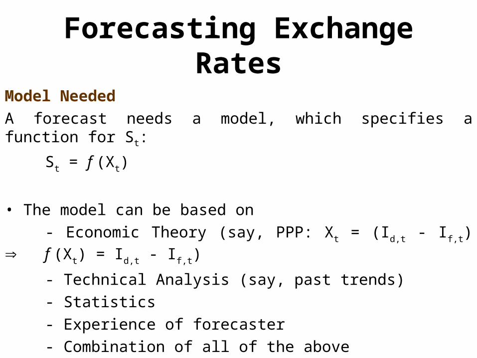
Model Needed

A forecast needs a model, which specifies a function for St:

St = f (Xt)

• The model can be based on

- Economic Theory (say, PPP: Xt = (Id,t - If,t) f (Xt) = Id,t - If,t)

- Technical Analysis (say, past trends)

- Statistics

- Experience of forecaster

- Combination of all of the above

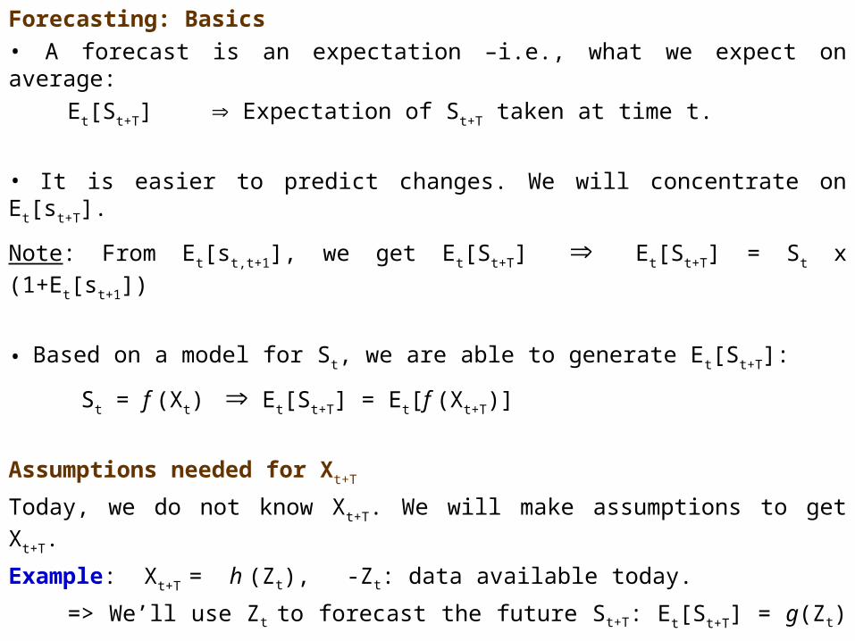
Forecasting: Basics

• A forecast is an expectation –i.e., what we expect on average:

Et[St+T] Expectation of St+T taken at time t.

• It is easier to predict changes. We will concentrate on Et[st+T].

Note: From Et[st,t+1], we get Et[St+T] Et[St+T] = St x (1+Et[st+1])

• Based on a model for St, we are able to generate Et[St+T]:

St = f (Xt) Et[St+T] = Et[f (Xt+T)]

Assumptions needed for Xt+T

Today, we do not know Xt+T. We will make assumptions to get Xt+T.

Example: Xt+T = h (Zt), -Zt: data available today.

=> We’ll use Zt to forecast the future St+T: Et[St+T] = g(Zt)

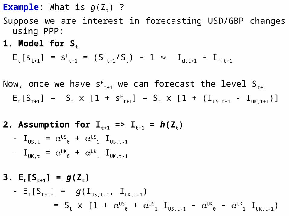
Example: What is g(Zt) ?

Suppose we are interest in forecasting USD/GBP changes using PPP:

1. Model for St

Et[st+1] = sFt+1 = (SF

t+1/St) - 1 Id,t+1 - If,t+1

Now, once we have sFt+1 we can forecast the level St+1

Et[St+1] = St x [1 + sFt+1] = St x [1 + (IUS,t+1 - IUK,t+1)]

2. Assumption for It+1 => It+1 = h(Zt)

- IUS,t = US0 + US

1 IUS,t-1

- IUK,t = UK0 + UK

1 IUK,t-1

3. Et[St+1] = g(Zt)

- Et[St+1] = g(IUS,t-1, IUK,t-1)

= St x [1 + US0 + US

1 IUS,t-1 - UK0 - UK

1 IUK,t-1)

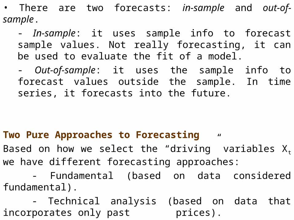
• There are two forecasts: in-sample and out-of-sample.

- In-sample: it uses sample info to forecast sample values. Not really forecasting, it can be used to evaluate the fit of a model.

- Out-of-sample: it uses the sample info to forecast values outside the sample. In time series, it forecasts into the future.

Two Pure Approaches to Forecasting

Based on how we select the “driving” variables Xt we have different forecasting approaches:

- Fundamental (based on data considered fundamental).

- Technical analysis (based on data that incorporates only past prices).

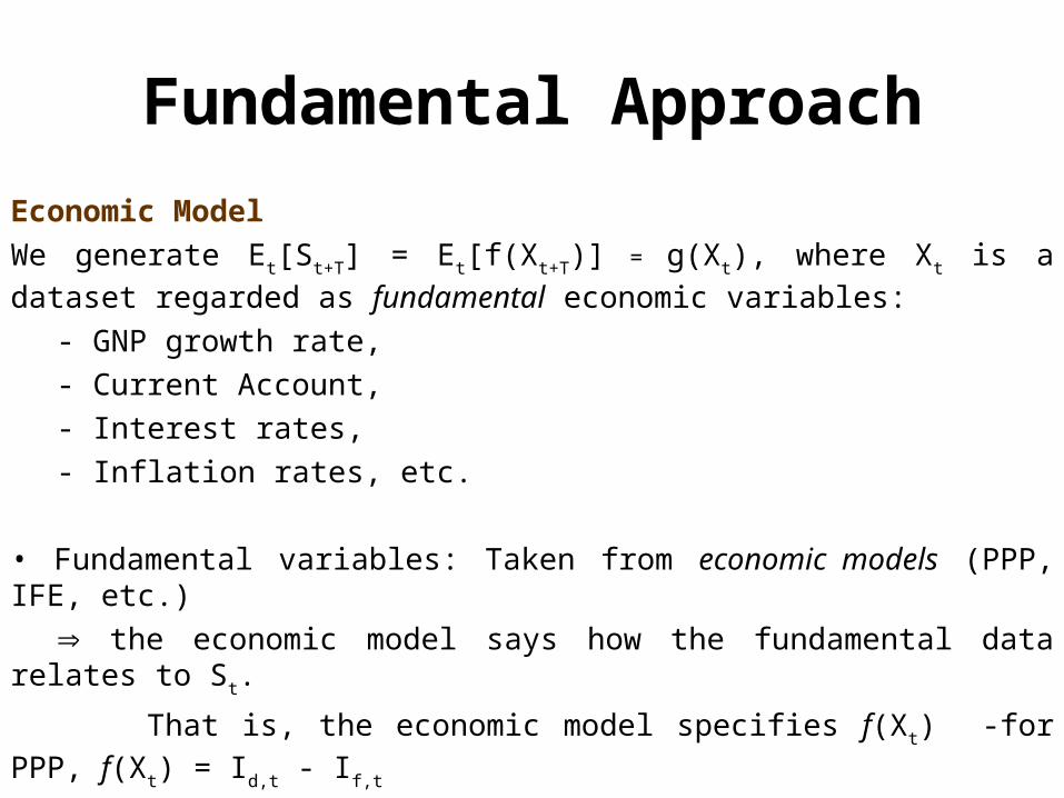
Fundamental Approach

Economic Model

We generate Et[St+T] = Et[f(Xt+T)] = g(Xt), where Xt is a dataset regarded

as fundamental economic variables:

- GNP growth rate,

- Current Account,

- Interest rates,

- Inflation rates, etc.

• Fundamental variables: Taken from economic models (PPP, IFE, etc.)

the economic model says how the fundamental data relates to St.

That is, the economic model specifies f(Xt) -for PPP, f(Xt) = Id,t - If,t

• The economic model usually incorporates:

- Statistical characteristics of the data (seasonality, etc.)

- Experience of the forecaster (what info to use, lags, etc.)

Mixture of art and science.

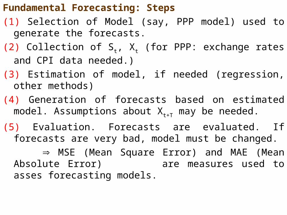
Fundamental Forecasting: Steps

(1) Selection of Model (say, PPP model) used to generate the forecasts.

(2) Collection of St, Xt (for PPP: exchange rates and CPI data needed.)

(3) Estimation of model, if needed (regression, other methods)

(4) Generation of forecasts based on estimated model. Assumptions about Xt+T may be needed.

(5) Evaluation. Forecasts are evaluated. If forecasts are very bad, model must be changed.

MSE (Mean Square Error) and MAE (Mean Absolute Error) are measures used to asses forecasting models.

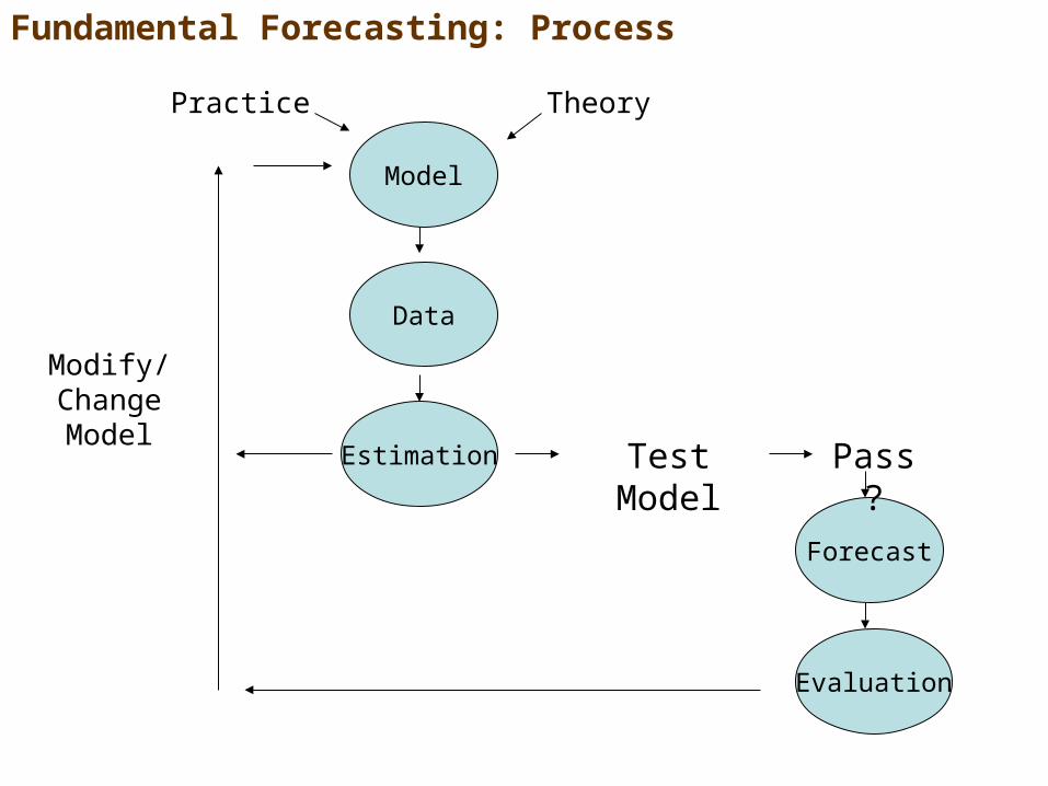
Fundamental Forecasting: Process

Model

Data

Estimation

Forecast

Evaluation

Modify/Change Model

Test Model

Theory

Pass?

Practice

Forecasting

0.0000

0.2000

0.4000

0.6000

0.8000

1.0000

1.2000Ja

n-99

Jul-9

9Ja

n-00

Jul-0

0

Jan-

01Ju

l-01

Jan-

02Ju

l-02

Jan-

03

Jul-0

3Ja

n-04

Jul-0

4Ja

n-05

Jul-0

5

Jan-

06Ju

l-06

Jan-

07Ju

l-07

Jan-

08Ju

l-08

Jan-

09Ju

l-09

Jan-

10

Jul-1

0

AUD/

USD

Estimation Period

Out-of-Sample Forecasts

Validation Forecasts

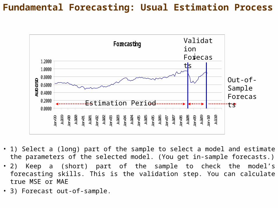
Fundamental Forecasting: Usual Estimation Process

• 1) Select a (long) part of the sample to select a model and estimate the parameters of the selected model. (You get in-sample forecasts.)

• 2) Keep a (short) part of the sample to check the model’s forecasting skills. This is the validation step. You can calculate true MSE or MAE

• 3) Forecast out-of-sample.

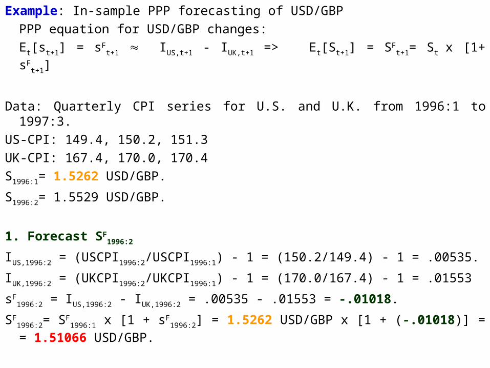
Example: In-sample PPP forecasting of USD/GBP

PPP equation for USD/GBP changes:

Et[st+1] = sFt+1 IUS,t+1 - IUK,t+1 => Et[St+1] = SF

t+1= St x [1+ sFt+1]

Data: Quarterly CPI series for U.S. and U.K. from 1996:1 to 1997:3.

US-CPI: 149.4, 150.2, 151.3

UK-CPI: 167.4, 170.0, 170.4

S1996:1= 1.5262 USD/GBP.

S1996:2= 1.5529 USD/GBP.

1. Forecast SF1996:2

IUS,1996:2 = (USCPI1996:2/USCPI1996:1) - 1 = (150.2/149.4) - 1 = .00535.

IUK,1996:2 = (UKCPI1996:2/UKCPI1996:1) - 1 = (170.0/167.4) - 1 = .01553

sF1996:2 = IUS,1996:2 - IUK,1996:2 = .00535 - .01553 = -.01018.

SF1996:2= SF

1996:1 x [1 + sF1996:2] = 1.5262 USD/GBP x [1 + (-.01018)] = =

1.51066 USD/GBP.

• Example (continuation):

SF1996:2= 1.51066 USD/GBP.

2. Forecast evaluation (Forecast error: SF1996:2-S1996:2)

1996:2 = SF1996:2-S1996:2 = 1.51066 – 1.5529 = -0.0422.

For the whole sample:

MSE: [(-0.0422)2 + (-0.0471)2 + .... + (-0.1259)2]/6 = 0.017063278

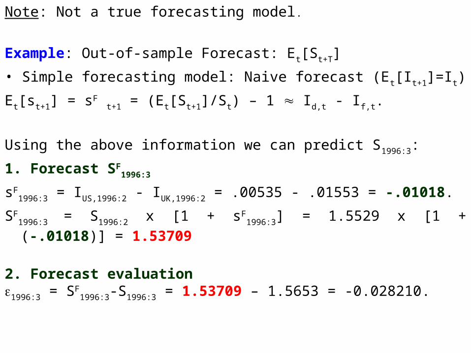
Note: Not a true forecasting model.

Example: Out-of-sample Forecast: Et[St+T]

• Simple forecasting model: Naive forecast (Et[It+1]=It)

Et[st+1] = sF t+1 = (Et[St+1]/St) – 1 Id,t - If,t.

Using the above information we can predict S1996:3:

1. Forecast SF1996:3

sF1996:3 = IUS,1996:2 - IUK,1996:2 = .00535 - .01553 = -.01018.

SF1996:3 = S1996:2 x [1 + sF

1996:3] = 1.5529 x [1 + (-.01018)] = 1.53709

2. Forecast evaluation1996:3 = SF

1996:3-S1996:3 = 1.53709 – 1.5653 = -0.028210.

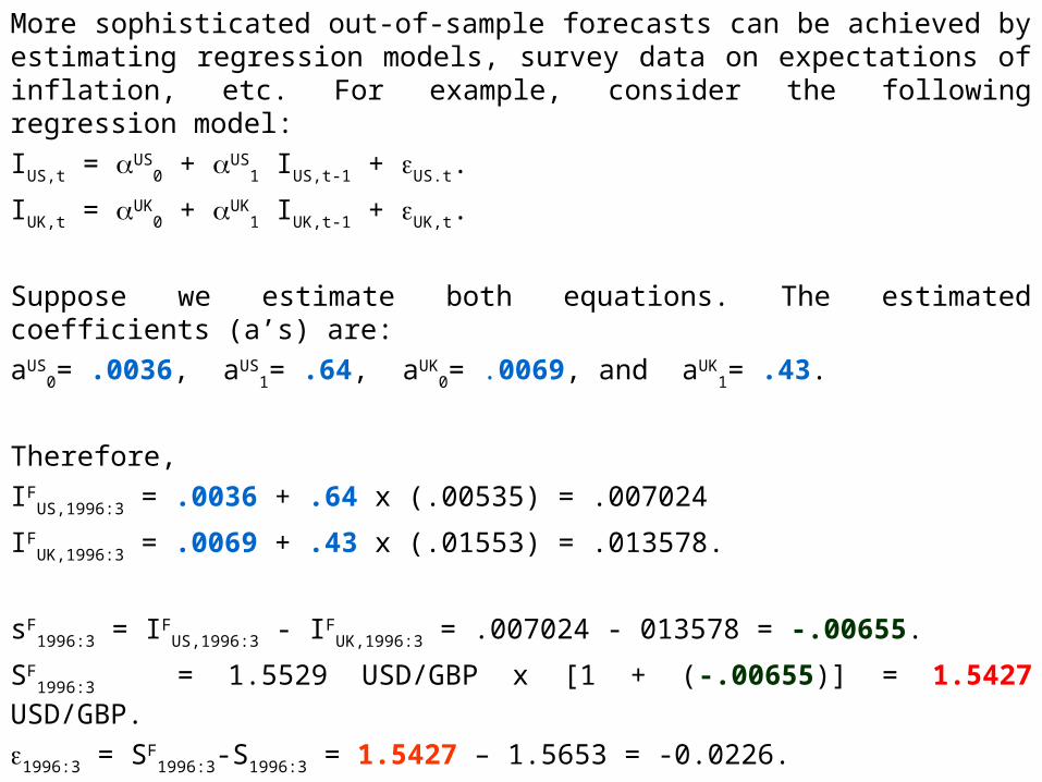
More sophisticated out-of-sample forecasts can be achieved by estimating regression models, survey data on expectations of inflation, etc. For example, consider the following regression model:

IUS,t = US0 + US

1 IUS,t-1 + US.t.

IUK,t = UK0 + UK

1 IUK,t-1 + UK,t.

Suppose we estimate both equations. The estimated coefficients (a’s) are:

aUS0= .0036, aUS

1= .64, aUK0= .0069, and aUK

1= .43.

Therefore,

IFUS,1996:3 = .0036 + .64 x (.00535) = .007024

IFUK,1996:3 = .0069 + .43 x (.01553) = .013578.

sF1996:3 = IF

US,1996:3 - IF

UK,1996:3 = .007024 - 013578 = -.00655.

SF1996:3 = 1.5529 USD/GBP x [1 + (-.00655)] = 1.5427 USD/GBP.

1996:3 = SF1996:3-S1996:3 = 1.5427 – 1.5653 = -0.0226.

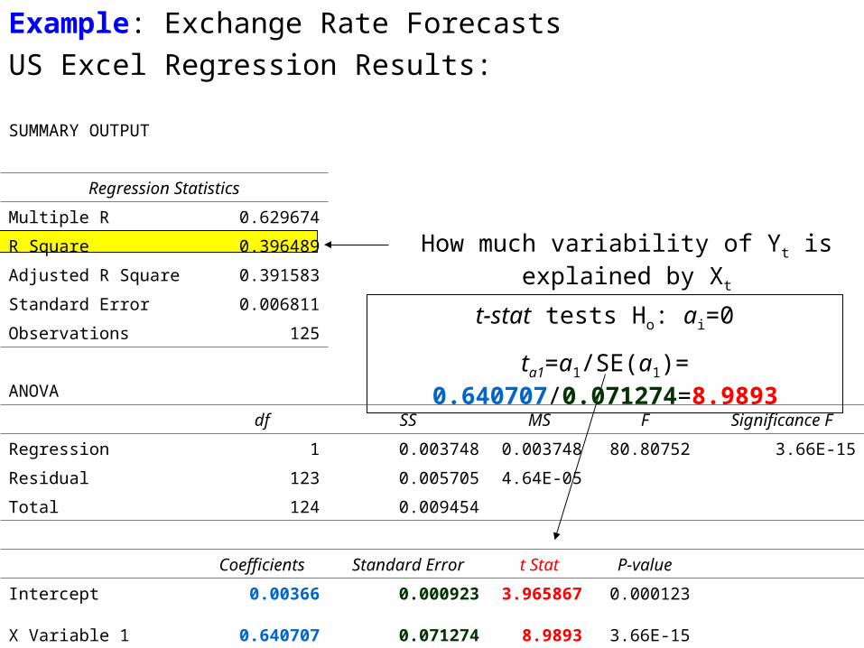
Example: Exchange Rate Forecasts

US Excel Regression Results:

How much variability of Yt is explained by Xt

t-stat tests Ho: ai=0

ta1=a1/SE(a1)= 0.640707/0.071274=8.9893

SUMMARY OUTPUT

Regression Statistics

Multiple R 0.629674

R Square 0.396489

Adjusted R Square 0.391583

Standard Error 0.006811

Observations 125

ANOVA

  df SS MS F Significance F

Regression 1 0.003748 0.003748 80.80752 3.66E-15

Residual 123 0.005705 4.64E-05

Total 124 0.009454      

  Coefficients Standard Error t Stat P-value  

Intercept 0.00366 0.000923 3.965867 0.000123

X Variable 1 0.640707 0.071274 8.9893 3.66E-15  

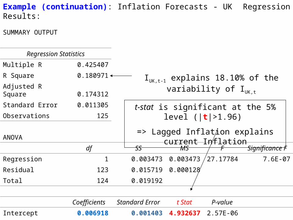
Example (continuation): Inflation Forecasts - UK Regression Results:

SUMMARY OUTPUT

Regression Statistics

Multiple R 0.425407

R Square 0.180971

Adjusted R Square 0.174312

Standard Error 0.011305

Observations 125

ANOVA

  df SS MS F Significance F

Regression 1 0.003473 0.003473 27.17784 7.6E-07

Residual 123 0.015719 0.000128

Total 124 0.019192      

  Coefficients Standard Error t Stat P-value  

Intercept 0.006918 0.001403 4.932637 2.57E-06

X Variable 1 0.428132 0.082124 5.213237 7.6E-07  

IUK,t-1 explains 18.10% of the variability of IUK,t

t-stat is significant at the 5% level (|t|>1.96)

=> Lagged Inflation explains current Inflation

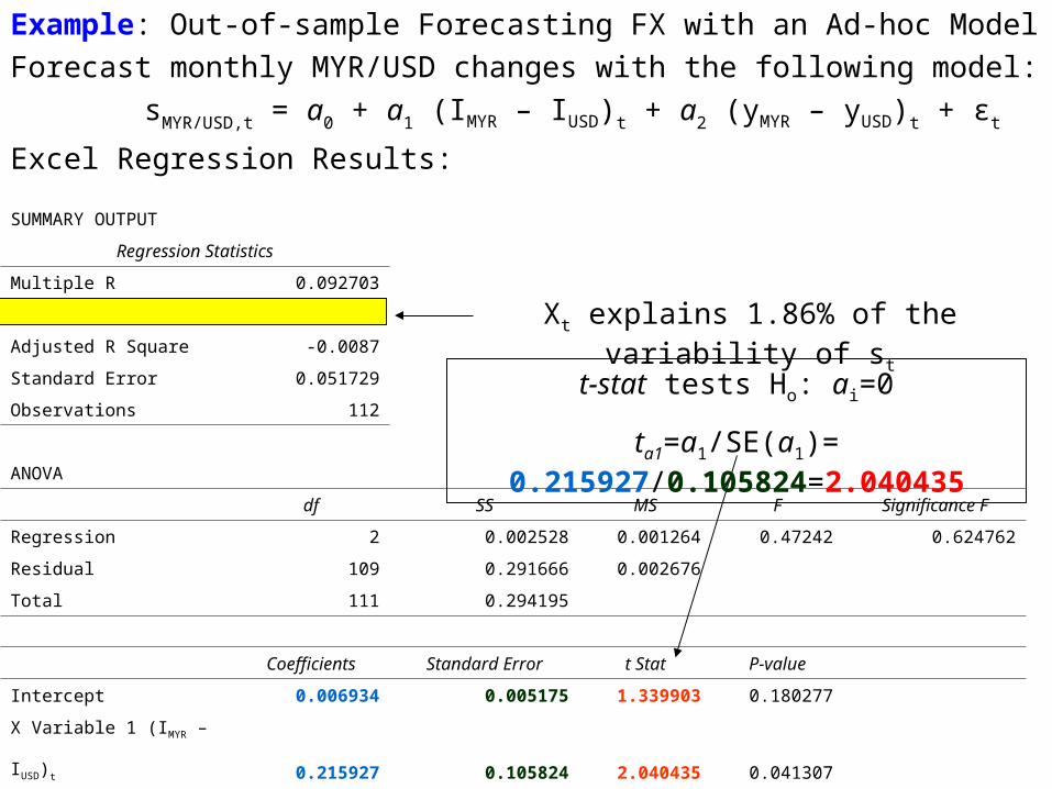
Example: Out-of-sample Forecasting FX with an Ad-hoc Model

Forecast monthly MYR/USD changes with the following model:

sMYR/USD,t = a0 + a1 (IMYR – IUSD)t + a2 (yMYR – yUSD)t + εt

Excel Regression Results:

SUMMARY OUTPUT

Regression Statistics

Multiple R 0.092703

R Square 0.018594

Adjusted R Square -0.0087

Standard Error 0.051729

Observations 112

ANOVA

  df SS MS F Significance F

Regression 2 0.002528 0.001264 0.47242 0.624762

Residual 109 0.291666 0.002676

Total 111 0.294195      

  Coefficients Standard Error t Stat P-value  

Intercept 0.006934 0.005175 1.339903 0.180277

X Variable 1 (IMYR – IUSD)t 0.215927 0.105824 2.040435 0.041307

X Variable 2 (yMYR – yUSD)t 0.091592 0.051676 1.772428 0.076326  

Xt explains 1.86% of the variability of st

t-stat tests Ho: ai=0

ta1=a1/SE(a1)= 0.215927/0.105824=2.040435

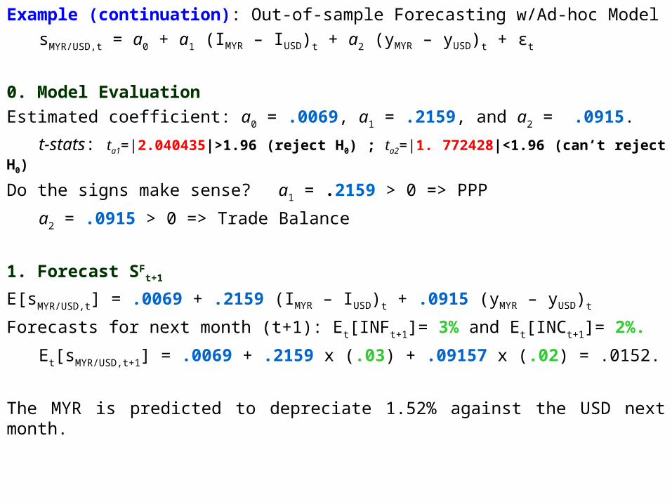
Example (continuation): Out-of-sample Forecasting w/Ad-hoc Model

sMYR/USD,t = a0 + a1 (IMYR – IUSD)t + a2 (yMYR – yUSD)t + εt

0. Model Evaluation

Estimated coefficient: a0 = .0069, a1 = .2159, and a2 = .0915.

t-stats: ta1=|2.040435|>1.96 (reject H0) ; ta2=|1. 772428|<1.96 (can’t reject H0)

Do the signs make sense? a1 = .2159 > 0 => PPP

a2 = .0915 > 0 => Trade Balance

1. Forecast SFt+1

E[sMYR/USD,t] = .0069 + .2159 (IMYR – IUSD)t + .0915 (yMYR – yUSD)t

Forecasts for next month (t+1): Et[INFt+1]= 3% and Et[INCt+1]= 2%.

Et[sMYR/USD,t+1] = .0069 + .2159 x (.03) + .09157 x (.02) = .0152.

The MYR is predicted to depreciate 1.52% against the USD next month.

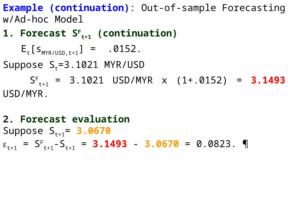
Example (continuation): Out-of-sample Forecasting w/Ad-hoc Model

1. Forecast SFt+1 (continuation)

Et[sMYR/USD,t+1] = .0152.

Suppose St=3.1021 MYR/USD

SFt+1 = 3.1021 USD/MYR x (1+.0152) = 3.1493 USD/MYR.

2. Forecast evaluationSuppose St+1= 3.0670t+1 = SF

t+1-St+1 = 3.1493 - 3.0670 = 0.0823. ¶

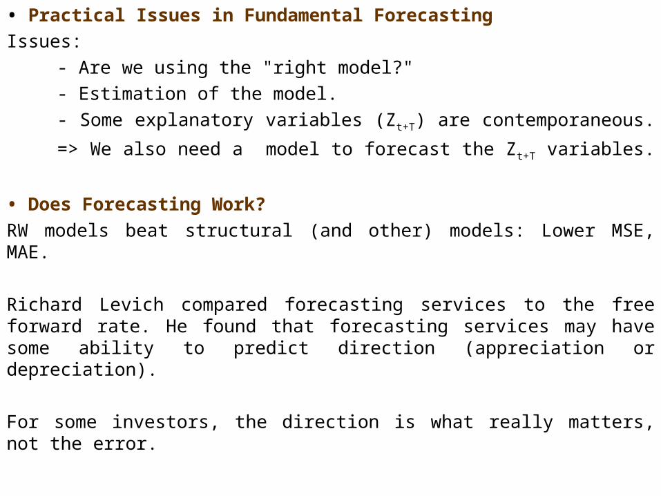
• Practical Issues in Fundamental Forecasting

Issues:

- Are we using the "right model?"

- Estimation of the model.

- Some explanatory variables (Zt+T) are contemporaneous.

=> We also need a model to forecast the Zt+T variables.

• Does Forecasting Work?

RW models beat structural (and other) models: Lower MSE, MAE.

Richard Levich compared forecasting services to the free forward rate. He found that forecasting services may have some ability to predict direction (appreciation or depreciation).

For some investors, the direction is what really matters, not the error.

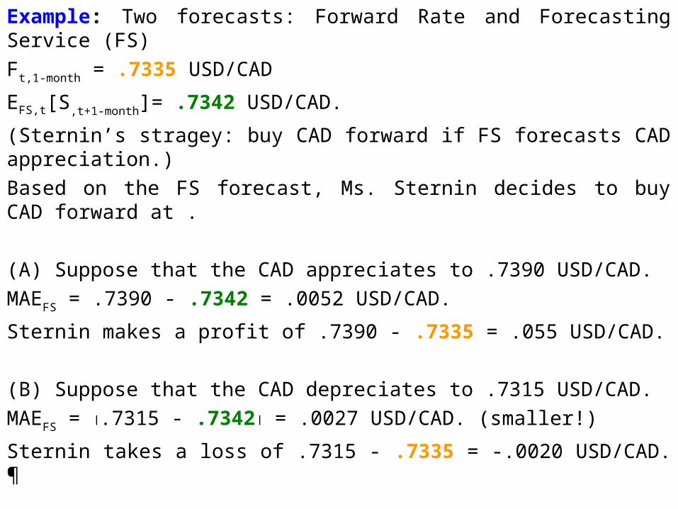
Example: Two forecasts: Forward Rate and Forecasting Service (FS)

Ft,1-month = .7335 USD/CAD

EFS,t[S,t+1-month]= .7342 USD/CAD.

(Sternin’s stragey: buy CAD forward if FS forecasts CAD appreciation.)

Based on the FS forecast, Ms. Sternin decides to buy CAD forward at .

(A) Suppose that the CAD appreciates to .7390 USD/CAD.

MAEFS = .7390 - .7342 = .0052 USD/CAD.

Sternin makes a profit of .7390 - .7335 = .055 USD/CAD.

(B) Suppose that the CAD depreciates to .7315 USD/CAD.

MAEFS = .7315 - .7342 = .0027 USD/CAD. (smaller!)

Sternin takes a loss of .7315 - .7335 = -.0020 USD/CAD. ¶

Technical Analysis Approach

• Based on a small set of the available data: past price information.

• TA looks for the repetition of specific price patterns.

Discovering these patterns is an art, not a science.

• TA attempts to generate signals: trends and turning points.

• Popular models:

- Moving Averages (MA)

- Filters

- Momentum indicators.

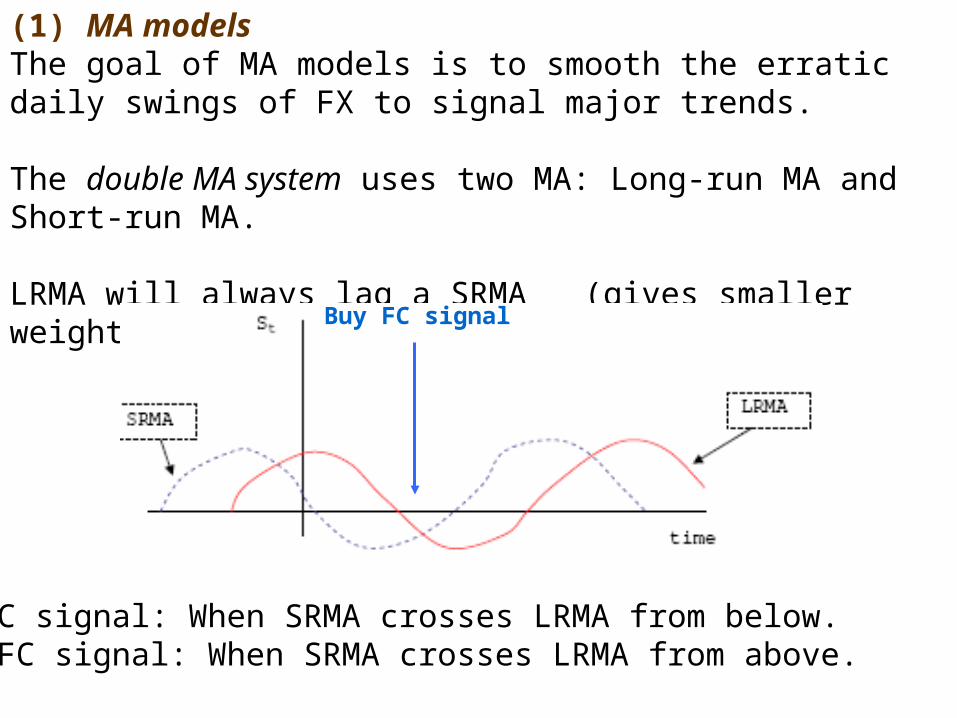
(1) MA modelsThe goal of MA models is to smooth the erratic daily swings of FX to signal major trends.

The double MA system uses two MA: Long-run MA and Short-run MA. LRMA will always lag a SRMA (gives smaller weights to recent St).

Buy FC signal: When SRMA crosses LRMA from below.Sell FC signal: When SRMA crosses LRMA from above.

Buy FC signal

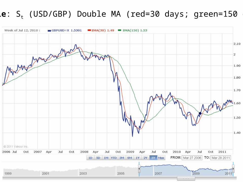
Example: St (USD/GBP) Double MA (red=30 days; green=150 days)

(2) Filter models The filter, X, is a percentage that helps a trader forecasts a trend.

Buy signal: when St rises X% above its most recent trough.

Sell signal: when St falls X% below the previous peak.

Idea: When St reaches a peak Sell FC

When St reaches a trough Buy FC.

Key: Identifying the peak or trough. We use the filter to do it:

When St moves X% above (below) its most recent peak (trough), we

have a trading signal.

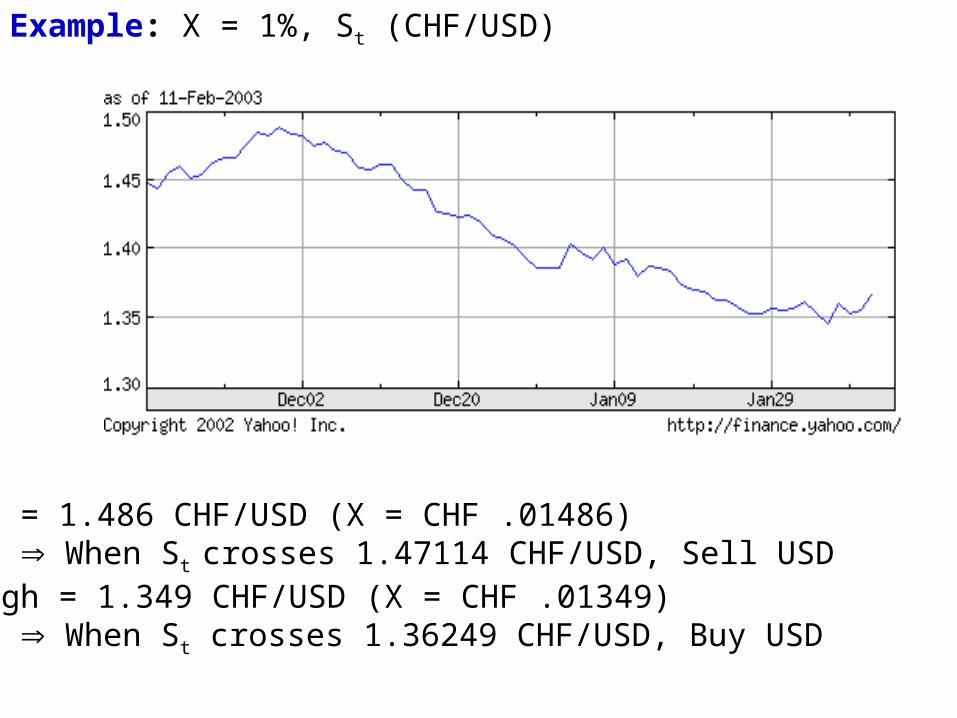
Example: X = 1%, St (CHF/USD)

Peak = 1.486 CHF/USD (X = CHF .01486) When St crosses 1.47114 CHF/USD, Sell USD

Trough = 1.349 CHF/USD (X = CHF .01349) When St crosses 1.36249 CHF/USD, Buy USD

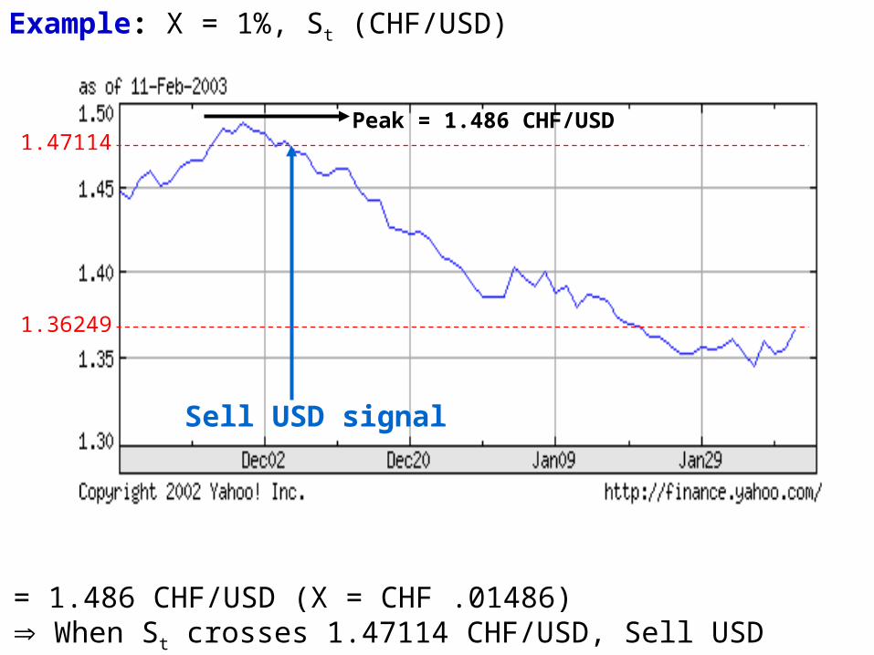
Example: X = 1%, St (CHF/USD)

Peak = 1.486 CHF/USD (X = CHF .01486) When St crosses 1.47114 CHF/USD, Sell USD

1.47114

Sell USD signal

1.36249

Peak = 1.486 CHF/USD

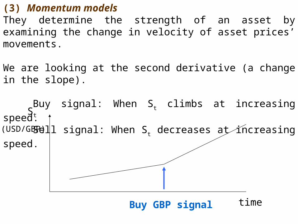
(3) Momentum modelsThey determine the strength of an asset by examining the change in velocity of asset prices’ movements.

We are looking at the second derivative (a change in the slope).

Buy signal: When St climbs at increasing speed.

Sell signal: When St decreases at increasing speed.

(USD/GBP)

time

St

Buy GBP signal

• TA Summary:TA models monitor the derivative (slope) of a time series graph. Signals are generated when the slope varies significantly.

• Technical Approach: Evidence• RW model: seems to be a very good forecasting model.

• Many economists have a negative view of TA: TA runs against market efficiency (see RC).

• Informal empirical evidence for TA:The marketplace is full of newsletters and consultants selling technical analysis forecasts and predictions.

• Some academic support: Bilson points out that linear comparisons -i.e., based on correlations- are meaningless, since TA rely on non-linearities. Bilson, based on non-linear models, finds weak support for TA.

Exchange Rate Volatility

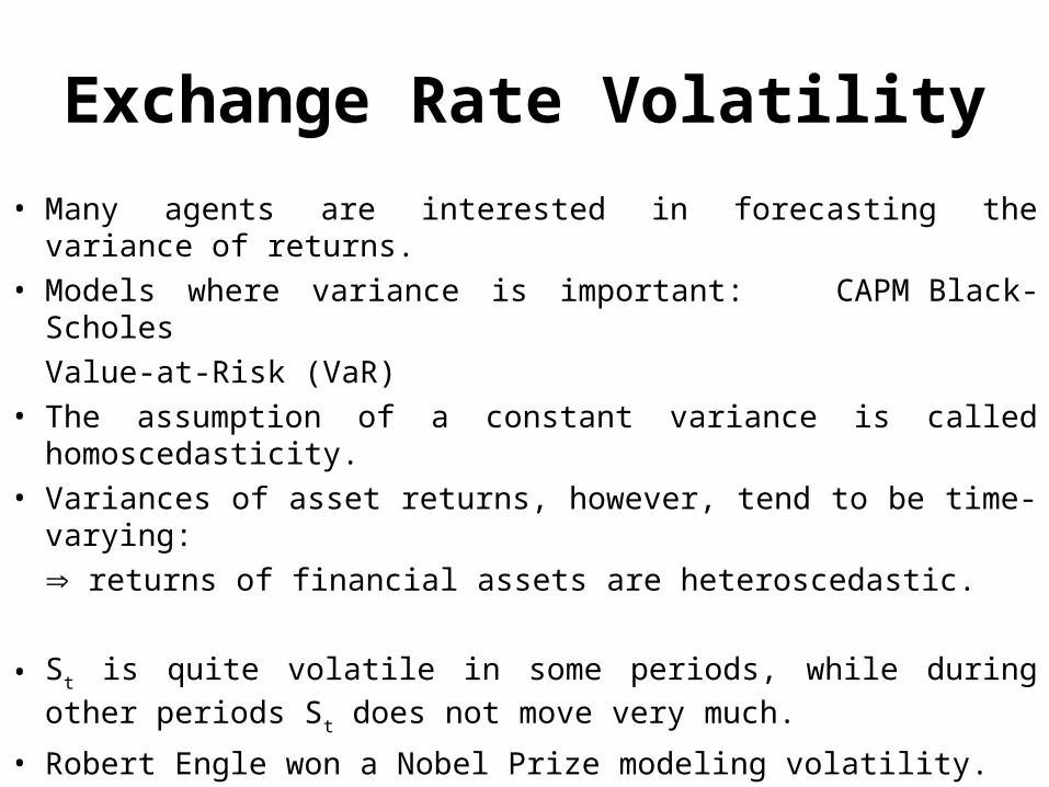
• Many agents are interested in forecasting the variance of returns.

• Models where variance is important: CAPMBlack-Scholes

Value-at-Risk (VaR)

• The assumption of a constant variance is called homoscedasticity.

• Variances of asset returns, however, tend to be time-varying:

returns of financial assets are heteroscedastic.

• St is quite volatile in some periods, while during other periods St does

not move very much. • Robert Engle won a Nobel Prize modeling volatility.

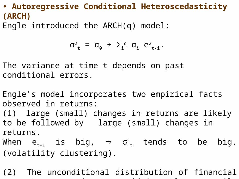
• Autoregressive Conditional Heteroscedasticity (ARCH)Engle introduced the ARCH(q) model:

σ2t = α0 + Σi

q αi e2

t-i.

The variance at time t depends on past conditional errors.

Engle's model incorporates two empirical facts observed in returns:(1) large (small) changes in returns are likely to be followed by

large (small) changes in returns. When et-1 is big, σ2

t tends to be big. (volatility clustering).

(2) The unconditional distribution of financial assets' returns has thicker (fatter) tails than the normal distribution.

Example: Volatility clustering and fat tails is observed in time series plots and histograms of the USD/GBP. ¶

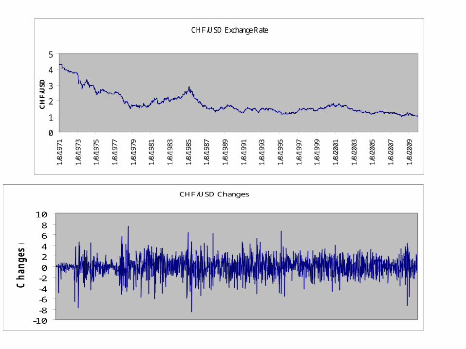
CHF/USD Exchange Rate

0

1

2

3

4

51/

8/19

71

1/8/

1973

1/8/

1975

1/8/

1977

1/8/

1979

1/8/

1981

1/8/

1983

1/8/

1985

1/8/

1987

1/8/

1989

1/8/

1991

1/8/

1993

1/8/

1995

1/8/

1997

1/8/

1999

1/8/

2001

1/8/

2003

1/8/

2005

1/8/

2007

1/8/

2009

CH

F/U

SD

CHF/USD Changes

-10-8-6-4-202468

10

Ch

an

ges

(%)

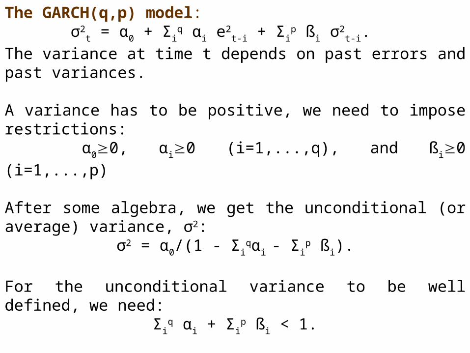
The GARCH(q,p) model:σ2

t = α0 + Σiq αi e

2t-i + Σi

p ßi σ2

t-i.

The variance at time t depends on past errors and past variances.

A variance has to be positive, we need to impose restrictions: α00, αi0 (i=1,...,q), and ßi0 (i=1,...,p)

After some algebra, we get the unconditional (or average) variance, σ2:

σ2 = α0/(1 - Σiqαi - Σi

p ßi).

For the unconditional variance to be well defined, we need:Σi

q αi + Σip ßi < 1.

• GARCH models have been successfully employed for exchange rates.

Empirical regularity: A GARCH(1,1) model tends to work well:σ2

t = α0 + α1 e2

t-1 + ß1 σ2

t-1.

σ2 is well defined when λ=α1+ß1<1.

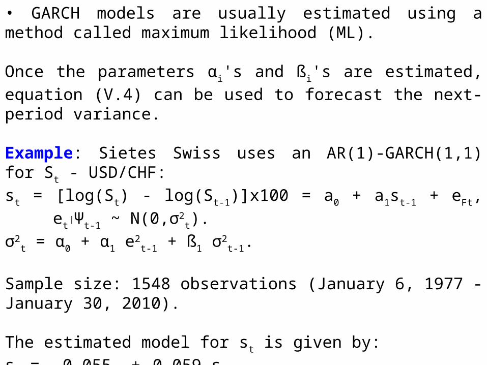
• GARCH models are usually estimated using a method called maximum likelihood (ML).

Once the parameters αi's and ßi's are estimated, equation (V.4) can be

used to forecast the next-period variance.

Example: Sietes Swiss uses an AR(1)-GARCH(1,1) for St - USD/CHF:

st = [log(St) - log(St-1)]x100 = a0 + a1st-1 + eFt, etΨt-1 ~ N(0,σ2t).

σ2t = α0 + α1 e

2t-1 + ß1 σ

2t-1.

Sample size: 1548 observations (January 6, 1977 - January 30, 2010).

The estimated model for st is given by:

st = -0.055 + 0.059 st-1,

(1.10) (1.78)σ2

t = 0.140 + 0.079 e2t-1 + 0.876 σ2

t-1.

(2.19) (4.16) (25.95)Note: λ=.955 < 1.

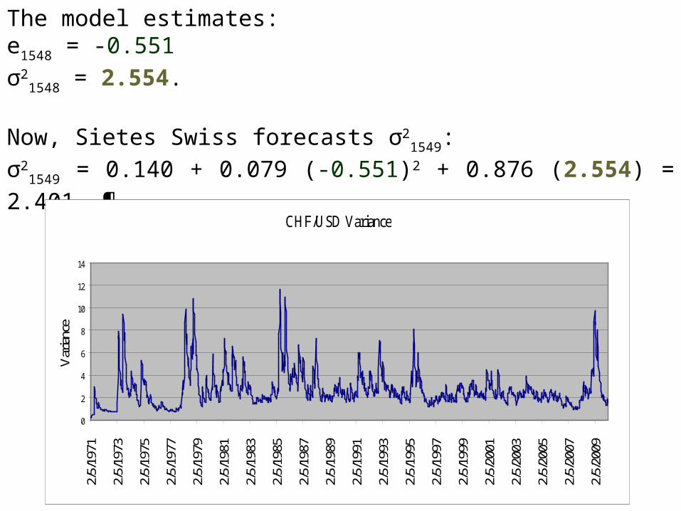
The model estimates:e1548 = -0.551

σ21548 = 2.554.

Now, Sietes Swiss forecasts σ21549:

σ21549 = 0.140 + 0.079 (-0.551)2 + 0.876 (2.554) = 2.401. ¶

CHF/USD Variance

0

2

4

6

8

10

12

14

2/5/

1971

2/5/

1973

2/5/

1975

2/5/

1977

2/5/

1979

2/5/

1981

2/5/

1983

2/5/

1985

2/5/

1987

2/5/

1989

2/5/

1991

2/5/

1993

2/5/

1995

2/5/

1997

2/5/

1999

2/5/

2001

2/5/

2003

2/5/

2005

2/5/

2007

2/5/

2009

Var

ianc

e

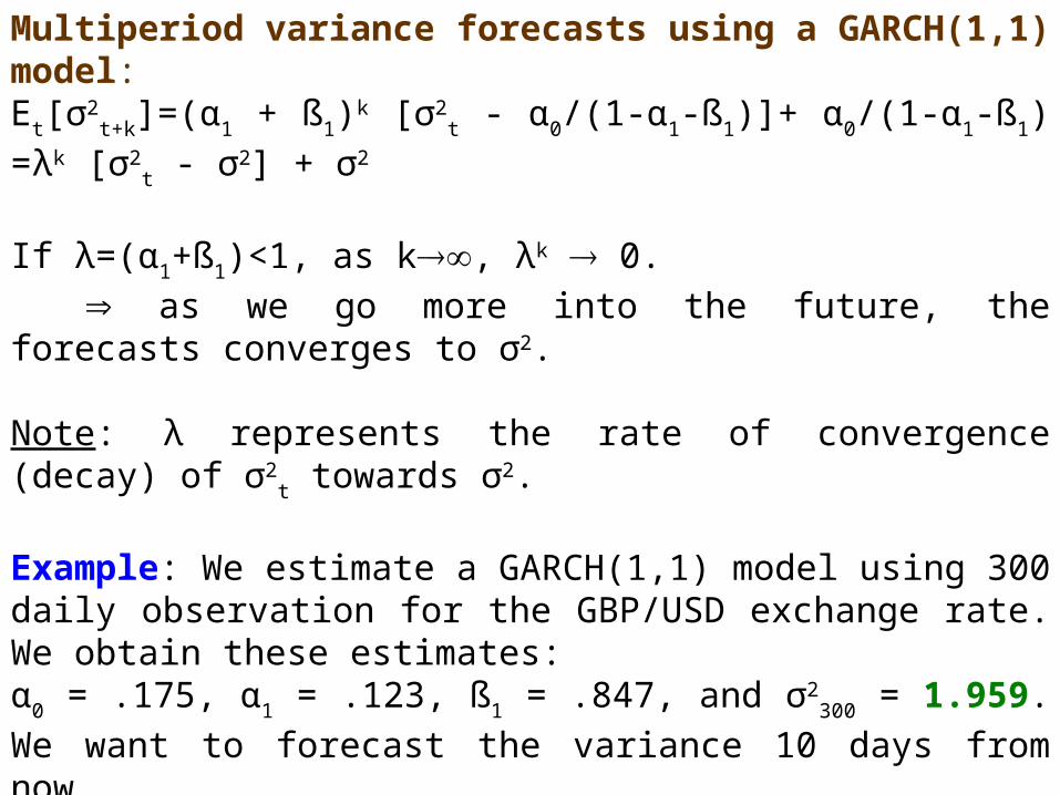
Multiperiod variance forecasts using a GARCH(1,1) model: Et[σ

2t+k]=(α1 + ß1)

k [σ2t - α0/(1-α1-ß1)]+ α0/(1-α1-ß1) =λk [σ2

t - σ2] + σ2

If λ=(α1+ß1)<1, as k, λk 0.

as we go more into the future, the forecasts converges to σ2. Note: λ represents the rate of convergence (decay) of σ2

t towards σ2.

Example: We estimate a GARCH(1,1) model using 300 daily observation for the GBP/USD exchange rate. We obtain these estimates:α0 = .175, α1 = .123, ß1 = .847, and σ2

300 = 1.959.

We want to forecast the variance 10 days from now.

The unconditional variance is σ2 = .175/(1 - .123 - .847) = 5.833.

The 10-day-ahead variance forecast is:E300[σ

2310] = (.97)10 [ 1.959 - 5.833] + 5.833 = 2.976.

the volatility forecast 10 days ahead is σ310 = 1.725%. ¶

J.P. Morgan's RiskMetrics ApproachIn October 1994, J.P. Morgan unveiled its risk management software.

RiskMetrics is a method that estimates the market risk of a portfolio, using the Value-at-Risk (VAR) approach. RiskMetrics uses a simple specification to model σ2

t:

σ2t = (1-γ) e2

t-1 + γ σ2t-1.

next period's variance is a weighted average of this period's squared forecast error and this period's variance.

RiskMetrics approach involves an IGARCH model: α0=0

γ = (1-α1) = ß1.

J.P. Morgan set: γ=.94, for daily data. γ=.97, for monthly volatility.

Given the large number of series that J.P. Morgan uses (more than 500), RiskMetrics uses the same γ for all the series.

Example: Suppose we estimate a time-varying variance with the RiskMetrics model using 300 daily observations for GBP/USD.

Estimates σ2300 = 1.959 and e300 = 0.663.

Forecast for the variance tomorrow:E300[σ

2301] = (.94) 1.959 + .06 (.633)2 = 1.8655

That is, the volatility forecast for tomorrow is E300[σ301] = 1.366%. ¶