forecasting intra-day volatility. multiplicative component
TRANSCRIPT
UNIVERSITY OF AMSTERDAM
FACULTY OF ECONOMICS AND BUSSINESS
Master thesis
in the subject of
Financial Econometrics
Forecasting intra-day volatility.Multiplicative Component Realized GARCH
Karolina Jerofejevaite
10603484
Supervised by Peter Boswijk
2014.08.25
CONTENTS CONTENTS
Contents
1 Introduction 3
2 Literature review 5
3 Econometric methods 7
3.1 Multiplicative Component GARCH . . . . . . . . . . . . . . . . . . . . . . . 8
3.2 Realized GARCH . . . . . . . . . . . . . . . . . . . . . . . . . . . . . . . . . 9
3.2.1 Specification of the log-linear Realized GARCH(1,1) . . . . . . . . . . 12
3.2.2 Log-likelihood . . . . . . . . . . . . . . . . . . . . . . . . . . . . . . . 12
3.2.3 Multi-period Forecast . . . . . . . . . . . . . . . . . . . . . . . . . . . 13
3.2.4 Realized measures . . . . . . . . . . . . . . . . . . . . . . . . . . . . . 13
4 Data 16
5 Results 18
5.1 Realized GARCH modelling results . . . . . . . . . . . . . . . . . . . . . . . 18
5.2 Realized GARCH forecasting results . . . . . . . . . . . . . . . . . . . . . . 22
5.3 Modelling results for Multiplicative Component GARCH . . . . . . . . . . . 24
5.4 Forecasting results for Multiplicative Component GARCH . . . . . . . . . . 25
6 Possible extensions 31
6.1 Asymmetries . . . . . . . . . . . . . . . . . . . . . . . . . . . . . . . . . . . 31
6.2 Long memory . . . . . . . . . . . . . . . . . . . . . . . . . . . . . . . . . . . 34
7 Limitations 37
8 Conclusions 40
A Appendix 43
A.1 15 minute Realized Kernel calculation . . . . . . . . . . . . . . . . . . . . . . 43
A.2 Diebold-Mariano test for Comparing Predictive Accuracy . . . . . . . . . . . 43
A.3 Data analysis for Microsoft stock . . . . . . . . . . . . . . . . . . . . . . . . 44
1

CONTENTS CONTENTS
A.4 Results for Microsoft stock . . . . . . . . . . . . . . . . . . . . . . . . . . . . 46
A.4.1 Realized GARCH results . . . . . . . . . . . . . . . . . . . . . . . . . 46
A.4.2 Multiplicative Component GARCH results . . . . . . . . . . . . . . . 48
2

1 INTRODUCTION
1 Introduction
Up to date there is a huge amount of literature on modelling and forecasting daily variance
of the returns whereas intra-day volatility models are far less discussed. However, every year
trading becomes more and more frequent and automated. This motivates the development of
the intra-day volatility forecasting models. These forecasts then serve as an important part
of the algorithm for the schedule trades, asset pricing, changing hedge ratio. Also they help
place limit orders and can be used to calculate intra-day Value at Risk (VaR) which may
lead to allocation of the funds within a day. Consequently, interest in modelling intra-day
variance is growing.
Thus my main goal in this thesis is to try to find the most empirically suitable approach to
model and forecast intra-day variance. One of the most influential papers on this matter was
recently published by Engle and Sokalska (2012). The authors introduce the Multiplicative
Component GARCH model for High-frequency intra-day financial returns, which specifies
the conditional variance to be a product of daily, diurnal and stochastic intra-day volatility.
My master thesis builds on this paper. I investigate the performance of the mentioned vari-
ance components and I seek to answer the question - how significant are these components
for the intra-day volatility modelling and forecasting results?
In the mentioned paper commercially available volatility forecasts are used as a daily vari-
ance component. These predictions are made on the basis of a multi-factor risk model. In
contrast, I want to make use of information that high frequency data provides. Thus I take
a different approach and model the daily volatility component by Realized GARCH, intro-
duced by Hansen, Huang and Shek (2011). By the structure of the model, it accounts for
asymmetry and long memory properties of the daily returns. Also it has been proven that
the model gives substantial improvements for the daily conditional variance modelling and
forecasting over usual GARCH models. Standard GARCH models typically employ squared
returns to extract information about the current level of daily volatility. Within Realized
GARCH model, the observed realized measures of the latent volatility are used instead.
3

1 INTRODUCTION
These measures are build using high frequency returns in such a way that they approximate
the quadratic variation of the true underlying price process, by filtering out the microstruc-
ture noise. Overall, many realized measures have been proposed, in my work I focus on
5 minute Realized Variance, Sub-sampled 5 minute Realized Variance and Realized Kernel.
The last gives the most accurate daily forecasts among the three, therefore these forecasts are
then used as a daily variance component in the Multiplicative Component GARCH model.
After applying this model, I predict intra-day volatility 15 minutes ahead and use different
approaches to evaluate the obtained forecasts. That is, various true volatility proxies and
prediction measures are used. The models are applied to frequently traded stocks: Intel
Corporation and Microsoft. Data samples start on the 2nd of June, 1990 till the 3rd of May,
2011. Every trading day consists of 5 second log-returns. Thus in total there are 3000 days
of observations with 4680 5 second log-returns within each day.
This thesis is organized as follows. In the second chapter a literature review is given. In the
3rd chapter I introduce Realized GARCH and Multiplicative Component GARCH models.
The used data is detailed in Chapter 4. Obtained results are summarized in Chapter 5.
Possible extensions are discussed in Chapter 6. Limitations of the Realized GARCH model
are expressed in Chapter 7. Overall conclusions of the thesis are presented in Chapter 8.
4
2 LITERATURE REVIEW
2 Literature review
The frequency of trading in the financial markets is gradually increasing every year. We
find ourselves at the point where proper intra-day volatility model is of substantial empiri-
cal importance. It has been argued that conventional GARCH models are not suitable for
within-the-day modelling and fail to capture important features of the intra-day volatility.
(See for instance Andersen and Bollerslev (1997)). The reason for this is distinctive intra-
day seasonality or in other words diurnal patterns of the volatility. A number of closely
connected models were developed to take account of intra-day volatility patterns, see Ghose
and Kroner (1996), Andersen and Bollerslev (1997, 1998), Giot (2005) and Engle (2012).
The latter extended the model proposed by Andersen and Bollerslev (1997) and introduced
Multiplicative Component GARCH model. In contrast, to Andersen and Bollerslev, this
model included not only daily and diurnal volatility components but also a stochastic intra-
day component.
This thesis builds on the work of Engle and Sokalska (2012). The authors were dealing with
a huge amount of data (that is 2500 US equities with high frequency returns) thus the main
focus of their work was applying a number of different specifications and then comparing
forecasting results. Namely, they construct models for separate companies, pool data into
industries, and consider various criteria for grouping returns. And finally they arrive to the
conclusion that the forecasts from the pooled specifications outperform the corresponding
forecasts from company by company estimation. For this kind of modelling you need to have
an access to a comprehensive sample plus an extremely fast computer. Thus in my thesis I
take a different approach and focus on investigating the significance of the daily, diurnal and
a stochastic intra-day volatility components for the forecasting results. Along with in-depth
investigation of the properties of the intra-day returns. Moreover, I apply different ways to
evaluate the accuracy of the forecasts.
For the time being let’s focus on the daily volatility (component) modelling. Commonly
standard GARCH models are used. Within the GARCH framework, daily returns (typically
5

2 LITERATURE REVIEW
squared returns) are employed to extract information about the current level of volatility,
and this information is used to form expectations about the next period’s volatility. But it
must be emphasized that squared returns only offer a weak signal about the current level of
volatility. Moreover, it is known that GARCH model is slow at ’catching up’ and it will take
many periods for the conditional variance (implied by the GARCH model) to reach its new
level, as discussed in Andersen (2003). Therefore, since I am dealing with high-frequency
financial data, it is necessary to take advantage of this additional information. A number of
realized measures of volatility, including Realized variance, bipower variation, the Realized
Kernel, and others (see Andersen and Bollerslev (1998), Andersen (2001), Barndorff-Nielsen
and Shephard, (2002, 2004, 2008), Hansen and Lunde (2006), Bandi and Russell (2008))
prove to be far more informative about the current level of volatility than is the squared
return. This makes realized measures very useful for modelling and forecasting future volatil-
ity. Andersen (2001), Barndorff-Nielsen and Shephard (2002) show that applying Realized
variance, a measure constructed by summing high frequency squared returns, improves the
understanding of time-varying variance and ability to forecast future volatility. Hansen and
Lunde (2006) carry out an in-depth analysis of the Realized variance and investigate its
upward-biasedness at high frequencies. Their work show that using 1 to 5 minute squared
returns for Realized variance measure give the optimal results. Barndorff-Nielsen,Hansen,
Lunde and Shephard expand this influential Realized variance literature by introducing Re-
alized Kernel. This non-negative estimator is robust to autocorrelation of the high-frequency
returns and has broadly the same form as a standard heteroskedasticity and autocorrelation
consistent (HAC) covariance matrix.
Engle (2002) introduced a model called GARCH-X, which is GARCH model that includes
a realized measure. However, within the GARCH-X framework the variation in the realized
measures are left unexplained, due to this GARCH-X models are called partial. Engle and
Gallo (2006) introduced the first ’complete’ model in this context. Their model specifies a
GARCH structure for each of the realized measures, so that an additional latent volatility
process is introduced for each realized measure in the model. The model by Engle and
Gallo (2006) is known as the multiplicative error model (MEM), because it builds on the
6

3 ECONOMETRIC METHODS
MEM structure proposed by Engle (2002). Another complete model is the HEAVY model
by Shephard and Sheppard (2010), which also incorporates at least two separate equations:
one for latent volatility and the other one for realized measure. Thus unlike the traditional
GARCH models, these models operate with multiple latent volatility processes. Another
example of a complete model was introduced by Hansen, Huang and Shek (2011) and is
called Realized GARCH. This model combines a GARCH structure for the returns with
an integrated model for the realized measures of volatility. Importantly, the authors show
statistical gains from incorporating realized measures in the volatility models. This is not
the only paper that illustrates the benefit of including the realized measures in the analysis.
Shephard and Sheppard (2010) show that when it comes to forecasting, HEAVY models
out-perform standard GARCH substantially, for both within the sample and out of sample
forecasts. From this it seems that HEAVY models would be a great pick for daily variance
component forecast. However, in this model latent volatility and realized measure equations
are estimated separately. And Shephard and Sheppard (2010) briefly mention that if the
information was pooled across the two equations it might bring more explanatory power for
the model. That is exactly what is done by Hansen, Huang and Shek (2011) in the Realized
GARCH model. Therefore in this thesis Realized GARCH is chosen to model and forecast
daily volatility.
In this Master thesis I combine arguably the best known practices to model intra-day and
daily volatility. Namely, the Multiplicative Component GARCH by Engle and Sokalska
(2012) for intra-day variance and the Realized GARCH for daily volatility (component)
forecasting. This way I obtain an extended model, called the Multiplicative Component
Realized GARCH.
3 Econometric methods
General notation. Every trading day is divided into a number of bins (time intervals) N,
j = 1, ..., N marks an index of the bin within a day and t = 1, ..., T denotes the index of a
trading day. Both things combined we get that {t, j} indicates the j-th bin on the t-th day.
7

3.1 Multiplicative Component GARCH 3 ECONOMETRIC METHODS
Dataset contains high-frequency 5 second log returns. This means that the size of the bin
is 5 seconds and there are 4680 such bins within each trading day. The 5 second log returns
are defined as:
rt,j = log
(St,j
St,j−1
),
where St,j denotes the stock price at time {t, j}.
Then the daily returns can be obtained as follows:
rt =4680∑j=1
rt,j.
Please recall that there are 4680 5 second bins within a day.
Throughout this thesis 15 minute returns will be used often. Therefore, to distinguish these
15 minute returns from high frequency 5 second returns, I choose to denote them as rt,i,
where i = 1, ..., 26 (each day has 26 15 minute bins).
3.1 Multiplicative Component GARCH
The Multiplicative component GARCH model for the intra-day financial returns specifies the
conditional variance to be a multiplicative product of daily, diurnal and stochastic intra-day
volatility. In this section I give the general specification of the model.
The intra-day returns rt,i are assumed to take the following form:
rt,i =√htsiqt,iεt,i, εt,i ∼ N(0, 1). (1)
Here ht is the daily volatility component, si is the diurnal variance pattern, εt,i is the error
term, and qt,i is the stochastic intra-day volatility component, with E(qt,i) = 1. In this
thesis I chose to use 15 minute returns. Modelling of Multiplicative GARCH breaks down
in 3 major parts.
(i) Daily volatility component ht needs to be modelled and predicted. For this purpose
Realized GARCH model, detailed in section 3.2, is used.
(ii) The deterministic diurnal pattern (si) has to be obtained.
In order to distinguish day seasonality, let’s first divide the 15 minute squared returns
8
3.2 Realized GARCH 3 ECONOMETRIC METHODS
by the daily variance component ht:
r2t,i
ht= siqt,iε
2t,i ⇒ E
[r2t,i
ht
]= siE[qt,i] = si.
This leads to the following estimator of si:
si =1
T
T∑1
r2t,i
ht. (2)
(iii) The intra-day returns must be normalized by daily (ht) and diurnal patterns (si):
zt,i =rt,i√htsi≈ √qt,iεt,i
These obtained normalized returnszt,i are now used in a GARCH(1,1) model for the
intra-day stochastic component qt,i:
qt,i = ω + αz2t,i−1 + βqt,i−1 (3)
where zt,i | Ft,i−1 ∼ N(0, qt,i).
Here Ft,i−1 is a σ-algebra containing all the 15 minute returns observed up to the current
time moment {t, i}. In more detail, Ft,i−1 = {r1,1, ..., r1,N , ..., rt−1,1, ..., rt−1,N , rt,1, ..., rt,i−1}
and N = 26. I apply a simple GARCH(1,1) for the stochastic component qt,i as is done in
the paper by Engle and Sosalska (2012). However, possible extensions of this model will be
discussed in Chapter 7.
3.2 Realized GARCH
In this part I introduce Realized GARCH model proposed by Hansen, Huang and Shek (2011)
and the applied realized measures. It will be assumed that E(rt | Ft−1) = 0, which is em-
pirically proven to be accurate assumption. Here the information set Ft−1 contains the high
frequency returns rj,t and the realized measures constructed from these returns, observed
up to day t − 1. That is, Ft−1 = {rt−1,1, ..., rt−1,N , rt−2,1, ..., rt−1,N,, r1,1, ..., r1,N , xt−1, ..., x1}
where N=4680 and xt−1 denotes the obtained realized measure. As mentioned rt are the
daily returns and t = 1, ..., T is the index of the day. The interest lies within the unobserved
9
3.2 Realized GARCH 3 ECONOMETRIC METHODS
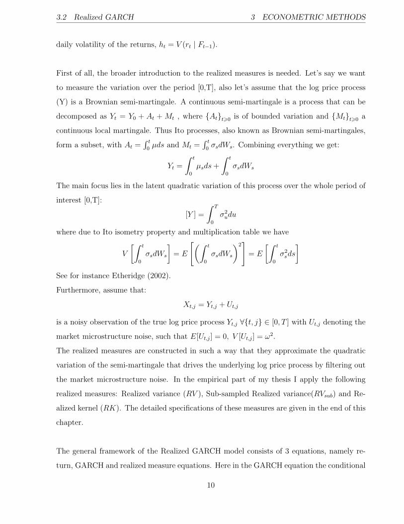
daily volatility of the returns, ht = V (rt | Ft−1).
First of all, the broader introduction to the realized measures is needed. Let’s say we want
to measure the variation over the period [0,T], also let’s assume that the log price process
(Y) is a Brownian semi-martingale. A continuous semi-martingale is a process that can be
decomposed as Yt = Y0 + At + Mt , where {At}t>0 is of bounded variation and {Mt}t>0 a
continuous local martingale. Thus Ito processes, also known as Brownian semi-martingales,
form a subset, with At =∫ t
0µds and Mt =
∫ t
0σsdWs. Combining everything we get:
Yt =
∫ t
0
µsds+
∫ t
0
σsdWs
The main focus lies in the latent quadratic variation of this process over the whole period of
interest [0,T]:
[Y ] =
∫ T
0
σ2udu
where due to Ito isometry property and multiplication table we have
V
[∫ t
0
σsdWs
]= E
[(∫ t
0
σsdWs
)2]
= E
[∫ t
0
σ2sds
]See for instance Etheridge (2002).
Furthermore, assume that:
Xt,j = Yt,j + Ut,j
is a noisy observation of the true log price process Yt,j ∀{t, j} ∈ [0, T ] with Ut,j denoting the
market microstructure noise, such that E[Ut,j] = 0, V [Ut,j] = ω2.
The realized measures are constructed in such a way that they approximate the quadratic
variation of the semi-martingale that drives the underlying log price process by filtering out
the market microstructure noise. In the empirical part of my thesis I apply the following
realized measures: Realized variance (RV ), Sub-sampled Realized variance(RVsub) and Re-
alized kernel (RK). The detailed specifications of these measures are given in the end of this
chapter.
The general framework of the Realized GARCH model consists of 3 equations, namely re-
turn, GARCH and realized measure equations. Here in the GARCH equation the conditional
10

3.2 Realized GARCH 3 ECONOMETRIC METHODS
variance ht depends not only on the ht−1 but also on the realized measure of the volatility,
denoted xt−1. Overall, the measurement equation is a very important component, that ties
the realized measure to the latent volatility. Also providing a simple way of modelling the
joint dependence between rt and xt. The specification of the model in more detail can be
found in section 3.2.1.
The authors Hansen, Huang and Shek (2011) define different specifications for the model,
however they do emphasize the choice of the log-linear Realized GARCH. There are few
reasons for this. First, log-linear specification automatically ensures a positive variance. In
practice the log-linear specification of the usual GARCH model is not often used because rt
may have a zero value and this would cause censoring in the model. In contrast, within the
Realized GARCH framework the logarithm of the returns (log(rt−1)) does not appear in the
model (this is explicitly shown below in equation (5)). For the motivation of not including
returns in the Realized GARCH model I refer the reader to the Hansen, Huang and Shek
(2011) paper. Another attractive feature of the log-linear Realized GARCH, is the fact that
it maintains the ARMA structure that characterizes some of the standard GARCH models.
All things considered, log-linear Realized GARCH seems like the best choice to be applied
in an empirical work.
Usually GARCH(1,1) specification is applied to account for the volatility clustering. Here I
am dealing with the returns of the Intel Corporation and Microsoft storcks. And GARCH(1,1)
proofs to be enough to correct for the serial autocorrelation in the residuals of the squared
residuals of the data analysed (detailed information about the data is provided in Chapter 4).
After taking in to account all of this argumentation, I chose to use log-linear Realized
GARCH(1,1) model for daily volatility modelling and forecasting. In the next section the
detailed specification of the model can be found.
11

3.2 Realized GARCH 3 ECONOMETRIC METHODS
3.2.1 Specification of the log-linear Realized GARCH(1,1)
Return equation:
rt =√htεt. (4)
GARCH equation:
ht = exp {ω + β log ht−1 + γ log xt−1} . (5)
Realized measure equation:
log xt = ξ + ϕ log ht + τ(εt) + ut. (6)
where τ(εt) = τ1εt + τ2(ε2t − 1) is a leverage effect such that E[τ(εt)] = 0 and ε ∼ iidN(0, 1),
u ∼ iidN(0, σ2u) and xt is a realized measure. It is shown in the paper by Hansen, Huang
and Shek (2011) that the use of this type of leverage equation τ(εt) in the realized measure
equation (6) induces EGARCH type structure in the GARCH equation (5).
From the model specification above another argument for choosing log-linear Realized GARCH
can be spotted. It lies within rt specification in equation (4). Which implies that:
log(r2t ) = log(ht) + log(ε2t )
and a realized measure is in many ways similar to the squared return, r2t , although a more
accurate measure of ht. Therefore, it is natural to express realized measure log(xt) in terms
of log(ht) and εt like in equation(6).
3.2.2 Log-likelihood
For the purpose of estimation, the Gaussian specification will be adopted, so that the log-
likelihood is given by:
l(r, x, θ) = −1
2
n∑t=1
(log(ht) +
r2t
ht+ log(σ2
u) +u2t
σ2u
)(7)
where θ = (ω, β, γ, ξ, ϕ, τ1, τ2, σ2u)′
12
3.2 Realized GARCH 3 ECONOMETRIC METHODS
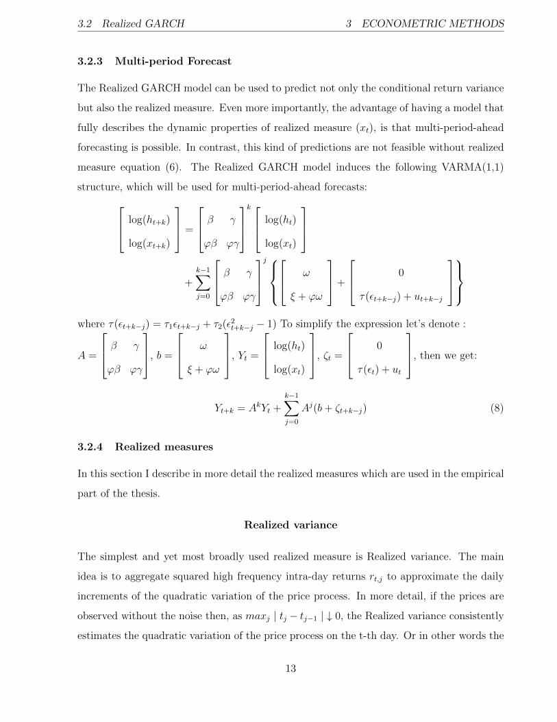
3.2.3 Multi-period Forecast
The Realized GARCH model can be used to predict not only the conditional return variance
but also the realized measure. Even more importantly, the advantage of having a model that
fully describes the dynamic properties of realized measure (xt), is that multi-period-ahead
forecasting is possible. In contrast, this kind of predictions are not feasible without realized
measure equation (6). The Realized GARCH model induces the following VARMA(1,1)
structure, which will be used for multi-period-ahead forecasts: log(ht+k)
log(xt+k)
=
β γ
ϕβ ϕγ
k log(ht)
log(xt)
+k−1∑j=0
β γ
ϕβ ϕγ
j ω
ξ + ϕω
+
0
τ(εt+k−j) + ut+k−j
where τ(εt+k−j) = τ1εt+k−j + τ2(ε2t+k−j − 1) To simplify the expression let’s denote :
A =
β γ
ϕβ ϕγ
, b =
ω
ξ + ϕω
, Yt =
log(ht)
log(xt)
, ζt =
0
τ(εt) + ut
, then we get:
Yt+k = AkYt +k−1∑j=0
Aj(b+ ζt+k−j) (8)
3.2.4 Realized measures
In this section I describe in more detail the realized measures which are used in the empirical
part of the thesis.
Realized variance
The simplest and yet most broadly used realized measure is Realized variance. The main
idea is to aggregate squared high frequency intra-day returns rt,j to approximate the daily
increments of the quadratic variation of the price process. In more detail, if the prices are
observed without the noise then, as maxj | tj − tj−1 | ↓ 0, the Realized variance consistently
estimates the quadratic variation of the price process on the t-th day. Or in other words the
13
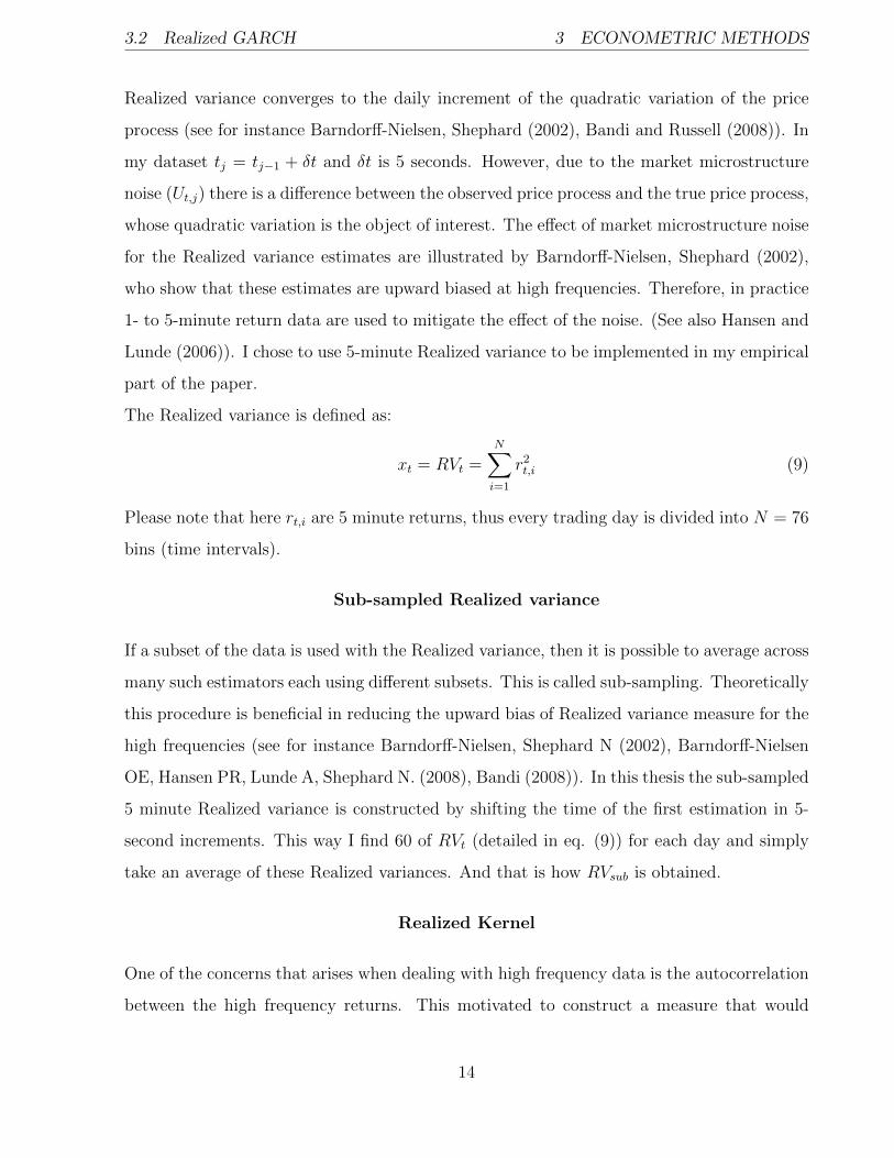
3.2 Realized GARCH 3 ECONOMETRIC METHODS
Realized variance converges to the daily increment of the quadratic variation of the price
process (see for instance Barndorff-Nielsen, Shephard (2002), Bandi and Russell (2008)). In
my dataset tj = tj−1 + δt and δt is 5 seconds. However, due to the market microstructure
noise (Ut,j) there is a difference between the observed price process and the true price process,
whose quadratic variation is the object of interest. The effect of market microstructure noise
for the Realized variance estimates are illustrated by Barndorff-Nielsen, Shephard (2002),
who show that these estimates are upward biased at high frequencies. Therefore, in practice
1- to 5-minute return data are used to mitigate the effect of the noise. (See also Hansen and
Lunde (2006)). I chose to use 5-minute Realized variance to be implemented in my empirical
part of the paper.
The Realized variance is defined as:
xt = RVt =N∑i=1
r2t,i (9)
Please note that here rt,i are 5 minute returns, thus every trading day is divided into N = 76
bins (time intervals).
Sub-sampled Realized variance
If a subset of the data is used with the Realized variance, then it is possible to average across
many such estimators each using different subsets. This is called sub-sampling. Theoretically
this procedure is beneficial in reducing the upward bias of Realized variance measure for the
high frequencies (see for instance Barndorff-Nielsen, Shephard N (2002), Barndorff-Nielsen
OE, Hansen PR, Lunde A, Shephard N. (2008), Bandi (2008)). In this thesis the sub-sampled
5 minute Realized variance is constructed by shifting the time of the first estimation in 5-
second increments. This way I find 60 of RVt (detailed in eq. (9)) for each day and simply
take an average of these Realized variances. And that is how RVsub is obtained.
Realized Kernel
One of the concerns that arises when dealing with high frequency data is the autocorrelation
between the high frequency returns. This motivated to construct a measure that would
14

3.2 Realized GARCH 3 ECONOMETRIC METHODS
account for this serial correlation. Barndorff-Nielsen OE, Hansen PR, Lunde A, Shephard
N. (2008) proposed to use Realized Kernel. Which is defined as:
xt = RKt = K(X) =H∑
h=−H
k
(h
H + 1
)γh,
where k(x) is a symmetric function, known as Parzen Kernel:
k(x) =
1− 6x2 + 6x3, 0 ≤ x ≤ 0.5
2(1− x)3, 0.5 ≤ x ≤ 1
0, x > 1
and
γh =n∑|h|+1
rt,jrt,j−|h|,
where n = bt/δtc = 4680, δt = 5 seconds and rt,j are 5 second log returns. The authors show
that as n → ∞, K(U) → 0, K(Y ) → [Y ], which implies that also we have K(X) → [X].
Recall that X is an observation of Y and U denotes the market microstructure noise.
Now I briefly show how the optimal H can be chosen. In the same paper, authors argue that
H should be find by using the formula:
H = c ξ4/5n3/5, (10)
with c = 3.5134 for the Parzen kernel k(x) detailed above and
ξ2 =ω2
RVsub
RVsub is sub-sampled Realized variance mentioned above and ω2 can be found using the
formula:
ω2 =1
q
q∑i=1
RV(i)dense
2n(i)
(11)
where RV(1)dense, ..., RV
(q)dense are Realised variances calculated using every q-th observation (ev-
ery 5th second, 10th second, 15th second and so on).
It should be noted that within the Realized Kernel framework high frequency returns can be
used (rt,j = 5 seconds). Because, in contrast to Realized variance measure, Realized Kernel
15
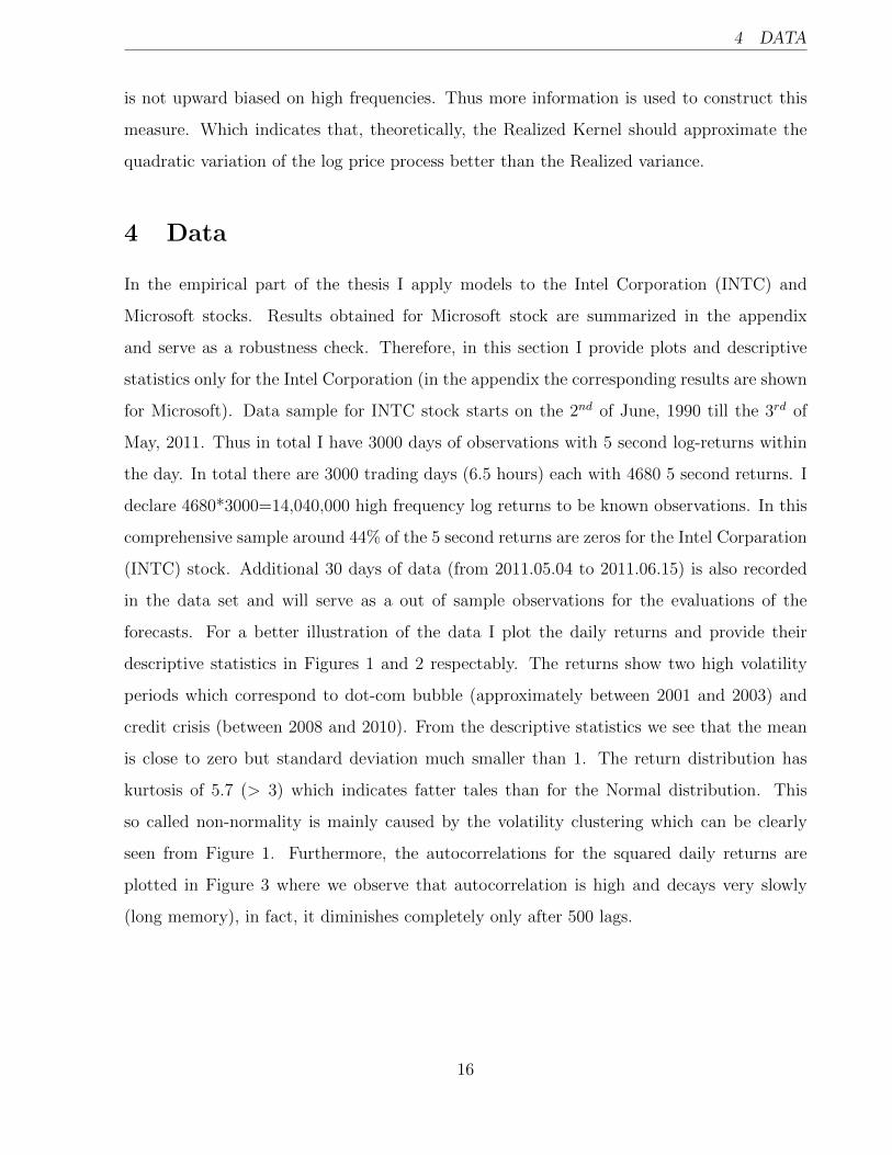
4 DATA
is not upward biased on high frequencies. Thus more information is used to construct this
measure. Which indicates that, theoretically, the Realized Kernel should approximate the
quadratic variation of the log price process better than the Realized variance.
4 Data
In the empirical part of the thesis I apply models to the Intel Corporation (INTC) and
Microsoft stocks. Results obtained for Microsoft stock are summarized in the appendix
and serve as a robustness check. Therefore, in this section I provide plots and descriptive
statistics only for the Intel Corporation (in the appendix the corresponding results are shown
for Microsoft). Data sample for INTC stock starts on the 2nd of June, 1990 till the 3rd of
May, 2011. Thus in total I have 3000 days of observations with 5 second log-returns within
the day. In total there are 3000 trading days (6.5 hours) each with 4680 5 second returns. I
declare 4680*3000=14,040,000 high frequency log returns to be known observations. In this
comprehensive sample around 44% of the 5 second returns are zeros for the Intel Corparation
(INTC) stock. Additional 30 days of data (from 2011.05.04 to 2011.06.15) is also recorded
in the data set and will serve as a out of sample observations for the evaluations of the
forecasts. For a better illustration of the data I plot the daily returns and provide their
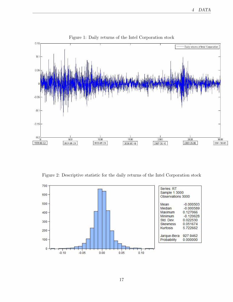
descriptive statistics in Figures 1 and 2 respectably. The returns show two high volatility
periods which correspond to dot-com bubble (approximately between 2001 and 2003) and
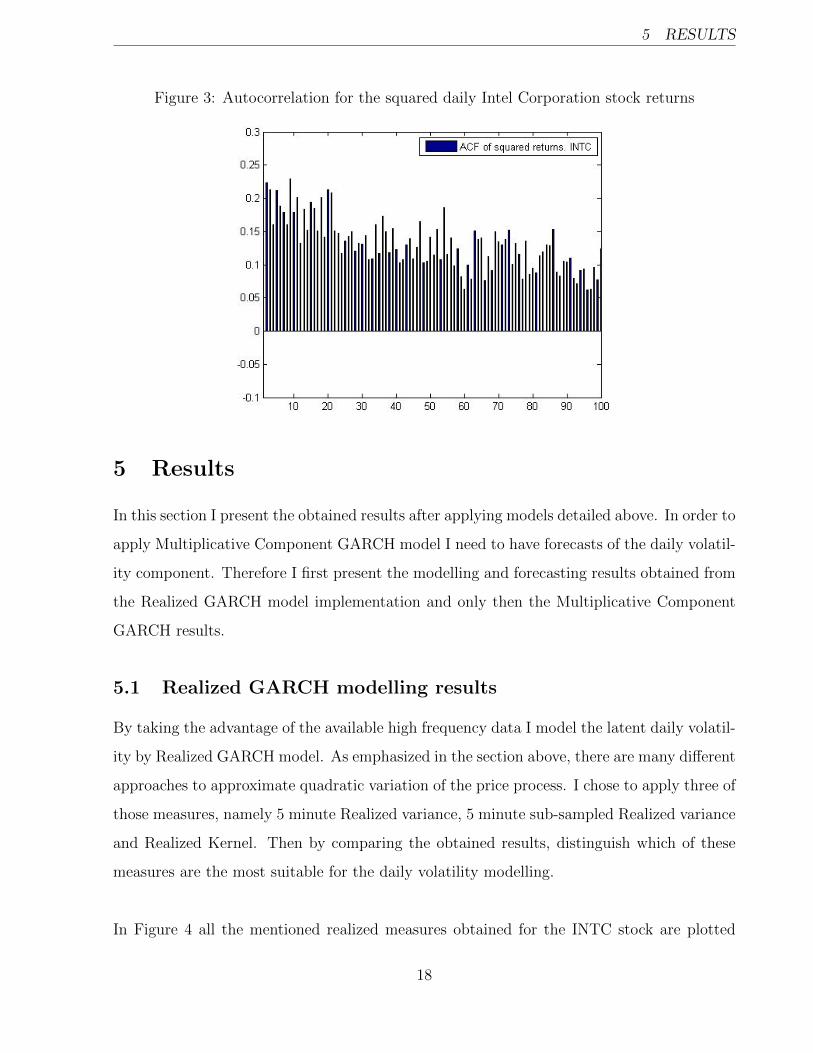
credit crisis (between 2008 and 2010). From the descriptive statistics we see that the mean
is close to zero but standard deviation much smaller than 1. The return distribution has
kurtosis of 5.7 (> 3) which indicates fatter tales than for the Normal distribution. This
so called non-normality is mainly caused by the volatility clustering which can be clearly
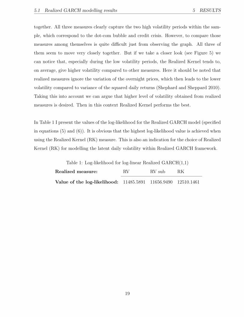
seen from Figure 1. Furthermore, the autocorrelations for the squared daily returns are
plotted in Figure 3 where we observe that autocorrelation is high and decays very slowly
(long memory), in fact, it diminishes completely only after 500 lags.
16
4 DATA
Figure 1: Daily returns of the Intel Corporation stock
Figure 2: Descriptive statistic for the daily returns of the Intel Corporation stock
17
5 RESULTS
Figure 3: Autocorrelation for the squared daily Intel Corporation stock returns
5 Results
In this section I present the obtained results after applying models detailed above. In order to
apply Multiplicative Component GARCH model I need to have forecasts of the daily volatil-
ity component. Therefore I first present the modelling and forecasting results obtained from
the Realized GARCH model implementation and only then the Multiplicative Component
GARCH results.
5.1 Realized GARCH modelling results
By taking the advantage of the available high frequency data I model the latent daily volatil-
ity by Realized GARCH model. As emphasized in the section above, there are many different
approaches to approximate quadratic variation of the price process. I chose to apply three of
those measures, namely 5 minute Realized variance, 5 minute sub-sampled Realized variance
and Realized Kernel. Then by comparing the obtained results, distinguish which of these
measures are the most suitable for the daily volatility modelling.
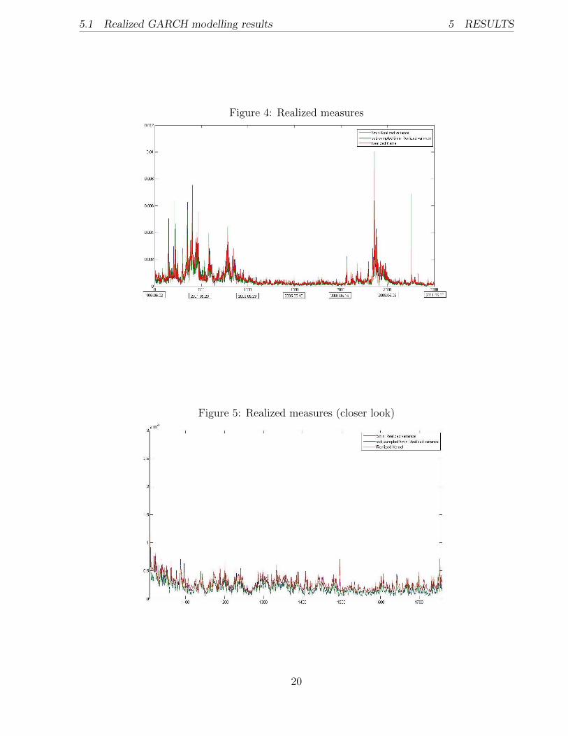
In Figure 4 all the mentioned realized measures obtained for the INTC stock are plotted
18
5.1 Realized GARCH modelling results 5 RESULTS
together. All three measures clearly capture the two high volatility periods within the sam-
ple, which correspond to the dot-com bubble and credit crisis. However, to compare those
measures among themselves is quite difficult just from observing the graph. All three of
them seem to move very closely together. But if we take a closer look (see Figure 5) we
can notice that, especially during the low volatility periods, the Realized Kernel tends to,
on average, give higher volatility compared to other measures. Here it should be noted that
realized measures ignore the variation of the overnight prices, which then leads to the lower
volatility compared to variance of the squared daily returns (Shephard and Sheppard 2010).
Taking this into account we can argue that higher level of volatility obtained from realized
measures is desired. Then in this context Realized Kernel performs the best.
In Table 1 I present the values of the log-likelihood for the Realized GARCH model (specified
in equations (5) and (6)). It is obvious that the highest log-likelihood value is achieved when
using the Realized Kernel (RK) measure. This is also an indication for the choice of Realized
Kernel (RK) for modelling the latent daily volatility within Realized GARCH framework.
Table 1: Log-likelihood for log-linear Realized GARCH(1,1)
Realized measure: RV RV sub RK
Value of the log-likelihood: 11485.5891 11656.9490 12510.1461
19
5.1 Realized GARCH modelling results 5 RESULTS
Figure 4: Realized measures
Figure 5: Realized measures (closer look)
20
5.1 Realized GARCH modelling results 5 RESULTS
Tab
le2:
Obta
ined
resu
lts
for
log-
linea
rR
ealize
dG
AR
CH
(1,1
)
Para
mete
rsSta
ndard
err
ors
Stu
dent’
st
p-v
alu
e
RV
RV
sub
RK
RV
RV
sub
RK
RV
RV
sub
RK
RV
RV
sub
RK
ω-0
.119
1-0
.149
00.
2013
0.08
240.
0933
0.12
34-1
.444
7-1
.597
31.
6306
0.14
860.
1103
0.10
31
β0.
6271
0.57
680.
5361
0.02
100.
0221
0.02
0929
.832
926
.051
425
.643
50.
0000
0.00
000.
0000
γ0.
3554
0.40
030.
5000
0.02
070.
0220
0.02
7217
.135
618
.152
318
.376
40.
0000
0.00
000.
0000
ξ-0
.080
7-0
.045
3-0
.705
60.
2151
0.21
690.
2181
-0.3
753
-0.2
091
-3.2
353
0.70
750.
8344
0.00
12
ϕ0.
9971
1.00
500.
8898
0.02
690.
0271
0.02
7337
.060
037
.056
132
.568
40.
0000
0.00
000.
0000
τ 1-0
.018
8-0
.016
7-0
.021
90.
0078
0.00
730.
0055
-2.4
163
-2.2
805
-3.9
772
0.01
570.
0226
0.00
01
τ 20.
0842
0.08
090.
0505
0.00
550.
0052
0.00
3815
.162
715
.375
913
.360
60.
0000
0.00
000.
0000
π0.
9815
0.97
900.
9810
21

5.2 Realized GARCH forecasting results 5 RESULTS
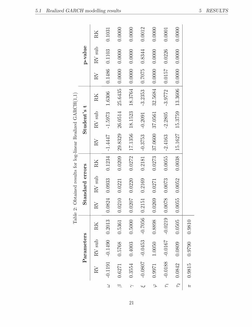
From observing results in Table 2 some important conclusions can be drawn. Almost all of
the parameters of the model are very significant with every realized measure. It can also
be clearly seen that standard (RV ) and sub-sampled 5 minute Realized variances (RVsub)
give very close results, thus sub-sampling procedure does not give empirically sufficient im-
provements in this case. However, when investigating results with Realized Kernel (RK)
few distinctions can be noticed. First, the leverage effect (captured by the parameter τ1)
becomes even more important. Also using this realised measure, the parameter ξ becomes
significant compared to other realized measures. Another important difference can be no-
ticed when RK is applied then parameter β becomes significantly smaller and γ gets bigger.
This implies that less weight is given to ht−1 and more to xt−1 which means that Realized
Kernel measure has more explanatory power for the latent daily volatility ht.
The parameter π = β + ϕγ is constrained and needs to be between (−1, 1) for the model
to be stationary (see Hansen, Huang and Shek (2011)). In fact π is the largest eigenvalue
of the matrix A in the equation (8). In Table 2 we see that this parameter has value close
to 1 no matter which realized measures is used. It indicates that autocorrelation for the
residuals of the squared returns decays slowly. Please recall that in Chapter 4 it was shown
that squared daily returns of the Intel Corporation have this long memory property. Thus
it can be concluded that Realized GARCH model captures the long memory property.
5.2 Realized GARCH forecasting results
In this part I try to distinguish which of the realized measures give the best forecasting
results within a Realized GARCH framework. As mentioned above, this model induces the
VARMA(1,1) structure for multi-period forecasts (detailed in equation (8)). The benefit of
this structure is not only the fact that we can forecast daily volatility (ht) multi periods
ahead, but also the fact that we can forecast realized measure xt as well. Therefore, in this
section the forecasts over different horizons, namely 1,2,...,30 days ahead, are found and then
compared. Moreover, the predictions for both xt and ht are obtained. In more detail, I use
a data sample of the 3000 days (from 2nd of June, 1990 till the 3rd of May, 2011) to forecast
22
5.2 Realized GARCH forecasting results 5 RESULTS
daily volatility and realized measure 1,2,...,30 days ahead.
True volatility is not observable. Thus when we want to evaluate the forecasts of the variance
we encounter a problem of choosing the right proxy for the true volatility. Often volatility
forecasts are compared to squared returns but they give a low level of information about the
variance. Another solution is to choose realized measure as a proxy for the true volatility, I
chose to use three proxies, namely 5 minute Realized variance RVout−sample, sub-sampled 5
minute Realized variance RVsub−out−sample and RKout−sample. Forecasting procedure can be
summarized like this:
(i) By applying 3 different realized measures I obtain 3 different forecasts for xt and 3 for
ht.
(ii) In order to distinguish which measure gives the best forecasts I calculate 3 out of
sample realized measures which would serve as proxies for the true volatility.
(iii) Finally comparison takes place. Forecasts obtained for the xt and ht with Realized
variance (as a measure) are compared to RVout−sample, prediction of xt and ht with
sub-sampled Realized variance are compared to RVsub−out−sample and forecasts obtained
for xt and ht with Realized Kernel are compared to RKout−sample.
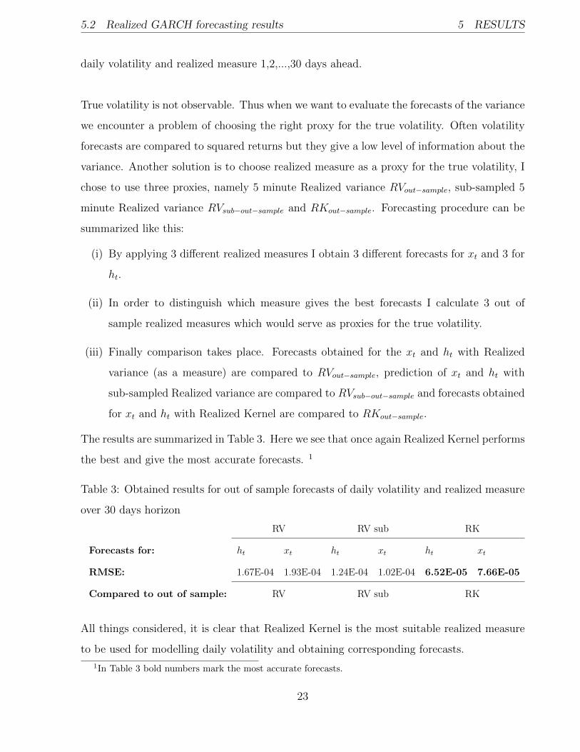
The results are summarized in Table 3. Here we see that once again Realized Kernel performs
the best and give the most accurate forecasts. 1
Table 3: Obtained results for out of sample forecasts of daily volatility and realized measure
over 30 days horizon
RV RV sub RK
Forecasts for: ht xt ht xt ht xt
RMSE: 1.67E-04 1.93E-04 1.24E-04 1.02E-04 6.52E-05 7.66E-05
Compared to out of sample: RV RV sub RK
All things considered, it is clear that Realized Kernel is the most suitable realized measure
to be used for modelling daily volatility and obtaining corresponding forecasts.
1In Table 3 bold numbers mark the most accurate forecasts.
23
5.3 Modelling results for Multiplicative Component GARCH 5 RESULTS
5.3 Modelling results for Multiplicative Component GARCH
In this section I present results obtained after applying Multiplicative Component GARCH
model (detailed in equations (1),(2) and (3)) for INTC stock. The last 30 days of observations
will be used for this model. Here ht is modelled by the Realized GARCH and as rt,i I take
15 minute returns. In total, there is 30*26=780 observations of rt,i and diurnal pattern si
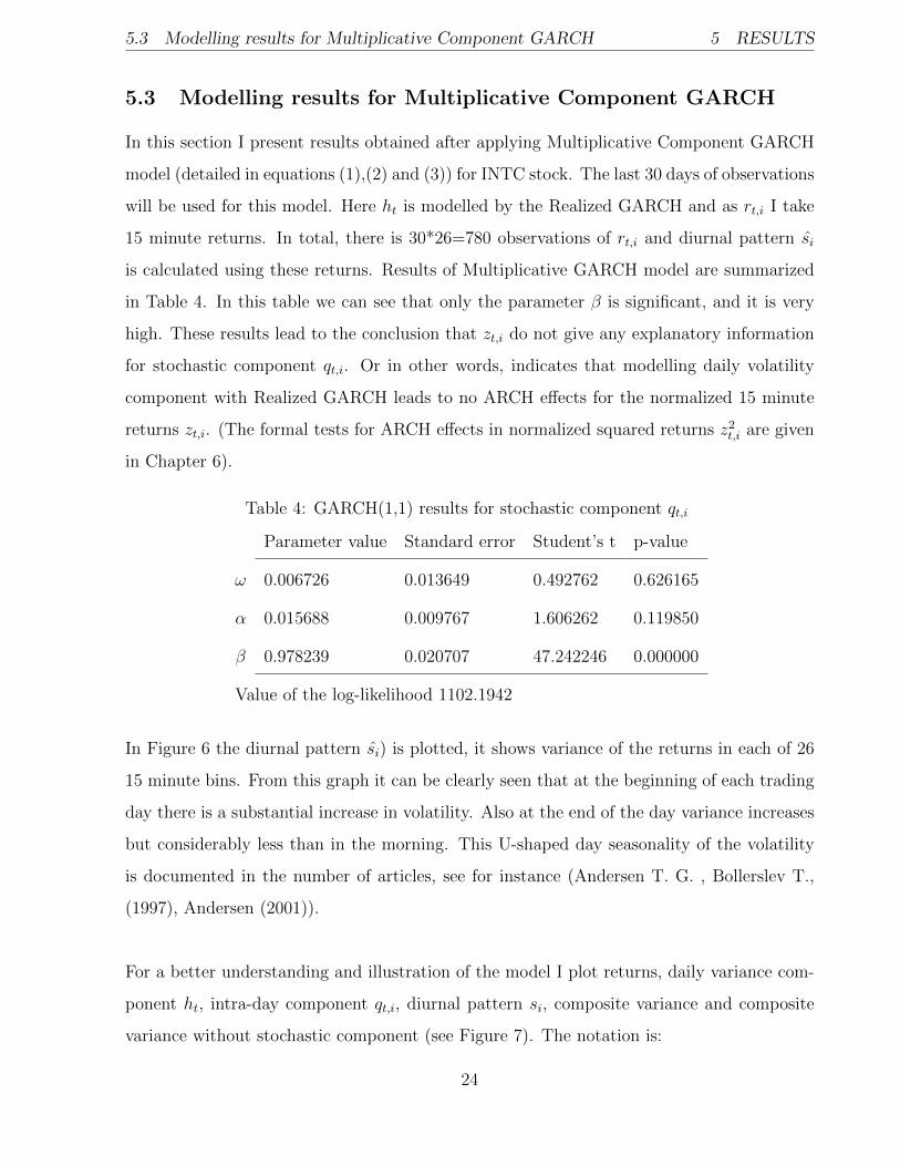
is calculated using these returns. Results of Multiplicative GARCH model are summarized
in Table 4. In this table we can see that only the parameter β is significant, and it is very
high. These results lead to the conclusion that zt,i do not give any explanatory information
for stochastic component qt,i. Or in other words, indicates that modelling daily volatility
component with Realized GARCH leads to no ARCH effects for the normalized 15 minute
returns zt,i. (The formal tests for ARCH effects in normalized squared returns z2t,i are given
in Chapter 6).
Table 4: GARCH(1,1) results for stochastic component qt,i
Parameter value Standard error Student’s t p-value
ω 0.006726 0.013649 0.492762 0.626165
α 0.015688 0.009767 1.606262 0.119850
β 0.978239 0.020707 47.242246 0.000000
Value of the log-likelihood 1102.1942
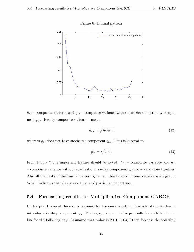
In Figure 6 the diurnal pattern si) is plotted, it shows variance of the returns in each of 26
15 minute bins. From this graph it can be clearly seen that at the beginning of each trading
day there is a substantial increase in volatility. Also at the end of the day variance increases
but considerably less than in the morning. This U-shaped day seasonality of the volatility
is documented in the number of articles, see for instance (Andersen T. G. , Bollerslev T.,
(1997), Andersen (2001)).
For a better understanding and illustration of the model I plot returns, daily variance com-
ponent ht, intra-day component qt,i, diurnal pattern si, composite variance and composite
variance without stochastic component (see Figure 7). The notation is:
24
5.4 Forecasting results for Multiplicative Component GARCH 5 RESULTS
Figure 6: Diurnal pattern
ht,i – composite variance and gt,i – composite variance without stochastic intra-day compo-
nent qt,i. Here by composite variance I mean:
ht,i =√htsiqt,i (12)
whereas gt,i does not have stochastic component qt,i. Thus it is equal to:
gt,i =√htsi. (13)
From Figure 7 one important feature should be noted: ht,i – composite variance and gt,i
– composite variance without stochastic intra-day component qt,i move very close together.
Also all the peaks of the diurnal pattern si remain clearly vivid in composite variance graph.
Which indicates that day seasonality is of particular importance.
5.4 Forecasting results for Multiplicative Component GARCH
In this part I present the results obtained for the one step ahead forecasts of the stochastic
intra-day volatility component qt,i. That is, qt,i is predicted sequentially for each 15 minute
bin for the following day. Assuming that today is 2011.05.03, I then forecast the volatility
25

5.4 Forecasting results for Multiplicative Component GARCH 5 RESULTS
Figure 7: Volatility components
for each 15 minute time interval for the next day, that is 2011.05.04. The procedure can be
summarized as follows:
(i) I take the daily variance component ht modelled by Realized GARCH.
(ii) Then si is calculated as detailed above.
(iii) Having this information I model the stochastic intra-day volatility component qt,i by
GARCH(1,1) and forecast it one period ahead qt+1,1. This way I obtain the prediction
for the first 15 minute bin of 2011.05.04.
(iv) Let’s assume that the first 15 minutes of the day 2011.05.04 have passed, that is rt+1,1
is now known. Using this additional information and the forecast of the daily volatility
component ht+1 (see equation (8)), now qt+1,2 can be predicted.
This procedure is then repeated till qt+1,i, ∀ i = 1, ..., N is found. Here N indicates number
of bins in one trading day and is equal to 26 because in total there are 26 bins of 15 minute
time intervals in one trading day.
26
5.4 Forecasting results for Multiplicative Component GARCH 5 RESULTS
When we want to evaluate the forecasts of the volatility we encounter a problem of choosing
the right proxy of the true volatility. Here a true volatility for every bin in each day is de-
noted as σ2t,i. And to evaluate this σ2
t,i, 3 volatility proxies are employed, namely r2t,i, RVsub t,i
and RKt,i. In more detail, r2t,i are squared 15 minute returns, RVsub t,i is a sub-sampled 1
minute Realized variance for every 15 minute time interval and RKt,i – a 15 minute Realized
Kernel (detailed explanation of the calculation procedure of this measure can be found in
the appendix).
I choose to compare ht,i-composite intra-day variance and gt,i-composite intra-day variance
without stochastic component (detailed in 12 and 13) to the true volatility proxies. This
way I can determine whether the inclusion of the predicted stochastic intra-day component
qt,i makes the forecasts more accurate or not. For this purpose Root mean squared error
(RMSE) is implemented. It is calculated as follows:
(i) RMSE =√
1N
∑Ni=1
(σ2t,i − ht,i
)2
(ii) RMSE =√
1N
∑Ni=1
(σ2t,i − gt,i
)2
where σ2t,i is one of the three mentioned volatility proxies.
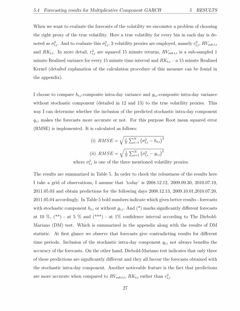
The results are summarized in Table 5. In order to check the robustness of the results here
I take a grid of observations, I assume that ’today’ is 2008.12.12, 2009.09.30, 2010.07.19,
2011.05.03 and obtain predictions for the following days 2008.12.13, 2009.10.01,2010.07.20,
2011.05.04 accordingly. In Table 5 bold numbers indicate which gives better results - forecasts
with stochastic component ht,i or without gt,i. And (*) marks significantly different forecasts
at 10 %, (**) - at 5 % and (***) - at 1% confidence interval according to The Diebold-
Mariano (DM) test. Which is summarized in the appendix along with the results of DM
statistic. At first glance we observe that forecasts give contradicting results for different
time periods. Inclusion of the stochastic intra-day component qt,i not always benefits the
accuracy of the forecasts. On the other hand, Diebold-Mariano test indicates that only three
of these predictions are significantly different and they all favour the forecasts obtained with
the stochastic intra-day component. Another noticeable feature is the fact that predictions
are more accurate when compared to RVsub.t,i, RKt,i rather than r2t,i.
27
5.4 Forecasting results for Multiplicative Component GARCH 5 RESULTS
Table 5: RMSE comparison for composite variance
RMSE
Date: 2008.12.12 2009.09.30 2010.07.19 2011.05.03
Forecasts of: ht,i gt,i ht,i gt,i ht,i gt,i ht,i gt,i
Compared to proxies:
r2t,i 2.148E-09*** 2.377E-09 1.55E-10 1.83E-10 8.3E-11*** 8.9E-11 1.96E-10 1.52E-10
RVsub.t,i 1.103E-09 1.084E-09 6.4E-11 8.1E-11 1.5E-11 1.6E-11 1E-10 5.2E-11
RKt,i 8.47E-10 7.98E-10 7.6E-11*** 1.18E-10 1.2E-11 1.2E-11 5E-11 4.3E-11
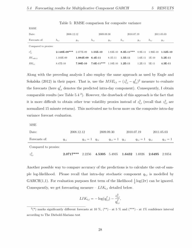
Along with the preceding analysis I also employ the same approach as used by Engle and
Sokalska (2012) in their paper. That is, use the MSEt,i = (z2t,i − q
ft,i)
2 measure to evaluate
the forecasts (here qft,i denotes the predicted intra-day component). Consequently, I obtain
comparable results (see Table 5.4 2). However, the drawback of this approach is the fact that
it is more difficult to obtain other true volatility proxies instead of z2t,i (recall that z2
t,i are
normalized 15 minute returns). This motivated me to focus more on the composite intra-day
variance forecast evaluation.
MSE
Date: 2008.12.12 2009.09.30 2010.07.19 2011.05.03
Forecasts of: qt,i qt,i = 1 qt,i qt,i = 1 qt,i qt,i = 1 qt,i qt,i = 1
Compared to proxies:
z2t,i 2.0717*** 2.2256 4.5305 5.4935 1.6432 1.6926 2.6495 2.9354
Another possible way to compare accuracy of the predictions is to calculate the out-of sam-
ple log-likelihood. Please recall that intra-day stochastic component qt,i is modelled by
GARCH(1,1). For evaluation purposes first term of the likelihood 12
log(2π) can be ignored.
Consequently, we get forecasting measure – LIKt,i detailed below.
LIKt,i = − log(qft,i)−z2t,i
qft,i,
2(*) marks significantly different forecasts at 10 %, (**) - at 5 % and (***) - at 1% confidence interval
according to The Diebold-Mariano test
28
5.4 Forecasting results for Multiplicative Component GARCH 5 RESULTS
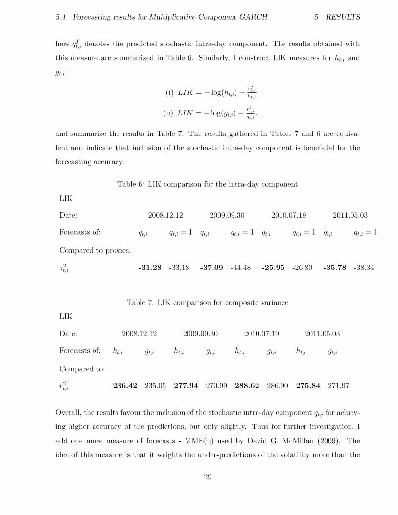
here qft,i denotes the predicted stochastic intra-day component. The results obtained with
this measure are summarized in Table 6. Similarly, I construct LIK measures for ht,i and
gt,i:
(i) LIK = − log(ht,i)−r2t,iht,i
(ii) LIK = − log(gt,i)−r2t,igt,i
.
and summarize the results in Table 7. The results gathered in Tables 7 and 6 are equiva-
lent and indicate that inclusion of the stochastic intra-day component is beneficial for the
forecasting accuracy.
Table 6: LIK comparison for the intra-day component
LIK
Date: 2008.12.12 2009.09.30 2010.07.19 2011.05.03
Forecasts of: qt,i qt,i = 1 qt,i qt,i = 1 qt,i qt,i = 1 qt,i qt,i = 1
Compared to proxies:
z2t,i -31.28 -33.18 -37.09 -44.48 -25.95 -26.80 -35.78 -38.34
Table 7: LIK comparison for composite variance
LIK
Date: 2008.12.12 2009.09.30 2010.07.19 2011.05.03
Forecasts of: ht,i gt,i ht,i gt,i ht,i gt,i ht,i gt,i
Compared to:
r2t,i 236.42 235.05 277.94 270.99 288.62 286.90 275.84 271.97
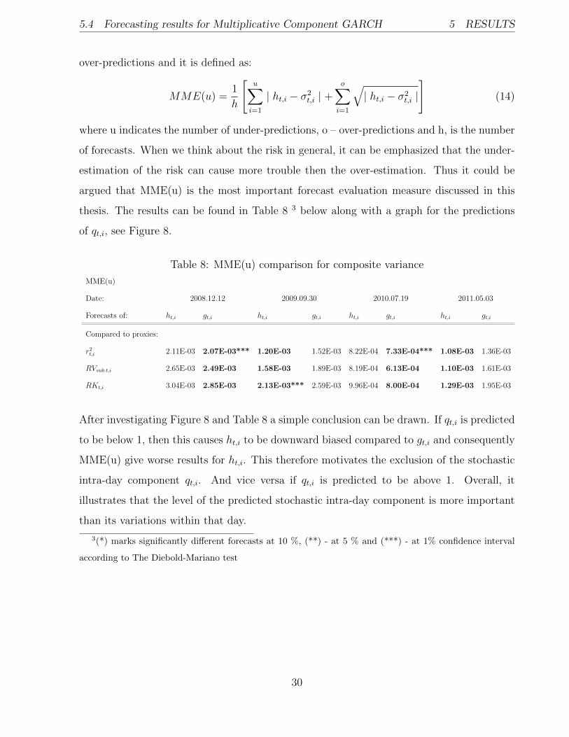
Overall, the results favour the inclusion of the stochastic intra-day component qt,i for achiev-
ing higher accuracy of the predictions, but only slightly. Thus for further investigation, I
add one more measure of forecasts - MME(u) used by David G. McMillan (2009). The
idea of this measure is that it weights the under-predictions of the volatility more than the
29
5.4 Forecasting results for Multiplicative Component GARCH 5 RESULTS
over-predictions and it is defined as:
MME(u) =1
h
[u∑
i=1
| ht,i − σ2t,i | +
o∑i=1
√| ht,i − σ2
t,i |
](14)
where u indicates the number of under-predictions, o – over-predictions and h, is the number
of forecasts. When we think about the risk in general, it can be emphasized that the under-
estimation of the risk can cause more trouble then the over-estimation. Thus it could be
argued that MME(u) is the most important forecast evaluation measure discussed in this
thesis. The results can be found in Table 8 3 below along with a graph for the predictions
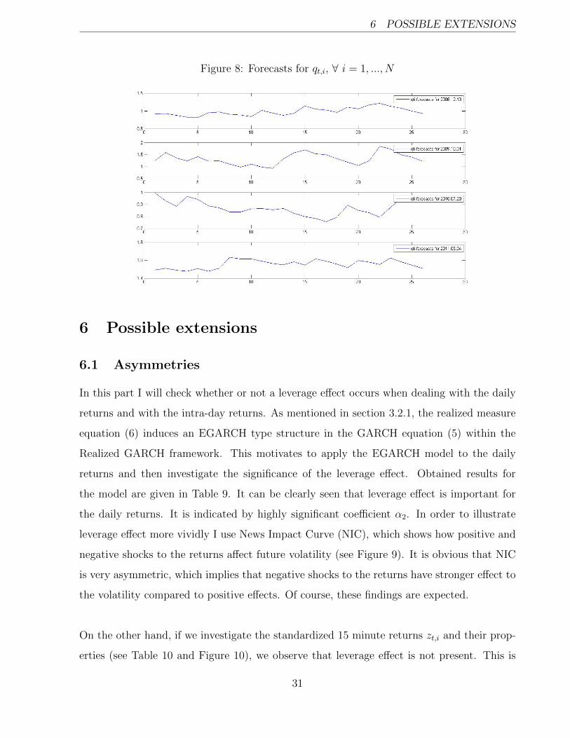
of qt,i, see Figure 8.
Table 8: MME(u) comparison for composite variance
MME(u)
Date: 2008.12.12 2009.09.30 2010.07.19 2011.05.03
Forecasts of: ht,i gt,i ht,i gt,i ht,i gt,i ht,i gt,i
Compared to proxies:
r2t,i 2.11E-03 2.07E-03*** 1.20E-03 1.52E-03 8.22E-04 7.33E-04*** 1.08E-03 1.36E-03
RVsub.t,i 2.65E-03 2.49E-03 1.58E-03 1.89E-03 8.19E-04 6.13E-04 1.10E-03 1.61E-03
RKt,i 3.04E-03 2.85E-03 2.13E-03*** 2.59E-03 9.96E-04 8.00E-04 1.29E-03 1.95E-03
After investigating Figure 8 and Table 8 a simple conclusion can be drawn. If qt,i is predicted
to be below 1, then this causes ht,i to be downward biased compared to gt,i and consequently
MME(u) give worse results for ht,i. This therefore motivates the exclusion of the stochastic
intra-day component qt,i. And vice versa if qt,i is predicted to be above 1. Overall, it
illustrates that the level of the predicted stochastic intra-day component is more important
than its variations within that day.
3(*) marks significantly different forecasts at 10 %, (**) - at 5 % and (***) - at 1% confidence interval
according to The Diebold-Mariano test
30
6 POSSIBLE EXTENSIONS
Figure 8: Forecasts for qt,i, ∀ i = 1, ..., N
6 Possible extensions
6.1 Asymmetries
In this part I will check whether or not a leverage effect occurs when dealing with the daily
returns and with the intra-day returns. As mentioned in section 3.2.1, the realized measure
equation (6) induces an EGARCH type structure in the GARCH equation (5) within the
Realized GARCH framework. This motivates to apply the EGARCH model to the daily
returns and then investigate the significance of the leverage effect. Obtained results for
the model are given in Table 9. It can be clearly seen that leverage effect is important for
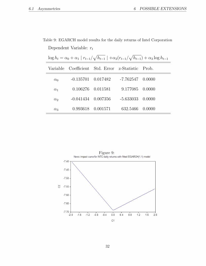
the daily returns. It is indicated by highly significant coefficient α2. In order to illustrate
leverage effect more vividly I use News Impact Curve (NIC), which shows how positive and
negative shocks to the returns affect future volatility (see Figure 9). It is obvious that NIC
is very asymmetric, which implies that negative shocks to the returns have stronger effect to
the volatility compared to positive effects. Of course, these findings are expected.
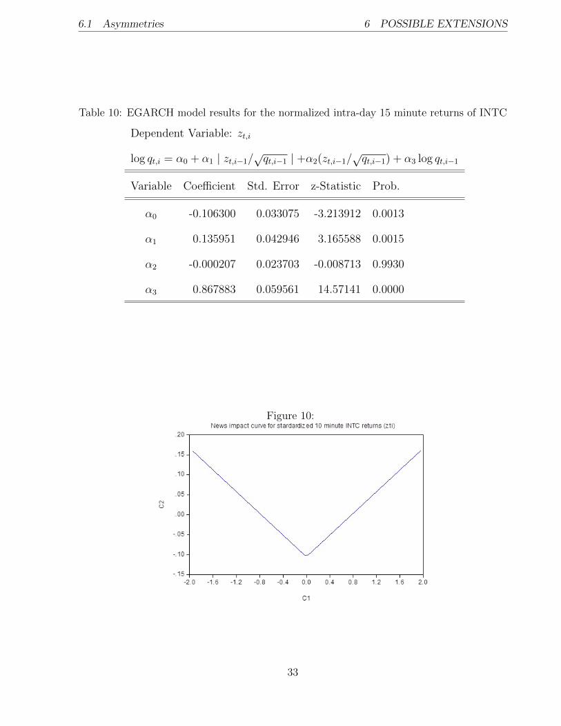
On the other hand, if we investigate the standardized 15 minute returns zt,i and their prop-
erties (see Table 10 and Figure 10), we observe that leverage effect is not present. This is
31
6.1 Asymmetries 6 POSSIBLE EXTENSIONS
Table 9: EGARCH model results for the daily returns of Intel Corporation
Dependent Variable: rt
log ht = α0 + α1 | rt−1/√ht−1 | +α2(rt−1/
√ht−1) + α3 log ht−1
Variable Coefficient Std. Error z-Statistic Prob.
α0 -0.135701 0.017482 -7.762547 0.0000
α1 0.106276 0.011581 9.177085 0.0000
α2 -0.041434 0.007356 -5.633033 0.0000
α3 0.993618 0.001571 632.5466 0.0000
Figure 9:
32
6.1 Asymmetries 6 POSSIBLE EXTENSIONS
Table 10: EGARCH model results for the normalized intra-day 15 minute returns of INTC
Dependent Variable: zt,i
log qt,i = α0 + α1 | zt,i−1/√qt,i−1 | +α2(zt,i−1/
√qt,i−1) + α3 log qt,i−1
Variable Coefficient Std. Error z-Statistic Prob.
α0 -0.106300 0.033075 -3.213912 0.0013
α1 0.135951 0.042946 3.165588 0.0015
α2 -0.000207 0.023703 -0.008713 0.9930
α3 0.867883 0.059561 14.57141 0.0000
Figure 10:
33
6.2 Long memory 6 POSSIBLE EXTENSIONS
indicated by the insignificant coefficient α2 and a symmetric News impact curve.
All things considered, it can be concluded that for the leverage effect to have a significant
importance longer period of time needs to be considered. Or in other words, leverage effect
takes longer to occur. Which is the reason why in this thesis leverage effect is accounted for
in the daily volatility modelling but not on the intra-day basis (where stochastic component
is modelled by a simple GARCH(1,1)).
6.2 Long memory
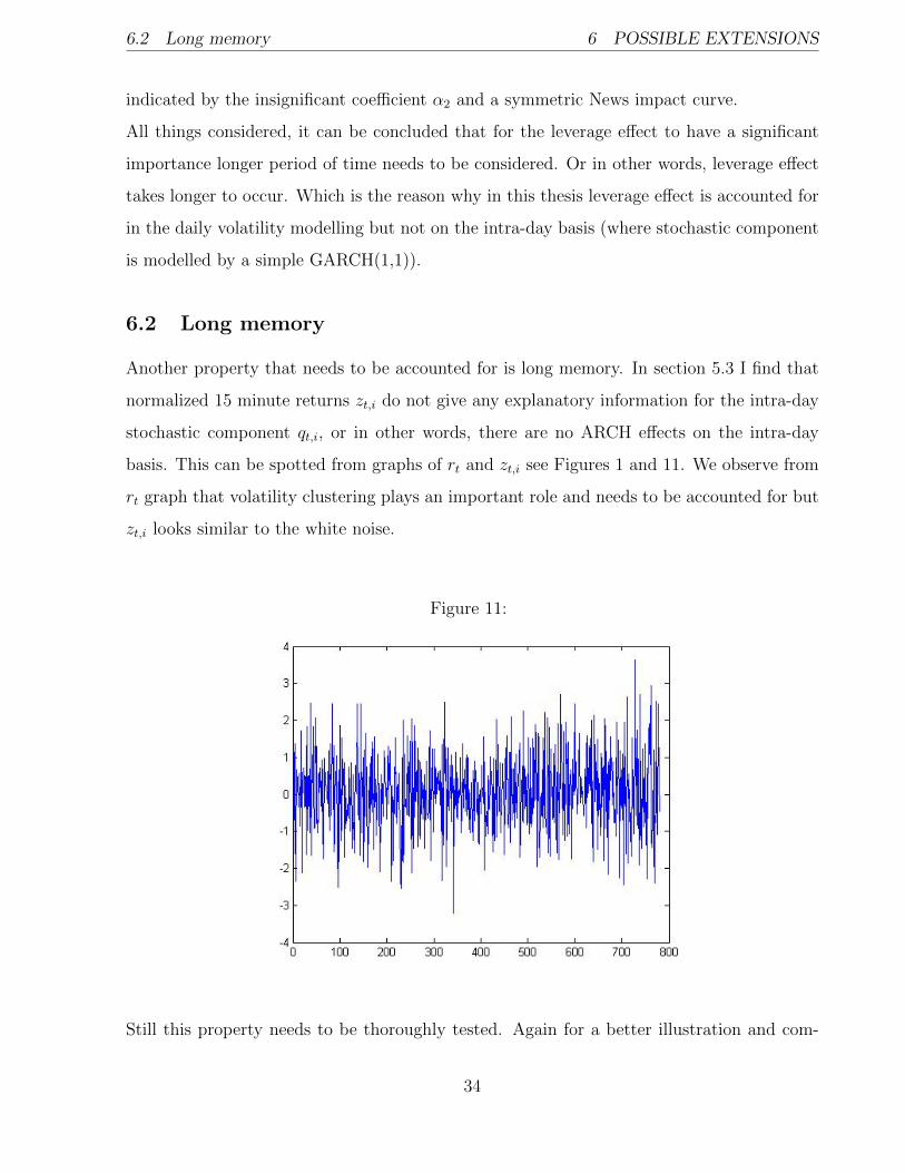
Another property that needs to be accounted for is long memory. In section 5.3 I find that
normalized 15 minute returns zt,i do not give any explanatory information for the intra-day
stochastic component qt,i, or in other words, there are no ARCH effects on the intra-day
basis. This can be spotted from graphs of rt and zt,i see Figures 1 and 11. We observe from
rt graph that volatility clustering plays an important role and needs to be accounted for but
zt,i looks similar to the white noise.
Figure 11:
Still this property needs to be thoroughly tested. Again for a better illustration and com-
34
6.2 Long memory 6 POSSIBLE EXTENSIONS
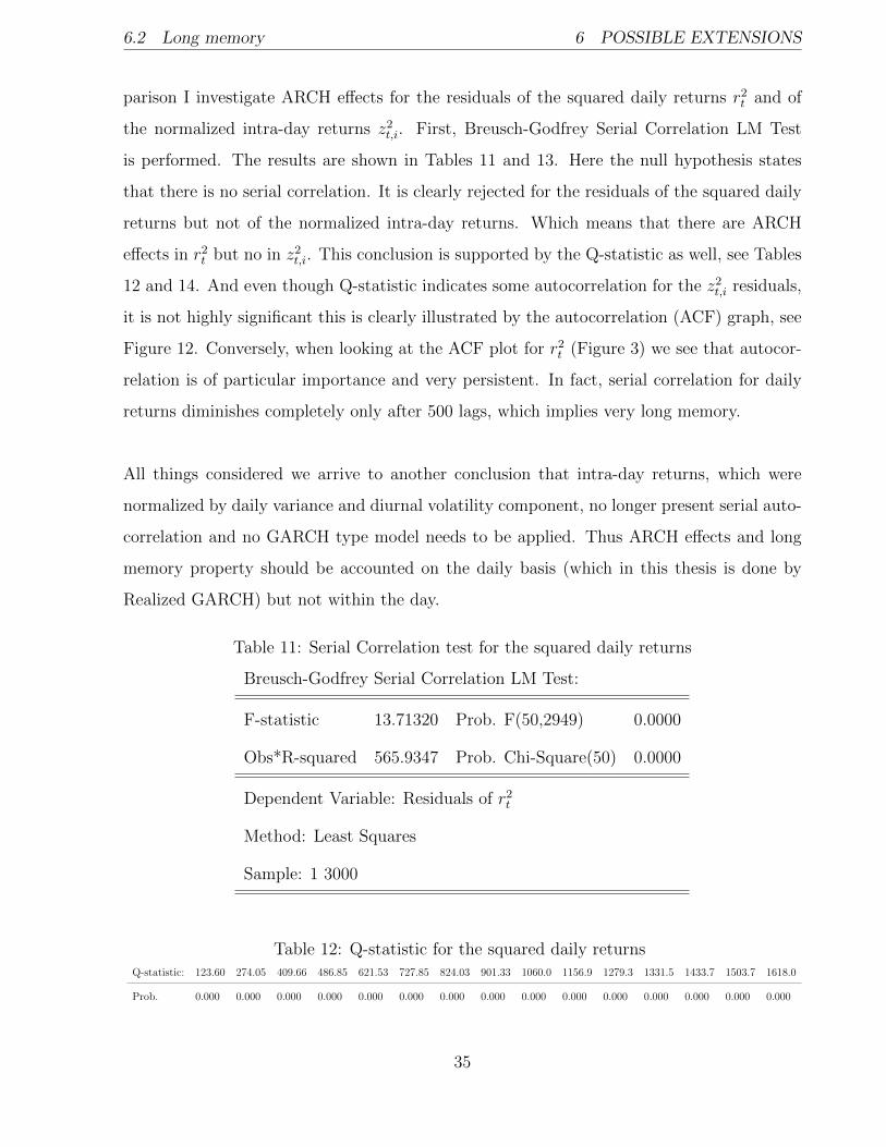
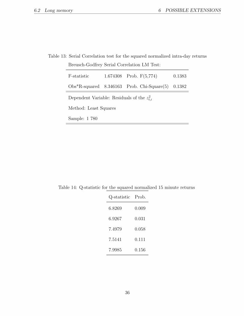
parison I investigate ARCH effects for the residuals of the squared daily returns r2t and of
the normalized intra-day returns z2t,i. First, Breusch-Godfrey Serial Correlation LM Test
is performed. The results are shown in Tables 11 and 13. Here the null hypothesis states
that there is no serial correlation. It is clearly rejected for the residuals of the squared daily
returns but not of the normalized intra-day returns. Which means that there are ARCH
effects in r2t but no in z2
t,i. This conclusion is supported by the Q-statistic as well, see Tables
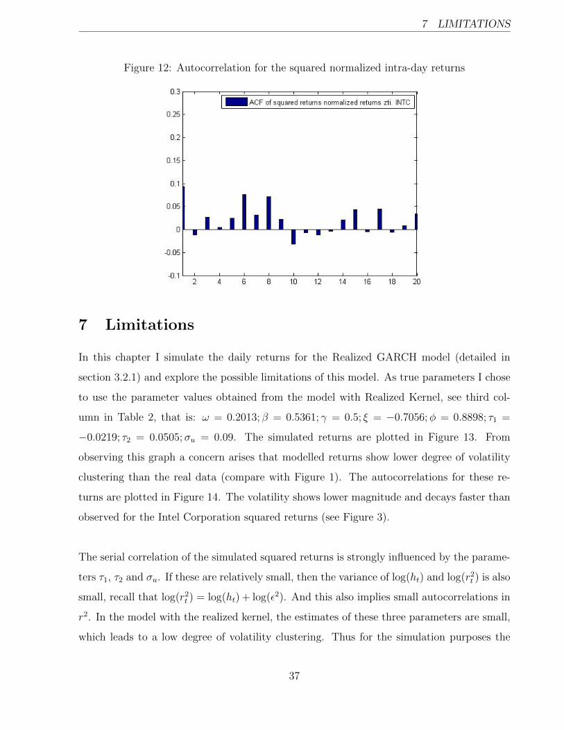
12 and 14. And even though Q-statistic indicates some autocorrelation for the z2t,i residuals,
it is not highly significant this is clearly illustrated by the autocorrelation (ACF) graph, see
Figure 12. Conversely, when looking at the ACF plot for r2t (Figure 3) we see that autocor-
relation is of particular importance and very persistent. In fact, serial correlation for daily
returns diminishes completely only after 500 lags, which implies very long memory.
All things considered we arrive to another conclusion that intra-day returns, which were
normalized by daily variance and diurnal volatility component, no longer present serial auto-
correlation and no GARCH type model needs to be applied. Thus ARCH effects and long
memory property should be accounted on the daily basis (which in this thesis is done by
Realized GARCH) but not within the day.
Table 11: Serial Correlation test for the squared daily returns
Breusch-Godfrey Serial Correlation LM Test:
F-statistic 13.71320 Prob. F(50,2949) 0.0000
Obs*R-squared 565.9347 Prob. Chi-Square(50) 0.0000
Dependent Variable: Residuals of r2t
Method: Least Squares
Sample: 1 3000
Table 12: Q-statistic for the squared daily returnsQ-statistic: 123.60 274.05 409.66 486.85 621.53 727.85 824.03 901.33 1060.0 1156.9 1279.3 1331.5 1433.7 1503.7 1618.0
Prob. 0.000 0.000 0.000 0.000 0.000 0.000 0.000 0.000 0.000 0.000 0.000 0.000 0.000 0.000 0.000
35
6.2 Long memory 6 POSSIBLE EXTENSIONS
Table 13: Serial Correlation test for the squared normalized intra-day returns
Breusch-Godfrey Serial Correlation LM Test:
F-statistic 1.674308 Prob. F(5,774) 0.1383
Obs*R-squared 8.346163 Prob. Chi-Square(5) 0.1382
Dependent Variable: Residuals of the z2t,i
Method: Least Squares
Sample: 1 780
Table 14: Q-statistic for the squared normalized 15 minute returns
Q-statistic Prob.
6.8269 0.009
6.9267 0.031
7.4979 0.058
7.5141 0.111
7.9985 0.156
36
7 LIMITATIONS
Figure 12: Autocorrelation for the squared normalized intra-day returns
7 Limitations
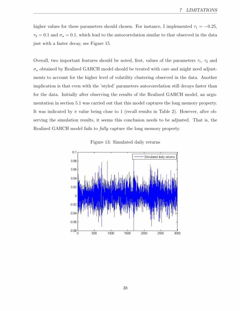
In this chapter I simulate the daily returns for the Realized GARCH model (detailed in
section 3.2.1) and explore the possible limitations of this model. As true parameters I chose
to use the parameter values obtained from the model with Realized Kernel, see third col-
umn in Table 2, that is: ω = 0.2013; β = 0.5361; γ = 0.5; ξ = −0.7056;φ = 0.8898; τ1 =
−0.0219; τ2 = 0.0505;σu = 0.09. The simulated returns are plotted in Figure 13. From
observing this graph a concern arises that modelled returns show lower degree of volatility
clustering than the real data (compare with Figure 1). The autocorrelations for these re-
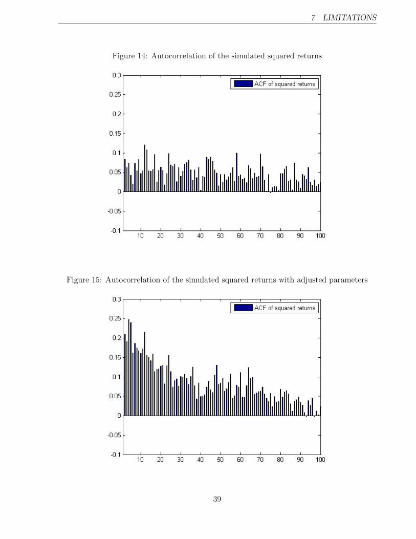
turns are plotted in Figure 14. The volatility shows lower magnitude and decays faster than
observed for the Intel Corporation squared returns (see Figure 3).
The serial correlation of the simulated squared returns is strongly influenced by the parame-
ters τ1, τ2 and σu. If these are relatively small, then the variance of log(ht) and log(r2t ) is also
small, recall that log(r2t ) = log(ht) + log(ε2). And this also implies small autocorrelations in
r2. In the model with the realized kernel, the estimates of these three parameters are small,
which leads to a low degree of volatility clustering. Thus for the simulation purposes the
37
7 LIMITATIONS
higher values for these parameters should chosen. For instance, I implemented τ1 = −0.25,
τ2 = 0.1 and σu = 0.1, which lead to the autocorrelation similar to that observed in the data
just with a faster decay, see Figure 15.
Overall, two important features should be noted, first, values of the parameters τ1, τ2 and
σu obtained by Realized GARCH model should be treated with care and might need adjust-
ments to account for the higher level of volatility clustering observed in the data. Another
implication is that even with the ’styled’ parameters autocorrelation still decays faster than
for the data. Initially after observing the results of the Realized GARCH model, an argu-
mentation in section 5.1 was carried out that this model captures the long memory property.
It was indicated by π value being close to 1 (recall results in Table 2). However, after ob-
serving the simulation results, it seems this conclusion needs to be adjusted. That is, the
Realized GARCH model fails to fully capture the long memory property.
Figure 13: Simulated daily returns
38
7 LIMITATIONS
Figure 14: Autocorrelation of the simulated squared returns
Figure 15: Autocorrelation of the simulated squared returns with adjusted parameters
39
8 CONCLUSIONS
8 Conclusions
First of all, I would like to draw some important conclusions regarding Realized GARCH
model. It was extensively shown that within the framework of this model appliance of Real-
ized Kernel provides the most accurate results. It was shown to be so in terms of modelling
and forecasting. This motivates that quadratic variation of the underlying true price process
should be modelled by the Realized Kernel rather than the Realized variance. However,
even then the simulation of the daily returns indicated that Realized GARCH does not fully
capture the volatility clustering and its persistence that is observed in the data.
In terms of Multiplicative Component GARCH model, the importance of diurnal pattern is
emphasized. In fact, the clear shape of this pattern obtained here coincides with the results
in many papers regarding Intra-day volatility. The majority of the forecasting measures
favour the inclusion of the stochastic intra-day volatility component but its significance
is still doubtful. Forecasting results evaluated by various measures give close results which
sometime are contradicting. Therefore additional forecasting measure was added – MME(u),
which penalizes under-predictions more than over-predictions. This measure indicated that a
stochastic intra-day component should be included in the model, if it is predicted to be above
1. Thus importance lies within the predicted level of the stochastic component rather than
its variations within the day. In-depth analysis of the intra-day returns (normalized by daily
variance component forecasts formed with Realized GARCH model and by deterministic
diurnal pattern) shows that no GARCH type model is needed on the intra-day basis. In
more detail, no asymmetries and, in fact, no significant serial correlation is observed for the
standardized squared 15 minute returns. Consequently, we can argue that modelling the
daily and distinguishing the diurnal volatility components is of substantial importance in
order to forecast the intra-day variance combined with accurate predictions of the level of
the stochastic intra-day component.
40
REFERENCES REFERENCES
References
[1] Andersen T.G., Bollerslev T. 1997. Intraday periodicity and volatility persistence in
financial markets. Journal of Empirical Finance 4 (1997) 115-158.
[2] Andersen T.G., Bollerslev T. 1998. Answering the skeptics: yes, standard volatility
models do provide accurateforecasts. International Economic Review 39(4): 885–905.
[3] Andersen T.G., Bollerslev T., Ashish D. 2001. Variance-ratio Statistics and High-
frequency Data: Testing for Changes in Intraday Volatility Patterns. The Journal of
Finance, 2001, Vol.56(1), pp.305-327
[4] Andersen T.G., Bollerslev T., Diebold FX, Labys P. 2001. The distribution of exchange
rate volatility. Journal of the American Statistical Association 96(453): 42–55 (correc-
tion published 2003, Vol. 98, p. 501).
[5] Andersen T.G., Bollerslev T., Diebold FX, Labys P. 2003. Modeling and forecasting
realized volatility. Econometrica 71(2): 579–625.
[6] Bandi F.M., Russell J.R. 2008. Microstructure Noise, Realized Variance, and Optimal
Sampling. Review of Economic Studies 75, 339–369.
[7] Barndorff-Nielsen O.E., Shephard N. 2002. Econometric analysis of realised volatility
and its use in estimating stochastic volatility models. Journal of the Royal Statistical
Society B 64: 253–280.
[8] Barndorff-Nielsen O.E., Shephard N. 2004. Power and bipower variation with stochastic
volatility and jumps(with discussion). Journal of Financial Econometrics 2: 1–48.
[9] Barndorff-Nielsen O.E., Hansen P.R., Lunde A., Shephard N. 2008. Designing realised
kernels to measure the ex-post variation of equity prices in the presence of noise. Econo-
metrica 76: 1481–536.
[10] Barndorff-Nielsen O.E., Hansen P.R., Lunde A., Shephard N. 2009a. Realised kernels
in practice: trades and quotes. Econometrics Journal 12: 1–33.
41
REFERENCES REFERENCES
[11] Engle R.F. 2002. New frontiers of ARCH models. Journal of Applied Econometrics 17:
425–446.
[12] Engle R.F., Gallo G. 2006. A multiple indicators model for volatility using intra-daily
data. Journal of Econometrics 131: 3–27.
[13] Engle R.F., Sokalska M. E. 2012. Forecasting intraday volatility in the US equity market.
Multiplicative Component GARCH. JournalofFinancialEconom etrics, 2012, Vol. 10,
No. 1, 54–83.
[14] Etheridge A. 2002. A Course in Financial Calculus.
[15] Ghose D., and Kroner. K. 1996. Components of Volatility in Foreign Exchange Markets:
An Empirical Analysis of High Frequency Data. Unpublished manuscript, Department
of Economics, University of Arizona.
[16] Giot P., 2005. Market Risk Models for Intraday Data. European Journal of Finance 11:
309–324.
[17] Hansen P.R., Lunde A. 2006. Consistent Ranking of Volatility Models. Journal of Econo-
metrics 131: 97–121.
[18] Hansen P.R., Huang Z., Shek H.H. 2011. Realized GARCH: A joint model for returns
and realized measures of volatility. Journal of Applied Econometrics 27: 877–906.
[19] Mcmillan D.G., Garcia R.Q. 2009. Intra-day volatility forecasts. Applied Financial
Economics,19,611-623.
[20] Shephard N., Sheppard K. 2010. Realising the future: forecasting with high frequency
based volatility (HEAVY) models. Journal of Applied Econometrics 25: 197–231.
42

A APPENDIX
A Appendix
A.1 15 minute Realized Kernel calculation
In order to calculate 15 minute RKt,i the same procedure as in section 3.2.4 is employed. Just
here to find the optimal H for every 15 minute bin I calculate 1 minute sub-sampled Realized
Variance. And use every 5, 10,..., 150 seconds returns in order to findRV(1)dense, RV
(2)dense..., RV
(q)dense
and then consequently ω and H for the every 15 minute time interval is obtained.
A.2 Diebold-Mariano test for Comparing Predictive Accuracy
Let yt denote the series to be predicted, also assume that we have two obtained forecasts y1t ,
y2t . Then ε1t = yt − y1
t and ε2t = yt − y2t can be constructed. The interest lies in evaluating
whether or not the accuracy of the forecasts differ. The accuracy of each forecast is measured
by a particular loss function. The most common loss functions are:
(i) squared error loss: (εit)2, i = 1, 2
(ii) absolute error loss:| εit |, i = 1, 2
In this thesis I chose to use the absolute error loss function because the magnitude of the
obtained errors were very small. To determine if one model predicts better than another I
test the null hypothesis:
H0 : E[| ε1t |
]= E
[| ε2t |
]with alternative:
H1 : E[| ε1t |
]6= E
[| ε2t |
].
The Diebold-Mariano test is based on the loss differential:
dt =| ε1t | − | ε2t |
and the statistic is:
S =d√Vd/T
∼ N(0, 1),
43
A.3 Data analysis for Microsoft stock A APPENDIX
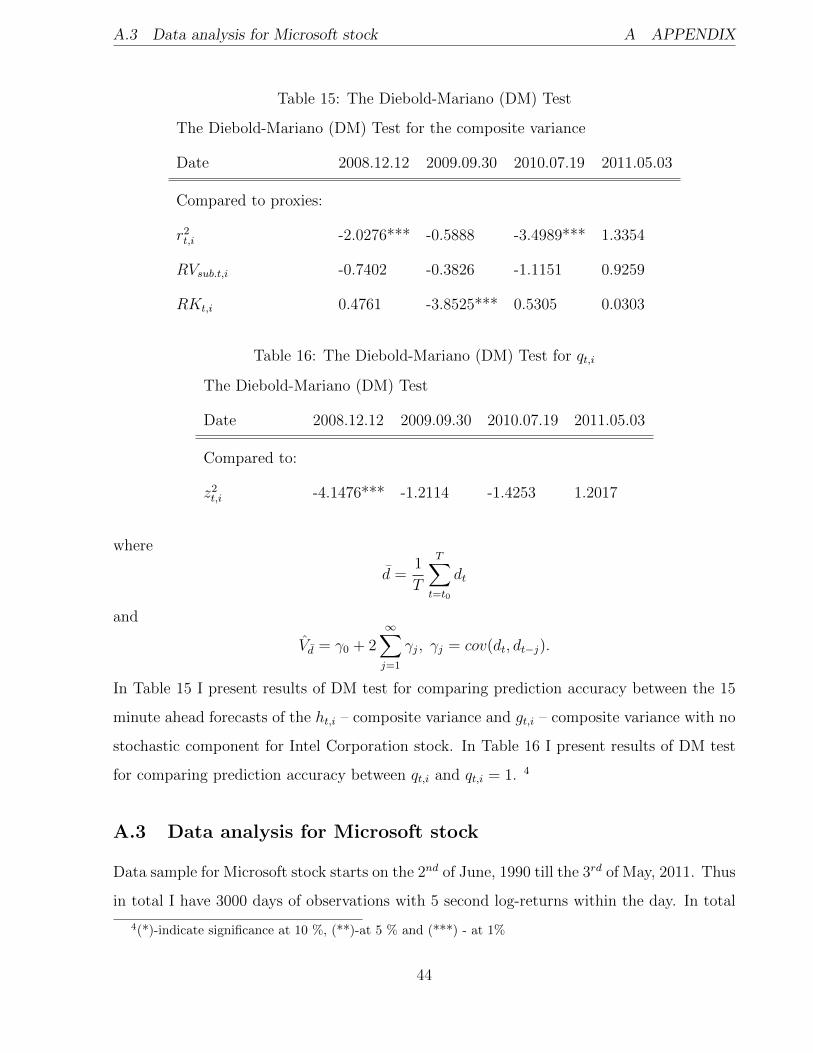
Table 15: The Diebold-Mariano (DM) Test
The Diebold-Mariano (DM) Test for the composite variance
Date 2008.12.12 2009.09.30 2010.07.19 2011.05.03
Compared to proxies:
r2t,i -2.0276*** -0.5888 -3.4989*** 1.3354
RVsub.t,i -0.7402 -0.3826 -1.1151 0.9259
RKt,i 0.4761 -3.8525*** 0.5305 0.0303
Table 16: The Diebold-Mariano (DM) Test for qt,i
The Diebold-Mariano (DM) Test
Date 2008.12.12 2009.09.30 2010.07.19 2011.05.03
Compared to:
z2t,i -4.1476*** -1.2114 -1.4253 1.2017
where
d =1
T
T∑t=t0
dt
and
Vd = γ0 + 2∞∑j=1
γj, γj = cov(dt, dt−j).
In Table 15 I present results of DM test for comparing prediction accuracy between the 15
minute ahead forecasts of the ht,i – composite variance and gt,i – composite variance with no
stochastic component for Intel Corporation stock. In Table 16 I present results of DM test
for comparing prediction accuracy between qt,i and qt,i = 1. 4
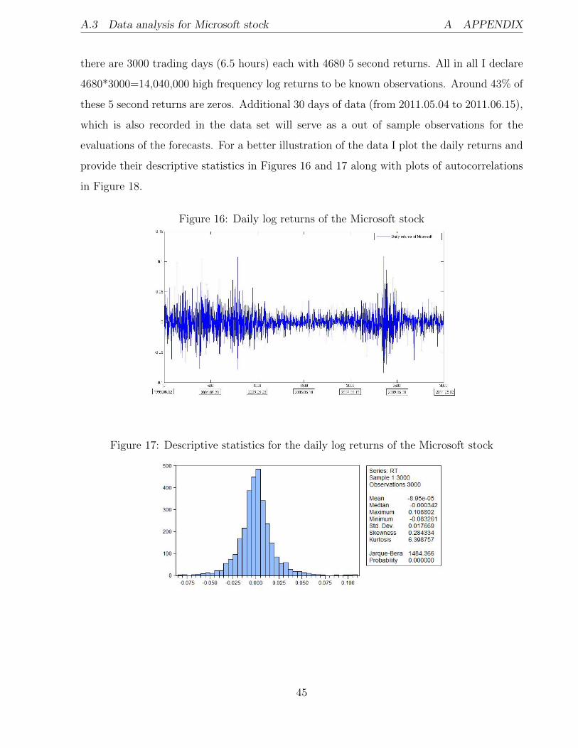
A.3 Data analysis for Microsoft stock
Data sample for Microsoft stock starts on the 2nd of June, 1990 till the 3rd of May, 2011. Thus
in total I have 3000 days of observations with 5 second log-returns within the day. In total
4(*)-indicate significance at 10 %, (**)-at 5 % and (***) - at 1%
44
A.3 Data analysis for Microsoft stock A APPENDIX
there are 3000 trading days (6.5 hours) each with 4680 5 second returns. All in all I declare
4680*3000=14,040,000 high frequency log returns to be known observations. Around 43% of
these 5 second returns are zeros. Additional 30 days of data (from 2011.05.04 to 2011.06.15),
which is also recorded in the data set will serve as a out of sample observations for the
evaluations of the forecasts. For a better illustration of the data I plot the daily returns and
provide their descriptive statistics in Figures 16 and 17 along with plots of autocorrelations
in Figure 18.
Figure 16: Daily log returns of the Microsoft stock
Figure 17: Descriptive statistics for the daily log returns of the Microsoft stock
45

A.4 Results for Microsoft stock A APPENDIX
Figure 18: Autocorrelation for the squared daily returns of the Microsoft stock
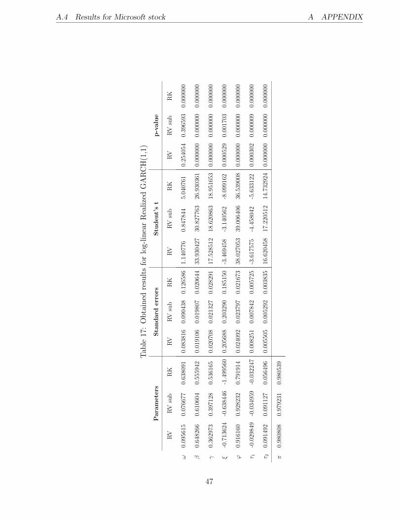
A.4 Results for Microsoft stock
In order to check whether or not results obtained for Intel Corporation are robust I carry out
the same analysis for the Microsoft stock. Microsoft and Intel Corporation stocks have very
similar trading frequency, in fact in my dataset these two stocks are the most often traded.
Therefore, the results should be similar (summarized results for the Microsoft can be found
in Tables :18, 17, 19, 20,21, 23, 25, 22, 24 and Figure 19).
After close investigation of the results one noticeable difference is the higher significance of
the forecasts for the Microsoft stock. Other than that the results are very similar for the
both stocks. Therefore the same conclusions can be drawn and this serves as a robustness
check for the results obtained for the Intel Corporation stock.
A.4.1 Realized GARCH results
46
A.4 Results for Microsoft stock A APPENDIX
Tab
le17
:O
bta
ined
resu
lts
for
log-
linea
rR
ealize
dG
AR
CH
(1,1
)
Para
mete
rsS
tan
dard
err
ors
Stu
dent’
st
p-v
alu
e
RV
RV
sub
RK
RV
RV
sub
RK
RV
RV
sub
RK
RV
RV
sub
RK
ω0.
0956
150.
0766
770.
6380
910.
0838
160.
0904
380.
1265
861.
1407
760.
8478
445.
0407
610.
2540
540.
3965
930.
0000
00
β0.
6482
660.
6106
040.
5559
420.
0191
060.
0198
070.
0206
4433
.930
427
30.8
2776
326
.930
361
0.00
0000
0.00
0000
0.00
0000
γ0.
3629
730.
3971
280.
5361
650.
0207
080.
0213
270.
0282
9117
.528
512
18.6
2086
318
.951
653
0.00
0000
0.00
0000
0.00
0000
ξ-0
.713
624
-0.6
3844
6-1
.499
560
0.20
5688
0.20
3290
0.18
5150
-3.4
6945
8-3
.140
562
-8.0
9916
20.
0005
290.
0017
030.
0000
00
ϕ0.
9161
600.
9282
320.
7919
140.
0240
920.
0237
970.
0216
7338
.027
053
39.0
0640
636
.539
008
0.00
0000
0.00
0000
0.00
0000
τ 1-0
.029
849
-0.0
3495
9-0
.032
247
0.00
8251
0.00
7842
0.00
5725
-3.6
1757
5-4
.458
042
-5.6
3312
20.
0003
020.
0000
090.
0000
00
τ 20.
0914
920.
0911
270.
0564
960.
0055
050.
0052
920.
0038
3516
.620
458
17.2
2051
214
.732
924
0.00
0000
0.00
0000
0.00
0000
π0.
9808
080.
9792
310.
9805
39
47

A.4 Results for Microsoft stock A APPENDIX
Table 18: Log-likelihood for log-linear Realized GARCH(1,1)
Realized measure: RV RV sub RK
Value of the log-likelihood: 12155.3449 12317.2870 13253.8499
Table 19: Obtained results for out of sample forecasts of daily volatility and realized measure
over 30 days horizon
RV RV sub RK
Forecasts for: ht xt ht xt ht xt
RMSE: 1.07E-04 1.06E-04 1.24E-04 1.28E-04 7.01E-05 1.00E-04
Compared to out of sample: RVt RVsub.t RKt
A.4.2 Multiplicative Component GARCH results
Table 20: GARCH(1,1) results for stochastic component qt,i
Parameter value Standard error Student’s t p-value
ω 0.059516 0.022729 2.618532 0.014305
α 0.093866 0.021823 4.301170 0.000199
β 0.847342 0.034912 24.270579 0.000000
Value of the log-likelihood 1102.1942
48
A.4 Results for Microsoft stock A APPENDIX
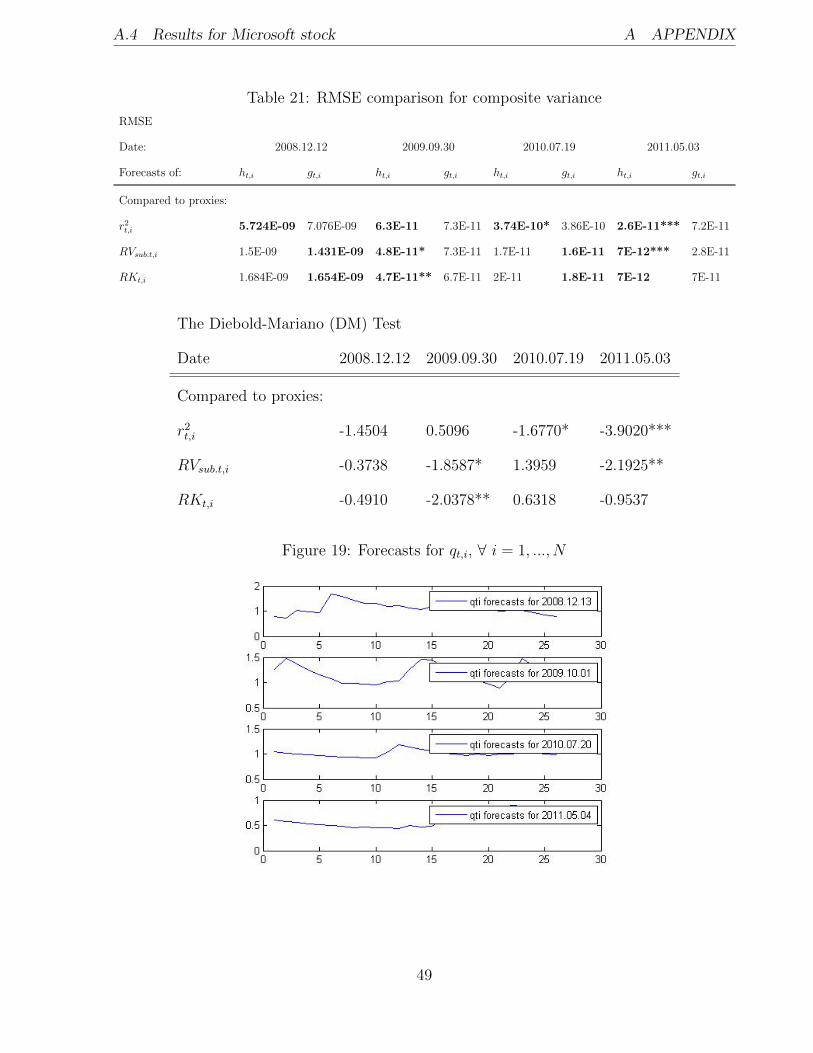
Table 21: RMSE comparison for composite variance
RMSE
Date: 2008.12.12 2009.09.30 2010.07.19 2011.05.03
Forecasts of: ht,i gt,i ht,i gt,i ht,i gt,i ht,i gt,i
Compared to proxies:
r2t,i 5.724E-09 7.076E-09 6.3E-11 7.3E-11 3.74E-10* 3.86E-10 2.6E-11*** 7.2E-11
RVsub.t,i 1.5E-09 1.431E-09 4.8E-11* 7.3E-11 1.7E-11 1.6E-11 7E-12*** 2.8E-11
RKt,i 1.684E-09 1.654E-09 4.7E-11** 6.7E-11 2E-11 1.8E-11 7E-12 7E-11
The Diebold-Mariano (DM) Test
Date 2008.12.12 2009.09.30 2010.07.19 2011.05.03
Compared to proxies:
r2t,i -1.4504 0.5096 -1.6770* -3.9020***
RVsub.t,i -0.3738 -1.8587* 1.3959 -2.1925**
RKt,i -0.4910 -2.0378** 0.6318 -0.9537
Figure 19: Forecasts for qt,i, ∀ i = 1, ..., N
49
A.4 Results for Microsoft stock A APPENDIX
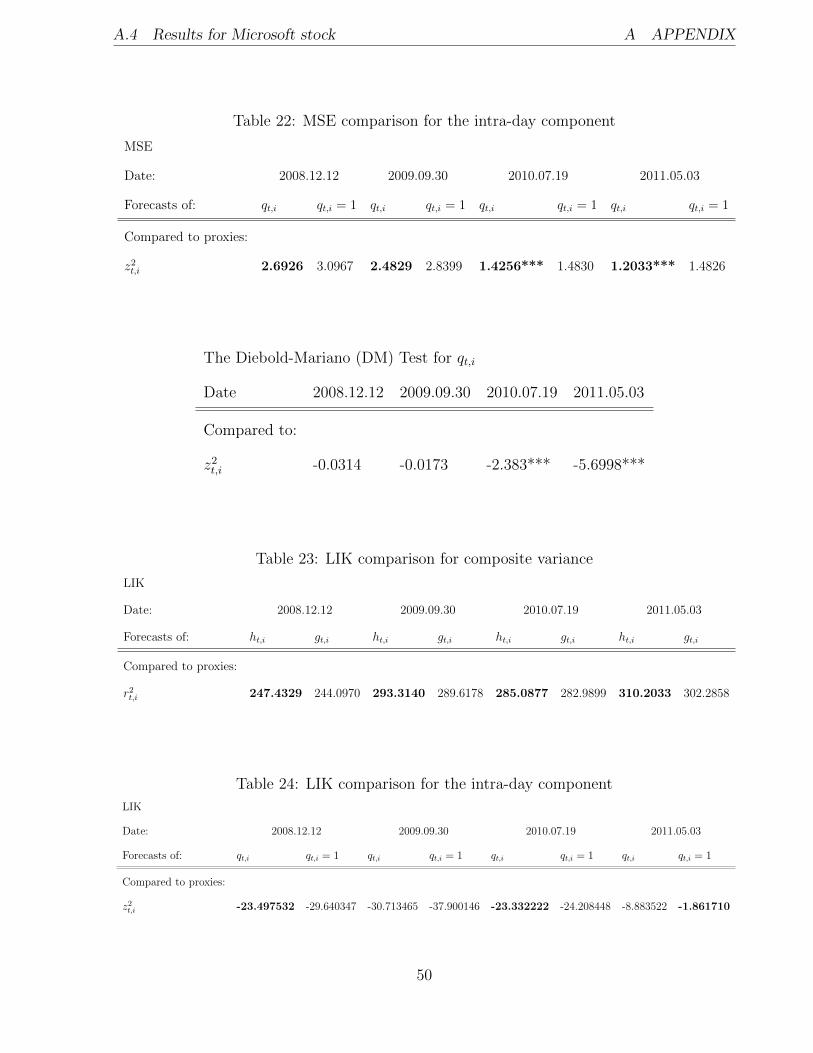
Table 22: MSE comparison for the intra-day component
MSE
Date: 2008.12.12 2009.09.30 2010.07.19 2011.05.03
Forecasts of: qt,i qt,i = 1 qt,i qt,i = 1 qt,i qt,i = 1 qt,i qt,i = 1
Compared to proxies:
z2t,i 2.6926 3.0967 2.4829 2.8399 1.4256*** 1.4830 1.2033*** 1.4826
The Diebold-Mariano (DM) Test for qt,i
Date 2008.12.12 2009.09.30 2010.07.19 2011.05.03
Compared to:
z2t,i -0.0314 -0.0173 -2.383*** -5.6998***
Table 23: LIK comparison for composite variance
LIK
Date: 2008.12.12 2009.09.30 2010.07.19 2011.05.03
Forecasts of: ht,i gt,i ht,i gt,i ht,i gt,i ht,i gt,i
Compared to proxies:
r2t,i 247.4329 244.0970 293.3140 289.6178 285.0877 282.9899 310.2033 302.2858
Table 24: LIK comparison for the intra-day component
LIK
Date: 2008.12.12 2009.09.30 2010.07.19 2011.05.03
Forecasts of: qt,i qt,i = 1 qt,i qt,i = 1 qt,i qt,i = 1 qt,i qt,i = 1
Compared to proxies:
z2t,i -23.497532 -29.640347 -30.713465 -37.900146 -23.332222 -24.208448 -8.883522 -1.861710
50
A.4 Results for Microsoft stock A APPENDIX
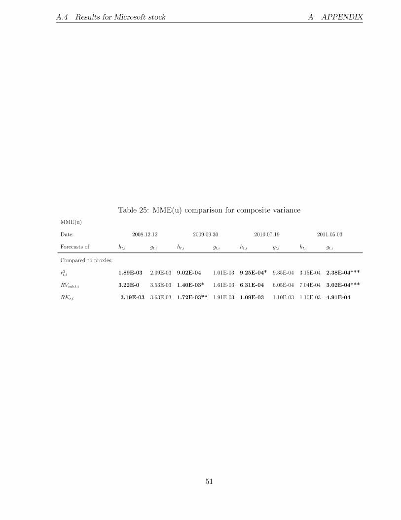
Table 25: MME(u) comparison for composite variance
MME(u)
Date: 2008.12.12 2009.09.30 2010.07.19 2011.05.03
Forecasts of: ht,i gt,i ht,i gt,i ht,i gt,i ht,i gt,i
Compared to proxies:
r2t,i 1.89E-03 2.09E-03 9.02E-04 1.01E-03 9.25E-04* 9.35E-04 3.15E-04 2.38E-04***
RVsub.t,i 3.22E-0 3.53E-03 1.40E-03* 1.61E-03 6.31E-04 6.05E-04 7.04E-04 3.02E-04***
RKt,i 3.19E-03 3.63E-03 1.72E-03** 1.91E-03 1.09E-03 1.10E-03 1.10E-03 4.91E-04
51