Forthcoming, Journal of Fixed Income

The Risk in Fixed-Income Hedge Fund Styles

By

William FungAnd

David A. Hsieh

August 2002

William Fung is Visiting Research Professor of Finance, Centre for Hedge FundResearch and Education, London Business School. Phone: 201-847-0090. Fax: 201-847-0004. Email: wkhf1@aol.com

David A. Hsieh is Professor of Finance, Fuqua School of Business, Duke University.Phone: 919-660-7779. Fax: 919-660-7961. Email: david.a.hsieh@duke.edu

We acknowledge the LBS Centre for Hedge Fund Research and Education for providingthe hedge fund data used in this paper. Earlier versions of this paper were presented atPrinceton University, Boston University, New York University, NBER Risk of FinancialInstitutions Workshop, and Vanderbilt University. We thank Wayne Ferson and StanleyKon for detailed comments and suggestions on earlier drafts.

2

Abstract

This paper studies the risk in fixed-income hedge fund styles. Principal componentanalysis is applied to groups of fixed-income hedge funds to extract common sources ofrisk and return. These common sources of risk are related to market risk factors, such aschanges in interest rate spreads and options on interest rate spreads. We call these asset-based style factors (“ABS”). The paper finds that fixed-income hedge funds tend to beexposed to a common ABS factor: credit spreads.

Hedge fund strategies came under intense scrutiny in the wake of the stressful

market events surrounding the collapse of Long-Term Capital Management (LTCM).

Several studies have been sponsored by regulatory agencies of financial markets: the

President’s Working Group on Financial Markets [1999], and Bank for International

Settlements [1999a, b, and c]. In addition to the macro question as to whether hedge

funds have a destabilizing influence on markets, these studies directed much of their

attention to a particular type of strategy used by fixed-income hedge funds: Convergence

Trading. Just what are the risk characteristics that caught the attention of financial

regulators and how do they differ from other hedge fund strategies?

Understanding hedge fund risk is a non-trivial task. Information on hedge funds

is hard to come by. As private investment vehicles, hedge funds1 are exempt from the

disclosure requirements on publicly traded companies and mutual funds. Although the

hedge fund industry is gradually shifting towards greater disclosure, there is still a need

to model the link between hedge fund returns and asset returns. Hedge fund managers

rarely disclose their trading strategies. This leaves researchers with the daunting task of

modeling highly complex strategies with incomplete data sets. Challenging as it seems,

the rewards can be substantial. A model like this will allow hedge fund investors and

counterparties to identify and explicitly measure the different types of hedge fund risk.

By linking these strategy risks to asset prices with long histories, we may even be able to

predict hedge fund returns during market extremes.

A number of steps must be taken to achieve this. First, we need to extract

common risk factors in groups of fixed-income hedge funds. Typically, hedge funds are

grouped by “location” and “strategy.” Location refers to “where” a manager trades, such

4

as stocks, bonds, commodities, or currencies. Strategy refers to “how” a manager trades,

such as buy-and-hold, long-short, trend following, etc. Style refers to a combination of

location and strategy, such as buy-and-hold on stocks or trend following on currencies.

In this paper, we use the peer groupings of Hedge Fund Research (HFR), a vendor of

hedge fund data. Since funds that use similar styles have correlated returns, their

common styles can be extracted by principal component analysis. These common styles

are called style factors.

Second, we link the extracted style factors to observable market prices. Here, we

follow the method of using asset-based style (“ABS”) factors to model hedge fund

returns; see Fung and Hsieh [2002] for a detailed discussion on asset-based hedge fund

style factors. Fung and Hsieh [2001] showed theoretically that trend-following strategies

can be represented as an option strategy, in particular, a long position on lookback

straddles in the major asset markets. We verified empirically that returns of trend-

following funds are strongly correlated to returns of lookback straddles. In addition,

Mitchell and Pulvino [2001] simulated the returns of a merger arbitrage strategy applied

to announced takeover transactions from 1968 until 1998. This strategy generated returns

that are similar to those of merger arbitrage funds. In this paper, we directly model

convergence trading with options, to explain the returns of fixed-income funds.2

The benefits of ABS factors are threefold. First, ABS factors can be applied to

create performance benchmarks that depend solely on observable prices. This allows

investors to directly assess a hedge fund’s performance based on its strategy

characteristics rather than indirectly through peer-group averages that may include funds

using different strategies.3 Second, ABS factors based on observable prices typically

5

have longer histories than the hedge funds themselves. This is particularly helpful in

modeling the risk of hedge fund investing under alternative scenarios that may otherwise

be obscured by the short history of hedge fund returns.4 Third, from these explicit links,

expected returns of hedge fund strategies can be directly linked to expected returns of the

underlying assets. Therefore, in a unified framework, ABS factors can be used to answer

questions on ex-post performance evaluation, risk management and return prospects of a

hedge fund strategy.

The paper proceeds as follows. Section I discusses the data for fixed-income

hedge funds. Section II discusses the distinctive risk characteristics of convergence

trading. Convergence trading bets on the relative price between two assets to narrow (or

converge), in which "approximately offsetting positions are taken in two securities that

have similar, but not identical, characteristics and trade at different prices." [BIS, 1999c,

p. 11].5

Unlike riskless arbitrage, convergence trading is risky, because the relative price

of these assets can just as easily diverge. This is particularly so with fixed-income

applications of convergence trading. Unlike stocks where the dominant risk factor is the

systematic market component, fixed-income securities can have several important risk

factors beyond just the level of interest rate. This is especially important under stressful

market conditions where these risk factors can move in opposite directions.

For example, a convergence trade involving a long position on mortgages-backed

securities (MBS for short) and a short position on treasuries will incur large losses if the

interest rate spread between MBS and treasuries widen dramatically. This can occur

during extreme market conditions when there is a flight to quality pushing up prices of

6

treasuries while depressing credit sensitive securities at the same time. We believe this

characteristic together with the liberal use of leverage on illiquid securities by fixed-

income convergence funds are the primary causes of concern for financial regulators.

Our evidence is based on convergence trading in hedge funds. In particular, we focus on

fixed-income hedge funds, some of which ran into substantial financial difficulties in the

fall of 1998.6

Section III extracts common risk factors from the fixed-income hedge funds in the

HFR database, and links them to ABS factor. Section IV provides evidence that these

ABS factors also show up in a sample of fixed-income hedge funds from the TASS

database. Section V checks if these ABS factors for fixed-income hedge funds show up

in fixed-income mutual funds. Concluding remarks are in section VI of the paper.

I. DATA FOR FIXED-INCOME HEDGE FUNDS

In this paper, we use the fixed-income hedge funds in the HFR database. As of

December 2000, the HFR database has 1,400 individual hedge funds with $117 billion of

assets under management. HFR groups hedge funds into roughly 30 style indices.

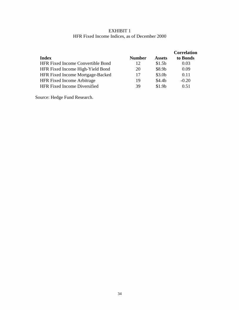
Nearly 8% of the funds with 17% of the assets are in five indices for fixed-income hedge

funds listed in Exhibit 1.

Fixed-Income Convertible Bond funds invest primarily in convertible bonds.7

Fixed-Income High-Yield Bond funds invest in non-investment grade debt. Fixed-

Income Mortgage-Backed funds invest in mortgage-backed securities (including

collateralized mortgage obligations, real estate mortgage investment conduits, and

stripped mortgage-backed securities), typically hedging the interest rate risk and

7

prepayment risk. Fixed-Income Arbitrage is a strategy that exploits pricing inefficiencies

between related fixed-income securities while hedging exposure to interest rate risk.

Fixed-Income Diversified funds either use multi-strategy or niche strategies. Their

returns have low correlation to bond returns, as measured by the Lehman Aggregate

Bond index.

As in Fung and Hsieh [1997, 2001], common styles among hedge funds in each

grouping are extracted using a principal component analysis8. The idea is that funds that

have the same style (i.e. location and strategy) will have correlated returns. For this

analysis, we use all funds that have returns between 1998 and 2000. The choice of the

time period is motivated by practical considerations. We keep the data in 2001 as a

holdout sample to validate our empirical findings, consequently the data analysis ended

in 2000. Starting the analysis earlier than 1998 would greatly reduce the number of funds

that have return data for the entire period.

The amount of cross-sectional variance explained by the first three principal

components in each of the five groups is given in Exhibit 2. Three groups of fixed-

income hedge funds (Convertible, High-Yield, and Mortgage-Backed) have only one

common style. The respective first principal component explains more than 50% of the

cross-sectional variation in returns. In contrast, two other groups of fixed-income hedge

funds (Arbitrage and Diversified) appear to have two or more common styles. The

respective first principal component explains roughly 35% of the cross-sectional variation

in returns, while the second component explains over 20% of return variation cross-

sectionally.

8

We call these components return-based style factors to emphasize the dominant

source of input in their construction. In the next section, we extend the analysis to link

these return-based style factors to observable market risk factors that are exogenous to

the hedge fund returns data.

II. ABS FACTORS FOR FIXED-INCOME HEDGE FUNDS

Using the qualitative descriptions of the fixed-income hedge funds styles, we

postulate a variety of benchmark returns using observed asset prices. We call these ABS

factors.

Each ABS factor involves a pair of key variables--“location” and “strategy.” We

define location as the type of securities to which a hedge fund manager applies his or her

strategy. In other words, where a manager trades. Locations for fixed-income hedge

funds are typically defaultable bonds (such as high-yield bonds, convertible bonds,

corporate bonds), mortgages, asset-backed securities, and agencies and treasuries.

In terms of strategy, we consider four main types: long-only, passive spread

trading, trend following and convergence trading. For long-only strategies, we use

standard fixed-income benchmarks such as the CSFB Convertible Bond index return,

CSFB High-Yield Bond index return, the Lehman Mortgage-Back index return, JP

Morgan Emerging Market Bond index return, etc. Here, the ABS factor is simply the

index return itself, which completely characterizes a passive buy-and-hold strategy in that

location.

For passive spread trading, the ABS factor is the difference between two bond

index returns. Examples are the convertible bonds-minus-treasury return, the mortgage

9

bond-minus-treasury return, the high-yield bond-minus-treasury return, and the emerging

market bond-minus-treasury return.

In the case of trend-following strategies on spreads, the ABS factor is a lookback

straddle on the difference between two interest rates.9 Fung and Hsieh [2001] provided a

general model for trend-following strategies on individual assets (such as stock indices,

government bonds, short term interest rates, foreign currencies, and commodities) using

lookback straddles. Here, we extend the application to spreads between two interest rates

(or two assets, more generally).

The innovation in this study is the creation of an ABS factor for convergence

trading. The term convergence trading refers to trading strategies that bet on the price

difference between two assets will narrow (or converge) in the future. A convergence

trade generally involves buying (going long) the cheaper asset and selling (going short)

the more expensive asset. The trades are reversed when the prices of the two assets

become more similar.

The genesis of convergence trading is riskless arbitrage. Riskless arbitrage is the

activity that enforces the law of one price, which states that two assets with the same

payoffs in every state of the world must have identical prices. If the law of one price is

violated, riskless arbitrage profit obtains by buying (going long) the cheaper asset and

selling (going short) the more expensive asset. This locks in the difference between the

two asset prices. There is no risk in this trade, since the payoffs of the two assets are

identical in every state, so the payoffs from the long position can be used to offset the

payoffs of the short position. Well-known examples are the triangular arbitrage and

10

covered interest arbitrage in the foreign exchange markets, cash-futures arbitrage in the

futures market, and coupon-STRIPS arbitrage in the US treasury securities market.

As a general class of strategy, convergence trading is founded on a variation to

the law of one price. Here, theory states that two assets with similar payoffs in most

states of the world should have similar prices.10 If the two similar assets have very

different prices, then convergence traders would buy (go long) the cheaper asset and sell

(go short) the more expensive one. Even though many convergence trading strategies

contain the word arbitrage, they all involve some risk, since the payoff from the long

position is not always sufficient to cover the payoff for the short position. The

convergence trade is a bet that the expected payoff is more than sufficient to compensate

for the risk of any loss.

To model convergence trading, we need a description of the entry and exit points.

Let S(t) be the price of an asset or a group of assets. A convergence trader believes that

S(t) will not move very far away from some price level, say Smid. If S(t) is sufficiently

below Smid, a long position in the asset is initiated. If S(t) is sufficiently above Smid, a

short position in the asset is initiated. For ease of notation, we denote the trigger price S

(Sh) to be the price below (above) which the convergence trader will go long (short) the

asset.

A fully specified theoretical model of convergence trading strategies would

require explicit knowledge of the key prices Smid, S , and Sh . This is difficult to do, since

hedge fund managers, being protective of their proprietary skills, generally do not

disclose their trading rules. To circumvent this problem, we make use of an option

strategy to eliminate the need to specify these prices.

11

The option strategy comes from the following intuition. The convergence trading

strategy is basically the opposite of the trend-following strategy. A trend-following

strategy tries to capture a large price move, up or down. Typically, the trend follower

observes a trend by waiting for the price of an asset to exceed certain thresholds. When

the asset price goes above (below) the given threshold, a long (short) position in the asset

is initiated. Assuming that the same set of key prices are used, the trend-following trader

and the convergence trader will have similar entry and exit decisions but in exact

opposite positions.

Instead of modeling the myriad of possible entry and exit decisions of trend-

following strategies, Fung and Hsieh [2001] modeled its payoff as a long position in a

lookback straddle. Briefly, a lookback straddle is a pair of structured options. The

lookback call option gives the owner the right (but not the obligation) to purchase an

asset at the lowest price during the life of the option. The lookback put option gives the

owner the right (but not the obligation) to sell an asset at the highest price during the life

of the option. The theoretical pricing of a European-style lookback option is in Goldman,

Sosin, and Gatto [1979]. The lookback straddle consists of both the lookback call and

lookback put. Given a sample period and a reference asset, the payout of the lookback

straddle on that asset is the maximum any trend-following strategy can achieve. The

question is the attendant cost (the lookback option’s premium) to achieve this maximum

payout. Alternative trend-following strategies can be represented by variations to the

entry/exit prices of those used in the lookback straddle. These variations will result in

less payout than the lookback straddle, but should also involve less cost to implement

12

than the lookback option’s premium. These are the key considerations in choosing a

particular form of trend-following strategy.

Since the convergence trading strategy is the opposite of the trend-following

strategy, the convergence trading strategy can be modeled as a short position in a

lookback straddle. In other words, the spread position of the convergence trade is

identical to the negative of the ‘delta’ of the lookback straddle.11

This “primitive” convergence trading strategy can differ from the actual strategy

used by a convergence trader. If the trader has a superior trading rule, it should generate

better performance (i.e. positive “alpha”) than the primitive convergence trading strategy.

The last theoretical issue is the horizon of the convergence trade. Since we have

no good information on this, we will use two extremes: a 1-month and a 10-year

horizon.12 As data on structured options are not readily available, we simulate their

returns, illustrated for the 1-month lookback straddle, as follows.

For a given interest rate spread (e.g. the yield on Moody’s Baa corporate bonds

minus the yield on 10 year treasury bonds), we start with the daily spread. At the

beginning of each month, we purchase a lookback straddle on the spread. The price of

the straddle is based on the theoretical pricing formula in Goldman, Sosin, and Gatto

[1979], using the historical volatility of the spread for the previous 21 trading days. At

the end of the month, the payoff of the lookback straddle is the difference between the

maximum and minimum spreads during the month. The return of the straddle equals the

payoff, divided by the cost of the straddle, minus one. Using this procedure, we simulate

the returns of lookback straddles for four spreads: Moody’s Baa bond yield minus the 10-

year treasury rate (“Baa/treasury spread”), Merrill Lynch’s High-Yield bond rate minus

13

the 10-year treasury rate (“high-yield/treasury spread”), Lehman’s mortgage yield minus

the 10-year treasury rate (“mortgage/treasury spread”), and Intercapital 10-year swap

rate minus the 10-year treasury rate (“swap/treasury spread”). In each case, the 10-year

treasury rate is the 10-year constant maturity interest rate in the Federal Reserve’s H15

Statistical Release. For the 10-year lookback straddles, we start these options in January

1994, and reprice the options at the end of each subsequent month. The straddle returns

are the percentage price changes during each month. The returns of these lookback

straddles are the asset-based benchmarks we use for convergence fixed-income funds.

Note that it is possible for the returns of lookback straddles (which are dynamic

spread positions) to be highly correlated to the returns on static spread positions in a

given sample period. This happens when the lookback straddle has a long horizon and

the underlying spread has widened or narrowed persistently during the sample period.

For example, high-yield/treasury spreads and mortgage/treasury spreads have generally

risen since mid-1998. In this case, it is difficult to distinguish, statistically, between a

static position and a convergence position in these two spreads.

III. LINKING RETURN-BASED STYLE FACTORS TO ASSET-BASED STYLE

FACTORS

In this section, we link the return-based style factors of fixed-income hedge funds

(extracted by principal components in Section I) to ABS factors described in Section II.

The process for identifying the appropriate ABS factors can be summarized as follows.

First, funds are sorted into groups according to HFR’s qualitative style designations and

return-based style factors for each group are established via principal components

14

analyses of the funds’ returns as described in Section I. Second, Sharpe ‘s (1992) asset

class model is used to determine the location of these return-based style factors,

regressing the factors’ monthly returns to various commonly used asset benchmarks.

Third, an additional set of analysis is carried out to detect the presence of nonlinear,

dynamic trading strategies such as trend following and convergence trading. From these

analyses, ABS factors for each group of funds are identified. Finally, an out-of-sample

test on the explanatory power of these ABS factors is reported.

Fixed-Income Convertible Bond Hedge Funds

As of July 2001, the HFR database contains twelve operational and four defunct

funds in the Fixed-Income Convertible Bond peer group (as distinct from the HFR

Convertible Arbitrage peer group). These funds have one common style as shown in

Section I. For this group of funds, we use the HFR Fixed-Income Convertible Bond

peer-group average as the return-based style factor, which has a correlation of 0.932 with

the first principal component.

Next, this return-based style factor is linked to ABS factors via the Sharpe [1992]

asset class model by regressing its monthly returns on various benchmarks. Based on

HFR’s description that this group of funds, being “primarily long only convertible

bonds,” 13 we use the CSFB Convertible Bond index return and the difference between

the CSFB Convertible Bond index return and the Lehman Treasury Bond index return

(“convertible bond-minus-treasury” return) as benchmarks.14 While the return-based style

factor has a correlation of 0.824 with the CSFB Convertible Bond index returns, the

convertible bond-minus-treasury returns have stronger explanatory power in a joint

15

regression of the two variables. The linear relationship is shown in Exhibit 3 and the R²

is 0.70. A summary of the regression is in Exhibit 4.

To detect the presence of nonlinear, dynamic trading strategies, returns from

lookback straddles on the convertible/treasury spread are added to the set of regressors

alongside the returns from lookback straddles on the Baa/treasury spread, high-

yield/treasury spread, and swap/treasury spread to the regression. Short-horizon and

long-horizon lookback straddles on these variables are introduced to the regression

separately in order to avoid multicollinearity. In both cases, the static convertible bond-

minus-treasury return remains the dominant regressor. The only statistically significant

regressor is the short-horizon lookback straddle on the swap/treasury spread, which has a

negative coefficient and is consistent with the presence of convergence trading.

However, the increment in R² is rather modest, from 0.70 to 0.75, which indicates that

Convertible Bond funds have primarily non-directional static exposure to long positions

in convertible bonds hedged with short positions in U.S. treasuries, with a small amount

of short-horizon convergence trading.

To corroborate this analysis, we examine the out-of-sample correlation between

the return-based style factor’s returns and the convertible bond-minus-treasury returns.

As shown in Exhibit 5, the linear relationship continues to hold in 2001. This behavior is

consistent with the view that Convertible Bond funds do not use dynamic trading

strategies. Empirical support for this assertion can be seen from the fact that convertible

bonds have generally outperformed treasuries from October 1990 until January 2001,

with the exception of August/September 1998. Since the beginning of 2001, convertible

bonds have underperformed treasuries. If Convertible Bond funds followed dynamic

16

trading strategies, they would have switched from long convertible/short treasury to long

treasury/short convertible and their returns would not have a strong correlation to the

convertible bond-minus-treasury return in 2001.

Fixed-Income High-Yield Hedge Funds

As of July 2001, the HFR database contains twelve operational and four defunct

funds belonging to the Fixed-Income High-Yield peer group. These funds have one

common style as shown in Section I. We use the HFR Fixed-Income High-Yield peer-

group average as a proxy of the return-based style factor. This proxy has a return

correlation of 0.874 with the returns of the first principal component.

Next, Sharpe’s [1992] style regression is used to determine the location of these

funds. The HFR Fixed-Income High-Yield peer-group average has a correlation of 0.853

with the CSFB High-Yield Bond index return, which is consistent with HFR’s

description of this group of funds to “invest in non-investment grade debt.” However, in

a joint regression of the peer-group average against both the high-yield bond return and

the high-yield bond-minus-treasury return, the latter has the dominant statistical

explanatory power. The linear relationship is shown in Exhibit 6. (The R² is 0.78. A

summary of the regression is in Exhibit 4.)

To detect the presence of nonlinear, dynamic trading strategies, returns from

short-horizon and long-horizon lookback straddles on the high-yield/treasury spread are

added to the set of regressors separately in order to avoid multicollinearity. Interestingly,

both straddles have negative coefficients, which is consistent with the presence of

convergence trading. The high-yield bond-minus-treasury return statistically dominates

17

the short-horizon straddle but is statistically dominated by the long-horizon straddle. If

we use the long-horizon straddle as the sole regressor, the R² is 0.79. Prima facie, this

group of funds has mainly non-directional exposure to long positions in high-yield bonds

hedged with short positions in U.S. treasuries. However, the correlation of the long-

horizon high-yield/treasury spread lookback straddle return is 0.942 with the high-yield

bond-minus-treasury return. Thus, it is not clear if the strategy is better described

empirically by a dynamic, long-horizon convergence trading strategy than static exposure

to the spread.

To answer this question, observe that high-yield bonds outperformed treasuries

from Jan 1991 until Dec 1999, but have generally underperformed treasuries since Jan

2000. Similarly, High-Yield funds performed well during the first period (averaging 1%

per month), but poorly in the second period (averaging 0.09% per month). This would

point to a passive exposure to a long high-yield/short treasury position than a dynamic,

convergence trading strategy.

To corroborate this analysis, we examine the out-of-sample correlation between

this group’s return-based style factor’s returns and the high-yield bond-minus-treasury

returns. As shown in Exhibit 7, the linear relationship continues to hold in 2001. One

plausible explanation to these empirical observations may be consistent with time-

varying betas from changes in leverage on a long high-yield/short treasury position as

distinct from trend-following where betas with respect to the underlying variable can

fluctuate from positive to negative dynamically.

Fixed-Income Mortgage-Backed Hedge Funds

18

As of July 2001, the HFR database has nineteen operational and ten defunct funds

belonging to the Fixed-Income Mortgage-Backed peer group. These funds have one

common style as shown in Section I. We use the HFR Fixed-Income Mortgage-Backed

peer-group average to proxy the return-based style factor. This proxy has a return

correlation of 0.949 with the returns of the group’s first principal component.

The key features of HFR’s description of this group of funds are--“invest in

mortgage-backed securities,”and “hedging of prepayment risk and interest rate risk is

common.” The return-based style factor has a low correlation (-0.194) with the change in

the mortgage yields (based on the Lehman Mortgage-Backed Index), while the

correlation is higher (–0.411) with the change in the mortgage/treasury spread. In the

Sharpe [1992] style regression, we find that three interest rate variables are needed to

explain the returns of these funds: change in mortgage rate, change in the 10-year swap

rate, and change in the 10-year treasury rate. The R² is 0.59. A summary of the

regression is in Exhibit 4.

To detect the presence of nonlinear, dynamic trading strategies, returns from

lookback straddles on the mortgage/treasury spread and swap/treasury spread are added

to the set of regressors. Short-horizon and long-horizon lookback straddles on these

variables are introduced to the regression separately in order to avoid multicollinearity.

The short-horizon straddles do not increase the explanatory power of the regression, but

the long-horizon straddles add explanatory power. In fact, the R² improves to 0.66 if we

use the long-horizon straddles in swap/treasury spread and mortgage/treasury spread

along with the change in mortgage rate. Interestingly, the swap/treasury spread straddle

has a positive sign (consistent with trend following) and the mortgage/treasury spread

19

straddle has a negative sign (consistent with convergence trading). Exhibit 8 shows that

the relationship between the return-based style factor and the fitted value of the

regression. The graph is roughly linear.

The out-of-sample predictive power of this regression model, however, is poor.

Exhibit 9 shows that this relationship did not adequately describe the return-based style

factor in 2001. More work is needed to explain this empirical phenomenon.

Fixed-Income Arbitrage Hedge Funds

As of July 2001, the HFR database includes 16 operational and 27 defunct funds

belonging to the Fixed-Income Arbitrage peer group. As shown in Section I, these funds

have a least two common styles. We use the first two principal components to directly

proxy the return-based style factors of these styles.

HFR describes these funds as using “a market neutral hedging strategy that seeks

to profit by exploiting pricing inefficiencies between related fixed-income securities

while neutralizing exposure to interest rate risk.” Indeed, the HFR Fixed-Income

Arbitrage peer-group average has low correlation with the major bond indices.15

The Sharpe [1992] style analysis shows that the first principal component is

strongly correlated to high-yield bond-minus-treasury returns, consistent with non-

directional exposures to interest rates. Exhibit 10 shows that the relation is basically

linear. (The R² is 0.50.) There are two outliers in the fall of 1998. We noted in the earlier

discussion of Fixed-Income High-Yield funds that the returns of long-horizon lookback

straddles on the high-yield/treasury spread has a high correlation (0.942) with high-yield

bond-minus-treasury returns. A regression with both variables indicates that they have

20

the same explanatory power. The straddle has a negative sign, consistent with

convergence trading. Hence, the first principal component is primarily non-directional

exposure to spreads, but the exposure can be both static and dynamic.

The Sharpe [1992] style analysis shows that the second principal component is

most strongly correlated to convertible bond-minus-treasury returns (with an R² of 0.35),

again indicating non-directional exposures to interest rates. Exhibit 11 shows that the

relation is largely linear. When we add the short- and long-horizon straddles as

regressors, none of the straddles were statistically significant. This indicates that the

second principal component has primarily non-directional static exposure to spreads.

Next, we construct the ABS factors for this group of hedge funds by regressing

the HFR Fixed-Income Arbitrage peer-group average on the two principal components.

This regression has an R² of 0.66. The slope coefficients of this regression are used to

scale the exposure of each principle component to their risk factors, which are then added

together to create a single ABS factor.

To check the quality of this procedure, we graph the HFR Fixed-Income

Arbitrage peer-group average against the fitted values of the risk exposures in Exhibit 12.

It shows a reasonably linear relationship, with two large outliers in August and

September of 1998. Additional statistical tests do not turn up any nonlinear relationship

with spread factors.

To corroborate this analysis, we examine the out-of-sample correlation between

the peer-group average and the estimated risk exposures. As shown in Exhibit 13, the

approximate linear relationship continues to hold in 2001.

21

Fixed-Income Diversified Hedge Funds

As of July 2001, the HFR database contains 25 operational and 16 defunct funds

belonging to the Fixed-Income Diversified peer group. As shown in Section I, these

funds have at least 2 common styles. We use the first two principal components to

directly proxy the return-based style factor for these styles.

The key feature of HFR’s description of these funds is--“may invest in a variety

of fixed-income strategies. While many invest in multiple strategies, others may focus on

a single strategy less followed by most fixed-income hedge funds.”

The Sharpe [1992] style analysis shows that the first principal component has a

correlation of 0.62 with the Lehman Corporate Bond index return (with an R² of 0.39),

indicating directional exposure to interest rates. Exhibit 14 shows that the relation is

primarily linear, which is corroborated by further statistical tests. Regressions including

the short- and long-horizon lookback straddles on corporate yields indicate that the short-

horizon straddle does not improve the explanatory power. However, the long-horizon

straddle has similar explanatory power as the corporate bonds and has a negative

regression coefficient, which is consistent with convergence trading. By itself, the R² is

0.36. This indicates that the first principal component has primarily directional exposure

to corporate bonds. This exposure can be either static or dynamic, long-horizon

convergence trading.

The second principal component has a correlation –0.845 with the JP Morgan

Emerging Market Bonds-minus-treasury return (with an R² of 0.71). Exhibit 15 shows

that the relationship is primarily linear, indicating non-directional exposure to interest

rates. When we add the lookback straddles in Baa/treasury spread, swap/treasury spread,

22

and high-yield/treasury spread, the short-horizon straddles are not statistically significant.

However, in the long-horizon straddles, the high-yield/treasury spread straddle is

statistically significant. The coefficient has a positive sign, which is consistent with trend

following. The R² improves to 0.87. This indicates that the second principal component

has primarily non-directional exposure, part of which is static (emerging market bond-

minus-treasury returns), and part of which is dynamic (trend following on high-

yield/treasury spreads).

We estimate the ABS factors of this group of hedge funds by regressing the HFR

Fixed-Income Diversified peer-group average on the two principal components. This

regression has an R² of 0.64. The slope coefficients from this regression are used to scale

each principle component’s exposure to its corresponding risk factors—Lehman

Corporate Bond Index, and the JP Morgan Emerging Market Bond-minus-treasury

returns. They are added together to form a single ABS factor. To check the quality of

this procedure, we graph the peer-group average against the fitted values of the risk

exposures in Exhibit 16. It shows a reasonably linear relationship. Additional statistical

tests do not turn up any nonlinear relationship with spread factors.

To corroborate this analysis, we examine the out-of-sample correlation between

the peer-group average and the estimated risk exposures. As shown in Exhibit 17, the

approximate linear relationship continues to hold in 2001.

Fixed-Income Hedge Funds During Market Extremes

The explanatory power of our ABS factors on the seven fixed-income styles is

comparable to that of the lookback straddles on trend-following funds (with R² of 0.45) in

23

Fung and Hsieh [2001]. However, unlike trend-following funds that have directional

exposures to market factors, fixed-income funds tend to have exposures to spread factors.

Much of these exposures is static, but there are several instances of dynamic exposure,

typically through the use of trend following and convergence trading strategies.

Although the majority of the fixed-income hedge funds in our sample utilize non-

directional strategies, they tend to have poor performance at the same time. The reason

appears to be that, empirically, fixed-income related spreads tend to widen together at

market extremes. To illustrate this, we construct a one-factor ABS model using the

Baa/treasury spread as the ABS factor. This particular credit spread variable has the

desirable property of a very long history, dating back to the 1920s. The conjecture here is

that when this credit spread widens, other fixed-income yield spreads

(convertible/treasury, high-yield/treasury and mortgage/treasury) will also widen. The

sensitivity of fixed-income hedge funds to the change in credit spread is evident in

Exhibit 18. 16

It is important to note that the interest rate environment in the last decade has

been benign for fixed-income spread related strategies. Exhibit 19 graphs the long

history of the Baa/treasury spread back to 1925. The decade of the 1990s saw very little

spread volatility in contrast to the period 1925 to the mid 1980s where large increases of

this spread has occurred at several points in time. In these more hostile environments,

our one-factor ABS model would predict poor performance from fixed-income hedge

funds.

To illustrate this point, we analyze the risk of fixed-income arbitrage funds using

the HFR Fixed-Income Arbitrage peer-group average as the return-based style factor for

24

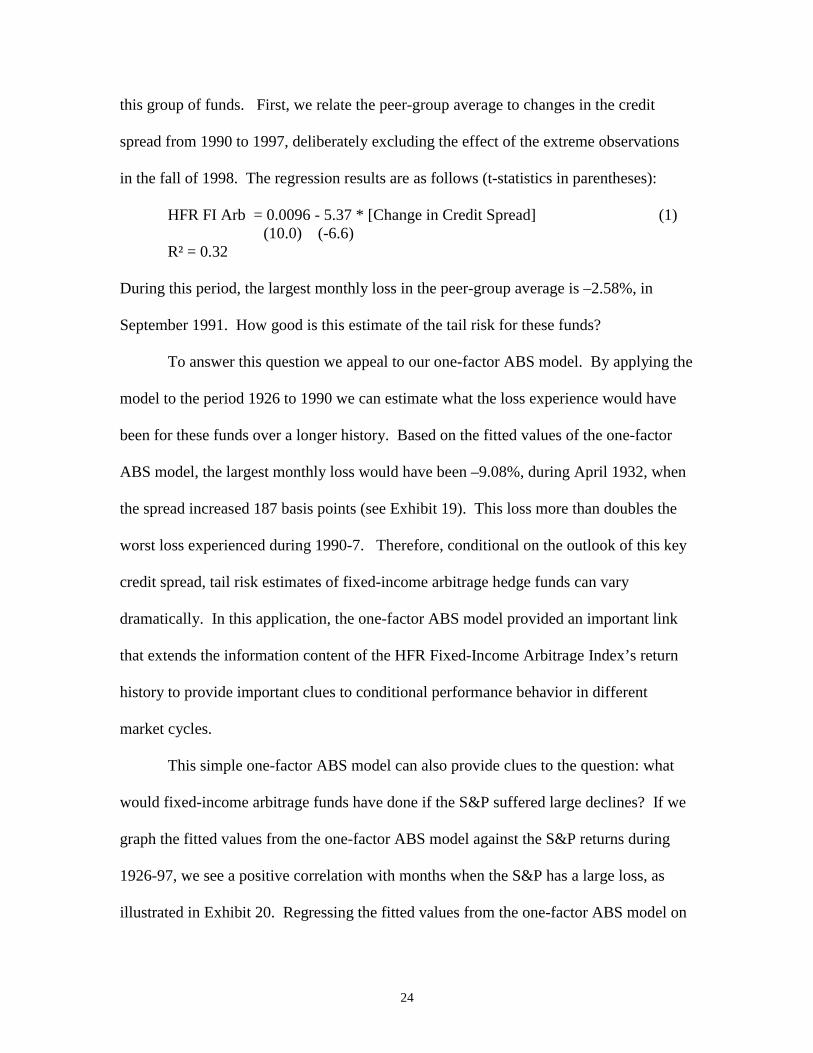
this group of funds. First, we relate the peer-group average to changes in the credit

spread from 1990 to 1997, deliberately excluding the effect of the extreme observations

in the fall of 1998. The regression results are as follows (t-statistics in parentheses):

HFR FI Arb = 0.0096 - 5.37 * [Change in Credit Spread] (1)(10.0) (-6.6)

R² = 0.32

During this period, the largest monthly loss in the peer-group average is –2.58%, in

September 1991. How good is this estimate of the tail risk for these funds?

To answer this question we appeal to our one-factor ABS model. By applying the

model to the period 1926 to 1990 we can estimate what the loss experience would have

been for these funds over a longer history. Based on the fitted values of the one-factor

ABS model, the largest monthly loss would have been –9.08%, during April 1932, when

the spread increased 187 basis points (see Exhibit 19). This loss more than doubles the

worst loss experienced during 1990-7. Therefore, conditional on the outlook of this key

credit spread, tail risk estimates of fixed-income arbitrage hedge funds can vary

dramatically. In this application, the one-factor ABS model provided an important link

that extends the information content of the HFR Fixed-Income Arbitrage Index’s return

history to provide important clues to conditional performance behavior in different

market cycles.

This simple one-factor ABS model can also provide clues to the question: what

would fixed-income arbitrage funds have done if the S&P suffered large declines? If we

graph the fitted values from the one-factor ABS model against the S&P returns during

1926-97, we see a positive correlation with months when the S&P has a large loss, as

illustrated in Exhibit 20. Regressing the fitted values from the one-factor ABS model on

25

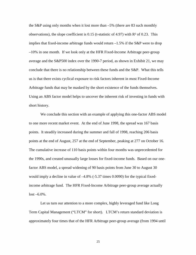
the S&P using only months when it lost more than –5% (there are 83 such monthly

observations), the slope coefficient is 0.15 (t-statistic of 4.97) with R² of 0.23. This

implies that fixed-income arbitrage funds would return –1.5% if the S&P were to drop

–10% in one month. If we look only at the HFR Fixed-Income Arbitrage peer-group

average and the S&P500 index over the 1990-7 period, as shown in Exhibit 21, we may

conclude that there is no relationship between these funds and the S&P. What this tells

us is that there exists cyclical exposure to risk factors inherent in most Fixed-Income

Arbitrage funds that may be masked by the short existence of the funds themselves.

Using an ABS factor model helps to uncover the inherent risk of investing in funds with

short history.

We conclude this section with an example of applying this one-factor ABS model

to one more recent market event. At the end of June 1998, the spread was 167 basis

points. It steadily increased during the summer and fall of 1998, reaching 206 basis

points at the end of August, 257 at the end of September, peaking at 277 on October 16.

The cumulative increase of 110 basis points within four months was unprecedented for

the 1990s, and created unusually large losses for fixed-income funds. Based on our one-

factor ABS model, a spread widening of 90 basis points from June 30 to August 30

would imply a decline in value of –4.8% (-5.37 times 0.0090) for the typical fixed-

income arbitrage fund. The HFR Fixed-Income Arbitrage peer-group average actually

lost –6.0%.

Let us turn our attention to a more complex, highly leveraged fund like Long

Term Capital Management (“LTCM” for short). LTCM’s return standard deviation is

approximately four times that of the HFR Arbitrage peer-group average (from 1994 until

26

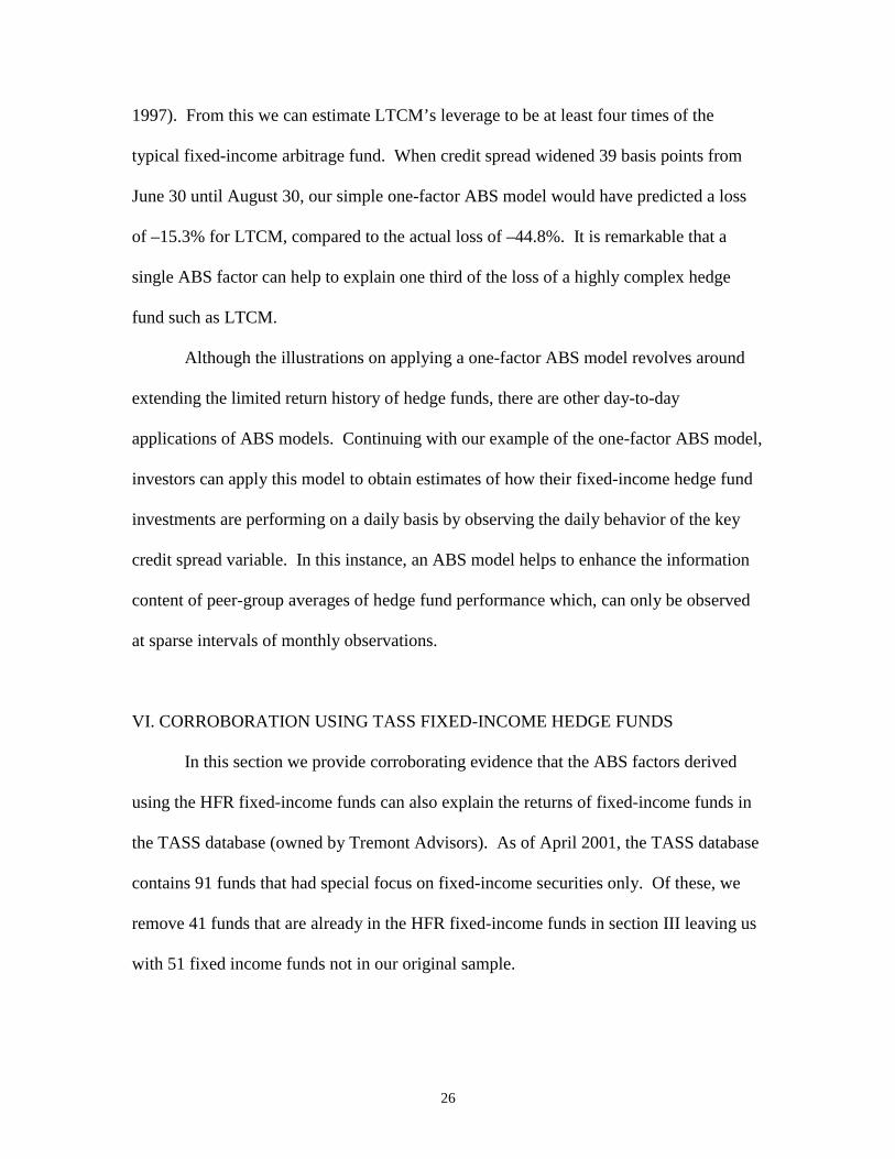
1997). From this we can estimate LTCM’s leverage to be at least four times of the

typical fixed-income arbitrage fund. When credit spread widened 39 basis points from

June 30 until August 30, our simple one-factor ABS model would have predicted a loss

of –15.3% for LTCM, compared to the actual loss of –44.8%. It is remarkable that a

single ABS factor can help to explain one third of the loss of a highly complex hedge

fund such as LTCM.

Although the illustrations on applying a one-factor ABS model revolves around

extending the limited return history of hedge funds, there are other day-to-day

applications of ABS models. Continuing with our example of the one-factor ABS model,

investors can apply this model to obtain estimates of how their fixed-income hedge fund

investments are performing on a daily basis by observing the daily behavior of the key

credit spread variable. In this instance, an ABS model helps to enhance the information

content of peer-group averages of hedge fund performance which, can only be observed

at sparse intervals of monthly observations.

VI. CORROBORATION USING TASS FIXED-INCOME HEDGE FUNDS

In this section we provide corroborating evidence that the ABS factors derived

using the HFR fixed-income funds can also explain the returns of fixed-income funds in

the TASS database (owned by Tremont Advisors). As of April 2001, the TASS database

contains 91 funds that had special focus on fixed-income securities only. Of these, we

remove 41 funds that are already in the HFR fixed-income funds in section III leaving us

with 51 fixed income funds not in our original sample.

27

A principal component analysis on these 51 funds reveals that the first three

components explained, respectively, 22%, 17%, and 15% of their cross-section variation.

They jointly account for more than 50% of the cross-section variation.

In terms of return-based style factors, the first component has a correlation of 0.88

with the first component of the HFR Diversified funds. The second component has a

correlation of 0.58 with the first component of the HFR Arbitrage funds. The third

component has a correlation of 0.70 with the HFR High-Yield funds.

In terms of ABS factors, the first component is strongly negatively correlated with

the 10-year lookback straddle on corporate bonds (R²=0.36), which is indicative of the

presence of convergence trading strategies. The second component is strongly negatively

correlated with the 10-year lookback straddle on mortgage spreads (R²=0.41) and is also

indicative of convergence trading strategies being used. The third component is strongly

positively correlated with the high-yield bonds-minus-treasury return (R²=0.52). This

may also be evidence of convergence trading, since the high-yield bonds-minus-treasury

return is highly negatively correlated with the 10-year lookback straddle on the high yield

spread (as discussed in Section III).

V. COMPARISON WITH FIXED-INCOME MUTUAL FUND STYLES

In this section we compare the styles of fixed-income hedge funds and fixed-

income mutual funds. From the Morningstar January 2002 CD-ROM, we extract mutual

funds from seven style categories that invest in similar fixed-income securities as the

HFR fixed-income hedge funds; see Exhibit 22 for details.

28

For each Morningstar category, we perform principal component analysis on all

the funds with data from 1998 to 2000 to determine the number of common styles.

Exhibit 23 gives the percent of cross-sectional variation explained by the first two

principal components in each category. It shows that each category has only one main

style. Furthermore, the first principal component of each category has high correlation

(the lowest being 0.985) with the average return of the mutual funds in that category.17

This allows us to use the average return to proxy for the return of that particular style.

Results from Sharpe’s [1992] style regressions on these mutual fund peer-group

averages are summarized in Exhibit 24. In four instances, only one benchmark is needed

to achieve high explanatory powers. In three other cases, two to three benchmarks are

needed. The lowest R² is 0.92.

Lastly, we add static spread factors (e.g. mortgage-minus-treasury returns) and

dynamic strategies (e.g. short- and long- horizon lookback straddles) to the style

regressions. None can replace or replicate the explanatory power of the standard

benchmarks in Exhibit 24. This evidence confirms the stylized fact that fixed-income

mutual funds styles have predominantly passive exposure to standard benchmarks.

VI. CONCLUSIONS

This paper analyzes the common risk of fixed-income hedge funds by extracting

seven return-based style factors, which are then linked them to ABS factors. Primarily,

fixed-income hedge funds have static exposure to fixed-income related spreads—they

are, respectively, convertible/treasury spread, high-yield/treasury spread,

mortgage/treasury spread, and emerging market bond/treasury spread. However, there is

29

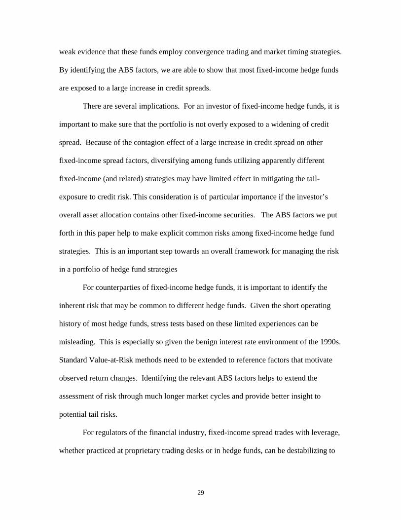
weak evidence that these funds employ convergence trading and market timing strategies.

By identifying the ABS factors, we are able to show that most fixed-income hedge funds

are exposed to a large increase in credit spreads.

There are several implications. For an investor of fixed-income hedge funds, it is

important to make sure that the portfolio is not overly exposed to a widening of credit

spread. Because of the contagion effect of a large increase in credit spread on other

fixed-income spread factors, diversifying among funds utilizing apparently different

fixed-income (and related) strategies may have limited effect in mitigating the tail-

exposure to credit risk. This consideration is of particular importance if the investor’s

overall asset allocation contains other fixed-income securities. The ABS factors we put

forth in this paper help to make explicit common risks among fixed-income hedge fund

strategies. This is an important step towards an overall framework for managing the risk

in a portfolio of hedge fund strategies

For counterparties of fixed-income hedge funds, it is important to identify the

inherent risk that may be common to different hedge funds. Given the short operating

history of most hedge funds, stress tests based on these limited experiences can be

misleading. This is especially so given the benign interest rate environment of the 1990s.

Standard Value-at-Risk methods need to be extended to reference factors that motivate

observed return changes. Identifying the relevant ABS factors helps to extend the

assessment of risk through much longer market cycles and provide better insight to

potential tail risks.

For regulators of the financial industry, fixed-income spread trades with leverage,

whether practiced at proprietary trading desks or in hedge funds, can be destabilizing to

30

markets when extreme events occur. This is exacerbated by the convergence of

“strategies” among market participants leading to similar risk exposures. The key

question is how to detect the risk of such convergences early. This is not an easy

question to answer. The path to a reasonable solution must begin with understanding the

underlying risk characteristics of the strategies in question. Here, ABS factors can help

by identifying seemingly different strategies that have common ABS factors. This in turn

helps to devise early warning indicators that are risk factor-based rather than specific-

position based.

Lastly, the ABS factors we have extracted help to explain where fixed-income

hedge funds can add value to investors’ portfolios. Note that in Section V, we showed

that dynamic ABS factors are absent from traditional (e.g. mutual fund) investment

vehicles. This is prima facie evidence that hedge fund strategies, through their exposure

to ABS factors, are exposed to alternative sources of risk. It follows that the returns for

bearing these alternative sources of risk offer investors an alternative source of income

from standard asset categories. The caveat is that exposure to these alternative risks

requires additional tools to manager the attendant tail risk. The challenge here is to

develop a complete model of ABS factors for hedge funds in general. An ABS factor

model that can be integrated into an overall asset allocation framework, and explicitly

identifies the hedge-fund alpha that managers bring over and above the common risks of

different styles.

31

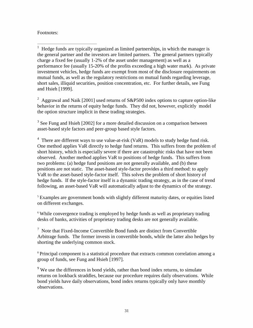
Footnotes:

1 Hedge funds are typically organized as limited partnerships, in which the manager isthe general partner and the investors are limited partners. The general partners typicallycharge a fixed fee (usually 1-2% of the asset under management) as well as aperformance fee (usually 15-20% of the profits exceeding a high water mark). As privateinvestment vehicles, hedge funds are exempt from most of the disclosure requirements onmutual funds, as well as the regulatory restrictions on mutual funds regarding leverage,short sales, illiquid securities, position concentration, etc. For further details, see Fungand Hsieh [1999].

2 Aggrawal and Naik [2001] used returns of S&P500 index options to capture option-likebehavior in the returns of equity hedge funds. They did not, however, explicitly modelthe option structure implicit in these trading strategies.

3 See Fung and Hsieh [2002] for a more detailed discussion on a comparison betweenasset-based style factors and peer-group based style factors.

4 There are different ways to use value-at-risk (VaR) models to study hedge fund risk.One method applies VaR directly to hedge fund returns. This suffers from the problem ofshort history, which is especially severe if there are catastrophic risks that have not beenobserved. Another method applies VaR to positions of hedge funds. This suffers fromtwo problems: (a) hedge fund positions are not generally available, and (b) thesepositions are not static. The asset-based style-factor provides a third method: to applyVaR to the asset-based style-factor itself. This solves the problem of short history ofhedge funds. If the style-factor itself is a dynamic trading strategy, as in the case of trendfollowing, an asset-based VaR will automatically adjust to the dynamics of the strategy.

5 Examples are government bonds with slightly different maturity dates, or equities listedon different exchanges.

6 While convergence trading is employed by hedge funds as well as proprietary tradingdesks of banks, activities of proprietary trading desks are not generally available.

7 Note that Fixed-Income Convertible Bond funds are distinct from ConvertibleArbitrage funds. The former invests in convertible bonds, while the latter also hedges byshorting the underlying common stock.

8 Principal component is a statistical procedure that extracts common correlation among agroup of funds, see Fung and Hsieh [1997].

9 We use the differences in bond yields, rather than bond index returns, to simulatereturns on lookback straddles, because our procedure requires daily observations. Whilebond yields have daily observations, bond index returns typically only have monthlyobservations.

32

10 To avoid dominance, one asset must have higher payoffs in some states of the worldand lower payoffs in some other states of the world.

11 The delta of the lookback straddle was calculated in Fung and Hsieh [2001].

12 We also try a 1-year lookback straddle. It does not materially alter the results of thepaper.

13 HFR’s style definitions are provided at the following website:https://www.hfr.com/hfram/index.php?action=moreInfo_monthlyIndices

14 These bond return indices include capital gains and coupon payments.

15 The correlation of HFR Fixed-Income Arbitrage peer-group average with the LehmanAggregate Bond index is –0.199.

16 Another way to see this is to extract principal components from the seven style factors.The first principal component explains 47% of the cross-sectional variation, while thesecond component explains only 26%. The first component is indeed credit risk, since ithas a correlation of -0.86 with the change in the high-yield credit spread.

17 There is survivorship bias in the Morningstar CD, since funds that ceased operationprior to December 2001 are excluded from the January 2002 CD. This would affect theestimate of mean return, but not the correlation with market benchmarks, given thehomogeneity of mutual fund returns within the same Morningstar category.

33

References:

Aggrawal, V., and N. Naik. "Characterizing the Risk and Return of Equity HedgeFunds." Working Paper, Georgia State University and London Business School, 2001.

Bank for International Settlements. "Banks’ Interactions with Highly LeveragedInstitutions." Basle Committee on Bank Supervision Publication No. 45, Basle, 1999a.

Bank for International Settlements. "Sound Practices for Banks’ Interactions with HighlyLeveraged Institutions." Basle Committee on Bank Supervision Publication No. 46,Basle, 1999b.

Bank for International Settlements. "A Review of Financial Market Events in Autumn1998." Committee on the Global Financial System Publication No. 12, Basle, 1999c.

Fung, W., and D.A. Hsieh. "Empirical Characteristics of Dynamic Trading Strategies:The Case of Hedge Funds." Review of Financial Studies, 10 (1997), pp. 275-302.

Fung, W., and D.A. Hsieh. "A Primer on Hedge Funds." Journal of Empirical Finance, 6(1999), pp. 309-331.

Fung, W., and D.A. Hsieh. "The Risk of Hedge Fund Strategies: Theory and Evidencefrom Trend Followers." Review of Financial Studies, 41 (2001), pp. 313-341.

Fung, W., and D.A. Hsieh. "Asset-Based Style Factors for Hedge Funds." FinancialAnalyst Journal, forthcoming (2002).

Goldman, M., H. Sosin, and M. Gatto. "Path Dependent Options: ’Buy at the Low, Sell atthe High’." Journal of Finance, 34 (1979), pp. 1111-1127.

Mitchell, M., and T. Pulvino. "Characteristics of Risk in Risk Arbitrage." Journal ofFinance, 56 (2001), pp. 2067-2109.

Perold, A. "Long-Term Capital Management, L.P." Harvard Business School, 9-200-007,1999.

President’s Working Group on Financial Markets. "Hedge Funds, Leverage, and theLessons of Long-Term Capital Management." Washington, D.C., 1999.

34

EXHIBIT 1HFR Fixed Income Indices, as of December 2000

Index Number AssetsCorrelation

to BondsHFR Fixed Income Convertible Bond 12 $1.5b 0.03HFR Fixed Income High-Yield Bond 20 $8.9b 0.09HFR Fixed Income Mortgage-Backed 17 $3.0b 0.11HFR Fixed Income Arbitrage 19 $4.4b -0.20HFR Fixed Income Diversified 39 $1.9b 0.51

Source: Hedge Fund Research.

35

EXHIBIT 2Percent of Cross-Sectional Variation Explained by Principal Components

% of Cross-Sectional VariationExplained

Index PC#1 PC#2 PC#3HFR Fixed Income Convertible Bond 59% 13%HFR Fixed Income High-Yield Bond 63% 16%HFR Fixed Income Mortgage-Backed 55% 17%HFR Fixed Income Arbitrage 33% 24% 16%HFR Fixed Income Diversified 36% 21% 11%

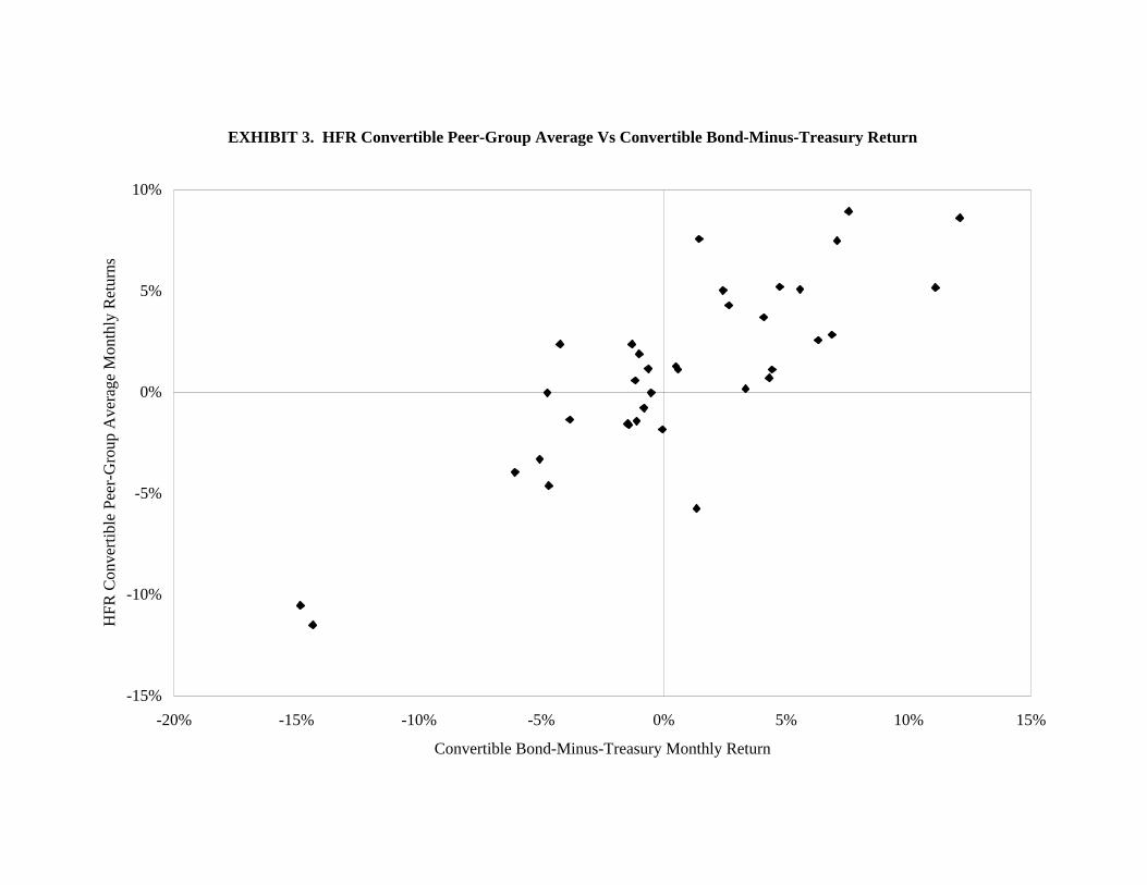
EXHIBIT 3. HFR Convertible Peer-Group Average Vs Convertible Bond-Minus-Treasury Return

-15%

-10%

-5%

0%

5%

10%

-20% -15% -10% -5% 0% 5% 10% 15%

Convertible Bond-Minus-Treasury Monthly Return

HFR

Con

vert

ible

Pee

r-G

roup

Ave

rage

Mon

thly

Ret

urns

EXHIBIT 4Summary of Regression Results on Hedge Fund Style Factors

DependentVariable Independent Variables Coeff T-stat F-test R²HFR Convertible Convertible-Treasury 0.673 9.0 81.2 0.70HFR High-Yield 10Y Lookback on HY -0.135 -11.3 128.3 0.79HFR Mortgage-Backed Change Mortgage Rate -20.88 3.2 15.3 0.59

Change Swap Rate 7.06 2.4Change 10y Rate 7.65 2.1

HFR Arbitrage PC#1 High Yield - Treasury 52.86 9.0 34.6 0.50HFR Arbitrage PC#2 Convertible-Treasury 15.68 3.7 18.1 0.35HFR Diversified PC#1 Corporate bond 158.1 4.6 21.2 0.38HFR Diversified PC#2 Emerging Mkt-Treasury -29.61 -9.2 85.1 0.71

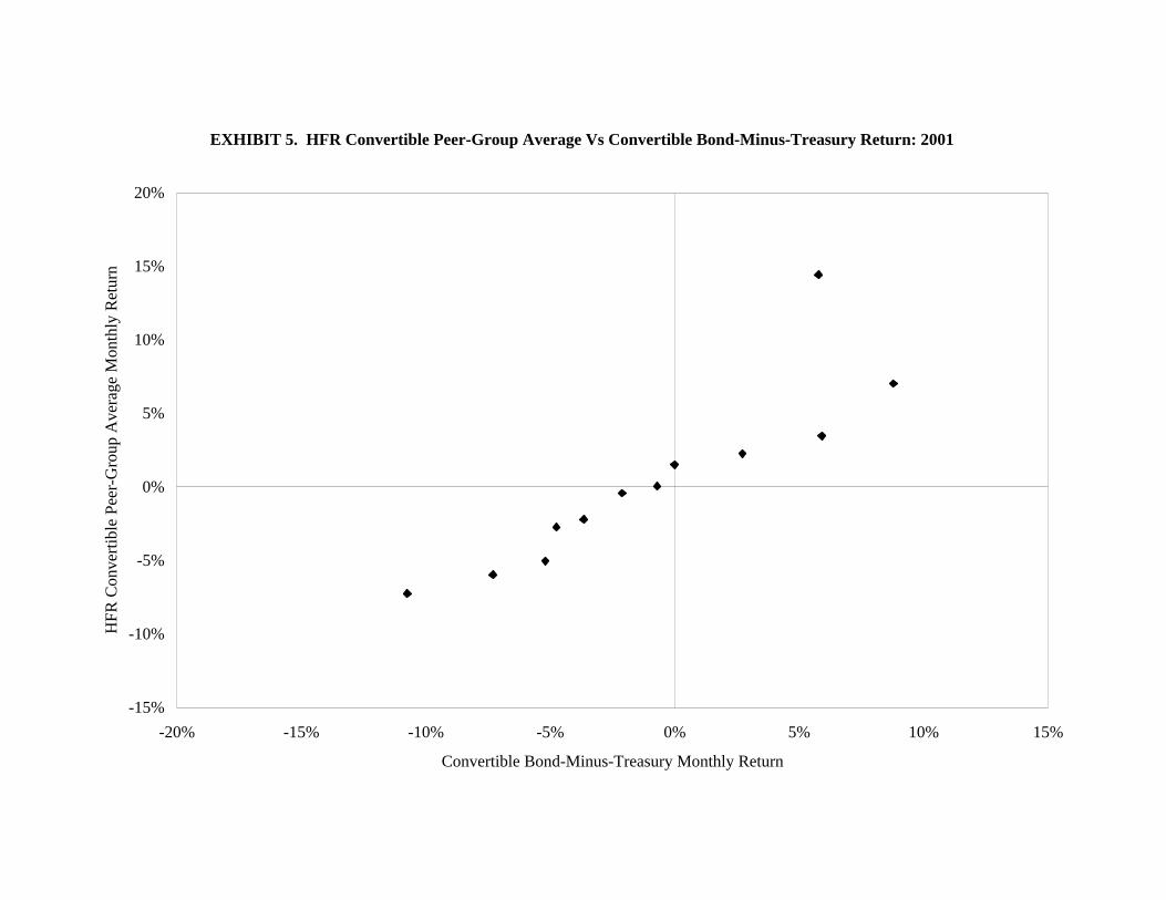
EXHIBIT 5. HFR Convertible Peer-Group Average Vs Convertible Bond-Minus-Treasury Return: 2001

-15%

-10%

-5%

0%

5%

10%

15%

20%

-20% -15% -10% -5% 0% 5% 10% 15%

Convertible Bond-Minus-Treasury Monthly Return

HFR

Con

vert

ible

Pee

r-G

roup

Ave

rage

Mon

thly

Ret

urn

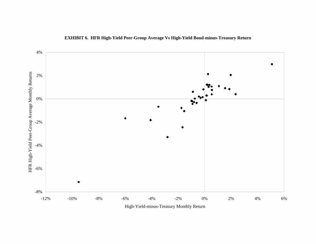
EXHIBIT 6. HFR High-Yield Peer-Group Average Vs High-Yield Bond-minus-Treasury Return

-8%

-6%

-4%

-2%

0%

2%

4%

-12% -10% -8% -6% -4% -2% 0% 2% 4% 6%

High-Yield-minus-Treasury Monthly Return

HFR

Hig

h-Y

ield

Pee

r-G

roup

Ave

rage

Mon

thly

Ret

urns

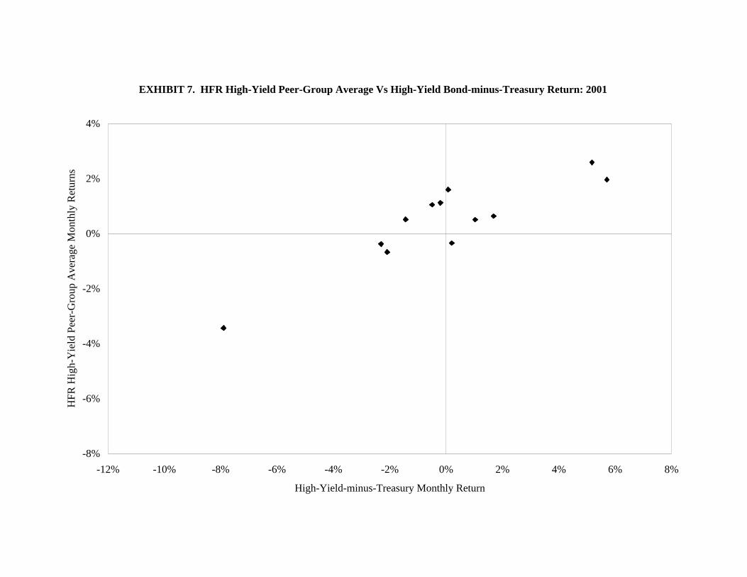
EXHIBIT 7. HFR High-Yield Peer-Group Average Vs High-Yield Bond-minus-Treasury Return: 2001

-8%

-6%

-4%

-2%

0%

2%

4%

-12% -10% -8% -6% -4% -2% 0% 2% 4% 6% 8%

High-Yield-minus-Treasury Monthly Return

HFR

Hig

h-Y

ield

Pee

r-G

roup

Ave

rage

Mon

thly

Ret

urns

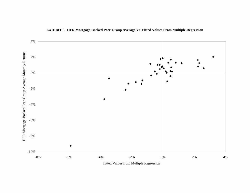
EXHIBIT 8. HFR Mortgage-Backed Peer-Group Average Vs Fitted Values From Multiple Regression

-10%

-8%

-6%

-4%

-2%

0%

2%

4%

-8% -6% -4% -2% 0% 2% 4%

Fitted Values from Multiple Regression

HFR

Mor

tgag

e-B

acke

d Pe

er-G

roup

Ave

rage

Mon

thly

Ret

urns

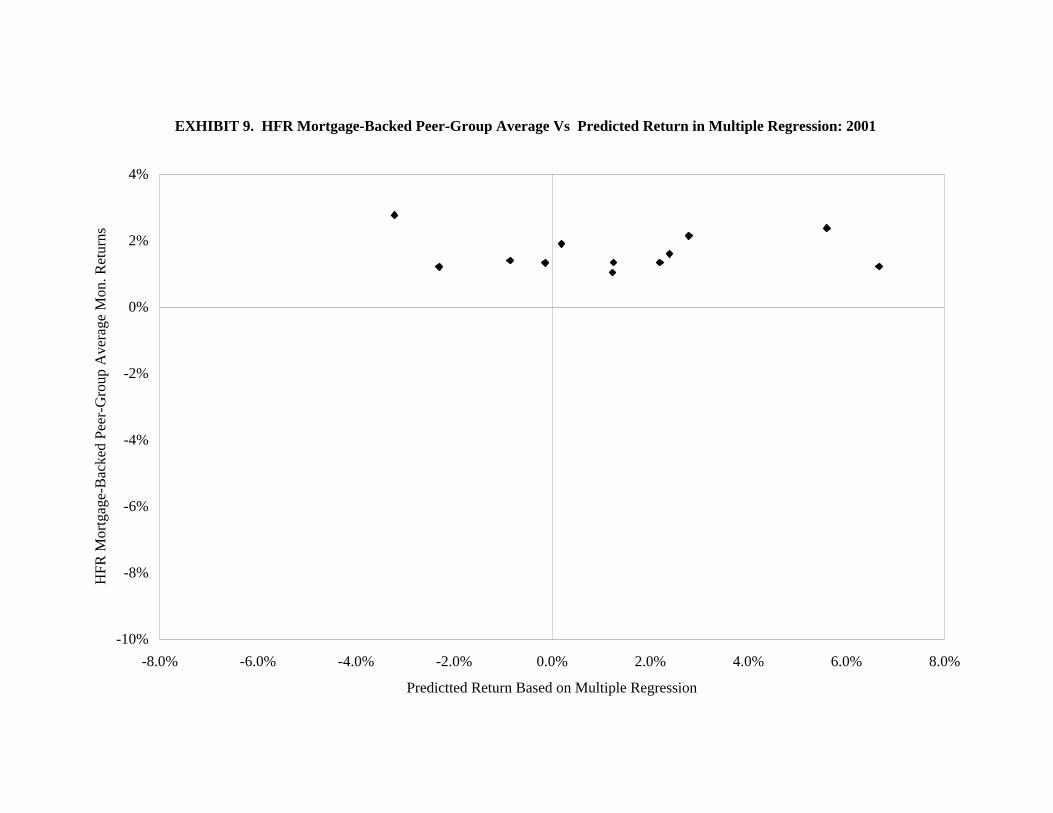
EXHIBIT 9. HFR Mortgage-Backed Peer-Group Average Vs Predicted Return in Multiple Regression: 2001

-10%

-8%

-6%

-4%

-2%

0%

2%

4%

-8.0% -6.0% -4.0% -2.0% 0.0% 2.0% 4.0% 6.0% 8.0%

Predictted Return Based on Multiple Regression

HFR

Mor

tgag

e-B

acke

d Pe

er-G

roup

Ave

rage

Mon

. Ret

urns

EXHIBIT 10. Arbitrage Funds’ First Principal Component Vs High-Yield Bond-Minus-Treasury

-6

-5

-4

-3

-2

-1

0

1

2

3

-12% -10% -8% -6% -4% -2% 0% 2% 4% 6%

High-Yield Bond-Minus-Treasury Monthly Return

Arb

itrag

e Fu

nd’s

Fir

st P

rinc

ipal

Com

pone

nt

EXHIBIT 11. Arbitrage Funds’ Second Principal Component Vs Convertible Bond-Minus-Treasury

-5

-4

-3

-2

-1

0

1

2

3

4

5

-20% -15% -10% -5% 0% 5% 10% 15%

Convertible Bond-Minus-Treasury Monthly Return

Arb

itrag

e Fu

nd’s

Sec

ond

Prin

cipa

l Com

pone

nt

EXHIBIT 12. HFR Arbitrage Peer-Group Average Vs Fitted Values

-8.0%

-6.0%

-4.0%

-2.0%

0.0%

2.0%

4.0%

-3.0% -2.5% -2.0% -1.5% -1.0% -0.5% 0.0% 0.5% 1.0% 1.5% 2.0%

Fitted Monthly Return Based On Principal Components

HFR

Arb

itrag

e Pe

er-G

roup

Ave

rage

Mon

thly

Ret

urn

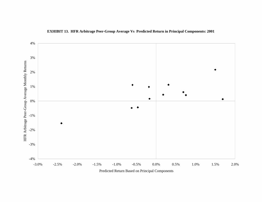
EXHIBIT 13. HFR Arbitrage Peer-Group Average Vs Predicted Return in Principal Components: 2001

-4%

-3%

-2%

-1%

0%

1%

2%

3%

4%

-3.0% -2.5% -2.0% -1.5% -1.0% -0.5% 0.0% 0.5% 1.0% 1.5% 2.0%

Predicted Return Based on Principal Components

HFR

Arb

itrag

e Pe

er-G

roup

Ave

rage

Mon

thly

Ret

urns

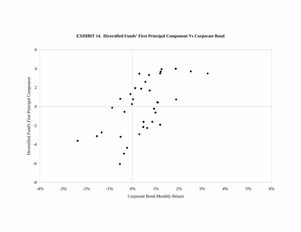
EXHIBIT 14. Diversified Funds’ First Principal Component Vs Corporate Bond

-8

-6

-4

-2

0

2

4

6

-4% -3% -2% -1% 0% 1% 2% 3% 4% 5% 6%

Corporate Bond Monthly Return

Div

ersi

fied

Fun

d’s

Firs

t Pri

ncip

al C

ompo

nent

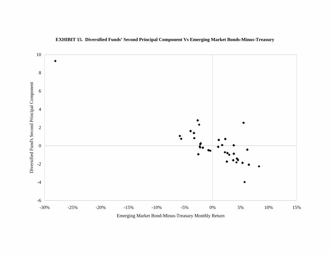
EXHIBIT 15. Diversified Funds’ Second Principal Component Vs Emerging Market Bonds-Minus-Treasury

-6

-4

-2

0

2

4

6

8

10

-30% -25% -20% -15% -10% -5% 0% 5% 10% 15%

Emerging Market Bond-Minus-Treasury Monthly Return

Div

ersi

fied

Fun

d’s

Seco

nd P

rinc

ipal

Com

pone

nt

EXHIBIT 16. HFR Diversified Peer-Group Average Vs Fitted Values

-2.0%

-1.0%

0.0%

1.0%

2.0%

3.0%

4.0%

5.0%

6.0%

-1.5% -1.0% -0.5% 0.0% 0.5% 1.0% 1.5% 2.0% 2.5%

Fitted Monthly Return Based on Principal Components

HFR

Div

ersi

fied

Pee

r-G

roup

Ave

rage

Mon

thly

Ret

urn

EXHIBIT 17. HFR Diversified Peer-Group Average Vs Predicted Return in Principal Components: 2001

-2%

-1%

0%

1%

2%

3%

4%

5%

6%

-1.5% -1.0% -0.5% 0.0% 0.5% 1.0% 1.5% 2.0% 2.5%

Predicted Return Based on Principal Components

HFR

Div

ersi

fied

Pee

r-G

roup

Ave

rage

Mon

thly

Ret

urns

EXHIBIT 18. HFR Fixed-Income Peer-Group Averages Vs Change in Credit Spread

-15%

-10%

-5%

0%

5%

10%

-0.40% -0.30% -0.20% -0.10% 0.00% 0.10% 0.20% 0.30% 0.40% 0.50% 0.60%Change in Credit Spread

HFR

Fix

ed-I

ncom

e Pe

er-G

roup

Ave

rage

s M

onth

ly R

etur

ns

Conv HY MBS Arb Div

EXHIBIT 19. Long Term History of the Credit Spread

0%

1%

2%

3%

4%

5%

6%

7%

8%

Dec

-24

Dec

-27

Dec

-30

Dec

-33

Dec

-36

Dec

-39

Dec

-42

Dec

-45

Dec

-48

Dec

-51

Dec

-54

Dec

-57

Dec

-60

Dec

-63

Dec

-66

Dec

-69

Dec

-72

Dec

-75

Dec

-78

Dec

-81

Dec

-84

Dec

-87

Dec

-90

Dec

-93

Dec

-96

Dec

-99

EXHIBIT 20. Predicted Arbitrage Peer-Group Average Monthly Returns vs S&P: 1926-1997

-15%

-10%

-5%

0%

5%

10%

15%

-40% -30% -20% -10% 0% 10% 20% 30% 40% 50%

S&P Monthly Returns

Pred

icte

d A

rbitr

age

Peer

-Gro

up A

vera

ge M

onth

ly R

etur

ns

EXHIBIT 21. HFR Arbitrage Peer-Group Average Vs S&P: 1990-97

-3%

-2%

-1%

0%

1%

2%

3%

4%

5%

6%

-40% -30% -20% -10% 0% 10% 20% 30% 40% 50%

S&P Monthly Returns

HFR

Arb

itrag

e Pe

er-G

roup

Ave

rage

Mon

thly

Ret

urns

EXHIBIT 22Morningstar Fixed Income Mutual Fund Styles: December 2001

Morningstar Style Category Number AssetsConvertible Securities 66 $ 7.7bEmerging Market Bonds 41 $ 3.0bHigh Yield Bonds 371 $ 82.1bInternational Bonds 137 $ 13.5bIntermediate Bonds 656 $215.3bIntermediate Government 302 $ 86.6bLong Term Bonds 96 $ 16.2b

Source: Morningstar January 2002 CD-ROM.

EXHIBIT 23Percent of Cross-Sectional Variation Explained by Principal Components

Morningstar Style Category PC#1 PC#2Convertible Securities 87% 5%Emerging Market Bonds 97% 1%High Yield Bonds 87% 3%International Bonds 63% 13%Intermediate Bonds 86% 6%Intermediate Government 89% 5%Long Term Bonds 77% 13%Long Term Governments 92% 4%

EXHIBIT 24Summary of Regression Results on Mutual Fund Style Factors

DependentVariable Independent Variables Coeff T-stat F-test R²Convertible Securities CSFB Convertible 0.82 22.6 509.3 0.94Emerging Market Bonds JPM Brady 1.16 27.6 71.6 0.96High Yield Bonds CSFB High Yield 1.10 37.0 1368.6 0.98International Bonds JPM World ExUS 0.41 15.9 155.7 0.94

JPM Brady 0.07 7.0Lehman Credit 0.24 5.9

Intermediate Bonds Lehman IT Credit 0.96 24.7 612.2 0.95Intermediate Government Lehman IT Gov 0.68 12.8 617.1 0.92

Lehman IT Mortgage 0.49 8.6Long Term Bonds Lehman LT Credit 0.45 8.8 164.5 0.94

Lehman LT Gov 0.09 2.2Lehman Mortgage 0.38 3.8

Long Term Governments Lehman LT Gov 0.65 34.2 1420.9 0.99Lehman Mortgage 0.35 7.1

Data Appendix

Series SourceCSFB Convertible Bond Index Morningstar CDCSFB High Yield Bond Index Morningstar CDLehman Aggregate Bond Total Return Index DatastreamLehman Credit Index DatastreamLehman Treasury Total Return Index DatastreamLehman Mortgage Backed Securities Total Return Index DatastreamJ.P. Morgan Non-US Government Bond DatastreamJ.P. Morgan Brady Broad Index Datastream