fractional polynomials and model averaging - stata · fractional polynomials and model averaging...
TRANSCRIPT

Fractional Polynomials and Model Averaging
Paul C LambertCenter for Biostatistics and Genetic Epidemiology
University of LeicesterUK
Nordic and Baltic Stata Users Group Meeting, Stockholm7th September 2007
Paul C Lambert Fractional Polynomials and Model Averaging Stockholm, 7th September 2007 1/28

Fractional Polynomials
Fractional Polynomials are used in regression models to fitnon-linear functions.
Often preferable to cut-points.
Functions from fractional polynomials more flexible than from‘standard’ polynomials.
See (Royston and Altman, 1994) or (Sauerbrei and Royston,1999) for more details.
Implemented in Stata with fracpoly and mfp commands.
Paul C Lambert Fractional Polynomials and Model Averaging Stockholm, 7th September 2007 2/28

Powers
The linear predictor for a fractional polynomial of order M forcovariate x can be defined as,
β0 +M∑
m=1
βmxpm
where each power pm is chosen from a restricted set.
The usual set of powers is
{−2,−1,−0.5, 0, 0.5, 1, 2, 3}
x0 is taken as ln(x)
Paul C Lambert Fractional Polynomials and Model Averaging Stockholm, 7th September 2007 3/28

Selecting the Best Fitting Model
All combinations of powers are fitted and the ’best’ fitting modelobtained.
Using the default set of powers for an FP2 model there are
8 FP1 Models36 FP2 Models (including 8 repeated powers)
The best fitting model for fractional polynomials of the samedegree can be obtain by minimising the deviance.
When comparing models of a different degree, e.g. FP2 and FP1models, the model can be selected using a formal significancetest or the Akaike Information Criterion (AIC).
Model selection uncertainty is ignored.
Paul C Lambert Fractional Polynomials and Model Averaging Stockholm, 7th September 2007 4/28

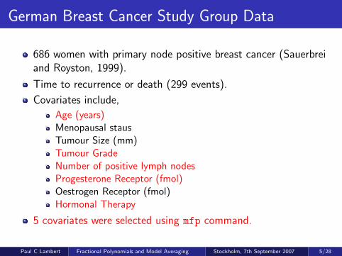
German Breast Cancer Study Group Data
686 women with primary node positive breast cancer (Sauerbreiand Royston, 1999).
Time to recurrence or death (299 events).
Covariates include,
Age (years)Menopausal stausTumour Size (mm)Tumour GradeNumber of positive lymph nodesProgesterone Receptor (fmol)Oestrogen Receptor (fmol)Hormonal Therapy
5 covariates were selected using mfp command.
Paul C Lambert Fractional Polynomials and Model Averaging Stockholm, 7th September 2007 5/28

Breast Cancer - Best Fitting Model for Age
−1
0
1
2
3
4
5
Log
Haz
ard
Rat
io
20 40 60 80age, years
Best Fitting Model (−2 −.5), AIC = 3562.73
Paul C Lambert Fractional Polynomials and Model Averaging Stockholm, 7th September 2007 6/28

Breast Cancer - Best Fitting Model for Age
−1
0
1
2
3
4
5
Log
Haz
ard
Rat
io
20 40 60 80age, years
Best Fitting Model (−2 −.5), AIC = 3562.73
FP2(-2 -0.5): ln(h(t)) = ln(h0(t)) + β1Age−2∗ + β2Age−0.5
∗Paul C Lambert Fractional Polynomials and Model Averaging Stockholm, 7th September 2007 6/28
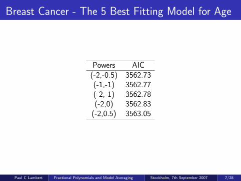
Breast Cancer - The 5 Best Fitting Model for Age
Powers AIC(-2,-0.5) 3562.73(-1,-1) 3562.77(-2,-1) 3562.78(-2,0) 3562.83
(-2,0.5) 3563.05
Paul C Lambert Fractional Polynomials and Model Averaging Stockholm, 7th September 2007 7/28

Breast Cancer - Age
−1
0
1
2
3
4
5
Log
Haz
ard
Rat
io
20 40 60 80age, years
Best Fitting Model (−2 −.5), AIC = 3562.73
Paul C Lambert Fractional Polynomials and Model Averaging Stockholm, 7th September 2007 8/28

Breast Cancer - Age
−1
0
1
2
3
4
5
Log
Haz
ard
Rat
io
20 40 60 80age, years
Powers (−1 −1), AIC = 3562.77
Paul C Lambert Fractional Polynomials and Model Averaging Stockholm, 7th September 2007 8/28

Breast Cancer - Age
−1
0
1
2
3
4
5
Log
Haz
ard
Rat
io
20 40 60 80age, years
Powers (−2 −1), AIC = 3562.78
Paul C Lambert Fractional Polynomials and Model Averaging Stockholm, 7th September 2007 8/28

Breast Cancer - Age
−1
0
1
2
3
4
5
Log
Haz
ard
Rat
io
20 40 60 80age, years
Powers (−2 0), AIC = 3562.83
Paul C Lambert Fractional Polynomials and Model Averaging Stockholm, 7th September 2007 8/28

Breast Cancer - Age
−1
0
1
2
3
4
5
Log
Haz
ard
Rat
io
20 40 60 80age, years
Powers (−2 .5), AIC = 3563.05
Paul C Lambert Fractional Polynomials and Model Averaging Stockholm, 7th September 2007 8/28

Breast Cancer - No. Positive Lymph Nodes
−7
−5
−3
−1
1
3
Log
Haz
ard
Rat
io
0 5 10 15 20 25 30 35 40 45 50 55number of positive nodes
Best Fitting Model (1 2), AIC = 3498.99
Paul C Lambert Fractional Polynomials and Model Averaging Stockholm, 7th September 2007 9/28
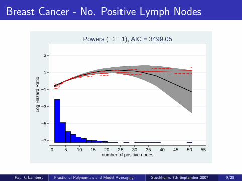
Breast Cancer - No. Positive Lymph Nodes
−7
−5
−3
−1
1
3
Log
Haz
ard
Rat
io
0 5 10 15 20 25 30 35 40 45 50 55number of positive nodes
Powers (−1 −1), AIC = 3499.05
Paul C Lambert Fractional Polynomials and Model Averaging Stockholm, 7th September 2007 9/28

Breast Cancer - No. Positive Lymph Nodes
−7
−5
−3
−1
1
3
Log
Haz
ard
Rat
io
0 5 10 15 20 25 30 35 40 45 50 55number of positive nodes
Powers (−2 −.5), AIC = 3499.12
Paul C Lambert Fractional Polynomials and Model Averaging Stockholm, 7th September 2007 9/28

Breast Cancer - No. Positive Lymph Nodes
−7
−5
−3
−1
1
3
Log
Haz
ard
Rat
io
0 5 10 15 20 25 30 35 40 45 50 55number of positive nodes
Powers (−2 −1), AIC = 3499.44
Paul C Lambert Fractional Polynomials and Model Averaging Stockholm, 7th September 2007 9/28

Breast Cancer - No. Positive Lymph Nodes
−7
−5
−3
−1
1
3
Log
Haz
ard
Rat
io
0 5 10 15 20 25 30 35 40 45 50 55number of positive nodes
Powers (1 3), AIC = 3499.64
Paul C Lambert Fractional Polynomials and Model Averaging Stockholm, 7th September 2007 9/28

Model Averaging 1
In FP models the model selection process is usually ignored whencalculating fitted values and their associated confidence intervals.
Model Averaging is popular Bayesian research area (Hoetinget al., 1999), (Congdon, 2007).
Increasing interest from frequentist perspective (Burnham andAnderson, 2004) (Buckland et al., 2007) (Congdon, 2007) (Faeset al., 2007)
Usually interest lies in model averaging for a parameter.
Here we are interested in averaging over the functional formobtained from different models.
Paul C Lambert Fractional Polynomials and Model Averaging Stockholm, 7th September 2007 10/28

Model Averaging 2
If there are K contending models, Mk , k = 1, . . . ,K withweights, wk , which are scaled so that
∑wk = 1, then the
estimate of a parameter or quantity, θ (assumed to be commonto all models) is taken to be,
θa =K∑
k=1
wk θk
The variance of θa is,
var(θa
)=
K∑k=1
w 2k
(var(θk |Mk
)+(θk − θa
)2)
Paul C Lambert Fractional Polynomials and Model Averaging Stockholm, 7th September 2007 11/28

Obtaining the Weights, wk
In a Bayesian context we want, wk = P(Mk |Data)
These probabilities are not trivial to calculate and variousapproximations are available.
One such approximation is to use the Bayesian InformationCriterion (BIC)
BICk = ln(Lk)− 1
2p ln(n)
The AIC can also be used to derive the model weights (Bucklandet al., 2007)
AICk = ln(Lk)− 2p
Recently Faes used the AIC to derive model weights forfractional polynomial models (Faes et al., 2007).
Paul C Lambert Fractional Polynomials and Model Averaging Stockholm, 7th September 2007 12/28

Obtaining the Weights, wk
Let
∆k = BICk − BICmin or ∆k = AICk − AICmin
The weights, wk , are then defined as,
wk =exp(
12∆k
)∑Kj=1 exp
(12∆j
)
Paul C Lambert Fractional Polynomials and Model Averaging Stockholm, 7th September 2007 13/28

Using Bootstrapping to Obtain the Weights, wk
An alternative to using the AIC or BIC for the model weights,wk , is to use bootstrapping (Hollander et al., 2006).
For each bootstrap sample the best fitting fractional polynomialmodel is selected.
The weights wk , are simply obtained using the frequencies of themodels selected over the B bootstrap samples.
If comparing fractional polynomial models of different degreesthen some selection process is needed. This is usually done bysetting a value for α.
Paul C Lambert Fractional Polynomials and Model Averaging Stockholm, 7th September 2007 14/28

Using fpma
Using fpma.
. fpma x1, ic(aic) xpredict: stcox x1Models Included (in order of weight)
Powers AIC deltaAIC weight cum. weight
1 -2 -.5 3562.73 0.00 0.0802 0.08022 -1 -1 3562.77 0.03 0.0789 0.15913 -2 -1 3562.78 0.04 0.0785 0.23764 -2 0 3562.83 0.09 0.0766 0.31425 -2 .5 3563.05 0.31 0.0686 0.38276 -1 -.5 3563.05 0.32 0.0685 0.45127 -2 -2 3563.26 0.53 0.0616 0.51288 -2 1 3563.38 0.65 0.0580 0.57099 -1 0 3563.50 0.77 0.0546 0.6255
10 -.5 -.5 3563.52 0.79 0.0540 0.6795
(output omitted )43 2 3578.18 15.44 0.0000 1.000044 3 3578.32 15.58 0.0000 1.0000
New variables created xb ma xb ma se xb ma lci xb ma uci
Paul C Lambert Fractional Polynomials and Model Averaging Stockholm, 7th September 2007 15/28

Using fpma - Bootstrapping (α = 0.05)
Using fpma with bootstrapping.
. fpma x1, ic(bootstrap) xpredict xpredname(x1_ma_boot1) reps(1000): stcox x1Running 1000 bootstrap samples to determine model weights(bootstrap: maboot)
Powers Freq. weight cum. weight
1 -2 -2 252 0.2520 0.25202 -2 -1 167 0.1670 0.41903 -1 -1 163 0.1630 0.58204 -1 -.5 88 0.0880 0.67005 1 71 0.0710 0.74106 -2 67 0.0670 0.80807 -.5 -.5 63 0.0630 0.87108 -2 -.5 51 0.0510 0.92209 -.5 0 30 0.0300 0.9520
10 0 0 19 0.0190 0.971011 0 .5 6 0.0060 0.9770
(output omitted )22 -1 0 1 0.0010 0.999023 -.5 .5 1 0.0010 1.0000
Paul C Lambert Fractional Polynomials and Model Averaging Stockholm, 7th September 2007 16/28

Breast Cancer - Age
−1
0
1
2
3
4
5
Log
Haz
ard
Rat
io
20 40 60 80age, years
Model Average − BIC
Paul C Lambert Fractional Polynomials and Model Averaging Stockholm, 7th September 2007 17/28

Breast Cancer - Age
−1
0
1
2
3
4
5
Log
Haz
ard
Rat
io
20 40 60 80age, years
Model Average − AIC
Paul C Lambert Fractional Polynomials and Model Averaging Stockholm, 7th September 2007 17/28

Breast Cancer - Age
−1
0
1
2
3
4
5
Log
Haz
ard
Rat
io
20 40 60 80age, years
Model Average − Bootstrap (alpha = 0.05)
Paul C Lambert Fractional Polynomials and Model Averaging Stockholm, 7th September 2007 17/28
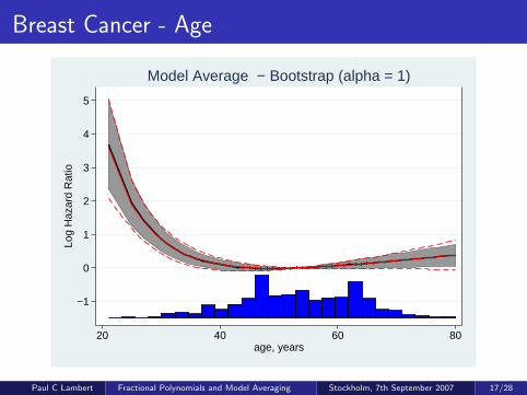
Breast Cancer - Age
−1
0
1
2
3
4
5
Log
Haz
ard
Rat
io
20 40 60 80age, years
Model Average − Bootstrap (alpha = 1)
Paul C Lambert Fractional Polynomials and Model Averaging Stockholm, 7th September 2007 17/28

Breast Cancer - No. of Positive Lymph Nodes
−7
−5
−3
−1
1
3
Log
Haz
ard
Rat
io
0 5 10 15 20 25 30 35 40 45 50 55number of positive nodes
Model Average − BIC
Paul C Lambert Fractional Polynomials and Model Averaging Stockholm, 7th September 2007 18/28

Breast Cancer - No. of Positive Lymph Nodes
−7
−5
−3
−1
1
3
Log
Haz
ard
Rat
io
0 5 10 15 20 25 30 35 40 45 50 55number of positive nodes
Model Average − AIC
Paul C Lambert Fractional Polynomials and Model Averaging Stockholm, 7th September 2007 18/28

Breast Cancer - No. of Positive Lymph Nodes
−7
−5
−3
−1
1
3
Log
Haz
ard
Rat
io
0 5 10 15 20 25 30 35 40 45 50 55number of positive nodes
Model Average − Bootstrap (alpha = 0.05)
Paul C Lambert Fractional Polynomials and Model Averaging Stockholm, 7th September 2007 18/28

Breast Cancer - No. of Positive Lymph Nodes
−7
−5
−3
−1
1
3
Log
Haz
ard
Rat
io
0 5 10 15 20 25 30 35 40 45 50 55number of positive nodes
Model Average − Bootstrap (alpha = 1)
Paul C Lambert Fractional Polynomials and Model Averaging Stockholm, 7th September 2007 18/28

Breast Cancer - No. of Positive Lymph Nodes¡20
−2
−1.5
−1
−.5
0
.5
1
1.5
2
Log
Haz
ard
Rat
io
0 5 10 15 20number of positive nodes
Model Average − BIC
Paul C Lambert Fractional Polynomials and Model Averaging Stockholm, 7th September 2007 19/28

Breast Cancer - No. of Positive Lymph Nodes¡20
−2
−1.5
−1
−.5
0
.5
1
1.5
2
Log
Haz
ard
Rat
io
0 5 10 15 20number of positive nodes
Model Average − AIC
Paul C Lambert Fractional Polynomials and Model Averaging Stockholm, 7th September 2007 19/28
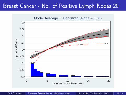
Breast Cancer - No. of Positive Lymph Nodes¡20
−2
−1.5
−1
−.5
0
.5
1
1.5
2
Log
Haz
ard
Rat
io
0 5 10 15 20number of positive nodes
Model Average − Bootstrap (alpha = 0.05)
Paul C Lambert Fractional Polynomials and Model Averaging Stockholm, 7th September 2007 19/28

Breast Cancer - No. of Positive Lymph Nodes¡20
−2
−1.5
−1
−.5
0
.5
1
1.5
2
Log
Haz
ard
Rat
io
0 5 10 15 20number of positive nodes
Model Average − Bootstrap (alpha = 1)
Paul C Lambert Fractional Polynomials and Model Averaging Stockholm, 7th September 2007 19/28

Multivariable Fractional Polynomials
The above only really applies when using fractional polynomialsfor only one of the covariates in the model.
However, is is common to use models with fractionalpolynomials for more than one covariate.
A simple approach is to model average over various fractionalpolynomial models for the covariate of interest, while keepingthe functional form of the remaining covariates constant.
The usemfp option will do this for you.
Paul C Lambert Fractional Polynomials and Model Averaging Stockholm, 7th September 2007 20/28

Using mfp with Model Averaging
mfp.
. mfp stcox x1 x2 x3 x4a x4b x5 x6 x7 hormon, nohr alpha(.05) select(0.05)(output omitted )
Final multivariable fractional polynomial model for _t
Variable Initial Finaldf Select Alpha Status df Powers
x1 4 0.0500 0.0500 in 4 -2 -.5x2 1 0.0500 0.0500 out 0x3 4 0.0500 0.0500 out 0
x4a 1 0.0500 0.0500 in 1 1x4b 1 0.0500 0.0500 out 0x5 4 0.0500 0.0500 in 4 -2 -1x6 4 0.0500 0.0500 in 2 .5x7 4 0.0500 0.0500 out 0
hormon 1 0.0500 0.0500 in 1 1
Cox regression -- Breslow method for ties(output omitted )
Paul C Lambert Fractional Polynomials and Model Averaging Stockholm, 7th September 2007 21/28
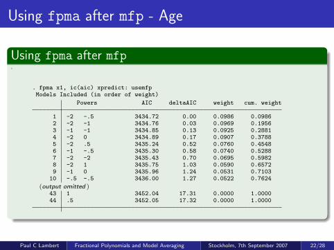
Using fpma after mfp - Age
Using fpma after mfp.
. fpma x1, ic(aic) xpredict: usemfpModels Included (in order of weight)
Powers AIC deltaAIC weight cum. weight
1 -2 -.5 3434.72 0.00 0.0986 0.09862 -2 -1 3434.76 0.03 0.0969 0.19563 -1 -1 3434.85 0.13 0.0925 0.28814 -2 0 3434.89 0.17 0.0907 0.37885 -2 .5 3435.24 0.52 0.0760 0.45486 -1 -.5 3435.30 0.58 0.0740 0.52887 -2 -2 3435.43 0.70 0.0695 0.59828 -2 1 3435.75 1.03 0.0590 0.65729 -1 0 3435.96 1.24 0.0531 0.7103
10 -.5 -.5 3436.00 1.27 0.0522 0.7624
(output omitted )43 1 3452.04 17.31 0.0000 1.000044 .5 3452.05 17.32 0.0000 1.0000
Paul C Lambert Fractional Polynomials and Model Averaging Stockholm, 7th September 2007 22/28

Model Averaging after mfp - Age
−1
0
1
2
3
4
5
Log
Haz
ard
Rat
io
20 40 60 80age, years
AIC weights
Paul C Lambert Fractional Polynomials and Model Averaging Stockholm, 7th September 2007 23/28

Model Averaging after mfp - No. of Positive Lymph Nodes
−7
−5
−3
−1
1
3
Log
Haz
ard
Rat
io
0 5 10 15 20 25 30 35 40 45 50 55number of positive nodes
AIC weights
Paul C Lambert Fractional Polynomials and Model Averaging Stockholm, 7th September 2007 24/28

Discussion
Fractional Polynomials very useful for modelling non-linearfunctions.
Model selection uncertainty is usually ignored after final model isobtained.
Model averaging is easy to implement and incorporates FPmodel selection uncertainty.
Still further work needed. For example,
Statistical properties (coverage etc).Comparison with fully Bayesian model averaging.
Paul C Lambert Fractional Polynomials and Model Averaging Stockholm, 7th September 2007 25/28

References I
Buckland, S., Burnham, K., and Augustin, N. (2007). Model selection: An intergral part of inference. Biometrics,53(2):603–618.
Burnham, K. P. and Anderson, D. R. (2004). Multimodal inference: Understanding AIC and BIC in model selection.Sociological Methods and Research, 33(2):261–304.
Congdon, P. (2007). Model weights for model choice and averaging. Statistical Methodology, 4:143–157.
Faes, C., Aerts, M., H., G., and Molenberghs, G. (2007). Model averaging using fractional polynomials to estimate a safe levelof exposure. Risk Analysis, 27(1):111–123.
Hoeting, J. A., Madigan, D., E., R. A., and Volinsky, C. T. (1999). Bayesian model averaging: A tutorial. Statistical Science,14(4):382–417.
Hollander, N., Augustin, N., and Sauerbrei, W. (2006). Investigation on the improvement of prediction by bootstrap modelaveraging. Methods of Information in Medicine, 45:44–50.
Royston, P. and Altman, D. (1994). Regression using fractional polynomials of continuous covariates: parsimonious parametricmodelling. JRSSA, 43(3):429–467.
Sauerbrei, W. and Royston, P. (1999). Building multivariable prognostic and diagnostic models: transformation of thepredictors by using fractional polynomials. JRSSA, 162(1):71–94.