Froms: A Failure Tolerant and MobilityEnabled Multicast Routing Paradigm with

Reinforcement Learning for WSNs

ANNA FORSTERUniversity of Lugano, Swizterland

andAMY L. MURPHY

FBK-IRST, Trento, Italy

University of LuganoFaculty of Informatics

Technical Report No. 2009/004June 2009

Abstract

A growing class of wireless sensor network (WSN) applications re-quire the use of sensed data inside the network at multiple, possiblymobile base stations. Standard WSN routing techniques that movedata from multiple sources to a single, fixed base station are not ap-plicable, motivating new solutions that efficiently achieve multicast.This paper explores in depth the requirements of this set of applicationscenarios and proposes, Froms, a machine learning-based approach.The primary benefits are the flexibility to optimize routing on a varietyof properties such as route length, battery levels, etc., ease of recoveryafter node failures, and native support for sink mobility. We provideextensive simulation results supporting these claims, clearly showingthe benefits of Froms in terms of low routing overhead, extendednetwork lifetimes, and other key metrics for the WSN environment.

1

1 Introduction

The 1998 SmartDust [1] project is commonly used to mark the beginningof wireless sensor network (WSNs) research, as it identified the vision forlarge autonomous networks for monitoring environmental and industrial pa-rameters. Since then the price of individual sensors has been decreasing,while memory, processing and sensory abilities have been increasing, simul-taneously expanding the potential application scenarios. Researchers andpractitioners from many scientific and industrial areas have already lever-aged the achievements of the WSN community, deploying of sensor networkswith applications ranging from scientific monitoring of active volcanos [2]and glaciers [3], through agricultural monitoring [4], military and rescueapplications[5, 6], to the futuristic vision of the InterPlaNetary Internet [7, 8],designed to connect highly heterogeneous devices such as satellites, Mars andMoon rovers, sensor networks, space shuttles, and common handheld devicesand laptops into one holistic network.

The growing number of applications for WSNs and especially their het-erogeneous requirements and properties demand new communication proto-cols and architectures. Routing for WSNs has attracted a lot of research inrecent years, and many different protocols has been developed for variousapplication scenarios and data traffic schedules. However, lately this areahas attracted extensive criticism: application scenarios are too restricted ornot carefully described, experimental setups are unrealistic, and simulationenvironments are too abstract [9]. Further, despite the overwhelming numberand variety of routing protocols, key problems remain unsolved, importantlyenergy efficiency in various application scenarios and for multiple traffic pat-terns, and tolerance against failures and mobility has not been sufficientlyaddressed. Additionally, the problem of sending data to multiple, possiblymobile sinks via optimal paths (multicast) has not been solved efficiently.

This paper presents a novel multicast routing protocol called Froms(Feedback ROuting to Multiple Sinks), which exploits reinforcement learn-ing. Our target scenario includes any applications with periodic or long-lasting sensory data reporting to multiple, mobile sinks in a multi-hop envi-ronment. Froms easily accepts different cost metrics such as hops, latency,remaining battery etc.. Its most salient advantages are: the ability to findglobally optimal multicast routes; to incorporate different cost metrics andthus optimization goals; and to quickly recover in case of failures and sinkmobility. The main goal of Froms is to provide the WSN developer with one

2

routing solution, able to be tuned to many different application scenarios.This paper presents a comprehensive view of Froms, including a theoret-

ical model and an analysis of its complexity and overall behavior; a completeevaluation both in simulation and on real hardware; and a challenging com-parison against geographic based multicast routing protocol MSTEAM [10]and a multicast variation of Directed Diffusion [11]. The presented simulationenvironment uses sophisticated radio propagation models and realistic MACprotocols. In contrast to our previously reported results [12, 13], this paperoffers significantly more depth to the characterization of the Froms param-eter space and its properties, and a complete comparison to other multicastrouting protocols both in simulation and on real hardware.

Next, Section 2 motivates the work and our approach, describing majorchallenges and related works. Section 3 gives an intuitive introduction tothe Froms routing protocol, before Section 4 models multicast routing as areinforcement learning problem and presents our solution. Section 5 makesa theoretical complexity and convergence analysis. Section 6 proceeds withdefining the Froms protocol and discussing implementation details, beforeSections 7 – 10 present our evaluation environment and discuss the simula-tion and testbed experiments. Finally, Section 11 outlines future researchdirections and challenges.

2 Motivation and related efforts

In the next paragraphs we concentrate on the requirements and propertiesof well-known various WSN deployments and use them for defining our owntarget application scenario. Then we discuss the current state of the art ofWSN routing protocols and how they meet the needs and challenges of ouridentified scenario.

2.1 Target application scenario

Real deployments of wireless sensor networks usually implement one of threegeneral applications: periodic reporting, event detection [14], and data-baselike storage [15]. Periodic reporting is by far the most used and simplestapplication scenario: at regular intervals the sensors sample the environment,store the sensed data, and send it further to the base station(s). Actuators areoften directly connected with those sensor networks, for example automatic

3

irrigation systems or alarm systems.In this work we consider periodic reporting scenarios, since they make up

the major part of current and future WSN deployments. The main propertyof periodic reporting applications is the predictability of the data traffic andvolume. More precisely, we consider wireless sensor network applications todisaster relief and military operations [5, 6], environmental monitoring andsurveillance [2, 16, 17, 4, 18] and the InterPlaNetary Internet [7, 8]. Althoughthese scenarios are very different in their nature and goals, they share a lot ofproperties. In the next paragraphs we derive the properties of the applicationscenario for our routing protocol.

1. Network size. The sample WSN deployments we use in this work span awide variety of network sizes and densities. Some of them are randomlydeployed with hundreds of nodes (e.g. military or disaster recoveryapplications [5, 6]), others are thoroughly planned and include onlyfew to a dozen of nodes (volcano monitoring [2]).

Thus, we conclude that the number of nodes is unknown and can varyfrom only several nodes to hundreds or even thousands randomly or-ganized into a multi-hop topology.

2. Energy restrictions. One of the main challenges of wireless sensor net-works are the highly restricted power reserves of the sensor nodes. Theytypically have on-board low capacity batteries, which are used for sens-ing, processing and communication. However, the primary power con-sumer is the radio [19, 20], which drains the node’s battery quicklyfor active listening of the wireless medium and data transmission. Inaddition, many WSN deployments need to run unattended over weeksor even months and batteries cannot be replaced. This is the case,for example, for disaster relief operations [5] or for sensor networks aspart of the InterPlaNetary Internet [7, 8]. On the other hand, failingof some sensor nodes might disconnect the network and stop data de-livery. This event is often referred to as network death. Thus, one ofthe major design goals and requirements for data dissemination proto-cols is the efficient use of energy reserves and network life prolongationthrough on-board optimization and node-wide balancing of communi-cation overhead.

3. Node failures. Node failures are a direct consequence of the limitedenergy availability on the nodes. With dwindling battery reserves, the

4

node’s behavior becomes first very unreliable in terms of communica-tion and then the node fails completely. In unattended environmentsthe node will never recover. However, in agricultural monitoring [4, 18]exchange of batteries is possible and the node will re-enter the network.Node failure or restart can happen also for other reasons, for examplebecause of loose contacts, defect hardware or bad environmental con-ditions. A data dissemination framework needs to cope well with allthese events and to guarantee continuous data delivery during the fullnetwork lifetime. It also needs to accommodate new nodes to makeefficient use of all network resources.

4. Sink mobility. Sensor nodes in all our sample applications are usuallysimple, static entities. Current deployments often plan only one fixedbase station. However, this approach has various drawbacks: the basestation is a single point of failure and other data consumers in the sensornetwork have to retrieve the data directly from the base station. Thesecond argument is often considered an inconvenience rather than areal risk. However, imagine a disaster relief scenario as described in [6],where a sensor network has been deployed to observe the environment,estimate risks and discover people. The rescue workers are equippedwith wireless handheld devices, which usually are able to communi-cate with the base station (the emergency habitat). In the “normal”situation they can get sensory data from it directly. However, whathappens when they move around and their handheld devices go outof range of the base station? Usually no functioning infrastructure isavailable to ensure communication. In such cases the sensor networkitself can take over the communication among the sensor network, thebase station and the rescue workers. The consequence for data dis-semination protocols is that multiple mobile sinks are present in thenetwork.

Nearly the same situation arises in the InterPlaNetary Internet [7, 8].For environmental monitoring the need of mobile sinks is not that ur-gent, but it would be helpful to unobtrusively replace the base stationin case of failure or to receive the data directly from the sensor networkin case the used device has no access to the base station.

Thus, the routing protocol needs to support mobile sinks and to be ableto route data between heterogenous devices considering non-uniform

5

costs of the links.

5. Data generation, delivery and traffic. Usually there are many differentdata types available in a sensor network, e.g. temperature, humidity,light, gas concentration, acceleration. Sinks need to be able to choosebetween different data types, data sensing intervals, reporting intervals,compression parameters, etc. The sensing and reporting can be con-tinuos or temporary. The achievable throughput of a network dependsmostly on the Medium ACcess (MAC) protocol in use. The contribu-tion of the data dissemination protocols to managing data traffic is togenerate as few packets as possible. This lowers the overall latency,and increases the delivery rate and reliability. At the same time, sinks’requirements on data quality need to be met (see next point).

We assume that a suitable MAC protocol is used and the volume ofdata traffic can be anything between few readings from a single nodeto a single sink to all nodes reporting to several sinks.

6. Quality of service requirements. In addition to the data requirementsabove, the sinks have also quality of service requirements. Differentapplications have different requirements. For example, disaster reliefoperations [5] need reliable minimum delay delivery of sensory datafor ensuring fast response. In contrast, agricultural monitoring [4] is adelay-tolerant application where efficient energy use and long networklifetimes are more important to keep maintenance effort and costs low.

In summary, the designed routing protocol needs not only to supportall of these quality of services requirements, but to be able to switchbetween them quickly and efficiently. The most important requirementsare support of minimum delay, minimum energy expenditure, and highreliability (delivery rate).

Additionally, there are some important design criteria concerning thequality and the credibility of the conducted work. Unlike the requirementsoutlined above, which arise directly from the described deployments andapplications, the design criteria and their fulfillment are important for prac-titioners in the area and other researchers. They guarantee the real worldapplicability of the implemented routing protocol.

• Simplicity. The protocols must be easy to understand and implement,in order to be feasible for real-world deployments.

6

• Memory and processing requirements. The implementation must fitcomfortably onto a typical sensor node, leaving space for other proto-cols and applications.

• Flexibility. The protocol must be easily adaptable to different applica-tions and optimization goals.

• Scalability. The implemented protocols must be scalable in terms ofnetwork size, number of sources, and number of sinks.

In order to design and implement the routing protocol, we need to makesome assumptions about the rest of the communication stack:

1. Sink announcements (data requests). We assume that sinks announcethemselves via a network-wide broadcast in which they state their op-timization goal and data requirements. During this announcement, thenodes in the network are able to gather some initial routing informa-tion and to calculate in a localized manner their cluster membership.Propagating sink announcements is a very common approach in WSNs.

2. MAC layer. Routing protocols rely heavily on the lower layer protocols’performance. We consider a simple broadcast-enabled MAC protocolwithout re-transmissions and without delivery guarantee, basically anysensor network MAC protocol.

3. Neighborhood management. We do not assume any neighborhood man-agement protocol - the neighbors’ reliability and quality needs to bemanaged by the routing and clustering protocols directly, in order tobe able to manage failures and mobility in an efficient and holistic way.

This section presented and analyzed the most important application re-quirements for this work. In summary, our routing protocol needs to copewith different network sizes, multiple mobile sinks, failing nodes, restrictedenergy reserves, and various data and quality of service requirements.

Our first intuition is that machine learning seems a good choice for solvingthe above problems in an autonomous, self-organized, and energy-efficientway. In the next Section 2.2 we will explore related efforts on multicastrouting for WSN and machine learning approaches for routing in WSNs.

7

2.2 Application scenario challenges and related works

While a large body of different routing protocols [5] has emerged in the lastyears, there is still no general and well-performing routing protocol for WSNs.Real deployments often decide for a simple, already implemented routingprotocol based on hops like MintRoute [21] for TinyOS. However, they oftenalso change the protocol according to their needs [16, 4, 2], for example byusing a different neighborhood management protocol or a custom cost metric.Thus, the resulting protocols are highly specialized and optimized solutionsfor the targeted network rather than a standard protocol for a broad varietyof scenarios.

Multicast routing for WSNs. Many routing protocols have emergedfrom routing protocols for Mobile Ad Hoc Networks (MANETs). They builda full routing path table at all nodes and each node keeps the full routeto each possible destination. The main disadvantage of such an approachis that route information needs to be propagated throughout the network(from the source to the destination and back). Second, a complicated routerepair procedure needs to be started in case of topology changes or failures tore-build the routes. There are specialized multicast routing MANET rout-ing protocols, like MAODV [22], LAM [23], and ADMR [24]. Mesh-basedrouting protocols are a popular solution to multicast routing too, for exam-ple ODMPR [25] and PUMA [26]. They proved to be very efficient in highmobility scenarios, but cause great communication overhead for constructingand maintaining the mesh and thus cannot be successfully applied to WSNs.Such experiences were reported by various researchers while implementingMANET routing protocols for WSNs, like the implementation of ADMR onMicaZ motes [27]. There are some recent works using swarm intelligence [28](see the next section), but again the overhead from sending ants is unbearablefor wireless sensor networks.

Location-based (or geographic) network routing is based on the location-awareness of the nodes. Traditional geographic routing protocol is GPSR [29],which selects next hops based on their progress to the destination. In casethe routing is stuck (a node is reached with no progress to the sink), aspecial face routing procedure is started to route the packet around the voidregion. GMR [30] and MSTEAM [10] are both geographic based multicastrouting protocols. The main disadvantage of geographic routing protocols isthe length of the selected routes, especially in case of void regions. Another

8

problem with traditional geographic routing schemes is their preference oflong unreliable hops. In case no separate link protocol is used, geographicrouting selects next hops only based on their progress to the sink - thus,mostly long lossy connections. An extensive study of this problem and acomparison of various other location-based metrics on simulation and realhardware is presented in [31].

Another approach for WSNs for multicasting is what we call “fake mul-ticast”: unicast protocols, which are slightly optimized for multicast rout-ing. Such protocols just build paths from a source to each of the sinkswithout really considering sharing of paths or finding globally optimal ones.For example, Directed Diffusion [11] is a very popular and powerful routingparadigm, where routes from the source to the destinations are establishedon-demand based on interests that are flooded through the network. Thisflooding establishes gradients for data to follow from multiple sources to thesinks. It can be easily extended to multiple sinks, but the resulting multi-cast routes are not optimal. Nevertheless, Directed Diffusion has inspired alot of other routing protocols for WSNs, like Rumor routing [32] or GRE-DD [33]. MintRoute [21] from TinyOS1 is very similar to Directed Diffusion,but includes also a neighborhood management protocol.

Sink mobility management in WSNs. Some routing protocols as-sume that the mobility pattern of the sinks is known a-priori at the sensornodes. One such protocol is the spatiotemporal mobicast routing algorithmin [34]. This protocol is rather an overlay routing protocol, which decideswhen to forward the data through a geographic routing protocol to whichneighbors. In this way it guarantees spatiotemporal delivery of needed datato needed regions.

TTDD [35] is a layered routing protocol, developed especially for highmobility scenarios. The authors concentrate on efficient delivery to multiplemobile sinks through building a routing overlay. The network is clusteredinto cells and mobile sinks flood their requests in the local cell only. Thus, theoverlay is always aware of the current position of the sinks and routes the datato them. This approach proved to be very effective in high mobility scenarios.However, the nodes building the overlay (a cell structure) drain their powerquickly and the overlay has to be rebuilt with high communication overhead.Thats why the protocol is better suited for event-detecting sensor networks

1www.tinyos.org

9

with only sporadic traffic rather than continuous monitoring.SEAD [36] and its successor DEED [37] optimize routing from single

source to multiple mobile sinks. Each sink selects an “access sensor node”,to which data from the source is routed. A tree is built based on a geographiclocation heuristic between the source and all access nodes. When the sinkmoves away, a path between its current nearest neighbor and the access nodeis maintained, so that it is not necessary to rebuild the tree. If the sink movestoo far away, a new access node is selected and the tree is rebuilt, but onlywith high communication overhead. The approach shows very good resultscompared to Directed Diffusion [11] or TTDD [35] in terms of dissipatedenergy for data packets. However, no extensive evaluation of the controloverhead under mobile sinks is presented, which is expected to be high. Ananalytical evaluation of virtual infrastructure routing protocols (TTDD [35],SEAD [36] and others) is presented in [38].

2.3 Machine Learning applications to routing in WSNs

Machine learning has gained a lot of attention in latest years for solvinghard problems in wireless ad hoc networks such as routing [39, 40, 41]. InWSNs, reinforcement learning (RL) has been already applied to point-to-point routing in different settings - to support geographic routing [42]; fordiscovering routes between two nodes [43], for finding optimal compressionroutes between many sources and one sink [44] etc. All of these works showthe great advantage of using ML techniques for routing. However, to thebest of our knowledge, there are no works on applying machine learning(especially RL) to multicast routing, which requires changes to the originalML algorithms, while keeping their advantageous properties.

Another well known machine learning algorithm for routing is swarm in-telligence and especially ant colony optimization. It has been applied torouting in ad hoc networks in AntHocNet [28] and for point to point rout-ing in WSNs, but with less success. The main challenge is overcoming thecommunication overhead caused by the traveling ants. These algorithms arewell suited for highly mobile, energy-rich domains like MANETs and less forenergy-restricted, but rather static environments like WSNs.

10

P E A

BFH

CQ

S

Gsource

sink

sink

Neighbor A

routing table : node S

sink P 3 hopssink Q 5 hops

Neighbor B sink P 4 hopssink Q 4 hops

Neighbor C sink P 5 hopssink Q 3 hops

Figure 1: A sample topology with 2 sinks, the main routes to them fromsource S and its initial routing table.

3 Protocol intuition and overview

The goal of our protocol is to find the optimal possible path for data tofollow from its source to all interested sinks. Optimal can be defined aseither minimum delay, minimum hop count, minimum geographic distance,maximum remaining batteries or a combination of some of the above. Here,we will use number of hops as an example.

Consider the sample network from Figure 1 with one source and twosinks. One possible path from the source to the sinks is formed by the unionof the individual paths from the source to each sink (the dotted lines in thefigure), however a shorter path often exists. This shorter path takes theform of a tree, as the one through nodes B, F and H. The challenge is toglobally identify this tree without full topology information and using onlylocal information exchange. The main task of our protocol is to update localinformation regarding “next-hops” to reach sinks from each node such thatthe cost of the resulting tree is optimal.

During an initial sink announcement phase, as proposed in Section 2.1,all nodes gather some initial routing information and register known sinks inthe network. In our example from Figure 1 node S gathers hop informationfor each sink individually as shown in its routing table in the figure. Whendata packets arrive at the node for routing, the node needs to select one ormore next hops towards the sinks. However, instead of simply choosing thebest looking one (in this example: node C for sink Q and node A for sinkP ), it also explores non-optimal routes in the assumption that some of themmight have lower costs than in its own routing table. This is because itsneighboring nodes may be able to share next hops too. For example, thesource node S estimates that node A needs 7 hops to reach both sinks: 5hops to sink P , 3 hops to sink Q and the first hop is shared, thus the minus

11

1 or a total of 7 hops. However, node S does not know whether node A willbe able also to share the next hop or will need to split the packet and sendit through two different neighbors. In our example, node A is in fact able toshare the next hop. It calculates that it can reach the sinks through node E(see the routing table of node A in the figure) in (2 + 4)− 1 = 5 hops. Thus,node S will be able to reach both sinks in 1 hop to node A plus 5 hops fromnode A to all sinks or a total of 6 hops, which is 1 hop less than the initialinformation on the source node. Thus, node A needs to inform node S aboutits own estimation of the costs to both sinks. It can do so while sending thedata packet further to the sink by making use of the broadcast environmentand piggybacking its own cost estimation.

Similarly, node E piggybacks its cost estimation and informs node A andso on. There are four important observations to make: these piggybackedvalues, which we also call feedbacks, propagate exactly one step back untilthey reach the sinks, where the packet stops. Thus, the source needs to sendseveral data packets to node A before its own cost estimation for node Arepresents the real hop cost of the route.

Second, the source needs to send data packets not only to node A, butto all neighboring nodes a sufficient number of times, before all of its costestimations converge. The neighbors of the nodes need to also explore theirneighbors and so on. Third, feedback can be used not only by the previoushop, but by all overhearing nodes of the transmitter and thus deliver ad-ditional information to the nodes. And fourth, keeping all of the routes atall nodes and always giving feedback to the neighbors with the current costestimations, innately handles recovery and mobility. For example, in casenode E fails, node A will switch to another route, for example through nodeB, will update its cost estimations and will inform the source S via feedbackon the next data packet about its current costs. The information propagatestogether with the data packets, without incurring any additional communi-cation overhead and update automatically the routes and their costs on allinvolved nodes.

The above made observations form a reinforcement learning based rout-ing protocol. In the next section we formalize the ideas discussed here andpresent the details of the Q-Learning model, solving the multicast problemin WSNs.

12

4 FROMS: Solving Multicast with Q-Learning

The main goal of this section is to model the multicast routing problem andsolve it with reinforcement learning, as sketched in the pervious section. Thiswill not only build the basis of our protocol, but also give us the possibility tomake a theoretical analysis of the protocol in terms of complexity, correctnessand convergence.

4.1 Problem definition

We consider the network of sensors as a graph G = (V,E) where each sensornode is a vertex vi and each edge eij is a bidirectional wireless communicationchannel between a pair of nodes vi and vj. Without a loss of generality, weconsider a single source node s ∈ V and a set of destination nodes D ⊆ V .

Optimal routing to multiple destinations is defined as the minimum costpath starting at the source vertex s, and reaching all destination vertices D.This path is actually a spanning tree T = (VT , ET ) whose vertexes includethe source and the destinations. The cost of a tree T is defined as a functionover its nodes and links C(T ). For example, it can be the number of one-hopbroadcasts required to reach all destinations or in other words the number ofnon-leaf nodes in T . Further cost functions are presented in Section 6.8 andevaluated in Section 9.3.

4.2 Multicast Routing with Q-Learning

Finding the minimum cost tree T , also called the Steiner tree, is NP-hard,even when the full topology is known [45]. Our goal, therefore, is to approx-imate the optimal solution using localized techniques. We turn to reinforce-ment learning and especially to Q-Learning [46].

In our multiple-sink scenario, each sensor node is an independent learningagent, and actions are routing options using different neighbor(s) for the nexthop(s) toward a subset of the sinks, Dp ⊆ D, listed in the data packet. Themain challenge in our application is to model the actions of the nodes, sincethey contain not a single next hop (route to some neighbor n), but a-prioriunknown number of next hops. The following provides additional detail forthe Q-Learning solution.

Agent states. We define the state of an agent as a tuple {Dp, routesNDp},

13

whereDp ⊆ D are the sinks the packet must reach and routesNDp

is the routinginformation about all neighboring nodes N with respect to the individualsinks. Depending on this state, different actions are possible.

Actions. In our model, an action is one possible routing decision for adata packet. However, the routing decision can include one or more differentneighbors as next hops. Consequently, we need to change the original Q-Learning algorithm and define a possible action, a, as a set of sub-actions{a1 . . . ak}. Each sub-action ai = (ni, Di) includes a single neighbor ni and aset of destinations Di ⊆ Dp indicating that neighbor ni is the intended nexthop for routing to destinations Di. A complete action is a set of sub-actionssuch that {D1 . . . Dk} partitions Dp (that is, each sink d ∈ Dp is covered byexactly one sub-action ai).

Continuing with our example from Figure 1, consider a packet destined forDp = {P,Q}. One possible complete action of the source S is the single sub-action (B, {P,Q}), indicating neighbor B as the next hop to all destinations.Alternately, node S may choose two sub-actions, (A, {P}) and (C, {Q}),indicating two different neighbors should take responsibility to forward thepacket to different subsets of sinks.

The distinction between complete actions and sub-actions is important,as we assign rewards to sub-actions.

Q-Values. Q-Values represent the goodness of actions and the goal ofthe agent is to learn the actual goodness of the available actions. Here wediffer from the original Q-Learning, which randomly initializes Q-Values, andwhere Q-Values serve only for quantitative comparison.

In our case, we bound the Q-Values to represent the real cost of the routes,for example, if the cost function is number of hops, the Q-Value of a routeis also the number of hops of this route. To initialize these values, we use amore sophisticated approach than random assignment, which calculates anestimate of the cost based on the individual information about the involvedneighbor and sinks. This non-random initialization significantly speeds upthe learning process and avoids oscillations of the Q-Values.

For example, without loss of generality and continuing our example with ahop-based cost function, it estimates the route cost by using the hop countsavailable in a standard routing table, such as that in Figure 1. We firstcalculate the value of a sub-action, then of a complete action. The initialQ-Value for a sub-action ai = (ni, Di) is thus:

14

Q(ai) =

(∑d∈Di

hopsnid

)− 2(| Di | −1) (1)

where hopsnid are the number of hops to reach destination d ∈ Di using

neighbor ni and | Di | is the number of sinks in Di. The first part of theformula calculates the total number of hops to individually reach the sinks,and the second part subtracts from this total based on the assumption thatbroadcast communication is used both (hence the 2) for transmission to ni

as well as by ni to reach the next hop. Note that this estimation is an upperbound of the actual value, as it assumes that the packet will not share anylinks after the next hop. Therefore, during learning, Q-Values will alwaysdecrease and the best actions will be denoted with small Q-Values.

The Q-Value of a complete action a with sub-actions {a1, . . . , ak} is:

Q(a) =

( ∑ai∈a,i=1...k

Q(ai)

)− (k − 1) (2)

where k is the number of sub-actions. Intuitively this Q-Value is thebroadcast hop count from the agent to all sinks.

The above is an example of calculating the Q-Values when using thespecific hop-based cost. We will explore further cost metrics in Section 6.8.

Updating a Q-Value. To learn the real values of the actions, the agentmust receive the reward values from the environment. In our case, eachneighbor to which a data packet is forwarded sends the reward as feedbackwith its evaluation of the goodness of the sub-action. The new Q-Value ofthe sub-action is:

Qnew(ai) = Qold(ai) + γ(R(ai)−Qold(ai)) (3)

where R(ai) is the reward value and γ is the learning rate of the algorithm.We use γ = 1 to speed up learning. Usually a lower learning rate needs to beused with randomly initialized Q-Values, since otherwise they will oscillateheavily in the beginning of the learning process. However, since our valuesare guaranteed to decrease and not to oscillate, we can avoid the learningrate and the resulting delay in learning. Therefore, with γ = 1, the formulabecomes

15

Qnew(ai) = R(ai) (4)

directly updating the Q-Value with the reward. The Q-Values of completeactions are updated automatically, since their calculation is based on sub-actions (Equation 2).

Reward function. Intuitively the reward is the downstream node’s op-portunity to inform the upstream neighbors of its actual cost for the requestedaction. Thus, when calculating the reward, the node selects its lowest (best)Q-Value for the destination set and adds the cost of the action itself:

R(ai) = cai+ min

aQ(a) (5)

where caiis the action’s cost (always 1 in our hop count metric). This

propagation of Q-Values upstream eventually allows all nodes to learn theactual costs.

In contrast to the original Q-Learning algorithm, low reward values aregood and large values are bad. This is because we define the Q-Values torepresent the real hop costs of some route and thus the lowest Q-Values arethe best. Furthermore, rewards from the environment are generated and sentout without real knowledge of who receives them. Note also that the rewardvalues are completely localized and simply indicate the current best Q-Valueat the rewarding node.

Exploration strategy (action selection policy). One final, impor-tant learning parameter is the action selection policy. A trivial solution isto greedily select the action with the best (lowest) Q-Value. However, thispolicy ignores some actions which may, after learning, have lower Q-Values,resulting in a locally optimal solution. Therefore, a tradeoff is required be-tween exploitation of good routes and exploration among available routes. Asimple, though efficient strategy is ε-greedy, which selects the best availableaction with probability 1− ε and a random one with probability ε. There arealso variants of ε-greedy, where ε is decreased with time or where the rangeof random routes are restricted to the most promising ones. Section 6.9 givesmore details about the exploration strategies we use for Froms.

16

Parameter Description

D number of destinations

M diameter of the network

Y network density (maximum number of 1-hop neighbors)

|N | number of nodes in the network

A Maximum number of possible actions at each node

S Maximum number of action steps (sent packets) at thesource before convergence

Table 1: Summary of network scenario and complexity parameters, as usedin the discussion of Froms.

5 Theoretical analysis of FROMS

In this section we concentrate on the theoretical analysis of Froms: onits convergence, complexity, memory, and processing requirements. First weexplore an idealized model of the environment and later we introduce realisticproperties like asymmetric links and link failures.

5.1 Worst-case complexity and convergence

We show first the worst-case complexity of Froms (time to stabilize) andthus also implicitly its convergence. In our scenario, convergence means thatfirst, the protocol is stable and the Q-Values do not change any more, andsecond and more importantly, that the optimal route has been identified. Theoriginal Q-Learning algorithm has been shown to converge after an infinitenumber of steps [46]. Here we need to show that our Q-Learning basedprotocol converges after a finite number of steps. For this, we start bycalculating the number of steps until convergence.

First, we assume a Q-Learning algorithm like the one we presented inthe previous Section 4 with γ = 1, hop-based cost metric, and deterministicexploration strategy, which chooses the routes in a round-robin manner. Wefurther assume a network N with the following properties: D is the number ofdestinations, M is the diameter of the network (the longest shortest path inthe network between any two nodes in N) and Y is the density of the network(the maximum number of 1-hop neighbors at any node inN). The parameters

17

are summarized in Table 1. We also assume static nodes and sinks andperfect communication between the neighbors. Without loss of generality,we assume a single source, since the routes are constructed depending on thedestinations, not on the sources. We will discuss multiple sources at the endof this section.

Further, the maximum number of possible actions A at any node is, ac-cording to the definition of actions in Section 4, the number of permutationsof size D over all neighbors Y with repetitions (because we are allowed touse the same neighbor to reach multiple sinks) or:

A ≤ Y D (6)

In the worst case the source of the data or the initiator of the learningprocess is at maximum distance M from all of the sinks. Our goal is tocompute how many action selection steps have to be taken on all nodes inN , so that the Q-Values stabilize. With γ = 1 the feedback of any 1-hopneighbor is used for direct replacement of the old Q-Value. Thus, in order tolearn the real costs of any route of length M we need exactly M − 1 steps.However, the source has to first wait for all other nodes to stabilize theirQ-Values before it can be guaranteed that its Q-Values are stable too. Inthe worst case it has to explore the full network and all possible routes in it.Let us count the number of action selection steps S we need for the wholesystem to converge.

Assuming the learning is always initiated by the source, we know that weneed to select each of the routes available M − 1 times. Using Equation 6we have:

S ≤ (M − 1) · Y D

The 1-hop neighbors of the source need to do the same. Their distanceto the sinks is also at most M . Note this is the worst case and it actuallycannot exist in a real network: if all of the neighbors of some node are at thesame distance from the sinks as the node itself, the network is disconnected.Thus, all of the nodes in the network have to select each of their routes atmost M times. Thus, we have for the complexity:

S ≤ (M − 1) · |N | · Y D = O((M − 1) · |N | · Y D

)(7)

This is the worst-case number of actions across all nodes (packet broad-casts) for the protocol to converge. After convergence, exploration can be

18

stopped and the algorithm can proceed in a greedy mode, as the best routehas been identified and has the best Q-Value among all available. If thereare more than one best routes, they can be alternated to spread energy ex-penditure.

However, this is a very loose upper bound of the complexity - no realnetworks have the worst-case properties like ”all neighbors are M hops awayfrom the destinations”. However, it gives us an idea about the scalabilityof the approach and its expected performance. In the next paragraphs wediscuss in detail how the convergence behavior changes with various networkparameters and what are the consequences for the protocol. We use experi-mental evaluations to show the real behavior of the protocol in Sections 4-9.

Parameter analysis. The number of destinations D and the density Yare not directly dependent on the number of nodes |N | in a network or onthe diameter M . To understand better the expected performance, we explorethese individual cases for each of the parameters:

The number of sinks D is completely independent from any of the othernetwork properties, |N |, M , or Y , as it is a requirement of the application.The only limitation is that D ≤ |N |. With a growing number of sinks thecomplexity grows exponentially, because D is in the power (see Equation 7).

With growing number of nodes |N |, usually either the diameter M or thedensity Y are growing, or both, but at a lower rate. In both cases, we expectthe complexity to have a polynomial growth (from Equation 7).

In a network with constant number of nodes |N |, M and Y depend on eachother. When the diameter is growing, the number of neighbors is decreasing;and vice versa. In the extreme case we have M = |N | = c, Y = 2, where wehave a chain network with maximum number of neighbors 2. In this case wehave:

S = O(|N |2 · 2D

)(8)

The other extreme case is when the density or Y grows towards |N | andM decreases towards 2 - note that the case M = 1 does not make sense,because then any source will be exactly one hop from any sink and routingwould be trivial. In the case of M → 2 we have:

S = O(2|N |D+1

)(9)

19

density Y density Ydiameter M diameter M

complexitycomplexity

Figure 2: Worst-case complexity for some M and Y values from differentviews. The number of sinks is fixed to D = 3, |N | = 100. The thick line atthe welding of the graph corresponds to maximum expected complexity andthe single point near the origin to a real dense network with M = 10 andY = 10.

However, these equations do not consider the behavior inbetween. It ismore interesting to explore the complexity in a network with constant |N |and different M and Y values. Figure 2 shows a case study for a networkof 100 nodes, 3 sinks and different densities and diameters. The worst-casecomplexity is presented from two different points of view. Of course, asexpected, with growing M and Y , the complexity grows. However, the thickline shows exactly the development when M is growing and Y decreasing -it shows that the function has a maximum between the two extreme cases.As a rule of thumb for practical networks it can be generalized, that havinga lower density is always a good idea, since Y is in the power of D (see againEquation 7), unless M is very low, as the complexity decreases again. Notealso that the extreme case of Figure 2 where both M and Y are growingtowards |N | is impossible in practice [47]. Realistic values for a network with100 nodes will be M = 10 and Y = 10, which corresponds to the single pointin Figure 2.

Probabilistic exploration strategy. The above complexity is given fora deterministic round-robin exploration strategy. However, both the originalQ-Learning algorithm, as well as our protocol, use probabilistic explorationstrategies - for each route r there is a probability pr to be chosen at any step

20

st. If the probabilities of all routes are pr > 0, convergence is guaranteed.However, complexity is hard to compute because of the non-deterministicnature of the algorithm. Instead, we will show experimental evaluations inthe next sections.

Realistic communication environment. The above proof is builtunder the assumption of perfect communication. However, the real world ofWSNs is seldom perfect. Packet losses are usual and have to be considered.

However, assuming some probability pm for delivering a message betweentwo nodes is enough to maintain the convergence criterium of the algorithm.The convergence will take longer, but the correctness is not violated if theprobability pm is non-zero. In the special case of pm = 0 for some link(s),the network model changes: these links are actually non-existing and underthe new network model the algorithm will converge.

A scenario with asymmetric links is slightly more complex. Here, twoneighboring nodes may have a one-way communication only. Thus, one ofthe nodes may hear from the other, but not vice versa. Consequently datapackets may be forwarded through some node, but feedback will never bereceived by the sender. If the node with the asymmetric link happens tobe on the optimal route, the sender of the packets will never learn its realcosts and the protocol will not converge to the optimal route. However, inpractice just links are often considered are not-existing at all because of theirunreliable nature. If we assume this and come back to the above discussionof packet loss, convergence is guaranteed again. It is the responsibility of theprotocol’s implementation to recognize asymmetric links and to delete themand we will discuss how we do this in the next Section 6.

Multiple sources. In the above paragraphs we assumed a single datasource learning the optimal routes to all sinks. However, what happenswhen more sources are present in the network? In fact, this speeds up theconvergence process of all nodes in terms of data packets sent by one source.Imagine a network with 2 sources, sending data at the same rate to 3 identicalsinks. In this case, nodes on the routes of both sources to the sinks receivedouble feedback from sending data packets from both sources. This is becauseour feedback is delivered to all neighboring nodes.

21

5.2 Correctness of Froms

The correctness of Froms is easily deducible from the definition of the usedQ-Learning model in Section 4. The goal is to show that after convergence,the Q-Values of the full actions at any node will accurately reflect the hop-based costs. We use simple induction to sketch the proof in sufficient detailfor our purposes. We begin by showing the correctness of Froms for onesink, then expand the proof to multiple sinks.

Assumptions. We assume perfect communication, static network, andthe Q-Value calculation and update equations from Section 4.

Initial step. The induction starts with the sinks and we define the costof the sinks of routing to themselves to be always 0, since no forwarding isneeded any more. Thus, the reward of the sinks for routing to themselves isalways r = 0 + ca with ca = 1 from Equation 5. For γ = 1, the neighborsupdate the Q-Value for the corresponding sub-action to Q = r = 1, whichwe know is the correct cost of this sub-action, since the sink is exactly onehop away.

Induction step. Assume that a node N (sink or any other node) has acorrect estimation of the costs to the sink QN . Its reward is always computedas r = minaQ(a) + ca, where minaQ(a) is necessarily the above QN andca = 1. When node N sends its reward to its direct neighbors, they willupdate their corresponding Q-Values for this node to QN + 1, which is thecorrect estimation of the cost through node N , since they are exactly onehop further away from the sink than node N . Thus, for any node N withcorrect estimations of the cost, its direct neighbors also have correct costestimations.

We showed above that Froms converges to the correct hop-based costs forone sink in the network. In fact we know that Froms is correct for one sinkalso because of the sink announcement propagation. During this network-wide broadcast, every node easily learns about the best routes in terms ofhops to a single sink. Thus, we have both a practical and a theoreticalproof that Froms converges to the correct costs for one sink. This is thebeginning of the second induction proof, which shows that Froms convergesto the correct hop-based costs also for more than one sink.

Assume a network with 2 sinks that the Q-Values for each sink individ-ually at all nodes have already converged (see the discussion above). For

22

simplicity we call the sinks A and B. The costs of B to reach itself is 0 andto reach sink A is a constant v = minaQB(a), which is the minimum Q-Valuefor A at node B. Thus, the cost of reaching both A and B at B is 0 + v andthe reward of B is rB = (0 + v) + ca = v + 1. The direct neighbors of Bwill update their own Q-Values to this reward value, which is the right cost:they need one hop to reach sink B and further v costs to reach sink A. Thistrivially extends to the next hops, as shown already above. It also intuitivelyextends to more than 2 sinks.

Summarizing Sections 5.1 and 5.2, we have shown that Fromsconverges to the correct hop-based costs of the routes after finitenumber of steps.

5.3 Memory and processing requirements

Before explaining the implementation details of Froms and showing its ex-perimental evaluation, we analyze the theoretical memory and processingrequirements of the algorithm for each node in the network.

Each node has to store all locally available routes. According to Equa-tion 6 the expected storage requirement is O(Y D). The processing require-ments include selecting a route and updating a Q-Value. The first functionrequires in the worst case to loop through all available routes to comparethem in terms of their costs and is thus bounded by O(Y D). The update of aQ-Value is itself an atomic action: given the old Q-Value and the reward, itcalculates the new one. Assuming a data structure, organized by neighbor,we need as worst case for searching O(Y +D).

6 Protocol implementation details and param-

eters

The multicast routing protocol Froms is built upon the formal Q-Learningmodel, presented in Section 4. A pseudo-code of the resulting protocol isgiven in Figure 3. Basically, the routing protocol consists of three main pro-cesses: sink announcement and initialization of routes (lines 3-4), selection ofroutes (lines 9-12), and learning and feedback (lines 8 and 14). Additionally,there are some parameters of Froms like exploration strategy (line 12) andcost functions (line 2), and the sink mobility management module (line 7).

23

We step through all of these and give details in the following sections.

1: init:

2: init cost function();

3: on receive(DATA REQ req):

4: add nexthop(req.sinkID,req.neiID,req.hops,req.battery);

5: on receive(DATA d):

6: // snoop on all incoming packets

7: sinkControl.update(d.sinkStamps,d.neiID);

8: add feedback(d.feedback, d.neiID);

9: // route packet to next hop(s)

10: if (d.nexthops.includes(self))

11: routes = get possible routes(d.my sinks,cost function);

12: route = strategy.select route(routes);

13: d.routing = route;

14: d.feedback = best route cost;

15: broadcast(d);

16: end if

Figure 3: The main Froms algorithm

6.1 Sink announcement

Recall from our application scenario described in Section 2.1 that we as-sume each of the sinks announces itself via a network-wide broadcast of aDATA REQ message, during which initial routing information like hops tothe sink is gathered (lines 3-4 in Figure 3). Additionally, position informa-tion, battery status of neighbors, etc, can be delivered to the nodes.

6.2 Feedback implementation

A substantial part of Froms is the exchange of feedback (reward). This iswhat enables Froms to learn the global cost of the routes and to use theglobally optimal paths. We piggyback the feedback, which is usually only afew bytes, on usual DATA packets (line 14 in Figure 3). There are several

24

advantages of this implementation: feedback is sent only on-demand and onlyto local neighbors; and overhead is kept minimal because no extra controlpackets need to be exchanged.

Note that feedback is accepted and route costs are updated even if thefeedback is negative and the previously known costs were better. Thus,mobility and recovery are handled automatically. The feedback is usuallyreceived by all overhearing neighbors, which speeds up the learning pro-cess. However, feedback can also be delivered to the previous hop only, thusavoiding energy expenditure for overhearing of packets. This implementationrequires a multicast MAC layer protocol, able to send the message only tosome subset of neighbors. Unfortunately there is no such protocol designedfor low-energy WSNs to the best of our knowledge and its implementation isnot trivial, since it requires a well-designed scheduling together with variable-length preamble packets. We consider designing such a protocol and testingit with various routing techniques in the future.

6.3 Data management

One of the implementation challenges of Froms is to design an efficientmulti-destination routing data structure. This data structure is differentfrom usual routing tables like the one in Figure 1 since it not only holds nexthops for individual sinks and their costs, but also combines shared paths tomultiple sinks. In other words, we need a data structure to hold the sub-actions as described in Section 4. For example, the possible sub-actions fornode S from Figure 1 for each of the neighbors ni are: {ni, (P )}, {ni, (Q)}and {ni, (P,Q)}.

Data structure APIAs shown in the algorithm pseudocode from Figure 3, the multi-destination

routing data structure used by Froms has to implement efficiently and reli-ably the following API:

add nexthop(sinkID, nexthop, hop cost, battery)

This function is called when a DATA REQ arrives, or when a feedbackfor an unknown sub-action arrives. The second case happens, when sinkannouncements were lost and some next hops are unknown at the node.However, the first time when the unknown neighbor broadcasts a datapacket the node will repair its routing table.

25

add feedback(feedback, previous hop)

This is called every time the node hears a data packet. The data structurehas to find the required sub-action and to update its cost. The cost isupdated always and not only when it is better than before. The costs areexpected to be higher than previously known when a node fails or whena sink moves away. All routes’ full cost, using this sub-action, have to beupdated. Additionally, if this sub-action cannot be found, it should berecovered (see add nexthop).

get possible routes(sinks, cost function)

This is called by the exploration strategy and should return all possibleroutes, which fulfill some requirements, like maximum hop cost, maximumtotal cost etc (for loop management, see below). The routing strategy willthen select one of them for usage.

PSTable. Our Froms implementation uses an instantiation of the abovedefined data structure called PSTable, or Path Sharing Table. Let uscontinue with our example of Figure 1. Figure 4 presents the resulting datastructure for node S. For easy reference we have copied also the networktopology. The PSTable consists of two simple tables, for the sub-actionsand the routes (full actions), and three management variables. Note thatthis sample PSTable contains the initial Q-Values for all sub-actions and fullactions and is based on hops for simplicity. Note that cost calculation forsub-actions occurs only once: at initialization. After that, feedbacks are usedto update the Q-Values. Q-Values of full actions (Table allRoutes), whichwe also call Q-full, are computed according to Equation 2 from the Q-Valuesof the included sub-actions. Further details are given below:

• subActions: This table holds all available sub-actions for each of theneighbors. They are organized by neighbor ID for speeding up searchin case of feedback. For each of the sub-actions, the table holds theQ-Value of that action and assigns an ID, which is used as a pointer tothat sub-action. The grey-shaded fields are pruned sub-actions to savememory and will be explained later in Section 6.4.

• allRoutes: This table holds basically all possible combinations ofsub-actions, such that in each route all sinks are covered exactly once.The table holds the total Q-Value of the full action, computed from

26

neighbor

subActions

sinks Q-Value

Q 5A P 3

P,Q 6

Q 4B P 4

P,Q 6

Q 3C P 5

P,Q 6

allRoutes

route ID subaction IDs

1 1,521

3

54

6

87

9

Q full

(3+4)-1=6

3 4,8 (4+3)-1=64 2,4 (5+4)-1=85 2,7 (5+5)-1=96 5,7 (4+5)-1=87 3 6-0=6

9 9 6-0=6

validSinks = {P,Q} costsChanged = false routesChanged = false

PSTABLE for Node S

A

routing table : node S

P 3Q 5

B P 4Q 4

C P 5Q 3

Neigh sink hops

...

...

...

...

...

...

...

subaction ID

2 1,8 (3+3)-1=5

8 6 6-0=6

P E A

BFH

CQ

S

Gsource

sink

sink

route 2

route 8

Figure 4: The PSTable for node S from Figure 1. Grey-shaded boxes areignored sub-actions (not stored), which saves memory after applying routestorage pruning heuristics C = 1,Nr = 3 (see Section 6.4).

the Q-Value of the included sub-actions according to Equation 2. Twoexamples are emphasized in the figure, route 2 and 8. Route 2 (markedbold in the figure) consists of two sub-actions with IDs 1 and 8 andcorresponds to the dashed route in the network topology in the samefigure. Its full route costs (its full Q-Value) is 5, which is the cost interms of hops for this route. In contrast, route 8 consists of only 1sub-action with ID 6 and its full cost is also 6 hops.

Note that these two tables must be separate: rewards are assigned and de-livered by sub-actions, but full routes are needed when routing data packets.Putting them together will increase significantly the search time for incom-ing rewards, because sub-actions will be presented several times in different

27

routes and the full table would need to be traversed to find them.

• validSinks: The sinks, for which the full Q-Value is computed andstored. We apply lazy evaluation of routes to speed up the route selec-tion. For example, if a route to only one of the sinks is desired (e.g. forsink Q), the Q-Values of the routes will be re-computed as to includeonly the desired sinks. If this computation is impossible, for exampleas it is for route 8, the Q-Value is marked with -1. This is the casewhen needed and unneeded sinks are combined into one sub-action: forexample, sub-action 6 of route 8 contains both sinks P and Q and thusseparated computation of the cost to sink Q only is impossible.

• routesChanged: This variable indicates that the allRoutes table hasto be rebuilt because new routes are available or old ones lost.

• costsChanged: This indicates that the costs of some routes havechanged and have to be recalculated or that the costs are not validany more (validSinks has changed). This happens usually when newfeedback arrives, which in fact changes the routes’ Q-Values. Then allroutes which use the updated Q-Value become invalid. For example, ifsub-action 1 from our Figure 4 gets updated, routes 1 and 2 becomeinvalid. However, instead of immediately searching for those routesand recalculating their costs, we mark the whole table as invalid andwait until a data packet arrives for routing. This saves processing effortwhen the node is overhearing a lot of feedback from its neighbors, butdoes not route data packets.

In the simulation environment (described in Section 9) we use dynamicmemory allocation for subActions and allRoutes and memory pointers to thesub-actions. In the real hardware environment (described in Section 8) we donot have dynamic memory allocation and use a static array of subActions

items and a static array of allRoutes items. The size of both of themare large enough to accommodate all possible sink combinations and routes.Instead of memory pointers we use IDs, like in the example in Figure 4.

6.4 Route storage reducing heuristics

As pointed out in Section 5, the storage requirements for all routes growexponentially with number of sinks and polynomially with number of neigh-bors. In practice this means that for large number of sinks and neighbors we

28

are not able to store all routes. The consequence is that we cannot guaranteeany more that the algorithm is optimal. However, its near-optimality can beeasily preserved by wisely managing which routes to store and which not.

We have developed two route pruning heuristics: C - cost over best maxi-mum and Nr - maximum number of routes to sink. The first one checks whatis the currently best cost to the sink in question and if the newly arrived routehas cost more than this best one plus the threshold C, it ignores the route.The second one is a limit over the number of routes per sink - when thisnumber is exceeded, the newly arrived route is ignored. In Figure 4 ignoredentries after applying C = 1,Nr = 3 are shown in grey. Note that theseheuristics not only limit the memory requirement at the nodes, but also theconvergence time, since less routes need to be explored.

6.5 Loop management

Froms explores non-optimal routes for finding the globally best route. Thismeans that it chooses a route with a non-limited length. Thus it can happenthat a packet travels in a loop, even forever. In order to manage this, wehave introduced the maximum allowed hop cost for a neighbor. Each nodereceives the data packet together with the subset of sinks which it has to careof, and a maximum hop cost for the selected route. We set this maximumallowed cost to the currently known cost for this sub-action. Thus, if thecost estimate is right and the node has no better routes, it will be forced touse the best one. The reason for requiring this is that if the cost estimate isright the probability that this estimate is also the real cost is very high.

6.6 Mobility management

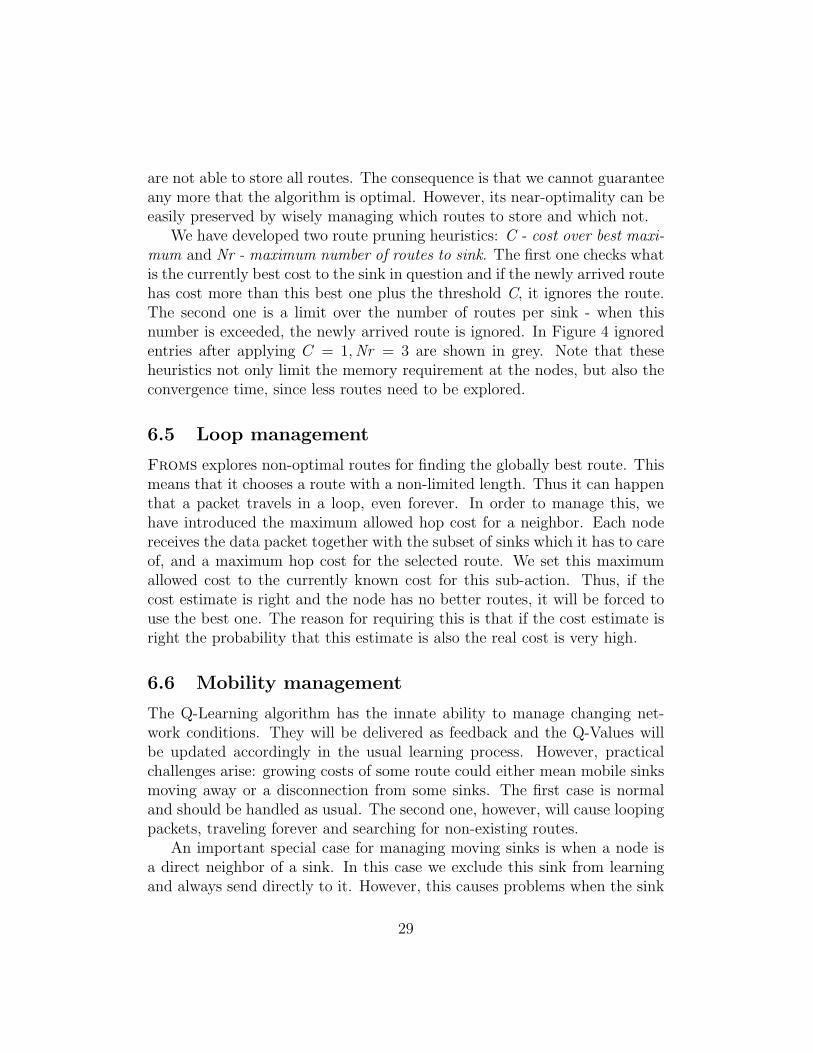
The Q-Learning algorithm has the innate ability to manage changing net-work conditions. They will be delivered as feedback and the Q-Values willbe updated accordingly in the usual learning process. However, practicalchallenges arise: growing costs of some route could either mean mobile sinksmoving away or a disconnection from some sinks. The first case is normaland should be handled as usual. The second one, however, will cause loopingpackets, traveling forever and searching for non-existing routes.

An important special case for managing moving sinks is when a node isa direct neighbor of a sink. In this case we exclude this sink from learningand always send directly to it. However, this causes problems when the sink

29

sink

SinkControl : node 7

last timestamp

direct neighbor

sink 2 -14 sec falsesink 1 -2 sec true

direct timestamp

--2 sec

Figure 5: SinkControl for node E (direct neighbor of sink P from Figures 1and 4).

moves away and the sink needs to be included in normal learning again.Thus, we need a technique to recognize alive sinks moving out of range.

SinkControl is a simple data structure whose goal is to detect moving ordisconnected sinks. It does not affect the Q-Learning algorithm, but managesthe available routes, erasing invalid ones. It stores information about eachknown sink in the network. Figure 5 presents it for the sample topology ofFigure 1. The feedback delivers a last timestamp for each included sink; thisis the last time this neighbor has heard of the sink. If this timestamp is tooold (a threshold parameter), the sink is deleted. This is the case when eitherthe sink itself has failed or disappeared from the network or the network isdisconnected between the sink and the node. In both cases the applicationlayer has to be notified to delete the data delivery task for those sinks androuting to them has to be stopped.

On the other hand, while the sink is “fresh” data delivery can continueeven if the routes’ costs to it are growing. In order to detect sinks in thedirect neighborhood, we also store the last time the node has heard froma sink directly. If the threshold is exceeded, the flag for direct neighbor isdeleted and Froms is notified.

This simple module enables detection of sink mobility and learning of newroutes with minimum communication overhead, the additional last times-tamp feedback. Despite using timestamps, Froms does not require a timesynchronization protocol or any other means of global time. It is enough touse timestamps like in Figure 5: (now − n · sec). The goal is to detect sinks,which are not responsive for a long time.

Obviously, this sink mobility detection can be implemented for any rout-ing protocol. However, it is not sufficient to handle sink mobility: it onlychecks whether a route can exist or not. Finding the optimal route is stillperformed by Froms and its learning and feedback mechanism. Most im-

30

portantly, delivery of data to the sinks continues while recovering the routesand learning the new costs.

6.7 Node failures

Node failures are managed the same way as sink mobility. Each node storesthe last time it heard from any 1-hop neighbor. Additionally, it stores thelast time it routed something to that neighbor. In case the difference betweenboth timestamps exceeds some threshold, the neighbor is deleted. Note thatif this happens by mistake, the next time the node hears again from thisneighbor, the route will be recovered.

Note that unlike many link management protocols, Froms does not useany beacons or periodic full-network broadcasts. Only overhearing of datapackets is used to check the status of neighbors.

6.8 Cost metrics

Here we present Froms innate ability to incorporate different cost functionsto reach different optimization goals. The cost function is used to calculatethe initial Q-Values in Froms. A simple hop-based metric was presentedalready in Section 4 with Equations 1 and 2. Its optimization goal is tofind the shortest shared path for multiple sinks in terms of hops. The hop-based cost function can be easily exchanged with any other cost-per-linkmetric, like energy needed to reach the farthest neighbor, geographic distanceor geographic progress to the sinks, etc. Various cost metrics and theirproperties are summarized in Table 2.

Another example for a cost-per-link function is a latency-based cost met-ric. Here we need to gather latency information during sink announcementto the sensor nodes. The latency needs to represent the radio propagationlatency (where the differences will be negligible for usual sensor networks)and the latency caused by the packet queues on the nodes. However, notethat such a cost metric is what we call here a dynamic cost metric: it isexpected to change during network lifetime and to change fast. For Fromsthis means that it will never globally converge, nor stay in a converged state.However, we show in the next paragraphs other dynamic cost functions andhow to handle their behavior. In fact, we make use of this non-convergingbehavior and turn it into an advantage.

31

Cost met-ric

Calculation ofinitial values

Optimizationgoal

Conver-gence

Dyna-mic

BestQ-Values

simple metrics

Hops∑

hops shortest shared path(Steiner tree)

guaran-teed

no lowest

Latency∑

latency least latency path no yes lowest

Transmissionenergy

∑energies least energy path guaran-

teedno lowest

Geographicdistance

∑dist shortest shared path guaran-

teedno lowest

Aggr. rate∑

rates maximum aggr.path

slow no highest

combined metrics

Hops & rem.battery ofnodes

∑hops ·

hcm(bathops)shortest shared paththrough nodes withhigh battery

no yes lowest

Table 2: Different possible cost metrics for Froms and their main properties.

Here we concentrate on one combined cost metric to demonstrate howto use such complex cost metrics with Froms. We use a combination ofremaining battery on the nodes and minimum hops. In this case we calculatethe Q-Values as a combination of two metrics as follows:

Qcomb(route) = f(Ehops , Ebattery) (10)

where Ehops is the estimated hop cost of the route exactly as we calculateit in equations 1 and 2, and Ebattery is the estimated battery cost of this route,which we define as the minimum remaining battery of all nodes along it:

Ebattery(route) = minni∈route

battery (11)

The function f that combines the two estimates into a single Q-Value isbased on a simple and widely used function:

f(Ehops , Ebattery) = hcm(Ebattery) · Ehops (12)

32

100 90 80 70 60 50 40 30 20 10 0

1

2

3

4

5

battery level [%]

hop

coun

t mul

tiplie

r (hc

m)

hop basedsteep linearlinearexponential

Figure 6: Hop count multiplier (hcm) functions for different optimizationgoals.

hcm is the hop-count-multiplier, a function that weights the hop countestimate based on the remaining battery. For simplicity we drop the “esti-mation” and denote the Q-Value components as hops and battery .

Figure 6 shows four different hcm functions. If the battery level is com-pletely irrelevant, then hcm(battery) is a constant and f(hops , battery) isreduced to a hop-based function only. Instead, if the desired behavior is tolinearly increase f as the battery levels decrease, a linear hcm function shouldbe considered. Figure 6 shows two linear functions. The first (labeled linear),has minimal effect on the routing behavior. For example, a greedy protocolwhich always uses the best (lowest) Q-Values available, when faced with tworoutes with f(1, 10%) = 1.9 and f(2, 100%) = 2, will select the shorter routeeven though the battery is nearly exhausted. Even when faced with longerroutes of length 2 and 3 respectively, it will use the shorter route until itsbattery drops to 40%. Only when their values become f(2, 40%) = 3.2 andf(3, 100%) = 3, the protocol will switch to the longer route. Thus, this trade-off of weighing the hop count of routes (their length) versus the remainingbatteries must be taken into account when defining hcm.

The main drawback of linear hcm functions is that they do not differenti-ate between battery levels in the low and high power domain. For example,a difference of 10% battery looks the same for 20 − 30% and for 80 − 90%.Thus, to meet our goal of spreading the energy expenditure among the nodes,we require an exponential function that starts by slowly increasing the value

33

of hcm with decreasing battery, initially giving preference to shorter routes.However, as batteries start to deplete, it should more quickly increase hcmin order to use other available routes, even if they are much longer, thusmaximizing the lifetime of individual nodes. Of course, such a function givespreference to longer energy-rich routes, and will increase the per packet costsin the network.

The presented battery and hop based function is a dynamic function,which means that it is expected to change during the network lifetime. Ob-viously, the remaining batteries of the nodes will change and thus the Q-Values as well. The major consequence of this is that Froms does not sta-bilize, because the Q-Values never stabilize. However, this is not necessarilya disadvantage: Froms will just continue exploring routes throughout thenetwork lifetime. Combining a dynamic cost function with a mostly greedyexploration strategy will ensure that Froms is not spending too much en-ergy on exploration of routes and is mostly using the best available routes.On the other side, we need to ensure that Froms is still able to find thebest routes. For this, we use the advantage of a dynamic cost function. TheQ-Values change because of the dynamic nature of the cost metric and forceFroms to use different routes (because it mostly selects the best ones): thus,it implicitly forces Froms to explore new routes.

This property of dynamic cost functions we call the dynamic cost advan-tage of implicit exploration, which is a very important property of Froms.It allows Froms to use a very simple greedy or ε-greedy exploration strategywith very low probability for exploration (see next section) and still ensuresthat the optimal routes are found. This simplifies significantly the imple-mentation of Froms both in terms of processing and memory requirementsand make Froms much more intuitive.

Similarly, one can easily design and implement other cost metrics, bothsimple and combined. The used cost function depends on the applicationscenario and needs to be revisited for each deployment. However, the powerof Froms is its innate ability to accommodate nearly any cost function. Thechanges to the protocol are marginal and do not affect its basic functionality.

6.9 Exploration strategies

The exploration strategy controls how Froms chooses between the availableroutes. It also controls the exploration/exploitation ratio, which is respon-sible for both finding the optimal route and minimizing routing costs. In

34

10 20 30 40 50 600

5

10

15FROMS uniform stochastic

[secs]

[epsilo

n | tem

p | E

TX

]

FROMS uniform stochastic

!" #" $" %" &" '""

&

!"

!&()*+,-./01234!56..78-91:;-:.</.6=:>6.

?0.@0A

?./01234-B-:.</-B-CDEA

-

-

FROMS epsilon greedy with temperature

temperature taken routes

best available routes

exploration

best available routes

taken routes

!" #" $" %" &" '""

&

!"

!&()*+,-./01/23456-/734895!61//.:

;3/03<

;/734895-=->/?7-=-@AB<

-

-

/C78912>4950D11/5>-19D>/-093>3E/3>-2F2482E8/-093>3

10 20 30 40 50 600

5

10

15FROMS epsilon greedy 0.3

[secs]

[ep

silo

n | te

mp |E

TX

]

FROMS epsilon greedy

exploration rate

taken routes

best available routes

FROMS decreasing epsilon greedy

exploration rate

taken routes

best available routes

Figure 7: The route selection behavior at the source with different explorationstrategies in a sample 50 node topology with 3 sinks and 1 source.

our preliminary studies [12], we have applied two different techniques forexploration: greedy and probabilistic. The greedy strategy simply ignoresexploration and always chooses between the best available routes. Stochasticexploration strategies on the other hand assign a probability to each of theroutes, depending or not on their current or initial Q-Values, and choose theroutes accordingly. These exploration strategies showed good results, but arevery complicated to implement since they require updating the probabilitiesafter each reward.

Here, we turn to a new set of exploration strategies for two main reasonsfor the main reason of making them more intuitive and simple to implement.The behavior of the considered strategies is depicted in Figure 7.

35

ε - greedy. This strategy is taken directly from the original Q-Learningalgorithm and is very simple to apply and implement: with probability εselect any of the available routes; with probability 1 − ε, select one of thebest routes. Note that when ε = 0 we have the old greedy strategy from [12].

decreasing ε - greedy. This strategy is the same as before, but ad-ditionally decreases ε with time. The reason for this is that usually at thebeginning of the algorithm the Q-Values change a lot, but with time theseupdates become more rare and eventually stop. After convergence it is moreappropriate for Froms to be greedy, since no changes are expected and therouting costs should be as low as possible. ε increases again in case of failuresor mobility.

ε - greedy with temperature. This strategy is again a variation of ε-greedy, but instead of decreasing ε itself, it limits the set of routes presentedto the strategy. At the beginning, with high temperature T , all routes arepresented to the strategy, independent from their current Q-Values. Withdecreasing T , however, only routes with better Q-Values are presented andwith T = 0 only the best routes are presented. ε remains constant and thetemperature is increased in case of failures or mobility.

uniform stochastic with stopping strategy. This strategy is takenfrom our previous work [12] (it performed the best out of all comparedstochastic strategies there) and is used for comparison reasons. It assignsthe same probability to each sub-action and updates it every time a rewardarrives for it, decreasing it with neutral rewards, increasing it with negativerewards, and leaving it the same with positive rewards. It stops explorationcompletely after some number of continuous neutral rewards to the node andstarts it again with negative/positive rewards.

6.10 Summary

In this section we presented all parameters and implementation details ofFroms. The main parameters which need to be specified before deployingFroms are its cost function and exploration strategies. Additionally, nodefailure management is a necessary option in nearly any WSN. However, allother presented modules implement special features, like sink mobility sup-port or route pruning heuristics for extremely memory-resticted hardwaresystems, and need to be deployed only when necessary. In the following sec-

36

tions we present an extensive evaluation of Froms and all of its componentsand features both under simulation and on real hardware.

7 Evaluation methodology and environment

Additionally to the theoretical analysis in Section 5, we use evaluation throughsimulation and on real hardware to show the most of the aspects and prop-erties of Froms. We use a wide range of evaluation metrics across manydifferent network scenarios and parameters. Of course, an exhaustive analy-sis under any possible environmental conditions is not possible for time andspace reasons.

Simulation environment. We use the OMNeT++ network discreteevent simulator, together with its extensions Mobility Framework and prob-abilistic radio propagation models [48]. This is a user friendly environmentwith active development community, easily extendable with our own models.Unfortunately, there are no energy expenditure models, nor realistic MACprotocols for the Mobility Framework. Thus, we needed to implement thefollowing additional simulation models:

• Linear battery model. A linear battery model which accounts fordifferent energy expenditures for radio sleeping, receiving and sending,is sufficient for the evaluation of a routing protocol. We use the energyexpenditure model of Mica2 nodes, see Table 3.

• MAC protocols. We have implemented BMAC [49] and LMAC [50]as representatives of low power listening MAC protocols and TDMAbased protocols. Both have been used for real WSN deployments andare widely accepted by the WSN community. Frame and slot dura-tions were identified experimentally so that all evaluated data trafficmodels are accommodated without MAC buffer overflow. In LMAC wereserved 5 node IDs for mobile nodes to avoid continuous slot changing.

Hardware testbed. We implement and test the developed routing pro-tocol Froms on a real hardware testbed, consisting of 10-15 MSB430 nodesfrom ScatterWeb [51], organized in multi-hop topologies (see Figure 9). Theirmain characteristics are summarized in Figure 8. For implementation we use

37

Layer Protocol/model Parameters

Application regular data reportdata rate: every 10 sec

sink announcement: every100 sec

Routing

Froms

see textunicastDD

multicastDD

MSTEAM

Medium access

LMAC slots: 32

slot length: 60 ms

preamble length: 12 bytes

BMAC slot length: 50 ms

preamble length: 120 bytes

Energy Linear battery SLEEP: 36 mW

expenditure (Mica-2) RX, TX: 117 mW

Radio propagation 1-Nakagami -

Table 3: Summary of simulation environment model for our experiments.

the OS-like ScatterWeb2 library, which provides simple interfaces for send-ing/receiving messages, setting timers, reading sensory data etc. We use theprovided non-persistent idle CSMA MAC protocol without acknowledgments.

Comparative analysis. For conducting a comparative analysis of Froms,we have implemented three well known state-of-the-art routing protocols:

• Msteam [10] is a recent state-of-the-art geographic multicast routingprotocol. The comparison between Msteam and Froms is especiallyinteresting and challenging, as they require different available informa-tion on the nodes to achieve the same goal. Thus, also a general perfor-mance comparison between hop-based and geographic based protocolsis presented. We use the same application layer and sink announce-ment broadcasts for both Froms and Msteam. They have severaladvantages against the typical pre-known set of sink coordinates, usedby many geographic-based protocols. First, it replaces the use of bea-cons for discovering and maintaining neighbors and, second, it enablesrecovery and mobility, which are not covered by the original version

38

MSB430

Provider ScatterWeb, Berlin, GermanyProcessor MSP430Frequency 8MHzMemory 5 KB RAM + 55 KB FlashRadio ChipCon 1020OS ScatterWeb2, TinyOS, Contiki, etc.Other SD-card slot

Figure 8: Characteristics of the MSB430 sensor nodes

of the protocol. Two versions of Msteam are evaluated: the originalMsteam uses cost over progress to sinks metric to evaluate possi-ble next hops, where the cost is a function of the geographic distancebetween the nodes. We also implemented a simplified version, calledMsteam-const, where the cost is always 1 and thus only the progressto the sinks is considered.

We decided to add Msteam to our analysis since it represents a verywell performing class of protocols for multicast applications. Indeed,most of the multicast protocols for WSNs are location-based and wedesire to have a direct comparison with one of them.

• Unicast Directed Diffusion (udd) [11] is a well known, simple,and efficient routing paradigm, where each of the nodes builds gradientstowards the sinks. We label this version of Directed Diffusion ”unicast”(or udd for short), since we consider the original one-phase pull versionof the protocol, as opposed to multicast Directed Diffusion (ormdd), as explained next.

• Multicast Directed Diffusion (mdd) is a multicast-optimizedvariation of udd of our own design [52]. It is searching locally onthe nodes for shared paths for multiple sinks. It can be considered asimplified version of greedy-Froms, which keeps only the best hops toindividual sinks, does not explore, and the cost function is based onhops only. However, it does not incorporate the learning mechanism

39

1

73

4

8 9

5

2

6

10

1

2

3

8

9

7

4

6

5

14

12

15

13

10

11

Figure 9: Topologies 1 (left) and 2 (right) for the real hardware testbed,sinks are shaded, source is node 6.

of Froms, nor it is able to find the globally optimal path unless bychance.

We compare the performance of all here presented routing protocols undersimulation. On the hardware testbed we have implemented only Froms andmdd. We decided against the original Directed Diffusion, because it is aunicast routing protocol and against Msteam, because its implementationis very processing and memory intensive and did not fit on the used hardware.

8 Evaluation of FROMS on the hardware testbed

We compare the performance of Froms with ε-greedy exploration strategyagainst the multicast version of Directed Diffusion of our own design [52].We use two controlled network topologies as given in Figure 9. In theseexperiments, we allowed the nodes to process packets only from some prede-fined set of nodes and to drop immediately all others. We were forced to dothis, because we were unable to create a natural multi-hop topology, whichis essential for the evaluation of the routing protocol [53].

8.1 Memory and processing requirements

Here we present and discuss the memory and processing requirements asobtained from the real hardware testbed. No simulated results are presented,

40

41

42

43

44

45

msec

mDD

2 sinks

mDD

3 sinks

FROMS

2 sinks

FROMS

3 sinks

46

FROMS + ACKs

FROMS

mDD + ACKs

mDD

Scatterweb2

33610

31986

29648

28024

19628

ROM (bytes)

3345

3326

2952

2932

1476

RAM (bytes)

Figure 10: (left) Memory usage at compile time. The Scatterweb libraryalone is given for comparison. (right) Processing time to find a route inmilliseconds for mdd and Froms and max-min intervals.

since they depend strongly on the simulation environment used and are notcomparable to real hardware requirements.

Memory usage. Figure 10 (left) presents the memory footprints atcompile-time for mdd and Froms together with the application layer. Itshows the memory reserved for the flash ROM and the RAM. The footprintof the ScatterWeb2 library alone is given for comparison. The vanilla im-plementation of mdd on top of ScatterWeb2 e.g. consumes roughly 3KB ofRAM at compile time, leaving 2KB for stack allocation and application-levelprotocols. Compared to the standalone implementation of ScatterWeb2, thisis negligible.

Both implementations of Froms and mdd use static data structures,because there is no working dynamic memory management implementationfor the microprocessor of the used hardware platform MSB430. No routestorage heuristics are used for Froms and thus all possible routes are keptat all times. Thus the data structures are already included also in the memoryfootprints in Figure 10. Although Froms’s data structures are more complexand large than the routing table of mdd, its memory requirements are notsignificantly higher. mdd has a very tiny data structure, but despite this, itsimplementation size is not negligible. In fact, the majority of its memory isused for the functionality of the protocol, not for data structures.

Processing time. We measured the time needed to find a route for each

41

82 % 94 %

mDD FROMS

50 %

100 %

deliv

ery

rate

cost

s pe

r pac

ket i

n ET

X

6

3

4

5

7

topo 1, sinks 2mDD FROMStopo 1, sinks 3

mDD FROMStopo 2, sinks 2

mDD FROMStopo 2, sinks 3

71 %87 % 83 % 94 %

64 % 74 %

cost per received packetcost per generated packetoptimal (Steiner tree) cost

9

8

10

mDD FROMStopo 1, sinks 2

mDD FROMStopo 1, sinks 3

mDD FROMStopo 2, sinks 2

mDD FROMStopo 2, sinks 3

Figure 11: Routing costs and delivery rates for Froms and mdd in variousnetwork scenarios.

packet in the network at every node in milliseconds. Basically, we discoveredthat it takes slightly longer to find a route to more sinks but the differencebetween the protocols is very small. The results in Figure 10 (right) aresummarized based on the number of sinks in the network. They are obtainedfrom experiments with topology 2 only. The reason why Froms needs moretime to find a route for a data packet is its routing data structure. We needto search through all of the available routes to find the best available one.Consequently, with 3 sinks the processing time increases further.

These results are an important proof of the applicability of Froms andin general of reinforcement learning based communication protocols on realhardware. They show that Froms is easily implementable and that its mem-ory and processing requirements are negligibly higher than those of a verysimple routing protocol like mdd. The comparative evaluation of both pro-tocols on the real testbed is discussed later in Section 8.2.

42

82 % 88 % 87 %

DD, 2 sinksno 1 ms 100 ms

70 % 78 %

DD, 3 sinksno 100 ms

94 % 94 % 99 %

FROMS, 2 sinksno 1 ms 100 ms

87 % 99 %

FROMS, 3 sinksno 100 ms

50 %

100 %

deliv

ery

rate

cost

s pe

r pac

ket i

n ET

X

0

6

1

2

3

4

5

7cost per received packetcost per generated packetoptimal (Steiner tree) cost

DD, 2 sinks DD, 3 sinks FROMS, 2 sinks FROMS, 3 sinks

Figure 12: In-network performance when applying transmission backoff, re-sults from topology 1.

8.2 Comparative analysis

Next, we compare the performance of Froms and mdd on real hardware interms of delivery rate and routing costs. Figure 11 summarizes the results forseveral network configurations. As expected from our simulation experimentsand theoretical analysis, Froms achieves lower routing costs. This can beattributed to its learning algorithm which actively explores the network foroptimal routes. We also compare the performance against the theoreticallyoptimal cost of the Steiner tree.

In simulation we are unable to measure accurate delivery rates since trans-mission failures cannot be reliably simulated. Here, instead, we confirm ourtheoretical expectation that Froms is able to achieve higher delivery ratein any network scenario. Data is lost in mdd mainly due to the higherin-network communication caused by the periodic sink announcements (seeSection 9) and the longer routes to the sinks. This increases the traffic andcollision probability leading to packet losses. Figure 11 supports these ob-servations, showing that the delivery rate of both protocols clearly drops innetworks with larger numbers of nodes and sinks.

Figure 12 presents the results when using transmission backoff, clearly

43

83 %94 %

DD FROMS

50 %

100 %

deliv

ery

rate

cost

s pe

r pac

ket i

n ET

X

8

4

6

10

no acks, no backoffDD FROMS

acks, no backoffDD FROMS

acks, backoff 1ms

91 % 98 % 94 %100 %

16

12

14cost per received packetcost per generated packetoptimal (Steiner tree) cost

DD FROMSno acks, no backoff

DD FROMSacks, no backoff

DD FROMSacks, backoff 1ms

Figure 13: In-network performance when using acknowledgments, resultsfrom topology 2.

showing that the technique is highly effective at improving delivery rates.We implemented a simple algorithm in which a parameter (in our case 0,1 or 100 ms) is multiplied with the node’s ID and this delay is applied be-fore forwarding any packet. This backoff reduces packet collisions and thusincreases successful delivery.

Another common mechanism to increase the delivery rate is to forcepacket acknowledgments. We use overhearing of DATA packets as implicit ac-knowledgments, avoiding additional costs. Figure 13 shows how routing costsskyrocket, while the delivery rate also increase. The incurred overhead stemsfrom re-sending unacknowledged packets. Communication failures cause notonly data loss, but also loss of acknowledgments. This results in resendingpackets which were actually received, but not acknowledged. Consequently,the communication traffic explodes, leading to even higher loss rates.

44

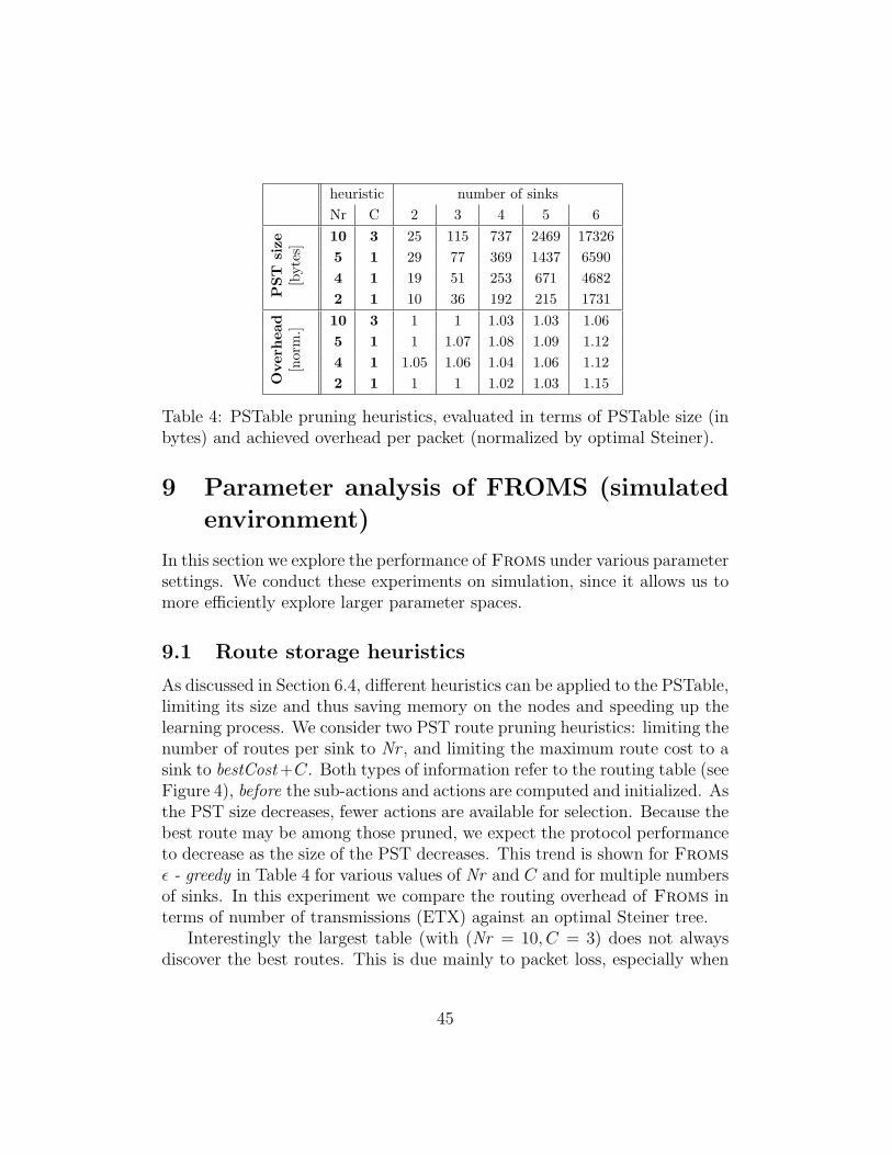
heuristic number of sinksNr C 2 3 4 5 6

PST

size

[byt

es] 10 3 25 115 737 2469 17326

5 1 29 77 369 1437 65904 1 19 51 253 671 46822 1 10 36 192 215 1731

Ove

rhea

d[n

orm

.]

10 3 1 1 1.03 1.03 1.065 1 1 1.07 1.08 1.09 1.124 1 1.05 1.06 1.04 1.06 1.122 1 1 1 1.02 1.03 1.15

Table 4: PSTable pruning heuristics, evaluated in terms of PSTable size (inbytes) and achieved overhead per packet (normalized by optimal Steiner).

9 Parameter analysis of FROMS (simulated

environment)

In this section we explore the performance of Froms under various parametersettings. We conduct these experiments on simulation, since it allows us tomore efficiently explore larger parameter spaces.

9.1 Route storage heuristics

As discussed in Section 6.4, different heuristics can be applied to the PSTable,limiting its size and thus saving memory on the nodes and speeding up thelearning process. We consider two PST route pruning heuristics: limiting thenumber of routes per sink to Nr , and limiting the maximum route cost to asink to bestCost +C. Both types of information refer to the routing table (seeFigure 4), before the sub-actions and actions are computed and initialized. Asthe PST size decreases, fewer actions are available for selection. Because thebest route may be among those pruned, we expect the protocol performanceto decrease as the size of the PST decreases. This trend is shown for Fromsε - greedy in Table 4 for various values of Nr and C and for multiple numbersof sinks. In this experiment we compare the routing overhead of Froms interms of number of transmissions (ETX) against an optimal Steiner tree.

Interestingly the largest table (with (Nr = 10, C = 3) does not alwaysdiscover the best routes. This is due mainly to packet loss, especially when

45

the number of sinks in the network increases. This causes higher data trafficand thus more data loss.

In the remainder of our experiments, however, we do NOT use any routepruning heuristics in order to limit the number of used parameters and sim-plify evaluation and understanding of the results. Furthermore, as we alreadyshowed in the previous Section 8.1, we are able to implement Froms withno route pruning heuristics on real hardware. In case the implementationneeds to be restricted because of a very large number of sinks or very highdensity of the nodes, we suggest using a moderate size for the PSTable with(Nr = 4, C = 1) that yields route costs close enough to optimal.

9.2 Exploration strategies

In the next paragraphs we explore the behavior and performance of Fromswith different exploration strategies. We consider the following four types ofstrategies: ε - greedy, ε - greedy with temperature, decreasing ε - greedy anduniform-stochastic (see also Section 6.9).

The experimental results are shown in Figure 14. In the top graphs wefix the number of nodes to 50, the number of sources to 1 and vary thenumber of sinks from 1 to 5. All exploration strategies are normalized byFroms decreasing ε-greedy. The deviation of the first node death time (leftgraph) is only insignificant and does not exceed 1%. On the other hand,the differences in the routing overhead (number of ETX per delivered packetin the network) reaches 10%. This deviation is a result of the MAC layer.BMAC uses only broadcast transmissions. This diminishes small differencesin the number of sent packets (ETX) from the routing layer, and shows howimportant the MAC layer is for minimizing the energy spent and maximizingnetwork lifetime. On the other hand, less traffic is always an advantage sinceit increases the delivery rate and thus the overall efficiency of the network.

The rest of the graphs in Figure 14 present experiments with varyingnumber of sources and nodes respectively. They support the above madeobservations. Given the results obtained in this step, we will consider twoexploration strategies in our comparative analysis experiments: decreasingε-greedy with ε = 0.5 and ε-greedy with ε = 0.1.

46

0 1 2 3 4 5 6

1.002

1.

0.998

0.996

0.994

0.992

0.99number of sinks

time

(nor

mal

ized)

First node death comparison, BMAC

FROMS decr 05FROMS greedy 01FROMS greedy 03FROMS tempFROMS uniform

0 1 2 3 4 5 6

1

1.02

1.04

1.06

1.08

1.1

number of sinks

ET

X (

no

rma

lize

d)

Routing overhead after 2000 secs, BMAC

FROMS decr 05

FROMS greedy 01

FROMS greedy 03

FROMS temp

FROMS uniform

over

head

(nor

mal

ized

)

0 1 2 3 4 5 60.96

0.965

0.97

0.975

0.98

0.985

0.99

0.995

1

1.005

1.01

number of sources

time

(nor

mal

ized)

First node death comparison, BMAC

FROMS decr 05FROMS greedy 01FROMS greedy 03FROMS tempFROMS uniform

0 1 2 3 4 5 60.95

1

1.05

1.1

1.15

1.2

1.25

number of sources

ET

X (

no

rma

lize

d)

Routing overhead for 2000 secs, BMAC

FROMS decr 05

FROMS greedy 01

FROMS greedy 03

FROMS temp

FROMS uniform

over

head

(nor

mal

ized

)

50 75 100 125 150 175

0.988

0.99

0.992

0.994

0.996

0.998

1

1.002

number of nodes

time

(nor

mal

ized)

First node death comparison, BMAC

FROMS decr 05FROMS greedy 01FROMS greedy 03FROMS tempFROMS uniform

50 75 100 125 150 175 2000.99

1

1.01

1.02

1.03

1.04

1.05

number of nodes

ET

X p

er

de

live

red

pa

cke

t

Routing overhead for 2000 secs, BMAC

FROMS decr 05

FROMS greedy 01

FROMS greedy 03

FROMS temp

FROMS uniform

over

head

(nor

mal

ized

)

Figure 14: Evaluation of exploration strategies, mean over 50 different topolo-gies, 5 runs each; the network consists of (top) 50 nodes, 1 source and 1-5sinks; (middle) 50 nodes, 1-5 sources and 3 sinks; (bottom) 50-200 nodes, 1source and 2 sinks. All experiments performed with BMAC.

47

9.3 Cost functions

As we already showed in Section 6.8, Froms can work with nearly any costfunction: hops, location information, remaining energy on the nodes, delay,etc. An important property of the used cost function is its localized nature, asFroms allows direct exchange of information only among one-hop neighbors.The cost function in Froms is used in three places - initialization of routecosts, computation of costs to reach some neighbor and comparison betweenroutes. All these functions are independent from the rest of Froms and canbe easily exchanged.

In this section we concentrate on two main cost functions: a hop-basedone and a combined hop and remaining energy based one, as already intro-duced in Section 6.8. Recall that the goal of the first one, hop function, isto select globally shortest routes to reach all sinks. Instead, the second one,hop-battery function, favors shorter routes with higher remaining batteriesof the involved nodes, thus spreading the energy expenditure throughout allnodes of the network. Everything else in the Froms implementation remainsthe same: data structures, exploration strategies, feedback, etc.

Figure 15 presents different metrics for two exploration strategies of Fromswith both cost functions. The hop-battery cost functions slightly extends thenetwork lifetime: however, only by at most 1% (top left graph). This is dueto the nature of the cost function: on one side, it uses nodes more uniformlyand this can be observed in the standard deviations of remaining energiesat the nodes from the top right graph. In fact, the hop-battery cost func-tions decreases the standard deviation of the remaining energies by 10-15%.However, at the same time Froms is forced to use longer routes and therouting overhead increases (bottom left graph). These two effects combineinto a slightly increased lifetime and slightly decreased spent energy, but thedifference to the hop-based cost metric is only insignificant.

Our previous study in a less realistic simulation environment (MATLAB)in [13] showed different results. In that study we achieved a significantlylonger network lifetime (by nearly 80%) because the nodes in the networkwere used more uniformly for routing. However, in a more realistic wirelesssimulation with a real implementation of a MAC protocol, overhearing ofpackets among neighbors cannot be avoided and spends a lot of energy. Evenwhen switching to alternative routes with higher batteries, the hop-batterycost function selects routes near to the last used ones, thus further drainingthe batteries of the nodes. An extreme example are the direct neighbors

48

0 1 2 3 4 5 60.995

1

1.005

1.01

1.015

number of sinks

time

(nor

mal

ized)

First node death comparison, LMAC

FROMS decr 0.5FROMS decr 0.5 batteryFROMS greedy 0.1FROMS greedy 0.1 battery

0 1 2 3 4 5 60.8

0.85

0.9

0.95

1

1.05

1.1

1.15

1.2

1.25

1.3

number of sinks

perc

ent (

norm

alize

d)

Standard deviation of the mean energy at first node death, LMAC

FROMS decr 0.5FROMS decr 0.5 batteryFROMS greedy 0.1FROMS greedy 0.1 battery

0 1 2 3 4 5 60.99

1

1.01

1.02

1.03

1.04

1.05

1.06

1.07

1.08

number of sinks

ET

X p

er

de

live

red

pa

cke

t [n

orm

aliz

ed

]

Routing communication overhead, LMAC

FROMS decr 0.5

FROMS decr 0.5 battery

FROMS greedy 0.1

FROMS greedy 0.1 battery

over

head

per

del

iver

ed p

acke

t (no

rmal

ized

)

0 1 2 3 4 5 60.995

0.996

0.997

0.998

0.999

1

1.001

number of sinks

mA

(n

orm

aliz

ed

)

Total energy spent [mA] after 2000 secs, LMAC

FROMS decr 0.5

FROMS decr 0.5 battery

FROMS greedy 0.1

FROMS greedy 0.1 battery

spen

t ene

rgy

(nor

mal

ized

)

Total energy spent for 2000 secs, LMAC

Figure 15: Comparison for two different exploration strategies of Fromswith hop-based cost and hop-battery based cost. All experiments performedwith LMAC.

of the source: whatever route is taken to the sinks, the neighbors of thesource always overhear the packets and drain their batteries. In fact, wediscovered that usually either the source itself, neighbors of the source, ordirect neighbors of the sinks are the first to die.

However, battery-hop cost functions are a good solution when the datadelivery task to the sinks is short. In such cases, the cost function is ableto spread the usage of the nodes more uniformly, thus avoiding buildinglow-battery bottlenecks in the network.

49

10 Comparative evaluation of FROMS in sim-

ulation

We compare the performance of Froms against three other state-of-the-art routing protocols: multicast Directed Diffusion (mdd), unicast DirectedDiffusion (udd) and Msteam. We explore all of the routing protocols interms of their routing overhead, network lifetime, standard deviation of theremaining energy on the nodes, and total spent energy in various networkscenarios, including mobile sinks and node failures. We use the simulationenvironment as described in Section 7.

10.1 Multi-source multi-sink routing

In this section we make an extensive scalability analysis and comparisonbetween Froms, Msteam, mdd and udd, as outlined in Section 7. Similarto the stand-alone evaluation of Froms in the previous Section 9 we fix allnetwork parameters except for one and give mean results over 50 differentrandom connected topologies with 5 random runs each. Figure 16 presentsthe obtained results for different number of sinks (top), number of sources(middle) and number of nodes (bottom) while using BMAC as MAC layerprotocol. The achieved results with LMAC were very similar and graphsare omitted. The first point of Froms (e.g. one sink, one source or 50nodes) is used as the point of normalization. Unlike the experiments for thestand-alone evaluation of Froms in Section 9, here we are interested in thescalability analysis and comparison of all routing protocols. Thus, we needto use only a single point for normalizing the results and not a full line.

Coming back to Figure 16, with increasing number of sinks, all protocolsspend more energy. However, Froms achieves the least energy expenditurecompared to the other protocols. This is due to two reasons: its ability tofind optimal multicast routes and the limited use of broadcast sink announce-ments. The lower energy expenditure of Froms compared to mdd are alsodue to these reasons. However, it is interesting to note that Msteam (bothvariations) reaches energy spendings well over mdd and Froms. In fact,Msteam-const (where the cost of sending a packet between two nodes isconsidered to be constant) performs much better than the original Msteamprotocol. This is due to the fixed transmission power of the simulated nodes(which is often also the case in real hardware). The original Msteam proto-

50

0 1 2 3 4 5 61

1.05

1.1

1.15

1.2

1.25

number of sinks

mA

(n

orm

aliz

ed

)

Total energy spent [mA] after 2000 secs, BMAC

FROMS decr 05

mDD

MSTEAM

MSTEAM const

uDD

spen

t ene

rgy

(nor

mal

ized

)

Total energy spent for 2000 secs, BMAC

0 1 2 3 4 5 60.5

1

1.5

2

2.5

3

3.5

4

4.5

5

number of sinks

pe

rce

nt

(no

rma

lize

d)

Standard deviation of the mean energy after 2000 secs, BMAC

FROMS decr 05

mDD

MSTEAM

MSTEAM const

uDD

stan

dard

dev

iatio

n (n

orm

aliz

ed)

0 1 2 3 4 5 61

1.05

1.1

1.15

1.2

1.25

1.3

number of sources

mA

(n

orm

aliz

ed

)

Total energy spent [mA] after 2000 secs, BMAC

FROMS decr 05

mDD

MSTEAM

MSTEAM const

uDD

spen

t ene

rgy

(nor

mal

ized

)

Total energy spent for 2000 secs, BMAC

0 1 2 3 4 5 61

1.5

2

2.5

3

3.5

4

4.5

number of sources

pe

rce

nt

(no

rma

lize

d)

Standard deviation of the mean energy after 2000 secs, BMAC

FROMS decr 05

mDD

MSTEAM

MSTEAM const

uDD

stan

dard

dev

iatio

n (n

orm

aliz

ed)

50 75 100 125 150 175 2000.96

0.98

1

1.02

1.04

1.06

1.08

1.1

1.12

1.14

1.16

number of nodes

mA

(n

orm

aliz

ed

)

Total energy spent [mA] after 2000 secs per node, BMAC

FROMS decr 05

mDD

MSTEAM

MSTEAM const

uDD

spen

t ene

rgy

(nor

mal

ized

)

Total energy spent for 2000 secs, BMAC

50 75 100 125 150 175 2000.5

1

1.5

2

2.5

3

number of nodes

pe

rce

nt

(no

rma

lize

d)

Standard deviation of the mean energy after 2000 secs, BMAC

FROMS decr 05

mDD

MSTEAM

MSTEAM const

uDD

stan

dard

dev

iatio

n (n

orm

aliz

ed)

Figure 16: Evaluation of routing protocols in terms of total spent energyand standard deviation of remaining energy after the first 2000 seconds, 50different topologies, 5 runs each; the network consists of (top) 50 nodes, 1source and 1-5 sinks; (middle) 50 nodes, 1-5 sources and 3 sinks and (bottom)50-200 nodes, 1 source and 3 sinks. All experiments performed with BMAC.

51

col uses a special cost function, which increases the cost of sending a packetwith increasing distance between the nodes. This cost function is based ongeographic distance rather than taken from real experimental data and thusforces the protocol to take more, shorter hops instead of less long hops.

Froms clearly outperforms any of the protocols in this comparative anal-ysis in terms of energy expenditure, but especially the geographic-based pro-tocol Msteam. The reason for this is the so-called face routing in geo-graphic protocols, which handles void areas (nodes with no progress againstthe sinks). In these cases, the packet is sent back and follows a predefinedroute over a ”face” until reaching again a node with some positive progresstowards the sinks. However, this face route is possibly very long. Second,and more importantly, the exact same route will be taken for each packet,including the sending back of the packet. This incurs excessive and unneededrouting overhead, where reinforcement learning will avoid the repetitive send-ing to void nodes and back.

The same observations can also be made for varying number of sourcesin Figure 16 (middle). In contrast, Figure 16 (bottom) shows the goodscalability of all protocols when varying the number of nodes (the density ofthe network is constant). This is due to the localized nature of all protocols,which are independent of the size of the network. The comparative analysis,therefore, shows exactly the same trend as before. We have observed thesame order of the protocols’ performance also in terms of first node deathand routing overhead per packet (graphs omitted for space considerations).

In summary, Froms achieves between 10 and 22% longer network life-times in terms of first node death, around 2 times less routing overhead,between 5 and 15 % less spent energy and 2 to 3 times lower standard devia-tion of the remaining energies against the other compared routing protocols.The second best protocol in terms of these metrics is mdd. Next comes theconstant-cost variation Msteam-const, then udd and then the originalMsteam protocol.

Last, we present a comparison of all routing protocols over BMAC andLMAC, see Figure 17. This comparison is not intended as an evaluation ofthe MAC protocols in use. Its goal is rather to show the importance of cross-layer design between routing and MAC protocols. In fact, LMAC achieveslonger network lifetime (by 20-25%) and lower energy expenditure (by 20-25%) against BMAC in the network scenarios which we explored. Thus,in our scenarios LMAC is the better choice. However, this evaluation willprobably change with different data rates in the network and another choice

52

0 1 2 3 4 5 60.3

0.4

0.5

0.6

0.7

0.8

0.9

1

number of sinks

time

(nor

mal

ized)

First node death comparison

FROMS decr 0.5 LMACFROMS decr 0.5 BMACmDD LMACmDD BMACMSTEAM LMACMSTEAM BMACuDD LMACuDD BMAC

0 1 2 3 4 5 6

1

1.05

1.1

1.15

1.2

1.25

1.3

1.35

1.4

1.45

number of sinks

mA

(n

orm

aliz

ed

)

Total energy spent [mA] after 2000 secs

spen

t ene

rgy

(nor

mal

ized

)

Total energy spent for 2000 secs, BMAC

Figure 17: Joint comparison of routing protocols with LMAC and BMAC.

2 3 5 7 100.8

0.9

1

1.1

1.2

1.3

1.4

1.5

1.6

1.7

number of failed nodes

mA

(n

orm

aliz

ed

)

Total energy spent [mA] for 2000 secs, BMAC

FROMS decr 05

FROMS greedy 01

mDD

MSTEAM const

uDD

spen

t ene

rgy

(nor

mal

ized

)

Total energy spent for 2000 secs, BMAC Total energy spent for 2000 secs, BMAC

2 3 5 7 100.75

0.8

0.85

0.9

0.95

1

number of failed nodes

pe

rce

nt

(no

rma

lize

d)

Delivery rate for 2000 secs, BMAC

FROMS decr 05

FROMS greedy 01

mDD

MSTEAM const

uDD

deliv

ery

rate

(nor

mal

ized

)

Figure 18: Comparison of delivery rate and spent energy for different routingprotocols with varying number of failed nodes in the network.

of a MAC protocol might be necessary.

10.2 Recovery after failure

An important feature of Froms is its ability to recover quickly after nodefailures. The protocol keeps track of which neighbors are responding andwhich are not, as explained in Section 10. In case some neighbor is notreachable any more, Froms switches directly to the next best route. Thenew costs are propagated as feedback through the network and learned atall affected nodes. In this section we compare the performance of the fourrouting protocols in various node failure scenarios.

We have designed a failure experiment where all but a small set of nodes

53

are given full battery levels. The small set of nodes is given only one thirdof the usual battery level and are thus expected to die quickly one afteranother. We consider this scenario more realistic compared to a controlledkilling of nodes at some predefined time, since in real deployments nodes donot die simultaneously. The results of the experiment in terms of deliveryrate achieved and total spent energy are given in Figure 18 for a set sizeof failed nodes between 2 and 10 (approximately 4 − 20% of all nodes).Each point represents a mean over 50 different topologies, with 30 differentrandom sets of failed nodes. Note that results are gathered only for connectedtopologies. In case failing of nodes actually disconnected the topology, thescenario was ignored. The achieved standard deviation of the experiments isaround 2.3− 3%.

Froms achieves the highest delivery rate and the least energy spent.This is mainly due to the availability of alternative routes at each nodeand the feedback, which quickly propagates through the network, not onlyrecovering routes but recovering the best ones. Similarly, mdd also monitorsthe neighborhood through the Froms node failure detection module, andhas alternative routes at the nodes. Its achieved delivery rate is 2-5% lessthan the one for Froms, due to the learning behavior of Froms. On theother side, Msteam (we tested here only the better performing constant costvariation of Msteam) uses much longer routes (see again Section 10), whichincur more packet loss. Additionally, the neighborhood failure detection doesnot work as efficiently as for Froms and mdd because Msteam uses exactlythe same route over and over again. Thus, in the case of failures of somenodes on a route, it will still be used until the failure detection module deletesthe neighbor. Only then will an alternative be used, which might again havefailed. In contrast, mdd and Froms use same-cost alternative routes in around-robin manner and thus spread the risk of taking a failed route. Forudd the scenario becomes even worse, since it relies on a single route whichneeds to be updated by sink announcements.

In terms of energy expenditure, Froms ε-greedy performs the best, be-cause of its continuous exploration. Instead of exploring only on demand,ε-greedy keeps track of all possible routes and updates their costs proactively.Thus, when a failure is detected, not only an alternative route is available,but its quality is up-to-date and the best possible route can be taken. Addi-tional exploration and taking of non-optimal routes is avoided, delivery rateis increased because of shorter routes (Figure 18 right), and spent energy isminimized (Figure 18 left).

54

1 2 30.9

1

1.1

1.2

1.3

1.4

1.5

1.6

1.7

1.8

1.9

number of mobile sinks

mA

(n

orm

aliz

ed

)Total energy spent [mA] for 2000 secs, 3 sinks in the network

Total energy spent for 2000 secs, 3 sinks, BMACsp

ent e

nerg

y (n

orm

aliz

ed)

Total energy spent for 2000 secs, 3 sinks, BMAC

1 2 30

0.1

0.2

0.3

0.4

0.5

0.6

0.7

0.8

0.9

1

number of mobile sinks

pe

rce

nt

(no

rma

lize

d)

Delivery rate for 2000 secs, 3 sinks in the network

uDD, 100

uDD, 50

FROMS decr 0.5, 100

FROMS greedy 0.1, 100

mDD, 50

mDD, 100

MSTEAM const, 100

MSTEAM const, 50

deliv

ery

rate

(nor

mal

ized

)

Figure 19: Evaluation of all routing protocols with various number of mobilesinks in the network.

In summary, keeping alternative routes, using shortest possible routes,and keeping track of the real length of all available routes (not only of theshortest ones), is a good strategy to be able to recover quickly after failures.

10.3 Sinks mobility

For testing the performance of the routing protocols under scenarios with sinkmobility, we designed two different experiments: one with different numbersof mobile sinks, and a second with different velocities of the mobile sinks.The experiments for both of them were conducted over 50 random topologies,with 10 random runs on each. We achieved a standard deviation of the resultsof 1.6− 1.9%.

The results from the first experiment are presented in Figure 19. Here,we used a network size of 50 nodes, with 3 sinks and 1 source. We variedthe number of mobile sinks from 1 to 3, leaving the rest of them static. Thevelocity of the mobile sinks is constant and is set to 1m/s. We varied the sinkannouncement periods for mdd, udd, and Msteam-const. The assumptionis that refreshing the routes on the nodes more often would lead to betterdelivery rate and shorter routes in case of mobile sinks. This can be seenfor all protocols in Figure 19 (right). In fact, the delivery rate compared tolonger sink announcement periods increases slightly. However, this happensonly at the cost of increasing data traffic and thus higher energy expenditure.Figure 19 (left) shows that energy expenditure increases non-proportionallyto the achieved gain in delivery rate, and is thus not worth it.

55

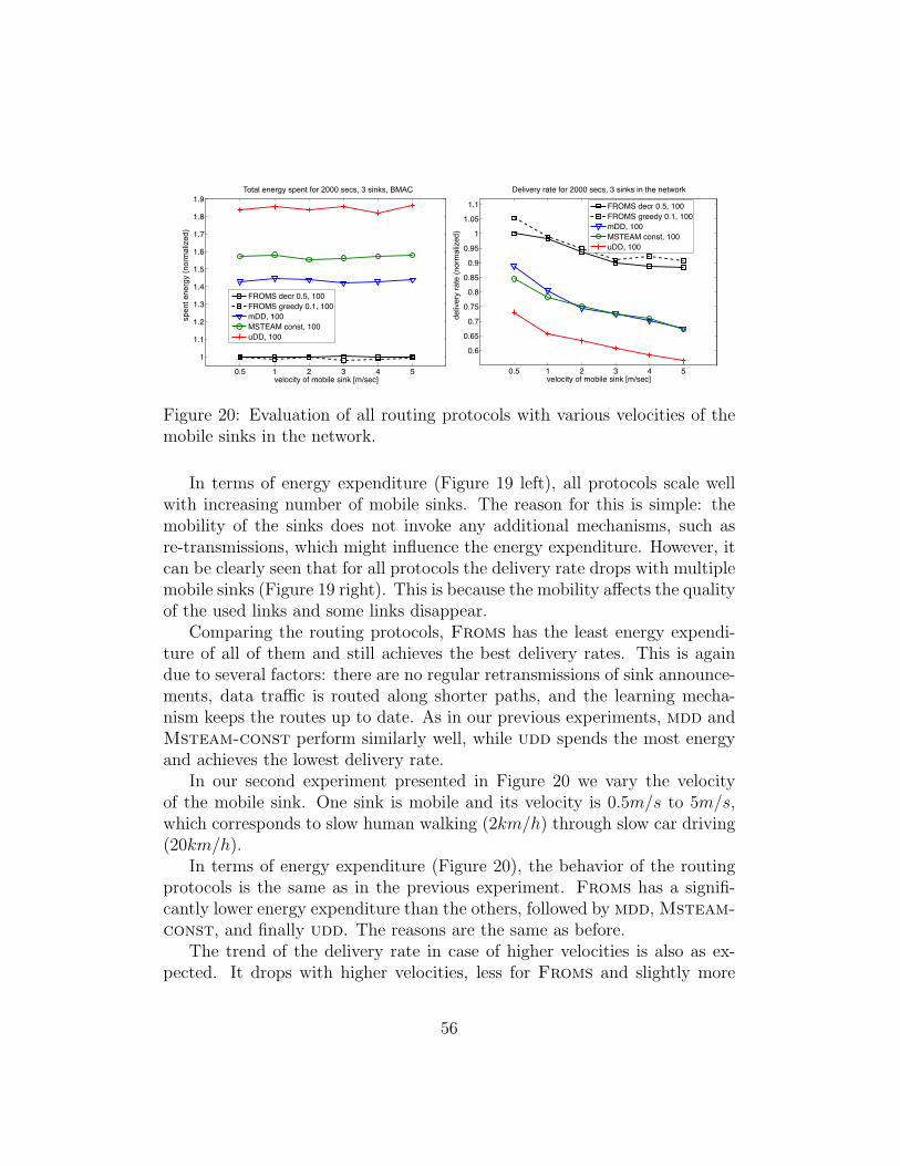
0.5 1 2 3 4 5

1

1.1

1.2

1.3

1.4

1.5

1.6

1.7

1.8

1.9

velocity of mobile sink [m/sec]

mA

(n

orm

aliz

ed

)Total energy spent [mA] for 2000 secs, 3 sinks in the network

FROMS decr 0.5, 100

FROMS greedy 0.1, 100

mDD, 100

MSTEAM const, 100

uDD, 100

Total energy spent for 2000 secs, 3 sinks, BMACsp

ent e

nerg

y (n

orm

aliz

ed)

Total energy spent for 2000 secs, 3 sinks, BMAC

0.5 1 2 3 4 5

0.6

0.65

0.7

0.75

0.8

0.85

0.9

0.95

1

1.05

1.1

velocity of mobile sink [m/sec]

pe

rce

nt

(no

rma

lize

d)

Delivery rate for 2000 secs, 3 sinks in the network

FROMS decr 0.5, 100

FROMS greedy 0.1, 100

mDD, 100

MSTEAM const, 100

uDD, 100

deliv

ery

rate

(nor

mal

ized

)

Figure 20: Evaluation of all routing protocols with various velocities of themobile sinks in the network.

In terms of energy expenditure (Figure 19 left), all protocols scale wellwith increasing number of mobile sinks. The reason for this is simple: themobility of the sinks does not invoke any additional mechanisms, such asre-transmissions, which might influence the energy expenditure. However, itcan be clearly seen that for all protocols the delivery rate drops with multiplemobile sinks (Figure 19 right). This is because the mobility affects the qualityof the used links and some links disappear.

Comparing the routing protocols, Froms has the least energy expendi-ture of all of them and still achieves the best delivery rates. This is againdue to several factors: there are no regular retransmissions of sink announce-ments, data traffic is routed along shorter paths, and the learning mecha-nism keeps the routes up to date. As in our previous experiments, mdd andMsteam-const perform similarly well, while udd spends the most energyand achieves the lowest delivery rate.

In our second experiment presented in Figure 20 we vary the velocityof the mobile sink. One sink is mobile and its velocity is 0.5m/s to 5m/s,which corresponds to slow human walking (2km/h) through slow car driving(20km/h).

In terms of energy expenditure (Figure 20), the behavior of the routingprotocols is the same as in the previous experiment. Froms has a signifi-cantly lower energy expenditure than the others, followed by mdd, Msteam-const, and finally udd. The reasons are the same as before.

The trend of the delivery rate in case of higher velocities is also as ex-pected. It drops with higher velocities, less for Froms and slightly more

56

for the other protocols. The difference comes from the learning mechanismof Froms, which not only substitutes the sink announcement re-broadcasts,but enables faster recovery of routes.

In summary, these experiments show clearly the innate ability of Fromsand its learning algorithm to quickly recover routes in case of mobile sinks,even for a moderate velocity of 20km/h. Compared to all the other routingprotocols, it spends significantly less energy, incurs less data traffic, andachieves considerably higher delivery rates.

11 Future directions and open issues

Current routing protocols, including Froms, consider route characteristicsbased on the properties of the nodes involved in routing, such as the numberof hops, remaining battery levels etc. However, during our work on Froms welearned that the properties of the neighboring nodes are equally important:e.g., a node which is a neighbor of two independent routes drains its batterytwice as quickly as the forwarding nodes because of message overhearing fromboth routes. In the future we plan to incorporate this observation into ourmodel and spread the battery expenditure among all nodes, whether theyare involved in routing or not.

Additionally, we plan to design and implement a multicast MAC protocol,as briefly discussed in Section 6. This will enable us to compare the gainfrom delivering rewards to all overhearing nodes against the saved energyfrom avoiding overhearing.

This paper presented two important contributions. First, it introducedand evaluated Froms, a highly flexible and robust multicast routing proto-col. The results achieved under various environments and network scenariosclearly demonstrate its outstanding performance compared to three otherstate of the art routing protocols. However, even more importantly, this pa-per demonstrated the applicability and the potential of machine learning forsolving hard problems in WSNs. We showed that learning can be efficientlyimplemented on real WSN hardware, that it is fully distributed and that itachieves better results in uncertain and unreliable environments compared toany traditional routing protocols. Encouraged by these results and the ex-perience gathered with Froms, we plan to apply reinforcement learning andother machine learning techniques to other WSN problems. We will exploretheir potential for clustering, neighborhood management, medium access and

57

data modeling.

References

[1] J. M. Kahn, R. H. Katz, K. S. J. Pister, Next century challenges: mo-bile networking for “Smart Dust”, in: Proceedings of the 5th annualACM/IEEE international conference on Mobile computing and network-ing (MobiCom), Seattle, WA, USA, 1999, pp. 271–278.

[2] G. Werner-Allen, K. Lorincz, M. Ruiz, O. Marcillo, J. Johnson, J. Lees,M. Welsh, Deploying a wireless sensor network on an active volcano,IEEE Internet Computing 10 (2) (2006) 18–25.

[3] K. Martinez, P. Padhy, A. Riddoch, R. Ong, J. Hart, Glacial Envi-ronment Monitoring using Sensor Networks, in: Proceedings of the1st Workshop on Real-World Wireless Sensor Networks (REALWSN),Stockholm, Sweden, 2005, p. 5pp.

[4] K. Langendoen, A. Baggio, O. Visser, Murphy loves potatoes: experi-ences from a pilot sensor network deployment in precision agriculture, in:Proceedings of the 20th International Symposium on Parallel and Dis-tributed Processing Symposium (IPDPS), Rhodes Island, Greece, 2006,p. 8pp.

[5] I. F. Akyildiz, W. Su, Y. Sankarasubramaniam, E. Cayirci, Wirelesssensor networks: a survey, Computer Networks 38 (4) (2002) 393–422.

[6] E. Cayirci, T. Coplu, SENDROM: sensor networks for disaster reliefoperations management, Wireless Networks 13 (3) (2007) 409–423.

[7] I. F. Akyildiz, O. A. Akan, C. Chen, J. Fang, W. Su, Interplan-etary internet: state-of-the-art and research challenges, ComputerNetworks 43 (2) (2003) 75–112. doi:http://dx.doi.org/10.1016/S1389-1286(03)00345-1.

[8] B. Malakooti, H. Kim, K. Bhasin, Human & robotics technology spaceexploration communication scenarios: Characteristics, challenges & sce-narios for developing intelligent internet protocols, in: Proceedings ofthe 2nd IEEE International Conference on Space Mission Challenges

58

for Information Technology (SMC-IT), Pasadena, CA, USA, 2006, pp.322–329.

[9] B. Raman, K. Chebrolu, Censor networks: A critique of “sensor net-works” from a systems perspective, ACM SIGCOMM Computer Com-munication Review 38 (3) (2008) 75 – 78.

[10] H. Frey, F. Ingelrest, D. Simplot-Ryl, Localized minimum spanning treebased multicast routing with energy-efficient guaranteed delivery in adhoc and sensor networks, in: Proceedings of the 9th IEEE InternationalSymposium on a World of Wireless, Mobile and Multimedia Networks(WOWMOM), Newport Beach, CA, USA, 2008, pp. 1–8.

[11] F. Silva, J. Heidemann, R. Govindan, D. Estrin, Frontiers in DistributedSensor Networks, CRC Press, Inc., 2003, Ch. Directed Diffusion, p. 25pp.

[12] A. Forster, A. L. Murphy, FROMS: Feedback routing for optimizingmultiple sinks in WSN with reinforcement learning, in: Proceedings 3rdInternational Conference on Intelligent Sensors, Sensor Networks andInformation Processing (ISSNIP), Melbourne, Australia, 2007, pp. 371–376.

[13] A. Forster, A. L. Murphy, Balancing Energy Expenditure in WSNsthrough Reinforcement Learning: A Study, in: Proceedings of the1st International Workshop on Energy in Wireless Sensor Networks(WEWSN), Santorini Island, Greece, 2008, p. 7pp.

[14] G. Wittenburg, K. Terfloth, F. Lopez Villafuerte, T. Naumowicz, H. Rit-ter, J. Schiller, Fence monitoring – experimental evaluation of a use casefor wireless sensor networks, in: Proceedings of the 4th European Con-ference on Wireless Sensor Networks (EWSN), Delft, The Netherlands,2007, pp. 163–178.

[15] S. R. Madden, M. J. Franklin, J. M. Hellerstein, W. Hong, TinyDB: anacquisitional query processing system for sensor networks, ACM Trans-actions on Database Systems 30 (1) (2005) 122–173.

[16] G. Barrenetxea, F. Ingelrest, G. Schaefer, M. Vetterli, The hitchhiker’sguide to successful wireless sensor network deployments, in: Proceed-ings of the 6th ACM conference on Embedded network sensor systems(SenSys), New York, NY, USA, 2008, pp. 43–56.

59

[17] E. A. Basha, S. Ravela, D. Rus, Model-based monitoring for early warn-ing flood detection, in: Proceedings of the 6th ACM conference on Em-bedded network sensor systems (SenSys), New York, NY, USA, 2008,pp. 295–308.

[18] J. McCulloch, P. McCarthy, S. M. Guru, W. Peng, D. Hugo, A. Terhorst,Wireless sensor network deployment for water use efficiency in irriga-tion, in: Proceedings of the Workshop on Real-world Wireless SensorNetworks (REALWSN), Glasgow, Scotland, 2008, pp. 46–50.

[19] M. Ali, U. Saif, A. Dunkels, T. Voigt, K. Romer, K. Langendoen, J. Po-lastre, Z. Uzmi, Medium access control issues in sensor networks, SIG-COMM Computation and Communication Review 36 (2) (2006) 33–36.

[20] K. Langendoen, Medium access control in wireless sensor networks, in:H. Wu, Y. Pan (Eds.), Medium Access Control in Wireless Networks,Volume II: Practice and Standards, Nova Science Publishers, Inc., 2007,p. 22pp.

[21] A. Woo, T. Tong, D. Culler, Taming the underlying challenges of reliablemultihop routing in sensor networks, in: Proceedings of the 1st interna-tional conference on Embedded networked sensor systems (SenSys), LosAngeles, CA, USA, 2003, pp. 14–27.

[22] C. E. Perkins, E. M. Royer, Ad-hoc on-demand distance vector rout-ing, in: Proceedings of the 2nd IEEE Workshop on Mobile ComputerSystems and Applications (WMCSA), New Orleans, USA, 1999, pp.90–100.

[23] L. Ji, M. S. Corson, A lightweight adaptive multicast algorithm, in: Pro-ceedings of the IEEE Global Telecommunications Conference (GLOBE-COM), Vol. 2, Sydney, Australia, 1998, pp. 1036–1042.

[24] J. G. Jetcheva, D. B. Johnson, Adaptive demand-driven multicast rout-ing in multi-hop wireless ad hoc networks, in: Proceedings of the 2ndACM International Symposium on Mobile Ad Hoc Networking & Com-puting (MobHoc), Long Beach, CA, USA, 2001, pp. 33–44.

[25] S. J. Lee, W. Su, M. Gerla, On-demand multicast routing protocol inmultihop wireless mobile networks, Mobile Networks and Applications7 (6) (2002) 441–453.

60

[26] R. Vaishampayan, J. J. Garcia-Luna-Aceves, Efficient and robust multi-cast routing in mobile ad hoc networks, in: Proceedings of the IEEE In-ternational Conference on Mobile Ad-hoc and Sensor Systems (MASS),Fort Lauderdale, FL, USA, 2004, pp. 304–313.

[27] B.-R. Chen, K.-K. Muniswamy-Reddy, M. Welsh, Ad-hoc multicastrouting on resource-limited sensor nodes, in: Proceedings of the 2ndInternational Workshop on Multi-hop ad hoc networks: from theory toreality (REALMAN), Florence, Italy, 2006, pp. 87–94.

[28] G. Di Caro, F. Ducatelle, L. Gambardella, AntHocNet: an adaptivenature-inspired algorithm for routing in mobile ad hoc networks, Euro-pean Transactions on Telecommunications 16 (2005) 443–455.

[29] B. Karp, H. T. Kung, GPSR: greedy perimeter stateless routing for wire-less networks, in: Proceedings of the 6th annual international conferenceon Mobile computing and networking (MobiCom), Boston, MA, USA,2000, pp. 243–254.

[30] J. A. Sanchez, P. M. Ruiz, I. Stojmenovic, Energy-efficient geographicmulticast routing for sensor and actuator networks, Computer Commu-nications 30 (13) (2007) 2519–2531.

[31] M. Zamalloa, K. Seada, B. Krishnamachari, A. Helmy, Efficient geo-graphic routing over lossy links in wireless sensor networks, ACM Trans-actions on Sensor Networks 4 (3) (2008) 1–33.

[32] D. Braginsky, D. Estrin, Rumor routing algorithm for sensor networks,in: Proceedings of the 1st Workshop on Sensor Networks and Applica-tions (WSNA), Atlanta, GA, USA, 2002, pp. 1–12.

[33] Z. Li, H. Shi, Design of gradient and node remaining energy constraineddirected diffusion routing for wsn, in: Proceedings of the InternationalConference on Wireless Communications, Networking and Mobile Com-puting (IWCMC), Honolulu, Hawaii, USA, 2007, pp. 2600–2603.

[34] Y. Chen, S. Ann, Y. Lin, Ve-mobicast: A variant-egg-based mobicastrouting protocol for sensornets, in: Proceedings of the IEEE Interna-tional Conference on Communications (ICC), Vol. 5, Seoul, Korea, 2005,pp. 3020–3024.

61

[35] H. Luo, F. Ye, J. Cheng, S. Lu, L. Zhang, TTDD: Two-tier data dis-semination in large-scale wireless sensor networks, Wireless Networks11 (1-2) (2005) 161–175.

[36] H. Kim, T. Abdelzaher, W. Kwon, Minimum-energy asynchronous dis-semination to mobile sinks in wireless sensor networks, in: Proceedingsof the 1st International Conference on Embedded Networked Sensor Sys-tems (SenSys), Los Angeles, CA, USA, 2003, pp. 193–204.

[37] H. Kim, T. Abdelzaher, W. Kwon, Dynamic delay-constrainedminimum-energy dissemination in wireless sensor networks, Transac-tions on Embedded Computing Systems 4 (3) (2005) 679–706.

[38] E. B. Hamida, G. Chelius, Analytical evaluation of virtual infrastruc-tures for data dissemination in wireless sensor networks with mobilesink, in: Proceedings of the First ACM workshop on Sensor and actornetworks (SANET), Montreal, Canada, 2007, pp. 3–10.

[39] J. Predd, S. Kulkarni, H. Poor, Distributed learning in wireless sensornetworks, IEEE Signal Processing Magazine 23 (4) (2006) 56–69.

[40] M. Di, E. Joo, A survey of machine learning in wireless sensor networks,in: Proceedings of the 6th International Conference on Information,Communications and Signal Processing (ICICS), Singapore, 2007, pp.1–5.

[41] A. Forster, Machine learning techniques applied to wireless ad-hoc net-works: Guide and survey, in: Proceedings of the 3rd International Con-ference on Intelligent Sensors, Sensor Networks and Information Pro-cessing (ISSNIP), Melbourne, Australia, 2007, pp. 365–370.

[42] R. Arroyo-Valles, R. Alaiz-Rodrigues, A. Guerrero-Curieses, J. Cid-Suiero, Q-probabilistic routing in wireless sensor networks, in: Proceed-ings of the 3rd International Conference on Intelligent Sensors, SensorNetworks and Information Processing (ISSNIP), Melbourne, Australia,2007, pp. 1–6.

[43] J. A. Boyan, M. L. Littman, Packet routing in dynamically changingnetworks: A reinforcement learning approach, Advances in Neural In-formation Processing Systems 6 (1994) 671–678.

62

[44] P. Beyens, M. Peeters, K. Steenhaut, A. Nowe, Routing with compres-sion in wireless sensor networks: A Q-learning approach, in: Proceedingsof the 5th European Workshop on Adaptive Agents and Multi-AgentSystems (AAMAS), Paris, France, 2005, p. 12pp.

[45] H. J. Promel, A. Steger, The Steiner Tree Problem, Vieweg, 2002.

[46] C. Watkins, Learning from delayed rewards, Ph.D. thesis, CambridgeUniversity, Cambridge, England (1989).

[47] U. Brandes, T. Erlebach, Network Analysis - Methodological Founda-tions, Springer-Verlag, Berlin, Germany, 2005.

[48] A. Kuntz, F. Schmidt-Eisenlohr, O. Graute, H. Hartenstein, M. Zit-terbart, Introducing Probabilistic Radio Propagation Models in OM-NeT++ Mobility Framework and Cross Validation Check with NS-2,in: Proceedings of the 1st International Workshop on OMNeT++, Mar-seille, France, 2008, p. 7pp.

[49] J. Polastre, J. Hill, D. Culler, Versatile low power media access for wire-less sensor networks, in: Proceedings of the the 2nd ACM Conference onEmbedded Networked Sensor Systems (SenSys), Baltimore, MD, USA,2004, pp. 95–107.

[50] L. van Hoesel, P. Havinga, A lightweight medium access protocol(LMAC) for wireless sensor networks, in: Proceedings of the 1st In-ternational Conference on Networked Sensing Systems (INSS), Tokyo,Japan, 2004, pp. 946–953.

[51] S. Inc., http://www.scatterweb.de/.

[52] K. Zawadzki, A. Forster, Simulating routing protocols for wireless sensornetworks, bachelor thesis at the University of Lugano (2008).

[53] A. Forster, A. L. Murphy, J. Schiller, K. Terfloth, An Efficient Im-plementation of Reinforcement Learning Based Routing on Real WSNHardware, Proceedings of the 4th IEEE International Conference onWireless and Mobile Computing, Networking and Communications(WiMOB).

63