full scale validation of cfd model of self-propelled...

Ma

ste

r T

he

sis

Full scale validation of CFD model of self-propelled ship

Henrik MikkelsenMads Lund Steff ensenJune 2016

Technical University of DenmarkDepartment of Mechanical EngineeringNils Koppels Allé, building 404,2800 Kongens Lyngby, DenmarkPhone +45 4525 [email protected]

AbstractAn important part of designing a ship is to estimate the performance of the ship and the necessarypropulsive power at the design stage.

Traditionally, the performance of a ship design is estimated by conducting towing tank tests ona downscaled version of the ship (model scale). The results from these towing tank tests are thenextrapolated to the scale of the actual ship (full scale). An alternative to testing in a towing tank isto simulate the flow around the ship using Computational Fluid Dynamics (CFD). CFD simulationscan be performed in full scale, which eliminates the need for extrapolation. A disadvantage of usingCFD is the modelling errors which occur because the flow physics are simplified (e.g. turbulencein the boundary layer).

This thesis is a study of the accuracy of full scale CFD simulations in predicting the performanceof a ship design. The authors have been granted unique access to data from a series of sister ships.The data includes ship geometry, towing tank tests, sea trial data and in-service performance data.With access to this data, the CFD model can be validated as it is developed.

The final CFD setup simulates the self-propelled ship in full scale. The results of these fullscale self-propulsion results show an average overestimation of delivered power of 2% comparedto the sea trial results. The predicted delivered power using the towing tank approach shows anaverage overestimation of delivered power of 6% compared to the sea trial results. In this case, theCFD approach resulted in an estimation of delivered power which was closer to the sea trial results.However, due to uncertainties, more comparison studies between full scale CFD and extrapolatedtowing tank tests are required. More comparison studies could provide more knowledge aboutCFD simulations of self-propelled ships and how CFD can be used instead of towing tank tests topredict a ships performance at design stage in the future.

PrefaceThis thesis is submitted as partial fulfilment of the requirement for the degree of MSc in Mechani-cal Engineering at the Technical University of Denmark (DTU), Lyngby, Denmark.

The work has been performed over the time period January 2016 to June 2016. The projectwas carried out at the Section of Fluid Mechanics, Coastal and Maritime Engineering (FVM) atthe Department of Mechanical Engineering (MEK) in cooperation with DNV GL. The authorshave been stationed at the headquarters of DNV GL in Oslo in the project period. The thesis hasbeen supervised by Jens Honoré Walther (MEK) and Poul Andersen (MEK).

Mads Lund Steffensen and Henrik Mikkelsen

Oslo, Norway.May, 2016.

AcknowledgementsOf the many people who helped us during this project, we would first like to thank our twosupervisors, Jens Honoré Walther and Poul Andersen for their guidance and support as well asfor some good discussions throughout the project. We would like to thank Olav Rognebakke forinviting us to Oslo and his colleagues Jaeouk Sun, Cosmin Ciortan, Tormod Gjestland for sharingstate-of-the-art knowledge of numerical modelling and the maritime world.

Secondly, we would like to express our sincere gratitude to the Japanese shipyard for invitingus to Japan and providing unique and rarely shared data.

Thirdly, we would like to thank Stig Staghøj Knudsen from OSK-ShipTech A/S for allowingus to use confidential setup files for numerical simulations.

Furthermore, we would like to thank the shipowner for inviting us to the sea trial of their ship,providing transportation to Japan and providing in-service performance data.

We are grateful to the software company CD-Adapco for providing their high-end software codeSTAR-CCM+ for unlimited use for this project.

Finally, we would to thank Dansk Maritime Fond, Reinholdt W Jorch og Hustru Fond, WilliamDemant og Hustru Ida E. Fond and the Department of Mechanical Engineering at DTU for thefinancial support that made the project possible.

ContentsAbstract i

Preface iii

Acknowledgements v

Nomenclature ix

1 Introduction 1

2 Theory 32.1 Ship Resistance Components . . . . . . . . . . . . . . . . . . . . . . . . . . . . . . 32.2 Model-Ship Extrapolation . . . . . . . . . . . . . . . . . . . . . . . . . . . . . . . . 3

2.2.1 Model-Ship Scaling . . . . . . . . . . . . . . . . . . . . . . . . . . . . . . . . 42.2.2 Form Factor Method . . . . . . . . . . . . . . . . . . . . . . . . . . . . . . . 52.2.3 Frictional Resistance Coefficient . . . . . . . . . . . . . . . . . . . . . . . . 62.2.4 Form Factor . . . . . . . . . . . . . . . . . . . . . . . . . . . . . . . . . . . . 6

2.3 CFD Modelling . . . . . . . . . . . . . . . . . . . . . . . . . . . . . . . . . . . . . . 72.3.1 RANS Equations . . . . . . . . . . . . . . . . . . . . . . . . . . . . . . . . . 72.3.2 Two-Equation Model . . . . . . . . . . . . . . . . . . . . . . . . . . . . . . . 82.3.3 Free Surface Model . . . . . . . . . . . . . . . . . . . . . . . . . . . . . . . . 82.3.4 Fluid-Body Interaction . . . . . . . . . . . . . . . . . . . . . . . . . . . . . . 92.3.5 Spatial Discretization . . . . . . . . . . . . . . . . . . . . . . . . . . . . . . 92.3.6 Temporal Discretization . . . . . . . . . . . . . . . . . . . . . . . . . . . . . 10

3 Method 113.1 Ship . . . . . . . . . . . . . . . . . . . . . . . . . . . . . . . . . . . . . . . . . . . . 11

3.1.1 Hull . . . . . . . . . . . . . . . . . . . . . . . . . . . . . . . . . . . . . . . . 113.1.2 Propeller . . . . . . . . . . . . . . . . . . . . . . . . . . . . . . . . . . . . . 123.1.3 Appendages . . . . . . . . . . . . . . . . . . . . . . . . . . . . . . . . . . . . 15

3.2 Towing Tank Tests . . . . . . . . . . . . . . . . . . . . . . . . . . . . . . . . . . . . 153.2.1 Resistance Test . . . . . . . . . . . . . . . . . . . . . . . . . . . . . . . . . . 163.2.2 Open Water Test . . . . . . . . . . . . . . . . . . . . . . . . . . . . . . . . . 163.2.3 Self-Propulsion Test . . . . . . . . . . . . . . . . . . . . . . . . . . . . . . . 173.2.4 Resistance Extrapolation . . . . . . . . . . . . . . . . . . . . . . . . . . . . 203.2.5 Open Water Extrapolation . . . . . . . . . . . . . . . . . . . . . . . . . . . 213.2.6 Self-Propulsion Extrapolation . . . . . . . . . . . . . . . . . . . . . . . . . . 22

viii Contents

3.3 Sea Trial . . . . . . . . . . . . . . . . . . . . . . . . . . . . . . . . . . . . . . . . . . 233.3.1 Speed Trial . . . . . . . . . . . . . . . . . . . . . . . . . . . . . . . . . . . . 233.3.2 Speed Measurement and Corrections . . . . . . . . . . . . . . . . . . . . . . 233.3.3 Power Measurement and Correction . . . . . . . . . . . . . . . . . . . . . . 24

3.4 CFD . . . . . . . . . . . . . . . . . . . . . . . . . . . . . . . . . . . . . . . . . . . . 263.4.1 Validation and Convergence Test . . . . . . . . . . . . . . . . . . . . . . . . 273.4.2 CFD Resistance Test . . . . . . . . . . . . . . . . . . . . . . . . . . . . . . . 273.4.3 CFD Open Water Test . . . . . . . . . . . . . . . . . . . . . . . . . . . . . . 313.4.4 CFD Self-Propulsion Test . . . . . . . . . . . . . . . . . . . . . . . . . . . . 34

4 Results 414.1 Towing Tank Test . . . . . . . . . . . . . . . . . . . . . . . . . . . . . . . . . . . . 41

4.1.1 Results of Resistance Test . . . . . . . . . . . . . . . . . . . . . . . . . . . . 414.1.2 Results of Open Water Test . . . . . . . . . . . . . . . . . . . . . . . . . . . 414.1.3 Results of Self-Propulsion Test . . . . . . . . . . . . . . . . . . . . . . . . . 414.1.4 Extrapolation of Resistance Test . . . . . . . . . . . . . . . . . . . . . . . . 434.1.5 Extrapolation of Open Water Test . . . . . . . . . . . . . . . . . . . . . . . 434.1.6 Extrapolation of Self-Propulsion Test . . . . . . . . . . . . . . . . . . . . . . 44

4.2 Sea Trial . . . . . . . . . . . . . . . . . . . . . . . . . . . . . . . . . . . . . . . . . . 464.3 CFD . . . . . . . . . . . . . . . . . . . . . . . . . . . . . . . . . . . . . . . . . . . . 46

4.3.1 CFD Resistance Test . . . . . . . . . . . . . . . . . . . . . . . . . . . . . . . 464.3.2 CFD Open Water Test . . . . . . . . . . . . . . . . . . . . . . . . . . . . . . 564.3.3 CFD Self-Propulsion Test . . . . . . . . . . . . . . . . . . . . . . . . . . . . 60

5 Discussion 715.1 Comparison of Sea Trial and In-Service Performance Data . . . . . . . . . . . . . . 715.2 Comparison of Sea Trial and Towing Tank Test . . . . . . . . . . . . . . . . . . . . 725.3 Comparison of Sea Trial and Full Scale CFD . . . . . . . . . . . . . . . . . . . . . 73

6 Conclusions 77

7 Future Work 79

Bibliography 80

A Required Data 85

NomenclatureLatin letters

AV S Projected frontal area above water of the ship [m2]B Beam of ship [m]C Resistance coefficient [-]c0.7 Chord length at r/R = 0.7 [m]CA Correlation coefficient [-]CAAS Air resistance coefficient [-]CB Block coefficient [-]CDA Air drag coefficient [-]CD Propeller drag coefficient [-]Ccyl Engine cylinder coefficient [m3]Ceng Engine coefficient [-]CF Frictional resistance coefficient [-]CF,Hu Frictional resistance coefficient from the Hughes line [-]CF,Sh Frictional resistance coefficient from the Schoenherr line [-]CR Residuary resistance coefficient [-]CT Total resistance coefficient [-]CT,smooth Total resistance coefficient, smooth hull, without bilge keel [-]CV Viscous resistance coefficient [-]CW Wave resistance coefficient [-]Cµ Eddy viscosity coefficient [-]D Propeller diameter [m]DWDesign Design dead weight [m]FD Skin friction correction force or Towing force [N]FI Fuel injection index [-]Fn Froude number [-]g Gravitational acceleration [ms2 ]Hs Significant wave height [m]J Propeller speed of advance coefficient (Advance ratio) [-]JT Advance ratio based on thrust identity method [-]k Form factor [-]k Turbulence kinetic energy [m2

s2 ]kp Blade roughness [m]KQ Propeller torque coefficient [-]ks Nikuradse’s equivalent sand roughness [m]

x Nomenclature

KT Propeller thrust coefficient [-]l∗ Non-dimensional cell size [−]L Characteristic length [m]LBWL Distance of the bow to 95% of the maximum beam [m]LOA Overall length of ship [m]LPP Length between perpendiculars [m]LWL Waterline length of ship [m]n Rate of rotation of propeller [s−1]p Pressure [Pa]pme Mean effective pressure [Pa]P Engine power [W]PD Delivered power [W]P/D Pitch ratio [-]PW Power correction due to waves [W]Q Propeller torque [Nm]r Radius or radial distance [m]rT Total resistance coefficient [-]R Resistance [N]RAWL Added resistance due to waves [N]RF Frictional resistance [N]RP Pressure resistance [N]RT Total resistance [N]RV Viscous resistance [N]RV,SH Viscous resistance with raised surface height [N]RW Wave making resistance [N]Re Reynolds number [-]Rec0.7 Propeller Reynolds number at r/R = 0.7 [-]Rep Propeller Reynolds number [-]S Wetted surface area [m2]SBK Wetted surface area of bilge keel [m2]Sij Mean strain rate tensor [s−1]SS Wetted surface of the hull and rudder [m2]t Time [s]t Trust deduction [-]t∗ Non-dimensional time step [-]t0.7 Maximum blade thickness length at r/R = 0.7 [m]T Propeller thrust [N]TAP Draft at aft perpendicular [m]TDesign Design draft [m]TFP Draft at fore perpendicular [m]U Velocity vector [ms ,ms ,ms ]u∗ Frictional velocity [ms ]u′ Fluctuating part of velocity [ms ]V Speed [ms ]VDesign Design speed [ms ]Vθ Tangential rotational velocity [ms ]wT Wake fraction coefficient from trust identity method [-]y Distance to wall [m]y+ Non-dimensional wall distance [-]x Spatial direction [m]Z Number of blades [-]

Nomenclature xi

Greek letters

δij Kroneckers delta [-]∆CF Roughness allowance coefficient [-]∆l Cell size [m]∆RF Roughness resistance [N]∆RSH Added surface height resistance [N]∆t Time step [s]∆θ Angle of rotation per time step [ ◦s ]ϵ Turbulence dissipation rate [m2

s3 ]ηb Propeller efficiency behind ship [-]ηo Propeller efficiency in open water [-]ηR Relative rotative efficiency [-]λ Model-Ship scaling factor [-]µ Dynamic viscosity [ Nsm2 ]µt Eddy viscosity [ Nsm2 ]ν Kinematic viscosity [m2

s ]ρ Fluid density [ kgm3 ]ρair Air density [ kgm3 ]τω Wall shear stress [Pa]ϕ Coefficient used in the MARINTEK form factor method [-]ω Engine rotational speed [ rads ]ω Specific turbulence dissipation rate [s−1]∇ Volume displacement [m3]

Subscripts

m Index for model scale ships Index for full scale shipo Index for open water or open water equivalenti,j Index for the three spatial directions

xii Nomenclature

Abbreviations

CFD Computational fluid dynamicsDFBI Dynamical fluid-body interactionDGPS Differential GPSDNS Direct numerical simulationDOF Degrees of freedomDTU Technical University of DenmarkDWT Dead weight tonsFVM Section of Fluid Mechanics, Coastal and Maritime Engineering at DTUGPS Global Positioning SystemIMO International Maritime OrganizationITTC International Towing Tank CommitteeMCR Maximum continuous ratingMEK Department of Mechanical Engineering at DTUMRF Moving reference frame methodNACA National Advisory Committee for AeronauticsRANS Reynolds-average Navier-StokesRPM Revolutions per minuteRSB Rotating solid body methodRZ Refinement zoneSST Shear stress transportVOF Volume-of-Fluid

CHAPTER 1Introduction

At the design stage, it is essential to have an accurate and trustworthy estimate of the performanceof the ship. An accurate estimation is important in order to ensure fulfilment of contractualrequirements and minimize the costs of building and operating the ship and to design an eco-efficient ship. Eco-efficiency is getting increasingly important these days because of the increasinglegislative requirements for a cleaner and greener shipping industry.

Traditionally, the performance of a ship design is estimated by conducting hydrodynamic testson a model scale version of the ship. These tests are conducted in a towing tank, which is alarge basin of water in which hydrodynamic tests can be conducted under controlled conditions(see Figure 1.1). Towing tank tests have been performed for more than 100 years, which hasgenerated vast experience in conducting these tests and a large amount of knowledge about thehydrodynamics of ships. The organisation of standard procedures for carrying out towing tanktests is managed by an association named the International Towing Tank Conference (ITTC).

Figure 1.1: Experimental setup in towing tank. Courtesy of FORCE Technology.

One of the most significant weaknesses of predicting ship resistances by conducting towing tanktests is that the viscous effects in model scale are not the same as in full scale. In order to copewith this fact, extrapolations procedures have been developed. The procedure artificially splitsthe resistance components up and scales them separately. The procedures for extrapolating thetowing tank measurements from model scale to full scale have been developed over the years tomore accurately predict the performance of the full scale ship.

An alternative to testing in a towing tank is to use Computational Fluid Dynamics (CFD) topredict the ship resistance (see Figure 1.2). In CFD the flow is simulated by solving a large setof equations numerically using a computer. CFD has become an increasingly viable alternativewith the rapid increase in available computational power in the last decades. One advantage of

2 1 Introduction

CFD is that the simulations can be performed in full scale, which eliminates the challenges ofextrapolation from model scale to full scale. CFD simulations also have the advantage of offeringinsights into the flow, which is very difficult or impossible to obtain from experiments.

Figure 1.2: CFD self-propulsion calculation. The colors on the hull and propeller indicates thepressure. The colors around the ship indicates the velocity magnitude of the water. Blue representslow values and red represents high values.

One of the disadvantages of using CFD is the modelling errors which occur because of thesimplified flow physics (e.g. turbulence in the boundary layer). Extensive studies [1, 2, 3] haveshown that model scale CFD simulations can predict the resistance on the ship and the thrust andtorque of the propeller within a few percentages of towing tank measurements.

This thesis includes validation of CFD simulations in predicting the performance of a shipboth in model scale and full scale. In order to quantify the accuracy of the CFD simulations, somereference data is needed. Such data about the performance of a ship is almost always consideredconfidential information, and obtaining access to the data may be very difficult. The authors ofthis thesis have been provided with unique access to data from a series of sister ships. The dataincludes ship geometry, towing tank test data, sea trial data, and in-service performance data.Towing tank test data is used as reference for the model scale CFD simulations. Sea trial data andin-service performance data are used as reference for the full scale CFD simulations. A sea trial isthe final test of a ship before it is delivered by the shipyard to the ship owner.

The key to a useful comparison is to have highly accurate sea trial data. Sea trial data gener-ally has significant uncertainties because of the lack of control in the experimental environment.There is a focus in the industry on obtaining increasingly accurate sea trial results, as seen withintroduction of the new sea trial procedure ISO 15016:2015 [4]. Besides the difficulties in con-ducting experiments at such a large scale, it is also important to remember that there are manystakeholders in a sea trial, each with different interests. The authors have attended a sea trial inorder to gain knowledge about the sea trial procedure and the uncertainties of the data.

If full scale CFD simulations prove to be more accurate or as accurate as towing tank tests, itcould potentially change the method with which the maritime industry predicts the performanceof a ship before is built.

CHAPTER 2Theory

This chapter presents in brief the theory which serves as the foundation for this thesis. Section 2.1is devoted ship resistance and how the resistance can be split into relevant components. Thefollowing Section 2.2 presents the theory and overall ideas behind extrapolating the ship resistancefrom model scale to full scale. Finally Section 2.3 states the theoretical background for the CFDsimulations.

2.1 Ship Resistance ComponentsThis section introduces some of the theory about resistance on ships travelling in calm water.There are several ways of dividing the total calm water resistance RT of a ship into components.One way is to divide the forces acting on the ship into two parts; frictionally resistance RF , whichis the forces acting tangentially to the ship surface, and pressure resistance RP , which is the shearforces acting tangential to the ship surface. This gives rise to the following expression:

RT = RF +RP (2.1)

At lower speeds the frictional resistance is dominant and at higher speeds the pressure forcesbecomes dominant due to the increased wave making. Alternatively, the total resistance can bedivided into two other parts; viscous resistance RV (energy lost in wake), and wave resistance RW

(energy lost in wave generation). This gives an alternative expression:

RT = RV +RW (2.2)

When a ship travels though water, waves are generated on the water surface. The generatedwaves forms a wave system. A Kelvin wave is the mathematical form of the wave system madeby a point source travelling along a free surface[5, Sec. 3.1.5.2]. The details on the Kelvin waveare explained by [5, Sec. 3.1.5.2, Sec. 7.3.4.3] and [6]. Figure 2.1 depicts an example of the wavesystem. The wave system created by the translation of the ship consists of divergent and transversewaves which is similar to a Kelvin wave.

2.2 Model-Ship ExtrapolationWhen designing a ship, it is important to predict the ship resistance, in order to estimate thenecessary amount of propulsion power. These predictions can be done by testing a model of theship in a towing tank. The results of these towing tank tests can then be extrapolated from model

4 2 Theory

Figure 2.1: Wave system created by a travelling ship. [7, p. 117]

scale to full scale. The idea behind measuring on ships in model scale and then extrapolating theresults to full scale is that the total resistance can be split into components that can be scaledindividually. The methods for extrapolating resistances from model scale to full scale were firstintroduced by Froude in 1872 [8]. This method was then further developed by Hughes in the 1950s[9]. Hughes’ method, known as the form factor method, has been adopted as the standard methodfor extrapolating by ITTC [10].

2.2.1 Model-Ship ScalingThe scaling factor λ between model scale and full scale is defined using a characteristic length ofthe full scale ship Ls and characteristic length of the model scale ship Lm as following:

λ =Ls

Lm(2.3)

The method of dimensional analysis can be used to create non-dimensional quantities whichare useful when scaling from model scale to full scale. The quantities are made non-dimensionalusing the speed V , gravitational acceleration g, kinematic viscosity of the fluid ν and waterlinelength of the ship LWL. Two of these non-dimensional quantities are: the Froude number Fn andthe Reynolds number Re:

2.2 Model-Ship Extrapolation 5

Fn =V√gLWL

(2.4)

Re =V LWL

ν(2.5)

Dimensional analysis can also be used to create a non-dimensional resistance coefficient C froma resistance R using the fluid density ρ and the wetted surface area S:

C =R

12ρSV

2(2.6)

The Froude number, the Reynolds number and resistance coefficients are essential non-dimensionalparameters in ship hydrodynamics and are used in the form factor method.

2.2.2 Form Factor MethodThe idea of the form factor method is that the total resistance can be split into viscous and waveresistances, as shown in eq. (2.2). The form factor method assumes that the viscous resistancecoefficient CV and wave resistances coefficient CW are dependent on the Froude number and theReynolds number respectively, as seen in the expression for the total resistance coefficient CT :

CT (Re,Fn) = CV (Re) + CW (Fn) (2.7)

The viscous resistance coefficient can be substituted by a friction resistance coefficient CF anda form factor k (hence the name form factor method) while the wave resistance coefficient iscommonly referred to as the residuary resistance coefficient CR:

CV = (1 + k)CF (2.8)CW = CR (2.9)

This gives an alternative expression for the total resistance coefficient:

CT = (1 + k)CF + CR (2.10)

The total resistance coefficient can be determined from the total resistance measured in thetowing tank, and the frictional resistance coefficient is calculated using an empirical formula calleda friction line. The residuary resistance coefficient can then be calculated using eq. (2.10).

By testing the model ship at the same Froude number as the actual ship, the residuary resistancecoefficient in model scale is equal to the residuary resistance coefficient in full scale, because theresiduary resistance coefficient is assumed to be only Froude number dependent. As in model scale,the full scale frictional resistance coefficient can be found using an empirical friction line. Withthe full scale frictional and residuary resistance coefficient known, the full scale total resistancecan be calculated using eq. (2.10).

6 2 Theory

2.2.3 Frictional Resistance CoefficientIn the form factor method described in the previous section, the frictional resistance coefficientis estimated using a flat plate friction line since it cannot be measured directly in a towing tanktest. Many friction lines were proposed as candidates for a standard friction line during the initialdevelopment of the first ITTC procedure in the 1950s. Ultimately, the Hughes 2D flat plate line[11, Eq.(12.16)] was chosen to estimate the frictional resistance coefficient CF,Hu:

CF,Hu =0.066

(log10(Re)− 2.03)2(2.11)

The Hughes 2D flat plate line was modified by rounding off the values and by adding 11.94%in order to account for 3D effects before being adopted as the ITTC-57 correlation line [11, 12, 10]:

CF = (1 + 0.1194)0.067

(log10(Re)− 2)2

=0.075

(log10(Re)− 2)2(2.12)

Some researchers [13] note that the ITTC-57 correlation line is a model ship correlation line,rather than a flat plate friction line because of the corrections to the original Hughes friction linedescribed above. Some alternative friction lines proposed in the literature are: The Schoenherrline [14], the Grigson line [15] and the Katsui line [16].

The Schoenherr Line estimate of the frictional resistance coefficient CF,Sh is given by [14]:

0.242√CF,Sh

= log10 (ReCF,Sh) (2.13)

The alternative friction lines are compared in [13]. The existence of many different empiricalfriction lines could indicate that it is difficult to develop a robust and versatile friction line. In thisthesis, the ITTC correlation line eq. (2.12) and the Schoenherr friction line eq. (2.13) will be used.

2.2.4 Form FactorThe form factor in the form factor method is a constant dependent on the shape of the hull. Theform factor can be estimated either by performing a form factor test in a towing tank or using anempirical formula. In the towing tank test, the ship model is dragged through the water at a verylow speed. At very low speeds, the viscous resistance becomes dominant and the residual resistancecoefficient becomes negligible. When the residual resistance coefficient becomes negligible, the formfactor can be estimated by measuring the total resistance. The ITTC recommended procedure forestimating the form factor is the Prohaska method [17, Sec. 3.6.2].

Originally the form factor was assumed to be independent of the Reynolds number. Recentstudies [18, 13, 19, 20, 21] show that this assumption is not correct. The conclusion of the researchhas been confirmed by the ITTC Resistance Committee. In 2011 the Committee states that [12,Sec. 5.3]: ”Modern bulbous bows in “offdesign” conditions (e.g. smaller draughts than the design

2.3 CFD Modelling 7

draught) make it nearly impossible to determine a reliable form factor from model tests.” and”Although the original intent is that the form factor is independent of Reynolds number this doesnot appear to be the case.”

This clearly indicates that the form factor is dependent on the Reynolds number, which contra-dicts the original assumption of the form factor. Furthermore, ITTC concludes that it is difficultto determine a form factor at off-design conditions and for ships with a bulbous bow. Today manyships have bulbous bows and/or are tested in ballast condition, which is an off-design condition atthe sea trial. The sea trial is performed at ballast condition because it is practically impossible toload the ship to design draft at the sea trial.

Another method to determine the form factor is to use an empirical method. An example ofan empirical method is the MARINTEK form factor method [22, p. 2]. The method uses maindimensions of the ship as block coefficient CB, draft at aft TAP , draft at fore TFP and beam B toestimate the form factor:

k = 0.6ϕ+ 75ϕ3 , ϕ =CB

LWL

√(TAP + TFP )B (2.14)

The uncertainties in the estimation of the form factor is a direct contribution to the uncertain-ties of using towing tank tests to predict the performance of a ship design.

2.3 CFD ModellingOne of the main goals of this thesis is to model the fluid flow around a ship using CFD. Thissection introduces some of the background behind the used CFD method. The flow around theship is modelled using either a single phase flow of water or a two phase flow of water and air.

The modelling of turbulence in the flow is an important aspect of CFD simulations. The mostideal approach would be to simulate the turbulence all the way down to the smallest scales inthe flow, which are the Kolmogorov scales. This approach is called direct numerical simulation(DNS). Using DNS requires an enormous computational effort, and is practically impossible formost applications with the computational power available today. Another approach is to solve theReynolds-averaged Navier-Stokes (RANS) equations using a closure model. The RANS approachis the method most commonly used in the ship building industry.

2.3.1 RANS EquationsThe RANS equations are a time-averaged solution to the Navier-Stokes equations. Detailed de-viations of the RANS equations are presented in a number of studies e.g. [23, Sec. 2.3]. Theflow is assumed incompressible, because the water phase is a liquid which is generally assumedincompressible, and because the flow speeds are much lower than the speed of sound. For anincompressible Newtonian fluid, the RANS equations are [23, Eq. (2.24)]:

ρ∂Ui

∂t+ ρUj

∂Ui

∂xj= − ∂p

∂xi+

∂

∂xj

(2µSji − ρu′ju

′i

)(2.15)

8 2 Theory

where Ui is the velocity vector, t is time, p is pressure, µ is dynamic viscosity, Sij is the meanstrain rate and u′ is the fluctuating part of the velocity.

The RANS equations in three spatial dimensions and a mass continuity equation give four in-dependent equations with ten unknown variables. The imbalance between equations and unknownvariables makes the problem impossible to solve analytically. Normally, this is called the closureproblem of turbulence. The presence of the Reynolds stresses (ρu′ju′i) make the turbulence problemdifficult.

In order to close the problem the Reynolds stresses are modelled using a linear eddy viscositymodel. The linear constitutive relationship is [23, Eq. (4.6)]:

−ρu′iu′j = 2µtSij −

2

3ρkδij (2.16)

where µt is called turbulent viscosity or eddy viscosity and k is the turbulent kinetic energy and δijis the Kronecker’s delta. The turbulent viscosity can be estimated using one of multiple methods.One of these methods is to use a two-equation model.

2.3.2 Two-Equation ModelIn this thesis, the turbulent viscosity is calculated using the realisable k − ϵ turbulence model.The k − ϵ model is a two equations model using the turbulent kinetic energy k and the turbulentdissipation rate ϵ [23, Eq. (4.40)]:

µt = ρCµk2

ϵ(2.17)

Cµ is a combination of constants and available flow parameters. More details on the k − ϵ modelcan be found in [23, Sec. 4.3.2].

In the derivation of the k − ϵ model, it is assumed that the flow is fully turbulent [24]. Themodel is known for its accuracy within flow types as modelled in this thesis. An alternative two-equation model which is also used in the industry is the k−ω model where the second transportedvalue is the specific dissipation ω formulated by Wilcox[25, 26]. A revised version of the k − ωmodel is the k − ω Shear Stress Transport (SST) [27], which combines the k − ϵ and the k − ωmodel.

2.3.3 Free Surface ModelThe calm water surface between the water and the air is called the free surface. It is important tomodel the free surface around the ship, as the generated waves on the free surface contributes tothe total resistance on the ship, especially for high Froude numbers.

The free surface is modelled using the volume of fluid (VOF) method [28, p. 5337-5357]. TheVOF model works by calculating the fraction of water and air in each cell. In cells where withboth water and air, a weighted average of the density and viscosity is used, based on the volumefraction. The position of the free surface is the interface between cells with volume fractions of airlarger than 50% and cells with volume fractions of water larger than 50%.

2.3 CFD Modelling 9

Pitch

Heave

Figure 2.2: Heave and pitch motions of a ship. The black dot represents the longitudinal centerof floatation. The direction of travel is left to right.

2.3.4 Fluid-Body InteractionThe interaction between the fluid and the ship is very important for the flow and the resistance onthe hull. The two primary degrees of freedom (DOF) for ships in calm water are heave and pitch.The pitch and heave motions are illustrated in Figure 2.2.

The pitch and heave of the ship is dependent on the speed of the ship. At a certain speed theship obtains a pitch and a heave through equilibrium of static and hydrodynamic forces acting onthe ship. The equilibrium pitch and heave are called the dynamic pitch and heave.

The fluid-body interaction is modelling using a dynamic fluid-body interaction (DFBI) modelin STAR-CCM+ [28, p. 5358-5433]. The DFBI model calculates the forces on the ship at certainintervals and translates and rotates a number of times the ship until the ship reaches an equilibrium.An adjustment i

2.3.5 Spatial DiscretizationThe domain is the spatial region in which the CFD simulation takes place. The domain is dis-cretization by dividing it into small cells. The collection of all cells besides the boundary layermesh in the domain is referred to as the volume mesh.

Geometry such as hull and propeller are inserted into the domain, in order to simulate the flowaround the ship. The surfaces of these geometries are also discretized by dividing the surface intosmall triangular surfaces. The collection of the triangular surfaces is called the surface mesh.

It is important to model the boundary layer flow as it is used to calculate the frictional resistanceon the ship. For the cases studied in this thesis, the Froude number are relatively low. The lowFroude number causes the majority of the total resistance to be frictional resistance. A non-dimensional distance from a cell to the nearest wall is called the y+ value. The y+ value for thecells near the wall is called the wall y+ value, and it is an indication of how well the boundarylayer is discretized. The y+value is defined as:

y+ =u∗y

ν, u∗ =

√τwρ

(2.18)

where u∗ is the frictional velocity, y is the distance to the nearest wall and τw is the wall shearstress. The boundary layer consists of three parts: the viscous sub layer (y+ < 5), the buffer layer(5 < y+ < 30) and the log-law layer (30 < y+ < 200− 300) [29, Chapter 2].

The boundary layer region is discretized using a boundary layer mesh. The boundary layermesh consists of several layers of thin rectangular cells, these are also known as prism layers, on allsurfaces of the ship. It is important to have a smooth transition in cell size from the boundary layer

10 2 Theory

Surface

Boundary

Layer

Mesh

Volume

Mesh

Figure 2.3: A boundary layer mesh near a surface.

cells to the volume mesh cells. Therefore, the nearer to the volume mesh the thicker he boundarylayer cells are, and they increase in thickness with each layer. An example of the boundary layermesh can be seen in Figure 2.3.

There are two approaches to model the boundary layer flow: fully resolving the boundary layerflow with sufficient cells or using a wall function to approximate the shear stress. If the wall y+value is sufficiently low (below 1), it means that there are sufficient cells to resolve the boundarylayer flow all the way down to the viscous sublayer. This method requires more cells and thereforemore computational effort. If the wall y+ value indicates that the first cell is in the log layer (above30), it means that there are no cells in the viscous sublayer alone. When the first cell includes partof the log layer, wall functions can be used to approximate the wall shear stress. Both methodswill be used in this thesis.

When using wall functions, the CFD code STAR-CCM+ user guide advises using values largerthan 30 [28, p. 3403]. The recommendation of [30] is wall y+ value of 30 to 60 and [31, p. 35-36]recommends a wall y+ value of 50. For all subsequent simulations which uses the method of wallfunctions, the aim is to use an average wall y+ value in the range of 35 to 50.

2.3.6 Temporal DiscretizationSome of the CFD simulations requires a transient solver. These include the VOF model, the DFBImodel and the modelling of a rotating propeller. For all the simulations which requires a transientsolver, a first order implicit unsteady solver is used. The size of the time step used for the transientsolver is important. The time step size is a compromise between a small discretization error andcomputational resources.

CHAPTER 3Method

This chapter describes the methods used in this thesis. The work of the thesis is based on abulk carrier. The thesis consists of three elements: towing tank tests, sea trial tests and CFDsimulations, all conducted on the bulk carrier. The towing tank tests and the CFD simulationseach consists of resistance tests, open water tests and self-propulsion tests.

Firstly, the studied ship is presented in Section 3.1 followed by Section 3.2 which describes themethod used for the towing tank tests and the extrapolation of the towing tank results. Secondly,the background of the sea trial is presented in Section 3.3 including the methods used to do themeasurements and correct the results. Finally, Section 3.4 is devoted how the CFD simulationsare set up for the resistance, open water and self-propulsion tests.

3.1 ShipThis section describes the ship studied in this thesis. The ship consists of a hull, a rudder, apropeller, a set of pre-swirl stator fins and bilge keels. The section has three subsections, eachdescribing parts of the ship. The studied ship is a bulk carrier built by a Japanese shipyard. Themain dimensions of the ship can be seen in Table 3.1.

3.1.1 Hull

The hull has been provided as a 3D geometry by the Japanese shipyard. The hull and water linesof the design and sea trial conditions is shown in Figure 3.2. The displacement of the ship insea trial condition is 40.2 % of the displacement in the design condition. The sea trial conditionis significantly lighter because the ship is completely empty, except for the ballast tanks. Thecoordinate system used throughout the thesis is shown in Figure 3.2. The z-direction is called thevertical direction, the y-direction is called the transverse direction and the x-direction is called thelongitudinal direction.

Table 3.1: Main dimensions of the studied ship.

Length overall LOA 200 mBeam B 32.26 mDesign draft TDesign 11.00 mDesign dead weight DWDesign 62000 DWTDesign speed VDesign 14.55 knots

12 3 Method

Figure 3.2: Hull geometry. The black line is the water line of the design condition, and the greyline is the water line of the sea trial condition. Seen from starboard side.

Table 3.3: Data of the actual propeller.

Diameter D 6.00 mBoss ratio 0.1417

Pitch ratio (0.7r) 0.7284Expanded area ratio 0.48Number of blades 4Direction of turning Right handed

Table 3.4: Data of the stock propeller (No. 2141R).

Boss ratio 0.18Pitch ratio (constant) 0.76Expanded area ratio 0.55Number of blades 4Direction of turning Right handed

3.1.2 PropellerTwo different propeller designs are associated with the ship: a stock propeller and an actualpropeller. The stock propeller has a standard design and is only used for testing a model of theship in a towing tank. The actual propeller is the propeller mounted on the actual ship. The dataof the actual propeller can be seen in Table 3.3.

Due to confidentiality it has not been possible for the propeller manufacturer to provide the3D geometry of the actual propeller. However, it has been possible for them to provide the 3Dgeometry of the stock propeller used in the towing tank test. Details of the stock propeller can beseen in Table 3.4, and the geometry can be seen in Figure 3.5.

The provided stock propeller geometry is not of sufficient quality to be used in CFD simu-lations. The leading and trailing edges of the propeller blades are flat, as opposed to rounded.The flat edges, especially the leading edge, significantly disturb the flows and cause separation. Apropeller specialist from DNV GL has recreated the propeller blade based on the blade sectionscharacteristics such as thickness, chamber, chord length etc. from the stock propeller. The recre-ated propeller geometry is based on the modified NACA 66 profile. An illustration of the originaland recreated propeller profile can be seen in Figure 3.6. A modified hub and end cap have alsobeen created with the same boss ratio as the original stock propeller. The modified stock propellerwith hub and end cap can be seen in Figure 3.7.

3.1 Ship 13

Figure 3.5: Original stock propeller geometry.

Figure 3.6: Illustration of the propeller profile. The provided stock propeller in light gray, andthe recreated leading and trailing edges in dark grey. The recreated areas are exaggerated for thepurpose of illustration.

Figure 3.7: Modified stock propeller geometry.

14 3 Method

Figure 3.8: Definition of propeller parts. Light grey is the leading and trailing edges, dark greyis the suction and pressure sides, and black is the hub.

Table 3.9: Surface size settings of the surface wrapper for each of the three propeller parts.

Part of propeller Target surface size Minimum surface sizeLeading and trailing edge 5.32× 10−4 D 2.66× 10−4 DSuction and pressure side 5.32× 10−3 D 5.32× 10−4 DHub 1.06× 10−2 D 1.06× 10−3 D

The surface of the propeller geometry is wrapped in STAR-CCM+ in order to obtain a goodsurface mesh for for the CFD simulations. The propeller is divided into three parts; hub, bladesurface and blade edges. The three parts can be seen in Figure 3.8. In ensure that the geometryis closed and has no sharp edges a function in STAR-CCM+ called surface wrapper is used. Thesettings of the surface wrapping are different for each of the three propeller parts. In order tocorrectly simulate the flow around the blade edges, it very important to resolve the importantparts of the propeller geometry. The propeller is wrapped with the finest surface mesh around theblade edges, a coarser mesh around the blade surface, and the coarsest mesh around the hub. Thesurface wrapper uses a target surface size to control the intended size of the surface mesh, and aminimum surface size to prevent an excessive number of surface cells. The surface size settingscan be seen in Table 3.9.

Two different versions of the propeller geometry are used; one version for the open water testand another for the self-propulsion test. The open water version can be seen in Figure 3.10, andthe self-propulsion version can be seen in Figure 3.7. The difference between the two versions isthe end cap. In the self-propulsion version, the end cap is cut off in order to have the correct gapbetween the end cap and the rudder bulb. In the open water version, the end cap is fully rounded.

3.2 Towing Tank Tests 15

Figure 3.10: Propeller configuration of the open water test. The flow direction is right to left.

It is assumed that the cut-off of the end cap in the self-propulsion version has very little influenceon the propeller performance since the end cap is downstream of the propeller blades. In the openwater test, the end cap is upstream of the propeller blades and thereby has a significant influenceon the flow field to the propeller. Therefore, the end cap is fully rounded in the open water version.

3.1.3 AppendagesThe actual ship is mounted with a rudder, a number of upstream stator fins and bilge keels. The”to-be-built” 2D-drawings of the stator fins and rudder including rudder bulb have been providedby the Japanese shipyard. Based on these drawings, the stator fins and rudder geometry have beencreated in 3D, by the authors.

The stator fins are mounted upstream of the propeller. The idea behind the stator fins are toproduce a so-called pre-swirl in the flow in the direction opposite of the propeller rotation direction.The stator fins increase the performance of the propeller since the propeller produces more thrustfor the same power.

Bilge keels are not included in any CFD simulations since they are not mounted on the modelship in the towing tank test. They are instead accounted for in the towing tank and CFD simula-tions by other means.

3.2 Towing Tank TestsThe design of the ship has been tested in a Japanese towing tank prior to this project, using theITTC procedure. The towing tank tests include a resistance test, an open water test and a self-propulsion test. The results of the towing tank test have been provided by the Japanese shipyard.

16 3 Method

Table 3.11: List of the resistance test parameters provided by the towing tank.

Resistance TestShip speed Vm

Frictional resistance coefficient CFm,Sh

Total resistance coefficient CTm

All of the towing tank tests are conducted with rudder and pre-swirl fins mounted and in the seatrial condition.

In this section, the parameters of the towing tank tests are presented and discussed, and alongwith the procedure used to extrapolate the towing tank results from model scale to full scale.

3.2.1 Resistance TestThe resistance test is a test of the drag resistance of the ship at different speeds. The resistancetest is conducted by dragging the test model through water while measuring the speed and thetotal resistance force on the model ship. In this case, the rudder and stator fins were mounted onthe hull during the resistance test. The provided parameters of the resistance test can be seen inTable 3.11. The resistance test has been conducted at twelve different speeds.

The Froude number is calculated from the model scale ship speed Vm, and the waterline lengthof the model ship using eq. (2.4).

The frictional resistance coefficient is calculated using the Schoenherr line eq. (2.13). TheSchoenherr line is not the recommended friction line in the ITTC procedure [17, Sec. 2.1], buthas been used by this particular towing tank. From the results of the resistance test, the residualresistance coefficient is calculated using the form factor method [17, Sec. 3.6.1]:

CR = CTm − (1 + k)CFm,Sh (3.1)

The results of the resistance test are presented in Section 4.1.1.

3.2.2 Open Water TestThe open water test is a test of the propeller without the presence of the ship in a towing tank orcavitation tunnel where the performance of the propeller, also called the propeller characteristics,are measured. The test is usually conducted by measuring water inflow velocity V0, thrust T0,torque Q0 and the rotation rate of the propeller n0. It is conducted on the propeller alone, withoutthe presence of the ship, which eliminates the interaction between the hull and the propeller.Results of the open water test for both the actual propeller and the stock propeller have beenprovided and can be seen in Table 3.12. The open water test of the actual propeller has beenconducted at four different advance ratios while the open water test of the stock propeller hasbeen conducted at eight different advance ratios.


Table 3.12: List of the open water test parameters provided by the towing tank.

Open Water TestPropeller Reynolds number RepAdvance ratio JoThrust coefficient KTo

Torque coefficient KQo

Propeller open water efficiency ηo

The open water test of the stock propeller has been carried out at a specific propeller Reynoldsnumber Rep. The rate of rotation of the propeller no is determined by the propeller Reynoldsnumber using the following formula:

no =Rep ν

D2= 17.59 rps (3.2)

The parameters of the open water test are defined in the ITTC Open Water procedure [32, Sec.2.1]. The advance ratio of the propeller:

Jo =Vo

noD(3.3)

The thrust coefficient:

KTo =To

ρn2oD

4(3.4)

The torque coefficient:

KQo =Qo

ρn2oD

5(3.5)

The open water propeller efficiency:

ηo =JoKTo

2πKQo(3.6)

The results of the open water test are presented in Section 4.1.2.

3.2.3 Self-Propulsion TestThe self-propulsion test is conducted similarly to the resistance test, but with the stock propellermounted on the ship. The ship moves forward by rotating the propeller, which creates thrust.A towing force is also applied to the ship. During the self-propulsion test, the propeller thrustT , torque Q, and rotation rate along with the towing force are measured at a given speed. The

18 3 Method

Table 3.13: List of the self-propulsion test parameters provided by the towing tank.

Self-Propulsion TestShip speed Vm

Total resistance coefficient rTs

Thrust deduction tAdvance ratio (thrust identity) JTWake fraction (thrust identity) wT

Relative rotative efficiency ηRPropeller open water efficiency ηo

provided parameters of the self-propulsion test can be seen in Table 3.13. The self-propulsion testhas been conducted at the same twelve speeds as the resistance test.

The resistance coefficients provided by the towing tank are normalized using two differentmethods. One normalization method is used for coefficients denoted with r, another for coefficientsdenoted with C. The two normalization methods are defined as:

C =R

12ρSV

2(3.7)

r =R

ρ∇2/3V 2(3.8)

where ∇ is the volume displacement. Coefficients normalized with one of the methods can betransformed to the other method„ as both the displacement and the wetted surface are known.

A towing force FD is applied to the ship in the self-propulsion test. The towing force or skincorrection force, as it is also called, is applied in order to compensate for the difference betweenthe model scale and full scale frictional resistances. There are three different methods for applyingthe skin correction force [33, Sec. 3.4.1]: Load Varying (or Constant Speed) Method, ConstantLoading Method, and Mixed Loading Method. In this case, the towing tank uses the ConstantLoading Method. The skin correction force is given by [33, Sec. 2.1]:

FD =1

2ρmSmV 2

m((1 + k)(CFm − CFs)−∆CF ) (3.9)

where ∆CF is the roughness allowance coefficient. This expression can be rewritten usingeq. (3.7) and eq. (3.8).

FD = ρ∇2/3V 2(rTm − rTs) (3.10)

The model scale total resistance coefficient CTm is provided in the resistance test. This co-efficient is renormalized into rTm. The full scale resistance coefficient rTs is provided in theself-propulsion test. Thereby, the skin correction force can be calculated using eq. (3.10).

The thrust of the self-propulsion test is calculated from the thrust deduction, the towing force,and the total resistance of the resistance test [33, Sec. 3.5]:


Tm =RTm − FD

(1− t)(3.11)

The towing tank uses the thrust identity method to derive additional parameters. The thrustidentity method assumes that the thrust coefficient of the propeller behind the ship is equal tothat of the open water test for a specific advance ratio [5, Sec. 8.7.4.3]. Using the thrust identitymethod and the parameters given by the towing tank, other parameters are calculated.

The wake fraction and the advance ratio, both derived using thrust identity, are given by thetowing tank. Using these parameters, the rate of rotation of the propeller (nm) is calculated [33,Sec. 3.5]:

nm =Vm(1− wT )

JTD(3.12)

The thrust coefficient is calculated using the thrust and the rotational rate of the propeller [33,Sec. 2.1]:

KTm =Tm

ρn2mD4

(3.13)

The propeller open water efficiency and the relative rotative efficiency have been provided bythe Japanese shipyard. The efficiency of the propeller in open water is defined in eq. (3.6), andthe relative rotative efficiency is defined as [33, Sec. 3.5]:

ηR =KQom

KQm(3.14)

The efficiency of the propeller behind the ship (ηb) is calculated using the propeller open waterefficiency and the relative rotative efficiency:

ηb = ηoηR (3.15)

The propeller torque coefficient behind the ship (KQm) is calculated using:

KQm =JTKTm

2πηb(3.16)

The results of the self-propulsion test are presented in Section 4.1.3.

20 3 Method

3.2.4 Resistance ExtrapolationA variant of the form factor method has been adopted by the ITTC as the recommended procedurefor extrapolating resistance tests from model scale to full scale. The current version of the extrap-olation procedure is described in [10]. The form factor method assumes that the form factor isindependent of the Reynolds number. The validity of this assumption is discussed in Section 2.2.4.

A resistance test is performed. The model scale total resistance coefficient and the form factorare obtained from the resistance test. The model scale frictional resistance coefficient is derived us-ing a friction line. Based on the form factor, total and frictional coefficients, the residual resistancecoefficient is calculated using the form factor method eq. (3.1).

The full scale ship speed is calculated using the Froude scaling law and the scaling factor:

Vs = Vm

√λ (3.17)

The full scale Reynolds number is calculated:

Res =VsLWLs

νs(3.18)

The total resistance coefficient in full scale without bilge keel and with smooth hull CTs,smooth

is given by this expression:

CTs,smooth = (1 + k)CFs + CR (3.19)

The full scale total resistance coefficient, including hull roughness, air resistance, general cor-relation and added resistance of the bilge keel is given by [10, Sec. 2.4.1]:

CTs =S + SBK

S((1 + k)CFs +∆CF + CA) + CR + CAAS (3.20)

where SBK is the wetted surface of the bilge keels, CA is the correlation coefficient, and CAAS isthe air resistance coefficient.

The full scale residuary resistance coefficient is assumed to be equal to the model scale residuaryresistance coefficient for any specific Froude number as described in Section 2.2.

The full scale frictional coefficient is calculated using the ITTC-57 model-ship correlation lineeq. (2.12).

The roughness allowance coefficient takes into account the additional roughness of the actualhull due to welding seams, fouling, anodes etc. The roughness allowance coefficient is given by [10,Sec. 2.4.1]:

∆CF = 0.044

((ks

LWLs

) 13

− 10Re− 1

3s

)+ 0.000125 (3.21)

ks = 150 · 10−6 m


where ks is the Nikuradse’s equivalent sand roughness. The value of ks indicates the roughnessof the hull surface. The ITTC procedure recommends a value of 150 µm if no data of the hullroughness exists.

The correlation allowance corrects for systematic errors in the extrapolation procedure. It isexpressed as [10, Sec. 2.4.1]:

CA = (5.68− 0.6 logRes) · 10−3 (3.22)

The air resistance coefficient takes into account the added air resistance of the full scale ship.It is given by [10, Sec. 2.4.1]:

CAAS = CDAρAAV S

ρsSs(3.23)

where CDA is the air drag coefficient, ρA is the air density, AV S is the projected frontal area abovewater, and Ss is the wetted surface of the hull and the rudder. The ITTC procedure recommendsan air drag coefficient value of 0.8 as a default.

The extrapolated resistance results can be seen in Section 4.1.4.

3.2.5 Open Water ExtrapolationITTC states that the self-propulsion extrapolation has to use the full scale open water characteristics[32].The open water characteristics for the stock propeller have only been given in model scale andtherefore have to be extrapolated to full scale. Several methods are avalible and these are discussedin [34]. The ITTC procedure for extrapolating the propeller characteristics of the open water testfrom model scale to full scale is described in [10]. The extrapolation is based on results from theopen water test.

The local Reynolds number on the propeller blade at r/R equal to 0.7 Rec0.7 is given by [32,Sec. 2.1]:

Rec0.7 =c0.7(V

2o + (0.7πnD)2)1/2

νm(3.24)

where c0.7 is the chord length at r/R equal to 0.7. The propeller drag coefficient in model scaleCDm and full scale CDs are given by [10, Sec. 2.4.2]:

CDm = 2

(1 + 2

t0.7c0.7

)(0.044

(Rec0.7)1/6− 5

(Rec0.7)2/3

)(3.25)

CDs = 2

(1 + 2

t0.7c0.7

)(1.89 + 1.62 ln c0.7

kp

)−2.5

(3.26)

where t0.7 is the maximum thickness of the propeller blade at r/R equal to 0.7, and kp isthe blade roughness. The ITTC procedure recommends a blade roughness value of 30 · 10−6 m as

22 3 Method

default. The default value is used in this extrapolation. The full scale thrust and torque coefficientsare then calculated [10, Sec. 2.4.2]:

KTos = KTom + 0.3(CDm − CDs)P/DcZ

D(3.27)

KQos = KQom − 0.25(CDm − CDs)cZ

D(3.28)

where P/D is the pitch ratio and Z is the number of blades. The extrapolated open waterresults can be seen in Section 4.1.5.

3.2.6 Self-Propulsion ExtrapolationThe procedure for extrapolating self-propulsion results from model scale to full scale are describedin [10]. The extrapolation is based on results of the resistance test, the extrapolated resistancetest and the self-propulsion test.

Firstly, the full scale wake fraction is calculated using [10, Sec. 2.4.3]:

wTs = (t+ 0.04) + (wTm − t− 0.04)(1 +K)CFs +∆CF

(1 +K)CFm(3.29)

Then the full scale propeller load is calculated [10, Sec. 2.4.3]:

KTs

J2s

=Ss

2D2s

CTs

(1− t)(1− wTs)2(3.30)

From the propeller load, the advance ratio and torque coefficient are interpolated from the fullscale propeller characteristics of the actual propeller and the stock propeller. The interpolationis a linear interpolation between the two nearest data points of the propeller characteristics. Therate of rotation is given by [10, Sec. 2.4.3]:

ns =(1− wTs)Vs

JTsDs(3.31)

The delivered power of the ship PDs is given by [10, Sec. 2.4.3]:

PDs = 2πρD5sn

3s

KQs

ηR(3.32)

(3.33)

The extrapolated self-propulsion results can be seen in Section 4.1.6.

3.3 Sea Trial 23

3.3 Sea TrialA sea trial is a series of tests conducted in order to verify that the newly build ship meets therequirements of the contract, the classification society and the flag state. A sea trial consists ofmany tests. One of these tests is the speed trial, which is important for this thesis. The speedtrial is a test of the speed at which the ship is able to sail with a certain output of the main engine.In this thesis, the results of the speed trial provide an opportunity to compare the performance ofthe actual full scale ship with results from the towing tank and the CFD simulations.

This section will firstly describe the sea trial method briefly. Furthermore, the measurementsand corrections subsequently will be described in more detail with the measurements and correc-tions.

3.3.1 Speed TrialFour sister ships of the same design have been built in total. Speed trials have been conductedfor each of the four sister ships. In 2015, the International Maritime Organisation (IMO) andITTC released ISO15016:2015 [4], an updated version of the ISO 15016:2002 standard procedurefor carrying out and correcting speed trials. The speed trial of the fourth ship has been conductedmostly as described in [4]. The speed trials of the three other ships have been conducted prior tothe release of that procedure, but is assumed to have been conducted using similar procedures.

The speed trial is conducted at a number of different speeds and using double runs for eachspeed. Double runs refer to the method of conducting one speed run, turning 180 the ship degreesand conducting a second speed run. The data gathered from a speed trial are the measured powerfrom the main engine and the speed of the ship.

The Japanese shipyard has provided the results of these speed trials for all four ships. Fur-thermore, the authors were attending the sea trial of the last sister ship. This gave he authorsthe opportunity to experience how a speed trial is conducted, the measurements performed, andfactors influencing the speed trial causing uncertainties.

The main measurements in the speed trial are speed, propeller rate of rotation, and the enginepower. After the speed trial, the measurements are corrected for the environment forces to thefinal results.

3.3.2 Speed Measurement and CorrectionsThe speed of the ship during the speed trial is measured using a Differential-GPS (DGPS). Thereis already a DGPS installed on board, but a temporary and more precise DGPS is installed on topof the bridge during the sea trial. The temporary DGPS is connected to a laptop on the bridge ofthe ship. From the DGPS data, the ship speed over ground is calculated by assuming no lateraldrift. The ship speed is recorded during each speed run, with a sampling frequency of about 1 Hz.From the recorded data, a mean ship speed is calculated.

The speed over ground signal is visually inspected, showing only minor fluctuation. Basedon observations, it is concluded that the speed signal is reliable and that the mean is a goodmeasurement of the actual speed over ground of the ship. To obtain the speed through water, thespeed measurement has to be corrected for current.

24 3 Method

Tidal Current CorrectionThe speed measured by the DGPS is the speed over ground. The measured speed is corrected forthe tidal current in order to obtain the speed through water. The location of the speed trial hassignificant tidal current. A tidal current curve is used to calculate the speed of the tidal currentin the east-west direction as a function of time. The origin of the tidal current curve is unknownto the authors. The tidal current is subtracted from the measured speed, which gives the speedthough water. The tidal current curve shows that the tidal current varies by more than two knotsin the time period of the speed trial. A speed correction of this magnitude is significant. Tominimize the influence of the tidal current and possible discrepancies in the tidal current speedcurve, the speed trial is conducted using two runs: one in the direction against the current andone with the current.

3.3.3 Power Measurement and CorrectionThe power of the engine is calculated from the engine rate of rotation and the amount of fuelinjected (fuel index) using a formula provided by the engine manufacturer Mitsui. Both the rateof rotation and the fuel index are sampled directly from the engine control system. The RPM ofthe engine is measured directly on the shaft, and there is no gear box. The engine manufacturersformula for calculating the engine power is:

P = Ccyl · Ceng · ω · pme (3.34)Ccyl = 5.339 m3

Ceng =60

2π· 10 · 0.7355 · 10−3

Where P is the engine power, Ccyl is a cylinder coefficient provided by the engine manufacturer,Ceng is an engine constant also provided by the engine manufacturer, ω is the rate of rotation, pme

is the mean effective pressure, and FI is the fuel index. The mean effective pressure is calculatedfrom the fuel index FI, which is indicating the amount of fuel injected, using a linear relation.The linear relation is also given by the engine manufacturer:

pme = 19375FI − 105938 (3.35)

The values of the constants in eq. (3.34) and eq. (3.35) are given by the engine manufacturer.It can be difficult to create a good model of the power output of an engine. The uncertainties ofthe engine formula are not easily quantified so the accuracy of the engine formula is not known,and neither can it be compared to other methods of measuring the engine power.

ISO 15016:2015 states that the power has to be measured using a torque meter mounted directlyon a shaft. Such a device is also installed, but the measurements are not used in the speed trialresults.

Displacement correctionThe measured power is corrected for the difference between the planned and the actual displacementof the ship [4, Annex H]. The planned displacement of the ship in sea trial condition is calculated

3.3 Sea Trial 25

before conducting the sea trial, and the actual displacement is measured at the beginning of thesea trial. The correction is conducted by the shipyard. The difference in displacement for the seatrial used in this thesis is very small. Therefore the correction of the power is also very small.

Wind Correction

The performance of the ship is corrected for the added wind resistance [4, Annex C]. The windcorrection is based on an estimated drag coefficient, an estimated projected front area and arelative wind speed. The relative wind speed cannot be measured directly and is therefore foundby subtracting the vessel velocity from the absolute wind velocity. The absolute wind velocity ismeasured by a wind anemometer.

The wind anemometer is placed above the bridge, just behind a rotating rectangular radar. Theauthors estimate that the wind anemometer is not significantly influenced by the super structureif the absolute wind direction is from the front. It is estimated by the authors that the windmeasurements might be influenced by the rotating radar, especially when the wind direction isfrom the starboard side.

Wave Correction

The results of the speed trials are not corrected for waves. The speed trial procedure ISO15016:2015specifies that the speed trial data should be corrected for waves [4, Sec. 7.3]. In this case, theJapanese shipyard and the ship owner agreed not to correct for waves. Omitting the wave correctiongives a conservative estimate on the performance.

A simplified method for power correction due to waves is described in [4, D.1]. This methodis used to correct the speed trial results for weather waves. The method requires significant waveheight and direction of the waves. These two parameters were not recorded during any of thesea trials of the four sister ships. Instead, the parameters have been provided by Eirik Eisingerfrom DNV-GL. Eirik Eisinger is writing his master’s thesis [35] at DNV-GL in Høvik in the springof 2016. In Eisinger’s thesis, ERA-Interim data [36] is used. The ERA-Interim data is based onsatellite weather data and a meteorological model. The provided significant wave heights Hs andwave directions is a mean value of a 6 hour window. It was shown that significant wave heightdata has a relatively low uncertainty, but the wave direction has a relatively high uncertainty. Theuncertainties are acceptable since the magnitude of the wave corrections are relatively small.

The added resistance due to waves RAWL is estimated using following formula [4, D.12]:

RAWL =1

16ρsg(Hs)2B

√B

LBWL(3.36)

LBWL is the distance from the ship bow to 95% of the maximum beam on the water line, asillustrated in Figure 3.14.

The power will be corrected with the power correction due to waves PW :

PW = RAWLVs

26 3 Method

Figure 3.14: Definition of LBWL, the distance from the ship bow to 95% of the maximum beamon the water line. [4, Figure D.2]

Resistance TestModel Scale

Open Water TestModel Scale

Self-Propulsion TestModel Scale

Self-Propulsion TestFull Scale

Resistance TestFull Scale

Figure 3.15: The five CFD setups. The arrows indicate the direction of the work flow.

This method has several restrictions. First of all, it is only applicable if the significant wave heightsatisfies the following criterion:

Hs ≤ 2.25√LPP /100 (3.37)

Furthermore, the pitch and heave of the ship must be small (vertical acceleration at the bowmust to be less than 0.05g). The correction is only applied if the wave direction is from ahead(from 0◦ to ±45◦). The fact that waves within 45◦ degrees result in full correction and waves notwithin 45◦ result in no correction shows that the correction method is very coarse. Other wavecorrection methods are described in [4].

3.4 CFDThis section describes the CFD setups developed and used in this project. All CFD simulationsin this project are performed in the commercial CFD-code STAR-CCM+ v.10.04.011 from CD-Adapco. The code is widely used in the marine industry and is well-known for its capabilitieswithin marine applications.

In total five CFD setups are developed: model scale resistance setup, full scale resistance setup,open water setup, model scale self-propulsion setup, and full scale self-propulsion setup. The fiveCFD setups can be seen in Figure 3.15.

3.4 CFD 27

In the beginning of the project period, it was not known if the rudder and stator fins wereincluded in the towing tank tests. Furthermore there has been some doubt about the provideddrawings of the stator fins as the angles of attack of the fins are much higher than what is normallyencountered by the authors and experts at DNV-GL. Therefore, the rudder and stator fins are notincluded in some of the CFD simulations. Later, it was confirmed from the shipyard that therudder and stator fins were mounted in all towing tank tests and that the specifications of thestator fins were correct. Therefore, there are differences between the appendages used in some ofthe CFD simulations and the towing tank tests to which they are compared. These differences arementioned when they occur.

3.4.1 Validation and Convergence TestIt is essential to trust a CFD setup before conclusions are based on the results of the setup. Severalmethods are used in this thesis to gain trust in the CFD setup. Both convergence studies andcomparison studies are performed, where possible. This section explains the details of the methodsused.

A convergence study is conducted on a CFD setup in order to determine the spatial (See Sec-tion 2.3.5) and temporal (See Section 2.3.6) discretization settings of the setup. The discretizationsettings are a balance between minimizing the discretization error and using the least amount ofcomputational effort.

A convergence study is conducted by creating a series of simulations from the same CFDsetup. The simulations are identical in all respects, except for either the spatial or the temporaldiscretization. The discretization is changed for each simulation, creating a series of simulationswith a range in the discretization from coarse to fine. The solution of the simulations are expectedto converge towards a certain value as the discretization becomes finer because the discretizationerror is minimized. From the results of the series of simulation the balance between the accepteddiscretization error and the computational effort is determined.

In total, three different types of convergence studies are conducted in this thesis: boundarylayer mesh convergence study, volume mesh convergence study, and time step convergence study.These studies determine the discretization settings of the boundary layer mesh, the volume meshand the time step respectively.

After the convergence study, the CFD results are compared to experimental data, if available.If the CFD results show convergence and are similar to experimental measurements, the CFDsetup is considered validated. A validation does not mean that the all results from the setup canbe trusted, but it is a good indication of the trustworthiness. The more cases the setup is validatedfor, the more the CFD setup can be trusted.

3.4.2 CFD Resistance TestThis section documents the CFD setup of the calm water resistance test, both in model scale andin full scale. First, the model scale CFD setup is created and validated by comparing results withthe towing tank results. The validated model scale setup is then modified to a full scale setup.Convergence studies are conducted in both the model and full scale setup. Results of the full scaleCFD setup are compared with the extrapolated resistance data from the towing tank data.

28 3 Method

Table 3.17: Domain size of the CFD resistance setup.

Longitudinal length 5 LPP

Vertical length 3 LPP

Transverse length 1.5 LPP

All resistance simulations are performed in the sea trial condition (see Section 3.1.1) similarlyto the towing tank test.

The initial CFD setup used to estimate the calm water resistance is an automated CFD setupdeveloped by OSK-ShipTech A/S. CFD Specialist Stig Staghøj Knudsen from OSK-ShipTech A/Shas accepted the use of the setup in this thesis. The author Henrik Mikkelsen has worked exten-sively with the setup both in the development and validation phases during his employment atOSK-ShipTech A/S. The automated setup is a set of Java-scripts which can be played as a macroin STAR-CCM+.

Model Scale ResistanceThe CFD setup presented in this section simulates the resistance test in model scale.

Physics The CFD resistance setup uses a number of different physics models to simulate theflow around the ship. The physics models used for the model scale resistance setup are brieflydiscussed here. For more details on the models, see Section 2.3.

The setup uses the k - ϵ two-equation model to model the turbulence of the flow. Free surfacewaves are modelled using volume of fluid. The hull is allowed dynamic pitch and heave motions,by use of the DFBI model, as described in Section 2.3.4. In order to model the free surface wavesand the dynamic pitch and heave, a transient solver is required. The simulations are solved usinga 1st order implicit unsteady solver.

Domain The domain of the simulation is the spatial region in which the simulation takes place.The shape of the domain is a rectangular box. Since the propeller is not present, it is reasonableto assume that the flow around the hull is symmetrical, with a vertical plane dividing the port andstarboard sides. Due to this assumption, only the starboard side or port side of the ship needsto be simulated. This halves the number of cells in the mesh, which reduces the computing timesignificantly. The domain can be seen in Figure 3.16. The size of the domain as function of lengthbetween perpendiculars LPP can be seen in Table 3.17, and the boundary conditions can be seenin Table 3.18.

Spatial Discretization The volume mesh consists of hexahedrons in a structured grid. Themesh is generated using the trimmer-mesh function in STAR-CCM+. Boundary layer mesh is usedon the hull surface in order to make a good estimation of the shear stresses on the hull.

3.4 CFD 29

Top

Bottom

Inlet

Outlet

Top

Bottom

Symmetry

SideHull HullFree Surface

Figure 3.16: Domain of the resistance setup, with boundary names. Seen from starboard side(left) and from the front (right).

Table 3.18: Boundaries and boundary conditions of the CFD resistance setup.

Name of Boundary Boundary ConditionInlet Velocity inlet, prescribed with Vm

Top Velocity inlet, prescribed with Vm

Bottom Velocity inlet, prescribed with Vm

Outlet Pressure outletSymmetry Symmetry planeSide Symmetry planeHull No-slip wall

Table 3.19: Refinement zones of the CFD resistance setup.

Name of RZ Refinement DirectionFar Free Surface RZ Longitudinal and transverseMiddle Free Surface RZ Longitudinal and transverseNear Free Surface RZ Longitudinal and transverseBulbous Bow RZ AllTransom RZ AllVertical Free Surface RZ Vertical

Six refinement zones (RZ) are used to refine the mesh in important regions. These six refinementzones can be seen in Table 3.19, Figures 3.20 and 3.21. The purpose of the far, middle, near andvertical free surface refinement zones is to resolve Kelvin waves. The theory behind the Kelvinwaves is briefly presented in Section 2.1. The bulbous bow and transom refinement zones ensuressufficient resolution of the flow at the bow and stern. The refinement direction and cell size of therefinement zones can be seen in Table 3.19.

30 3 Method

Bulbous Bow RZTransom RZ

Near Free Surface RZ

Middle Free Surface RZ

Far Free Surface RZ

Figure 3.20: The far, middle, near, bulbous bow and transom refinement zones of the CFDresistance setup. Seen from the top.


Vertical Free Surface RZ

Figure 3.21: The vertical free surface, bulbous bow and transom refinement zones of the CFDresistance setup. Seen from starboard side.

3.4 CFD 31

Table 3.22: Appendages used in the model scale CFD resistance studies.

Study With Rudder With Stator FinsBoundary Layer Mesh Convergence No NoVolume Mesh Convergence No NoTime Step Convergence No NoComparison Yes No

Table 3.23: Appendages used in the full scale CFD resistance studies.

Study With Rudder With Stator FinsVolume Mesh Convergence No NoTime Step Convergence No NoComparison Yes No

Studies Four simulation studies have been conducted using the model scale resistance setup: aboundary layer mesh convergence study, a volume mesh convergence study, a time step convergencestudy and a comparison with the results of the towing tank resistance test. The appendagesmounted on the hull is different in the four setups, and can be seen in Table 3.22.

The results of the model scale resistance studies can be seen in Section 4.3.1.

Full Scale Resistance

The full scale resistance setup is created by scaling up the model scale resistance setup with thescaling factor (2.3). Three studies have been conducted on the full scale resistance setup: volumemesh convergence study, time step convergence study and a comparison with the extrapolatedresistance test from the towing tank. The appendages mounted on the hull is different in the threesetups are shown in Table 3.23.

3.4.3 CFD Open Water Test

This section documents the CFD setup of the model scale open water test of the stock propeller.The stock propeller is described in Section 3.1.2. Modelling the open water test using CFD is lesscomplex than modelling the self-propulsion test using CFD because the hull-propeller interactionis not included in the open water setup. The idea is that a separately validated resistance andopen water setup can be combined to a self-propulsion setup. This self-propulsion setup can thenbe validated in model scale by comparing it with self-propulsion results from towing tank tests.

Physics

The setup uses the k - ϵ turbulence model. A single phase with the properties of water is used inthe open water setup. For details on the physics models used in this thesis, see Section 2.3.

32 3 Method

Top

Bottom

InletOutlet

LeftRight

Top

Bottom

Interface Interface

Figure 3.24: Domain of the CFD open water setup, with boundary names. Seen from the side(left) and from the front (right).

Table 3.25: Domain size of the CFD open water setup.

Stationary DomainUpstream length 9DDownstream length 20DVertical length 8DTransverse length 8DRotating Domain

Upstream length 2.5DDownstream length 1.5DDiameter 2D

Table 3.26: Boundary conditions of the CFD open water setup.

Name of Boundary Boundary ConditionInlet Velocity inlet equal to Vo

Outlet Pressure outletTop Symmetry planeBottom Symmetry planeLeft Symmetry planeRight Symmetry planeInterface Wall and internal interfaceShaft, Blades, Hub No-slip wall

Domain

The open water setup uses two domains: A stationary domain and a rotating domain. The twodomains are connected by an interface. The shape of the stationary domain is a rectangularcubeoid. The shape of the rotating domain is a cylinder which is located inside the static domainand around the propeller. A illustration of the domains can be seen in Figure 3.24. The size ofthe domains can be seen in Table 3.25, and the boundary conditions of the domains can be seen inTable 3.26. The size of the domains are determined, based on experience from experts at DNV-GL.

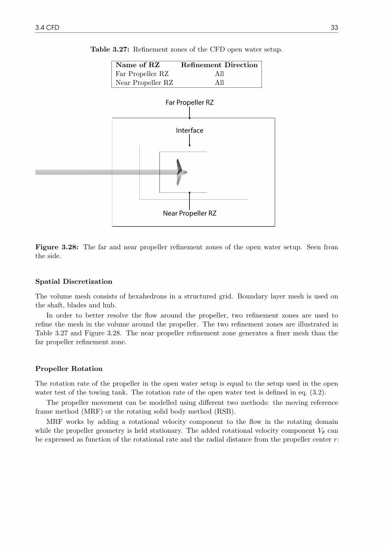
3.4 CFD 33

Table 3.27: Refinement zones of the CFD open water setup.

Name of RZ Refinement DirectionFar Propeller RZ AllNear Propeller RZ All

Far Propeller RZ

Near Propeller RZ

Interface

Figure 3.28: The far and near propeller refinement zones of the open water setup. Seen fromthe side.

Spatial Discretization

The volume mesh consists of hexahedrons in a structured grid. Boundary layer mesh is used onthe shaft, blades and hub.

In order to better resolve the flow around the propeller, two refinement zones are used torefine the mesh in the volume around the propeller. The two refinement zones are illustrated inTable 3.27 and Figure 3.28. The near propeller refinement zone generates a finer mesh than thefar propeller refinement zone.

Propeller Rotation

The rotation rate of the propeller in the open water setup is equal to the setup used in the openwater test of the towing tank. The rotation rate of the open water test is defined in eq. (3.2).

The propeller movement can be modelled using different two methods: the moving referenceframe method (MRF) or the rotating solid body method (RSB).

MRF works by adding a rotational velocity component to the flow in the rotating domainwhile the propeller geometry is held stationary. The added rotational velocity component Vθ canbe expressed as function of the rotational rate and the radial distance from the propeller center r:

34 3 Method

Vθ = 2πnr

MRF can be simulated using a steady-state solver and it has a faster convergence compared to therotating solid body method, which requires a transient solver.

RSB works by rotating the propeller geometry in increments at each new time step. Thismethod requires more computational time, but is a better model of the actual propeller physicscompared to the MRF method. The RSB method models the hull-propeller interaction while theMRF model does not.

The two methods can be combined for computational efficiency. The first step in the combi-nation approach is to firstly accelerate the flow using MRF. When the simulation has converged,it is changed to the more precise and computational heavy RSB and continued until it convergesagain. The combination of methods saves a significant amount of computational time.

Both simulations using MRF and the combination approach have been performed. It is con-cluded from the results of these simulations that the increased accuracy of using the combinationof methods is negligible for the open water simulations, compared to using only MRF. Therefore,it is decided only to use MRF for all open water simulations in order to save computational time.

Studies

Two simulation studies have been conducted with the open water setup: a volume mesh convergencestudy and a comparison with the open water test from the towing tank. The results of the openwater simulations can be seen in Section 4.3.2.

3.4.4 CFD Self-Propulsion TestThe following sections present the background for the self-propulsion simulations. The first sectiondescribes the simulations in model scale and it is followed by a section describing the changes madefrom the model scale setup to the full scale setup.

Model Scale Self-Propulsion

This section describes the CFD setup that simulates the calm water self-propulsion test in modelscale. The setup is created by combining the model scale resistance CFD setup (see Section 3.4.2)with the propeller and the open water CFD setup (see Section 3.4.3).

Physics The physics of the self-propulsion setup is similar to the physics of the resistance setup,but some changes are made. For details on the physics models used in this project see Section 2.3.

The setup uses the k - ϵ turbulence model. Based on the experience from DNV-GL, it has beendecided not to model the free surface waves using the VOF model. Experience from DNV-GLshows that including the VOF model in the self-propulsion setup causes large fluctuations in theresistance, thrust and torque signals. The magnitude of these fluctuations is so large that thefluctuations make it difficult to obtain reliable signals.

Without the free surface waves, it is not possible to model the dynamic pitch and heave of theship using the DFBI model. This is because the DFBI model works by balancing the forces acting

3.4 CFD 35

HullTop

Bottom

InletOutlet Port SideStarboard Side

Top

Bottom

Hull

Figure 3.29: Static domain of the self-propulsion setup, with boundary names. Seen fromstarboard side (left) and from the front (right).

Rotating Domain

Figure 3.30: Rotating domain of the self-propulsion setup. Seen from starboard side.

on the ship. Without the free surface waves, the wave forces on the ship are not modelled, andthe DFBI can not correctly balance the forces. Therefore the DFBI model is not included in theself-propulsion setup.

Instead of modelling the dynamic pitch and heave using the DFBI model, the dynamic pitchand heave of the resistance simulations are prescribed to the self-propulsion simulations beforethey are simulated. The influence of the propeller dynamics on the dynamic pitch and heave ofthe ship is neglected by using the dynamic pitch and heave of the resistance simulations insteadof using the DFBI model in the self-propulsion simulations. Neglecting this influence introduces amodelling error which has not been quantified, but is assumed to be smaller than other modellingerrors.

Domain As in the open water setup, the self-propulsion setup uses two domains; a large staticdomain, with a small rotating domain inside. The shape of the static domain is a rectangularcubeoid, and the shape of the rotating domain is a cylinder.

The static domain can be seen in Figure 3.29. The size of the domains can be seen in Table 3.31,and the boundary conditions of the domains can be seen in Table 3.32.

The static domain of the self-propulsion setup includes both the port and starboard sides ofthe domain. This is different from the resistance setup, where only one side is simulated while theopposite side is accounted for using a symmetry plane. The reason for simulating both sides in

36 3 Method

Table 3.31: Domain size of the CFD self-propulsion setup.

Stationary DomainLongitudinal length 5 LPP

Vertical length 3 LPP

Transverse length 3 LPP

Rotating DomainUpstream length 0.11DDownstream length 0.23DDiameter 1.20D

Table 3.32: Boundary conditions of the CFD self-propulsion setup.

Name of Boundary Boundary ConditionInlet Velocity inlet, prescribed with Vm

Bottom Velocity inlet, prescribed with Vm

Outlet Pressure outletTop Symmetry planeStarboard Side Symmetry planePort Side Symmetry planeInterface Wall and internal interfaceHull, Shaft, Blades, Hub No-slip wall

the self-propulsion setup is because propeller flow is unsymmetrical. Therefore, the self-propulsioncalculations are not modelled using a symmetry plane in the center line.

Without the use of the VOF model, the self-propulsion setup only needs to model the waterphase of the flow. Therefore the top of the static domain of the self-propulsion setup is at the freesurface, and is prescribed with a symmetry plane boundary condition.

Removing the free surface waves from the simulations gives rise to another problem. In reality,a stern wave is created by the ship. The stern wave increases the water height above the propeller,fully submerging the propeller even at low draft conditions such as the sea trial condition. Withoutthe free surface waves, the propeller is not fully submerged. In order to fully submerge the propellerin the self-propulsion setup, the free surface is raised approximately 3% of the draft in the sea trialcondition.

Free Surface Correction The decision not to model the free surface waves and to raise thecalm water surface decreases the measured resistance on the ship. In order to compensate for thischange, a free surface correction is performed on the results of the self-propulsion simulations. Thecorrection is performed in two steps. The free surface correction procedure is shown in Figure 3.33.

The first step is to correct for not modelling the free surface waves, which reduces the hullresistance by removing the wave making resistance. The wave making resistance is quantifiedby simulating the resistance setup both with and without the free surface waves. The differencebetween those two results is the wave making resistance:

3.4 CFD 37

RT

RV

RV,SH

Free surface waves

Initial surface height

No free surface waves

Initial surface height

No free surface waves

Raised surface height

Figure 3.33: The three simulation setups of the free surface correction procedure.

RWm = RTm −RV m (3.38)

where RWm is the wave making resistance and RV m is the total resistance without free surfacewaves, also referred to as the viscous resistance.

The second step is to correct for the raised free surface which increases the resistance on the hull,because a larger surface area is submerged. The increase in resistance is quantified by simulatingthe resistance CFD setup both with the initial and the raised surface heights. The differencebetween those two results is the added resistance due to the raised surface ∆RSHm given by:

∆RSHm = RV m,SH −RV m (3.39)

The resistance of the self-propulsion simulations can then be corrected for wave making resis-tance and added resistance due to the raised surface height:

RTm = RV m,SH +RWm −∆RSHm (3.40)

Spatial Discretization The self-propulsion setup uses two separate meshes; one for the station-ary domain and one for the rotating domain around the propeller. Using two separate meshesallows mesh options from the resistance setup to be used for the static domain and mesh optionsfrom the open water setup to be used for the rotating domain.

Four mesh refinement zones are used in the self-propulsion setup. The four refinement zonescan be seen in Table 3.34 and Figure 3.35.

Propeller Rotation Two different methods or a combination of them can be used to model therotation of the propeller. The two methods are the moving reference frame method (MRF) andthe rotating solid body method (RSB). The methods are described in Section 3.4.3.

38 3 Method

Table 3.34: Refinement zones of the CFD self-propulsion setup.

Name of RZ Refinement DirectionBulbous Bow RZ AllTransom RZ AllFar Propeller RZ AllNear Propeller RZ All


Far Propeller RZ

Near Propeller RZ

Figure 3.35: The four refinement zones of the self-propulsion setup. Seen from starboard side.

For the self-propulsion simulations a combination of the two methods is used. The modellingof the propeller rotation is initialized by using the MRF method, followed by the RSB method.

In the self-propulsion tests, a towing force is applied to the model ship, as described in Sec-tion 3.2.3. The CFD self-propulsion setup is carried out using the same principle. The forces onthe model ship must be balanced, which leads to this expression:

RTm = Tm + FD (3.41)

The towing force has been provided by the towing tank and is defined in eq. (3.10). Thecorrected total resistance is calculated from eq. (3.40). The thrust is adjusted by changing thepropeller rotation rate during the simulation until the forces are in balance.

In total, the self-propulsion simulation uses three stages. First, the simulation is initializedusing MRF. Next, the RSB which changes the propeller rotation rate in order to balance theforces is applied. Lastly, the propeller rotation rate is frozen at the force equilibrium and thesimulation is continued using RSB for one whole rotation. The three stages of the self-propulsionsimulation are illustrated in Figure 3.36.

Temporal Discretization The self-propulsion setup requires a transient solver in order to sim-ulate the rotation of the propeller. An unsteady implicit solver with a first-order scheme is used.

3.4 CFD 39

MRF RSBRSBconst rotation rateconst rotation rate variable rotation rate

Figure 3.36: The three stages of the CFD self-propulsion simulations.

Table 3.37: Appendages used in the model scale CFD self-propulsion studies.

Study With Rudder With Stator FinsTime Step Convergence Yes NoVolume Mesh Convergence Yes NoComparison Yes Yes

The choice of time step size is based on the physics of the propeller rotation. The time stepcan therefore be expressed in terms of the number of degrees the propeller rotates between twotime steps:

∆θ = n ·∆t · 360◦ (3.42)

where ∆θ is the angle per time step and ∆t is the time step size.

Studies Three simulation studies have been conducted on the model scale self-propulsion setup.The three studies are: a time step convergence study, a volume mesh convergence study and acomparison with the self-propulsion results from the towing tank. The appendages mounted ineach of the three studies can be seen in Table 3.37.

The results of the model scale self-propulsion studies can be seen in Section 4.3.3.

Full Scale Self-PropulsionThe full scale self-propulsion setup is created by scaling up the model scale self-propulsion setupaccording to the scaling factor (2.3).

Free Surface Correction The free surface correction method is changed slightly from modelscale to full scale in order to account for the roughness resistance, air resistance and bilge keelresistance which are only relevant for the full scale simulations. The method is still conducted byusing the three simulations setups seen in Figure 3.33. The wave making resistance and the addedresistance of the increased surface height are calculated similarly to eq. (3.38) and eq. (3.39):

RWs = RTs −RV s (3.43)

∆RSHs = RV s,SH −RV s (3.44)

40 3 Method

Table 3.38: Appendages used in the full scale CFD self-propulsion studies.

Study With Rudder With Stator FinsTime Step Convergence Yes YesVolume Mesh Convergence Yes YesComparison Yes Yes

The full scale resistance corresponding to eq. (3.20) is then calculated using:

RTs =S + SBK

S(RV s,SH +∆RF ) +RWs +RAAS −∆RSHs (3.45)

where ∆RF is the roughness resistance of eq. (3.21), and RAAS is the air resistance of eq. (3.23).The correlation allowance of eq. (3.22) is not included in eq. (3.45) because its purpose is to correctfor systematic errors in the towing tank extrapolation procedure.

An alternative to using the ITTC procedure to estimate the roughness, air and bilge keelresistances is to model them in the CFD simulations. The roughness resistance can be modelledusing a wall roughness model [28, p. 3405-3406]. The air resistance requires the superstructure ofthe ship as a 3D geometry. If the 3D geometry of the superstructure is available, the air resistancecan be estimated either by including the superstructure directly in the CFD simulations, or byrunning a separate set of simulations with the superstructure alone. The added resistance fromthe bilge keels can quite easily be estimated by adding the bilge keels to the hull geometry.

Propeller Rotation The full scale self-propulsion setup uses the same method as the modelscale setup for modelling the propeller rotation (see Figure 3.36). The force balance used in thefull scale setup is changed slightly from eq. (3.41) because there is no towing force in full scale:

RTs = Ts (3.46)

The thrust is adjusted by changing the propeller rotation rate until the thrust is equal tothe resistance. The adjustments are performed by a proportional controller programmed by theauthors.

Studies The studies conducted on the full scale self-propulsion setup are a time step convergencestudy, a volume mesh convergence study, and a comparison with the extrapolated self-propulsionsimulation from the towing tank. Both the rudder and stator fins are mounted in all full scaleself-propulsion simulations, as seen in Table 3.38.

The results of the full scale self-propulsion simulations can be seen in Section 4.3.3.

CHAPTER 4Results

This chapter presents the results from towing tank tests in Section 3.4 followed by the speed trialresults in Section 3.4. Finally the results from the CFD simulations are presented in Section 4.3.

4.1 Towing Tank TestThe design of the ship has been tested in a towing tank prior to the project period of this thesis. Theconducted tests include resistance test, open water tests and self-propulsion tests. All of the towingtank tests are conducted with rudder and pre-swirl fins mounted and at the sea trial condition. Thesea trial condition has 40.2% of the displacement of the design condition as explained Section 3.1.1.The method behind the towing tank tests and the procedure for extrapolating from model scaleto full scale are presented in Sections 3.2.4 to 3.2.6. The following sections present the providedtowing tank test results and the extrapolated full scale results.

4.1.1 Results of Resistance TestA resistance test has been carried out at the towing tank, as described in Section 3.2.1. Themodel scale total resistance coefficient and the model scale frictional resistance coefficient havebeen provided by the towing tank. The frictional resistance coefficient is based on the Schoenherrfrictional line in eq. (2.13). The residual resistance coefficient is calculated using eq. (3.1). Themodel scale total, frictional and residual resistance coefficients are presented in Figure 4.1.

From Figure 4.1 it is seen that the frictional resistance is the largest part of the total resistancein the studied Froude number range. It is also seen as expected, that the frictional resistancecoefficient becomes smaller as the Froude number and the Reynolds number increases, and thatthe residual resistance coefficient becomes larger.

4.1.2 Results of Open Water TestAn open water test of the stock propeller has been carried out in the towing tank, as describedin Section 3.2.2. Data of the stock propeller can be seen in Table 3.4. The model scale propellercharacteristics of the stock propeller provided by the towing tank are presented in Figure 4.2.

As seen in Figure 4.2 the open water test is only conducted for advance ratios in the rangerelevant for this ship design. Therefore propeller characteristics are not provided in the the bollardpull range or in the range where the open water efficiency decreases.

4.1.3 Results of Self-Propulsion TestA self-propulsion test has been carried out at the towing tank, using the stock propeller. The self-propulsion test is described in Section 3.2.3. Data of the stock propeller is presented in Table 3.4.

42 4 Results

0.14 0.15 0.16 0.17 0.18 0.19 0.20 0.21

Fn [-]

0

2

4

6C

oeffi

cien

ts [-

]×10-3

Figure 4.1: Results of the resistance test from the towing tank. Model scale total resistancecoefficients CTm (circle), frictional resistance coefficients CFm,Sh (square) and residual resistancecoefficients CR (triangle) as a function of Froude number Fn.

0.25 0.30 0.35 0.40 0.45 0.50 0.55 0.60

J [-]

0.1

0.2

0.3

0.4

0.5

0.6

Coe

ffici

ents

[-]

Figure 4.2: Results of the open water test from the towing tank. Propeller thrust coefficientKTom,stock (circle), 10 times torque coefficient 10KQom,stock (diamond) and open water efficiencyηom,stock (square) of the stock propeller in model scale as a function of advance ratio J .

4.1 Towing Tank Test 43

0.14 0.15 0.16 0.17 0.18 0.19 0.20 0.21

Fn [-]

0.22

0.24

0.26

Coe

ffici

ents

[-]

Figure 4.3: Results of the self-propulsion test from the towing tank in model scale. Propellerthrust coefficient KTm (circle) and propeller torque coefficient KQm (square) as a function ofFroude number Fn.

The thrust identity method has been used to derive parts of the self-propulsion results and isexplained briefly in Section 3.2.6 and [5, Sec 8.7.4.3]. The thrust coefficient eq. (3.13) and thetorque coefficient eq. (3.16) is shown in Figure 4.3. It is observed that the thrust and torquecoefficients have a limited dependence on the Froude number.

4.1.4 Extrapolation of Resistance TestThe results of the resistance test shown in Section 4.1.1 are extrapolated to full scale using theITTC extrapolation method [10, Sec. 2.4.1] as explained in Section 3.2.4. The extrapolationis based on the full scale propeller characteristics of the actual propeller. The total resistancecoefficient eq. (3.20), the smooth total resistance coefficient eq. (3.19), the frictional resistancecoefficient eq. (2.12) and the residuary resistance coefficient eq. (3.1) are presented in Figure 4.4.

From Figures 4.1 and 4.4 it is seen that the frictional resistance is still the largest part of thetotal resistance in full scale, but it is a smaller part than in model scale. This means that infull scale, the frictional resistance is less of the total resistance and the wave making resistance(residuary resistance) is more of the total resistance.

4.1.5 Extrapolation of Open Water TestThe open water characteristics of the actual propeller in full scale have been given by the shipyard.Data of the actual propeller can be seen in Table 3.3. However, the open water characteristics ofthe stock propeller provided by the shipyard is in model scale. Data of the stock propeller canbe seen in Table 3.4. In order to compare the actual propeller with the stock propeller, the openwater characteristics of the stock propeller presented in Section 4.1.2 need to be extrapolated. The

44 4 Results

0.14 0.15 0.16 0.17 0.18 0.19 0.20 0.21

Fn [-]

0

1

2

3

4

Coe

ffici

ents

[-]

×10-3

Figure 4.4: Results of the extrapolated resistance test from the towing tank. Full scale totalresistance coefficient CTs (circle), total resistance coefficient with smooth hull and without bilgekeels CTs,smooth (diamond), frictional resistance coefficient CFs (square) and residuary resistancecoefficient CR (triangle) as a function of Froude number Fn. The extrapolation is conducted usingthe standard ITTC extrapolation method.

ITTC procedure for extrapolating open water characteristics is described in Section 3.2.5. Theextrapolated open water characteristics of the stock propeller are compared to the provided openwater characteristics of the actual propeller in Figures 4.5 and 4.6.

A difference between the performance characteristics of the actual and stock propellers can beseen in Figures 4.5 and 4.6. The actual propeller delivers about 1% to 3% more thrust and about4% to 9% more torque than the stock propeller. This results in a lower open water efficiency of theactual propeller of 2% to 6% compared to the stock propeller, as seen in Figure 4.6. It is importantto remember that the percentages are within the expected magnitude of the measurement andextrapolation uncertainties.

4.1.6 Extrapolation of Self-Propulsion TestThe results of the self-propulsion test and the open water test shown in Section 4.1.3 are extrap-olated to full scale using the ITTC extrapolation method [10, Sec. 2.4.3] as explained in theSection 3.2.6.

The extrapolation is done using both the actual propeller characteristics and the extrapolatedstock propeller characteristics. The delivered power of the extrapolated self-propulsion results canbe seen in Figure 4.7.

The extrapolation using the stock propeller predicts a 4− 5% lower delivered power than theextrapolation using the actual propeller. The difference in delivered power between the stockpropeller and the actual propeller is discussed in Section 5.3.

4.1 Towing Tank Test 45

0.25 0.30 0.35 0.40 0.45 0.50 0.55 0.60

J [-]

0.10

0.15

0.20

0.25

0.30

Coe

ffici

ents

[-]

Figure 4.5: Results of the extrapolated open water test from the towing tank. Thrust coeffi-cient KTos,stock (plus sign) and 10 times the torque coefficient 10KQos,stock (triangle) of the stockpropeller as function of advance ratio J . Thrust coefficient KTos,actual (circle) and 10 times thetorque coefficient K10Qos,actual (diamond) of the actual propeller as function of advance ratio J .The extrapolation is conducted using the standard ITTC extrapolation method.

0.25 0.30 0.35 0.40 0.45 0.50 0.55 0.60

J [-]

0.30

0.40

0.50

0.60

0.70

0.80

ηos

[-]

Figure 4.6: Results of the extrapolated open water test from the towing tank. Open waterefficiency ηos,stock of the stock propeller (asterisk) and open water efficiency ηos,actual of the actualpropeller (square) as a function of advance ratio J . The extrapolation is conducted using thestandard ITTC extrapolation method.

46 4 Results

0.14 0.15 0.16 0.17 0.18 0.19 0.20 0.21

Fn [-]

40

60

80

100

120

140

160D

eliv

ered

Pow

er [%

MC

R]

Figure 4.7: Results of the extrapolated self-propulsion test from the towing tank. Deliveredpower PDs in full scale using stock propeller (asterisk) and actual propeller (triangle) as a functionof Froude number Fn. The extrapolation is conducted using the standard ITTC extrapolationmethod.

4.2 Sea TrialThis section presents the results from the speed trial. The results provided by the shipyard are themeasured values corrected for wind and current. The procedures of the sea trial and correctionsare described in Section 3.3.

The weather data shows that only one of the ships has to be corrected for waves using the ISO15016:2015 standard. The relative difference between the uncorrected and the corrected power dueto waves is between 1% and 3.5%. The corrected speed trial data of the four sister ships can beseen in Figure 4.8.

4.3 CFDThe following sections present the results of the CFD simulations. Details on the simulations canbe found in Section 3.4. First, the results of the resistance test are presented followed by theresults of the open water. Finally, the results of the self-propulsion results are presented. The usedcomputational power for calculating one speed for the different test types can be seen in Table 4.9.

4.3.1 CFD Resistance TestThis section presents results of the model scale and full scale resistance setup. First, the modelscale results are presented, and then the full scale results are presented. The model scale and fullscale resistance CFD setups are described in Section 3.4.2.

4.3 CFD 47

Fn [-]0.14 0.15 0.16 0.17 0.18 0.19 0.2 0.21

Del

iver

ed P

ower

[% M

CR

]

50

60

70

80

90

100

Figure 4.8: Results of the speed trial for all four sister ships. Delivered power as a function ofFroude number Fn. Conducted and corrected using the ISO 15016:2015 procedure [4].

Table 4.9: Used computational power for a single simulation. All simulations are performed on16-core nodes (Either Xeon E5-2650 or Xeon E5-2670 running at 2.60 GHz)

Simulation Computational CostResistance 450 CPU hoursOpen water 32 CPU hoursSelf-propulsion 550 CPU hours

Model Scale Resistance

Before trusting the results of the CFD resistance simulations, convergence tests and validation withmodel scale resistance experiments are essential as explained in Section 3.4.1. The following sec-tions present validation and convergence studies of the boundary layer mesh, spacial discretization,temporal discretization and finally a comparison with towing tank test results.

Boundary Layer Mesh The boundary layer mesh is the part of the mesh situated closest tothe hull (See Figure 2.3). The frictional resistance is dependent on the wall y+ value of the hull,which is controlled by the thickness of the inner most boundary layer as explained in Section 2.3.5.A wall y+ study is conducted in order to determine the boundary layer thickness to be used in thesubsequent simulations.

There are multiple ways of defining a representative global y+ value for a simulation. In thisstudy, the global wall y+ value is assumed to be the average wall y+ of all cells on the wettedsurface of the hull.

It has been decided to perform the y+ study at the lowest speed tested in the towing tank,which corresponds to a Froude number equal to 0.1480. The reason for performing the study at

48 4 Results

0 20 40 60 80 100

Average wall y+ [-]

2.6

2.8

3

3.2

3.4

CF

m [-

]

×10-3

Figure 4.10: Results of the wall y+ study in model scale, showing the frictional resistancecoefficient CFm from CFD (circle) as a function of average wall y+ value, together with the ITTCMode-Ship Correlation Line eq. (2.12) (dash line). Simulations are performed at a Froude numberFn equal to 0.1480, using 2M cells.

Table 4.11: Boundary layer settings of the model scale CFD resistance setup, used to achievewall y+ values in the range of 35 to 50.

Number of boundary layers 7Total boundary layer thickness 8.4× 10−3Lpp

boundary layer stretching 1.4

the lowest speed is that the frictional resistance is the largest part of the total resistance at thelowest speed as described in Section 2.1.

The wall y+ study is conducted by running a series of simulations with different values ofboundary layer thickness while keeping all other mesh settings constant. The frictional resistancecoefficients of the series of simulations can be seen in Figure 4.10, along with the ITTC Model-ShipCorrelation Line eq. (2.12).

It is seen in Figure 4.10 that the frictional resistance coefficient converges at a wall y+ valueof approximately 35 to 50, which is expected as the inner cell is in the log layer as described inSection 2.3.5. This range of wall y+ values is achieved by using the boundary layer settings shownin Table 4.11 for all speed.

Spatial Discretization A mesh convergence study is conducted in order to determine the meshsettings of the volume mesh and the six refinement zones. The refinement zones are described inSection 3.4.2.

The mesh convergence study is conducted by running a series of simulations with different meshsettings while all other settings of the simulations are kept constant. Three of these simulationseries are conducted, each at a different Froude number. The three Froude numbers are chosen

4.3 CFD 49

0 0.5 1 1.5 2 2.5 3 3.5 4 4.5

Number of cells [×106]

-3

-2

-1

0

1

Dis

crep

ancy

in C

Tm

[%]

Figure 4.12: Results of the volume mesh convergence study for the model scale resistance setup.Total resistance coefficient CTm of the CFD simulations relative to the results of the towing tankresistance test at three speeds as a function of the number of cells. Froude number Fn equal to0.1634 (circle), Froude number Fn equal to 0.1736 (diamond) and Froude number Fn equal to0.1940 (square).

from the range of Froude numbers used in the towing tank tests. The mesh convergence study isperformed on the hull without the rudder and without the stator fins as seen in Table 3.22.

The results of the three simulations series show that mesh convergence is obtained at themedium and the highest speeds, but not at the lowest speed. The lack of mesh convergence atthe lowest speed is investigated by inspecting the free surface height. It is concluded that the lackof mesh convergence at the lowest speed is caused by insufficient mesh resolution of the Kelvinwave zone in the longitudinal and transverse directions. The Kelvin waves are briefly described inSection 2.1. Lower ship speeds generate divergent waves with shorter wave lengths. Therefore, themesh of the Kelvin waves should be finer in order to properly resolve the waves at all ship speeds.

The settings of the free surface refinement zones are modified with finer mesh in the longitudinaland transverse directions. The results of the mesh convergence study with the modified settingscan be seen in Figure 4.12.

The resistance coefficients of the mesh convergence study are slightly lower than those of thetowing tank results because the rudder and stator fins are not included in the simulations. Theconclusions of the study are still valid as the effect of the rudder and stator fins on the convergenceis assumed to be negligible. Furthermore, it is important to remember that the discrepancies aresimilar to the uncertainties of the measurements from the towing tank [37].

50 4 Results

Table 4.13: Cell sizes of refinement zones in the model scale CFD resistance setup. Cell sizes aremade non-dimensional using eq. (4.1).

Name of RZ Cell Size l∗ [-]Far Free Surface RZ 96Middle Free Surface RZ 192Near Free Surface RZ 384Bulbous Bow RZ 77Transom RZ 128Vertical Free Surface RZ 1281

From Figure 4.12 it is seen that the results are converged at 2M cells, but with lower discrepancyat 3.7M cells. It is decided not to optimize the volume mesh further because most of the resultsare within the uncertainty of the towing tank measurements data [37]. The cell size ∆l is non-dimensionalized using the ship length:

l∗ =Lpp

∆l(4.1)

where l∗ is the non-dimensional cell size. The non-dimensional cell size can be interpreted as thenumber of cells needed to obtain one ship length. Larger values of l∗ indicate smaller cell sizes.

The mesh with 3.7M cells is used for all subsequent resistance simulations in model scale, andthe settings of the refinement zones can be seen in Table 4.13.

Temporal Discretization The CFD setup is simulated using an implicit unsteady solver asdescribed in Section 3.4.2. The size of the time step is determined by conducting a time step study.The time step is non-dimensionalized using the ship speed and ship length:

t∗ = ∆tVdesign

LPP(4.2)

where t∗ is the non-dimensional time step. A physical interpretation of this non-dimensionaltime step is the number of ship lengths the ship translates per time step.

The time step study is conducted by running a series of simulations with different time stepsizes while all other settings are kept constant. The simulation series are conducted using the 3.7Mcell mesh at a Froude number equal to 0.1736. The study is performed on the hull, without therudder and without the stator fins as seen in Table 3.22. The total resistance coefficient of theCFD simulations are compared to the resistance test data from the towing tank. The results ofthe time step study can be seen in Figure 4.14.

The resistance coefficients of the time step study are slightly lower than those of the towingtank results as the rudder and stator fins are not present in the simulation series. The conclusionsof the study are still valid as the effect of the rudder on the convergence is assumed to be negligible.

Figure 4.14 shows that a smaller time step gives a smaller discrepancy between the resistancesof the CFD and the towing tank. As in the mesh convergence study in Section 4.3.1, it importantto keep in mind that the discrepancies are in the same order of magnitude as the uncertainty of the

4.3 CFD 51

0.000 0.002 0.004 0.006 0.008 0.010 0.012

t* [-]

-1.6

-1.4

-1.2

-1.0D

iscr

epan

cy in

CT

m [%

]

Figure 4.14: Results of the time step study of the model scale CFD resistance setup. Total resis-tance coefficient CTm of the CFD simulations relative to the results of the towing tank resistancetest as a function of time step size t∗. The simulations are conducted at a Froude number Fnequal to 0.1736 and with 3.7M cells.

towing tank test [37]. It can be seen in Figure 4.14 that a reduction in time step from the largestto the smallest time step size only reduces the discrepancy by approximately half a percent pointwhile requiring over six times the computational time. In this case, it is a high computing costcompared to the reduction of the discretization error. A time step size of 6.6× 10−3 is determinedto be the right balance between reduced discretization error and computational cost.

Other time step study simulations have also been conducted. The results, which are not in-cluded in the thesis, show that when the number of cells is increased, the impact on the discrepancyof changing the time step size is reduced. This means that increasing the number of cells reducesthe requirement of the time step size in order to obtain similar discrepancies.

For the full scale resistance CFD simulations, the increased cost of a small time step can bereduced by varying the time step size during the simulation. This method is described in detail inSection 4.3.1.

Comparison A series of simulations are conducted using the final model scale resistance setup.The series of simulations are conducted at the same speeds as the resistance test of the towingtank. The setup parameters of the series of simulations can be seen in Tables 4.11 and 4.13. Theseries of simulations are performed on the hull with the rudder, but without the stator fins as seenin Table 3.22.

The discrepancy in the total resistance coefficient between CFD simulation and towing tanktest data at each speed can be seen in Figure 4.15.

The total resistance coefficient estimated using CFD is very similar to the towing tank results.For the speed range of Fn 0.16 to 0.19, which is in the range of the sea trial data, the discrepanciesare within 1%. The discrepancy is within the uncertainty of the towing tank test. Furthermore, itis important to state that the towing tank tests are conducted with fins and the CFD calculations

52 4 Results

0.14 0.15 0.16 0.17 0.18 0.19 0.20

Fn [-]

-2.0

-1.5

-1.0

-0.5

0.0

0.5

Dis

crep

ancy

in C

Tm

[%]

Figure 4.15: Results of the model scale resistance setup. Total resistance coefficient CTm of theCFD simulations relative to the results of the towing tank resistance test as a function of Froudenumber Fn. The simulation series are conducted using a 3.7M cell mesh with a time step size t∗equal to 6.6× 10−3.

are conducted without. Including the fins in the CFD calculations would increase the resistanceslightly.

As additional validation of the resistance setup, the setup has been blind tested on an additionalship. The data were provided by the DNV GL office in Hamburg. The only data provided for thesimulations were the ship geometry, displacement and draft. After a short spatial and temporalconvergence study, the final simulations were performed and the results were sent to Hamburg.The results are not included in this thesis. After the results were received, the Hamburg officeprovided the towing tank test results. The results showed a relative difference in total resistancebelow 1% between CFD and towing tank test. This is the same discrepancy as in the case studiedin this thesis.

With the satisfying convergence studies of both the temporal and spacial discretization andthe very small discrepancies from model tank test in the studied case and in the blind testing, themodel scale resistance setup is considered trustworthy.

Full Scale ResistanceThe setup validated in the previous sections is modified from model to full scale. The followingsections present validation and convergence studies of the spatial and temporal discretization,followed by a comparison with the extrapolated resistance results from the towing tank.

Boundary Layer Mesh A wall y+ study in model scale has been carried out in Section 4.3.1.It has been decided not to study the influence of the y+ value on the frictional resistance in fullscale, but to use the results of the model scale study. It was concluded that wall y+ values in therange of 35 to 50 gives a reasonable estimation of the frictional resistance. Due to the increasesflow velocity in full scale, the number and thickness of the boundary layers have to be changed, in

4.3 CFD 53

Table 4.16: Boundary layer settings of the full scale CFD resistance setup, used to achieve wally+ values in the range of 35 to 50.

Number of boundary layers 15Total boundary layer thickness 7.9× 10−4LPP

boundary layer stretching 1.4

0 1 2 3 4 5 6 7 8


-4

-2

0

2

4

Dis

crep

ancy

in C

Ts,

smoo

th [%

]

Figure 4.17: Results of the volume mesh convergence study for the full scale resistance setup.Total resistance coefficient with smooth hull and without bilge keels CTs,smooth of the CFD simula-tions relative to the extrapolated resistance results of the towing tank as a function of the numberof cells. The simulations are conducted at a Froude number Fn equal to 0.1736.

order to maintain the average wall y+ value. Model scale and full scale boundary layer settingscan be seen in Table 4.11 and Table 4.16 respectively.

Spatial Discretization The volume mesh and refinement zones of the full scale CFD setup aresimilar to those of the model scale setup, as seen in Section 4.3.1. A mesh convergence study of thefull scale setup is conducted by running a series of simulation with different mesh settings whileall other settings are kept constant. The simulation series is conducted on the hull without therudder and without the stator fins (see Table 3.23) and at a Froude number equal to 0.1726. Theresults of the mesh convergence study can be seen in Figure 4.17.

The resistance of the rudder and stator fins are included in the extrapolated resistance data,but not in the CFD setup. This could be one reason for the discrepancies. It is assumed thatthe exclusion of the rudder does not influence the convergence of the study, and therefore theconclusions are still valid.

It is found that the settings of the vertical free surface, bulbous bow and transom refinementzones directly scaled from the model scale simulations are sufficient for properly resolving the fullscale free surface. It is found that the model scale settings of the far, middle and near refinementzones are too coarse and therefore smaller cell sizes in these three zones are used. It has beendecided to use the 4.7M cell mesh for the final full scale simulations. The final cell sizes of the

54 4 Results

Table 4.18: Cell sizes of refinement zones in the full scale CFD resistance setup. Cell sizes aremade non-dimensional using eq. (4.1).

Name of RZ Cell size l∗ [-]Far Free Surface RZ 137Middle Free Surface RZ 275Near Free Surface RZ 549Bulbous Bow RZ 69Transom RZ 92Vertical Free Surface RZ 915

First StageSmall t*

Second StageLarge t*

Third StageMedium t*

Figure 4.19: The three stages of the time step study of the full scale resistance setup.

refinement zones in model and full scale can be seen in Table 4.13 and Table 4.18 respectively. Thecell size is made non-dimensional using eq. (4.1).

Temporal Discretization Similarly to the model scale setup, the full scale setup is simulatedusing an implicit unsteady solver. A time step study has been conducted to determine the timestep size.

The full scale simulations have shown to be quite sensitive to the time step size during thefirst couple of time steps. If the time step size is too large, the simulation experiences numericalinstability, which causes the simulation to break down. The time step size needed to successfullysimulate the first few time steps is very small. Using this time step size throughout the simulationwould require inconveniently large computational effort. Therefore, it has been decided to runthe simulation in three stages, each using a different time step size: Firstly a small time step forinitializing the flow (first stage), then a large time step for fast convergence (second stage), andlastly a medium time step for minimizing the discretization error (third stage). This approachbalances the required computational cost, the numerical instability, and the discretization error.The three stages are illustrated in Figure 4.19.

The time step size of the first stage is chosen purely to avoid numerical instabilities. The timestep sizes of the second and third stages are studied in the time step study. The study is conductedon the hull without the rudder and without the stator fins (see Table 3.23). The results of thestudy are compared to the results of the extrapolated towing tank test. The results of the studycan be seen in Figure 4.20. The time step size is made non-dimensional using eq. (4.2).

The resistance of the rudder and the stator fins are included in the extrapolated towing tankresults, but not in the CFD setup. This gives an offset to the discrepancies. It is assumed that theexclusion of the rudder and stator fins does not influence the convergence behaviour of the study,and therefore the conclusions are still valid.

Simulations with a non-dimensional time step size larger than 0.011 have a very fluctuatingsignal which makes it difficult to compute a reliable time average. The same is true for time stepsizes smaller than 0.0022. This gives a range of stable time step sizes between 0.0022 and 0.011.

4.3 CFD 55

0.000 0.005 0.010 0.015 0.020 0.025 0.030 0.035 0.040

t* [-]

-4.00

-3.50

-3.00

-2.50

-2.00D

iscr

epan

cy in

CT

s,sm

ooth

[%]

Figure 4.20: Results of the time step study of the full scale CFD resistance setup. Total resistancecoefficient with smooth hull and without bilge keels CTs,smooth of the CFD simulations relative tothe extrapolated resistance results of the towing tank as a function of time step size t∗. Thesimulations are conducted at Froude number Fn equal to 0.1712 and with 4.7M cells.

Table 4.21: Time step sizes of the three stages used in the full scale CFD resistance setup.

Stage Time step size t∗ [-]First 7.6× 10−5

Second 1.1× 10−2

Third 2.2× 10−3

The largest time step size in the stable range is chosen for the second stage, and the smallest timestep size in the range is chosen for the third stage. The time step size of the three stages in thefinal setup can be seen in Table 4.21.

Comparison The full scale CFD setup is simulated at all speeds tested in the towing tank andcompared to the extrapolated resistance results of the towing tank. The simulations are performedusing the hull and the rudder, but not the stator fins (see Table 3.23). The setting of the finalsetup can be seen in Tables 4.16, 4.18 and 4.21. The discrepancy in the total resistance coefficientbetween the CFD simulations and the extrapolated resistance results of the towing tank can beseen in Figure 4.22.

From Figure 4.22 it is seen that the total resistance coefficients of the CFD setup is very similarto the extrapolated towing tank results. For the speeds in the range of the sea trial from a Froudenumber of 0.16 to 0.19, the discrepancies are below 1.5 %, which is satisfying since it is about thesame as the uncertainty of towing tank measurements. The discrepancies are also similar to thoseof the model scale setup, as seen in Figure 4.15. Again, the underestimation could be caused bythe fact that the fins are not included in the CFD simulations.

The setup has shown independence of spatial and temporal discretization and small discrepan-cies compared to the extrapolated resistance from the towing tank.

56 4 Results

Fn [-]0.14 0.15 0.16 0.17 0.18 0.19 0.2

Dis

crep

ancy

in C

Ts,

smoo

th [%

]

-3

-2

-1

0

1

Figure 4.22: Results of the full scale resistance setup. Total resistance coefficient with smoothhull and without bilge keels CTs,smooth of the CFD simulations relative to the extrapolated resultsof the towing tank as a function of Froude number Fn. The simulation series are conducted usinga 4.7M cell mesh, with the time step sizes shown in table 4.21.

Table 4.24: Boundary layer mesh settings of the CFD open water setup, used to achieve wall y+values below 1.

Propeller and HubNumber of boundary layers 11Total boundary layer thickness 2.7× 10−3DNear wall boundary layer thickness 3.7× 10−5D

4.3.2 CFD Open Water TestAs described in Section 3.4.1, a validation procedure is required in order to trust the results of theCFD simulations. This section presents the results of the validation for the open water simulationsin model scale.

Boundary Layer Mesh

A number of boundary layers (see Section 2.3.5) are used on the surface of the propeller hub andblades as well as at the boundary between the rotating and stationary domains.

It is decided to fully resolve the boundary layer of the propeller hub and blades. To fully resolvethe boundary layer, the simulations are performed with wall +y values of the propeller blade andhub below 1. A single boundary layer is used on each side of the interface between the static androtating domain in order to make a good alignment of the two domains. The obtained y+ valueson the propeller in open water can be seen in Figure 4.23, and the boundary layer settings can beseen in Table 4.24.

4.3 CFD 57

Figure 4.23: Wall y+ value on the pressure side (left) and suction side (right) of the propellerin the open water setup. Advance ratio is equal to 0.6.

3 4 5 6 7 8 9 10 11 12


-6

-4

-2

0

2

4

Dis

crep

ancy

in K

Tom

[%]

Figure 4.25: Results of the volume mesh convergence study for the open water setup. Thrustcoefficient KTom of the CFD simulations relative to the results of the towing tank open water testas a function of the number of cells. Advance ratio J equal to 0.30 (circle), advance ratio J equalto 0.45 (diamond) and advance ratio J equal to 0.60 (square).

Spacial DiscretizationA mesh convergence study has been conducted in order to determine the volume mesh settingsand the settings of the refinement zones. The mesh convergence study is conducted by running aseries of simulations with different volume mesh settings while all other settings are kept constant.Three simulation series are conducted at J equal to 0.30, 0.45 and 0.60 respectively. The propellercharacteristics of the CFD simulations are compared with the open water test data from the towingtank. The discrepancies of the propeller characteristics are shown in Figures 4.25 to 4.27.

58 4 Results

3 4 5 6 7 8 9 10 11 12


0

1

2

3

4

5

Dis

crep

ancy

in K

Qom

[%]

Figure 4.26: Results of the volume mesh convergence study for the open water setup. Torquecoefficient KQom of the CFD simulations relative to the results of the towing tank open water testas a function of the number of cells. Advance ratio J equal to 0.30 (circle), advance ratio J equalto 0.45 (diamond) and advance ratio J equal to 0.60 (square).

3 4 5 6 7 8 9 10 11 12


-8

-6

-4

-2

0

Dis

crep

ancy

in η

om [%

]

Figure 4.27: Results of the volume mesh convergence study for the open water setup. Openwater efficiency ηomof the CFD simulations relative to the results of the towing tank open watertest as a function of the number of cells. Advance ratio J equal to 0.30 (circle), advance ratio Jequal to 0.45 (diamond) and advance ratio J equal to 0.60 (square).

4.3 CFD 59

Table 4.28: Cell sizes of the refinement zones in the CFD open water setup.

Name of RZ Cell sizeFar Propeller RZ 4.26× 10−2 DNear Propeller RZ 2.13× 10−2 D

0.25 0.30 0.35 0.40 0.45 0.50 0.55 0.60

J [-]

-8

-6

-4

-2

0

2

4

Dis

crep

ancy

[%]

Figure 4.29: Results of the CFD open water test. Thrust coefficient KTom (circle), torquecoefficientKQom (diamond) and efficiency ηom (square) of the stock propeller in open water relativeto the results of the towing tank open water test as a function of advance ratio J .

It can be seen in Figures 4.25 to 4.27 that the solution converges for all advance ratios. It cantherefore be concluded that the propeller characteristics are independent of the mesh size for sizeslarger than approximately 7.5M cells. In all subsequent open water simulations, the mesh with7.5M cells will be used.

Furthermore, it can be seen in the Figures 4.25 to 4.27 that the thrust coefficient is overes-timated by 1 − 2% for J equal to 0.3 and 0.45, and underestimated by 3% for J equal to 0.6,compared to the towing tank test. The torque is overestimated by 3 − 5% for all advance ratios.The open water efficiency is a combination of the thrust and torque coefficients and is thereforeunderestimated by under 3% for J equal to 0.3 and 0.45 and 7% for J equal to 0.6.

The final mesh setting of the open water setup can be seen in Table 4.28.

Comparison

The propeller performance of the stock propeller is calculated with the mesh settings with ap-proximately 7.5M cells. The CFD results compared with the towing tank results can be seen inFigure 4.29.

It can be seen in Figure 4.29 that the discrepancies are reasonable. Generally the torque isoverestimated by 3− 4%. The thrust is overestimated by approximately 2% at the lower advanceratios and underestimated by approximately 2− 4% at the higher advance ratios. This results inan underestimation of the efficiency of up to 7%. There are several possible explanations for the

60 4 Results

Figure 4.30: Flow regimes on the suction side of a propeller blade in model scale, from [38, 39].

discrepancy between the CFD results and the towing tank results seen in Figure 4.29. The propellergeometry used in the CFD setup is slightly different from the stock propeller geometry used inthe towing tank (see Section 3.1.2). This difference could cause discrepancies in the propellercharacteristics. Another explanation for the discrepancy is the turbulence modelling used in theCFD setup. The near wall flow regime on the propeller in model scale is laminar at first andchanges to turbulent somewhere on the blade as illustrated in Figure 4.30.

The CFD simulation in this report enforces turbulent flow in the domain both for model scaleand full scale since the k − ϵ model assumes that the flow is fully turbulent. Therefore, the CFDsetup is not able to model the laminar flow on the propeller. The full scale flow on the propeller isfully turbulent so this possible discrepancy will only occur in model scale. The use of a transitionmodel in the model scale CFD setup has been discussed, but ultimately it has been decided notuse such a model. The use of ordinary turbulence models [40] and transition-sensitive turbulencemodel in analysis of marine propeller performance [41] have been studied in the literature and asensitive in the choice of turbulence model is found. Not implementing a transitional model savesa significant amount of time and it only causes modelling errors in model scale.

4.3.3 CFD Self-Propulsion TestThis section presents the results of the self-propulsion simulations in model scale and full scale.The two setups are presented in Section 3.4.4.

Model Scale Self-Propulsion

The self-propulsion setup is the combination of the full scale resistance setup and the open watersetup, as described in Section 3.4.4. Before the results from the self-propulsion simulations can betrusted, convergence studies of the temporal and spacial discretization must performed. After theconvergence studies, the results of the self-propulsion simulation are compared to the results of

4.3 CFD 61

Figure 4.31: Wall y+ value on the pressure side (left) and suction side (right) of the propeller inself-propulsion simulation at Froude number Fn equal to 0.1736.

the self-propulsion test from the towing tank in order to validate the self-propulsion setup. Thissection presents the results of the convergence studies and the comparison between the CFD andthe towing tank results.

Only the mean value of the signal has been investigated in the convergence studies. Theamplitude and the nature of the signal have not been studied. The time-dependent details of thethrust and torque signal are relevant in e.g. cavitation studies, noise and vibration studies andfatigue fracture studies, but is out of the scope of this thesis. For this thesis, only the time averagedthrust and torque signals are important because only the time-averaged delivered power is neededfor the comparison with the towing tank results.

Boundary Layer Mesh The self-propulsion setup uses the same boundary layer mesh settingas the model scale resistance setup on the hull. The settings can be seen in Table 4.11.

The boundary layer on the propeller in the self-propulsions setup is fully resolved, exactly asit is for the open water setup. Therefore, the simulations are performed with wall y+ values below1, using the same settings as the open water setup. The setting of the boundary layer mesh onthe propeller can be seen in Table 4.24. The wall y+ on the propeller in a self-propulsion test inmodel scale can be seen in Figure 4.31.

It is seen from Figure 4.31 that the wall y+ values are lower than they are in the open watersimulations, as shown in Figure 4.23. This is expected since the velocities are smaller due to thewake of the ship hull. Furthermore, it is seen that most of the cells have a wall y+ below 1 asrequired for fully resolving the boundary layer.

Temporal Discretization A time step convergence study has been conducted in order to deter-mine the time step size of the transient solver. The study has been conducted by running a seriesof simulations with different time step sizes while all other settings of the setup are kept constant.The time step sizes are shown in non-dimensional values using eq. (3.42). The simulation seriesare conducted using a mesh with 10.7M cells in the rotating region and 1.2M cells in the staticregion at a Froude number equal to 0.1736.

62 4 Results

∆ θ [°]0 1 2 3 4 5 6 7

KT

m [-

]

0.184

0.185

0.186

0.187

0.188

Figure 4.32: Results of the time step study for the self-propulsion setup. Thrust coefficient KTm

of the CFD simulations relative to the results of the towing tank self-propulsion test as a functionof time step size ∆theta. The simulations are conducted at a Froude number Fn equal to 0.1736.

∆ θ [°]0 1 2 3 4 5 6 7

KQ

m [-

]

0.025

0.026

0.027

0.028

0.029

Figure 4.33: Results of the time step study for the self-propulsion setup. Torque coefficient KQm

of the CFD simulations relative to the results of the towing tank self-propulsion test as a functionof time step size ∆theta. The simulations are conducted at a Froude number Fn equal to 0.1736.

The study has been conducted on the hull with the rudder, but without the stator fins, asshown in Table 3.37. The simulations has been conducted with the same propeller rotation rate.From the simulation series, the propeller thrust and torque coefficients are obtained. The resultsof the time step study can be seen in Figures 4.32 and 4.33.

In can be seen in Figures 4.32 and 4.33 that the solution in not completely converging in thetemporal discretization. A possible explanation for the lack of convergence could be that the vesselhas a large wake fraction resulting in separation and/or that transient flow structures are present.

4.3 CFD 63

Figure 4.34: Nominal wake field, normalized with the free stream velocity. Result of the modelscale resistance setup including stator fins. Black ring is the propeller diameter. The simulationis conducted at a Froude number Fn equal to 0.1736.

Separation and transient flow structures could be dependent on the temporal discretization andthereby influence the convergence. The nominal wake field can be seen in Figure 4.34.

The time step study simulations are computationally heavy especially at ∆θ equal to 0.5 and1.0. Therefore, is was not possible, with the available computational power, to use time stepssmaller than 0.5∆θ. Even through the solution has not completely converged, the solution is notconsidered to be diverging. It has been decided to perform all further self-propulsion simulationsin model scale with ∆θ equal to 2. This decision is a trade-off between temporal discretizationerror and usage of computational resources.

Spatial Discretization To ensure that the solution is independent of the mesh discretization,a mesh convergence study has been performed. The mesh around the ship has been studied inSection 4.3.1 and the mesh around the propeller in Section 4.3.2. Only settings of the near propellerrefinement zone (see fig. 3.35) are changed in this mesh convergence study as it is assumed that themesh of the static region is sufficiently discretized because it has been validated in Section 4.3.1.

The meshes of the study can be seen in Table 4.35. The simulations have been conducted withthe same propeller rotation rate as the towing tank self-propulsion test, and at the same Froudenumber equal to 0.1736. The simulations have been conducted on the hull with the rudder, butwithout the stator fins, as shown in Table 3.37.

The results of the mesh convergence study show that the difference in thrust and torque betweenall five meshes in Table 4.35 are smaller than the uncertainty of the signals. This is a strongindication that the solution is independent of the mesh discretization. Based on the results of themesh convergence study, it has been decided to use Mesh 1, which is the coarsest mesh, for allfurther simulations. The mesh settings of Mesh 1 can be seen in Table 4.36.

64 4 Results

Table 4.35: Studied meshes of the mesh convergence study, for the model scale CFD self-propulsion setup.

Mesh # Number of cellsMesh 1 6.2MMesh 2 6.6MMesh 3 7.6MMesh 4 9.1MMesh 5 21.2M

Table 4.36: Cell sizes of refinement zones in the model scale CFD self-propulsion setup. Cellsizes are made non-dimensional using eq. (4.1).

Name of RZ Cell size l∗ [-]Bulbous Bow RZ 69Transom RZ 92Name of RZ Cell size [-]Far Propeller RZ 4.26× 10−2DNear Propeller RZ 2.13× 10−2D

Figure 4.37: Separation downstream of the stator fins. From model scale self-propulsion simu-lation at a Froude number equal to 0.1736. The colour indicates the velocity magnitude at r/Requal to 0.5. Seen from starboard side (left), and from port side (right).

Stator Fins A set of self-propulsion simulations have been conducted both with and withoutthe stator fins in order to investigate the performance of the fins and their influence on the flow.The results of the study show that the stator fins significantly improve the performance of thepropeller even though there is significant flow separation on the two fins on starboard side. Theflow around the stator fins can be seen in Figure 4.37.

The study has also shown that the results of the simulations with the stator fins has resulted insmaller discrepancies relative to the towing tank self-propulsion tests, compared to the simulationwithout the stator fins. This is reasonable since the stator fins have also been included in thetowing tank test. It was therefore decided to include the stator fins in all subsequent self-propulsion

4.3 CFD 65

Fn [-]0.14 0.15 0.16 0.17 0.18 0.19 0.2 0.21

Dis

crep

ancy

in n

m [%

]

2

3

4

5

6

7

Figure 4.38: Results of the model scale self-propulsion setup. Propeller rotation rate nm of theCFD simulations relative to the results of the towing tank self-propulsion test as a function ofFroude number Fn.

simulations. It would have been better to conduct all previous simulations, both resistance and self-propulsion, with the stator fins, but unfortunately that has not been possible due to time limitationsof the project. It is important to remember that the resistance simulations conducted prior to theself-propulsion test are mainly meant as validation steps to ensure trustworthy results in the self-propulsion stimulations. When the stator fins are included in the self-propulsion simulations, theinfluence of not having included the stator fins before is very limited.

Comparison This section presents the results from the self-propulsion simulations compared tothe results from the towing tank self-propulsion test. The self-propulsion simulations are conductedat the same Froude numbers as the self-propulsion test from towing towing tank. The series ofsimulations are conducted both with and without the stator fins, as discussed previously.

As described in Section 3.4.4, a solver has been used in order to obtain the correct tow forceby changing the rate of rotation of the propeller. As described in Section 3.4.4, the simulationshave been performed with a variable propeller rotation rate in order to balance the forces andobtain the same towing force as used in the towing tank tests. The obtained towing forces of thesimulations are within 0.4% of the towing force of the towing tank test (calculated using eq. (3.9)).The propeller rotation rate for the balanced solution can be seen in Figure 4.38.

It is seen from Figure 4.38 that the rate of rotation is overestimated in the simulations. Simu-lations have also been conducted without balancing the forces, but using a fixed propeller rotationrate instead. The results are not shown in this thesis. These simulations show an underestimationof the thrust and an overestimation of the resistance compared to the towing tank results. Theover- and underestimation both contribute to an increase in the propeller rotation rate when bal-ancing the forces because the balancing of the forces has been done according to eq. (3.41). Thatexplains why the propeller rotation rate in Figure 4.38 is consistently overestimated.

66 4 Results

Fn [-]0.14 0.15 0.16 0.17 0.18 0.19 0.2 0.21

Dis

crep

ancy

in K

Tm

[%]

-8

-7

-6

-5

-4

-3

Figure 4.39: Results of the model scale self-propulsion setup. Thrust coefficient KTm of the CFDsimulations relative to the results of the towing tank self-propulsion test as a function of Froudenumber Fn.

The thrust coefficient eq. (3.13) of the simulations can be seen in Figure 4.39. The thrust isoverestimated, but the thrust coefficient is underestimated. This is the case because the propellerrotation rate is overestimated, as explained. It can be seen that the magnitude of the thrustdiscrepancy in Figure 4.39 is related to the discrepancy of the propeller rotation rate in Figure 4.38.For the low Froude numbers, the discrepancies are approximately 6− 7% and for the high Froudenumbers the discrepancies are approximately 2− 4%.

The obtained torque coefficients can be seen in Figure 4.40. It is seen that the torque coefficientis overestimated by approximately 6−7% compared to the towing tank results. An overestimationof the torque coefficient is also seen in the open water simulations in Figure 4.29. In the openwater simulations, the overestimation of the torque coefficient is 3− 4%.

Based on the convergence studies and comparisons to the towing tank tests, the results of themodel scale self-propulsion setup are reasonable.

Full Scale Self-PropulsionThe full scale setup is based on the model scale setup validated in the previous section. Themodification from the model scale setup to the full scale setup is described in Section 3.4.4.

In this section, first the changes to the boundary layer are discussed followed by a brief conver-gence study in temporal and spatial descretization. Then the wake field and flows around the statorfins are presented and discussed. Finally, the results from self-propulsion results are presented.

For the full scale simulations, only calculations in the Froude number range of 0.175 to 0.195will be performed. This is the range where the speed trial are conducted and where the modelscale setup shows the smallest discrepancies.

4.3 CFD 67

Fn [-]0.14 0.15 0.16 0.17 0.18 0.19 0.2 0.21

Dis

crep

ancy

in K

Qm

[%]

5

5.5

6

6.5

7

Figure 4.40: Results of the model scale self-propulsion setup. Torque coefficient KQm of theCFD simulations relative to the results of the towing tank self-propulsion test as a function ofFroude number Fn.

Boundary Layer Mesh The wall y+ value on the propeller in the model scale self-propulsionsetup is below 1 as required in order to fully resolve the boundary layer. In the full scale self-propulsion simulations, the Reynolds number is much larger and the boundary layer is muchthinner. It has not been possible to obtain numerically stable full scale simulations using a bound-ary layer mesh with wall y+ values below 1 in full scale. Therefore, it has been decided to usewall y+ values above 30 instead. This way the boundary layer is not resolved, but instead wallfunctions are used to calculate the effects in the boundary layer.

To study the differences of using wall y+ values below 1 and using wall y+ values above30, three model scale self-propulsion simulations have been conducted using wall y+ value above30. The results of these simulations are not included in this thesis, but they are compared to theearlier model scale self-propulsion simulations conducted with wall y+ values below 1. The relativedifference in thrust and torque between the three simulations with wall y+ values above 30, andthe one with wall y+ value below 1 is no larger than 0.5%. This shows that the use of eithervalues below 1 or above 30 has little influence on the thrust and torque results in model scale. Itis assumed that the same is true for the full scale simulations.

Temporal and Spatial Discretization The following convergence studies are performed toensure convergence in the temporal and spatial discretization as described is Section 3.4.1. Thestudies will not be as comprehensive is the case of the resistance, open water and model scaleself-propulsion simulations.

The reason for this is that it is expected that modelling errors contribute more to the uncertaintythan to the discretization errors. The two most significant contributions to the modelling errorsare the use of the stock propeller instead of the actual propeller and that the roughness and airresistance are based on the ITTC procedure and not modelled in the CFD simulations. Therefore,it does not make sense to intensively study the convergence and ensure very small discretization

68 4 Results

Table 4.41: Studied time step sizes of the time step convergence study for the full scale self-propulsion setup.

Time Step # Time Step SizeTime Step 1 1∆θTime Step 2 2∆θTime Step 3 3∆θTime Step 4 4∆θ

Table 4.42: Studied meshes of the mesh convergence study, for the full scale self-propulsion setup.

Mesh # Number of CellsMesh 1 9.6MMesh 2 9.7MMesh 3 9.8MMesh 4 12.0M

errors when the modelling errors is much larger. However, it is still important to ensure that thesetup does not have a high dependence on the spatial and temporal discretization.

For the full scale self-propulsion setup, a time step study has been conducted. The time stepstudy is a slightly smaller version of the study conducted in model scale. The study consists of fourtime step sizes which can be seen in Table 4.41. The time step sizes are shown in non-dimensionalvalues using eq. (3.42). The studies have been conducted at a Froude number equal to 0.1736,using a mesh of 9.8M cells. The studies have been conducted on the hull with both the rudderand stator fins attached, as seen in Table 3.38.

The simulations have been conducted with a constant rate of rotation equal to the rate ofrotation from the extrapolated towing tank tests from eq. (3.31). The relative difference in thrustand torque from these four simulations is smaller than 0.5%. This indicates that the solution isalmost independent of the temporal discretization and that the discretization error is small. It hasbeen decided to use a time step size of 2∆θ, which is the same as in the model scale self-propulsionsimulations.

As described in Section 3.4.4, the mesh is scaled from the model scale to full scale using thescaling factor. A mesh convergence study has been conducted for the full scale self-propulsionsetup. The study is conducted using four different meshes. The meshes of the study can be seenin Table 4.42. The study has been conducted at a Froude number equal to 0.1736. The study hasbeen conducted on the hull with both the rudder and stator fins attached, as seen in Table 3.38.The relative difference in thrust and torque of the simulations in the study are smaller than 1.5%.It is concluded that the meshes give consistent results and that the spacial discretization erroris smaller than the expected modelling error due to the use of the stock propeller instead of theactual propeller. It is decided to use Mesh 3 with 9.8M cells for subsequent simulations. The meshsettings of Mesh 3 are the same as for the model scale self-propulsion simulation, which can beseen in Table 4.43.

Wake field and Stator Fins In the model scale self-propulsion simulations, it was found thatthe stator fins caused separation due to the high angle of attack combined with the significant

4.3 CFD 69

Table 4.43: Cell sizes of refinement zones in the full scale CFD self-propulsion setup. Cell sizesare made non-dimensional using eq. (4.1).

Name of RZ Cell size l∗ [-]Bulbous Bow RZ 69Transom RZ 92Name of RZ Cell size [-]Far Propeller RZ 4.26× 10−2DNear Propeller RZ 2.13× 10−2D

Figure 4.44: Separation downstream of the stator fins. From full scale self-propulsion simulationat a Froude number equal to 0.1736. The color indicates the velocity magnitude at r/R equal to0.5. Seen from starboard side (left), and from port side (right)

wake field. The flow around the stator fins in full scale can be seen in Figure 4.44. It can be seenthat there is almost no separation compared to the flow in model scale seen in Figure 4.37. Asseen in Figure 4.45, the nominal wake field in full scale is much smaller than in model scale. Theincreased water flow to the propeller prevents the stator fins from stalling.

Final Results With the convergence studies performed, the full scale self-propulsion setup isready for the simulations. In these simulations, three stages are used as shown in Figure 3.36.The results of the simulations can be seen in Figure 4.46 where MCR is the maximum continuousrating. The study has been conducted on the hull with both the rudder and stator fins attached,as seen in Table 3.38.

The CFD results will be compared with sea trial data in the next chapter.

70 4 Results

Figure 4.45: Velocity field, normalized with the free stream velocity. Result of the full scaleresistance setup without stator fins. Black ring is the propeller diameter. The simulation isconducted at a Froude number Fn equal to 0.1736.

Fn [-]0.17 0.175 0.18 0.185 0.19 0.195

Del

iver

ed P

ower

[% M

CR

]

60

70

80

90

100

110

120

Figure 4.46: Results of the full scale self-propulsion CFD setup.

CHAPTER 5Discussion

This chapter will discuss the results presented in the previous chapter. Firstly Section 5.1 of thischapter assesses the accuracy of the sea trial results, and the following Section 5.2 compare anddiscuss the results of the extrapolated towing tank results. Finally Section 5.3 is devoted the fullscale CFD simulations.

5.1 Comparison of Sea Trial and In-Service Performance Data

The results from the sea trials presented in Section 4.2 show high correlation between speed andpower, and low scatter of the data points. This indicates that the accuracy of the speed trial datais high. However, there might be systematic errors in the speed trial data. The correction for wind,waves and current is a possible source for systematic errors. As mentioned, the new ISO 15016:2015procedure defines strict standards for conducting sea trials and ensures accurate measurementsand corrections. The power measurements are another possible source for systematic errors. Theconstants of the engine manufacturer formula in eq. (3.34) are approximations. Systematic errorscan not be determined solely from the data provided for this thesis. A way to validate the resultsfrom the sea trial is by comparing the results with performance measurements on the ship afterthe delivery while it is in service.

The ship owner has provided in-service performance data corrected for wind and waves. Thedata is the mean performance of all four sister ships in the first 3-9 months of operation. Thepower is based on torque measurements directly on the shaft and not the engine manufacturerformula as in case of the sea trial measurements. The ship owner has estimated the uncertainty tobe approximately ±3.5% MCR. Uncertainties in the performance data include uncertainties in theraw torque measurement, the correction for wind and waves and the averaging of the data fromthe four sister ships.

The results of the sea trial are compared to the in-service performance data in Figure 5.1. Itcan be seen that the ships use more power during operation than during sea trial. On average,the sea trial data shows 8% less power than the in-service performance data. This is expectedsince the ships are in excellent condition at the sea trial with minimal fouling on the ship hull.Even though both the sea trial data and the in-service performance data have uncertainties, therelatively low offset in power shows that the sea trial data and the in-service performance datameasures delivered power in the same range. As mentioned earlier, there is only a small scatter ofthe sea trial data, which indicates reasonable consistency in the measurements. The combinationof reasonable offset to the in-service data and consistency indicates that the sea trial results havereasonable accuracy. Because the sea trial results are assumed to be accurate, the sea trial resultscan be used as reference for the extrapolated towing tank results and the full scale CFD results.

72 5 Discussion

0.170 0.175 0.180 0.185 0.190 0.195

Fn [-]

60

80

100

120D

eliv

ered

Pow

er [%

MC

R]

Figure 5.1: Comparison of the corrected speed trial results (dot) and the in-service performancedata (dash line). Delivered power PDs as a function of Froude number Fn.

5.2 Comparison of Sea Trial and Towing Tank TestThe sea trial results presented in Section 4.2 are compared to the extrapolated self-propulsionresults from the towing tank test presented in Section 4.1.6. The comparison can be seen inFigure 5.2. By comparing the sea trial and towing tank results directly, it is assumed that thereis no loss in the shaft. Machinery experts at DNV-GL assess that this is a fair assumption sincethere is no gear.

As it can be seen in Figure 5.2, the extrapolated towing tank results give a reasonable goodestimation of the delivered power. The extrapolated towing tank results are overestimating thepower by approximately 3% to 9% with an average of 6% compared to the sea trial results. Con-sidering that towing tank tests are conducted at a much lower Reynolds number and extrapolated,the observed discrepancies are satisfactory. The power overestimation from the towing tank couldindicate that the ITTC procedure gives a conservative estimate of the ship performance.

The towing tank tests are based on measurements which have uncertainties, and the ITTC ex-trapolation procedure also adds uncertainties to the estimation of the full scale ship performance.The accuracy of the ITTC procedure is under constant debate. As an example, recent researchhas questioned the assumption of Reynolds independence of the form factor, as described in Sec-tion 2.2.4. The discrepancies seen in Figure 5.2 show that the ITTC procedure works well in thiscase and that the procedure is a good method for estimating the performance of this ship design.The ITTC procedure has been regularly improved and updated, and is based on over 100 years ofknowledge and experience from towing tanks around the world.

Is it important to remember that the extrapolation of the towing tank results are performed bythe authors using the standard ITTC procedure described in Section 3.2.4. Based on the authorsexperiences, many towing tanks use slightly different coefficients and corrections than the standardITTC procedure recommends. These changes to the standard procedure are based on experience,

5.3 Comparison of Sea Trial and Full Scale CFD 73

0.170 0.175 0.180 0.185 0.190 0.195

Fn [-]

60

80

100

120D

eliv

ered

Pow

er [%

MC

R]

Figure 5.2: Comparison of the corrected speed trial results (dot) and the extrapolated self-propulsion results from the towing tank (triangle). Delivered power PDs as a function of Froudenumber Fn.

tradition, studies of systematic errors and validation studies of each tank. It has not been possibleto have the exact extrapolation procedure that the towing tank uses at our disposal. Therefore,the extrapolation procedure used in this thesis is the standard ITTC procedure.

5.3 Comparison of Sea Trial and Full Scale CFDThe final results of the full scale self-propulsion CFD simulations can be seen in Figure 5.3 togetherwith the extrapolated towing tank results and the sea trial results.

It can be seen in Figure 5.3 that the CFD results are close to the sea trial results. Comparedto the sea trial results, the CFD results overestimates the delivered power by approximately 0% to5% with an average of 2%. It is important to remember that the CFD simulations are performedusing the stock propeller and not the actual propeller. In Section 4.1.6 it is shown that thedelivered power from the extrapolated towing tank tests using the stock propeller characteristicsinstead of the actual propeller characteristics is 4% to 5% lower. This could indicate that the stockpropeller performs slightly better in full scale than the actual propeller. This indication is basedon several assumptions. One assumption is that the ITTC extrapolation procedure of the openwater characteristics is accurate. Research as [34, 42] has questioned the accuracy of the procedure.The comparison is based on open water and self-propulsion tests which both have measurementuncertainties. The origin of the actual propeller characteristics and the method with which it iscalculated is not known to the authors.

It would be interesting to perform CFD simulations with the actual propeller, but it has notbeen possible to get the actual propeller geometry due to confidentiality. Therefore, it is importantto remember that the difference of 4 to 5% is not an accurate value but more an indication that

74 5 Discussion

0.170 0.175 0.180 0.185 0.190 0.195

Fn [-]

60

80

100

120D

eliv

ered

Pow

er [%

MC

R]

Figure 5.3: Comparison of the corrected speed trial results (dot), the extrapolated self-propulsionresults (triangle) from the towing tank and the full scale CFD self-propulsion results (circle).Delivered power PDs as a function of Froude number Fn.

the performance of the stock propeller is similar to or possibly slightly better than the actualpropeller.

Another source of uncertainty is the fact that the roughness resistance on the hull, the airresistance on the super structure and the added bilge keel resistance are all estimated using theITTC procedure (see Section 3.2.4) and not modelled in the CFD simulations. The ITTC procedurefor estimating these resistance contributions has been developed as a part of extrapolating towingtank tests to full scale and is therefore not meant to be used separately for full scale CFD results.By using the procedure on the CFD results, it is expected that uncertainties are introduced. TheITTC procedure estimates that out of the total resistance, the hull roughness is approximately4% to 5%, the air resistance is approximately 3% to 4% and the bilge keels is approximately 1%to 2%. It could have been interesting to model or simulate the hull roughness, air resistance andbilge keels in the CFD simulations. However, due to time constraints, it has been decided not toimplement these elements in the CFD setups.

Prior to this thesis, experts from DNV GL have had discussions with a world leading paintmanufacturer. The paint manufacturer has expressed that a roughness of 150 µm is high. Ahull roughness of 90 µm to 120 µm is a more reasonable estimate. It is noted that the paintmanufacturer is not neutral because they have an interest in estimating a low roughness for theirpaint. Furthermore, it is not known if the roughness given by the paint manufacturer takes weldingseems and anodes into account. However, this could indicate that the roughness resistance whichhas been added to both the towing tank results and the CFD results is too high. As seen inFigure 5.3, both the CFD and towing tank results are overestimating the power. That couldpossibly be explained by an overestimation of hull roughness resistance.

As mentioned in Section 3.4, the CFDmethod simplifies the physics by modelling the turbulencebehaviour instead of resolving the flow. The choice of turbulence model is crucial to the accuracy

5.3 Comparison of Sea Trial and Full Scale CFD 75

of the results. However, by modelling the turbulence, uncertainties are expected. An exampleof a study with different turbulence models in ship hydrodynamics is [3]. Furthermore the freesurface is removed from the self-propulsion simulation and the wave making resistance is estimatedseparately. This modelling error caused by removing the free surface is small based on experiencefrom CFD experts at DNV GL.

Based on the discussion above, the results seen in Figure 5.3 show that the full scale CFDsimulations provides results similar to the sea trials which indicates a great potential for CFDsimulation in predicting the performance of ships. Previously it has not been possible to validatetowing tank results in the fully loaded condition because speed trial data in fully loaded conditionis very rare. The reason for the limited speed trial data is the practicalities related to fully loadthe ship at the speed trial. If full scale CFD is shown trustworthy, CFD simulations can easily beperformed in the fully loaded condition, which is much more interesting than the ballast condition.In order to gain more trust in CFD simulations of self-propelled ships in full scale, more test casesare required. If other cases show results similar to this thesis, it could change the way the maritimeworld predicts the performance of ships in the future.

CHAPTER 6Conclusions

The overall goal of the project has been to develop and validate a CFD model of a full scaleself-propelled ship. This goal has been fulfilled.

The sea trial results of the four sister ships have shown similar performance. A comparison ofthe sea trial results and monitored in-service performance data has shows that the delivered powerin-service is on average approximately 8% higher than the sea trial results. This is expected sincefouling on the hull is present in service but not at the sea trial. The combination of the similarmeasured performance for the sister ships and the reasonable offset to the monitored in-serviceperformance indicates that the sea trial results are a trustworthy reference for the extrapolatedtowing tank data and full scale CFD.

The development of the CFD model has gone through several stages. First a resistance setuphas been validated. The resistance setup has been developed prior to this project. In parallel, anopen water setup has been created and validated. The results of the resistance and open waterCFD calculations have been compared with towing tank results and the results showed smalldiscrepancies of similar magnitude to the measurement uncertainties.

The resistance setup and the open water setup have been combined into a CFD setup thatsimulates a self-propulsion test. First, the self-propulsion test has been simulated in model scale.The results from the model scale self-propulsion simulations have shown reasonable similarity tothe towing tank results.

Based on the model scale setup, self-propulsion test have been simulated in full scale andcompared to sea trial data and the extrapolated self-propulsion test from the towing tank. Thecomparison has shown that the full scale self-propulsion CFD simulations overestimate the deliv-ered power by approximately 2% on average compared to the sea trial results. This discrepancyis reasonable since the simulations have been performed with the stock propeller instead of theactual propeller and the fact that air resistance, bilge keel resistance and hull roughness resistanceare calculated using the ITTC procedure instead of being modelled in CFD.

The provided towing tank test results have been extrapolated to full scale using the ITTCprocedure. It was found that this prediction overestimated the delivered power with 6% in averagecompared to the sea trial results.

The strengths, weaknesses and uncertainties related to the sea trial, CFD and towing tankpredictions have been discussed. This thesis has shown that both the traditional towing tankapproach and full scale CFD can make reasonable estimations of the full scale performance of aship. In the case studied in this thesis, the CFD approach gave an estimation closer to the seatrial results. To conclude whether the full scale CFD or the towing tank approach is superior inprediction of the performance of a ship, more similar studies are required. However, this thesis hasindicated that CFD has great potential to be the method for estimating full scale performance inthe future.

CHAPTER 7Future Work

As mentioned in the conclusion more studies like this are required in order to determine theaccuracy of full scale CFD and extrapolated towing tank tests.

It is recommended for future studies of similar kind, that the availability of and access tokey data (e.g. the ship and propeller geometry, sea trial results, towing tank results) are checkedbefore the project start. A full list of required and optional data can be found in Appendix A. Thedifference in delivered power from sea trial, extrapolated towing tank test and full scale CFD isrelatively small so low uncertainties are required for all data in order to be be able to make strongconclusions.

A disadvantage of the CFD approach is that the turbulence is modelled using a turbulencemodel. Therefore it could be interesting to study the influence of using a different turbulencemodel(e.g. k − ω SST) in the self-propulsion simulations.

Furthermore, it would also be very interesting to include roughness, bilge keel and air resistancein the CFD simulation. Thereby, the CFD approach will be completely independent of the ITTCprocedure.

Bibliography[1] Satu K. Hänninen, Tommi Mikkola, and Jerzy Matusiak. Computational and experimental

study on local ship loads in short and steep waves. Journal of Marine Science and Technology(Japan), 19(1):103–115, 2014.

[2] J. Wackers, B. Koren, H. C. Raven, A. van der Ploeg, A. R. Starke, G. B. Deng, P. Queutey,M. Visonneau, T. Hino, and K. Ohashi. Free-Surface Viscous Flow Solution Methods for ShipHydrodynamics. Archives of Computational Methods in Engineering, 18(1):1–41, 2011.

[3] Lars Larson. Gothenburg 2010, a workshop on numerical ship hydrodynamics.

[4] IMO. ISO 15016:2015. MEPC 68/INF.14, page 1, 2015.

[5] A. Molland, S. Turnock, and D. Hudson. Ship Resistance and Propulsion. Cambridge Univer-sity Press, 2011.

[6] John Newman. Marine Hydrodynamics. MIT Press, 1977.

[7] Milton Van Dyke. An Album of Fluid Motion. 1982.

[8] W. Froude. The Papers of William Froude. 1955.

[9] G. Hughes. Friction and form factor resistance in turbulent flow and a proposed formulationfor use in model and ship correlation. Transactions of the Royal Institution of Naval Architects,96:314–376, 1954.

[10] ITTC. Recommended Procedures and Guidelines, 1978 ITTC Performance Prediction Method,2005.

[11] J. Carlton. Marine Propellers and Propulsion, 3. edition. Butterworth-Heinemann, 2012.

[12] 26th ITTC Resistance Committee. The Resistance Committee, Final Report and Recommen-dations to the 26th ITTC. 26th International Towing Tank Conference, I:17–71, 2011.

[13] L. Eça. On the accuracy of the numerical prediction of scale effects on ship viscous resistance.International Conference on Computational Methods in Marine Engineering, pages 1–10, 2005.

[14] Karl E. Schoenherr. Resistance of flat surfaces. Trans SNAME, pages 40:279–313, 1932.

[15] C. W. B. Grigson. A planar friction algorithm and its use in analysing hull resistance. RINA,1999.

[16] Tahara Y. Katsui T., Asai H., Himeno Y. The Proposal of a New Friction Line. Fifth OsakaColloquium on Advanced CFD Applications to Ship Flow and Hull Form Design, 2005.

82 Bibliography

[17] ITTC. ITTC – Recommended Procedures, Testing and Extrapolation Methods, ResistanceResistance, Test, 7.5-02 -02-01. ReVision, pages 266 – 273, 2002.

[18] A. Garcia-Gomez. On the form factor scale effect. Ocean Engineering, 26(1):97–109, 2000.

[19] D. Park. A study on the effect of flat plate friction resistance on speed performance predictionof full scale. 2015.

[20] Keh S. Min and Seon Hyung Kang. Study on the form factor and full-scale ship resistanceprediction method. Journal of Marine Science and Technology, 15(2):108–118, 2010.

[21] H. C. Raven, A. Van Der Ploeg, A. R. Starke, and L. Eça. Towards a CFD-based predictionof ship performance - progress in predicting full-scale resistance and scale effects. Transac-tions of the Royal Institution of Naval Architects Part A: International Journal of MaritimeEngineering, 150(4):31–42, 2008.

[22] K. Minsaas. Grunnlag for fartsprognoser. Technical report, Marintek (former: Norges Hydro-dynamiske Laboratorier) , Trondheim, Norway., 1982.

[23] D. Wilcox. Turbulence Modelling for CFD, 2nd edition. DCW. Industries, 1998.

[24] Cuong Nguyen. Turbulence Modeling. MIT, 1(8):1–6, 2005.

[25] D. C. Wilcox. Turbulence Modeling for CFD, 3rd edition, 2006.

[26] D. C Wilcox. Formulation of the k-omega Turbulence Model Revisited. AIAA Journal,46(11):2923–3838, 2008.

[27] F. R. Menter. Two-Equation Eddy-Viscosity Turbulence Models for Engineering Applications.American Institute of Aeronautics and Astronautics, 32(8):1989–1605, 1994.

[28] CD-Adapco. STAR-CCM+ Documentation, Version 10.04, 2015.

[29] A.E.P. Veldman. BOUNDARY LAYERS IN FLUID DYNAMICS. Lecture Notes in AppliedMathematics, University of Groningen., 2011.

[30] Salim M. Salim. Wall y+ strategy for dealing with wall-bounded turbulent flows. Proceedingsof the International MultiConference of Engineers and Computer Scientists, II, 2009.

[31] R. Azcueta. Computation of Turbulent Free-Surface Flows Around Ships and Floating Bodies.PhD Thesis, 2001.

[32] ITTC. Recommended Procedures and Guidelines, Testing and Extrapolation Methods Propul-sion, Propulsor Open Water Test, 7.5-02 -03-02.1, 2011.

[33] ITTC. Recommended Procedures and Guidelines, Propulsion/Bollard Pull Test, 7.5-02-03-01.1. – Recommended Procedures and Guidelines, page 16, 2011.

[34] Stephan Helma. An Extrapolation Method Suitable for Scaling of Propellers of any Design.Fourth International Symposium on Marine Propulsors, 2015.

Bibliography 83

[35] Eirik Eisinger. A Method for Describing Ocean Environments for Ship Design. Masters Thesis,University of Oslo, 2016.

[36] Paul Berrisford, D Dee, K Fielding, M Fuentes, P Kallberg, S Kobayashi, and S Uppala. TheERA-Interim Archive. ERA report series, 1(1):1–16, 2009.

[37] M Kume, K. I.; Hirata, N.; Hasegawa, J.; Tsukada, Y.; Hinatsu. Uncertainty Analysis Methodfor Ship Performance Test. Senpaku Gijutsu Kenkyusho Hokoku/papers of Ship ResearchInstitute, 37(5):163–189, 2000.

[38] G. Kuiper. Cavitation inception on ship propeller models. Ph.D. thesis, Delft University ofTechnology, 1981.

[39] Douwe R. Rijpkema, J. Baltazar, and J.A.C. Falcão de Campos. Viscous flow simulationsof propellers in different Reynolds number regimes. Proceedings of the 4th InternationalSymposium on Marine Propulsors, I, 2015.

[40] Ridha Abid. Evaluation of two-equation turbulence models for predicting transitional flows.International Journal of Engineering Science, 31(6):831–840, 1993.

[41] Xiao Wang. Computational Analysis of Marine-Propeller Performance Using Tranition-Sensitive Turbulence Modeling. Journal of Fluid Engineering, 134(1), 2012.

[42] G. Kuiper. The Wageningen Propeller Series, 1992.

APPENDIX ARequired Data

The following is a list of data required to perform a study similar to the study of this thesis.Required data:

• Principal dimensions

• Speed with main engine characteristics

• General arrangement (G/A)

• High quality 3D geometry of hull, rudder, propellers (the one used in model test and actualon ship) and other appendages.

• Exact location of propeller and appendages.

• Full towing tank report with model scale results in sea trial condition. Including results fromresistance test, open water test and self-propulsion. Water temperature at each test. Infor-mation on used corrections to the results (e.g. corrections to the open water characteristics).

• Sea trial report with results corrected for current, wind and waves.

Optional data:

• Sea trial report with raw measurements of speed, rpm, engine power, current, wind andwaves.

• Extrapolated results from a towing tank test.

• 3D geometry of superstructure.

• In-service performance data.

• Added resistance test from towing tank.

• Wind tunnel test report.

DTU Mechanical Engineering

Section of Fluid Mechanics, Coastal and Maritime Engineering

Technical University of Denmark

Nils Koppels Allé, Bld. 403

DK-2800 Kgs. Lyngby

Denmark

Phone (+45) 4525 1360

Fax (+45) 4588 4325

www.mek.dtu.dk

full scale validation of cfd model of self-propelled...

Documents