numerical simulation of the flow in fuel nozzles for...

Numerical Simulation of the Flow in Fuel Nozzles for Two-Stroke diesel Engines

Ma

ste

r T

he

sis

Fredrik Herland AndersenMEK - FM - EP - 2011- 05 July 2011

Fredrik H Andersen

Numerical Simulation of the Flowin Fuel Nozzles for Two-StrokeDiesel Engines

MEK-FM-EP-2011-05

Master Thesis, July, 2011

Numerical Simulation of the Flow in Fuel Nozzles for Two-Stroke Diesel Engines,MEK-FM-EP-2011-05

This report was prepared byFredrik H Andersen

SupervisorsJens Honore Walther (DTU-MEK)Knud Erik Meyer (DTU-MEK)Kristian Mark Ingvorsen(DTU-MEK)Simon Matlok (MAN)Stefan Meyer (MAN)

Release date: Date publishedCategory: 1 (public)

Edition: First

Comments: This report is part of the requirements to achieve the Master ofScience in Engineering (M.Sc.Eng.) at the Technical Universityof Denmark. This report represents 30 ECTS points.

Rights: c©Fredrik Herland Andersen, 2011

Department of Mechanical EngineeringSection of Fluid Mechancis (FM)Technical University of DenmarkNils Koppels AlleBuilding 403DK-2800 Kgs. LyngbyDenmarkwww.mek.dtu.dkTel: (+45) 45 25 19 60Fax: (+45) 45 93 14 75E-mail: [email protected]

Preface

This master thesis is written at the fluid mechanics section at MEK-DTUand in collaboration with MAN Diesel & Turbo in the period of Februaryto July 2011. This aim for this report is to develop a CFD model that isable to model cavitation and then apply this model to a real life fuel injectorprovided by MAN Diesel & Turbo. As far I know this is the first projectwhere internal nozzle flow and cavitation are investigated numerically bothat MEK-DTU and MAN Diesel & Turbo. A second master project thatfocused building up a cavitation test rig and collecting experimental datawas perfomed at MAN Diesel & Turbo parallel to this study. Initially theidea was that the experimental data obtained for that test rig would be usedas benchmark for developing the CFD code used in this study. It was fastdiscovered that the time lines in the two projects did not coincide since itwould take a long time before the test rig would yield data that could beused in this project. The objective was therefore changed to develop a codebased on experimental data for cavitation found in the literature and thenapply this model to a real life fuel injector provided by MAN Diesel & Turbo.

I would like to thank my supervisor Dr. Jens Honore Walther for greatguidance, support and inspiration throughout the project.

Abstract

The fuel injector is a integral component of large two-stoke marine dieselengines as it is responsible for the injection of fuel into the combustionchamber and subsequently influences the combustion process. The fuel in-jector is responsible for the atomization process for the fuel and the presenceof cavitation in the injector nozzles will influence the atomization process.Over the last decades there have been a increasing focus on emission frommarine diesel engines and strong regulations have forced the industry to in-vest in research on how to optimize the fuel consumption and power output.As of today there have not been performed numerical investigation on theinternal nozzle flow and cavittion in the fuel atomizers at MAN Diesel &Turbo and this project will serve as a starting point for investigating thepresence of cavitating flow in fuel injectors.

A CFD model have been developed for cavitation modeling in this study.The cavitation model in this study is based on a homogenous distributionof bubble seeds present in the fluid that grow and collapse by use of theRayleigh-Plesset equation. This is the first project performed at both DTU-MEK and MAN Diesel & Turbo, so the project consists of two phases, adevelopment phase where a numerical model is developed and tuned againstexperimental data from the literature. And a second phase where the nu-merical model is implemented into the real life F0002 fuel injector underoperating conditions. Simulations are performed both for simulations usingconstant pressure boundaries for inlet and outlet and by use of a transientpressure signal for the inlet. A vortex structure is identified inside the SACvolume and by comparing mass flow rates through the nozzle holes and avortex shedding frequency is identified. The flow conditions applied for theF0002 injector showed a supercavitating flow regime.

Contents

List of Figures viii

List of Tables xi

Nomenclature 1

1 Introduction 51.1 Background . . . . . . . . . . . . . . . . . . . . . . . . . . . . 51.2 Thesis statement . . . . . . . . . . . . . . . . . . . . . . . . . 61.3 Non-dimensional numbers and flow coefficients . . . . . . . . 6

2 Theory 92.1 Diesel fuel injector . . . . . . . . . . . . . . . . . . . . . . . . 92.2 Cavitation . . . . . . . . . . . . . . . . . . . . . . . . . . . . . 10

2.2.1 Hydrodynamic Cavitation regimes . . . . . . . . . . . 122.2.2 Vortex Cavitation . . . . . . . . . . . . . . . . . . . . 13

2.3 Bubble dynamics . . . . . . . . . . . . . . . . . . . . . . . . . 142.3.1 Rayleigh Plesset equation . . . . . . . . . . . . . . . . 142.3.2 Bubble equilibrium, growth and collapse . . . . . . . . 18

3 Numerical model 213.1 Introduction . . . . . . . . . . . . . . . . . . . . . . . . . . . . 213.2 Finite Volume Method . . . . . . . . . . . . . . . . . . . . . . 21

3.2.1 Governing equations . . . . . . . . . . . . . . . . . . . 223.2.2 Transient term . . . . . . . . . . . . . . . . . . . . . . 233.2.3 Source term . . . . . . . . . . . . . . . . . . . . . . . . 233.2.4 Convective term . . . . . . . . . . . . . . . . . . . . . 233.2.5 The Diffusive term . . . . . . . . . . . . . . . . . . . . 24

3.3 Segregated Flow Approach . . . . . . . . . . . . . . . . . . . . 253.3.1 SIMPLE Algorithm . . . . . . . . . . . . . . . . . . . 27

3.4 VOF Multi-Phase Model . . . . . . . . . . . . . . . . . . . . . 28

3.5 Cavitation model . . . . . . . . . . . . . . . . . . . . . . . . . 293.6 Turbulence modeling . . . . . . . . . . . . . . . . . . . . . . . 32

3.6.1 k-Epsilon turbulence model . . . . . . . . . . . . . . . 333.7 Boundary Conditions . . . . . . . . . . . . . . . . . . . . . . . 343.8 Subroutines added to the CCM+ Solver . . . . . . . . . . . . 363.9 Alternative numerical models . . . . . . . . . . . . . . . . . . 37

4 Development and tuning of the numerical model 394.1 Winklhofer model . . . . . . . . . . . . . . . . . . . . . . . . . 394.2 Mesh Generation . . . . . . . . . . . . . . . . . . . . . . . . . 424.3 Model parameters . . . . . . . . . . . . . . . . . . . . . . . . 44

4.3.1 Boundary conditions, discretization schemes, turbu-lence spesification and initial conditions . . . . . . . . 44

4.3.2 Fluid properties . . . . . . . . . . . . . . . . . . . . . 454.3.3 Cavitation model parameters . . . . . . . . . . . . . . 464.3.4 Turbulence . . . . . . . . . . . . . . . . . . . . . . . . 52

4.4 Solution Procedure . . . . . . . . . . . . . . . . . . . . . . . . 534.5 Results from the tuned cavitation model . . . . . . . . . . . . 564.6 Investigation of grid dependence . . . . . . . . . . . . . . . . 614.7 Discussion for the model development . . . . . . . . . . . . . 63

5 MAN Diesel F0002 Fuel Injector 675.1 Real life operating conditions . . . . . . . . . . . . . . . . . . 675.2 Initial conditions, time step and boundary conditions . . . . . 695.3 Mesh . . . . . . . . . . . . . . . . . . . . . . . . . . . . . . . . 71

5.3.1 Grid independent solution . . . . . . . . . . . . . . . . 745.4 Convergence problems for continuity equation . . . . . . . . . 75

6 Results 816.1 Introduction . . . . . . . . . . . . . . . . . . . . . . . . . . . . 816.2 Results from the full F0002 geometry without activating the

Cavitation model . . . . . . . . . . . . . . . . . . . . . . . . . 826.2.1 Mass flow and flow parameters . . . . . . . . . . . . . 826.2.2 Flow field Visualization . . . . . . . . . . . . . . . . . 86

6.3 Results from the full F0002 geometry including the Cavitationmodel . . . . . . . . . . . . . . . . . . . . . . . . . . . . . . . 89

6.4 Results from the Full F0002 geometry without activating thecavitation model using a transient pressure input boundarycondition . . . . . . . . . . . . . . . . . . . . . . . . . . . . . 946.4.1 Estimation of Cavitation inception . . . . . . . . . . . 97

7 Discussion and Conclusion 997.1 Discussion . . . . . . . . . . . . . . . . . . . . . . . . . . . . . 997.2 Conclusion and future studies . . . . . . . . . . . . . . . . . . 101

vii

7.2.1 Acknowledgements . . . . . . . . . . . . . . . . . . . . 102

References 103

Appendix 105

A Appendix A 105A.1 Turbulence formulation . . . . . . . . . . . . . . . . . . . . . 105

A.1.1 Two-Layer formulation . . . . . . . . . . . . . . . . . . 105A.1.2 Wall treatment . . . . . . . . . . . . . . . . . . . . . . 107

A.2 Numerical aspects for the cavitation source term . . . . . . . 109

List of Figures

2.1 SAC-type Diesel fuel injector (Dam,2007) . . . . . . . . . . . 92.2 Principle sketch of sac volume and needle (Martynov,2005) . 102.3 Schematic diagram of phase change for water (Franc,2006) . . 102.4 The venturi principle . . . . . . . . . . . . . . . . . . . . . . . 112.5 Relation between the cavitation number CN and the length

of the cavitation region. (Martynov,2005) . . . . . . . . . . . 122.6 Sketch of nozzle entrance that show cavitation inception (Mar-

tynov,2005) . . . . . . . . . . . . . . . . . . . . . . . . . . . . 132.7 Examples of vortex cavitation . . . . . . . . . . . . . . . . . . 142.8 Spherical bubble in an infinite liquid (Brennen,1995) . . . . . 152.9 Part of bubble surface to show force balance (Brennen,1995) . 172.10 Radius of equilibrium of a microbubble as a function of ex-

ternal pressure (Franc,2006) . . . . . . . . . . . . . . . . . . . 19

3.1 Control volume associated with the node P (Martynov,2005) 223.2 Example of spatial distribution of bubble seeds in a liquid

(User guide, 2010) . . . . . . . . . . . . . . . . . . . . . . . . 293.3 bubble growth rate calculated for an arbitrary pressure series

p∞ . . . . . . . . . . . . . . . . . . . . . . . . . . . . . . . . . 313.4 Inlet and outlet shown on the mesh of the MAN Diesel Fuel

Nozzle . . . . . . . . . . . . . . . . . . . . . . . . . . . . . . . 35

4.1 View of the transparent ”two dimensional” nozzle used for theexperiments (Karrholm,2007) . . . . . . . . . . . . . . . . . . 40

4.2 Dimensions of the geometry used in this study . . . . . . . . 404.3 Massflow and corresponding cavitation regimes (Winklhofer

et al. (2001) . . . . . . . . . . . . . . . . . . . . . . . . . . . . 424.4 The computational grid used in the validation process . . . . 434.5 The dp = 85 bar supercavitation regimes of Winklhofer and

Karrholm (Karrholm,2007) . . . . . . . . . . . . . . . . . . . 49

x LIST OF FIGURES

4.6 Distribution of cavitation using hydroscaled values for seeddistribution and radius, dp = 85bar . . . . . . . . . . . . . . . 49

4.7 Distribution of cavitation and velocity usingR0 = 0.5µm,n0 =1.9 · 1013 1/m3 and α0 = 1 · 10−5, CN = 5.68 . . . . . . . . . 50

4.8 Distribution of cavitation using R0 = 0.01061µm,n0 = 2 ·1018 1/m3 and α0 = 1 · 10−5, CN = 5.68 . . . . . . . . . . . 51

4.9 Distribution of cavitation when incorporating the turbulentpressure fluctuations . . . . . . . . . . . . . . . . . . . . . . . 53

4.10 Residual monitors for different solution strategies . . . . . . . 544.11 Final distribution of cavitation for dp = 85 bar, CN = 5.68,

Supercavitation . . . . . . . . . . . . . . . . . . . . . . . . . . 554.12 Mass flow versus pressure difference . . . . . . . . . . . . . . 564.13 Discharge coefficient and mass flow compared to the Cavita-

tion number . . . . . . . . . . . . . . . . . . . . . . . . . . . . 584.14 Cavitation regimes for different CN . . . . . . . . . . . . . . . 594.15 Pressure distribution inside the nozzle . . . . . . . . . . . . . 604.16 Cavitation production rates for dp=85bar CN = 5.68 . . . . . 614.17 The refined Winklhofer grid . . . . . . . . . . . . . . . . . . . 614.18 Cavitation field for refined grid, dp = 85 bar, CN = 5.68 . . . 624.19 vector plot of the entire computational domain dp = 85, CN

= 5.68 . . . . . . . . . . . . . . . . . . . . . . . . . . . . . . . 634.20 Simulation using second order upwind discretization for the

segregated flow solver dp = 85, CN = 5.68 . . . . . . . . . . . 644.21 Simulation using pv = 5400 Pa, dp = 85, CN = 5.68 . . . . . 65

5.1 SAC-type Diesel fuel injector (Dam,2007) . . . . . . . . . . . 685.2 Placement of boundaries and planes for data collection . . . . 705.3 Internal volume and preliminary grid for the F0002 geometry 725.4 Modifications to the F0002 geometry . . . . . . . . . . . . . . 735.5 Close up of the SAC volume and the nozzle outlets . . . . . . 735.6 Local refinement zones shown by the volumetric control ap-

plication . . . . . . . . . . . . . . . . . . . . . . . . . . . . . . 745.7 Mass flow for several preliminary computational grids . . . . 755.8 Residuals for the 700K model . . . . . . . . . . . . . . . . . . 765.9 Spatial distribution of the continuity residual where rcontinuity >

1 · 10−4 . . . . . . . . . . . . . . . . . . . . . . . . . . . . . . 775.10 Residual monitor and mass imbalance scalar view for simula-

tion for 500K cells fitted with expansion tubes . . . . . . . . 785.11 The 700K grid . . . . . . . . . . . . . . . . . . . . . . . . . . 79

6.1 Mass flow . . . . . . . . . . . . . . . . . . . . . . . . . . . . . 836.2 Close up of mass flow fluctuations . . . . . . . . . . . . . . . 846.3 Normalized mass flow for individual nozzles . . . . . . . . . . 846.4 Flow coefficients . . . . . . . . . . . . . . . . . . . . . . . . . 85

LIST OF FIGURES xi

6.5 Spatial pressure distribution in F0002 . . . . . . . . . . . . . 866.6 Streamlines showing fluid path through the SAC volume and

the nozzles . . . . . . . . . . . . . . . . . . . . . . . . . . . . 866.7 Streamline and vector field showing fluid path through the

SAC volume and the nozzles . . . . . . . . . . . . . . . . . . . 876.8 Placement of plane used to collect vector field . . . . . . . . . 876.9 Transient behavior of the vortex . . . . . . . . . . . . . . . . 886.10 Mass flow through injector . . . . . . . . . . . . . . . . . . . . 906.11 Change in mass flow

(mcavmno cav

· 100)

when activating the cav-itation model . . . . . . . . . . . . . . . . . . . . . . . . . . . 91

6.12 Volume of Fraction (VOF) . . . . . . . . . . . . . . . . . . . . 916.13 Cross section view of nozzle 3 . . . . . . . . . . . . . . . . . . 926.14 Cavitation production rates

[m3

s

]. . . . . . . . . . . . . . . . 93

6.15 Pressure distribution in the SAC volume . . . . . . . . . . . . 936.16 The transient pressure signal used in the simulations . . . . . 946.17 Mass flow through the nozzles . . . . . . . . . . . . . . . . . . 956.18 Flow coefficients for the transient simulation . . . . . . . . . . 966.19 Local pressure and placement of probes . . . . . . . . . . . . 97

xii LIST OF FIGURES

List of Tables

3.1 Model coefficients for the standard k-epsilon model . . . . . . 34

4.1 Dimensions for the geometry used in this study . . . . . . . . 404.2 Physical properties of Diesel Fuel . . . . . . . . . . . . . . . . 464.3 Typical values for the cavitation model (Giannadakis,2005) . 474.4 The final parameters for the cavitation model . . . . . . . . . 514.5 Parameters for the cavitation model . . . . . . . . . . . . . . 62

5.1 Model pressure boundaries for the constant boundary simu-lations . . . . . . . . . . . . . . . . . . . . . . . . . . . . . . . 69

5.2 Maximum mass imbalance values for the 700K and 1160K grids 77

6.1 Frequencies and Strouhal numbers for the nozzles . . . . . . . 836.2 Frequency and Strouhal number for the vortex structure . . . 896.3 Frequencies and Strouhal numbers for the nozzles for the sim-

ulation using a transient pressure input boundary . . . . . . . 96

xiv LIST OF TABLES

Nomenclature

Abbreviations

CFD Computational Fluid Dynamics

CFD Semi Implicit Method for Pressure Linked Equations

VOF Volume of fluid

Non-Dimensional numbers

CN Cavitation Number

CN Cavitation number unitless

αv Volume fraction vapor

Greek symbols

ρv Vapor density kgm3

ρl Liquid density kgm3

µ Dynamic viscosity Pa · s

ρ Density kgm3

υ Kinematic viscosity m2

s

Γ Diffusivity

∇ Gradient Operator

ω Under relaxation factor

φ Scalar quantity

φ Turbulent kinetic energy

2 LIST OF TABLES

τ Non-dimensional time

Latin symbols

~a Area vector

f face

n0 Initial seed density 1m

Scav cavitation source term

K Constant

m′

Mass flow correction

pB Bubble Pressure Pa

pg Gas Pressure Pa

pv Critical Pressure Pa

pinlet Inlet Pressure Pa

pinlet Pressure at inlet Pa

poutlet Outlet Pressure Pa

poutlet Pressure at outlet Pa

p Pressure Pa

pv Vapor Pressure Pa

p∞ Ambient Pressure Pa

pv Vapor Pressure Pa

R Bubble radius m

R0 Initial bubble radius m

Rc Critical bubble radius m

m Mass flow rate Kgs

S Surface tension Nm2

u Velocity ms

~p∗ Uncorrected pressure pa

~p′

Pressure correction Pa

LIST OF TABLES 3

~v∗ Uncorrected velocity ms

~v′

Velocity correction ms

v Velocity ms

r radius m

t time s

4 LIST OF TABLES

Chapter 1

Introduction

In the current study a numerical model is developed to model cavitationin fuel nozzles. In this chapter the background for the project is presentedalong with a declaration of some of the non-dimensional parameters andcoefficient used later in the report. Chapter 2 is at theory chapter wheresome fundamentals of cavitation is presented along with a derivation of theRayleigh-Plesset equation, which is the equation that the cavitation model inthis study is based on. The numerical model used in this study is presented inchapter 3. Chapter 4 is dedicated to the model development where the modelparameters and the solution strategy is presented. When the numericalmodel was developed it was applied to a real life fuel injector, namely theF0002 injector provided by MAN Diesel & Turbo, the development of thismodel is presented in chapter 5. The results are presented in chapter 6 anda discussion and conclusion is presented in chapter 7.

1.1 Background

Ever since the inception of the internal combustion engine, scientists andengine builders have tried to optimize the combustion process to maximizepower outlet and minimize fuel consumption. Over the years as the environ-mental consciousness have grown there have been a lot of fucus on reducingthe emission of hazardous gases from the internal combustion engine. Theautomotive industry have been subjected to emission regulations for sev-eral decades and new agreements have already been made for even tighterregulations in the future. This have in turn forced the industry to investin research towards new technology to comply with the future regulations.Due to high costs and a high level of practical complications, the research

6 Introduction

on large two stroke diesel engines lack behind the automotive engines. Theshear size of a large two stroke engine makes experimental work difficult, notto mention the cost involved with building, planning and operating full scaletest facilities. The market for large two stroke engines is also significantlysmaller than for automotive engines so the financial resources available forresearch is smaller.

There are numerous ways of optimizing the combustion process in largetwo stroke diesel engines e.g timing of the exhaust valve, massflow throughthe scavenging ports, various after treatment, optimizing fuel valve and noz-zle configurations and injection timing. The scope of this study is to investi-gate the internal flow in the diesel fuel injector upstream the spray especiallyinvestigating the flow at cavitating conditions as this is believed to have greatinfluence on the spray and subsequently the atomization process.

1.2 Thesis statement

The main purpose of this project is to develop and tune a CFD code capa-ble of modeling cavitation and then apply this model to a real life operatingcondition in a full scale fuel injector called F0002 provided by MAN Diesel& Turbo. This is the first project conducted at MEK-DTU concerning nu-merical modeling of cavitation so subsequently a lot of time was spent ondeveloping and tuning the model parameters for the cavitation model andobtaining a solution strategy. When the cavitation model was obtained itwas implemented in a full scale injector to give a preliminary estimation ofthe cavitation regimes present at operating conditions. The purpose of thisstudy is to gain knowledge of the internal flow conditions in a fuel injec-tor and to investigate the presence of cavitation as this is expected to havedownstream effects on the fuel spray. Providing a tool that provide betterunderstanding of the flow conditions inside the fuel injectors opens up forpossibilities in nozzle design and a better fuel consumption.

This study only concerns with the flow upstream of the nozzle outlet andthere will be no coupling of the flow fields observed in this study and thesubsequent spray.

1.3 Non-dimensional numbers and flow coefficients

Non-dimensional numbers and discharge coefficients are used in this reportto characterize flow regimes at different operating conditions and to stan-dardize the output when post processing results from simulations.

The Reynolds number gives a measure of the ratio of inertial forces toviscous forces and is a key parameter when characterizing flow regimes as

1.3 Non-dimensional numbers and flow coefficients 7

the ratio of inertial to viscous forces denotes the degree of turbulence in theflow. The Reynolds number is written as

Re =ρUbD

µ(1.1)

Where ρ is the density of the fluid, Ub is the mean flow velocity, µ is thedynamic viscosity of the fluid and D is the characteristic length for theflow equal to the diameter for duct flows. If nothing else is stated the bulkvelocity is estimated by a theoretical Bernoulli type velocity scale Ub definedlike

Ub =√

2ρ

∆p (1.2)

where ∆p is the driving pressure difference for the flow. All simulation inthis study is pressure driven so ∆p = pinlet − poutlet.

Vortex structures are likely to occur in internal flow for fuel injectors andsubsequently a shedding frequency is likely to be detected. To normalizethe frequencies the Strouhal number is applied. The Strouhal number is adimensionless number used to describe the oscillating mechanism of vortexshedding and is given by the following expression

St =fL

Ub(1.3)

Where f is the vortex shedding frequency and Ub andL is the velocity andlength scale as for the Reynolds number.

Due to the high pressures and subsequent velocities inside fuel injectorsthe compressibility must be taken into consideration. For this report theMach number is used to determine if compressible effects should be includedin the simulations. The Mach number is the ratio between the free streamvelocity ,U∞, and the speed of sound ,c, for the fluid.

M =U∞c

(1.4)

The Mach number is given by equation (1.4) and the rule of thumb is thatcompressible effects should be included if M > 0.3.

To evaluate the mass and momentum though the ducts the dischargecoefficient and momentum coefficient are applied. The discharge coefficientis the ratio of the actual mass flow though to the theoretical mass flowthrough a orifice

Cd =mactual

mtheoretical=

m

A0ρUb(1.5)

8 Introduction

where A0 is the original cross sectional area of the orifice. The momentumcoefficient is the ratio of momentum flow to the theoretical momentum flow

Cm =Mactual

Mtheoretical

(1.6)

The actual momentum flow rate is found by extracting an area averagevelocity Uavg from a plane in the simulation domain and calculating theactual momentum flow rate manually, equation 1.6 is then written

Cm =A0ρU

2avg

A0ρU2b

=U2avg

U2b

(1.7)

Uavg is calculated from the mass flow like

Uavg =m

A0ρ

Chapter 2

Theory

2.1 Diesel fuel injector

The diesel fuel injector is a integral part of the diesel engine as it injects thefuel into the compressed air in the combustion chamber. It is also responsiblefor the fuel atomization, which for engines running by the diesel principlehas a major influence on the combustion process and directly effects thepower outlet, fuel consumption and emissions.

Figure 2.1: SAC-type Diesel fuel injector (Dam,2007)

Figure 2.1 show a SAC type fuel injector atomizer as the one mountedon MAN Diesel & Turbo‘s engines. Fuel is delivered to the nozzle from asupply pump with supply pressure at approximately 800 bars in the pointmarked ”Head” on the left hand side of figure 2.1. Further downstream thereis a valve that opens at 350 bars giving the fuel a clear path trough the sacvolume and out the nozzle holes.

Figure 2.2 is a close up to the nozzle and shows the needle, sac volumeand nozzle hole. The aim for this project is to investigate the flow field in

10 Theory

Figure 2.2: Principle sketch of sac volume and needle (Martynov,2005)

this region of the atomizer as it is here cavitation is most likely to occur.

2.2 Cavitation

Cavitation is commonly known as the process of formation of vapor dropletsin a liquid created by a sudden drop in the local pressure below the saturationpressure for the liquid. When the local tension pv − p exceeds the tensilestrength of the liquid pv − pcr the fluid surface rupture and yields a smallvoid which serves as a nuclei for the phase transition process [4]. The liquidwill then vaporize in these cavities and bubbles containing vaporized gas willform in the liquid. Other sources of nuclei is non condensable gas, typicallyair, who to some extent is present in fluids in most practical applications.

Figure 2.3: Schematic diagram of phase change for water (Franc,2006)

2.2 Cavitation 11

Since the density of vapor phase is assumed much smaller than the liquidphase the amount of heat consumed locally for the evaporation is negligiblethe process can be assumed isothermal. This is illustrated in figure 2.3 whichshows a schematic diagram of the phase change of water. It shows thatalthough cavitation and boiling share the same phase change the physicalphenomenon is completely different. For boiling the driving phenomenon is abarotropic change in temperature while cavitation is caused by a isothermalchange in pressure.

Cavitation is known to occur in many industrial applications like hy-drodynamical systems, turbopumps, on the trailing edge of a propeller andin diesel injection nozzles. Cavitation in all these examples are the resultof a sudden change in the velocity due to changes in geometry. This isunderstood by use of the Bernouilli equation:

P +12ρV 2 = constant (2.1)

The Bernouilli equation gives the relation between the static and dy-namic pressure. Figure 2.4 shows the a Venturi where the fluid is acceleratedthrough the contraction subsequently yielding a pressure drop as indicated.If the local pressure in the contraction falls below the vapor pressure of theliquid cavitation occurs.

Figure 2.4: The venturi principle

12 Theory

2.2.1 Hydrodynamic Cavitation regimes

The flow conditions described in section 2.2.1 corresponds to hydrodynamiccavitation. Hydrodynamic cavitation is generated when the local pressuredecrease is caused by the hydrodynamic motion of the fluid. To describethe nature of the cavitating flow the cavitation number is applied. Thecavitation number relates the pressure drop to the local static pressures.There are several definitions of the cavitation number, but for this thesisthe following version is found appropriate [7]

CN =pinlet − poutletpoutlet − Pv

(2.2)

Where pinlet and poutlet is the system pressure at the inlet and outlet respec-tively and pv is the vapor pressure of the fluid, usually pv is the same as thesaturation pressure for the given temperature. The cavitation number is adimensionless scalar for cavitation used to indicate the cavitating nature ofthe flow. The cavitation number is not a independent scalar for cavitationas it is geometry dependent but several experimental works have shown arelationship between the cavitation number and the extent of the cavitationregion [7],[17].

Super-cavitation

Transitional cavitation

Sub-cavitation

Cavitation inception

1superCN − -1

incCN -1CN 0

0

L

cavL

Figure 2.5: Relation between the cavitation number CN and the length of thecavitation region. (Martynov,2005)

Figure 2.5 shows a relation between the cavitation number and the averagelength of the cavitating region Lcav. The figure includes the names proposedby Saito and Sato (2001) [15], namely

• Cavitation inception

2.2 Cavitation 13

• Sub-cavitation

• Transitional cavitation

• Supercavitation

Cavitation inception is when cavitation fist occurs in the system. This istypically at the nozzle entrance or in the region immediately adjacent tothe vena contracta. Sub-cavitation stage is when the cavitation regions fillsthe recirculation region located at the entrance of the nozzle. Transitionalcavitation is when the cavitation region stretches further downstream thenozzle. When the length of the cavitation region stretches throughout theentire nozzle region the regime is called supercavitation. When the flowexperiences supercavitation the flow ”chokes” and the mass flow becomesindependent from any increase in pressure difference this point is called”critical cavitation”.

1A

AcA

Nozzle wall Liquid with nuclei

Vapor

Reattachment point

Separation point L

cavL

Vena contractasepL

21

Figure 2.6: Sketch of nozzle entrance that show cavitation inception (Mar-tynov,2005)

2.2.2 Vortex Cavitation

Cavitation can also occur in vortex structures in a flow. Due to centrifugalforces the pressure in the core of the vortex is lower than the pressure faraway from the core and if pv > p, cavitation is expected to occur in thecenter of the vortex flow.

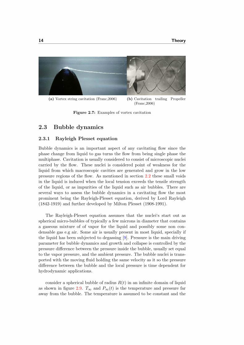
Figure 2.7a shows a known configuration of a three dimensional hydrofoilwhere the pressure difference between the pressure side and the suction sidegenerates a secondary flow which goes around the tip of the hydrofoil andyields a vortex string attached to the top. If the local pressure drops belowthe vapor pressure for the liquid cavitation bubbles form. This phenomenonis very common on the trailing edge of ship propellers as shown in figure 2.7b.

Vortex string cavitation is also likely to occur in diesel fuel injectors sincevortices is likely to form in the SAC volume of the nozzles.

14 Theory

(a) Vortex string cavitation (Franc,2006) (b) Cavitation trailing Propeller(Franc,2006)

Figure 2.7: Examples of vortex cavitation

2.3 Bubble dynamics

2.3.1 Rayleigh Plesset equation

Bubble dynamics is an important aspect of any cavitating flow since thephase change from liquid to gas turns the flow from being single phase themultiphase. Cavitation is usually considered to consist of microscopic nucleicarried by the flow. These nuclei is considered point of weakness for theliquid from which macroscopic cavities are generated and grow in the lowpressure regions of the flow. As mentioned in section 2.2 these small voidsin the liquid is induced when the local tension exceeds the tensile strengthof the liquid, or as impurities of the liquid such as air bubbles. There areseveral ways to assess the bubble dynamics in a cavitating flow the mostprominent being the Rayleigh-Plesset equation, derived by Lord Rayleigh(1842-1919) and further developed by Milton Plesset (1908-1991).

The Rayleigh-Plesset equation assumes that the nuclei‘s start out asspherical micro-bubbles of typically a few microns in diameter that containsa gaseous mixture of of vapor for the liquid and possibly some non con-densable gas e.g air. Some air is usually present in most liquid, specially ifthe liquid has been subjected to degassing [9]. Pressure is the main drivingparameter for bubble dynamics and growth and collapse is controlled by thepressure difference between the pressure inside the bubble, usually set equalto the vapor pressure, and the ambient pressure. The bubble nuclei is trans-ported with the moving fluid holding the same velocity as it so the pressuredifference between the bubble and the local pressure is time dependent forhydrodynamic applications.

consider a spherical bubble of radius R(t) in an infinite domain of liquidas shown in figure 2.9. T∞ and P∞(t) is the temperature and pressure faraway from the bubble. The temperature is assumed to be constant and the

2.3 Bubble dynamics 15

Figure 2.8: Spherical bubble in an infinite liquid (Brennen,1995)

ambient pressure P∞(t) is a known input that controls the growth and col-lapse of the bubble. The collapse of a bubble is known to happen really fastand could produce high local Mach numbers and even shock waves, howeverfor simplicity this derivation assumes the process to be incompressible, whichis valid for most of the process except the final stages of collapse. Further itis assumed that the temperature TB(t) and pressure PB(t) inside the bubbleis constant at all time. The radius of the bubble R(t) is the primary resultof the analysis so parameters will be functions of position from the centerof the droplet and time. Conservation of mass requires that

u(r, t) =F (t)r2

(2.3)

where F (t) is related to R(t) by a kinematic boundary condition at thebubble surface. For the idealized case of zero mass transport across thebubble boundary, it is clear that u(R, t) = dR

dt and hence

F (t) = R2dR

dt(2.4)

This is a good approximation even if there is massflow over the boundary[4]. Volume rate of production of vapor is equal to the rate of increase ofbubble volume

4πR2dR

dt

[m3

s

]and therefore the mass rate of evaporation.

ρv(TB)4πR2dR

dt

[Kg

s

]

16 Theory

This must equal the massflow of liquid inward relative to the interface. In-ward velocity is given by

ρv(TB)ρL

dR

dt

and therefore the velocity can be written

u(R, t) =dR

dt− ρv(TB)

ρL

dR

dt=[1− ρv(TB)

ρL

]dR

dt(2.5)

and by the relation (2.3) and since r ≈ R (2.5) can be written

F (t) =[1− ρv(TB)

ρL

]R2dR

dt(2.6)

In most practical cases the density for the vapor phase is much smallerthan the density for the liquid phase and the approximate form of equation(2.3) is adequate. For Newtonian liquids, the Navier-Stokes equations formotion in the r direction.

−1r

∂p

∂r=∂u

∂r+ u

∂u

∂r− υL

[1r

∂

∂r(r2∂u

∂r)− 2u

r2

](2.7)

substituting u according to equation (2.4)

−1r

∂p

∂r=

1r2

dF

dt− 2F 2

r5(2.8)

Note that the viscous term the Navier-Stokes equation vanishes. In factthe only viscous contribution in the full Rayleigh-Plesset equation comesfrom the dynamic boundary condition at the bubble surface. Applying thecondition p→ p∞ as r →∞ equation (2.8) can be integrated to give

p− p∞ρL

=1r

dF

dt− 1

2F 2

r4(2.9)

A dynamic boundary condition on the bubble surface must be con-structed. Considering a small, infinitely thin lamina containing a segmentof the interface, see figure 2.9. The net force on this lamina in the radiallyoutward direction per unit area is

(σrr)r=R + pB −2SR

(2.10)

Where S is the surface tension of at the bubble interface. since

(σrr)r=R = −p+ 2µL∂u

∂r

the net force per unit area is

pB − (p)r=R −4µLR

dR

dt− 2S

R(2.11)


Figure 2.9: Part of bubble surface to show force balance (Brennen,1995)

In the absence of mass transport across the boundary this force must bezero, and substituting the value for (p)r=R from equation (2.9) with

F = R2dR

dt

yields the generalized Rayleigh-Plesset equation first derived by lord Rayleigh(1917), without the surface tension and viscous contribution, and applied totraveling cavitation bubbles by Plesset (1949) [4]

pB(t)− p∞(t)ρL

= Rd2R

dt2+

32

(dR

dt

)2

+4υLR

dR

dt+

2SρLR

(2.12)

Where pB(t) in most applications are equal to pvapor. This equation canthen be solved for bubble radius as a function of the local pressure p∞. Asone can see, the main driving force to this equation is the pressure differ-ence between the local pressure and the liquid vapor pressure. The equationincludes effects from surface tension and liquid viscosity, but as these con-tributions are inversely proportional to the bubble radius they only havesignificantly influence when the bubble is very small just after growth startand at final stages of collapse. Notice that this model does not include thepresence of any non condensable gas in the vapor bubble and the thermaleffects are neglected.

When the effects of non condensable gas, surface tension and viscosityis negligible which is the case for large enough bubbles the Rayleigh-Plessetequation reduces to the simple Rayleigh equation

Rd2R

dt2+

32dR

dt=pvapor − p∞

ρL(2.13)

18 Theory

which can be integrated once to give the bubble interface velocity(dR

dt

)2

=23pvapor − p∞

ρL

[1−

(R0

R

)3]

(2.14)

Equation (2.14) is the simplified Rayleigh-Plesset equation and yieldsthe asymptotic growth rate for bubble also known as the inertia controlledgrowth model [1]

dR

dt∼=√

23pvapor − p∞

ρL(2.15)

The inertia controlled growth model is the equation used in the cavitationmodel in STAR-CCM+ and will be the basis equation for the cavitationmodeling in this report.

2.3.2 Bubble equilibrium, growth and collapse

After establishing a model for the growth of bubble nuclei it is time toevaluate the equilibrium radius R of a bubble as a function of the liquidpressure p∞. A given nucleus is characterized by a mass of non condensablegas which is assumed constant at any time during the evolution of the bubble.The following equilibrium can be established

pg + pvapor = p∞ +2SR

(2.16)

The evolution of the bubble nuclei is supposed to be isothermal so by use ofthe ideal gas law the pressure of the non condensable gas is inverse propor-tional to the volume of the bubble

pg =K

R3(2.17)

where the constant K is a characteristic of the considered nucleus. equa-tion (2.16) can be rewritten to

K

R3+ pv = p∞ +

2SR

(2.18)

For a given value of K equation (2.18) allows the computation of theequilibrium radius of the nuclei as a function of the external pressure p∞.

Figure 2.10 show the equilibrium curve for a vapor bubble. The solidpart of the line corresponds to stable equilibrium whereas the dotted linecorresponds to when the pressure level is lower than the critical pressureand the bubble grows indefinitely without reaching equilibrium. This meansthat when the local pressure drops below the critical pressure who is notexactly the same, but slightly lower than the vapor pressure, the nucleusbecomes unstable and grow into a macroscopic bubble that travels with the


Figure 2.10: Radius of equilibrium of a microbubble as a function of externalpressure (Franc,2006)

liquid. As mentioned the critical pressure is slightly different to the vaporpressure, this is due to surface tension and the following correlation can beapplied

pc = pvapor −4S3Rc

Rc =

√3pg0R3

0

2S

where Rc is the critical radius where the bubble no longer can obtain equi-librium.

If the local pressure p∞ is lower than the vapor pressure pvapor the bub-ble radius decreases (R < R0). When this happens the bubble collapses.For simplicity the effect of surface tension, viscosity and presence of noncondensable gas are neglected. The Rayleigh-Plesset equation (2.14) is thenwritten

dR

dt∼= −

√√√√23p∞ − pvapor

ρL

[(R0

R

)3

− 1

](2.19)

Equation (2.19) allows the computation of the collapse time for a bub-ble i.e. the time necessary for a bubble of initial radius R0 to completely

20 Theory

disappear (R = 0). This time is called the rayleigh time and is given by [9]

τcollapse ∼= 0.915R0

√ρL

p∞ − pvapor(2.20)

Chapter 3

Numerical model inSTAR-CCM+

3.1 Introduction

This study have been carried out by using the commercial CFD softwareSTAR-CCM+ by CD-Adapco. So the numerical approach by default is theEulerian multi-phase flow with the volume of fluid (VOF) model and theRayleigh-Plesset equation for modeling the phase change. The equationsare solved using the segregated flow solver which solves the flow equations,one for each component of velocity and one for the pressure in a segregatedway. The solution algorithm is the SIMPLE algorithm proposed by Spaldingand Patankar in 1972 [14]. The simulations where turbulence is included ismodeled by use of the standard k-epsilon model. The discretization schemesused in this study is first and second order upwind for the convective termsand the first order temporal discretization scheme for the transient terms.

The mesh was generated by use of the STAR-CCM+ mesh generatingcapabilities. Where neutral IGES files, prepared in Pro-Engineer, is im-ported to the STAR-CCM+ 3D-CAD feature where its surfaces is definedand a volume mesh is generated.

3.2 Finite Volume Method

The finite volume method is a method for representing and evaluating theconservations laws [11] where the solution domain is divided up in a finitenumber of cells on a computational grid. Discrete versions of the integralform of the continuum transport equations are applied to each of the con-

22 Numerical model

trol volumes (cells). The objective is to obtain a linear set of equationscorresponding to the number of cells in the computational domain [1]. Thegrid used in this study is generated using the meshing capabilities in STAR-CCM+. Polyhedral cells with prismatic orthogonal cells in the regions closeto wall boundaries make out the body fitted grid for all simulations in thisstudy. All variables are allocated at the centers of the control volumes.

Figure 3.1: Control volume associated with the node P (Martynov,2005)

Figure 3.1 shows the principle layout of a computational cell in the finitevolume framework where P is the cell node with neighboring nodes E, W ,S, N , L and H and cell faces e, w, s, n, l and h.

3.2.1 Governing equations

The transport of a scalar quantity φ in a continuum is represented by theintegral equation

d

dt

∫V

ρχφdV +∮A

ρφ(v− vg) · da =∮A

Γ∇φ · da +∫V

SφdV (3.1)

The terms in equation (3.1) is, from left to right, the transient term, theconvective flux, the diffusive flux and the volumetric source term. Applyingequation (3.1) to a cell centered control volume for cell 0, the following

3.2 Finite Volume Method 23

discrete term is obtained

d

dt(ρχφV )0 +

∑f

[ρφ(v · a−G)]f =∑f

(Γ∇φ · a)f + (SφV )0 (3.2)

Where G is the grid flux computed from the mesh motion. This study doesnot make use of a moving mesh, so this term is negligible.

3.2.2 Transient term

Running a simulation transient means that the solution is evolving withtime and the transient term must be included in the governing equation.For steady simulations this term is simply neglected. STAR-CCM+ offersseveral transient solvers, however the transient simulations in this study hasbeen performed by use of the implicit unsteady solver with a first ordertemporal discretization scheme. The fist order temporal scheme is known asEuler implicit and discretizes the unsteady term using the solution at thecurrent time level, n+ 1, as well as the the previous time level n as follows

d

dt(ρχφV )0 =

(ρ0φ0)n+1 − (ρ0φ0)n

∆tV0 (3.3)

3.2.3 Source term

The source term has already been evaluated by equation (3.1) and (3.2), butis repeated here for consistency. By the product of the value of the integrandSφ, evaluated at the center off a computational cell with a cell volume Vthe source term is written ∫

V

SφdV = (Sφ)0 (3.4)

3.2.4 Convective term

The convective term at a cell face is discretized as the following expression

[φρ(v · a−G)]f = (mφ)f = mfφf (3.5)

where φf and mf are the scalar value and the mass flow rate at the cell. G isthe grid flux. The disctetization scheme for the convective term has a largeinfluence on the numerical stability and accuracy. STAR-CCM+ offers awide range of schemes, but when using the Raynolds Average Navier-Stokes(RANS) turbulence modeling only the first and second order Upwind dif-ferencing schemes are available. Upwind schemes use the flow direction tochoose which points should be involved in approximating the convective

24 Numerical model

term. The idea is that since information is only convected in the directionof the flow, the interpolation scheme should favor the points that are up-stream over points that are downstream [11]. For the first order scheme, theconvective flux is computed as

(mφ)f =

{mfφ0 for mf ≥ 0mfφ1 for mf < 0

(3.6)

This scheme introduces a dissipative error that is stabilizing and helps thesolver achieve robust convergence [1]. This scheme has a tendency to smeardiscontinuities, especially if the discontinuities are not aligned with the grid.

For the second order upwind scheme, the convective flux is computed as

(mφ)f =

{mfφf,0 for mf ≥ 0mfφf,1 for mf < 0

(3.7)

where the face values φf,0 and φf,1 are linearly interpolated from the cellvalues on either side of the face as follows

φf,0 = φ0 + s0 · (∇φ)r,0 (3.8)

andφf,1 = φ1 + s0 · (∇φ)r,1 (3.9)

wheres0 = x− x0

s0 = x− x1

and (∇φ)r,0 and (∇φ)r,1 are the reconstruction gradients in cells 0 and 1 re-spectively. As stated earlier the second order scheme yields a more accuratesolution than the first order scheme.

3.2.5 The Diffusive term

The diffusive term from equation (3.2) is written on the discrete form as

Df =∑f

(Γ∇φ · a)f (3.10)

where Γ is the face diffusivity, ∇φ is the gradient vector and ~a is the areavector. the subscript f refers to a given face.

3.3 Segregated Flow Approach 25

3.3 Segregated Flow Approach

The VOF multi-phase model with phase change due to cavitation is onlyavailable in STAR-CCM+ when selecting the segregated flow model. Thesegregated flow model solves the flow equations, one for each component ofvelocity and one for pressure, in a segregated or uncoupled manner. Thelinkage between the momentum and continuity equations is achieved by apredictor-corrector approach. The model has its roots in constant densityflows, but is able to handle mildly compressible flows [1]. However it isnot suited to capture shocks and therefore possible shock waves created bybubble collapse can not be resolved by use of the segregated approach. Thevelocity and pressure fields in this solver is based upon a guessed value anda correction term

v = v∗ + v′

(3.11)

p = p∗ + p′

(3.12)

Where v∗ and p∗ are the guessed values for velocity and pressure and v′

and p′are the corrections. To obtain convergence, this procedure must result

in velocity and pressure fields consistent with the continuity and momentumequation.

d

dt

∫V

ρχdV +∮A

ρ(v− vg)da =∫V

SudV (3.13)

d

dt

∫V

ρχdV +∮A

ρv⊗(v−vg)da = −∮A

pI·da+∮A

T·da+∮V

(fr+fg+fp+fu)dV

(3.14)The terms on the left hand side of the momentum equation (3.14) are

the transient term and the convective flux. The terms on the right hand sideare the pressure gradient term, the viscous flux and the body force terms

fr fg fp fuRotational forces Buoyancy forces Porous media User defined

T is the viscous stress tensor, for most turbulence models the viscousstress tensor is given by invoking the Bussinesq approximation [1] like

T = Tlaminar + Tturbulent = µeff

[∇v +∇vT − 2

3(∇ · v)I

](3.15)

26 Numerical model

where µeff = µlaminar + µturbulent and I is the identity matrix. Themomentum equation (3.14), when applied to a cell-centered control volumefor cell 0, is written on discrete form

d

dt(ρχvV )0 +

∑f

[vρ(v− vg) · a]f = −∑f

(pI · a)f +∑f

T · a (3.16)

The continuity equation (3.13) is written on discrete form∑f

mf =∑f

(m∗f + m′f ) = 0 (3.17)

The uncorrected face mass flow rate m∗f is computed after the discretemomentum equation (3.16) have been solved. The mass flow correction m

′f is

required to satisfy continuity. The uncorrected mass flow rate at an interiorface may be written in terms of the cell variables as

m∗f = ρ

[a ·(

v∗0 + v∗12

)−Gf

]−Υf (3.18)

where v∗0 and v∗1 are the cell velocities after the discrete momentumequation (3.16) have been solved. Gf is the grid flux and Υf is the Rhie-and-Chow type dissipation at the face

Υf = Qf (p∗1 − p∗0 −∇p∗f · ds) (3.19)

where

Qf = ρf

(V0

a0+V1

a1

)~α · a

is the coefficient of dissipation and V0 and V1 is the volume of cell-1 andcell-2 respectively. a0 and a1 are the average of the momentum coefficientsfor all components of momentum. p∗0 and p∗1 are the cell pressures fromthe previous iteration and ∇p∗f is the volume weighted average of the cellgradients of pressure ∇p∗0 and ∇p∗1. ~α is the face metric quantity given byequation (??).

If the flow is compressible, the density must also be corrected. Mass flowis then expressed by the following

mf = (ρ+ρ′)f (v∗fn+v

′fn)|a| = (ρfv∗fn+ρ

′fv∗fn+ρfv

′fn+ρ

′fv′fn)|a| (3.20)

where fn denotes the face normal component, further

ρfv′fn|a| ≡ −Qf (p

′1 − p

′0) (3.21)

3.3 Segregated Flow Approach 27

where p′0 and p

′1 are the cell pressure correction and

ρ′fv∗fn|a| =

m∗fρf

(∂ρ

∂p

)T

p′upwind (3.22)

where p′upwind is found using regular first order upwind interpolation.

p′upwind =

{p′0 for m∗f > 0p′1 for m∗f < 0

(3.23)

The mass flow correction is then found by combining the above equationsto the following term

m′f = Qf (p

′0 − p

′1) +

m∗fρf

(∂ρ

∂p

)T

p′upwind (3.24)

The discrete pressure correction equation is obtained from equations(3.17) and (3.24). Written in coefficient form it is

app′p +

∑n

anp′n = r (3.25)

the residual r is the net mass flow into the cell:

r =∑f

m∗f (3.26)

equation (3.26) is the equivalent to the continuity residual and whenobserving the continuity residual monitor in STAR-CCM+ this is the valuethat is presented.

3.3.1 SIMPLE Algorithm

The segregated flow model is solved by use of the Semi Implicit Method forPressure Linked Equations (SIMPLE) algorithm. The SIMPLE algorithmwas first introduced by Patankar and Spalding in 1972 [14] and is a widelyused procedure to solve the Navier-Stokes Equations. A simplified flowchartfor the SIMPLE algorithm, as presented in the user guide [1], is as thefollowing

1. Guess a Pressure field p∗

2. Solve the momentum equation (3.16) using the guessed pressure fieldp∗ to obtain a intermediate velocity field v∗

3. Calculate the mass imbalances and solve the pressure correction equa-tion (3.25)

28 Numerical model

4. Update the pressure field:

pm+1 = ωp′

where ω is the under-relaxation factor for pressure and m is the iter-ation step.

5. Correct the face mass fluxes:

mm+1f = m∗f + m

′f

6. Correct the cell velocities with the velocity correction equation

vm+1 = v∗ − V∇p′

avp

where∇p′ is the gradient of the pressure correction and avp is the vectorof central coefficients for the discretized linear system representing thevelocity equation and V is the cell volume

7. Repeat step 2-6 until convergence.

3.4 VOF Multi-Phase Model

As stated earlier the numerical approach is to use the volume Of Fluid(VOF) multi-phase model. The VOF model is a simple multi-phase modelthat is well suited to simulate flows that consist of two or more immisciblefluids. The model assumes that all immiscible fluids present in each controlvolume share the same velocity, pressure and temperature fields. As a resultof this assumption, the same set of basic governing equations describingmomentum, mass and energy transport in a single-phase flow is solved foran equivalent fluid whose physical properties are calculated as function ofits respective phases volume of fraction. The volume of fraction

αi =ViV

is the fraction of the i‘ th phase compared to the total cell volume. Physicalproperties in each cell are then calculated as a function of the volume offraction e.g for density and viscosity

ρ =∑i

ρiαi (3.27)

µ =∑i

µiαi (3.28)

3.5 Cavitation model 29

The transport of volume fractions αi is described by the following conserva-tion equation

d

dt

∫V

αidV +∫S

αi(v− vg) · da =∫V

SαidV (3.29)

where Sαi is the source of the i th phase and vg is the grid velocity.[1]

3.5 Cavitation model

The cavitation model calculates the phase change between the liquid andits vapor. In STAR-CCM+ the cavitation model is based on a homogenousdistribution of bubble seeds throughout the liquid. The spectral distributionof these seeds are approximated by an initial average seed radius R0 and anaverage seed density n0 [1]. The seed density is a liquid dependent constantand does not change during the simulation. The seed radius R is a timedependent variable of the Rayleigh-Plesset equation (2.12), derived in section2.3.1.

Figure 3.2: Example of spatial distribution of bubble seeds in a liquid (User guide,2010)

It is assumed that all vapor bubbles in the computational domain have thesame radius R at all time producing a homogenous distribution as displayedin figure 3.2. This assumption yields that the bubble distribution in theliquid can be described by a scalar function, the vapor volume fraction αv.The volume fraction is calculated as a function of the number of bubbleseeds and the bubble radius by the following [1]

αv =VvVtot

=Vv

Vl + Vv=

n0Vl43πR

3

Vl + n0Vl43πR

3=

n043πR

3

1 + n043πR

3(3.30)

where Vtot is the total control volume, Vl is the volume occupied by theliquid, Vv is the volume occupied by the vapor and n0 is the seed density.

30 Numerical model

Under the assumption that ρv << ρl the transport of αv is calculated bythe following transport equation

d

dt

∫V

αvdV +∫S

αv(v− vg) · da =∫V

ScavdV (3.31)

Where the right hand side of equation (3.31) is the source term for cavitationas in equation (3.29), the source term is given by the following expression

Scav =n0

1 + n043πR

3

d

dt

(43πR3

)(3.32)

The source term for cavitation (3.32) includes a time derivative with respectto the bubble radius dR

dt , this term is then replaced with the Inertia con-trolled growth model, equation 2.15 from section 2.3.1 to include the bubblegrowth in the transport equation for the volume of fraction (3.31). Replac-ing the time derivative of R with the Rayleigh equation the source term forcavitation is written

Scav =n0

1 + n043πR

3

d

dt

(43πR3

)

=n0

1 + n043πR

3· 4πR2 · (sign)

√23|Pv − P∞|

ρl(3.33)

Where the sign is used to distinguish between bubble growth and bubblecollapse, sign is given by the following expression

sign =pv − p∞

|pv − p∞|+ small(3.34)

and small is just a very small number (e.g small = 10−20) to avoid divisionby zero, in the event of cell pressure being equal to the vapor pressure.To show how the sign allows the source term in equation (3.33) to handleboth bubble growth and collapse, the growth rate has been calculated withthe inertia controlled growth model (2.15) for an arbitrary pressure seriesranging from p∞ = −0.3 bar to p∞ = 0.5 bar setting pv = 5400 Pa andusing ρl = 832[kg/m3]. Figure 3.3 shows the growth rate dR

dt for the pressureseries. The figure shows that when p∞ < pv the bubble will grow and whenp∞ > pv the bubble collapses.

3.5 Cavitation model 31

−0.3 −0.2 −0.1 0 0.1 0.2 0.3 0.4 0.5−6

−4

−2

0

2

4

6

Ambient pressure P∞ [bar]

Gro

wth

rat

e of

bub

ble

dR/d

t [m

/s]

dR/dtp

v = 5400

Figure 3.3: bubble growth rate calculated for an arbitrary pressure series p∞

The cavitation source term ,Scav, from equation (3.33) is an average valueof the current time step and the previous time step. This is because thebubble radius R used in (3.33) is from the previous time step while the timederivative dR

dt corresponds to the current time step. To update the bubbleradius to the current time step value the volume fraction αv in equation(3.30) is solved with respect to bubble radius R for each cell like

R = 3

√αv

(1− αv)n043π

(3.35)

Since the source term Scav is an average value of two time steps, the time stepused when modeling cavitation have to be very small to minimize modelingerrors. This will be shown in section 4.1 where a time steps of ∆t = 1·10−8 swas found necessary when modeling cavitation. The transport equation forαv from equation 3.31 is solved and the density and viscosity are updatedto in each cell by the following relation

ρ = αvρv + (1− αv)ρl (3.36)

andµ = αvµv + (1− αv)µl (3.37)

The cavitation model presented in this section correspond to the explana-tion provided by the STAR-CCM+ user guide [1]. When requesting theCD-Adapco support service for a more detailed description of the imple-mentation of the cavitation model they refer to the PhD thesis of Jurgen

32 Numerical model

Sauer [16] stating that their implementation of the cavitation model is basedon his work. Jurgen Sauer describes the cavitation model accordingly to themodel presented in this section, but he also states that a modification to thecavitation source term 3.33 must be made to avoid divergence problems inthe SIMPLE algorithm. A brief presentation of this modification has beenincluded in appendix A.2.

3.6 Turbulence modeling

To account for the effect of turbulence in nozzle flow a Reynolds AverageNavier-Stokes (RANS) equation based model have been applied. To obtainthe RANS equations the instantaneous velocity and pressure componentsare divided into a mean value and a fluctuating component like

v = v + v′

(3.38)

p = p+ p′

(3.39)

where the averaging process can be considered as time averaging forsteady state situations like

u =1T

T∫0

udT

and the fluctuating component is the root mean squared value. The resultingequations for the mean quantities are essentially the same as the originalequations, but an additional term, called the Reynolds stress tensor, is addedto the momentum transport equation. The Reynolds stress tensor has thefollowing definition

Tt ≡ −ρv′v′ = −ρ

u′u′ u′v′ u′w′

u′v′ v′v′ v′w′

u′w′ v′w′ w′w′

(3.40)

The challenge is then to model the Reynolds stress tensor Tt in termsof the mean flow quantities to yield closure to the governing equations. Inthis study, a modified version of the standard k-Epsilon model called thestandard k-epsilon Two-Layer model is applied. This model falls in thegenre of Eddy viscosity models, which makes use of a turbulent viscosityµturbulent to model the Reynolds stress tensor. The most common model,and the one employed by the standard k-epsilon Two-Layer model, is knownas the Boussinesq approximation:

Tt = 2µtS−23

(µt∇ · v + ρk)I (3.41)

3.6 Turbulence modeling 33

where I is the identity matrix, k is the turbulent kinetic energy and S isthe strain tensor given by

S =12

(∇v +∇vT ) (3.42)

3.6.1 k-Epsilon turbulence model

As stated earlier, the standard k-Epsilon model with a Two-layer approachhave been selected for this study. The standard k-epsilon model is the mostcommon model for turbulence and it has proven to be a good compromisebetween accuracy and computational costs. The k-Epsilon model is a two-equation model in which transport equations are solved for the turbulentkinetic energy k and its dissipation rate ε [1]. The two-layer approach refersto how the viscous sublayer is resolved. The two-layer approach is an alter-native to the low-Reynolds numer approach that allows the k-epsilon modelto be applied in the viscous sublayer. In this approach, the computationis divided into two layers. In the layer close to the wall, the turbulent dis-sipation rate ε and the turbulent viscosity µt are specified as functions ofwall distance. The values of ε specified in the near-wall region are blendedsmoothly with the values computed from solving the transport equation farfrom the wall. The equation for the turbulent kinetic energy k is solvedin the entire flow [1]. A formulation on the two layer approach and walltreatment is found in appendix A

The transport equations for turbulent kinetic energy and the turbulentdissipation rate for the standard k-Epsilon model are:

d

dt

∫V

ρkdV +∫A

ρk(v− vg) · da =

∫A

(µ+

µtσk

)∇k · da +

∫V

[Gk +Gb − ρ((ε− ε0) + ΥM ) + Sk]dV(3.43)

d

dt

∫V

ρεdV +∫A

ρε(v− vg) · a =

∫A

(µ+

µtσε

)∇ε · da +

∫V

1T

[Cε1(Gk +Gnl + Cε3Gb)− Cε2ρ(ε− ε0)ρΥy + Sε]dV

(3.44)Where Sk and Sε are the user specified source terms. ε0 is the ambientturbulence value in source terms that counteract turbulence decay. The

34 Numerical model

turbulent production Gk is evaluated as

Gk = µtS2 − 2

3ρk∇ · v− 2

3µt(∇ · v)2 (3.45)

where ∇ · v is the velocity divergence and S is the modulus of mean strainrate tensor

S = |S| =√

2S : ST =√

2S : S

which is a scalar by the double dot product of two tensors S : S = SijSjiwhere the strain rate tensor S is given in equation (3.42). The remainingscalars in equation (3.43) and (3.44) are: Gnl that is the non linear turbulentproduction not applied in this study, turbulent production due to buoyancyGb neither applied here, nor the Yap correction Υy. The dilatation dissipa-tion ΥM is modeled by the following expression

ΥM =CkεMc2

(3.46)

Where c is the speed of sound and the constant CM = 2. The turbulentviscosity is calculated as

µt = ρCµkT (3.47)

where T is the turbulent time scale calculated, without realizable scaleoption, like

T = max

(k

ε, Ct

√υ

ε

)(3.48)

The remaining model coefficients are given in table 3.1

Table 3.1: Model coefficients for the standard k-epsilon model

Cε1 Cε2 Cµ σk σε Ct

1.44 1.92 0.09 1.0 1.3 1

The Cε3 constant is a constant that is set to 1 by default, it is activatedif the turbulence model is set to be Buoyancy driven, this is never the casein this study.

3.7 Boundary Conditions

All simulations in this study is based on a flow driven by a pressure differencebetween a inlet and an outlet. So the boundary conditions set by the userin STAR-CCM+ is the following four:

3.7 Boundary Conditions 35

− Stagnation Inlet− Pressure outlet−Wall, no slip condition− Symmetry plane

Figure 3.4: Inlet and outlet shown on the mesh of the MAN Diesel Fuel Nozzle

Figure 3.4 shows the grid and geometry of MAN Diesel fuel nozzle andis shown here for illustration purposes. As one can see of the figure theinlet boundary is placed at the left end side of the geometry and the outletsboundaries are placed at the right hand side, one for each of the four outletnozzles. The rest of the geometry is treated as a wall with no slip condition.

The boundary condition used for the inlet is the stagnation inlet. inshort, the stagnation inlet boundary represent the inlet of a duct flow wherethe stagnation values are known. The boundary face total pressure ptf isspecified where the total pressure according to [1] is defined as the staticpressure obtained by isotropically bringing the flow to rest

ptot = pstatic

[(1 +

(γ − 1)2

M2

) γ(γ−1)

](3.49)

Where M is the mach number and γ is the specific heat ratio.The outlet boundary condition used is the Pressure outlet. The static

pressure pstatic are specified by the user. The pressure outlet boundary isprimary used for outlet, but can also be used for inlets. When outflow occursthe boundary pressure pf is assumed to be given by

pf = pspecified −12ρf |vn|2 (3.50)

where vn is the normal component of the boundary inflow velocity. Thisis to discourage backflow from happening so the dynamic head is added tothe faces experiencing backflow.

36 Numerical model

The boundary face velocity is extrapolated from the interior using recon-struction gradients calculated in a similar fashion as equation (3.8) and (3.8).

The wall boundary is as mentioned earlier no-slip condition, meaningthat the tangential velocity is explicitly set to zero.

For the validation case Winklhofer nozzle, only a quarter of the geometryis used to save computational time and symmetryplanes are used. The shearstress at the boundary is set to zero and the velocity and pressures areextrapolated from the adjacent cell using reconstruction gradients.

3.8 Subroutines added to the CCM+ Solver

In STAR-CCM+ it is possible to include user defined field functions, theymay be scalars, vectors, arrays or position types. They are defined in termsof other field functions. For this study two user defined field functions havebeen incorporated into the code, one to include compressible effects andanother one to include turbulent effects on the vapor pressure. When usingthe Multiphase Mixture material group in CCM+ the phases are defined asEulerian Mulitiphase where one can define the phases that are present inthe flow, or expected to be present at any time in the flow. Within thisframeworrk the equation of state is chosen, in this study the user defineddensity equation of state was chosen. As mentioned earlier the segregatedflow model is only able to handle mild compressible flows so to includecompressibility the density for each phase was made a function of the localpressure and the speed of sound in the respective phase.

ρphase = ρ0 +p∞c2

(3.51)

Where c is the speed of sound for the given phase under the operatingconditions. Equation 3.51 was included as a scalar field function to each cellwith the following syntax

832 + $Pressure/(1400 ∗ 1400) (3.52)

for the liquid phase and

0.1361 + $Pressure/(632 ∗ 632) (3.53)

for the vapor phase.

The other user defined field function used in this study is a modificationto the pvapor node in the Saturation pressure node in the Eulerian liquidphase. It is believed that the stresses induced by turbulence enhances cavi-tation and to incorporate these effects these effects should be incorporated

3.9 Alternative numerical models 37

into the liquids vapor pressure. Sergey Martynov suggests the followingexpression in his Ph.D thesis [14]

pcritical = pv + 2 · (µ+ µt) · Smaxij (3.54)

where Smaxij is the maximum value of the strain rate tensor. As it wasnot clear how to extract this value as a user field function in CCM+ an-other model for the critical pressure was applied. The following model isproposed by Sinhal, et al. (2002)[3] and incorporates the turbulent pressurefluctuations in the following way

pcritical = pv + 0.3912ρk (3.55)

Where k is the turbulent kinetic energy. Equation 3.55 was implementedas a field function to each cell with the following syntax

5400 + 0.39 ∗ 0.5 ∗ $Density ∗ $TurbulentKineticEnergy (3.56)

3.9 Alternative numerical models

The cavitation model in this study is based on a homogenous distributionof vapor bubbles and impurities in the liquid that grow and collapse by useof the Rayleigh-Plesset equation. There are several other cavitation modelswho will not be elaborated on in this study. However, the development andvalidation process for the model applied in this project is based on the ex-perimental work of Winklhofer [7] and the numerical work of Karrholm [8].The numerical work of Karrholm is also based on the work of Winklhoferand was therefore chosen to be used as a benchmark for this project. Thenumerical model of Karrholm is based on a barotropic equation of state,unlike the model used by STAR-CCM+ that is based on transport of nucleiand the growth and collapse of them. His model determines the degree ofcavitation by examining the local density to the saturation values of theliquid and vapor phase.

A very short introduction of Karrholms model will be presented here,but only the bare fundamentals will be included. To see the complete for-mulation, please refer to [8]. The barotropic equation of state is the non-equilibrium differential equation of state

Dρ

Dt= ψ

Dp

Dt(3.57)

where ψ is the compressibility, equal to the inverse of the speed of soundsquared. The two states is described linearly as

ρv = ψvp

38 Numerical model

andρl = ρ0

l + ψlp

The parameter that describes the degree of cavitation, or how the presenceof each phase in the mixture is γ.

γ =ρ∞ − ρl,satρv,sat − ρl,sat

(3.58)

Where γ = 0 corresponds to no cavitation and γ = 1 correspond to fullycavitated. The saturation values are calculated from

ρv,sat = ψvpsat

These properties together form the mixture‘s equilibrium equation of state

ρ = (1− γ)ρ0l + (γψv + (1− γ)ψl)psat + ψ(γ)(p− psat) (3.59)

The compressibility for the mixture is found as a function of the degreeof cavitation as

ψ = γψv + (1− γ)ψl

These physical properties are included in the continuity and momentumequation and solved using a PISO algorithm. As stated early in this section,the full model will not be described only the fundamental differences to themodel applied in this study. It is also assumed that despite the modeling dif-ferences, the numerical work of Karrholm is a viable reference for validationpurposes.

Chapter 4

Development and tuning of thenumerical model

4.1 Winklhofer model

Consistent and comprehensive flow data for fuel nozzles are difficult to ob-tain both experimentally and numerically as the physics involved with thecavitation phenomenon still is not fully understood. Experimental data isdifficult to obtain since traveling cavitation bubbles hinders the optical ac-cess and makes it difficult to investigate the flow inside [7]. As a result ofthis, many numerical models have only been validated by use of global pa-rameters such as total mass flow, empirical discharge coefficients, cavitationnumbers and average velocities [8]. The model development and parametertuning process of the cavitation model in this study is based on the exper-imental work of Winklhofer et al. [7] and the numerical cavitation modelused by Karrholm et al. [8]. The numerical model used by Karrholm isbriefly described in section 3.9. Winklhofer‘s nozzle setup was made by atransparent rectangular throttle limiting cavitation to the upper and lowerwalls thus allowing optical access. Winklhofer, in his paper, refers to thissetup as a two dimensional nozzle, this is a modified version of the truthsince secondary flow must be present in the flow due the side walls. Sincethe geometrical change is limited to the upper and lower wall the cavitationformes only here, the cavitation visualization is created by back illuminationand image capturing of the flow during stationary flow conditions. The cav-itation visualization presented in [7] is based on the average of 20 images.The flow is pressure driven where the inlet pressure is kept at a constant100 bar and the back pressure at the outlet is varied to obtain the desiredpressure drop. A more detailed description of the experimental setup can

40 Development and tuning of the numerical model

be found in [7] and [6].

Figure 4.1: View of the transparent ”two dimensional” nozzle used for the exper-iments (Karrholm,2007)

Table 4.1: Dimensions for the geometry used in this study

Dimensions R1[µm] H1[µm] H2[µm] W [µm] L [µm]20 301 284 300 1000

Figure 4.1 shows the transparent nozzle used by winklhofer in his exper-iments. The geometry was eroded into 300µm thick steel sheets that issandwiched between a pair of sapphire windows making it possible to ob-serve the flow through the side windows. The dimensions for the nozzle aredisplayed in table 4.1.

Department of Mechanical EngineeringDK 2800 Kgs.Lyngby

Technical University of Denmark

L

H1 H

2

3L1,5L

2L

R

Revisions

RemarksMassMaterialDB-nameQty.Winklhofer 3DItem

11:1Skala

Drawing no.Format: A4 Title:

Draw.(DB): WINKLHOFER3D0,000Mass:Matr:WINKLHOFER_FULL_3DDB-name:

24-Jun-11Date:

Name:

25:1SCALE

Figure 4.2: Dimensions of the geometry used in this study

Figure 4.2 shows the dimensions for the geometry used in this study. The

4.1 Winklhofer model 41

width of the geometry, denoted W in table 4.1, is not shown in figure 4.2since it is a two dimensional plane, but can be understood as the dimen-sion going inwards when looking at the figure. To save computational timeonly a quarter of the geometry shown in figure 4.2, in this case 90◦ of thegeometry, is used in the simulations. Symmetry-plane boundary conditionsare used for the side and bottom planes. Winklhofer states that the pres-sure levels are measured 35mm upstream and downstream of the nozzle,but including the total geometry would yield a large computational domainand subsequently many cells would have to be generated far from the nozzlewhere the physics of interest is. The inlet pressure boundary is placed 1.5 ·Lupstream the nozzle entrance the outlet pressure boundary is placed 2 · Ldownstream the nozzle outlet. The total height of the geometry is 2 ·L. Noslip wall boundary conditions are applied to the walls. The inspiration forthe dimensions comes from the PhD thesis of Sergey Martinov (2005) [14]who have performed similar CFD work on the Winklhofer nozzle and on thework by Yuan, et al (2001) [20]. Yuan et al. have done numerical work on afuel nozzle very similar in geometry to the one of Winklhofer. The dimen-sions applied in both their work is very similar to the one applied in thisstudy except that neither of them includes the back chamber after the noz-zle outlet but enforces the outlet pressure boundary directly onto the nozzleoutlet. In this study the outlet pressure boundary is placed further awayfrom the nozzle outlet to avoid that a strong pressure boundary at the noz-zle outlet would influence the physics inside the nozzle. Winklhofers studyincludes data on mass flow rates versus pressure drop ∆p = pinlet − poutletand the corresponding cavitation fields. Mass flow rates and pressure dropscorresponding to cavitation inception, transitional cavitation and criticalcavitation are presented and will be used for developing the model in thisstudy. Critical cavitation is when the mass flow rate becomes independentof increase of the pressure drop and choked flow occurs.Figure 4.3 shows the mass flow rate and corresponding pressure drop for thethree nozzles Winklhofer investigates in his report. Note that the geometryused in this study correspond to the nozzle called ”Throttle U” in figure 4.3.The cavitation images shown in the figure correspond to critical cavitation,the point where the mass flow chokes and becomes independent of increasein pressure drop. The parameter CCN is the critical cavitation number, acavitation number calculated for the precise pressure where critical cavita-tion occurs. This point is very difficult to obtain accurately using a CFDmodel and will therefore not be used in this report.


Figure 4.3: Massflow and corresponding cavitation regimes (Winklhofer et al.(2001)

4.2 Mesh Generation

The fist step was to generate an adequate computational mesh. The meshwas generated from a CAD-file made in the commercial CAD-package Pro-Engineer and then imported as a neutral IGES file into the STAR-CCM+3D-CAD environment. The following mesh models were used for the con-tinuum

− Polyhedral cells− Prism layer cells− Surface remesh model

Several meshes of various size and cell numbers was used in the prelim-inary simulations when developing the model. The final mesh consisted of140 641 cells with 10 prism layers adjacent to the wall. the prism layer is aset of orthogonal prismatic cells who reside next to wall boundaries in thedomain. They are helpful when using turbulence models where one wishesto resolve the viscous boundary layer since they make it easy to put a lot ofvery small cells close to the wall.Figure 4.4 shows the computational grid as it was used in the process ofdeveloping and tuning the model parameters. As one might notice, thereare two regions where grid refinement have been applied to the grid. This is

4.2 Mesh Generation 43

(a) The entire computational domain

(b) Close up of the nozzle area

Figure 4.4: The computational grid used in the validation process

done to insure that there is enough cells in the nozzle region of the geometrywithout spending a lot of cells to simulate the flow far from the nozzle.In figure 4.4a the grid refinement is shown as the slightly darker areas ofthe grid. The main refinement zone covers the entire nozzle and the areaadjacent to the entrance and exit to avoid interpolation errors between largeand small cell surfaces. The cells in this area are scaled to be ∼ 20% of thecell base size of the model. The second refinement area is limited to thenozzle entrance. This refinement is added to make sure the 20◦ roundingof the inlet is properly resolved. The cell size in this region is set to be∼ 10% of the base size. The cell sizes in the three different regions areapproximately 1

5 ·W in the non refined area, 120 ·W in the nozzle refinement

zone and 160 ·W in the nozzle entrance refinement.The cell sizes are measured

at the side symmetry plane, front plane in figure 4.4 and does not accountfor the much smaller prism layer cells close to the wall. A short study ofgrid dependence have been performed where the number of cells have beendoublet and difference in mass flow and the cavitation field is comparedto the original grid. Judging from this study it was decided that the cellsizes presented here are adequate to resolve the two phase cavitating flow.Small cells are important especially in the nozzle entry where nucleationand inception of cavitation takes place. Since the information regardingthe nozzle dimensions where scarce, development of the mesh have been a


iterative process. The mesh presented in this section is the one used for thevalidation process and is assumed to contain sufficiently small cells to resolvethe bubble dynamics in the flow. Keep in mind that only a quarter of thefull geometry is meshed for the simulation so the 140 641 cells correspondto 562 564 cells for the full geometry.

4.3 Model parameters

4.3.1 Boundary conditions, discretization schemes, turbu-lence spesification and initial conditions

During the development and tuning of the model several model parameters,initial conditions and flow specifications where varied before obtaining thefinal model and solution strategy. A detailed description of the process willbe presented in this section, but to make the following sections easier to readan overview of some integral parameters will be given here.

The inlet pressure boundary condition pinlet is kept constant at 100 barfor every simulation. To obtain the desired pressure drop the outlet pressureboundary poutlet is adjusted to match the pressure difference. The pressuredrop used in the simulations span from ∆p = 60 bar to ∆p = 90 bar inaccordance with the pressure drop from figure 4.3. The bottom region andthe region facing the reader in figure 4.4 have symmetry plane boundaryconditions. The back wall and the top wall have no slip boundary condi-tions.

The implicit unsteady solver is used for all simulations in this reportand the temporal discretization scheme used is the first order Euler implicitscheme shown in equation (4.3.1). Several time steps are used for the sim-ulations, the first time step is ∆t = 3 · 10−8 s this is the same time step asYuan et al [20] used in their simulations. When trying to converge the sim-ulations, as will be discussed later, time steps as low as ∆t = 5 · 10−9 s wasused and finally the time step of ∆t = 1 · 10−8 was decided to be the timestep for cavitation modelling. This time step yielded courant numbers inthe order of 0.2 and was considered adequate for the cavitation simulations.As stated in section 3.5 a very low time step is needed since the cavitationsource term is an average value of the current and previous time step. theThe spatial discretization scheme for the convective terms used in this studyis the second order upwind scheme and the first order upwind scheme. Thesecond order upwind scheme is the default discretization scheme in STAR-CCM+ and the one used when developing the model. However, there whereproblems converging the simulations and the spatial discretization schemewas changed to a first order upwind for the segregated flow solver. The firstand second order upwind convective schemes is described in section 3.2.4.

4.3 Model parameters 45

The convective scheme for the turbulence models and the VOF solver waskept second order for all simulations.

During the development stages for the cavitation model the initial flowfield was set stagnant for all simulations, but the initial pressure in the do-main was set to pinlet for all simulations. This was done to prevent backflow in the nozzle during the initial time steps of the simulations and wasproven to be a good initial condition for obtaining a steady state solution. Itwas later discovered that initializing the cavitation simulation from a fullydeveloped flow field obtained by a steady simulation was the best approachas this was time saving and led to better convergence of the equations.

During the initial stages of the model development and tuning turbulencemodels was not included in the simulations. When tuning of parametersstarted to yield consistent and good results, the standard k-epsilon Two-Layer model was applied. A formulation of the two layer model and the walltreatment can be found in appendix A.1. The turbulence specification usedat both the inlet boundary and the outlet boundary was turbulence intensityI = 0.01 and turbulence length scale lturb = 0.1·Havg. Where Havg = H1+H2

2is the average value of the height of the nozzle inlet and the height of thenozzle outlet. The Reynolds numbers for the flow regimes for the Winkl-hofer nozzle is in the range of Re∆p=60 bar ' 4500 to Re∆p=90 bar ' 5500.This indicates that the flow is not very turbulent and running preliminarysimulations without a turbulence model should not yield large errors to thefinal solution.

All simulations in this part of the report is incompressible. A quickestimation of the Mach number from equation 1.4 based on the Bernoullivelocity scale Ub from equation 1.2 calculated for the highest pressure dropused in this part of the report, ∆p = 90 bar showed that the maximumMach number for liquid would be ∼ 0.1 and the maximum Mach numberfor vapor would be ∼ 0.2. The consensus is that flows with Mach numbersbelow 0.3 can be treated as incompressible.

4.3.2 Fluid properties

The objective for this study is to investigate the flow in diesel fuel nozzlesso the fluid properties used is those corresponding to diesel fuel. Diesel fuel,as for most petrochemicals, are a fluctuating entity and the fluid propertiesvary from type to type depending on their use. Winklhofer does not specifyany fuel properties, but only refers to it as ”Diesel”. Fortunately, Karrholmprovides a full disclosure of the physical properties of his fuel, so it was de-cided to employ these properties as they had already been used to reproducethe Winklhofer experiments. Karrholm does however state that there are


relatively large margins of error in his fuel data as they are a combinationof conventional diesel and n-heptane, but still perform in accordance withthe experimental data of winklhofer.

Table 4.2: Physical properties of Diesel Fuel

Property Liquid phase Vapor phase Units

Density 832 0.1361[Kgm3

]Dynamic Viscosity 0.0065 5.953 · 10−6 [Pa · s]

Speed of sound 1400 632[ms

]Vapor Pressure 5400 [Pa]

Karrholm states that the speed of sound for the vapor phase at roomtemperature is estimated from the ideal gas law. The speed of sound forliquid is taken from measurements on diesel fuel from the journal of theAmerican Oil chemist society [18]. The evaporation pressure and the vapordensity is taken of n-Heptane while the liquid density is given by winklhofersexperiments. Further he states that most of these parameters does not affectthe results, apart from the liquid viscosity. It was therefor decided to usethese fuel properties for the remainder of the project.

4.3.3 Cavitation model parameters

There are several model parameters to be set in order to perform the simula-tion. The most integral one being the parameters for the cavitation model.As stated in section 3.5 the cavitation model is based on a homogenousdistribution of bubbles with a fixed number density n0 and the variablebubble radius R. The input parameters, to be specified by the user, for thecavitation model is

− The initial bubble radius R0 [m]

− The bubble density n0

[1m3

]

The two above parameters constitute the initial vapor volume fraction

αv0 =n0

43πR

30

1 + n043πR

30

(4.1)

These three parameters should be balanced to emulate real fluid properties.These parameters where the most difficult to determine. Winklhofer did not


perform any investigation of presence of bubbles and does not give nucleicontent any attention. The numerical model used by Karrholm is not basedon a homogenous distribution of bubble seeds as shown in section 3.9 sono attention towards bubbles in his work either. When referring to theliterature the most common values are within the same range as the valuesin table 4.3.

Table 4.3: Typical values for the cavitation model (Giannadakis,2005)

Variable n0

[nucleim3

]R0 [m] α0

Typical values 1012 ∼ 1014 0.3 · 10−6 ∼ 2 · 10−6 5 · 10−6 ∼ 5 · 10−5

The values in table 4.3 is taken from the PhD thesis of Emmanouil Gin-nadakis (2005) [10], but similar values are presented in other work like theone Yuan (2001) [20] and Martynov (2005)[14]. As stated in 4.3.1 turbu-lence models was not included at when tuning the cavitation parameters.Karrholm writes: ”Turbulence is not modelled due to the relatively weakinfluence it is believed to have on the nozzle flow compared to cavitation.”(Karrholm et al. Modelling injector flow including cavitation effects fordiesel applications, FEDSM2007-37518, 2007) [8]. The literature proposeddifferent combinations for the cavitation parameters so it seemed as the pa-rameters for the cavitation model is dependent on many factors and wouldbe somewhat unique for each case. A condition for hydrodynamic similarityfor cavitating flows was presented in the ph.d thesis of S.Martynov [14] andis cited to the work of Lecroffre and Bennin [12] and Lecroffe [13]. Assuminga bubbly type of cavitating flow, the necessary condition for hydrodynamicsimilarity of cavitating flow is scaling the number density n0 according tothe hydrodynamic scale of the flow like

n0 ∼1`3∞

(4.2)

where `∞ is the hydrodynamic scale of the flow i.e. the hydraulic diameterof the rectangular duct. Since the throttle is slightly contracting the averagenozzle height Havg is used, the hydraulic diameter for the nozzle, based onthe dimensions shown in figure 4.2 is

`∞ = Dh =2HavgW

Havg +W= 296.2µm (4.3)

By use of the scaling (4.2) the number density was set to

n0 =1

(296.2 · 10−6)3 = 3.85 · 1010

[1m3

](4.4)


which is slightly lower than the values presented in table 4.3. The initialvolume of fraction was set to be α0 = 1 · 10−5 and equation (4.1) was solvedwith respect to R0 to calculate the initial bubble radius

R0 = 3

√α0

(1− α0)n043π

= 3.96 [µm] (4.5)

The initial radius and the seed density where used as input in the STAR-CCM+ calculation. The flow field was initiated as stagnant with initialpressure equal to pinlet as stated in section 4.3.1 and the simulation wasrun transient with a time step of ∆t = 3 · 10−8s until the solution reacheda steady state solution. The simulation did not converge numerically asthe residuals was high. Numerical convergence was a big problem duringthe development phase, but the physics from the simulations made goodsense and the simulations was considered trustworthy at this point of thedevelopment process. It will be shown later that the convergence problemsoriginated from the initial conditions. The convergence problem vanished ifa fully developed flow was obtained before activating the cavitation model.It was decided to use a pressure drop ∆p = 85 bar for the developmentprocess since this pressure difference yielded a supercavitating regime. BothWinklhofer and Karrholm had cavitation visualizations at this pressure drop.Figure 4.5 shows the distribution of cavitation obtained by winklhofer 4.5aand Karrholm 4.5b by use of a pressure difference corresponding to ∆p =85 bar and a cavitation number CN = 5.68. Both figures shows the liquidas red and the vapor as blue, the cavitation regime for this pressure drop isclearly supercavitation as the cavitation cloud stretches all the way throughthe nozzle. It was decided that these images would be used as benchmarkfor the CCM+ cavitation model. Note that figure 4.5b uses cavitation prob-ability to show the cavitation field. The value he presents is a average valueover the last 20 time steps. As the simulations in this report reaches asteady state, instantaneous distributions of the volume fraction of vapor αvis shown instead. The cavitation fields shown in figure 4.5 is not equal andit seems like the numerical model of Karrholm overestimates cavitation. Forthis study it was decided that a model that could predict supercavitationand mass flow rates within a sensible range of the mass flow rates presentedby Winklhofer and Karrholm would be satisfactory.


(a) Cavitation distribution for the Winkl-hofer experiments

(b) Cavitation distribution for the Karrholmnumerical simulations

Figure 4.5: The dp = 85 bar supercavitation regimes of Winklhofer and Karrholm(Karrholm,2007)

Figure 4.6: Distribution of cavitation using hydroscaled values for seed distribu-tion and radius, dp = 85bar

Figure 4.6 show the results from the simulation using hydroscaled valuesfor the cavitation model. Notice that the colors in figure 4.6 are oppositeof the ones presented by Winklhofer and Karrholm. This is because theauthor found it more interesting to show the volume of fraction for the


vapor phase than the liquid phase. As one can see the cavitation field forthe hydrodynamic scaled cavitation model noes not nearly produce the samecavitation field as the experimental data. Figure 4.6 is a two dimensionalplane at the symmetry plane and the plane has been mirrored over thebottom symmetry plane to show the whole side view at the symmetry plane.It is not possible to see, but there is vapor present in a few cells right at thenozzle entrance. The literature states that the key parameter for cavitationis the seed density, it was decided to keep the initial volume fraction of vaporfixed at αv = 1·10−5 and vary the initial radius according to the seed densitywhen choosing cavitation parameters.

Based on the results shown in figure 4.6 it was decided that the seeddensity should be increased so that the values of the cavitation parametersare within the recommended values from table 4.3. Inspired from the valuesin table 4.3 and the work of Franc (2007) [9] and Yuan (2001) [20] theinitial radius where set to 0.5µm corresponding to a seed density of n0 =1.9 · 1013

[1/m3

]. The simulation where run transient from a stagnant flow

field using ∆t = 3 · 10−8s as for the previous case.

(a) Volume of fraction for the vapor phase (b) Velocity field for the simulation

Figure 4.7: Distribution of cavitation and velocity using R0 = 0.5µm,n0 = 1.9 ·1013 1/m3 and α0 = 1 · 10−5, CN = 5.68

Figure 4.7a show the volume of fraction for the vapor phase for the sim-ulation using the new values for the cavitation model. The nozzle is stillnot experiencing supercavitation, but it has improved significantly from theone cavitation field in figure 4.6 and does now show the characteristics ofsub-cavitation or traveling cavitation where vapor is produced and limitedto the recirculation zone just after the nozzle entrance. The velocity dis-tribution shown in figure 4.7b clearly show this recirculation zone and thevena contracta that form after the nozzle entrance. Normally, these valuesfor the cavitation parameters should be sufficient to obtain the cavitationregime, but it is believed that the relatively high dynamic viscosity of thediesel fuel that is approximately 6.5 times higher than for tap water theviscous stresses are higher and that can result in higher critical pressures forthe onset of cavitation. After an iterative process the following values for


R0, n0 and α0 was determined.

Table 4.4: The final parameters for the cavitation model

Variable n0

[nucleim3

]R0 [m] α0

Values 2 · 1018 1.061 · 10−8 1 · 10−5

Table 4.4 show the final parameters for the cavitation model and these valueswill be applied to every model presented in this report from here on out. Notethat the values in table 4.4 is outside the recommended values from table4.3. The decision of exceeding the recommended values for the cavitationmodel is based on the PhD study of S. Martynov (2005)[14]. Martynovencounters the same difficulties obtaining the cavitation model parametersfor the Winklhofer nozzle. Martynov proposes the high liquid viscosity of theDiesel fuel as the reason and proposes to use the seed density of n0 = 2·1018.As for the previous simulations, the flowfield was initiated at rest and thesimulation was run transient with ∆t = 3 · 10−8s until it reached a steadystate solution.

Figure 4.8: Distribution of cavitation using R0 = 0.01061µm,n0 = 2 · 1018 1/m3

and α0 = 1 · 10−5, CN = 5.68

The cavitation field for the simulation is shown in figure 4.8. The figureshows a long field of cavitation bubbles stretching from the nozzle entrancetowards the end of the nozzle. One can discuss whether this is a transitionalcavitation regime or supercavitation. Higher values of the seed density rang-ing up to n0 = 2 · 1022, but the effect of the cavitation was negligible andit was decided at this point to keep the cavitation parameters from table


4.4 and to focus the attention on numerically converging the solution andto implement turbulence models.

4.3.4 Turbulence

As stated earlier the iterative process of obtaining the cavitation parametershave been conducted without applying a turbulence model. The turbulencemodel applied in this study is the standard k-epsilon Two-Layer model. Thismodel was chosen because it provided the best results for the simulations.The standard k-epsilon Two-Layer is also very flexible and can be applied formeshes where the viscous sub layer is fully resolved and for meshes where thecells close to walls are within the logarithmic region. Turbulence is specifiedby the turbulent length scale

lturb = 0.1 ·Havg ' 0.03 mm

and turbulence intensityI = 0.01

at the inlet and outlet boundary as stated in section 4.3.1. The initial tur-bulence condition is specified with the same I and lturb as for the boundarywith an additional input for the to

uturb = 2 m/s

since the flow is initialized as stagnant fluid the initial conditions for turbu-lence is considered to have little effect of the final solution.

To include the effect of turbulence on the production of cavitation Sing-hal et. al (2002) [3] proposes to incorporate the turbulent pressure fluctu-ations to the critical pressure for cavitation. Up until now the assumptionhas been that pcr = pvapor, but to include the effect of turbulence the criticalpressure for cavitation becomes

pcr = pv +12p′turb (4.6)

where the turbulent pressure fluctuation 12p′turb is based on the local turbu-

lent kinetic energy like

p′turb = 0.39ρk (4.7)

Figure 4.9 shows the cavitation field after incorporating the turbulencemodel and the turbulent pressure fluctuations into the critical pressure. Thecavitation field shown in figure 4.9 is fully developed supercaviation. Includ-ing the turbulent pressure fluctuations in the critical pressure for cavitationwas shown to have little effect on the cavitation regimes. The maximum

4.4 Solution Procedure 53

Figure 4.9: Distribution of cavitation when incorporating the turbulent pressurefluctuations

value for pcr in the domain was pcr ∼ 4 · 105 Pa, located at the nozzleentrance where the local pressure is much lower than the vapor pressureanyway. Through the nozzle the pressure fluctuations did no make any sig-nificant difference for the development of cavitation. Despite the relativelyweak influence it had on the results it was decided to keep the modificationto the critical pressure.

4.4 Solution Procedure

In the previous section the most important model parameters are presentedfor the cavitation model and a tiny portion of the iterative process obtainingthem have been presented. All results so far are obtained by initializing theflowfield as stagnant. This has in turns led to poor convergence with respectto the residuals as stated in section 4.3.1. The physics for all the simulationsare consistent and the models behave in a sensible way. It is assumed that themodel development can be trusted, but the simulations must be numericallyconverged before the model can be approved. The rule of thumb within CFDis that a simulation is converged if the residuals is below 1 · 10−4. Severalstrategies was tested in order to bring down the residuals. As stated earlierthe simulations so far have been initialized from a stagnant fluid and thecavitation model was activated during the entire simulation. Using the lowtime step of ∆t = 3 · 10−8 s was time consuming to obtain the steady statesolution since the time evolution for the initial transient was very slow. Thefirst step was to run the simulation using a larger time step, in the order of10 -100 times larger than the original time step, in the beginning so that the


flow could develop into a steady state before the time step was set back to∆t = 3 · 10−8 s. Although this strategy was successfully in terms of savingCPU time and obtaining the cavitation regimes presented in section 4.3.3the residuals where very high. Figure 4.10a show the residual monitor for asimulation initialized as stagnant and where the time step has been variedto lower the residuals.

(a) Residual monitor for a simulation where theflow field was initiated from a steady statesolution

(b) Residual monitor, flow initialized from asteady solution

Figure 4.10: Residual monitors for different solution strategies

Something that should be noted is that running a cavitation simulationis very time demanding due to the required time step and even when runningthe simulations parallel on 8 processor finding a steady state solution couldtake as much as two days. This in turn made it difficult to start a newsimulation from scratch whenever changing time step or number of inneriterations. Several time steps was used ranging from ∆t = 1 · 10−7 s to∆t = 5·10−9 s. The final time step that was decided to use when quantifyingthe simulations to reproduce the mass flow versus pressure drop presentedby Winklhofer was ∆t = 1 ·10−8 s. This time step is used for all simulationsinvolving cavitation for the remainder of this report. All simulations so farhave been run transient. It was discovered that using a steady solver toobtain the steady state solution was very effective as converging a steadysolver only required a few hours of CPU time. The strategy of using asteady solver to obtain the initial flow field was therefor chosen to be thebest strategy and the was used for the remainder of the study. This didnot solve the convergence problems, but the CPU time was reduced. Figure4.10b show a simulation where the flow is initialized from a steady statesolution. The figure show that the residual for the Diesel phase is still veryhigh, the convective discretization scheme was changed from second orderupwind to first order upwind as this should have a positive effect on theresiduals. The sudden drop in the residuals in figure 4.10b marks whenthe discretization scheme was changed. As one can see changing the the

4.4 Solution Procedure 55

convective scheme from second order to first order had a positive effect andthe residuals was lowered. It was therefore decided to continue to use thisscheme. The strategies presented in this section is only a portion of theiterative work performed when developing the model. At the end it wasdiscovered that the convergence problems originated from the cavitationmodel. It was discovered that if a steady state solution was obtained withoutactivating the cavitation model solved the convergence problems for thetransient simulations. All previous simulations was run with the cavitationmodel activated at all times. When initializing the flow field for the transientsimulation based on a steady state solution obtained without activating thecavitation model the convergence problems was gone. Figure 4.11 showthe final solution obtained when employing the strategy presented here.The initial flow field for the transient simulation is obtained from a steadysimulation where the cavitation model is not activated, the first order upwinddiscretization scheme was used for the segregated flow solver and the timestep for the transient simulation was ∆t = 1 · 10−8 s. The rest of thesimulations presented in this section all employ these settings.

Figure 4.11: Final distribution of cavitation for dp = 85 bar, CN = 5.68, Super-cavitation


4.5 Results from the tuned cavitation model

As stated early on in this chapter, detailed and precise data on cavitation isscarce so the validation process for this study will be based mostly on globalparameters as massflow through the nozzle and comparing images of cavi-tation regimes. Unfortunately there are not as many flow parameters to useas benchmark for the numerical solver with respect to the flow field. It wastherefore decided that if the model developed in this study could reproducethe cavitation regimes and mass flows presented in Winklhofers paper [7]the model would be implemented to the full scale MAN Diesel nozzle underreal life operating conditions to give a preliminary estimate of the presenceof cavitation.

A range of pressure differences has been used to calculate the mass flowsand corresponding cavitation regions on order to validate this model. Thekey elements are to see if the mass flow chokes, i.e becomes independent ofincrease in pressure differences, at any point and if the regimes of cavitationinception, sub cavitation, transitional cavitation and supercavitation occursaccordingly to experimental findings of Winklhofer.

45 50 55 60 65 70 75 80 85 90 956.5

7

7.5

8

8.5

9

9.5

Pressure drop [Bar]

Mas

sflo

w [g

/s]

CCM+ steady state solutionCCM+ cavitation model appliedWinklhofer Danfoss measurment dataKärrholm mass flow

Figure 4.12: Mass flow versus pressure difference

Figure 4.12 shows the mass flow as a function of the pressure drop. It

4.5 Results from the tuned cavitation model 57

includes the experimental mass flow rates of Winklhofer [7], the numericalmass flow rates of Karrholm [8] and the mass flow rates obtained with theCCM+ solver. To visualize the choking effect on mass flow both the steadystate solution without cavitation and the transient cavitation simulation ispresented. The figure clearly show that for a pressure drop between 75 barand 78 bar the mass flow starts to choke and becomes independent fromthe increasing pressure difference. The mass flow presented by Winklhofershows choking at a slightly lower pressure drop around 71 bar. He alsostates in his report that critical cavitation occurs at 71 bars. This is alsoconfirmed by Karrholm, who for some reason is able to predict the pointof critical cavitation at almost the exact same pressure drop as Winklhofereven though the mass flow is quite a bit higher. It is difficult to draw someprecise conclusion as to why the mass flow between the numerical model ofKarrholm and the one presented in this study is so different since they bothemploy the same fluid properties. One possible explanation is that Karrholmin his paper [8] states that he uses slip condition for the top and bottomwall because he thinks that ordinary no slip conditions would overestimatethe thickness of the boundary layer yielding vortices in the center of thechannel. The slip condition would reduce the friction along the walls andcan possibly be attributed the higher mass flows. The model developedin this study uses no slip for all walls, but wall roughness was not takeninto consideration. Also the fact that Karrholm uses a different model andthe fact that his cavitation fields are denser than the ones obtained withthe model developed in this study are possible explanations to the observeddifferences in mass flow rates. On the basis of mass flow the experimentalvalues from Winklhofer and the numerical values from the CCM+ modeldoes coincide well.In order to relate the mass flow and nozzle discharge coefficient to the cav-itation regime they have been calculated and are presented in figure 4.13using the cavitation number, from equation (2.2), as reference. The dis-charge coefficient Cd, from equation (1.5), is based on the theoretical massflow rate using the bernoulli velocity scale Ub from (1.2) and the averagecross sectional area of the contracting nozzle and the actual mass flow. Thepoint for critical cavitation, where the flow chokes, has not been determineddirectly, but it is fairly obvious that the flow chokes somewhere between apressure drop of 75-78 bar corresponding to a cavitation number in the rangeof CN=3 to CN=3.5. As for the discharge coefficient, it is fairly stable untilthe critical point where it starts to decay. This is expected as the theoreticalmass flow is a function of the pressure difference while the choked flow isnot pressure dependent any more.


1 2 3 4 5 6 7 8 9 107

7.5

8

8.5

Cavitation number CN

Mas

sflo

w [g

/s]

Massflow CCM+ cavitation model applied

1 2 3 4 5 6 7 8 9 100.74

0.76

0.78

0.8

0.82

0.84

Cavitation number CN

Dis

char

ge c

oeffi

cien

t Cd

Cd cavitation model applied

Figure 4.13: Discharge coefficient and mass flow compared to the Cavitation num-ber

Figure 4.14 shows the cavitation fields corresponding to the pressuredrops and mass flows discussed in this section. Starting from cavitation in-ception shown in 4.14a where cavitation is formed only at the nozzle entrancedue where there is a sudden pressure drop due to the change i geometry. Thecavitation at the nozzle inlet for figure 4.14a is difficult to see when observ-ing the plane, but when observing the nozzle form above it is clear thatcavitation bubbles are forming in the very tiny prism layer cells close to thewall. Further increasing the pressure drop and cavitation number to 4.14bthe cavitation is starting to form in the recirculation zone at nozzle entrance.This correspond to the regime called inlet cavitation or subcavitation. Tran-sitional cavitation where clouds of vapor bubbles are convected downstreamthe nozzle with the flow is shown in figure 4.14d. This cavitation regime isvery close the the point of critical cavitation and is very sensitive changes inthe pressure drop. Only a slight rise or fall in the back pressure is believedto have significantly impact on the extent of the vapor cloud. There was un-fortunately not enough time in this study to elaborate more on this matterthan isolating the critical point within a small range of pressure drops. Theremaining regimes are all supercavitation as the cavitation number is pastthe CCN (critical cavitation number). The vapor cloud in all of them areapproximately of the same size and density and one can see the contractionof the flow is approximately the same size for all of them, explaining thatthe mass flow does not change when increasing the pressure drop.

4.5 Results from the tuned cavitation model 59

(a) dp = 60 bar, CN = 1.50 (b) dp = 70, CN = 2.34

(c) dp = 75 bar, CN = 3 (d) dp = 78, CN = 3.55

(e) dp = 80, CN = 4.01 (f) dp = 85 bar, CN = 5.68

Figure 4.14: Cavitation regimes for different CN

To investigate the pressure distribution inside the nozzle, the pressure hasbeen plotted along the centerline and at a distance of 0.04 ·L from the upperwall. The nozzle entrance is where x = 0 to include the decay and recoveryof pressure at inlet and outlet. Figure 4.15 show the pressure distributionsalong the centerline and close to the wall for two different cavitation regimes,namely the supercavitating flow of dp=85 bar and the sub cavitating flowof dp=75 bar. For the supercavitating flow the pressure inside the nozzlealmost instantly drops below the vapor pressure, denoted with a blue line,and does not recover before entering the back chamber. When the pressurein the nozzle is below the vapor pressure the bubbles will not collapse and


−0.5 0 0.5 1 1.5−20

0

20

40

60

80

100

Position [x/L]

Pre

ssur

e [B

ar]

Centerline0.04*L from wallpv = 5400 Pa

(a) Pressure in nozzle for pressure difference dp = 85 bar, CN = 5.68

−0.5 0 0.5 1 1.5−20

0

20

40

60

80

100

Position [x/L]

Pre

ssur

e [B

ar]

Centerline0.04*L from wallpv = 5400 Pa

(b) Pressure in nozzle for pressure difference dp = 75 bar, CN = 3.00

Figure 4.15: Pressure distribution inside the nozzle

is convected through the nozzle. For the sub cavitating flow the pressurerecovers not so far downstream of the entrance and thus the bubble collapses.From figure 4.15b it may seem like the pressure never drops below the vaporpressure at all, but this is because the probe measuring the pressure closeto the wall is placed with a 0.04 · L offset to the wall.

To relate the pressure levels inside the nozzle to the production of

4.6 Investigation of grid dependence 61

bubbles the source term of cavitation Scav from equation (3.33) is shownas a scalar function in figure 4.16. The positive cavitation production termcorrespond to growth of bubbles and it shows that bubbles are formed at thenozzle entrance where the local pressure is lowest, and then the bubbles areconvected downstream the nozzle. Figure 4.16b show the negative cavitationproduction, corresponding to bubble collapse. The figure also verify that thebubbles are convected downstream the nozzle and collapses at the nozzleexit where the pressure rises above the vapor pressure. The negative bubbleproduction rate observed at the nozzle entrance is most likely caused by theflow direction as bubbles exits the low pressure zone right at the entrance.Comparing with the positive production rate in figure it seems like the is adefined line between the cells where bubbles grow and collapses.

(a) Positive cavitation production rate atsymmetry plane

(b) Negative production rate at symmetryplane

Figure 4.16: Cavitation production rates for dp=85bar CN = 5.68

4.6 Investigation of grid dependence

As stated earlier, several grids have been applied at the initial stages of thedevelopment period. However, there have been little focus on developinga solution that is independent of the grid size. The grid used as the finalmodel consist of 140 641 cells. To check if the solution from this grid isdependent on the grid size a new grid, consisting of twice as many cells havebeen generated.

Figure 4.17: The refined Winklhofer grid

Figure 4.17 show a grid consisting of 309 440 cells. The flow conditions used


in this simulation is the same as used in the development, namely the ∆p =85 bar pressure drop. This pressure drop should induce supercavitation inthe nozzle.

Figure 4.18: Cavitation field for refined grid, dp = 85 bar, CN = 5.68

The cavitation field for the grid refined model is shown in figure 4.18. Themodel predicts supercavitation as for the original grid but the bubble cloudstretches a little bit further for the refined grid.

Table 4.5: Parameters for the cavitation model

Number of cells 140K 300K

m 8.149 8.12

Cd 0.78 0.778

Based on the visual cavitation field in figure 4.18 and the mass flow anddischarge coefficient data in table 4.5 it is concluded that the original grid isof adequate quality and the model validation can be trusted. It is thereforedecided that the model developed in this study is valid and can be incor-porated in the real life application for the MAN Fuel injector. It should bestated that the 300K grid used here is exactly similar to the 140K, Whereasthe 140K grid have two refinements zones the 300K grid only have one, span-ning the entire nozzle. As a result of this the cells at the nozzle inlet are notrefined, but are approximately the same size as for the 140K grid. This wasunfortunately discovered late in the project and there was no time left tocheck this again. This adds uncertainty to the validity of the investigationof grid dependence.

4.7 Discussion for the model development 63

4.7 Discussion for the model development

The cavitation model has now been developed and validated. However, somesimplifications are made with respect to the design of the nozzle. Winklhoferstates in his report that the total height of the geometry is 1 cm, but thetotal height of the geometry used in this study is 2·L. As a result of this largerecirculation zones form in the back chamber due to the no-slip boundarycondition for the walls.

Figure 4.19: vector plot of the entire computational domain dp = 85, CN = 5.68

The recirculation zones in the back chamber can bee seen in figure 4.19where a jet enters the duct at high velocity and due to friction from the walland the stagnant fluid creates a pair of symmetric vortices between the walland the center of the duct. The vortices generates significantly back flow inregions of in the back chamber. It is unclear how these recirculation zonesaffect the nozzle flow, but measurements on the pressure at the nozzle exitsuggests that the back pressure for the nozzle is more ore less equal to theoutlet boundary. This is also shown in figure 4.15 where the pressure risesto approximately the outlet pressure when the flow exits the nozzle. Prelim-inary simulations was run with a larger back chamber where the total heightwas 4 · L and it was found that this did not make any significant differenceto the simulation. However, the simulations did diverge on occasion andwhen investigating the diverged solution, un physical values of pressure andvelocity was found in cells after the nozzle exit where the back flow from thetop and side wall is introduced into the flow leaving the nozzle at high veloc-ities. This did not happen often and there was no clear pattern that leads toany conclusion on the matter. The discretization scheme for the segregatedflow solver was changed from a second order upwind scheme to a first orderupwind scheme. This was done to improve convergence for the simulations.When a fully converged solution finally was obtained it was decided to keep


the first order convection scheme for the cavitation simulations. Generallyit is recommended to use a second order scheme whenever possible sincethis scheme usually gives more accurate solutions. At the end of the studya simulation was run changing the convective discretization scheme back tosecond order to check whether using a more accurate discretization schemewould change the simulation.

Figure 4.20: Simulation using second order upwind discretization for the segre-gated flow solver dp = 85, CN = 5.68

Figure 4.20 show the cavitation field for the simulation using the secondorder upwind convection scheme for the segregated flow solver. Judging bythe cavitation field in figure 4.20 it seems like there is no big error involvedwith using the first order scheme. The mass flow rate from the simulation ism = 8.08Kgs which is within 1% of the mass flow rate obtained when usingthe first order scheme.

A similar investigation was performed to investigate the effect of the ad-ditional term pv = pcr that was included to account for turbulence pressurefluctuations. A simulation was run using the first order upwind scheme forthe segregated flow solver in accordance with the proposed model parame-ters.Figure 4.21 show the cavitation field when using pv = 5400 Pa. Comparingthe cavitation field with the one where pv = pcr in figure 4.11 it does notseem like the additional pressure fluctuations added to the cavitation modelmade any significant changes to the results. The mass flow rate for the sim-ulation using the standard vapor pressure is m = 8.09Kgs the change in massflow is also within 1% of the model using the modified critical pressure.This indicates that the changes made to the model regarding discretizationschemes and critical cavitation pressure is redundant and does not affectthe flow. This further verify the statement that the difficulties converging

4.7 Discussion for the model development 65

Figure 4.21: Simulation using pv = 5400 Pa, dp = 85, CN = 5.68

the simulations originated from the cavitation model, and that the strat-egy of obtaining a fully developed flow field using a steady solver withoutactivating the cavitation model was the most influential change to improveconvergence.

Chapter 5

MAN Diesel F0002 FuelInjector

5.1 Real life operating conditions

The numerical model for two phase flow and cavitation model have now beendeveloped and tuned. The objective for this part of the project is to utilizethis model to investigate the internal nozzle flow upstream of the spray in afull scale fuel injector at real life operating conditions. The internal flow ina fuel injector is very complex and the physics of vortex formation and sub-sequent string cavitation is still not fully understood. Similar studies on fuelinjectors, like the one of Gevaises et al [2] suggest the presence of a vortexstructure in the sac volume that where string cavitation can form and affectthe subsequent mass flow rates though the injectors nozzles. The geometryused in this study is the fuel injector named F0002 employed in MAN Diesel& Turbo‘s Low Speed, Two-Stroke diesel engines. Unfortunately there hasnot been performed CFD simulations upstream of the spray on this fuelinjector before and there are no quantitative data for mass flow and flowcoefficients at operating conditions. There have been done experimentaland numerical work on the F0002 nozzle previously, more precise in an in-dustrial PhD project performed by Bjarke Skovgard Dam at MAN Disel& Turbo and MEK-DTU focusing on the fuel spray from the fuel injectorinto the cylinder at different flow conditions [5]. The PhD thesis of BjarkeSkovgard Dam contains both experimental and numerical work focusing onthe downstream effects of internal nozzle flow using several atomizers includ-ing the F0002. The experimental work consisted of spraying fuel throughthe injector and into a measurement devise that hold atmospheric pressure.The results presented in his work is time averaged correlations of mass flow

68 MAN Diesel F0002 Fuel Injector

and momentum between holes, but there was no hole specific or total massflow presented for the F0002 atomizer. The simulations presented in thisreport employ the real life operating pressure for the fuel pump as the inletboundary condition and real life in-cylinder pressure as the outlet boundarycondition as driving force for the flow inside the fuel injector. Consequentlythe results presented in this section is not validated against experimentaldata and modeling errors will add uncertainties to the final results, but asa preliminary study of internal nozzle flow and the presence of cavitationbubbles this was considered to be adequate.

The strategy was then to build up a computational grid generated froma neutral CAD file of the fuel injector to not be grid dependent and thenuse this model to investigate the internal flow and incorporate the cavitationmodel with the parameters developed in section 4.1. Due to the very smalltime step required to model the phase change from the cavitation model,it was considered too computationally demanding to run a simulation overa full injection cycle when the cavitation model was activated. Instead thesimulation was run using stationary boundary conditions and the cavitationmodel was activated when the simulation had developed into a steady stateto give an indication of the cavitation regime at this condition. The com-putational domain used for this study includes only the bottom half of theinjector and starts from the point marked ”Inlet Computational Domain”in figure 5.1. The needle lift is at the fully opened position and is kept atthis position for all simulations. This is a large simplification made to avoidhaving to use a moving or morphing grid.

Figure 5.1: SAC-type Diesel fuel injector (Dam,2007)

The real life operating conditions for the simulations using a constantpressure inlet boundary is based on the supply pressure from the fuel pumpto the fuel injector and the in-cylinder pressure at operating conditions. Inreal life neither the pressure for the fuel pump nor the in-cylinder pressure isconstant and this assumption adds uncertainty to the validity of the results.The inlet pressure to the computational domain is equal to the pressure ap-plied at the point denoted Head or ph in figure 5.1. The pressure loss due towall friction between the point denoted Head and the Inlet Computational

5.2 Initial conditions, time step and boundary conditions 69

Domain in figure 5.1 is neglected and the inlet pressure from the supplypump ph is enforced directly on to the inlet of the model. The outlet bound-ary pressure is based on an average cylinder pressure at operating conditionssaid to be in the range of 130 bar to 150 bar depending the engine type andload. The mean value of 140 bar is used as the outlet pressure boundaryplaced at the outlet faces of the nozzles.

Table 5.1: Model pressure boundaries for the constant boundary simulations

Boundary Inlet Outlet

Pressure [bar] 800 140

To simulate a full injection cycle for the fuel injector a transient pressuresignal was used as a transient pressure boundary condition for the inlet. Thiswas done to see how the mass flow rates changes with a rise in pressure andto see if a transient pressure profile would influence the physical behavior ofthe flow compared to simulations using constant pressure boundaries. Thepressure signal used was given as a pressure vs time plot in the PhD thesis ofBjarke Skovgard Dam [5] and was digitalized and incorporated in to CCM+as two vectors containing pressure and the corresponding time. A injectioncycle for the F0002 fuel injector is in the order of 30 ms.

5.2 Initial conditions, time step and boundary con-ditions

The numerical model used in this exercise is identical to the one used in thevalidation section, Stagnation inlet and pressure outlet boundary conditionsis used for the inlet and outlet with the values from table 5.1. All walls in thedomain have no slip condition. The initial flow field is set to be a stagnantwith an initial pressure of 350 bar. This value is equivalent to the pressurewhen the valve just upstream of the inlet to the computational domainopens, shown in figure 5.1. It was considered to set the initial pressure to140 bar, equal to the in-cylinder pressure, but the large pressure differencebetween the inlet boundary and the adjacent cells made the model unstableduring the first iterations and led to divergence problems. To avoid thisthe initial pressure field was set equal to the the release pressure for thisupstream valve. This simplification had little influence on the final solutionand as will be shown later that the flow field develops into a statisticallyindependent of time steady state after approximately 450 time steps. Thetime step used for the simulations without cavitation is set to be

∆t = 5 · 10−6


which is adequate to capture the transient development of the vorticesformed inside the SAC volume. The validity of the time step can be checkedby comparison to the flow‘s characteristic time scale t∗, a time scale for tran-sient structures in the flow. It was decided that if the time step was smallerthan this scalar the time step is small enough to capture the transients inthe flow. The calculation of the time scale, based on the diameter of theSAC volume ,DSAC , and the mean axial velocity, USAC , entering the SACvolume, is shown in equation (5.1). The mean axial velocity is collected fromthe plane denoted Inlet Nozzle SAC volume in figure 5.2. For the simulationsusing a constant inlet pressure boundary the mean axial velocity USAC isthe mean velocity for the last 100 τ to get a mean value of the fluctuationsin mass flow rates. For the simulations using a transient pressure signal asinput USAC is the mean velocity over the whole injection cycle.

t∗ =Dsac

USAC= 5.77 · 10−5s (5.1)

The calculation in equation 5.1 show that the time step ∆t ≈ 0.1t∗ andthe time step is considered adequate. When plotting transient results thenon-dimensional time scale τ will be used to denote the time evolution. Thisallows future studies, using other flow rates through the injector, to comparewith the results from this study. The real physical time is normalized withthe time scale t∗ like

τ =t

t∗(5.2)

Figure 5.2: Placement of boundaries and planes for data collection

The geometry for the simulations is shown in figure 5.2. It shows thelocation of the inlet and outlet boundary conditions and the placement of theplanes where the total mass flow and the velocity entering the SAC volumeis collected. The plane denoted massflow is placed 2 · Dinlet downstreamof the inlet boundary and the plane denoted Inlet Nozzle SAC Volume isplaced 3 ·DSAC upstream the bottom point of the SAC volume.

Compressible effects are also included in simulations of the F0002 atom-izer due to the high pressure difference between the inlet and outlet boundarycondition. Velocities are expected to be as high as 400 m/s in the nozzles

5.3 Mesh 71

yielding high local mach numbers. The compressible effects where imple-mented as described in section 3.8 by coupling the density to pressure andthe speed of sound of the medium. Considering the bernoulli velocity scaleUb from equation 1.2

Ub =√

2ρ· (pin − pout) = 398

[ms

]a quick calculation of the Mach number from equation (1.4) using cv =632 m/s for the vapor phase and cl = 1400 m/s for the liquid phase thefollowing mach numbers is obtained

Ml =Ubcl

= 0.29

for the liquid phase and

Mv =Ubcv

= 0.64

for the vapor phase. In the simulations where the cavitation model is appliedthe local mach number in each cells are based on the local volume of fractionlike M = αvMv + (αv − 1)Ml. In regions where cavitation occurs is usuallysubjected to large velocities and the Mach number is expected to be higherthan 0.3 which is the boundary value as to where compressibility effectsshould be included.

The standard k-epsilon two layer model was applied for include turbulenteffects in the simulations. The turbulence inlet and outlet boundary condi-tion was defined by the turbulence intensity I and the turbulence viscosityratio µt

µ . There was not a lot of focus on the turbulence specification whendeveloping the model and the default values of I = 0.01 and µt

µ = 10 wasused for the simulations. This is a source of error, but it is believed that dueto the long straight pipe from the inlet and down to the SAC volume theturbulence will develop making the boundary specification less influential.

The cavitation number for the F0002 fuel injector using the boundaryconditions presented in table 5.1 yields the following cavitation number

CN =800 · 105 − 140 · 105

140 · 105 − 5400= 4.72 (5.3)

A cavitation number of 4.72 indicates that a supercavitating regimeshould form inside the nozzles. It also support the statement that neglectingcavitation when simulating the flow upstream of the nozzles would lead toerrors since part of the physics are left out, e.g resistance in nozzles.

5.3 Mesh

The mesh was generated from a neutral CAD file containing the assembly ofthe full fuel injector, the 3D-CAD function Extract Internal Volume was used


to extract the computational domain for the fuel injector. The geometryextracted is shown in figure 5.3a and can be seen as the internal volume forthe nozzle downstream the second valve in figure 5.1, from the point denoted”Inlet Computational Domain” to the nozzle exit.

(a) The internal volume of the F0002 atomizer

(b) Cross section of preliminary mesh

Figure 5.3: Internal volume and preliminary grid for the F0002 geometry

Figure 5.3 show the extracted internal volume and a preliminary meshof the F0002 fuel injector. As one can see the geometry of the nozzle isrelatively complex and the flow has to travel through several tiny channelsbefore being joined together in the sac volume short before the nozzle exit.The area of interest in this report is primarily the sac volume and the nozzles,but due to the challenging geometry it would be difficult to determine properinlet boundary conditions at this point so subsequently a computationalmesh containing only the sac volume would be difficult to trust. It was latertried to make a smaller grid, including only the sac volume, and then transferpressure and velocity fields and turbulence specifications from the full model,but this has proven to be difficult and due to time limitations in the projectthis strategy was abandoned. Some geometry modification had to be madeon the extracted internal volume for meshing purposes. Some design featuresfrom the nozzle led to difficulties when generating the grid in some pointyareas of the geometry where the wall thickness approached zero, especiallywhen trying to insert cells into these pointy and sharp interphases. Thesharp edges was removed using the remove cut utility in the CCM+ CADenvironment 3D-CAD.Figure 5.4 show the placement for the sketches used to smoothen the sharpedges on the geometry 5.4a and the modified geometry 5.4b. It is believedthat when removing these parts of the geometry, the quality of the gridwould improve without influencing the flow field as neither of these edgesare acting as obstacles for the flow.Figure 5.5 show a close up of the lower part of the total geometry, namelythe SAC volume and the nozzles. As stated earlier this is the area of thegrid that is of interest of this project and most of the investigation and dis-

5.3 Mesh 73

(a) Sketches for the revolve remove utility in the 3D-CAD environment

(b) Modified internal volume after the sharp interphases and the infenitely thin wallswhere removed

Figure 5.4: Modifications to the F0002 geometry

(a) Unmodified geometry (b) Modified geometry

Figure 5.5: Close up of the SAC volume and the nozzle outlets

cussion will be focused on this area. Removing the edges shown in 5.5a and5.5b had a large influence in cell quality in these regions. The fuel injectorhas four nozzles and to distinguish them from each other they are numberedcounting left to right with reference to 5.5: nozzle 1, nozzle 2, nozzle 3 andnozzle 4. This notation will be applied for the remainder of this study. Notefrom figure 5.5b that nozzle 4 is not fully open despite the needle lift is at afully opened position.

The meshing tools used for the F0002 geometry is the same as for thevalidation case, namely


− Polyhedral cells− Prism layer cells− Surface remesh model

with two local refinement areas in the SAC volume area to make sure thatthe flow regimes are properly resolved in the SAC volume and in the fournozzles. 5 prism layers are used in the unrefined area and the first refinementarea and 10 prism layers are applied to the third refinement area furthest tothe left in figure 5.6.

Figure 5.6: Local refinement zones shown by the volumetric control application

Two refinement zones was used in order to have a gradual decrease in cellsize allowing the majority of the mesh, upstream the SAC volume, to consistof relatively large cells and the SAC volume and nozzles could have smallcells without risking interpolation errors between large and small cells.

5.3.1 Grid independent solution

As stated earlier experimental data corresponding to the operating condi-tions in this report does not exist so the model validation process regardingthe F0002 fuel injector has to depend only on consistency in mass flow datafor different grid sizes. This means that a grid independent solution shouldbe obtained. Simulations was run with different cell sizes to make sure thatan adequate number of cells where used for the final model.Figure 5.7 show the result from the study of grid independence. The timeaveraged mass flow data is extracted from a plane section placed 2 · Dinlet

downstream of the inlet boundary as shown in figure 5.2 and averaged overthe last 5τ . the mass flow is extracted using the CCM+ mass flow reportfunction. The mass flow through a boundary is calculated as [1]

m =∫ρv · da =

∑f

ρfvf · af (5.4)

where ρf , vf and af is the cell face density, velocity and area vector re-spectively. Judging by the mass flows rates in figure 5.7 the solution is no

5.4 Convergence problems for continuity equation 75

0 5 10 15 20 25 30 35 400.8

1

1.2

1.4

1.6

1.8

Non−dimensional time [ τ ]

Tot

al m

assf

low

[Kg/

s]

139 067 cells242 677 cells450 536 cells672 496 cells

100 200 300 400 500 600 7001.08

1.1

1.12

1.14

1.16

Number of cells [103]Tim

e av

erag

ed m

assf

low

inle

t [K

g/s]

Figure 5.7: Mass flow for several preliminary computational grids

longer grid dependent in terms of mass flow rates for meshes consisting ofmore than 450 000 cells. It should be noted that the solution never becomesfully independent of time and can therefore not be called a steady state so-lution, but becomes independent of initial transients and reach a repeatableoscillating state. This oscillating flow pattern will be investigated later insection 7.

5.4 Convergence problems for continuity equation

When developing the model there was difficulties to numerically convergethe continuity equation. Despite the grid independence mass flow the resid-ual for the continuity equation did not converge to a satisfactory level,rcontinuity < 1 · 10−4. Whereas the residuals for the momentum equationand the turbulence equations converged the continuity residual leveled outat approximately rcontinuity = 0.002 ∼ 0.003. The residual monitor for sim-ulation using a 700 000 cell grid is shown in figure 5.8 and as one can seethe continuity residual does not meet this convergence criteria.As stated in section 3.3 the continuity residual is the equivalent of the massimbalance for each cell given by equation (3.26). The spatial distribution ofmass imbalance can shown in a scalar scene in CCM+. The threshold func-tion was applied to show all cells in the domain where the mass imbalance,and hence the continuity residual, is greater than rcontinuity1 ·10−4. This in-


Figure 5.8: Residuals for the 700K model

vestigation showed that the continuity equation had problems converging inthe cells adjacent to the nozzle inlet. The most obvious solution is to reducethe time step to improve the CFL condition and to increase the number ofinner iterations in order to converge the simulation. Both these attemptsfailed as the continuity residual still resided above the convergence criteria.Although it had been determined that the simulations became physically in-dependent of grid size for grids consisting of more than 450 000 cells it wasdecided to increase the number of cells to bring down the residuals. Severalgrid sizes was tried out spanning from 500 000 cells to 1 160 000 cells. Themass imbalance for two of these grids is shown in figure 5.9Comparing the mass imbalance for the 700 000 grid and the 1 160 000grid it seems that increasing the number of cells would eventually reducethe residual, but one must also note that the cells marked with dark bluein figure 5.9a and 5.10b is very close to the convergence criteria and theattention should be directed at the very few red cells just at the inlet forthe nozzles as they are the ones presented in the residual monitor plot. Themaximum mass imbalance value for the two grids are shown in table 5.2. Thediscrepancy between the value of rcontinuity and the values from table 5.2 isnot understood as CD-Adapco at several occasions state that the continuityresidual is equal to mass imbalance. The computational cost of increasingthe number of cells by nearly half a million did not reduce the residual thatmuch and it was decided to continue using the 700 000 cell grid, from now onjust abbreviated 700K. Running a simulation for a model consisting of morethan one million cells is very demanding even when running the simulation


(a) Mass imbalance threshold for the 700 000cell grid

(b) Mass imbalance threshold for the 1 160000 cell grid

Figure 5.9: Spatial distribution of the continuity residual where rcontinuity > 1 ·10−4

parallel on 8 processors.

Table 5.2: Maximum mass imbalance values for the 700K and 1160K grids

Ncells 700 000 1 160 000

rmax 0.0007 0.0005

It is not clear what causes the bad convergence for the continuity equa-tion in these cells. One hypothesis is that the sharp boundary conditionat the outlet of the nozzles affected the flow conditions upstream and thatincluding a portion of the cylinder into the domain, as was done for the Win-klhofer model developed in section 4.1, would help bring down the residual.The in-cylinder conditions and the effect of the subsequent spray from thenozzles is difficult to incorporate in any sensible way, so it was decided tofit expansion tubes onto the nozzles instead to move the outlet boundarycondition further away from the ”bad” cells. The inspiration to fit expansiontubes comes from the experimental setup on a similar 5 hole atomizer byGavaises et al. [2] where expansion tubes is used to capture the flow fromeach nozzle exit for measuring purposes. The expansion tubes where placedat the end of the nozzles and has approximately twice the radius and twicethe length, due to the non uniform placement of the nozzles and difficultiesplacing sketch planes onto the nozzle exit face in 3D-CAD the placement anddimensions of the expansion tubes are not accurate, but should not affectthe flow significantly and is viable for testing this hypothesis.


(a) Residual monitor plot

(b) Mass imbalance

Figure 5.10: Residual monitor and mass imbalance scalar view for simulation for500K cells fitted with expansion tubes

As shown in figure 5.10 the expansion tubes did not yield lower residuals,and the change in dimension between the nozzle and the expansion tubeinfluences mass imbalance for the upstream cells negatively. Although it isdifficult to determine if moving the pressure boundary further downstreamwould have any effect or if the change in dimension causes the mass imbal-ance for the cells to rise this strategy was abandoned. It is difficult to sayif there is a transient phenomenon at the nozzle entrance causes the massimbalance for the cell to be high or if it is cased by the numerical model, butanyway the problem has been identified and measures have been made tominimize it. It was therefore decided to accept high residuals at the entrance


and continue with the 700K model. A close up of the SAC volume and thenozzles are shown for the 700K grid in figure 5.11.

(a) Close up for SAC and nozzles (b) Plane section showing mesh ofSAC

Figure 5.11: The 700K grid

Chapter 6

Results from the F0002 FuelInjector

6.1 Introduction

A numerical model to simulate the internal nozzle flow for the MAN Diesel& Turbo F0002 fuel injector/atomizer has been developed and the resultsfrom the simulations is divided into three parts. First simulations run with-out activating the cavitation model is presented. It will become clear laterin this report that the very low time step needed by the cavitation modelmake it difficult to obtain a comprehensive study of the flow fields insidethe nozzle and therefor the main investigation of the flow will be performedfor a simulation where the cavitation model is not active. Then a investi-gation on the cavitation fields inside the nozzles will be presented. Boththese simulations are run using constant pressure boundaries for the inletand outlet. The third simulation presented employs a transient pressureboundary condition for the inlet pressure to simulate a full fuel injectioncycle at operating conditions to investigate the behavior of mass flow duringthe injection time and to compare with the constant boundary simulation.A very brief analyze on the inception of cavitation will be preformed for thesimulation with a transient pressure profile where probes have been placedin strategic places in the nozzle entrance to see the pressure development asa function of time.

82 Results

6.2 Results from the full F0002 geometry withoutactivating the Cavitation model

The strategy for this section is to run simulations on the F0002 atomizer,without activating the cavitation model, to investigate the internal flow fieldin the fuel injector. Not activating the cavitation model means that partsof the physics are neglected from the simulations and subsequently the flowfields might differ since the resistance associated with choked flow is notincluded. The cavitation number for the given pressure difference betweenthe inlet and outlet is CN = 4.72 so according to the validation process insection 4.5 cavitation and choked flow conditions very likely to occur in theF0002 atomizer at operating conditions.

6.2.1 Mass flow and flow parameters

The mass flow have been measured during the transient simulation as areaaveraged values of planes placed at strategic places in the domain. The totalmass flow rate collected from the plane called massflow from figure 5.2 andthe mass flow rates for the nozzles are collected at the outlet boundaries.As stated earlier the needle is fully opened and does not move during thesimulation and the initial flow is stagnant, the simulation is run transient forapproximately 500 τ which in real time correspond to the time for a singleinjection cycle in a diesel engine which is approximately 30 ms.Mass flow for each nozzle and the total mass flow is shown in figure 6.1. Asstated in section 5.3.1 the solution does not become independent of time, butwhen the initial transients is no longer present the mass flows stabilize in aoscillating manner which can be considered a statistically time independentsteady state solution. The most apparent information to draw from the massflows rates is that the mass flow rates is not equally distributed between thenozzles. Nozzle 1 and nozzle 2 have the highest mass flow rate while nozzle4 have a somewhat smaller mass flow rate. In terms of oscillation, nozzle 3experiences the largest fluctuations of mass flow rate of the four nozzles. Thissuggests that there are a vortex structure inside the SAC volume that affectthe flow through the nozzles as will be shown in the section 6.2.2 wherethe vector fields and streamlines will be shown to give an explanation ofthe variation in mass flow. Before running the simulations is was assumedthat the presence of a vortex structure inside would affect the mass flowthrough the nozzles, but it was not clear if this structure would be stablein a fixed position or if it would move around changing the mass flow fromnozzle to nozzle. The flow field develop into this state within the first 30-35τ before starting to oscillate with what appears to be a stable frequency.The frequency have been found for the individual nozzles by counting peaksmanually and is converted into the non-dimensional Strouhal number with

6.2 Results from the full F0002 geometry without activating theCavitation model 83

0 100 200 300 400 5000.2

0.25

0.3


Mas

sflo

w [K

g/s]

Nozzle 1 Nozzle 2 Nozzle 3 Nozzle 4

0 100 200 300 400 5001.05

1.1

1.15


Mas

sflo

w [K

g/s]

Total massflow

Figure 6.1: Mass flow

the Bernoulli velocity scale based on the inlet and outlet boundary conditionand the diameter of the SAC volume. The frequencies and Strouhal numbersare shown in table 6.1.

Ub tot =√

2ρ

(pinlet − poutlet) (6.1)

Table 6.1: Frequencies and Strouhal numbers for the nozzles

Nozzle 1 2 3 4 Total

Frequency [Hz] 1389 1393 1385 2278 1377

St 0.0243 0.0244 0.0243 0.0399 0.0241

The frequencies for nozzle 1, nozzle 2 and nozzle 3 are equal, the negligibledeviations can be blamed on inaccurate measuring by hand, but the fre-quency for nozzle 4 is twice as high. The reason for this is that nozzle 1,nozzle 2 and nozzle 3 all have two distinguishable frequencies whereas nozzle4 only have one. A close up of the mass flows rates from figure 6.1 is shownin figure 6.2 to illuminate these frequencies. The frequencies was collected

84 Results

by counting 10 top peaks manually and dividing by the real time difference∆t. The hypothesis is that these oscillations in the mass flow rate is gener-ated by the movement of the vortex structure inside the SAC volume, thiswill be discussed and compared to flow fields in section 6.2.2.

350 400 450 5000.25

0.26

0.27

0.28

0.29

0.3


Mas

sflo

w [K

g/s]


Figure 6.2: Close up of mass flow fluctuations

It is established that the mass flow through each of the nozzles is not equal.To further investigate the distribution between the nozzles some other scalarshave been calculated for comparison. To visualize the distribution of massflow between the nozzles each nozzle‘s mass flow rate is the mean of 100τand divided by the mean mass flow for all the nozzles.

1 2 3 40.9

0.92

0.94

0.96

0.98

1

1.02

1.04

1.06

1.08

1.1

Nozzle

Normalized mass flow

Figure 6.3: Normalized mass flow for individual nozzles

The variation of mass flow between the nozzles are shown in figure 6.3. As


already noticed the highest mass flow goes through nozzle 1 and nozzle 2.Individual discharge coefficients and momentum coefficients for each nozzlehave been calculated and is shown in figure 6.4

1 2 3 40.4

0.45

0.5

0.55

0.6

0.65

0.7

0.75

0.8

Nozzle

CdCd totalCm

Figure 6.4: Flow coefficients

To disregard the pressure loss due to friction in the fuel injector from the inletdown to the SAC volume, the discharge coefficient ,Cd and the momentumcoefficient Cm is based on the pressure at the SAC inlet pinlet sac instead ofthe the injection pressure pinlet. The pressure at the SAC inlet is extractedfrom the plane called Inlet Nozzle SAC Volume shown in figure 5.2.

Ub SAC =√

2ρ

(pinlet SAC − poutlet) (6.2)

The loss due to friction can be shown by calculating a second dischargecoefficient based on the pressure difference between the inlet boundary andthe outlet boundaries, the velocity scale Ub tot is calculated in equation (6.1).Comparing Cd and Cd tot show that there is a 12% loss from the inlet bound-ary to the plane called Inlet Nozzle SAC Volume in figure 5.2. This showthat there are losses due to wall friction from the inlet and down to the SACvolume. This add some uncertainty to the inlet pressure condition used inthis study since it does not account for the loss of pressure from the injectorhead to the inlet of the computational domain as shown in figure 5.1.A spatial distribution of pressure inside the nozzle is shown in figure 6.5. It isclear from this image that the pressure in the SAC volume is approximately100 bar lower at the entrance to the SAC volume.

86 Results

Figure 6.5: Spatial pressure distribution in F0002

6.2.2 Flow field Visualization

The images shown in this section are instantaneous images of the flow fieldcaptured at the final time step of the simulation. Unless anything else isstated all images correspond to the instantaneous flow field at t = 505 τ .

(a) Front view (b) Bottom view

Figure 6.6: Streamlines showing fluid path through the SAC volume and the noz-zles

Figure 6.6 show the trajectories of the fluid as it enters the SAC volumeand leaves through the nozzles. The streamlines in both figures show a largerecirculation zone inside the SAC volume and thereby confirms the statementthat the fluctuations in the mass flow is driven by a oscillating vortex insidethe SAC volume. Figure 6.6a also show that the vortex structure forces themain flow field towards nozzle 1 and nozzle 2, this is in accordance with themass flow rate distribution discussed in section 6.2.1.Figure 6.7 is a side view of the SAC volume with nozzle 4 visible in on the lefthand side. The plane used for figure 6.7b is placed just behind the centerlineand perpendicular to the nozzles to avoid including the large velocities atthe nozzle inlets. The plane is shown in figure 6.8.


(a) Side view (b) Vector field

Figure 6.7: Streamline and vector field showing fluid path through the SAC vol-ume and the nozzles

Figure 6.8: Placement of plane used to collect vector field

Figure 6.7a and 6.7b show the main vortex and additional smaller recircu-lation zones at the SAC volume wall. Something interesting to note is thatnozzle 1, 2 and 3 all appear to being fed directly from the main flow thefourth nozzle seems to be fed primarily from the recirculating flow field.Judging by the amplitude of the oscillating mass flows in figure 6.1 it isapparent that nozzle 3 is influenced more by the structure than the othernozzles. Judging by figure 6.6a the core of the vortex seems to go towardsnozzle 3 and its movement might influence the mass flow rate.

88 Results

(a) t = 176 τ (b) t = 184 τ

(c) t = 191 τ (d) t = 196 τ

(e) t = 201 τ (f) t = 210 τ

Figure 6.9: Transient behavior of the vortex

6.3 Results from the full F0002 geometry including the Cavitationmodel 89

To capture the transient movement of the vortex a simulation was run andinstantaneous vector fields was extracted from the plane shown in figure 6.8at every tenth time step to observe the transient behavior of the vortex.A series of vector fields for the quasi steady state solution are presented infigure 6.9. From the figures it is clear that the vortex core is moving fromside to side inside the SAC volume. This oscillating behavior is very likelyto cause the fluctuations in mass flow rates presented in section 6.2.1. Thefrequency for the movement of the vortex structure was found by manuallycounting the number of images between reoccurring structures. The fre-quency was determined by counting the number of images (10 ·∆t) betweenfour consecutive oscillations and using the mean value to determine the fre-quency. The frequency and the non-dimensional Strouhal number is shownin table 6.2.

Table 6.2: Frequency and Strouhal number for the vortex structure

Frequency [Hz] Strouhal number

1081 0.019

The Strouhal numbers for the mass flow rates in table 6.1 and the Strouhalnumber for the vortex shedding in table ?? are all in the order of 0.02and it can be concluded that the fluctuations observed in the mass flowmeasurements originate from the vortex and is not numerically induced asfeared due to the mass imbalance problems discussed in section 5.4.

6.3 Results from the full F0002 geometry includ-ing the Cavitation model

As stated earlier in this report the strategy on how to utilize the cavitationmodel is to first obtain a fully developed flow field as this has proven tobe important to numerically converge cavitation simulations. The very lowtime step needed to model the cavitation phenomenon also make it verytime consuming to evolve the flow from being stagnant to a time indepen-dent solution. It was determined in chapter 4.1 that using a steady solverto obtain a fully developed flow field and then start the transient simulationincluding the cavitation model was the best strategy when modeling cavi-tation. Divergence problems for the steady solver during initial iterations,and the fact that the flow through the injector never becomes fully timeindependent this strategy was changed to first obtain the statistically timeindependent steady state solution with a transient solver and then apply thecavitation model. The simulation for cavitation presented was run withoutactivating the cavitation model and using the same time step as in section

90 Results

6.2 for approximately 300 τ and then the cavitation model was activated,the time step was changed to ∆tcavitation = 1 · 10−8s and the convectivescheme for the segregated flow solver was changed from second order to firstorder upwind in accordance with the model parameters developed in section4.1. The very low time step for the simulation make the total process verytime consuming and even after running parallel on 8 processors for morethan 150 hours of CPU time making approximately 27 500 time steps themodel had only developed for approximately 4.5 · τ .

0 1 2 3 4 50.2

0.25

0.3

0.35

0.4

non−dimensional time [τ] from Cavitation start

Mas

sflo

w [K

g/s]


0 1 2 3 4 51

1.05

1.1

1.15

non−dimensional time [τ] from Cavitation start

Mas

sflo

w [K

g/s]

Total mass flow

Figure 6.10: Mass flow through injector

The mass flow through the nozzles and the total mass flow through theinjector is shown in figure 6.10. Since the cavitation simulation is a restart ofa simulation using the same settings as the simulation in section 6.2 the firstentry in the figures correspond to the mass flow of the last time step for themodel run without activating the cavitation model. Note that these valuesare not time averaged, but instantaneous mass flow rates placed somewherearbitrary inside the oscillating flow rate. One cycle of the oscillation in figure6.9 is calculated using the frequency in table 6.2 to be ∼ 16 τ so the timedevelopment for the cavitation simulation have only run for approximatelyone third of the vortex cycle.Not having run the cavitation model over several cycles for the oscillatingvortex add some uncertainty to the change in mass flow rates due to cavi-tation, but is believed to be negligible sice the difference between max andmin values of the total mass flow in figure 6.1 is only 1% for one cycle. The


1 2 3 497

97.5

98

98.5

99

99.5

100

Nozzle

Per

cent

of o

rigin

al m

ass

flow

[%]

Figure 6.11: Change in mass flow(

mcav

mno cav· 100

)when activating the cavitation

model

change in mass flow rates for the nozzle holes are presented in figure 6.13.The Mass flow rate through the nozzles is reduced which is in compliancewith the behavior observed from the model developed in section 4.1.

(a) Bottom view (b) Front view

Figure 6.12: Volume of Fraction (VOF)

The cavitation fields are shown as Volume of Fractions (VOF) in figure6.12. In accordance with the cavitation number of CN = 4.72 the nozzlesexperience supercavitation. Only the cells where αv > 0.1 are shown in the

92 Results

figure. The cavitation is more or less equally distributed in the nozzles andthere are no major differences in extent or intensity of the vapor clouds. Togive a more detailed view on the cavitation field a cross section of nozzle 3will be used to visualize the distribution of cavitation inside the nozzle.

Figure 6.13: Cross section view of nozzle 3

Figure 6.13 show the volume of fraction of vapor (αv) for nozzle 3. Justas the model developed in section 4.1 would for the equivalent cavitationnumber, CN = 4.72, the nozzle supercavitates and vapor stretches from theinlet of the nozzle and downstream to the outlet, but note that the intensityof the vapor is lower than for the model from section 4.1. Vapor dominatedclouds are only present at the nozzle inlet and for the rest of the nozzle thereis a mixture of liquid and vapor.The bubble growth and collapse is shown in form of the scalar field func-tion cavitation production rate shown in figure 6.14. The bubble growth isshown in figure 6.14a and it show that the vapor bubbles are formed at thenozzle entrance, where the pressure is lowest due to the sudden change ingeometry. Figure 6.14b show where the bubbles collapse, and as expectedthe bubbles collapse when reaching the end of the nozzle where the pressureagain rises above the vapor pressure. The negative production rate at thenozzle entrance is a result of a steep pressure gradient at the entrance wherethe pressure changes from being above the vapor pressure to under the vaporpressure. Note that there are no signs of vortex cavitation inside the SACvolume, the local pressure at the core of the vortices detected in this study ismuch higher than the vapor pressure and cavitation so the numerical modelused in this study will not be able to model it.

The pressure distribution inside the SAC volume is shown in figure 6.15and it clearly show that the pressure inside the SAC volume is much higher


(a) Positive cavitation production rate (b) Negative production rate

Figure 6.14: Cavitation production rates[

m3

s

]

Figure 6.15: Pressure distribution in the SAC volume

than the vapor pressure. Gevaises et al. [2] also confirms that their CFDmodel that is also based on pre existing spherical bubble nuclei that thatgrow by use of the Rayleigh-Plesset equation is unable to predict stringcavitation and can only predict geometric-induced hole cavitation formed atthe nozzle entrance. Further they state: ”Formation of vortex cavitation as aresult of the pressure drop within the core of the vortex has been abandonedas a mechanism on the basis of model predictions which indicate pressurelevels much higher than the vapor pressure of the flowing liquid” (Gevaiseset al. Vortex flow and cavitation in diesel injector nozzles, Journal of FluidMechanics vol 610, 2008 page 209)[2].

94 Results

6.4 Results from the Full F0002 geometry withoutactivating the cavitation model using a tran-sient pressure input boundary condition

The results presented so far in this part of the report is based on constantboundary conditions. A transient pressure signal has been collected fromthe PhD thesis of Bjarke Dam [5] to investigate the behavior of the nozzlewhen the pressure rises during a fuel injection cycle at operating conditions.As for all other simulations the needle is fully open at all time and theoutlet pressure boundary is constant at 140 bar. The results presented herewill therefore not include effect of needle movement, but is still interestingsince it will show the transient behavior for mass flow through the individualnozzles during an injection cycle at operating conditions.

(a) The original Pressure signal (Dam,2007)

0 5 10 15 20 25 30 35 40300

350

400

450

500

550

600

650

700

750

800

time [ms]

Pre

ssur

e [b

ar]

Original signalTime corrected signal

(b) The time corrected pressure signal used in thesimulations

Figure 6.16: The transient pressure signal used in the simulations

Figure 6.16a show the original pressure signal collected from the PhD thesisof Bjarke Dam [5]. Figure 6.16b show the signal used as input for the inletboundary condition in this simulation. As stated earlier the valve shortlyupstream of the inlet to the computational domain opens at 350 bar andno fuel passes through the injector before this point. The pressure signalused as input in the simulation starts at 350 bar and ends at the pointwhere the fuel pump closes and the pressure starts to decay. The pressureinput is digitalized with a software called Digitizer and the time input iscorrected so that t0 = 0 as shown in figure 6.16b. The transient pressuresignal was loaded into STAR-CCM+ as a table boundary condition andSTAR-CCM+ performed the interpolation to fit accordingly with the timestep ∆t = 5 · 10−6 s as for the simulations using a constant input pressureboundary condition.

6.4 Results from the Full F0002 geometry without activating thecavitation model using a transient pressure input boundary condition 95

50 100 150 200 250 300 350 400 4500.15

0.2

0.25

0.3

non−dimensional time [τ]

Mas

s flo

w [K

g/s]

0 5 10 15 20 25 30

0.15

0.2

0.25

0.3

Time [ms]


Figure 6.17: Mass flow through the nozzles

The mass flow rate through the nozzles are shown in figure 6.17. Note thatthe non-dimensional time τ in this plot is not equal to the τ used for theconstant pressure boundary simulations. τ is determined by equation (5.2)but the time scale t∗ is different since the axial velocity entering the SACvolume is no longer independent of time. The axial velocity entering theSAC volume USAC from equation 5.1 is extracted from the plane calledInlet Nozzle SAC volume in figure 5.2 and time averaged over the full cycle.The non-dimensional time is then calculated using equation (5.2)

τ =ttransient profilet∗transient profile

The distribution of mass flow is the same as observed for the simulationusing a stationary pressure input. Nozzle 2 has the highest mass flow rate,followed closely by nozzle 1. Nozzle 3 experiences the largest fluctuationsand the mass flow through nozzle 4 is still lower than the other nozzles.This indicates that the oscillating vortex discovered in the previous sectionis present when using a transient pressure profile. The flow is developingfor the first 75-120 τ before the vortex develops and start to oscillate. Thefrequency for the oscillations are found by manually counting peaks throughthe domain and the strouhal number is calculated based on the Bernoulli

96 Results

velocity scale Ub and the diameter of the SAC volume. The Bernoulli velocityscale is calculated with equation (1.2) and is based on the time averageinjection pressure pinj from figure 6.19.

Table 6.3: Frequencies and Strouhal numbers for the nozzles for the simulationusing a transient pressure input boundary

Nozzle 1 2 3 4 Total

Frequency [Hz] 1271 1379 1327 2673 1369

St 0.0234 0.0254 0.0244 0.0492 0.0252

The frequencies and Strouhal numbers found for the transient simulationis shown in table 6.3. Comparing the data in table 6.3 with the frequencyand Strouhal numbers found for the simulation using a constant pressureboundary in table 6.1 show that they are equal and the oscillation presentin the results from this simulation can be attributed to the same vortexstructure as the one discovered in the simulations using a constant pressureboundary for the inlet.

1 2 3 40.35

0.4

0.45

0.5

0.55

0.6

0.65

0.7

0.75

Nozzle

CdCm

Figure 6.18: Flow coefficients for the transient simulation

The nozzle discharge coefficients Cd and momentum coefficients Cm havebeen calculated for the simulation based on the Bernoulli velocity scale Uband the time average mass flow for the total injection cycle. The Dischargecoefficient and momentum coefficient is shown in figure 6.18.

6.4 Results from the Full F0002 geometry without activating thecavitation model using a transient pressure input boundary condition 97

6.4.1 Estimation of Cavitation inception

As stated in section 6.1 it is considered too computationally demanding torun a full injection cycle when the cavitation model is activated. This is alsoconfirmed by observing the time span for the simulation where the cavitationmodel was activated in section 6.3. Running the simulation for over approx-imately 30 000 time steps only resulted in a time evolution of approximately4.5 τ . To give an estimation of cavitation inception for real operating con-ditions for the injector probes was placed at the nozzle entrance, where thecavitation bubbles are formed, to give an indication of when cavitation oc-cur. The location of pressure probes are shown in figure 6.19b. The probesare placed somewhat arbitrary so the results can not be fully trusted, but itgives a reasonable estimation of cavitation inception. The probes measurethe pressure in these locations and is plotted against the time evolution tosee when the local pressure at the entrance drops below the vapor pressurefor the liquid. Figure 6.19a show the time evolution for the local pressureat the entrance for the nozzles. From the figure it is clear that cavitationoccurs almost instantaneous after the simulation starts. When comparingwith the evolution of the mass flow in figure 6.17 it is clear that the flowdevelops fast after initialization and the nozzles can be expected cavitatewithin the first 5-15 τ (0.4 - 0.8 ms). Due to the inaccurate placement ofthe probes further investigation on cavitation inception en terms of whichnozzle cavitation starts first will be mere speculations.

0 5 10 15 20−50

0

50

100

150

200

250

300

350

non−dimensional time [τ]

Pre

ssur

e [b

ar]

Nozzle 1Nozzle 2Nozzle 3Nozzle 4pv = 5400 Pa

(a) Local pressure at the entrance to the nozzles (b) Placement of probes for collection of lo-cal pressure

Figure 6.19: Local pressure and placement of probes

98 Results

Chapter 7

Discussion and Conclusion

7.1 Discussion

In this study a numerical CFD model for simulating nozzle flow and model-ing cavitation have been developed, tuned against experimental data fromthe literature and applied to a real life application to give an initial estima-tion on the cavitation regimes present in fuel injectors at real life operatingconditions. When this master thesis was started the objective was to de-velop a cavitation CFD model parallel to the experimental work performedfor the master thesis project of Katrin Herkert at MAN Diesel & Turbo andthen use the experimental data to validate the CFD model. Unfortunately,the experimental data from the cavitation rig at MAN Diesel & was notavailable for use in the CFD model before long into the project and it wasto late to use them for model tuning and validation. In an ideal world,the experimental work should precede the numerical development, but thiswas unfortunately not the case. Instead the objective for the report waschanged to develop a model based on the work made by Winklhofer et al[7] and then apply the model to the F0002 fuel injector provided by MANDiesel & Turbo. A consequence of this is that the model developed in thisstudy is not properly verified against experimental data and as a result ofthis the results obtained with this model can only be used as predictions forcavitation and the upstream nozzle flow in fuel injectors, and as inspirationfor later work where experimental work for validation is available. A dis-cussion of the development phase of the cavitation parameters have alreadybeen conducted in section 4.7 and the remainder of this discussion will focuson the simulations for the F0002 fuel injector.

100 Discussion and Conclusion

CAD data for a full scale fuel injector was made available from MANDiesel & Turbo and the cavitation model was used to perform flow simula-tions upstream the nozzle spray. Experimental data was not available forthis part either so the results presented for the F0002 fuel injector is notviable for design recommendations. This is , as far as the author knows,the first numerical investigation of the flow conditions upstream the sprayfor fuel injectors like the F0002 performed at both MAN Diesel & Turboand MEK-DTU. Consequently there was very many uncertain factors andparameters to deal with, and almost the entire project have been based ona trial and error approach.

The strategy was to develop a computational grid that produced con-sistent results for several grid sizes and to perform a ”validation” against itself in terms of mass flow rates for different grid sizes. There where somenumerical problems with converging the continuity equation and several ap-proaches was used to reduce this factor of uncertainty. A very large grid,consisting of over one million cells, showed signs of improvements, but itwas decided that the computational costs and time consume involved with agrid of this size would limit the development for the project significantly. Acompromise to accept a level of numerical error was made to assure progressin the project. The area of interest in the F0002 fuel injector is the SACvolume and the four nozzles. Attempts was made to develop a grid that pro-duced results consistent with the full geometry model. This was proven tobe difficult as the mass flow rates for the two models did not coincide. Thesmall SAC volume model was intended to include the SAC geometry start-ing from the plane called Inlet SAC volume in figure 5.2 and use values forpressure and turbulence specification directly from the full geometry model.The model did display similar physics as the full geometry and simulationsshowed the presence of a vortex structure similar to the one observed inthe full geometry. Unfortunately, due to time limitations in this project thework on this smaller SAC volume was terminated and the model includingthe total geometry was used for the study.

The simulations for the full F0002 geometry, as stated earlier, showedthe presence of a large vortex structure in the SAC volume and consistentvortex shedding frequencies was collected and analyzed. The presence of thisstructure is consistent with numerical and experimental work performed onsimilar nozzle geometries. The very low time step needed by the cavitationmodel made investigation of the cavitation in the F0002 injector difficultand the results presented in this study can only be used as an indicationof the cavitation phenomenons present in the fuel injector. There was nosign of string cavitation in the simulations, but the results in this study cannot confirm or disconfirm presence of this phenomenon as earlier studies onsimilar geometries [2] show that string cavitation form inside the nozzle even

7.2 Conclusion and future studies 101

when the pressure exceeds the vapor pressure.

There have not been performed a study on scaling of cavitation in thisproject. The strategy was to determine cavitation parameters in the Win-klhofer nozzle and apply them directly to the F0002 injector. As mentionedin chapter 4.1 the cavitation parameters presented in the literature did notprovide acceptable results for the Winklhofer nozzle and it is possible thatadjustments is necessary when applying the cavitation model to a muchlarger domain which is the case for the F0002 atomizer. This was not inves-tigated in this study.

7.2 Conclusion and future studies

In this report a numerical model capable of reproducing cavitating flowregimes from experimental data have been developed. A long an time de-manding process of parameter tuning, model selections and design decisionshad to be made before the numerical model and the experimental data fromWinklhofer [7] coincided. The model development was based on a super-cavitating regime and the tuning process was based largely on comparisonof images of cavitation regimes and mass flow rates. The model parametersproposed in this study yielded good results and the cavitation field and massflow rates over a series of pressure differences did coincide to an acceptablelevel.

When the CFD model was concluded to perform at an acceptable level,the model was applied to a real life application. The F0002 fuel injector usedin MAN Diesel & Turbo‘s Two stroke Diesel engines to give an estimate ofthe cavitation regime during real life operating conditions. The flow fieldsinside the injector‘s SAC volume was investigated and the identification ofa oscillating vortex structure is consistent with suggestions from the liter-ature and previous work on similar geometries. Within the scope of thisstudy this vortex was only identified in terms of fluctuations in the massflow rates and visualizations by vector plots and streamlines. A detailedanalysis of the vortex and coupling of upstream effects and this vortex wasnot performed. The absence of numerical and experimental data for theF0002 injector make it difficult to draw more detailed conclusions regardingthis vortex than just identify it. This study includes investigations usingconstant pressure boundaries for the inlet and outlet and a transient pres-sure signal corresponding to a full injection cycle. Comparison betweenthese two simulations revealed that a transient increase in pressure did notsignificantly affect the flow conditions in the nozzle as the vortex sheddingfrequency was determined to be equal for both cases. This indicates that

102 Discussion and Conclusion

numerical and experimental investigations can be performed using constantflow settings to investigate the physics present inside the fuel injector. Thiswill, in the authors opinion, make it easier to build up a experimental setupfor a fuel nozzle to investigate the formation of string cavitation since thishas proven to be very difficult using numerical simulations alone.

As stated earlier there was an other master thesis project performedat MAN Diesel & Turbo parallel to this study. This master thesis was con-ducted by Katrin Herkert and focused on building up a test rig for cavitation.Unfortunately it was impossible to couple these projects together due to thetime involved with establishing experimental data. A recommendation forfuture projects would be to use the model developed in this study to com-pare cavitation regimes with the experimental data. Experimental data forthe F0002 geometry is also needed in order to verify the results from thisstudy, since the flow fields and cavitation regimes presented in this studycan only be used as indications and identifications of the flow inside the SACvolume. As stated in the discussion, a smaller geometry consisting only ofthe SAC volume is desirable since more cells can be used in the SAC volumeand the nozzles. Future numerical studies on the F0002 nozzle should focuson developing a smaller model.

7.2.1 Acknowledgements

I would like to thank my co-supervisors at MAN Diesel & Turbo, SimonMatlok and Stefan Meyer, for allowing me to use CAD data for their F0002fuel injector in my project, as this has made my project much more inter-esting and challenging. I would especially like to thank Simon Matlok forbeing available for questions and guidance throughout the project. I wouldalso like to thank Kristian Mark Ingvorsen for helpful guidance and feedbackthroughout the project.

Bibliography

[1] User Guide STAR-CCM+ Version 5.04.006. CD-Adapco 2010.

[2] M. Gavaises A. Andriotis and C. Arcoumanis. Vortex flow and cavita-tion in diesel injector nozzles. Journal of Fluid Mechanics, 610:195–215,May 2008.

[3] Yu Jiang Ashok K. Singhal, Mahesh M. Athavalem Huiying. Mathe-matical basis and validation of the full cavitation model. Journal ofFluids Engineering, 124, 2002.

[4] Christopher E. Brennen. Cavitation and bubble dynamics. Oxford Uni-versity press, Inc, 1995.

[5] Bjarke Skovgard Dam. Experimental and numerical investigations ofsprays in two stroke diesel engines. PhD thesis, Fluid Mechanics. De-partment of Mechanical Engineering. Technical University of Demark,2007.

[6] A. Hirsch A. Morotozv E. Winklhofer, H. Phillip. Cavitation and sprayformations in diesel flow situations. In ILASS-Europe. Darmstadt 11-13Septermber 2000, 2000.

[7] E.Kelz E. Winklhofer, E.Kull and A.Morozov. Comprehensive hydraulicand flow field documentation in model throttle exeriments under cavi-tating conditions. Proceedings of the ILASS-Europe Conference, Zurich2-6 September 2001, pages 574–579, 2001.

[8] Henry Weller. Niklas Nordin F.Peng Karrholm. Modelling injetor flowincluding cavitation effects for diesel applications fedsm2007-37518. InProceedings of FEDSM2007, Joint ASME/JSME Fluids EngineeringConference San Diego, California USA, 2007.

[9] Jean-Pierre Franc. Fluid Dynamics of Cavitation and Cavitating Tur-bopumps, Chapter 1, Page 1-43. SpringerLink, 2007.

104 BIBLIOGRAPHY

[10] Emmanouil Giannadakis. Modeling of cavitation in Automotive FuelInjector Nozzles. PhD thesis, Imperial Collage London. Department ofMechanical Engineering. University of London, 2005.

[11] Poul S. larsen Harry B. Bingham and V. Allan Barker. ComputationalFluid Dynamics, Lecture notes for Course no. 41319. Technical Uni-versity of Denmark, 2010.

[12] Y. Lecroffre and J bonnin. cavitation tests and nucleation control.In Symposium on cavitation inception, AMSE New York, pp.141-145,1979.

[13] Yves Lecroffre. Cavitation : Bubble trackers page 399. Rotterdam,1999.

[14] Sergey Martynov. Numerical Simulation of the Cavitation Process inDiesel Fuel Injectors. PhD thesis, The University of Brighton, 2005.

[15] Keiichi Sato and Yusuhiro Saito. Unstable cavitation behavior in acircular-cylindrical orifice flow. CAV2001:session A9:003, 2001.

[16] Jurgen Sauer. Instationar Kavitierende Stromungen - Ein neues Modell,baisierend auf Front Capturing (VOF) und Blasendynamik. PhD thesis,Fakultat fur Maschinenbau der Universitat Karsruhe (TH), 2000.

[17] Andrews R. Smith M Soteriou, C. Direct injection diesel sprays andthe effect of cavitation and hydraulic flip on atomization. SAE 950080,pages 27–51, 1995.

[18] Mustafa E. Tat and Jon H. Van Gerpen. Effect of temperature andpressure on the speed of sound and isentropic bulk modulus of mixturesof biodiesel and diesel. Journal of the Americal Oil Chemists‘ Society,80:1127–1130, 2003.

[19] Frank M. White. Viscous Fluid Flow. McGraw Hill, 2006.

[20] Gunter H. Schnerr Wixing Yuan, Jurgen Sauer. Modeling and com-putation of unsteady cavitating flows in injection nozzles. FachgebietStromungsmaschinen, University of Karlsruhe (TH), Kaiserstr. 12, D-76128 Karlsruhe, Germany, pages 383–394, 2001.

Appendix A

Appendix A

A.1 Turbulence formulation

A.1.1 Two-Layer formulation

The formulation in section 3.6.1 is purely based on the standard k-Epsilonmodel as it is the basis for the turbulence modeling. When dealing with com-plex geometries and flow fields like the ones involved with injection nozzleflow it is difficult to find a turbulence model and subsequent wall treatmentmethod that provides good results since there are large differences in they+ values in different parts of the computational grid. The solution for thisproject was to employ a turbulence model that was able to handle regionswhere the viscous sublayer is fully resolved and couple it with regions wherewall-functions are used y+ > 30. The two layer model blends a one-equationmodel, which solves for k but prescribes ε algebraically with distance fromthe wall, with the two-equation k-epsilon model. The two layer model isparameterized as a length scale function

lε = f(y,Rey) (A.1)

where y is distance from the wall and a turbulent viscosity ratio function

µtµ

= f(Rey) (A.2)

where both the length scale and the viscosity is functions of the turbulentReynolds number Rey given by the following equation

Rey =

√ky

υ(A.3)

106 Appendix A

The turbulent dissipation rate computed from the two layer model is

ε =k

23

lε(A.4)

The following blending function is used to combine the two layer formulationwith the full two equation model:

λ =12

[1 + tanh

(Rey −Re∗y

A

)](A.5)

where Re∗y defines the limit of the applicability for the two layer formulation,the value is set by default in STAR-CCM+ to be Re∗y = 60. The constantA determines the width of the blending function, it is defined to be such avalue that the blending function λ is within 1% of its far field value at agiven variation of Rey −Re∗y. The formulation is then

A =|Rey −Re∗y|

tanh 0.98(A.6)

The value for Rey − Re∗y, denoted ∆Rey in the user guide [1], is a userdefined input with a default value of 10. The turbulent viscosity µt fromthe k-epsilon model ,equation (3.47), is blended with the two layer value asfollows

µt = λµt∣∣k−ε + (1− λ)µ

(µtµ

)two−layer

(A.7)

Since cell values of ε may be specified by setting the coefficients of thesolution matrix to satisfy

apω

∆εp = ap(εn+1p

∣∣specified

− εnp )

the discretized transport equation for ε (3.44) may be combined with thisto obtain:

apω

∆εp+∑n

anλ∆εn = λ(b− apεnp −

∑anε

nn

)+(1−λ)ap(εn+1

p

∣∣two−layer−ε

np )

(A.8)The above formulation denotes how the two layer equations are implementedand blended with the standard k-Epsilon formulation. The actual equationscorresponding to equation (A.1) and (A.2) for the length scale and the vis-cosity ratio will be presented in the remaining part of this formulation.There are two versions of the two-layer model in STAR-CCM+, one forshear driven flows and one buoyancy driven. The shear driven type are the

A.1 Turbulence formulation 107

one applied in this study, so the buoyancy formulation will not be presented.The length scale function lε is calculated as

lε = cly

[1− exp

(−ReyAε

)](A.9)

with the following relation between the constants Aε and cl

Aε = 2cl (A.10)

cl = κC− 3

4µ (A.11)

where Cµ = 0.09 and κ = 0.42. The turbulent viscosity is calculated by useof the following expression

µtµ

= ReyC14µ κ

[1− exp

(−ReyAµ

)](A.12)

where Aµ = 70.

A.1.2 Wall treatment

Wall treatment is a set of modeling assumption applied to the near wall re-gion of the turbulent flow. It is assumed that the turbulence models are onlyvalid outside the viscous dominated region of the boundary layer so that aconsistent set of assumptions are made regarding the distribution of veloc-ity, turbulence and other scalar quantities. In general one can divide thewall treatment in to three, the high y+ wall treatment who is the ”classic”wall treatment approach where it is assumed that the y+ values are withinthe logarithmic region (30 < y+ < 300) and all values are modeled fromturbulent boundary layer theory. The second treatment is the low y+ walltreatment where it is assumed that the viscous sublayer (y+ ∼ 1) is fullyresolved and no modeling via wall laws are necessary. The third approachis called the all y+ wall treatment and is basically a compromise betweenthe two latter treatments and seeks to recover the behavior of the two othertreatments in the limit of very fine or coarse meshes. It produces good re-sults over the entire range of y+ values, even in the intermediate buffer layer.

First a short formulation of the wall laws and the non-dimensional quan-tities will be presented followed by a short formulation of the wall treatmentused in this study, namely the two-layer all y+ wall treatment. First thenon dimensional value

y+ =yu∗

υ(A.13)

108 Appendix A

that can be considered the wall distance, where y is the distance from thecell center to the nearest wall and υ is the local kinematic viscosity. Thereference velocity u∗ is called the wall friction velocity and is often relatedto the wall shear stress like u∗ =

√τwρ ≈

√υuy [19], but as will be shown

is often defined differently depending on the particular turbulence model[1].The non-dimensional velocity parallel to the wall is

u+ =u

u∗(A.14)

The wall laws are set up to calculate the value of u+, and its first derivative,as a function of y+. In the laminar viscous sublayer the u+ value is assumedto be linear with y+ as

u+lam = y+ (A.15)

The u+ value in the turbulent logarithmic layer are calculated by the walllog-law as

u+turb =

1κ

ln(Ey+) (A.16)

Where E is the wall function constant, who can be used to incorporate wallroughness, and κ who is the Von Karmann constant. The default valuesfor these parameters are E = 9.0 and κ = 0.42. The blended wall law isintended to represent the buffer layer by approximately blending the viscoussublayer and the logarithmic regions.

u+blended =

1κ

ln(1 + κy+) + C

[1− exp

(−y

+

D

)− y+

Dexp(−by+)

](A.17)

WhereD = y+

m

and y+m is the intersection distance between the viscous and fully turbulent

regions, this value is found by Newton iteration. Further

C =1κ

ln(E

κ

)and

b =12

(Dκ

C+

1D

)The above equations are the general formulation of the wall laws. As statedearlier the complex flow fields and geometry of an fuel nozzle leads makeit difficult to produce a grid that fits the profile of an low y+ or a high y+

since velocities and grid sizes, and subsequently the y+ value, is varying a

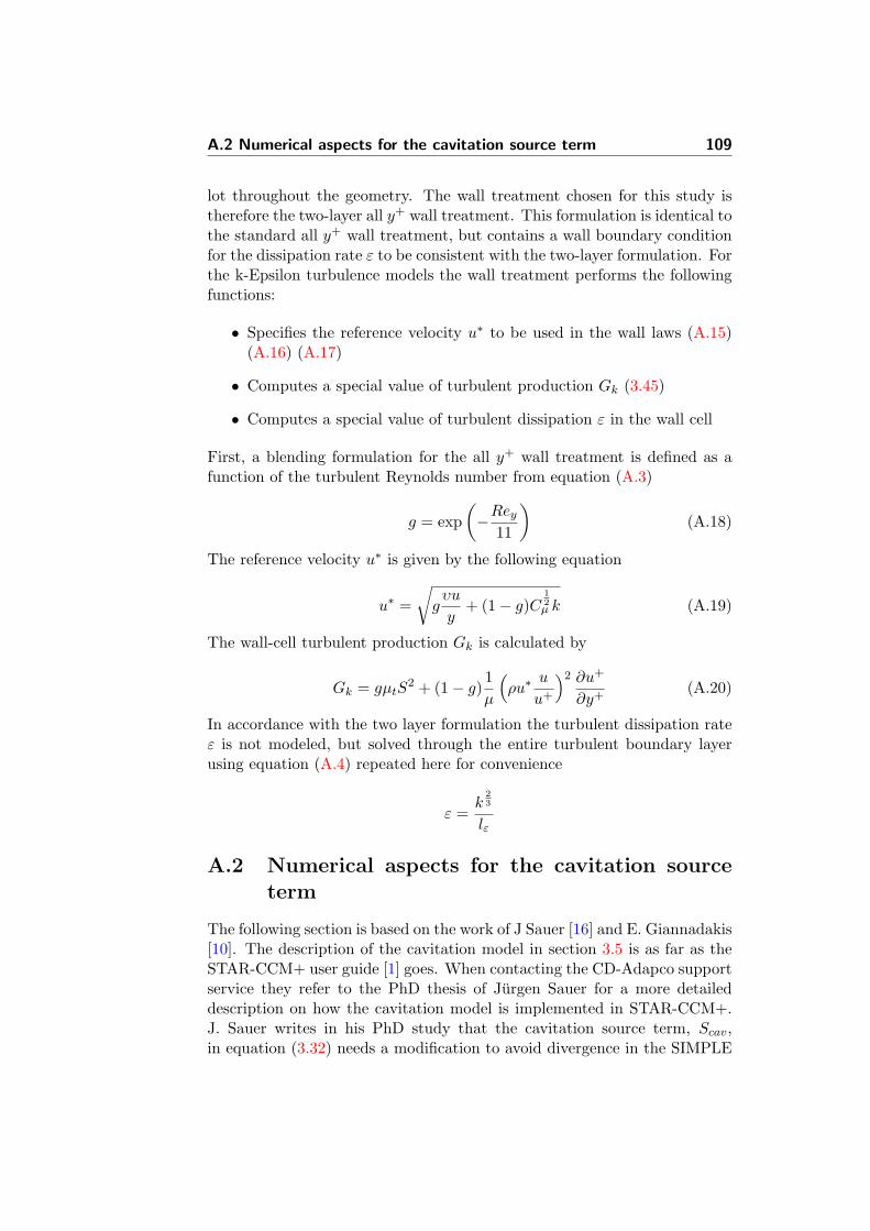
A.2 Numerical aspects for the cavitation source term 109

lot throughout the geometry. The wall treatment chosen for this study istherefore the two-layer all y+ wall treatment. This formulation is identical tothe standard all y+ wall treatment, but contains a wall boundary conditionfor the dissipation rate ε to be consistent with the two-layer formulation. Forthe k-Epsilon turbulence models the wall treatment performs the followingfunctions:

• Specifies the reference velocity u∗ to be used in the wall laws (A.15)(A.16) (A.17)

• Computes a special value of turbulent production Gk (3.45)

• Computes a special value of turbulent dissipation ε in the wall cell

First, a blending formulation for the all y+ wall treatment is defined as afunction of the turbulent Reynolds number from equation (A.3)

g = exp(−Rey

11

)(A.18)

The reference velocity u∗ is given by the following equation

u∗ =√gυu

y+ (1− g)C

12µ k (A.19)

The wall-cell turbulent production Gk is calculated by

Gk = gµtS2 + (1− g)

1µ

(ρu∗

u

u+

)2 ∂u+

∂y+(A.20)

In accordance with the two layer formulation the turbulent dissipation rateε is not modeled, but solved through the entire turbulent boundary layerusing equation (A.4) repeated here for convenience

ε =k

23

lε

A.2 Numerical aspects for the cavitation sourceterm

The following section is based on the work of J Sauer [16] and E. Giannadakis[10]. The description of the cavitation model in section 3.5 is as far as theSTAR-CCM+ user guide [1] goes. When contacting the CD-Adapco supportservice they refer to the PhD thesis of Jurgen Sauer for a more detaileddescription on how the cavitation model is implemented in STAR-CCM+.J. Sauer writes in his PhD study that the cavitation source term, Scav,in equation (3.32) needs a modification to avoid divergence in the SIMPLE

110 Appendix A

algorithm. The term Scav is an average value of the previous and the currenttime step since the bubble radius R is from the previous time step whilethe term dR

dt is from the current time step. This constitutes a mixture ofexplicit and pseudo implicit approach with respect to the time treatmentfor the source term[10] while the treatment for the pressure correction isonly pseudo implicitly. Treatment for the cavitation source term used bythe pressure correction equation is therefore necessary because the pressurecorrection estimations in the inner iterations of the SIMPLE algorithm leadsto divergence since it overcompensates pressure corrections e.g. where thepressure is below the vapor pressure. J. Sauer [16] proposed to include thepartial derivative of the cavitation source term with respect to the pressurecorrection of the current integration step to improve its implicitness andnumerical stability.

∂Smcav∂p

=n0

1 + n043πR

3· 4πR2 ∂

∂p

(dR

dt

)(A.21)

where

∂

∂p

(dR

dt

)=

∂∂p

(√23pv−p∞ρl

)= 1√

23pv−p∞ρl

· 23ρl

(−1) for growth

∂∂p

(√23p∞−pvρl

)= 1√

23p∞−pvρl

· 23ρl

(+1) for collapse(A.22)

or more general like

∂

∂p

(dR

dt

)=−23ρl

1√2

3ρl|pv − p∞|

(A.23)

including the above equations into the cavitation source term for the pressurecorrection the source term becomes

Smcav = Sm∗cav +∂Sm∗cav∂p

(pmp − pm∗p ) (A.24)

Where m is the iteration step for the SIMPLE algorithm.

DTU Mechanical Engineering

Section of Fluid Mechanics

Technical University of Denmark

Nils Koppels Allé, Bld. 403

DK- 2800 Kgs. Lyngby

Denmark

Phone (+45) 45 25 41 31

Fax (+45) 45 88 43 25

www.mek.dtu.dk

numerical simulation of the flow in fuel nozzles for...

Documents