Games Theory Notes From Strategies and Games: theory and practice by Prajit K. Dutta

Introduction

Block I: Strategic Form Games

Theme 1: Strategic Form

Theme 2: Dominance Solvability

Theme 3: Nash Equilibrium

Theme 4: Mixed Strategies

Theme 5: Symmetric Games

Theme 6: Zero-Sum Games

Block II: Extensive Form Games

Theme 7: Extensive Form

Theme 8: Backward Induction

Theme 9: Subgame Perfect Equilibrium

Theme 10: Finitely Repeated Games

Theme 11: Infinitely Repeated Games

Theme 12: Dynamic Games

Block III: Asymmetric Information Games

Theme 13: Games with Incomplete Information

Introducción

The foundations of game theory go back 150 years. The main development of the

subject is more recent, however, spanning approximately the last fifty years, making

game theory one of the youngest disciplines within economics and mathematics. The

earliest predecessors of game theory are economic analyses of imperfectly competitive

markets. The pioneering analyses were those of the economists Cournot and Edgeworth

(with subsequent advances due to Bertrand and Stackelberg). Cournot analyzed an

oligopoly problem, which now goes by the name of Cournot model and employed a

method of analysis which is a special case of the most widely used solution concept

found in modern game theory.

Modern game theory studies strategic situations. The focus of game theory is

interdependence, situations in which an entire group of people is affected by the choices

made by every individual within that group. A situation fails to be a game when your

decisions affect no one but yourself or there are so many people involved that it is no

feasible to keep track of what each one does. In interlinked situation, the interesting

questions include

What will each individual guess about the others' choices?

What action will each person take? (This question is especially intriguing

when the best action depends on what the others do.)

What is the outcome of these actions? Is it good for the group as a whole?

Does it make any difference if the group interacts more than once?

How do the answers change if each individual is unsure about the characteristics of

others in the group?

The content of game theory is a study of these and related questions. Moreover, we

can say that game theory is a formal way to analyze interaction among a group of

rational agents who behave strategically.

group In any game there is more than one decision-maker; each decision-

maker is referred to as a "player."

interaction What any one individual player does directly affects at least one

other player in the group.

strategic An individual player accounts for this interdependence in deciding

what action to take.

rational While accounting for this interdependence, each player chooses her

best action.

Although many situations can be formalized as a game, these notes introduce the

methodology of games, centering our attention in oligopolies and illustrating that

methodology with a variety of examples. However, when faced with a particular

strategic setting, it is necessary to incorporate its unique features in order to come up

with the right answer.

Every game is played by a set of rules which have to specify four things.

who: what group of players strategically interacts.

what: they are playing, what alternative actions or choices each player has

available

when: in what order each player gets to play

how much: what amount they stand to gain (or lose) from the choices made

in the game

The two principal representations of the rules of a game are called, respectively, the

normal form of a game (or strategic form) and the extensive form. Both forms are two

ways to represent a game. The normal form or strategic form is employed to study

games that are played simultaneously. Conversely, we will employ the extensive form

to study sequential game situations. The two representations are interchangeable; every

extensive form game can be written in strategic form and, likewise, every game in

strategic form can be represented in extensive form.

In games, every player knows the rules of a game and that fact is commonly known.

It is standard to assume common knowledge about the rules. That everybody has

knowledge about the rules means that if you asked any two players in the game a

question about who, what, when, or how much, they would give you the same answer.

This does not mean that all players are equally well informed or equally influential; it

simply means that they know the same rules.

Common knowledge of the rules goes even a few steps further: first, it says yes,

everybody knows that the rules are available to all. Second, it says that everybody

knows that everybody knows that the rules are widely available. And third, that

everybody knows that everybody knows that everybody knows, ad infinitum.

Example (prisoners' dilemma) Two prisoners, Calvin and Klein, are hauled in for a

suspected crime. The DA speaks to each prisoner separately, and tells them that she

more or less has the evidence to convict them but they could make her work a little

easier (and help themselves) if they confess to the crime.

She offers each of them the following deal: Confess to the crime, turn a witness for

the State, and implicate the other guy you will do no time. Of course, your confession

will be worth a lot less if the other guy confesses as well. In that case, you both go in for

five years. If you do not confess, however, be aware that we will nail you with the other

guy's confession, and then you will do fifteen years. In the event that I cannot get a

confession from either of you, I have enough evidence to put you both away for a year.

Notice that the entries in the above table are the prison terms. Thus, the entry that

corresponds to (Confess, Not Confess) the entry in the first row, second column is the

length of sentence to Calvin (0) and Klein (15), respectively, when Calvin confesses but

Calvin \ Klein Confess Not Confess

Confess 5, 5 0, 15

Not Confess 15, 0 1, 1

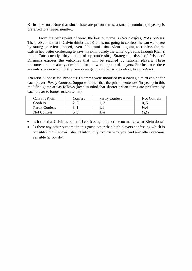
Klein does not. Note that since these are prison terms, a smaller number (of years) is

preferred to a bigger number.

From the pair's point of view, the best outcome is (Not Confess, Not Confess).

The problem is that if Calvin thinks that Klein is not going to confess, he can walk free

by ratting on Klein. Indeed, even if he thinks that Klein is going to confess the rat

Calvin had better confessing to save his skin. Surely the same logic runs through Klein's

mind. Consequently, they both end up confessing. Strategic analysis of Prisoners'

Dilemma exposes the outcomes that will be reached by rational players. These

outcomes are not always desirable for the whole group of players. For instance, there

are outcomes in which both players can gain, such as (Not Confess, Not Confess).

Exercise Suppose the Prisoners' Dilemma were modified by allowing a third choice for

each player, Partly Confess. Suppose further that the prison sentences (in years) in this

modified game are as follows (keep in mind that shorter prison terms are preferred by

each player to longer prison terms).

Is it true that Calvin is better off confessing to the crime no matter what Klein does?

Is there any other outcome in this game other than both players confessing which is

sensible? Your answer should informally explain why you find any other outcome

sensible (if you do).

Calvin \ Klein Confess Partly Confess Not Confess

Confess 2, 2 1, 3 0, 5

Partly Confess 3, 1 1,1 ¼,4

Not Confess 5, 0 4,¼ ½,½

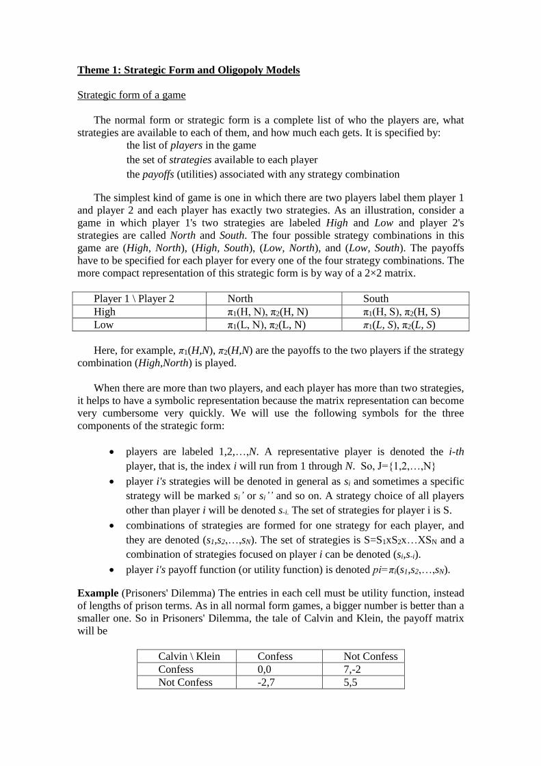
Theme 1: Strategic Form and Oligopoly Models

Strategic form of a game

The normal form or strategic form is a complete list of who the players are, what

strategies are available to each of them, and how much each gets. It is specified by:

the list of players in the game

the set of strategies available to each player

the payoffs (utilities) associated with any strategy combination

The simplest kind of game is one in which there are two players label them player 1

and player 2 and each player has exactly two strategies. As an illustration, consider a

game in which player 1's two strategies are labeled High and Low and player 2's

strategies are called North and South. The four possible strategy combinations in this

game are (High, North), (High, South), (Low, North), and (Low, South). The payoffs

have to be specified for each player for every one of the four strategy combinations. The

more compact representation of this strategic form is by way of a 2×2 matrix.

Player 1 \ Player 2 North South

High π1(H, N), π2(H, N) π1(H, S), π2(H, S)

Low π1(L, N), π2(L, N) π1(L, S), π2(L, S)

Here, for example, π1(H,N), π2(H,N) are the payoffs to the two players if the strategy

combination (High,North) is played.

When there are more than two players, and each player has more than two strategies,

it helps to have a symbolic representation because the matrix representation can become

very cumbersome very quickly. We will use the following symbols for the three

components of the strategic form:

players are labeled 1,2,…,N. A representative player is denoted the i-th

player, that is, the index i will run from 1 through N. So, J={1,2,…,N}

player i's strategies will be denoted in general as si and sometimes a specific

strategy will be marked si’ or si’’ and so on. A strategy choice of all players

other than player i will be denoted s-i. The set of strategies for player i is S.

combinations of strategies are formed for one strategy for each player, and

they are denoted (s1,s2,…,sN). The set of strategies is S=S1xS2x…XSN and a

combination of strategies focused on player i can be denoted (si,s-i).

player i's payoff function (or utility function) is denoted pi=πi(s1,s2,…,sN).

Example (Prisoners' Dilemma) The entries in each cell must be utility function, instead

of lengths of prison terms. As in all normal form games, a bigger number is better than a

smaller one. So in Prisoners' Dilemma, the tale of Calvin and Klein, the payoff matrix

will be

Calvin \ Klein Confess Not Confess

Confess 0,0 7,-2

Not Confess -2,7 5,5

Example (Battle of the Sexes) A husband and wife are trying to determine whether to

go to the opera or to a football game. The husband prefers the football game, the wife

prefers the opera but, at the same time, each of them would rather go with the spouse

than go alone.

Husband \ Wife football opera

football 3,1 0,0

opera 0,0 1,3

Example (Matching Pennies) Two players write down either heads or tails on a piece

of paper. If they have written down the same thing, player 2 gives player 1 a dollar. If

they have written down different things then player 1 pays player 2 instead.

Player 1 \ Player 2 heads tails

heads 1,-1 -1,1

tails -1,1 1,-1

Example (Hawk-Dove or Chicken) Two (young) players are engaged in a conflict

situation. For instance, they may be racing their cars towards each other on Main Street,

while being egged on by their many friends. If player 1 hangs tough and stays in the

center of the road while the other player concedes and chickens out by moving out of

the way, then all glory is his and the other player eats humble pie. If they both hang

tough they end up with broken bones, while if they both concede they have their bodies

but not their pride intact.

Player 1 \ Player 2 tough concede

tough -1,-1 10,0

concede 0, 10 5, 5

Example (War Game) In this war game, Colonel Blotto has two infantry units that he

can send to any pair of locations, while Colonel Tlobbo has one unit that he can send to

any one of four locations. A unit wins a location if it arrives uncontested, and a unit

fights to a standstill if an enemy unit also comes to the same location. A win counts as

one unit of utility; a stand still yields zero utility.

Tlobbo \ Blotto 1,2 1,3 1,4 2,3 2,4 3,4

1 0, 1 0, 1 0, 1 1, 2 1, 2 1, 2

2 0, 1 1, 2 1, 2 0, 1 0, 1 1, 2

3 1, 2 0, 1 1, 2 0, 1 1, 2 0, 1

4 1, 2 1, 2 0, 1 1, 2 0, 1 0,1

Example (Coordination Game) We can depict with matrices a strategic form game with

more than two players, such as in this coordination game where three players are trying

to coordinate to be together at a New York Knicks game at game time, 7:30P.M.

.

Player 3 plays 7:30

Player 1 \ Player 2 7:30 10:30

7:30 1, 1, 1 0, 0, 0

10:30 0, 0, 0 0, 0, 0

Player 3 plays 10:30

Player 1 \ Player 2 7:30 10:30

7:30 0, 0, 0 0, 0, 0

10:30 0, 0, 0 0, 0, 0

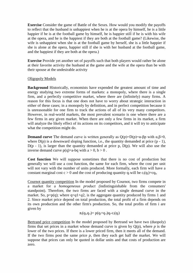
Exercise Consider the game of Battle of the Sexes. How would you modify the payoffs

to reflect that the husband is unhappiest when he is at the opera by himself, he is a little

happier if he is at the football game by himself, he is happier still if he is with his wife

at the opera, and he is the happiest if they are both at the football game? (Likewise, the

wife is unhappiest when she is at the football game by herself, she is a little happier if

she is alone at the opera, happier still if she is with her husband at the football game,

and the happiest if they are both at the opera.)

Exercise Provide yet another set of payoffs such that both players would rather be alone

at their favorite activity the husband at the game and the wife at the opera than be with

their spouse at the undesirable activity

Oligopoly Models

Background Historically, economists have expended the greatest amount of time and

energy studying two extreme forms of markets: a monopoly, where there is a single

firm, and a perfectly competitive market, where there are (infinitely) many firms. A

reason for this focus is that one does not have to worry about strategic interaction in

either of these cases; in a monopoly by definition, and in perfect competition because it

is unreasonable for one firm to track the actions of all of its very many competitors.

However, in real-world markets, the most prevalent scenario is one where there are a

few firms in any given market. When there are only a few firms in its market, a firm

will analyze the likely effect of its actions on its competitors, and it will try to anticipate

what the competition might do.

Demand curve The demand curve is written generally as Q(p)=D(p)=α-βp with α,β>0,

where D(p) is a downward sloping function, i.e., the quantity demanded at price (p - 1),

D(p - 1), is larger than the quantity demanded at price p, D(p). We will also use the

inverse demand curve p(q)=a-bq with a > 0, b > 0 .

Cost function We will suppose sometimes that there is no cost of production but

generally we will use a cost function, the same for each firm, where the cost per unit

will not vary with the number of units produced. More formally, each firm will have a

constant marginal cost c > 0 and the cost of producing quantity qi will be ci(qi)=cqi,

Cournot quantity competition In the model proposed by Cournot, two firms compete in

a market for a homogeneous product (indistinguishable from the consumers'

standpoint). Therefore, the two firms are faced with a single demand curve in the

market. So, p=p(q); where q=q1+q2, is the aggregate quantity produced by firms 1 and

2. Since market price depend on total production, the total profit of a firm depends on

its own production and the other firm's production. So, the total profits of firm i are

given by

πi(qi,q-i)= p(qi+q-i)qi-ci(qi)

Bertrand price competition In the model proposed by Bertrand we have two (duopoly)

firms that set prices in a market whose demand curve is given by Q(p), where p is the

lower of the two prices. If there is a lower priced firm, then it meets all of the demand.

If the two firms post the same price p, then they each get half the market. We will

suppose that prices can only be quoted in dollar units and that costs of production are

zero.

Exercise Write down the strategic form of Bertrand price competition assuming that

prices can be 0, 1, 2, 3, 4, 5, or 6 dollars; each firm cares only about its own profits and

the demand function is Q(p)=6-p

Battle for market share In this model we have two firms that set prices in a market

whose demand is fixed and, as in the Bertrand model, if there is a lower priced firm,

then it meets all of the demand and if the two firms post the same price p, then they

each get half the market.

Exercise Consider the market for bagels in the Morningside Heights neighborhood of

New York City where there are two bagel; Columbia Bagels (CB) and University Food

Market (UFM). Assume that prices are simultaneously chosen by University Food

Market and Columbia Bagels and that they can be 40, 45, or 50 cents. Assume that the

cost of production is 25 cents a bagel. Assume further that the market is of fixed size;

1000 bagels sell every day in this neighborhood and whichever store has the cheaper

price gets all of the business. If the prices are the same, then the market is shared

equally.

Write down the strategic form of this game, with payoffs being each store's profits.

Redo the same question such that the store with the cheaper price gets 75% of the

business. (Assume that everything else remains unchanged.)

Redo question yet again, presuming that Columbia Bagels has, inherently, the tastier

bagel and, therefore, when the prices are the same Columbia Bagels gets 75% of the

business. (Assume that everything else remains unchanged).

Theme 2: Dominance Solvability

Dominant Strategy Solution

Consider the Prisoners' Dilemma. The strategy confess has the property that it gives

Calvin a higher payoff than not confess if Klein does not confess (7 rather than 5). It

also gives him a higher payoff if Klein does confess (0 rather than -2). Hence, no matter

what Klein does, Calvin is always better off confessing. Similar logic applies for Klein.

In this game it is reasonable to predict that both players will end up confessing.

Definition A strategy, 𝑠𝑖′ , strongly dominates all other strategies of player i, if the payoff

to this strategy is strictly greater than the payoff to any other strategy, regardless of

which strategy is chosen by the other player(s).

πi(𝑠𝑖′ , 𝑠−𝑖) > πi(𝑠𝑖, 𝑠−𝑖) ∀𝑠𝑖 ≠ 𝑠𝑖

′𝑎𝑛𝑑 ∀𝑠−𝑖

A slightly weaker domination concept emerges if a strategy is found to be better

than every other strategy but not always strictly better:

Definition A strategy, 𝑠𝑖′ , (weakly) dominates another strategy, 𝑠𝑖

′′, if it does at least as

well as against every strategy of the other players, and against some it does strictly

better

πi(𝑠𝑖′ , 𝑠−𝑖) ≥ πi(𝑠𝑖′′, 𝑠−𝑖) ∀𝑠−𝑖

πi(𝑠𝑖′ , 𝑠−𝑖

#) > πi(𝑠𝑖𝑠−𝑖#) 𝑝𝑎𝑟𝑎 𝑐𝑖𝑒𝑟𝑡𝑜 𝑠−𝑖

#

In this case, we say that 𝑠−𝑖# is a dominated strategy. Moreover, when a strategy, 𝑠𝑖

′ , (weakly) dominates all other strategies we say it is a (weakly) dominant strategy. If a

strategy is not dominated by any other, it is called an undominated strategy. It is useful

to think of a dominated strategy as a "bad" strategy and an undominated strategy as a

"good" one. Of course, a dominant strategy is a special kind of undominated strategy,

namely one that itself dominates every other strategy. Put differently, it is the "best"

strategy.

Definition (dominant strategy solution) A combination of strategies is said to be a

dominant strategy solution if each player's strategy is a dominant strategy. When every

player has a dominant strategy, the game has a dominant strategy solution. The

problem with the dominant strategy solution concept is that in many games it does not

yield a solution. In particular, even if a single player is without a dominant strategy,

there will be no dominant strategy solution to a game. So, the solution concept fails to

give a prediction about play.

Exercise Consider the Bertrand price competition.

Show that the strategy of posting a price of $5 (weakly) dominates the strategy of

posting a price of $6. Does it strongly dominate as well?

Are there any other (weakly) dominated strategies for firm 1? Explain.

Is there a dominant strategy for firm 1? Explain.

Exercise Rework questions above, under the following alternative assumption: if the

two firms post the same price, then firm 1 sells the market demand (and firm 2 does not

sell any quantity).

Iterated Elimination of Dominated Strategies

Background Consider a game in which player has many strategies. Either of two things

have to be true. First, there may be a dominant strategy. All of the remaining strategies

are then dominated. Alternatively, there may not be a dominant strategy, in other words,

there may not be any best strategy. There has to be, however, at least one undominated

or good strategy (why?). The problem with the dominant strategy solution is that in

many games a player need not have a dominant or best strategy. What we will now

pursue is a more modest objective: instead of searching for the best strategy why not at

least eliminate any bad strategies (dominated)?

For the same reason that it is irrational for a player to play anything but a dominant

strategy (should there be any), it is also irrational to play a dominated strategy. The

reason is that by playing any strategy that dominates (this dominated strategy) she can

guarantee herself payoff which is at least as high, no matter what the other players do.

What is interesting is that this logic could then set in motion a chain reaction. In any

game once it is known that a player, player 1 for instance, will not play her bad

strategies, the other players might find that certain of their strategies are in fact

dominated. This is because othes players, player 2 for instance, no longer has to worry

about how his strategies would perform against player 1's dominated strategies. So,

some of player 2's strategies, which are only good against player 1's dominated

strategies, might in fact turn out to be bad strategies themselves. Hence, player 2 will

not play these strategies. This might lead to a third round of discovery of bad strategies

by some of the other players, and so on.

Indeed, in any game, if we are able to reach a unique strategy vector by following

this procedure, the strategy choice is said to be reached by iterated elimination of

dominated strategies (IEDS). So, we call the outcome the solution to IEDS and call the

game itself dominance solvable. The solution of this procedure can be multiple since

order of elimination matters. When strategies are dominated but not strongly dominated

the order of elimination matters, so we eliminate dominated strategies for all players

simultaneously in each round. Nevertheless, we cannot guarantee an outcome in any

case (see formal definition and further discussion in Dutta).

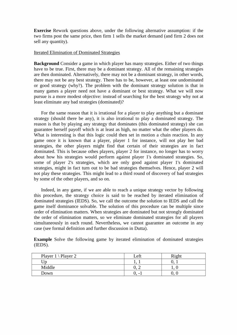
Example Solve the following game by iterated elimination of dominated strategies

(IEDS).

Player 1 \ Player 2 Left Right

Up 1, 1 0, 1

Middle 0, 2 1, 0

Down 0, -1 0, 0

For Player 1, the row player, neither of the first two strategies dominates each other,

but they both dominate Down. Hence, the row player should never play Down but

should rather play either Up or Middle. If it was known to player 2, the column player,

that 1 will never play Down, then, Right looks dominated to him. (Why?) Therefore, a

rational column player would never play Right. But then, the row player should not

worry about player 2 playing Right. Hence she would choose the very first of her

strategies, Up. So, (Up,Left)

Exercise (The Odd Couple) Felix and Oscar share an apartment. They have different

views on cleanliness and, hence, on whether or not they would be willing to put in the

hours of work necessary to clean. Suppose that it takes at least twelve hours of work

(per week) to keep the apartment clean, nine hours to make it livable, and anything less

than nine hours leaves the apartment filthy. Suppose that each person can devote three,

six, or nine hours to cleaning. Felix and Oscar agree that a livable apartment is worth 2

on the utility index. They disagree on the value of a clean apartment Felix thinks it is

worth 10 utility units, while Oscar thinks it is only worth 5. They also disagree on the

unpleasantness of a filthy apartment. Felix thinks it is worth -10 utility units, while

Oscar thinks it is only worth -5. Each person's payoff is the utility from the apartment

minus the number of hours worked. Write down the game strategic form and solve the

game by iterated elimination of dominated strategies (IEDS).

Bertrand price competition

Example (simple model) Suppose that either of two firms in a duopoly market can

charge any one of three prices high, medium, or low. Suppose further that whichever

firm charges the lower price gets the entire market. If the two firms charge the same

price, they share the market equally. These assumptions and any pair of prices translate

into profit levels for the two firms.

For example, firm 1 only makes a profit if its price is no higher than that of firm 2.

Suppose that the profits are given by the following payoff matrix.

Firm 1 \ Firm 2 high medium low

High 6, 6 0, 10 0, 8

medium 10, 0 5, 5 0, 8

Low 8, 0 8, 0 4, 4

Notice that the strategy high (price) is dominated by the strategy medium (and this is

true for both firms). Hence, we can eliminate high as an irrational strategy for both

firms (it either leads to no sales or a 50% share of a small market). Having eliminated

high we are left with the following payoff matrix.

We can now see that low dominates the medium price. Hence, the outcome to IEDS

is (low, low). Notice that medium is a useful strategy only if you believe that your

opponent is going to price high; hence, once you are convinced that he will never do so,

you have no reason to price medium either.

Firm 1 \ Firm 2 medium low

medium 5, 5 0, 8

low 8, 0 4, 4

In this example, there were two rounds of elimination. In the first, high price is

eliminated as dominated, and in the second round, medium price is then found to be

dominated and eliminated. The IEDS outcome is low price for each firm.

The analysis is easy to extend to the case where a firm can charge more than three

prices. The other two assumptions make sense if you imagine that this is a market with

no brand loyalty (because the products are identical) and all customers go to the vendor

who charges the lower price.

Exercise Consider Bertrand price competition:

Show that posting a price of 0 dollars and posting a price of 6 dollars are both

dominated strategies. What about the strategy of posting a price of $4? And $5?

Suppose for a moment that this market had only one firm. Show that the price at

which this monopoly firm maximizes profits is $3.

Based on your answer to the previous two questions, can you give a reason why in

any price competition model a duopoly firm would never want to price above the

monopoly price? (Hint: When can a duopoly firm that prices above the monopoly

price make positive profits? What would happen to those profits if the firm charged

a monopoly price instead?) *

Show that when we restrict attention to the prices 1, 2, and 3 dollars, the (monopoly)

price of 3 dollars is a dominated strategy.

Argue that the unique IEDS outcome is for both firms to price at 1 dollar.

There is a more general result about price competition. In any model of duopoly

price competition with zero costs the IEDS outcome is the lowest price at which each

firm makes a positive profit, that is, a price equal to a dollar.

Exercise Suppose, without loss of generality, that the monopoly price pm is 2 dollars or

greater and Q(p)=D(p), where D(p) is a downward sloping function

Show, by using similar logic to previous question, that charging a price above the monopoly

price pm is a dominated strategy.

Show that, as a consequence, charging price pm - 1 dominates the monopoly price.

Hint: Show that 1

2𝑝𝑚𝐷(𝑝𝑚) ≤ (𝑝𝑚 − 1)𝐷(𝑝𝑚 − 1). What can you assert about

1

2𝑝𝑚 versus 𝑝𝑚 − 1? What about D(pm) versus D( 𝑝𝑚 − 1)?

Generalize the above argument to show that if it is known that no price greater than

p will be charged by either firm, then p is dominated by the strategy of undercutting

to a price of p - 1, provided 2≤ p.

Conclude from the above arguments that the IEDS price must be, again, 1 dollar for

each firm.

Exercise Suppose, finally, that costs are not zero. Can you sketch an argument to show

that all of the previous results hold as long as the profits from undercutting to price p - 1

(and serving the entire market as a consequence) are higher than the profits from sharing

the market at price p?

Theme 3: Nash Equilibrium

Background Suppose that you have a strategy b that is dominated by another strategy,

say a. We have seen that it is never a good idea to play b because no matter what the

other player does, you can always do better with a. Now suppose you actually have

some idea about the other player's intentions. In that case, you would choose a provided

it does better than b given what the other player is going to do. You don't, in other

words, need to know that a performs better than b against all strategies of the other

player; you simply need to know that it performs better against the specific strategy of

your opponent.

Indeed, a is called a best response against the other player's known strategy if it does

better than any of your other strategies against this known strategy. Typically you will

not know exactly what the other player intends to do; at best you will have a guess

about his strategy choice. The same logic applies, however; what you really care about

is how a performs vis-à-vis b or any other strategy for that matter when played against

your guess about your opponent's strategy. It only pays to play a best response against

that strategy which you believe your opponent is about to play. Of course, your guess

might be wrong! And then you would be unhappy and you would want to change what

you did.

But suppose you and your opponent guessed correctly, and you each played best

responses to your guesses. In that case, you would have no reason to do anything else if

you had to do it all over again. In that case, you would be in a Nash equilibrium!

Definition A strategy, si’, is a best response to a strategy combination of the other

players, s-i, if

πi(𝑠𝑖′ , 𝑠−𝑖) ≥ πi(𝑠𝑖, 𝑠−𝑖) ∀𝑠𝑖

In other words, is a ''dominant strategy" in the very weak sense that it is a best

strategy to play provided the other players play the strategy combination s-i.

Definition The strategy vector (s1,s2,…,sN) is a Nash equilibrium if

πi(𝑠𝑖∗, 𝑠−𝑖

∗) ≥ πi(𝑠𝑖, 𝑠−𝑖∗) ∀𝑠𝑖 ∀𝑖

Each strategy si*, is a best response to the other players' strategy. Hence, si* is stable

and no player has an incentive to change his strategy from si* (see further discussion in

Dutta section 5.1)

Exercise Find Nash equilibriums in previous games.

Proposition Consider any game in which there is an outcome to IEDS. It must be the

case that this outcome is a Nash equilibrium. The reverse implication is not necessarily

true; there may be Nash equilibriums that are not the solution to IEDS.

Not all Nash equilibrium can be obtained as the outcome to IEDS. This point is easy

to see in any game in which there is a Nash equilibrium but the game is not dominance

solvable. Another situation where Nash does not imply IEDS can arise when there are

multiple Nash equilibriums; some of these Nash equilibriums would be eliminated by

iterated elimination of dominated strategies.

As regards the relation between dominant strategy solution and Nash equilibrium,

exactly the same result holds. First, note that every dominant strategy solution is an

IEDS outcome; if there is a dominant strategy every other strategy is immediately

eliminated. But we have just learned that every IEDS outcome is a Nash equilibrium. It

follows therefore that every dominant strategy solution is a Nash equilibrium. The

converse (again) need not hold.

Exercise Show that if there is a dominant strategy solution in which the strategies are

strongly dominant, then there cannot be any other Nash equilibrium

Bertrand price competition

Exercise Consider that the demand curve is given by D(p)=6-p, where p is the lower of

the two prices (and prices are quoted in dollar amounts). The lower-priced firm meets

all of the market's demand. If the two firms post the same price p, then each gets half

the market. Suppose that costs of production are zero.

Show that the best response to your rival posting a price of 6 dollars is to post the

monopoly price of 3 dollars. What is the best response against a rival's price of 5

dollars? And 4 dollars?

Can you show that the best response to 3 dollars is to price at 2 dollars instead?

Show that the Nash equilibrium of this price competition model is for each firm to

price at 1 dollar.

There is a more general result about price competition that can be established: In

any model of duopoly price competition with zero costs there is a single Nash

equilibrium; each firm charges the lowest price at which it makes a positive profit, that

is, one dollar.

Exercise Suppose that the demand curve is Q=D(p), where D(p) is a downward-sloping

function, denote the monopoly price pm and suppose pm≥2.

Show that if the rival firm charges a price above the monopoly price then the best

response is to charge the monopoly price.

Show further that if the rival firm charges a price p (> 1) at or below the monopoly

price, then the best response is to charge a price below p.

Hint: Can you show that charging a price p - 1, for example, is more profitable than

charging p or above?

Conclude from the preceding arguments that the unique Nash equilibrium price

must be, again, 1 dollar for each firm.

Exercise How would your answers to first exercise change if there were 3 firms in this

market? More generally, if there were N firms? Explain.

Exercise Suppose in the first exercise that firm 1 has unit costs of production; that is,

for every output level Q, its costs are Q dollars.

What is firm 1's best response to a price of 1 dollar (posted by firm 2)? Can you

show that firm 1 posting a price of 2 dollars and firm 2 posting a price of 1 dollar is

a Nash equilibrium?

Are the following prices a Nash equilibrium: firm 1 posts a price of 3 dollars, while

firm 2 prices at 1 dollar? What about 3 and 2, respectively? Can you demonstrate

that there cannot be a Nash equilibrium in which the firms post different prices

unless it happens to be 2 and 1 dollars, respectively (for firms 1 and 2)?

Argue that there cannot be a Nash equilibrium in which each firm posts a price of 2

dollars? Indeed show that there cannot be a Nash equilibrium in which the firms

post the same prices and these are above the minimum price of a dollar?

Show that there is a Nash equilibrium in which each firm posts a price of a dollar.

Cournot Duopoly

Background In the model proposed by Cournot, two firms compete in a market for a

homogeneous product and face a single demand curve in the market. We suppose that

the cost function is the same for each firm and that the cost per unit does not vary with

the number of units produced. Since market price depends on total production, the total

profit of a firm depends on its own production and the other firm's. So, the total profits

of firm i are given by

πi(Q1,Q2)=pQi-cQi=[a-b(Q1+Q2)-c]Qi

where Q1 and Q2 are firm 1 and 2 productions respectively

How much would each firm produce? To make that decision, each firm has to take

two steps. We will obtain an industry-wide or Nash-equilibrium when both firms

satisfactorily resolve corresponding issues.

Make a conjecture about the other firm's production. This step will give the firm

an idea about the likely market price; for instance, if it thinks the rival is going to

produce a lot, then the price will be low no matter how much it produces.

Determine the quantity to produce. To make this determination the firm has to

weigh the benefits from increasing production that is, that it will sell more units

against the costs of doing so that is, that these extra units will sell at a lower price

(and will need to be produced at a higher total cost).

Let us first analyze the two questions from the perspective of firm 1. If it was the

only firm in the market, firm 1's production decision would determine the market price.

It could then compute the profits from selling different quantity levels and pick the

quantity that maximizes profits. This is no longer true; the market price will depend on

both its own production Q1 and the other firm's production.

As a start, what firm 1 can do is ask what quantity it should produce in order to

maximize profits when firm 2 produces a given quantity.

𝑀𝑎𝑥𝑄1𝜋1(𝑄1 + 𝑄2) = 𝑀𝑎𝑥𝑄1[𝑎 − 𝑏(𝑄1 + 𝑄2) − 𝑐)𝑄1]

The quantity that maximizes profits can be determined by the first-order condition

and it is

𝑄1∗ =

𝑎 − 𝑐 − 𝑏𝑄2

2𝑏

What we have just computed is the best response of firm 1 to a quantity choice of

firm 2. Indeed, this formula gives us the best response of firm 1 for any quantity that it

conjectures firm 2 might produce. So we have shown that the best response function,

also called reaction function in the Cournot model, is

𝑅1(𝑄2) = {

𝑎 − 𝑐 − 𝑏𝑄2

2𝑏𝑄2 ≤

𝑎 − 𝑐

𝑏

0 𝑄2 ≥𝑎 − 𝑐

𝑏

By symmetric reasoning the best response function of firm 2 is given by

𝑅2(𝑄1) = {

𝑎 − 𝑐 − 𝑏𝑄1

2𝑏𝑄1 ≤

𝑎 − 𝑐

𝑏

0 𝑄1 ≥𝑎 − 𝑐

𝑏

There is a unique pair of quantities at which both best-response functions cross.

Hence this is a pair of quantities Q1* and Q2* for which

R2(Q1*)=Q2* and R2(Q1*)=Q2*

In other words, this pair is a Cournot Nash equilibrium of this game. In which we

can calculate the equilibrium quantities, price, and profits.

𝑄1∗ = 𝑄2

∗ =𝑎−𝑐

3𝑏 𝑝 =

𝑎+2𝑐

3 𝜋𝑖 =

(𝑎−𝑐)2

9𝑏

Cartel production

As a contrast let us compute the quantities that would be produced if the two firms

operate as a cartel, that is, if they coordinate their production decisions. If firms operate

as a cartel, it is reasonable to suppose that they set production targets in such a way as to

maximize their total profits.

Call the production "quotas" Q1 and Q2; these are selected so as to maximize the

total profits: We looked for a solution in which Q1=Q2. In general, it can be solved only

for Q=Q1+Q2.

𝑀𝑎𝑥𝑄𝜋𝑇(𝑄) = 𝑀𝑎𝑥𝑄[𝜋1(𝑄) + 𝜋2(𝑄)] = 𝑀𝑎𝑥𝑄[(𝑎 − 𝑏𝑄 − 𝑐)𝑄]

The difference between the cartel problem and the best response problem is that

here the two firms acknowledge explicitly that their profits are determined by their total

production. In the best response problem, however, each firm computes profits on the

basis of its own output alone (and assumes that the other firm would hold rigidly to

some quantity level). Again, the profit-maximizing aggregate quantity is characterized

by the first-order conditions. These two equations are easily seen to solve for the cartel

quantities, price, and profits

𝑄1∗∗ = 𝑄2

∗∗ =𝑎−𝑐

4𝑏 𝑝 =

𝑎+𝑐

2 𝜋𝑖 =

(𝑎−𝑐)2

8𝑏

Notice that if the firms operate as a cartel they produce a smaller quantity than in the

Nash equilibrium; the cartel output is 75 percent of the Cournot Nash equilibrium

output level. Both firms make lower profits in Nash equilibrium than if they operate as a

cartel (because in equilibrium they overproduce).

A natural question to ask is, Given that there are higher profits to be made in this

market, why don't the two firms increase profits (by cutting back production)? The

answer to this seeming puzzle, as with the Prisoners' Dilemma, is that what is good for

the group is not necessarily good for the individual. If the firms tried to produce as a

cartel, there would be incentives for each firm to cheat and increase its own profit at the

expense of the other firm.

If firm 2 produced the cartel quantity, 𝑎−𝑐

4𝑏, it follows from firm 1's reaction function

that its profit maximizing production level would be 3(𝑎−𝑐)

8𝑏; firm 1 would increase its

own profits by producing more than the cartel output level, 𝑎−𝑎

4𝑎. When Q1 increases

but Q2 does not, firm 2 is unambiguously worse off. After all, the market price goes

down, but firm 2 sells exactly the same amount.

The cartel weighs the profit loss of firm 2 against the profit gain of firm 1 and

chooses not to recommend a higher production quota than 𝑎−𝑎

4𝑎, Firm 1, in deciding

whether or not to cheat against this quota, simply notes that it can increase profits by

expanding output to its profit maximizing level.

Firm 1 ignores the effects of its cheating on firm 2's profit levels In the real world,

firms do not completely ignore the effect of their production on the profits of their

competitors. For instance, they worry about possible retaliation by competitors in the

future. These future considerations will be analyzed in Part III when we turn to dynamic

games.

Exercise The duopoly problem is different from the Prisoners' Dilemma in one

important respect, there is no dominant strategy. An easy way to see this point is to note

that the reaction function is a downward-Moping line; that is, the more the other firm

produces, the less a firm should produce in best response. What would the reaction

functions look like if there were a dominant strategy?

Stackelberg Model

Background In the Cournot analysis discussed up to this point, we presumed that the

two firms would pick quantities simultaneously. In his 1934 criticism of Cournot, the

German economist Heinrich von Stackelberg pointed out that the conclusions would be

quite different if the two firms chose quantities sequentially.

Suppose that firm 1 decides on its quantity choice before firm 2. How much should

each of the two profit maximizing firms produce? Note that firm 2's decision is made

when it already knows how much firm 1 is committed to producing. It follows from our

reaction function analysis that, if firm 1 is producing Q1, then firm 2 can do no better

than produce its best response quantity R2(Q1). Hence, in turn, firm 1 should choose the

value realizing that is going to be firm 2's subsequent production choice. In other words,

firm 1 should solve the following problem:

𝑀𝑎𝑥𝑄1𝜋1[𝑄1 + 𝑅2(𝑄1)] = 𝑀𝑎𝑥𝑄1[𝑎 − 𝑏(𝑄1 + 𝑅2(𝑄1)) − 𝑐)𝑄1]

Substituting R2(Q1) , we get

𝑀𝑎𝑥𝑄1

1

2[(𝑎 − 𝑏𝑄1 − 𝑐)𝑄1]

It follows from the first-order condition that the optimal choice is 𝑄1∗ =

𝑎−𝑐

2𝑏. We can

therefore conclude from firm 2's reaction function that 𝑄2∗ =

𝑎−𝑐

4𝑏

Exercise Check that firm 1's profits are higher in the Stackelberg solution than in the

Nash equilibrium but firm 2's are smaller.

The reason why firm 1 is able to make a higher profit is straightforward. By

committing to produce more than it would in the Nash equilibrium, firm I forces firm 2

to cut back on its own production. This commitment keeps the price relatively high

although lower than in the cartel solution but more importantly yields firm 1 two-thirds

of the market, as opposed to the market share of half that it gets in the Nash equilibrium.

Cournot model generalization

The Cournot model can be generalized in two directions. First, it is easy to

generalize the analysis to an oligopolistic market. If there are N firms in the market

producing identical products, the inverse demand function can be written, as P = a - bQ,

where Q is the aggregate quantity Q =Q1+ Q2+. . .+QN. If firm 1 conjectures the other

firms production then its profit-maximizing quantity is its best response.

In a Cournot-Nash equilibrium, it have to be Ri(Q*)=Qi* for all firm i. These

equations yield the following Nash equilibrium quantity 𝑄𝑖∗ =

𝑎−𝑐

(𝑁+1)𝑏. The total quantity

produced in the market is 𝑄∗ =𝑁(𝑎−𝑐)

(𝑁+1)𝑏, and the price at what it is sold is 𝑝 =

𝑎+𝑁𝑐

𝑁+1.

Note that as the number of firms becomes very large that is, as N approaches

infinity the price approaches the (marginal) cost of production c. In other words, an

oligopoly with many firms looks a lot like a perfectly competitive industry in which

competition drives price to marginal cost.

Exercise In the preceding analysis, we restricted ourselves to a Nash equilibrium in

which all firms produce the same quantities. Could there be any other equilibrium, that

is, equilibrium in which each firm might produce a different quantity? How would you

go about finding these asymmetric equilibrium?

Exercise Work out the cartel and Stackelberg solutions by following exactly the same

reasoning as in a duopoly.

A second generalization involves examining demand functions that are non-linear

and cost functions for which marginal cost rises with output. Under appropriate

restrictions on the demand and cost function, we can show that there is a Nash

equilibrium, that production is higher in this equilibrium than in a cartel solution, and

that the leading firm in a Stackelberg solution does better than in the Nash equilibrium.

The most usual restrictions include a decreasing and concave demand function and a

increasing and convex cost function.

Note To sum up

The Cournot model studies quantity competition among duopolistic firms facing

linear demand and with constant marginal cost.

It predicts play of a Nash equilibrium in quantities. In the Cournot Nash

equilibrium, each firm produces a greater quantity than it would produce as part

of a cartel. This result occurs because each firm ignores the adverse effect its

overproduction has on the other firm's profits.

There is an IEDS solution to the Cournot model, and it coincides with the

Cournot Nash equilibrium. If firm 1 can make an early commitment to a

production level, it can make more profits than in the Cournot Nash equilibrium

(Stackelberg solution).

Cournot version of the Bertrand price competition

Exercise we have a duopoly with inverse market demand p=6-q, each firm can only

choose one of the quantity levels 0, 1, 2, 3, . . . ,6 and costs of production are zero.

Write down the strategic form of this game.

What is the best response for firm 1 if it thinks that firm 2 will produce 4 units of

output? What if it thinks firm 2 will produce 2 units of output?

Show that the market price in Nash equilibrium is 2 dollars. Contrast your answer

with that under Bertrand competition.

What is the Stackelberg solution to this model? Detail any additional assumption

that you need to make to answer this question.

Differentiated goods duopoly model

Exercise Suppose that the two firms produce slightly different products and, as a

consequence, the first firm's price is more sensitive to its own product than that of firm

2. In particular, letting the outputs be denoted by q1 and q2, (qi = 0, 1, . . . .,7), suppose

the two demand curves are

𝑝1 = 7 −3

2𝑞1 −

1

2𝑞2 𝑝2 = 7 −

1

2𝑞1 −

3

2𝑞2

Write down the strategic form of this game. Argue that neither firm will produce an

output greater than 4 units.

What is firm 1's best response if it thinks that firm 2 is going to produce 2 units?

Find a Cournot Nash equilibrium for this duopoly model.

Exercise (continuous model) In this model any quantity can be produced and costs of

producing a unit is the same for both firms and is equal to c dollars.

The demand curves are

𝑝1 = 𝑎 − 𝑏𝑞1 − 𝑑𝑞2 𝑝2 = 𝑎 − 𝑑𝑞1 − 𝑏𝑞2 where b, d> 0 ; a > c.

Set up the best response problem for firm 1 and show that its best response function

is given by

𝑅1(𝑄2) = {

𝑎 − 𝑐 − 𝑑𝑄2

2𝑏𝑄2 ≤

𝑎 − 𝑐

𝑑

0 𝑄2 ≥𝑎 − 𝑐

𝑑

Compute the Cournot Nash equilibrium of this model.

Show that even in this model, the cartel produces less than what gets produced in

the Cournot Nash equilibrium.

Show that the ratio of cartel output to Nash equilibrium output is greater than the

corresponding ratio in the homogeneous-good case (3/4) if and only if b > d.

Exercise Suppose instead that the effect of the other firm's production is positively felt;

that is, d << 0 (assume also that b + d > 0).

Compute the Cournot Nash equilibrium of this model.

Compute the cartel quantities.

How does the Nash equilibrium output compare with the cartel output?

Theme 4: Mixed Strategies

Background Suppose that you are playing the game Battle of the Sexes. Seemingly,

you have only one of two choices to make go to the football game or the opera.

Actually, those are not the only choices you have. For instance, you can toss a coin. If it

comes up heads you can go to the football game, whereas if it comes up tails you can go

to the opera instead. Hence, you have at least three strategies to choose from: (a)

football, (b) opera, and (c) a coin toss, that is, a strategy with an equal likelihood of

going to football or opera. Notice that after the coin has been tossed, you will end up

doing one or the other football or opera. In that sense, the coin toss has not enlarged the

set of eventual actions available to you. However, it has clearly enlarged the set of

initial choices; strategy c is evidently distinct from a or b.

Before the coin lands, you are not sure and neither is your spouse whether you will

be at the game or at the opera house. Strategies a and b as well as every other strategy

that we have discussed so far are called pure strategies. A strategy such as c is called a

mixed strategy.. Indeed, strategy c is just one of many mixed strategies. For all distinct

likelihood of football versus opera, there is a corresponding mixed strategy. For

instance, there is a mixed strategy in which football is twice as likely an eventual choice

as the opera; this corresponds to a strategy in which the probability of playing the pure

strategy football is p while the probability of playing opera is 1-p.

Definition Suppose a player has M pure strategies, s1,s2,…sM. A mixed strategy for

this player is a probability distribution over his pure strategies; that is, it is a probability

vector (p1,p2,…,pM) with p1+p2+…+pM=1

Note Every pure strategy is also a mixed strategy. For instance, the pure strategy s1 is

equivalent to the mixed strategy in which p1=1 and pk= 0 for all other pure strategies.

Note Every mixed strategy's payoff is its expected payoff. Expected payoffs are

computed in two steps: Weight the payoff to each pure strategy by the probability with

which that strategy is played. Add up the weighted payoffs. It is obvious that a mixed

strategy's payoff depends on the strategies chosen by the other players.

Note If player 1 plays a mixed strategy p=(p1,p2,…,pM) and the other player play the

mixed strategy q=(q1,q2,…,qN). Then the expected payoff to player i is equal to

πi(p, q) = ∑ pkq

jπi(si

k, s−i

j)

k,j

Example In Matching Pennies calculate the expected payoff for player 1 of the mixed

strategy in which

player 1 plays h with probability p while player 2 plays t for sure.

player 1 plays h with probability p while player 2 plays h for sure

What are player 2's expected payoffs?

Example In Hawk-Dove (or Chicken) calculate the expected payoff for player 1 of the

mixed strategy in which

player 1 plays t with probability 1/3 while player 2 plays t for sure.

player 1 plays t with probability 1/3 while player 2 plays c for sure.

player 1 plays t with probability 1/3 while player 2 plays t with probability

1/2.

What are player 2's expected payoffs in this case

Example Consider this No-Name Game

Player 1 \ Player 2 L M1 M2 R

U 1,0 4,2 2,4 3,1

M 2,4 2,0 2,2 2,1

D 4,2 1,4 2,0 3,1

Suppose that player 1 plays U, M and D with probabilities .2, .3, and .5,

respectively, while player 2 plays only L and M2 with probabilities .4 and .6. Show

that player 1's expected payoffs equal 2.32. What about player 2's expected payoffs?

Calculate player 1's expected payoffs when player 1 plays U, M, D with

probabilities p1,p2, and p3, respectively, while player 2 plays L and M2 with

probabilities q and 1 - q.

Example (game of squash). In the middle of a rally you have to decide whether to

position your next shot in the front of the court or hit it to the back. Your opponent

likewise has to move in anticipation of your shot; he could start moving forward or

backward. Of course, if he does move forward, he is likely to finish off the rally if you

dropped your shot in front, but you are likely to win if you did in fact hit the hard shot

behind him. If he moves backward, converse reasoning applies. In the following table

are displayed the chances of winning the rally in the four possible cases:

Forward (F) Backward (B)

Front (f) 20,80 80,20

Back (b) 70,30 30,70

Suppose that you picked the strategy front (f). If your opponent correctly guessed

that you were going to make this choice alternatively, if in every rally you play f then he

will move forward (F) and he will win 80 percent of the rallies. By the same logic, if

you always picked b, or if this choice was correctly guessed, you would only win 30

percent of the rallies.

What happens, though, if you occasionally bluff half the time you go (and the other

half b)? If your opponent goes forward, you win 45 percent (the average of 20% and

70%) of the rallies, while if he goes backward, you win 55 percent of the rallies. In

other words, even though your opponent is correctly guessing (that you go f with

probability 1/2), you nevertheless win at least 45 percent of your rallies. This outcome

is in contrast with either of the pure strategies where your opponent could hold you

down to either 20 percent or 30 percent wins.

The intuition is also straightforward; if you are predictable, your opponent can pick

the move that will kill you (and win the game). If you are unpredictable that is, if you

use a mixed strategy he has no one move that is a sure winner. If he goes F, he gives up

on your shots to the back, and if he goes B he conversely loses when you hit to the

front. .

What percentage of the rallies do you expect to win if you are twice as likely to pick

f as you are to pick b and your opponent goes forward? What if he goes backward?

What is the minimum percentage that you will win from playing this mixed

strategy?

What about if you pick f in four out of ten rallies?

Definition Consider a mixed strategy given by a probability vector. The support of this

mixed strategy is given by all those pure strategies that have a positive probability of

getting played (in this strategy).

Note The expected payoff to a mixed strategy is simply an average of the component

pure-strategy payoffs in the support of this mixed strategy. If the payoffs to each of the

pure strategies in the support are not the same, then deleting all but the pure strategies

that have the maximum payoff must increase the average, that is, must increase the

expected payoff

Note A mixed strategy is a best response to a strategy if and only if each of the pure

strategies in its support is itself a best response to that strategy. Each of the remaining

strategies in the support yields the same payoff and any mixture of these strategies must

also be a best response.

Example In No-Name game in Dutta, take the column player's strategy to be R. The

implication simply says that a mixed strategy involving U and M is worse than U alone.

It further says that any mixed strategy that has U and D as its support is a best response.

Mixed Strategies and Dominance

Background A strategy does better than an alternative if it dominates the latter. It is

possible that a mixed strategy can dominate a pure strategy, even though no other pure

strategy is able to dominate it (see No-Name game in Dutta).

Note Adding mixed strategies changes absolutely nothing with regard to the dominant

strategy solution. If there is a pure strategy that dominates every other pure strategy,

then it must also dominate every other mixed strategy. (Why?) However, if there is no

dominant strategy in pure strategies, there cannot be one in mixed strategies either.

(Why?)

Note Mixed strategies do make a difference for the IEDS solution concept. A game that

has no IEDS solution when only pure strategies are considered can have an IEDS

solution in mixed strategies (see No-Name game in Dutta).

Note The worst-case payoff of a mixed strategy may be better than the worst-case

payoff of every pure strategy (see No-Name game in Dutta).

Mixed Strategies and Nash Equilibrium

Proposition In strategic form games there is always a Nash equilibrium (likely in mixed

strategies)

.

Example Analyze Nash equilibriums in the game of matching pennies and see that no

matter what pure strategy combination we examine, one of the players always has an

incentive to change his strategy. However, If player 1 mixes between heads and tails

with equal probabilities, then player 2 can do no better by switching from H to T (or

vice versa). Half the time she inevitably matches in either case. A similar logic applies

to player 1's choices if player 2 mixes between H and T with equal probabilities.

Example Analyze Nash equilibriums in the game of the Battle of the Sexes in which we

have already seen that there are two asymmetric pure strategy Nash equilibriums in this

game: (F, O) and (O, F) yielding payoffs of, respectively, (3,1) and (1, 3). Show that

there is also an asymmetric Nash equilibrium in which both players play the same

mixed strategy.

Exercise Show that if there is a pure strategy that dominates every other pure strategy,

then it must also dominate every other mixed strategy.

Exercise Show that if there is no dominant pure strategy, then there cannot be a

dominant mixed strategy either.

Exercise Find mixed-strategy Nash equilibriums in the game of Chicken

Exercise Are there mixed-strategy Nash equilibriums in the No-Name game?

Bertrand price competition

Exercise Consider Bertrand price competition

Show that if a mixed strategy q yields an expected payoff that is at least as high as

that from another mixed strategy p, against every pure strategy of the other player,

then it must also yield as high a payoff against every mixed strategy of the other

player. Conclude that we only need to check how each strategy does against the pure

strategy prices 0 through 6.

Show that any mixed strategy that places positive probability on a price of six

dollars that is, a mixed strategy p in which the probability p(6) > 0 is dominated.

Explain carefully the strategy that dominates p

Can you show that, as a consequence, any mixed strategy that places positive

probability on a price of five dollars that is, a mixed strategy p in which p(5)>0 is

dominated as well.

What is the outcome to IEDS in this game? Explain your answer carefully.

Theme 5: Symmetric Games

We are going to work with the game of Chicken but now we write the payoffs using

symbols rather than numbers, with d> b> 0 > a.

Player 1 \ Player 2 tough concede

tough a, a d,0

concede 0, d b, b

In other words, as a group, the players are better off if both concede rather than if

both act tough (b> a). However, if the other player is going to concede, then a player

has an incentive to be tough (d> b) and, conversely, against a tough opponent conceding

is better than fighting (0 > a).

There are exactly two pure-strategy equilibriums in this game; one of the players

concedes, while the other acts tough. Their payoffs are respectively 0 and d. There is

also a mixed-strategy equilibrium in this game, and let us now compute it.

Suppose that player 2plays t with probability p (and c with probability 1 -p). Then

the expected payoffs of player 1 from playing t are ap+d(1-p) and from playing c are

b(1-p). It follows that in a mixed-strategy best response of player 1, the two pure

strategies must give him the same expected payoffs. Hence, the probability p must

satisfy ap+d(1-p)=b(1-p) and hence 𝑝 =𝑏−𝑑

𝑎+𝑏−𝑑

If player 2 plays t with probability𝑝 =𝑏−𝑑

𝑎+𝑏−𝑑, then any mixed strategy is a best

response for player 1; in particular, the mixed strategy in which player 1 plays t with

exactly the same probability is a best response. Hence, we have there is a mixed-

strategy equilibrium in which the two players play identical strategies; each plays t with

probability 𝑝 =𝑏−𝑑

𝑎+𝑏−𝑑

The expected payoffs are the same for the two players and equal 𝑎𝑏

𝑎+𝑏−𝑑, a number

between the two pure-strategy payoffs of 0 and d.

Note In the numerical version, each plays t with probability 5/6 and c with probability

1/6, and the expected payoff is 5/6 for each player (while in the pure-strategy

equilibriums, the tough player gets 10 and the weakling gets 0).

Definition A game is symmetric if each player is identical to every other player, that is,

if each player has exactly the same strategy set and the payoff functions are identical

(πi(si′ , s−i

′′ ) does not depend on i). Roughly speaking, a symmetric game is one in which

each player is equal to every other player: each has the same opportunities, and the

same actions yield the same payoffs.

Note A two-player game is symmetric if and only if π1(s’,s’’)=π2(s’’,s’). As a

consequence, if they pick the same strategy they have the same payoffs,

π1(s’,s’)=π2(s’,s’).

Definition In a symmetric game a Nash equilibrium in which every player has the same

strategy is called a symmetric Nash equilibrium

Example Show that the mixed-strategy equilibrium in Chicken is a symmetric

equilibrium but the pure-strategy equilibriums are not.

Exercise Consider the payoff matrix of any symmetric 2 × 2 game, that is, any game

with two players and two pure strategies:

Player 1 \ Player 2 S1 S2

S1 a, a d, e

S2 e, d b, b

Write down parameter restrictions so that (S1,S1) is a symmetric Nash equilibrium.

Under what restrictions, can (S2,S2) be a symmetric Nash equilibrium? Are both

restrictions compatible; that is, can such a game have multiple pure-strategy symmetric

Nash equilibria?

Exercise Keep the parameters d and e fixed; that is, consider the same payoff matrix

with two free parameters a and b that can take on any values.

Suppose that a > e and d > b. What is the symmetric Nash equilibrium in this case?

Repeat the question when a > e but d > b. Be sure to check for more than one

symmetric Nash equilibrium in this case.

In this fashion, map out the entire set of symmetric equilibriums in this game.

Can you draw a figure, with the parameters a and b on the two axes, that shows the

symmetric equilibriums for each parameter combination?

Natural Monopoly

Background A natural monopoly is an industry in which technological or demand

conditions are such that it is "natural" that there be only one firm in the market. One

technological reason for a natural monopoly to arise is seen when the costs per unit of

production decline with the size of output. This phenomenon might occur if

There are increasing returns to scale in production. Increasing returns means

that twice as much output can be produced with less than twice as much input.

Consequently, total costs do not double when total output is doubled.

There are large unavoidable costs of doing business. For instance, there may be

a minimum size at which some inputs can be purchased; it may not be possible

to rent production space of size less than 10,000 square feet. Again, output can

be doubled without doubling input costs.The aircraft manufacturing industry is a

technological natural monopoly because of the large unavoidable costs

associated with manufacturing planes (and possibly, because of increasing

returns as well). Perhaps unsurprisingly, there is now a single domestic

manufacturer of large airplanes in the United States (Boeing having taken over

McDonnell Douglas).

Natural monopoly can also arise when demand is low (and consequently the only

way to make any money is to keep the price relatively high). Recall that duopoly

competition, whether Cournot or Bertrand, drives down the price.

The question that economists are most interested in is: how will a natural monopoly

become an actual monopoly? If we start off in an industry with two or more firms,

which firms will drop out? In many cases there are obvious candidates; firms with

higher costs will be the first ones to leave. If a firm has "deep pockets," then a rival will

throw in the towel earlier. If the products are differentiated, then the firm with greater

demand is more likely to remain. And so on. The question that remains is: how will a

natural monopoly become an actual monopoly when, to begin with, there are two (or

more) essentially identical firms in the market. An industry where this question is

immediately relevant is defense production. With the demise of the cold war and the

consequent decrease in military expenditures, there has been a substantial reduction in

demand. Will there be, for example, a single aircraft manufacturer to come out of

nowadays current lineup

Example Consider a duopoly that will last two more years, in which each firm is

currently suffering losses of c dollars per period. If one of the firms were to drop out,

then the remaining firm would make a monopoly profit of p dollars per period for the

remainder of the two years. Each firm can choose when to drop out: today (date 0), or a

year from now (date 1), or it can stay till the end (date 2). Furthermore, each firm only

cares about profits. These assumptions will all be relaxed in the more general analysis

of the next subsection. The payoff matrix is therefore

Firm 1 \ Firm 2 date 0 date 1 date 2

date 0 0, 0 0, π 0, 2π

date 1 π, 0 -c, -c -c, π-c

date 2 2π, 0 π-c, -c -2c, -2c

Let us first look for pure-strategy Nash equilibriums of this game. We assume that

π> c; that is, one monopoly period makes up for (the losses suffered in) a duopoly

period. If this were not the case, then the best response functions change but it does not

affect the equilibriums. (Why?)

Note that both firms have an identical best response function

b1 (date 0) = date 2, b1(date 1) =date 2, and b1(date 2) = date 0.

The game is in fact a version of Chicken. Think of date 0 as concede, date 2 as

tough, and the intermediate date 1 as medium. Now note that both conceding is better

than both playing tough (or medium). However, if the other player concedes then it is

better to play medium and better still to play tough while concede is the best option

against a medium or tough opponent.

Consequently, there are two asymmetric pure-strategy Nash equilibriums in this

game: one of the two firms drops out (i.e., concedes) at date 0 and the other then

remains in the market for the two years.

The problem is that there is no reason that firm I should think that firm 2, an

identical firm, is going to concede, especially since by conceding firm 2 would lose out

on 2p dollars worth of profits.

What of a symmetric mixed equilibrium? Let us turn now to that computation.

Suppose that firm 2 plays date 0 with probability p, date 1 with probability q, and date 2

with probability 1 - p - q. Firm 1's expected profits from its three pure strategies are

E1(date 0)=0

E1(date 1)=𝜋𝑝 − 𝑐(1 − 𝑝)

E1(date 2)=2𝜋𝑝 + (𝜋 − 𝑐)𝑞 − 2𝑐(1 − 𝑝 − 𝑞)

If there is to be a mixed-strategy best response for firm I that involves all three

dates; it must be the case that each strategy yields the same expected payoff.

CHECK (equal profits) Show that firm 1 is indifferent about its date of exit only if (a)

𝑝 =𝑐

𝜋+𝑐 and (b) q = 0

Hence, in particular, playing date 0 with probability 𝑝 =𝑐

𝜋+𝑐 and date 2 with

remaining probability 1 − 𝑝 − 𝑞 =𝜋

𝜋+𝑐 is a best response for firm 1 as well (q=0). This

then is the symmetric mixed-strategy Nash equilibrium.

Exercise Check, doing the necessary computations, that there are no other mixed-

strategy Nash equilibriums; for example, none involving only dates 0 and 1.

Exercise Consider a numerical example; suppose π = 10 and c = 2. In the symmetric

equilibrium, each firm drops out with probability 1/6 at date 0. If a firm does not drop

out at date 0, it remains till date 2. Calculate probability both firms exiting the market at

date 0 and probability they both stay the course, as well as, the remaining probability

one or the other leaves at date 0. Note that the first two outcomes both leaving and both

staying are collectively unprofitable; in the first case a market that would be profitable

for a monopoly is abandoned, while in the second case a market that is only profitable

for a monopoly remains a duopoly.

One interpretation of a mixed strategy is that it is based on events outside a firm's

control. For instance, a firm might believe that its rival will leave the market

immediately if the Fed's projection for GDP growth is less than 2 percent. If the firm

further believes that there is a likelihood p of such a projection, then it is as if it plays

against a mixed strategy with probability p on date 0. Alternatively, a firm may not

know some relevant characteristic about its rival, such as costs. If it believes that high-

cost rivals will exit at date 0 but not low-cost ones and that the likelihood of high costs

is p, then again it is as if it faces a mixed strategy with probability p on date 0.

War of Attrition

The previous conclusion that a firm will only consider the extreme options of

leaving immediately and leaving at the end continues to hold in a more general version

of Chicken called the War of Attrition. Suppose that instead of three dates, there are N +

1 dates; a generic date will be denoted t. As before, a monopolist makes profits of π

dollars per period, while a duopolist suffers losses of c dollars per period. The payoff

matrix is

The War of Attrition retains the essential features of Chicken; both players

conceding immediately is better collectively than both conceding simultaneously but

later. If the rival concedes at date t, and a firm is still in the market at that date, then it is

best to go all the way to date N.

Exercise Let us first look at the pure-strategy Nash equilibriums. Start with the best

response function of firm 1 and suppose that firm 2 is going to drop out at date t.

Show that the best response to date t must be either date 0 or date N. The former

strategy yields a payoff of 0, while the latter yields a payoff of (N - t)p-tc.

Calculate the best response function of firm 1

Show that even in this more general game there are exactly the same two pure-

strategy equilibriums; one of the two firms drops out at date 0, but the other stays

till date N.

Exercise What of symmetric mixed-strategy equilibriums? In principle, a firm can exit

the market at any date between 0 and N with positive probability. We will show,

however, that a firm will never choose an intermediate date at which to exit; either it

will leave at date 0, or it will stay till date N. This conclusion will seem intuitive given

what we just saw about the best response functions. We have to be a little careful,

however; the rival can now play a mixed strategy, and the best response function that

we have so far analyzed was only computed against a pure strategy of the rival.

Proof that every pure strategy other than date 0 and date N is dominated by

some mixed strategy that has date 0 and date N in its support

Since the mixed strategy dominates the pure strategy, the latter will never be used in

a best response even if the rival firm plays a mixed strategy. (Why?) Hence, in order to

compute the mixed-strategy equilibrium we can concentrate on date 0 and date N alone.

Put differently, qualitatively the same symmetric mixed strategy equilibrium that we

computed in the previous subsection is the symmetric mixed-strategy equilibrium of this

general model as well

We have assumed so far that a firm makes a once-for-all decision about its exit date.

In practice, if a firm finds itself as a monopoly, it should abandon any earlier

commitment to drop out by date t and instead should stay till date N. We can generalize

the analysis to incorporate this possibility. In this general analysis it is possible that a

firm might stay till intermediate dates such as 1,2,...,N-1.

Natural Monopoly General Analysis

Exercise Consider the following numerical version of the natural monopoly problem

Firm 1 \ Firm 2 date 0 date 1 date 2

date 0 0, 0 0, 15 0, 30

date 1 15,0 -5, -5 -5,10

date 2 30, 0 10, -c -10, -10

Compute the symmetric equilibrium.

What is the expected payoff of each firm in equilibrium?

What is the probability that exactly one of the firms will drop out of the market at

date 0 in the symmetric equilibrium?

Exercise Redo parts a and b of previous exercise but with an increase in the costs of

staying from 5 dollars to 10 dollars (see payoff matrix) How does this cost increase

affect the probability that exactly one firm exists on the market at date 0?

Firm 1 \ Firm 2 date 0 date 1 date 2

date 0 0, 0 0, 15 0, 30

date 1 15,0 -10, -10 -10,5

date 2 30, 0 5,-10 -20, -20

Exercise Consider the general version of the natural monopoly problem

Firm 1 \ Firm 2 date 0 date 1 date 2

date 0 0, 0 0, π 0, 2π

date 1 π, 0 -c, -c -c, π-c

date 2 2π, 0 π-c, -c -2c, -2c

In the symmetric mixed-strategy equilibrium of this game, can you tell whether

dropping out at date 0 is more likely if costs c increase? And if profits π decrease?

Explain your answer.

How is the probability that exactly one firm drops out at date 0 affected if c

increases? And if π decrease? What about the probability that at least one firm drops

out?

Does an increase in c make a monopoly more likely? And a decrease in π?

Is there a sense in which an increase in costs and a decrease in profits have exactly the same

effect on market outcomes, that is, exactly the same effect on the symmetric equilibriums of

the game?

Exercise This question will explore the interpretation that date t really is the following

strategy: ''If my opponent has not dropped out by date t - 1, then I will drop out at t;

otherwise I will continue till the end."

Argue that the consequent payoff matrix when there are three exit dates becomes

Firm 1 \ Firm 2 date 0 date 1 date 2

date 0 0, 0 0, 2 π 0, 2 π

date 1 2 π, 0 -c, -c -c, π -c

date 2 2 π, 0 π -c, -c -2c, -2c

What are the pure-strategy Nash equilibria of the game?

Compute the symmetric mixed-strategy equilibrium of this game.

How do the expected payoffs in this symmetric equilibrium compare with the one

that follows from basic general case?

What about the probability that at least one of the firms drops out at date 0?

Theme 6: Zero-sum games

Background These games are more important, perhaps, because of the historical role

they have played in the development of the subject; that, by itself, is a reason to discuss

them. A second reason is that several concepts that were first introduced for zero-sum

games have turned out to be very useful for non-zero-sum games as well. We will try to

point out which of the results and concepts of zero-sum game theory are valid even

outside its confines.

A zero-sum game is one in which the payoffs of the two players always add up to

zero, no matter what strategy vector is played In a (two-player) zero-sum game the

payoffs of player 2 are just the negative of the payoffs of player 1. Consequently, the

incentives of the two players are diametrically opposed one player wins if and only if

the other player loses. Most games that are actual sporting contests are zero-sum games

size and so it is Matching Pennies. The battle for market share by two firms in a market

of fixed is not a zero-sum game but the total profit of the two firms is constant, since the

market is of fixed size. We will see while that such a situation can be effectively

reduced to a zero-sum game.

Many economic applications are, on the other hand, not zero-sum games, for

instance; the Cournot duopoly and the natural monopoly problem. In the Cournot

problem, collective profits are highest if total production is at monopoly level, but these

profits are a lot lower if each firm overproduces. In the natural monopoly problem, if

both firms remain in the market, they lose money, but it is profitable for only one of

them to remain. Zero-sum games are studied only in the case where there are two

players. Hence, we will say "zero-sum game" rather than "two-player zero-sum game"

whenever we refer to this category of games. To avoid clutter we will refer to zero-sum

games and constant-sum games as zero-sum games.

Definition A zero-sum game is one in which for all strategies s1 and s2 the payoffs of

the two players always add up to zero, π1(s1,s2)+π2(s1, s2)=0.

A constant-sum game is one in which the payoffs of the two players always add up

to a constant, say b, π1(s1,s2)+π2(s1, s2)=b

Example In the game of squash the two payoffs always add to 100 if we subtract this

constant from every payoff of one of the player the game becomes a zero-sum game.

The players would play this zero-sum transformation exactly the same way that they

would play the original constant-sum game. Furthermore, we will only write player 1's

payoff, since player 2's payoff is simply the negative of player 1's. Accordingly we will

drop the player subscript in the payoff function. For variety's sake we will changed the

payoffs just a little bit. So, the squash game's payoffs will be written:

Forward (F) Backward (B)

Front (f) 20 70

Back (b) 90 30

Playing Safe: Maxmin

In a zero-sum game player 2 does well if and only if player I does badly. For any

strategy s1, there is a strategy b(s1) that player 2 can select that makes his payoff the

highest possible and simultaneously makes player 1's the lowest. The strategy b(s1) is

such as

𝜋(𝑠1, 𝑏(𝑠1)) = min𝑠2

𝜋(𝑠1, 𝑠2)

In the conservative approach, player I presumes that no matter which strategy she

plays, player 2 will correctly anticipate it and play the worst-case or payoff-minimizing

strategy b(s1). Hence, in order to play it safe, player I should play that strategy s1 whose

worst-case payoff is better than the worst-case payoff to every other strategy It is

important that, in choosing her best worst payoff, player I consider mixed strategies as

well. (This is exactly the same concept that was called the Stackelberg solution when

we discussed the Cournot model).

Definition The guaranteed payoff (or best worst-case payoff) is called the maxmin

payoff and denoted m1

m1 = maxp

min𝑠2

𝜋(𝑝, 𝑠2)

where π(p, s2) is player 1's expected payoff when she plays a mixed strategy p and

player 2 plays a pure strategy s2

Note In the definition of a maxmin payoff, we only consider pure strategies for player 2

while considering mixed strategies for player 1. The reason is that player 2 gets no

higher payoff from playing any mixed strategies q; that is,

min𝑠2

𝜋(𝑝, 𝑠2) = min𝑞

𝜋(𝑝, 𝑞)

Definition The strategy that guarantees player 1 her maxmin payoff is called her

security strategy. So, a strategy p* is a security strategy for player 1 if

𝜋(𝑝 ∗, 𝑏(𝑝 ∗)) = m1

Note Since the strategy b(p) minimizes player 1's payoff, it is a best-response for player

2 against p (and hence the notation). Consequently, the safe approach is one in which a

player expects her opponent to play a best-response strategy and wants to guard against

any consequent adverse outcomes.

Note The safe approach gives player 1 a unilateral way to play the game. She knows

that she can do no worse than m1 if she plays her security strategy p*. If her opponent

in fact does not play a best response, then her payoffs can only be higher. This is unlike

best-response behavior, which requires player 1 to think through the question: what is it

that I am best responding to? Of course such unilateralism may come at a price; safe

play may not be as profitable as best response play.

Example Compute the maxmin payoff in Matching Pennies

To begin with, let us compute the maxmin payoff if player I only uses pure

strategies. Regardless of whether player I plays H or T, her payoffs are at a minimum if

player 2 mismatches; in each case player 1's payoff is -1, and so her pure-strategy

maxmin payoff is -1.

However, suppose that player 1 does use mixed strategies. Let p denote the

probability with which she plays H. If player 2 plays H for sure, player 1's expected

payoffs are 2p-1, while if player 2 plays T for sure, then player 1's expected payoffs are

1 - 2p. (Why?)

The two sets of expected payoffs are graphed in Dutta’s Figure 10.1. The minimum

payoff for any player is the smaller of the two payoffs; that is, it is the lower envelope

of the two expected payoff lines in the figure. It is clear that the highest minimum

payoff is realized where the two expected payoff lines intersect, at p*=1/2. Furthermore,

the maxmin payoff is 0. Note that this mixed-strategy maxmin payoff is higher than the

pure-strategy maxmin payoff computed earlier. This is another instance where a mixed

strategy guarantees a player a higher worst-case payoff than the pure strategies.

Exercise Compute the maxmin payoff in Squash Game

Note Player 2's maxmin payoff is denoted m2 and is defined as

m2 = maxs1

min𝑞

− 𝜋(𝑠1, 𝑞)

Notice that we have used the fact that player 2's payoffs are opposite to player 1's

payoffs. Let q* denote the security strategy of player 2; m2 is the highest payoff that

player 2 can guarantee himself (and he can do that by playing q*).

Playing Sound: Minmax

Background In the previous section we reached the following conclusion: player 1's

payoffs must be at least as high as her maxmin payoffs, m1, and she can guarantee these

payoffs by playing safely, that is, by playing her security strategy p*. In this section we

will see that there is an alternative (sound!) way for player1 to play the game.

Instead of playing to guard against worst-case outcomes, player 1 could play "more

aggressively" by playing best responses against player 2's strategies. One could think of

this as the more optimistic approach; try to predict the opponent's play and do the best

against it. The associated concept is called the minmax payoff; it is the worst of the best

(response) payoffs for player 1 (and is denoted M1)

M1 = minq

max𝑠1

𝜋(𝑠1, 𝑞)

where, again, π(s1,q) is the expected payoff to player 1 when she plays the pure strategy

s1 and her opponent plays the mixed strategy q.

Note In the minmax definition we restrict attention to pure strategies for player 1 while

considering mixed strategies for player 2 because player 1 can do no better by using

mixed strategies (Why?)

Example Compute the minmax payoff in Matching Pennies

The pure-strategy minmax payoff of player 1 is 1. If, instead, player 2 plays a mixed

strategy, say, plays H with probability q, then player 1's payoffs from playing H and T

are, respectively, 2q- 1 and 1 - 2q. As before, these expected payoffs are graphed in

Dutta´s Figure 10.3. The maximum of these expected payoffs is the upper envelope of

these two lines. The minmax payoff is then the lowest value of these maximum

expected payoffs; that is, the mixed-strategy minmax is 0. Note that these payoffs are

realized when q*=1/2; that is, they are realized when player 2 plays his security

strategy. Player 1 realizes her maxmin payoff (0) by playing her security strategy; she

gets her minmax payoff (0) when her opponent, player 2, plays his security strategy.

Exercise Compute the minmax payoff in Squash Game

The examples illustrate two very general results. The first is that by playing the best-

response approach, a player can do no worse than by playing safely. The second is that

one person's safe approach is another player's best-response approach.

Proposition (Minmax is better than Maxmin). The minmax payoff of player 1 is at least

as high as her maxmin payoff, that is, m1≤M1 (Conversely, player 2's minmax payoff is

at least as much as his maxmin payoff).

Note The result that a player's minmax payoff is at least as high as his maxmin payoff

holds in all games; whether they be zero-sum or nonzero-sum and whether they be two-

player or many-player games (this statement is true regardless of whether we consider

pure or mixed strategies).

Proposition (One's Minmax is the other's Maxmin). The minmax payoff of player 1 is

precisely (the negative of) the maxmin payoff of player 2, that is, m1=-M2 (Conversely,

the minmax payoff of player 2 is the negative of the maxmin of player 1.)

Note To sum up

Safe Strategy Player 1 can guarantee herself a payoff of at least m1 by

playing her security strategy p*; she gets exactly m1 when her opponent plays

his best response to p*.

Sound Strategy Player 1 cannot get payoffs any higher than her minmax

payoff M1 if player 2, in turn, plays his security strategy q*. She gets exactly

M1 by playing a best response to q*

Playing Nash: Playing Both Safe and Sound

What if both players played best responses; that is, what if we have a Nash

equilibrium? Well, somewhat remarkably, that situation turns out to be the same thing

as both players playing safe! We will see that any pair of strategies that constitute a

Nash equilibrium of a zero-sum game also constitutes a pair of security strategies for

the two players and vice versa; that is, the security strategies form a Nash equilibrium,

provided the maxmin and minmax payoffs are equal to each other.

Proposition (characterization of Nash equilibriums in zero-sum games) A pair of mixed

strategies is a Nash Equilibrium of a zero-sum game if for all pure strategies s1 and s2

𝜋(𝑠1, 𝑞 ∗) ≤ 𝜋(𝑝 ∗, 𝑞 ∗) ≤ 𝜋(𝑝 ∗, 𝑠2)

Note The first inequality says that p* is a best response against q*. On the other hand,

the second inequality says that player 1's payoffs are minimized, among all possible

strategies of player 2, by the choice of q*. That statement, of course, is the same thing

as saying that q* is a best response for player 2 against p*.

Proposition (playing Safe and Sound). Let (p*,q*) constitute a Nash equilibrium of a

zero-sum game, then, p* and q* are security strategies and the maxmin and minmax

payoffs are equal to each other and to π(p*,q*). Conversely, suppose that the minmax

and maxmin payoffs are equal, then, the security strategies constitute a Nash

equilibrium of the game.

Battle for market share

Exercise Consider the following two-firm pricing game in which two firms are

competing in a market of fixed size. They can choose either of two prices high and low

and care only about their market share:

Columbia / H&H High Low

High 60, 40 30, 70

Low 80,20 50, 50

Turn this into a zero-sum game.

Compute the security strategy for each firm as well as the maxmin payoff.

Exercise Based on your answer to the previous question, what can you conclude about

the security strategy and the maxmin payoff if each of the two players has a dominant

strategy in the game? What if only one of them has a dominant strategy?. What can you

conclude about the minmax payoff in either of the two preceding situations? (Use game

examples if you need to in order to make your point.)

Exercise Consider a variant of the two-firm pricing game in which firms can choose

either of two prices high and low (in Dutta levels of advertising expenditures) and care

only about long-run market share

Columbia / H&H High Low

High 0, 100 70, 30

Low 40,60 30, 70

Turn this into a zero-sum game.

Compute the maxmin payoffs and the security strategy for Columbia Bagels. Do this

computation first for pure strategies alone and then for mixed strategies.

What are the maxmin payoffs for H&H Bagels?

Exercise Consider the following variant in which H&H Bagels has a third strategy of

pricing. The payoffs for Columbia Bagels in this case are

Columbia / H&H High Modest Low

High 0 10 70

Low 40 36 30

Compute the pure-strategy maxmin payoffs and the security strategy for Columbia

Bagels. Then repeat the exercise for mixed strategies

What are the maxmin payoffs for H&H Bagels?

Exercise Consider the following variant in which both firms has the third strategy of

pricing modest. The payoff matrix is as follows:

Columbia / H&H High Modest Low

High 0 10 70

Modest 15 50 60

Low 40 36 30

Compute the pure-strategy maxmin payoff and minmax payoff for Columbia

Bagels.

Now compute the (regular) maxmin and minmax payoffs.

What are the Nash equilibriums of this game?

Theme 7: Extensive Form

Definition (basic concepts and terminology of the extensive form). The extensive form

is a pictorial representation of the rules. This form is pictured by way of a game tree

that starts from a unique node called the root. Out of the root come several branches

and at the end of each branch is a decision node. In turn, branches emanate from each of

these decision nodes and end in yet another set of nodes. A decision node is a point in

the game where one player and only one player has to make a decision. Each branch of

the tree emanating from that node corresponds to one of his choices. If a node has no

branches emerging from it then it is called a terminal node (and the game ends at that

point). An information set is made up of nodes that are indistinguishable from the

decision maker's standpoint and represents simultaneous moves by means of an oval

that encircles those nodes. In the extensive form of a game a player is any individual

who has a decision node in the game tree. The branches that come out of a decision

node represent what are the different choices available at that point. A node is reached

only when the previous choices have been made. The key idea to represent

simultaneous moves within the extensive form is that a player will act in the same way

in either of two circumstances; first, if he literally chooses at the same time as his

opponent and second, if he actually chooses after his opponent but is unaware of his

opponent's choice.

Note A strategy for a player specifies what to do at every information set at which the

player has to make a choice. More precisely, since a player cannot distinguish between

the nodes within any one information set, a strategy specifies what to do at each set. A

player's strategy is a complete, conditional plan of action. It is conditional in that it tells

a player which branch to follow out of a decision node if the game arrives at that node.

It is complete in that it tells him what to choose at every relevant decision node. In any

game, a collection of strategies, one for each player, will determine which branch of the

game tree will actually get played out.

.

Exercise (Get the Ticket or Theater Game) Two players are on their way to see a

Broadway musical that is in so great demand that there is exactly one ticket left and

whoever arrives first will get that ticket (if they happen to be at the same time there is a

50 percent chance that each player will get the ticket). The theater-goers have to decide

which form of transportation b(bus), c(cab), or s(subway) they should take to the

Theater. A cab is faster than the subway, which, in turn, is faster than the bus. Payoffs

depend on ticket availability as well as the mode of transportation.

First player leaving home earlier Both players leaving at the same time

Exercise What form has player’s strategies? How many strategies are there?

Distinguish between the first player leaving home a little earlier than player 2 or both

leaving at the same time.

Note In order for a tree to represent a game, the nodes and the branches need to satisfy

three consistency requirements:

1. Single Starting Point. It is important to know where a game starts, and so there

must be one, and only one, starting point.

2. No Cycles. It is important that we not hit an impasse while playing the game; it

must not be possible for the branches of a tree to double back and create a cycle.

3. One Way to Proceed. It is important that there be no ambiguity about how a

game proceeds, and so there must not be two or more branches leading to a node

Definition The predecessors of a node A are those nodes from which you can go

through a sequence of branches to A.

Note To guarantee the three consistency requirements, the following restrictions are

imposed on predecessor nodes:

1. A node cannot be a predecessor of itself

2. A predecessor's predecessor is also a predecessor: if a node B is a predecessor of

A and a node C is a predecessor of B, then C is a predecessor of A as well.

3. Predecessors can be ranked: if B and C are both predecessors of A, it must be

the case that either B is a predecessor of C or vice versa.

4. There must be a common predecessor: Consider any two nodes, A and B, neither

of which precedes the other. Then there must be a node C that is a predecessor

of both A and B.

Note A mixed strategy is defined in exactly the same way as in the strategic form; it is

simply a probability distribution over the pure strategies.

Note We can also build uncertainty that is inherent to the game (as opposed to

uncertainty that the players introduce via mixed strategies) into the extensive form. One

way to model that possibility is to allow for a third kind of node, called a chance node;

this is a node whose branches represent several random possibilities.

Definition A game of perfect information is a game whose extensive form has the

property that there is exactly one node in every information set. So, there is no

information set with multiple nodes.

Note A game of perfect information cannot have any simultaneous moves.

Entry games

Example (Entry game I) Coke is debating whether or not to enter a new Market (FSU)

where the market is dominated by Pepsi. Coke's decision is guided by the potential

profitability of this new market, and that depends principally on how Pepsi is going to

react to Coke coming into its market. If Pepsi mounts a big advertising campaign,

spends a lot of money upgrading facilities, ties up retailers with exclusive contracts in

other words, acts ''tough" then Coke will lose money. On the other hand, if Pepsi were

not to mount such a tough counterattack which is costly Coke would make money. We

use for Coke's alternatives E for enter and O for stay out, whereas T for tough and A for

accommodate refer to Pepsi's two choices on how to counter Coke's entry.

Example (Entry game II) Let us consider the following variant. Suppose that after

Pepsi's decision, Coke has a further decision to make; it has to decide whether or not it

will itself mount an aggressive advertising campaign and spend a lot of money on

facilities, and the like. In other words, suppose that after observing Pepsi's response,

Coke will itself have to act "tough" or "accommodate".

Example (Entry game III) Suppose that, should Coke enter the FSU market, both

Coke and Pepsi will make a decision about how much to invest in this market, that is,

whether to act tough or accommodate. However, unlike entry game II, suppose these

decisions are taken simultaneously (and that fact makes this not a game of perfect

information)

Theme 8: Backward Induction

Background We are interested in a reasonable prediction about play in entry games I

and II. It will turn out that this is really a question about sequential rationality. It will

involve rationality because a player will pick the best action available to him at a

decision node, given what he thinks is going to be the future play of the game. It will

involve sequentiality because a player will infer what this future is going to be; knowing

that, in the future, players will reason in the same way. In particular, the decision maker

at a subsequent node will pick the best available action given what he, in turn, believes

about the remaining future of the game.

Example (Entry game I) A first natural step to take in order to predict play is to find the

Nash equilibria. Those are actually easier to see in the strategic form of the game.

Coke \ Pepsi Tough Accommodate

Enter -2, -1 1,2

Out 0, 5 0, 5

Note that there are two Nash equilibria of this game: (enter, accommodate) and (out,

tough). The Nash equilibrium (out, tough) is, however, unreasonable: Pepsi undertakes

to fight Coke if Coke were to enter the market. But if Coke were to enter the market,

Pepsi would be better off accommodating.

Indeed Pepsi's strategy, tough, is a best response to out only because that strategy is

actually never used, since, anticipating a tough response, Coke chooses to stay out of

the market. However, Coke might not find a tough stand by Pepsi credible precisely for

this reason; if its bluff were called, Pepsi would accommodate. By this line of logic, the

only reasonable equilibrium behavior is for Pepsi to accommodate; hence, (enter,

accommodate) is the only reasonable Nash equilibrium.

Exercise Are there any mixed-strategy Nash equilibria in this game?

Example (Entry game II). In the strategic form of this game every strategy of Coke's

must have three components. The first component tells Coke whether or not to enter the

market, the second tells it whether or not to act "tough" if Pepsi acts "tough," and the

third specifies behavior if Pepsi accommodates. For example, EAT means (1) enter, (2)

against a tough Pepsi, accommodate, and (3) against an accommodating Pepsi, act

tough. Pepsi, however, has exactly two strategies either to act tough or to accommodate

Coke.

Coke \ Pepsi T A

ETT -2, -1 0,-3

ETA -2, -1 1, 2

EAT -3,1 0,-3

EAA -3, 1 1, 2

OTT 0, 5 0, 5

OTA 0, 5 0, 5

OAT 0, 5 0, 5

OAA 0, 5 0, 5

There are essentially three pure-strategy Nash equilibria of the strategic form:

1. Nash equilibria in which Pepsi plays T and Coke plays any one of the (four)

strategies in which it stays out OTT, OTA, OAT, or OAA.

2. (ETA, A) with outcome that Coke enters and both firms accommodate.

3. (EAA, A) with the same outcome as in the second equilibrium.

Consider Pepsi's decision. What should Pepsi's action be? The answer will depend

on whether Coke will subsequently act tough or accommodate. For example, it is more

profitable for Pepsi to accommodate if it thinks Coke will accommodate as well, but it

is better for Pepsi to fight if it thinks Coke will act tough. In order to determine which of

these options will be chosen by Coke and therefore what Pepsi should do we can apply

the logic of sequential rationality twice.

Suppose that Pepsi accommodates. At this point it is more profitable for Coke to

accommodate than to fight. Hence, the only credible choice for Coke is to

accommodate. On the other hand, if Pepsi acts tough, Coke will find it more profitable

to fight (and so this is the only credible thing for Coke to do). Knowing Coke's

responses, Pepsi now has to compare the profits from (T, T) against (A,A), that is, the

two profit levels of -1 and 2. Pepsi will therefore accommodate.

One can, finally, back this logic out to Coke's initial decision. Coke can either enter

and then it expects Pepsi to accommodate and expects to do the same thing itself. Or it

can stay out. The profit level in the first case is 1, while it is 0 for the second option;

Coke enters.

In conclusion, the only sequentially rational strategy for Coke is ETA, while for

Pepsi it is to play A; the only one of the three types of Nash equilibria in the strategic

form that is sequentially rational is the second one.

Note (The power of commitment) Extensive form games, and in particular games of

perfect information; provide examples where fewer choices can mean more equilibrium

payoffs. This statement may sound paradoxical at first, but the intuition is actually

straightforward. If a player has more options later, she may behave very differently in

the future than she would if she had fewer options. In turn, this behavior will affect

current play by her as well as by the other players. This change can, in principle, be

beneficial or harmful to the player with enlarged options

Example (Entry game I with only tough Pepsi). Suppose that we simplify entry game I

in the following way: after Coke enters the FSU market, Pepsi has no choice but to play

tough (i.e., let us reduce Pepsi's options by eliminating the choice accommodate).

Since Pepsi has only one option, it will necessarily exercise that option and fight

Coke's entry. So Coke suffers a loss if it enters this market. Hence, Coke will prefer to

stay out. By having fewer options or, alternatively, by committing to one option in the

future Pepsi is able to increase its (backward induction) equilibrium payoffs.

Example (Entry game II with only tough Coke). Suppose that we modify the example

in the following way: after Coke enters the FSU market, Coke has no choice but to play

tough (i.e., suppose Coke has one option less; it cannot accommodate).

Let us apply sequential rationality to this tree. At Coke's second stage "decision

nodes" there is only one choice available tough. This fact implies that while making its

choice Pepsi knows that it will surely face a tough opponent in the future. Pepsi's best

response is therefore also to play tough. Consequently, at the entry stage Coke is better

off deciding to stay out, since coming in will entail a loss of 2. Here fewer options for

Coke benefits Pepsi because it renders Pepsi's threat to be tough credible.

Backward induction Suppose the game is at a final decision node; any decision by the

player who chooses at that node terminates the game. The only reasonable prediction for

play is that this player will pick that action which maximizes her payoffs.

Consider now a penultimate decision node. At any such node, the decision maker

knows the exact consequence of each of his choices because he knows the subsequent

decision that will be taken at the final decision node. Hence a decision maker at the

penultimate decision node can compute the exact payoff to each of his choices, and he

must make the best available choice.

By similar logic, at decision nodes three steps removed from a terminal node, the

decision maker knows the exact consequence of her choices. This is the case because

she knows the choice that will be made by any player in a penultimate decision node as

well as the choice that will be made at the consequent final decision node. Hence such a

three-step removed decision maker has a best choice. And so on.

In other words, we fold the game tree back one step at a time till we reach the

beginning. The fact that we start at the end of the tree is the backward part of the

terminology. The fact that we work one step at a time in doing the tree folding is why it

is called an induction procedure. Note that this procedure works as long as there is a last

node to start from.

Example (Entry game II) Coke as the final decision maker gets a higher profit from

playing tough if Pepsi is being tough; hence, a rational Coke must pick tough. In the

other final decision node, that which follows Pepsi accommodating, Coke must pick

accommodate because it gets a higher profit by doing so. In Pepsi's decision node,

Pepsi's tough stance will be reciprocated; so will an accommodating stance. What will

be Pepsi´s decision? Will be Coke enter in the market?

Theorem (Kuhn's and Zermelo's Theorem). Every game of perfect information with a

finite number of nodes has a solution to backward induction. Indeed, if for every player

no two payoffs are the same, then there is a unique solution to backward induction

Note Backward induction in the extensive form of a game turns out to be exactly the

same as solving the game by iterated elimination of dominated strategies (IEDS) in the

strategic form.

Exercise Take a final decision node in the extensive form with, say, two choices at that

node. Consider the two strategies that are identical everywhere else except at this

decision node. Show that, in the strategic form, the strategy that contains the better

decision at this node dominates the alternative strategy.

Note By extension, the strategy that contains the best decision at each final decision

node dominates all other strategies. Hence all other such strategies will be eliminated in

the very first stage of the IEDS procedure. Indeed, when we take a penultimate decision

node all strategies, except those that take the best action at the penultimate node, are

thereby eliminated. This procedure, of course, is analogous to folding the tree a second

step. And then we can go to decision nodes three steps from the end. And so on

Exercise Analyze, bearing note in mind, entry games I and II.

Exercise Consider entry game II again. Show that there are no (fully) mixed-strategy

Nash equilibria, that is, there are no Nash equilibria in which both players play mixed

strategies.

Hint: Show that if Pepsi mixes between T and A, then Coke will never play any of the

strategies ETT, EAT, and EAA since these are all dominated by ETA.

Based upon your answer, what can you say about the existence of mixed-strategy

Nash equilibria in games of perfect information? In particular, is it true that the

backward induction procedure picks out the only sequentially rational solution among

the full set of pure as well as mixed strategies? Explain.

Exercise Consider entry game II again, but now suppose that Coke's decision on the

FSU market is reversible in the following sense: after it has entered and after Pepsi has

chosen T or A, Coke has any one of three options to choose from: T, A, and O (out).

Suppose that exiting at that point nets Coke a payoff of -1 and Pepsi a payoff of 3 if it

had been Tough and 4 had it accommodated.

Write down the extensive form of this game and solve the game by backward

induction. Explain any connection to the power of commitment.

Write down the strategic form of the game and solve the game by IEDS. Explain

connection between steps of iterated elimination and of backward induction.

Theme 9: Subgame Perfect Equilibrium

Background A game in extensive form that is not a game of perfect information is

called a game of imperfect information. The question that motivates Subgame

Perfection in imperfect information games is the same as the one that motivated

backward induction in perfect information games: What future behaviors are "credible"?

When should a player believe an opponent's threat to "do x in the future unless you do y

today"? What promises, likewise, are "credible"? Consequently, which equilibrium is

"reasonable''?

The idea of a reasonable equilibrium is similar to what we saw under backward

induction. In that case, only one branch of the tree is actually played, but in order to

determine which branch it is, we folded back the entire tree; that is, we checked

credibility everywhere. There is one key difference between a game of imperfect

information and one of perfect information. In the latter, at any node, only one player is

called upon to make a decision. Credibility of a strategy can therefore be judged by

simply asking if that player would find it in her best interest to make that decision at

that particular node. In a game of imperfect information, two or more players make

simultaneous decisions. So it is the credibility of the group's decisions that we have to

judge, and one way to do so is to check whether or not the group plays a Nash

equilibrium in some components of the larger game.

Example (Entry game III) Recall that Coke is debating whether or not to enter a

previously untapped East European market. Pepsi is the current provider in that market

and will certainly respond to Coke's entry either by being tough (T) or by

accommodating (A). Coke can make a similar set of choices T or A. Suppose that these

post entry choices by Coke and Pepsi are made simultaneously. (Hence this is a game of

imperfect information.) The payoffs to the post entry competition phase are as follows:

Coke \ Pepsi T A

T -2,-1 0,-3

A -3,1 1,2

If Coke stays out of this market, Pepsi continues to make profits of 5. Hence, the full

extensive form is

What would we predict about the play of this game? For starters, let us ask what the

Nash equilibria of the game are; which are easier to spot in the strategic form of the

game:

Coke \ Pepsi T A

ET -2,-1 0,-3

EA -3,1 1,2

OT 0,5 0,5

OA 0,5 0,5

There are exactly three pure-strategy Nash equilibria in this game:

1. Coke plays (enter, accommodate) that is, EA while Pepsi plays A

2. Coke plays (out, accommodate) that is, OA while Pepsi plays T.

3. Coke plays OT while Pepsi plays T.

The question is, are all these equilibria "reasonable"; that is, is each player's future

action "credible"? In this simple example there is only one future date, namely, the post

entry competition phase, and so the question can be rephrased as, Is each firm's

anticipated behavior in the post entry market "credible?". The idea motivating

credibility is very similar to that underlying backward induction; an anticipated choice

in the post entry phase is credible if, after Coke has entered the market, a player would

have the payoff incentives to follow through and make precisely that choice. In

particular, it has to be the case that she cannot do any better by reneging and playing

some other action; that is, her anticipated choice must be a best response. For the pair of

players therefore, the two choices must be a Nash equilibrium in the post entry market

.

Consider the second equilibrium of the whole game one; the pair of strategies, OA

and T. This equilibrium requires Coke to play A in the post entry game against Pepsi's

strategy which is to play T. However, if Coke does enter the market, then A is not a best

response for Coke (nor indeed is T a best response for Pepsi). Against a tough Pepsi,

Coke would stanch its losses by being tough as well, while Pepsi would make greater

profits by reciprocating against an accommodating Coke (rather than by being tough).

Put differently, the pair (A,T) is not a Nash equilibrium within the post entry game.

Another way of thinking about credibility is that the post entry game is a game

itself; once Coke has entered the market, both firms have to take that entry as a fact of

their (corporate) life and maximize whatever profits they can make at that point.

Equivalently, at that point it should be irrelevant what Coke's prior or pre-entry beliefs

might have been about Pepsi's intentions and vice versa.

To summarize, however the two firms plan on playing the entire game, it must be

the case that once they find themselves in the post-entry part of the game, their actions

must constitute a Nash equilibrium of the post-entry game. Otherwise, at this stage, one

or both firms would not stick to their strategy (or strategies)

Anticipating, (A, A), entry is a best-response choice for Coke pre-entry, and so the

pair of strategies (entry, A) and A is a reasonable Nash equilibrium for the entire game.

Likewise, since staying out is better if there is going to be a drag-down all-out fight

upon entry, (out, T) and T is also a reasonable Nash equilibrium for the whole game.

.

An implication of this approach is worth pointing out: whether or not Coke actually

enters the market is irrelevant to the credibility argument. The reasonableness of a Nash

equilibrium in the whole game is to be judged by the counterfactual: if Coke chose to

enter or, even, by mistake ended up entering is its subsequent behavior and that of Pepsi

credible?

In the pair of strategies (O, T) for Coke and T for Pepsi, the post-entry game is

never actually played. Yet (T, T) would get played if somehow the players found

themselves in the post-entry game. Knowing that (T, T) is a credible continuation, it

makes sense for Coke to stay out of the market (and away from that part of the game)

Exercice Shows that the mixed-strategy Nash equilibrium of the post-entry part of the

game also begets a reasonable equilibrium; out coupled with that mixed-strategy

equilibrium pair. If Coke anticipates this mixed-strategy play, with its associated losses

of 1, then it is better off staying out.

Subgames and Strategies within Subgames

Background Some parts of a game look very much like a game by themselves. For

example, the post-entry phase in the entry game is a game by itself. When we have such

a feature we call that part of the original game a subgame

.

Definition A subgame is a collection of nodes and branches of the extensive form that

satisfies three properties:

1. It starts at a single decision node.

2. It contains every successor to this node.

3. If it contains any part of an information set, then it contains all the nodes in that

information set.

Note The idea of a subgame is internal containment. So the second and third restrictions

simply say that you cannot stay out of the subgame once you are in it and that you will

have, within the subgame, all the information that you need to make decisions. The first

restriction is similar to the requirement that the root of a tree be well defined; it says that

we have a unique starting point for the subgame. It is also customary to call the entire

game a subgame (of itself).

Notation A strategy specifies what a player should do in all contingencies. So, it tells,

in particular, what to do in any subgame. If player i's strategy for the entire game is

denoted si then it will be useful to denote the strategy in a subgame, say g, as si(g).

Definition A set of strategies s1, s2,…,sN constitute a sub-game perfect (Nash)

equilibrium if the vector of subgame strategies, s1(g),s2(g),….,sN(g), form a Nash

equilibrium in every subgame g, that is, if the strategies, when confined to any subgame

of the original game, have the players playing a Nash equilibrium within that subgame.

Note We will determine subgame perfect equilibria in games of imperfect information

(that have an end) by a backward induction procedure. We will start with a final

subgame, that is, with a subgame that ends only in terminal nodes and determine Nash

equilibria within that subgame. We will do the same with all final subgames. We will

then back out to a subgame that precedes final subgames and restrict attention to Nash

equilibria within this penultimate subgame that only involve the play of Nash equilibria

in final subgames. And so on.

Exercise Obtain (all) subgame perfect equilibria in entry game III.

Proposition In a game of perfect information, the subgame perfect equilibria are

precisely the backward induction solutions. Hence, whenever the backward induction

solution is unique, there is a single subgame perfect equilibrium (see sketch of proof in

Dutta).

Exercise (Once-Repeated Prisoners’ Dilemma) Suppose that the game of Prisoners’

Dilemma is played twice. The first time around, the two players have a choice of

c(confess) or n(not confess). Then these choices are revealed and the two players again

get to choose between c and n. The payoff to these two rounds of interaction is the sum

of the payoffs in each round (see figure)

Show that there are five subgames.

Show that regardless of whether round-one play was, in a subgame perfect

equilibrium round-two play has to be (c, c).

Show that the unique subgame perfect equilibrium is as follows: Each player

confesses no matter what; each confesses the very first time and again in the

second round (even if his opponent had not confessed in round one and even if

he, mistakenly, did not confess the first time around).

Note The concept of subgame perfect equilibrium enshrines the notion that "bygones

are bygones." It requires that no matter which subgame we start from, players must

play a Nash equilibrium from that point on. This choice is required even if we got to

that subgame by the play of something other than a Nash equilibrium strategy. On the

one hand, the argument is really a rationality argument; rational players will recognize a

profit opportunity when they see it. Hence, if they are asked not to play a best response,

they will profitably deviate from such a prescription for play. On the other hand, this is

a very strong rationality postulate; no matter how irrational other players may have been

in the past, a player still believes that they will be rational in the future. In other words,

they will play Nash in the future although, for some reason that the player cannot

explain, they have not played Nash in the past

Exercise Let us modify the timing structure of the game of entry III. Suppose that

Coke's entry decision is made at the same time that Pepsi decides between tough and

accommodate. Then, if Coke chooses to enter, it has a further decision between tough

and accommodate. Suppose that the payoffs at every terminal node that follow enter are

as before. If Coke stays out, then the payoffs are (0, -1) if Pepsi plays T and (0, 0) if it

plays A.

Write down the extensive form of this game. How many subgames are there in

this game?

Solve the game by backward induction. Be sure to detail every step.

Suppose the payoffs when Coke stays out are (0, 1) and (0, 0) instead when,

respectively, Pepsi plays T and A. Solve this game by backward induction.

Exercise Let us yet again modify the game of entry III. Suppose as before that Coke's

entry decision and Pepsi's T/A decisions are simultaneous. Suppose, furthermore, that

when Coke makes its subsequent choice between T and A it is unaware of Pepsi's

choice.

Write down the extensive form. How many subgames are there in this game?

How many strategies does Coke have? (Use the payoffs of previous exercise)

Explain why this timing structure is equivalent to Coke and Pepsi making a

single simultaneous decision. What are the strategies involved?

Find the Nash equilibria of the game.

Price competition with entry decision

Exercise The next few questions return to the analysis of the model of price

competition with a market whose demand curve is p=6-Q, where p is the lower of the

two prices. The lower priced firm gets the entire market, and if the two firms post the

same price, then each gets half the market. Suppose that prices can only be quoted in

dollar units and costs of production are zero.

Suppose, unlike in past versions of this problem, that prior to this price competition

phase firm 2 has to make an entry decision. If firm 2 stays out, firm1 remains a

monopoly (and gets the maximum profits that can be generated with the given demand

curve). If firm 2 enters, price competition ensues.

Write down the extensive form of the game and identify the subgames.

Write down the strategies for each firm in the game and define a subgame

perfect equilibrium.

In a subgame perfect equilibrium, what must be the market price if firm 2 enters

the market?

What is the subgame perfect equilibrium of this model? Does firm 2 enter the

market?

Suppose that there is an entry cost of size c for entering this market (for

example, the cost of advertising or promotional discounts). At what value of c

does it not make sense for firm 2 to enter this market? Explain your answer.

What is the subgame perfect equilibrium above this cost level?

Theme 10: Finitely Repeated Games

Background The principal feature of repeated games is that players interact not just

once but many times. These games have helped explain why ongoing economic

phenomena produce behavior very different from those observed in a one-time

interaction. The basic intuition for this difference is straightforward. If players believe

that future behavior will be affected by the nature of current interaction, then they may

behave in ways that they would not otherwise. In particular, if a player believes that "no

good deed today will go unrewarded tomorrow," she will have a greater reason to do a

good deed today. Equivalently, if she believes that "no bad deed today will go

unpunished tomorrow," she may be less inclined to do a bad deed today. The prospect

of reciprocity then, either by way of rewards or punishments, is what separates a

repeated game from a one-time interaction. Of course these punishments and rewards

have to be credible; that is, players will only believe them if they are part of a subgame

perfect equilibrium. In every repeated game there will be a component game, which is

played many times and is called a stage game. The payoffs in the game are the sum of

the payoffs in each stage (there will be a time correction factor involved in infinite

games). For instance, the game of Prisoners' Dilemma once repeated that we have

already seen is a finitely repeated game. When there is no fixed number of repetitions

this game is called the infinitely repeated Prisoners' Dilemma

Definition A repeated game is defined by a stage game G in strategic form which is

played repeatedly in discrete time:

G= {Si,πi; i= 1, . . ., N}

where Si is player i's set of strategies and πi(s1,s2,…,sN) is his payoff function.

Definition If the number of its repetitions, say T, is finite, we call the game a finitely

repeated game, whereas if the repeated game has no fixed end we call it an infinitely

repeated game.

Note (repeated games’ payoffs)

In finitely repeated games payoffs are the sum of the payoffs in each stage

πi0 + πi1 + πi2 + ⋯ + πiT

In infinitely repeated games payoffs are discounted using the factor δ: 0<δ<1,

𝜋𝑖0 + 𝛿𝜋𝑖1 + 𝛿2𝜋𝑖2 + ⋯ + 𝛿𝑇𝜋𝑖𝑇 + ⋯

Note (interpretation of the factor δ) When there is no fixed number of repetitions we can

interpreted

Every time that the stage game is played, there is a probability p that the current

interaction is the last one (the probability that this players will play the stage

game again is δ=1-p). Hence, the payoffs are computed as the total expected

payoff

A player may prefer to get a payoff in stage t rather than wait to get exactly the

same payoff in stage t+1. So, stage t + 1 payoff is valuated as a fraction δ that

this stage t payoff. This bias toward earlier payments is called time preference,

and the associated fraction δ is called the discount factor. If we write δ=1

1+𝑖 we

valuate payoffs as its present value.

Exercise Suppose the Prisoners' Dilemma is played T+1 times, where T is any positive

integer. Show that the unique subgame perfect equilibrium of this repeated Prisoners'

Dilemma is for each player to confess in every contingency.

Example (Finitely Repeated Modified Prisoners' Dilemma) This example is a slight

modification of the repeated Prisoners' Dilemma. In the stage game we add one strategy

to the standard Prisoners' Dilemma; in addition to c and n, each player has a third

strategy, say, p for "partly confess":

Player 1 \ Player 2 c p n

c 0, 0 3, -1 7, -2

p -1, 3 3, 3 6, 0

n -2, 7 0, 6 5, 5

Suppose that this stage game is played T times. At each of these stages, the two

players get to choose from the three strategies, n, c, and p. At the end of each stage, they

are told the choices made by both players, and then they get to make the same choices

again. The total payoffs in the repeated game are the sum of payoffs to the T stage

games.

When the Modified Prisoners' Dilemma is played just once there are two Nash

equilibria of this stage game (c, c) and (p, p). If the Modified Prisoners' Dilemma is

repeated once, then in the second stage one of these two Nash equilibria has to be

played. Since there are two Nash equilibria to choose from, there is now the possibility

of reciprocal behavior; which of the two equilibria gets played may depend on what

behavior is observed in the first stage.

In particular, "good" behavior in the first stage may be rewarded by the better Nash

equilibrium (p,p), whereas "bad" behavior may be punished by (c, c). Put differently,

good behavior in the first stage may generate a belief among the players that there will

be continuation of such cooperative behavior in the second stage, but if the first-stage

behavior is itself bad, there is little reason to believe that the second stage will see

cooperative behavior.

Exercise Consider the following strategy in the once-repeated modified Prisoners'

Dilemma:

At Stage 1, each player plays n, the "good" behavior. If they both do so, in the

second stage each plays p.

On the other hand, if either of them plays c or p in the first stage, then in the

second stage they both play c.

Show that the preceding strategy is a subgame perfect equilibrium if player 1's

payoff to (n,n) followed by (p,p) is greater than his payoff under (c,n) followed by (c,c).

Note Put differently, the strategy specifies that in every second-stage subgame, except

that which follows (n, n), the players play (c, c); only in the subgame that follows (n, n)

they reward themselves by playing (p, p). By playing n, neither player gets the highest

payoff that he could achieve in that stage. By playing c a player would get himself a

payoff of 7 rather than 5 in the first stage. [However, by doing so he would also

jeopardize a future play of (p, p) and hence a future payoff of 3.]

In other words, players do not necessarily play the first round according to stage-

game Nash equilibrium strategies. This is precisely the lesson of repeated games; a

player will be willing to sacrifice short-term gains from "doing bad" if he is convinced

that by doing so he will get a reciprocal reward in the future.

Exercise Show that the following strategy pair in the Modified Prisoners' Dilemma

played T times is a subgame perfect equilibrium:

Start with (n, n) and continue in that way at all stages except the last one when

play (p, p). Follow this procedure provided neither player deviates from it (and

plays something other than n at any of the first T stages).

In the event of a deviation, play (c, c) from the subsequent stage onward.

Exercise Show that the following strategy in the once-repeated modified Prisoners'

Dilemma forms a subgame perfect equilibrium

Start with (n, c). If that is in fact played, then play (p, p) in the second stage.

Otherwise, play (c, c).

Exercise Show that the following strategies in the once-repeated modified Prisoners'

Dilemma form subgame perfect equilibria

1. Start with (p, p) in the first round and in everyone of the second round

subgames

2. Start with (c, c) in the first round and in every one of the subgames in the second

round.

Note These strategies are simply repeats of one-stage Nash equilibria. It should be clear

that these continue to be subgame perfect equilibria of the finitely repeated Modified

Prisoners' Dilemma

Exercise Show that in any finitely repeated game, one subgame perfect equilibrium of

the repeated game is for players to play a one-stage Nash equilibrium over and over

again.

Exercise Write down the extensive form of the once-repeated Battle of the Sexes and

sketch the extensive form of the T-times-repeated game. Show that in the T-times-

repeated game, a subgame perfect equilibrium is to play (football,opera) in every stage

regardless of what got played in the previous stages. Show as well that other subgame

perfect equilibrium is to play (opera, football) in every stage regardless of what got

played in the previous stages.

Exercise Show that in every finitely repeated game, if there is more than one stage-

game Nash equilibrium one subgame perfect equilibrium is to alternate between these

equilibria.

Proposition In a repeated game which stage game G= {Si,πi; i= 1, . . ., N} has exactly

one Nash equilibrium, say (s1*,s2*,…,sN*), there is a unique subgame perfect

equilibrium. In this equilibrium, player i plays si* at every one of the T stages,

regardless of what might have been played, by him or any of the others, in any previous

stage (see sketch of proof in Dutta).

Note If there is more than one Nash equilibrium, there is always the possibility of

sustaining good behavior in early stages of repeated interaction. This good behavior is

sustained by the prospect of better future play than that which follows short-term

opportunistic behavior. Again, the general argument is the same as the one that we saw

in the context of the repeated Modified Prisoners' Dilemma. Good behavior in early

interactions can be rewarded by the play of better Nash equilibria in future subgames,

while any deviations from this behavior can be punished by the play of bad Nash

equilibria in future subgames.

Note In the Modified Prisoners' Dilemma there are two Nash equilibria in the stage

game, one of which is preferred by both players to the other equilibrium. In general may

not exist such unanimity in opinion; that is, there may be two Nash equilibria in the

stage game, the first of which is preferred by player 1 while the second is preferred by

player 2. Nevertheless it is still possible to sustain good behavior in early stages by an

appropriate modification of the arguments discussed.

Model of price competition

Exercise The next few questions return to the analysis of the model of price

competition with a market whose demand curve is p=6-Q, where p is the lower of the

two prices. The lower priced firm gets the entire market, and if the two firms post the

same price, then each gets half the market. Suppose that prices can only be quoted in

dollar units and costs of production are zero. Suppose, finally, that the two stores

compete repeatedly, say, every week over a period of two years.

Sketch the extensive form of this game.

Write down the strategies for each store in the game. Define a subgame perfect

equilibrium.

What is the subgame perfect equilibrium of this model? Explain your answer

Theme 11: Infinitely Repeated Games

Background We continue the discussion of ongoing strategic interaction by talking

about infinitely repeated games, and especially the infinitely repeated Prisoners'

Dilemma. We will analyze if the players can stop each other from always confessing

(the finitely repeated Prisoners' Dilemma's unique outcome)? The idea of reciprocal

threats and promises will be study and it will find its expression in an influential result

called the folk theorem. Finally, we present an analysis of the Prisoners' Dilemma when

one player's action choices are not observable to the other player.

Definition Consider that the Prisoners' Dilemma stage game is played period after

period with no clearly defined last stage and the payoff to a player is the total

discounted payoff. A grim trigger strategy is as follow

Start by playing (n, n).

Continue playing (n, n) if neither player confesses at any stage. However, if

either player confesses at some stage, then play (c, c) from the subsequent stage

onward.

Note A deviation from the desired behavior, (n, n), triggers a switch to a "punishment

phase," (c, c). The trigger is grim in the sense that once the punishment phase is

initiated, it is never revoked.

Proposition A pair of grim trigger strategies, one for each player, constitutes a subgame

perfect equilibrium (provided δ>2/7)

Demonstration Note that in the infinitely repeated Prisoners' Dilemma there are an

infinite number of subgames; indeed after every t stages of play, no matter how those

stages were played, a new subgame starts. In principle, therefore, in order to check

whether the exhibited strategies are subgame perfect equilibria, we have to check every

one of these subgames. For the grim trigger strategy, there are really only two kinds of

subgames

(1) the subgame that follows the repeated play of (n, n) in the first t stages

(2) every other subgame.

Along the bottom (dashed) branch start subgames of type 1; everywhere else are

subgames of the second type.

For type 2, the strategy specifies the play of (c, c) forever thereafter. Within this

subgame, this is indeed a Nash equilibrium. No player can increase his payoff in any

stage by playing n against c; furthermore, he does not change the expected pattern of

play thereafter.

For subgames of type 1, let us check whether a player has an incentive to confess at

any stage while the other player plays n in that stage. Doing so would give the player

who confesses an immediate payoff of 7 but would result in a payoff of 0 in every

subsequent stage. Staying with the strategy would yield this player a payoff of 5 in the

current stage and a stream of 5 in every future period. Hence the total payoff to staying

with the strategy is 5+5δ+5δ2+…

It is clear that staying with the proposed grim trigger strategy is better, provided 5 +

5𝛿 + 5𝛿2 + ⋯ =5

1−𝛿> 7, that is, provided δ>2/7.

Note The "nice guy" behavior, both players always play (n, n), and neither ever

succumbs to the temptation of confessing, turns out to be equilibrium play provided

there is not too much discounting. Note that this is exactly the opposite of the "nasty

guy" behavior, both players always play (c, c) that was found to be the only possible

outcome in the finitely repeated Prisoners' Dilemma.

The intuition for this stark difference in conclusion is worth emphasizing. Niceness

is sustainable in the infinitely repeated game because at every stage it is possible to

make a conditional nice guy promise if you are nice today, I will be nice tomorrow as

well. (The accompanying threat is that if you are nasty today, I will be nasty forever

after.) The promise guarantees a continuation of the payoff 5; the threat darkly suggests

a drop down to 0 forever. Between them, they constitute a future loss of 5 δ /(1-δ) worth

of payoffs if a player unilaterally decides to be nasty today. This "stick-carrot" is a

sufficient deterrent if the future matters, that is, if δ is large. This analysis also explains

why niceness is lost in the finitely repeated game. Close to the end there is no future to

promise; hence niceness unravels. But since the players know that it will unravel, there

is no real future even in the middle. And so on.

Note The threat of the grim punishment might help achieve other behaviors as well. The

nice guy behavior might be achievable with a different (and less severe) punishment.

Exercise Consider the strategy of starting with (n, c) and alternate between that pair and

(c, n) provided both players stick to this plan (and otherwise, play [c, c] forever).

Show that if anything other than (n, c) is played at an even-numbered stage or

anything other than (c, n) at an odd-numbered stage, then playing (c, c) forever

after is a Nash equilibrium.

Show that this grim trigger is a sufficient deterrent if δ>2/7.

Note To study if the grim trigger is a sufficient deterrent we have to check if either

player will initiate the punishment phase. In an even-numbered stage when player 1

deviates and plays c instead of n, she gets 0 in that period rather than -2. However, from

the next stage onward, she will get 0 forever. Staying with n she gets an infinite stream

of alternating (c, n) and (n, c) payoffs from the next stage onward; that is, she gets the

infinite payoff stream

7𝛿 − 2𝛿2 + 7𝛿3 − 2𝛿4 + ⋯ =7𝛿−2𝛿3

1−𝛿2.

So player I will not deviate in an even-numbered stage if δ>2/7. The same process

must be followed to show that she will not deviate in an odd-numbered stage and to

show that grim trigger is a sufficient deterrent for player 2 as well.

Definition A forgiving trigger strategy with T stages of punishment is

Start by playing (n, n) and continue playing (n, n) if neither player confesses

However, if either player confesses at some stage, then play (c, c) for the next T

stages. Thereafter, revert to (n, n), bearing in mind, that every subsequent

departure from (n, n) will be met by the T stages of (c, c).

Note A deviation from the desired behavior, (n, n), triggers a switch to a punishment

phase, (c, c), but all is forgiven after T stages of punishment.

Exercise Show that the forgiving trigger strategy is a sufficient deterrent when δ is

close to 1(even one period of punishment is sufficient) [solved in Dutta]

Note The unifying theme in each of the three equilibria is the power of future

reciprocity. Threats and promises, if made in a subgame perfect credible way, are

believable. If the stick is stern enough or the carrot sweet enough, then they can

discourage opportunistic behavior today and get the players to play in a collectively

optimal way. Actually they can do more; if the future punishments and rewards are

sufficiently large, then they can induce the players to play today in a variety of ways

that they would not otherwise. Good behaviors can be sustained by a significant future.

Note There is a more general result that we can derive about subgame perfect equilibria

in the infinitely repeated Prisoners' Dilemma. This result is called the folk theorem of

repeated games and analyzes the possible behaviors that can arise in equilibrium. It will

turn out that all profitable behaviors are possible; which highlights the absolute power

of reciprocity.

Definition A behavior cycle is a repeated cycle of actions:

Star playing (n, n) for T1 stages, then (c, c) for T2 stages, followed by (n, c) for T3

stages, and then (c, n) for T4 stages. At the end of these T1 + T2 + T3 + T4 stages, start

the cycle again, then yet again, and so on.

Note Some of the subcomponents of the cycle can be zero. Indeed the nice guy

behavior, (n, n) always, is one where T2 = T3 = T4 = 0, whereas the nasty guy behavior,

(c, c) always is T1 = T3 = T4 = 0. The alternating behavior (n, c) in even periods and

(c, n) in odd periods is a behavior cycle where T1 = T2 = 0 and T3 = T4 = 1.

Definition A behavior cycle is individually rational if each player gets strictly positive

payoffs within the cycle; that is, for each player the sum of stage payoffs over the T1 +

T2 + T3 + T4 stages is positive. The total length of the cycle is denoted T, that is, T= T1

+ T2 + T3 + T4 and the total payoff of player i over the T stages, πi(T).

Exercise Show that the nice guy behavior cycle is individually rational, as is the

alternating behavior. Show that the behavior cycle T1 = 10, T2= 55, T3 = 100, and T4 =

15 is not individually rational.

Theorem (Folk Theorem) See sketch of proof in Dutta

Equilibrium Behavior. Consider any individually rational behavior cycle. Then

this cycle is achievable as the play of a subgame perfect equilibrium whenever

the discount factor δ is close to 1.

Equilibrium Strategy. One strategy that constitutes an equilibrium is the grim

trigger; start with the desired behavior cycle and continue with it if the two

players do nothing else. If either player deviates to do something else, then play

(c, c) forever after.

Remark (All potential behaviors are equilibrium behaviors) In any equilibrium, every

player's payoff over a cycle must be at least zero. This statement is true because each

player can guarantee himself a payoff that high by simply confessing at every stage. The

folk theorem result says that not only are positive payoffs necessary for equilibrium but

they are sufficient as well; every behavior cycle with positive payoffs is an equilibrium

for high values of δ.

Remark (All payoffs are accounted for) You might think that by looking only at cycles

we are excluding certain kinds of behaviors. Although that is true, the restriction

involves no loss because we are not excluding any possible payoffs. To explain, one

way to think about the payoff to a behavior cycle is in terms of its per-stage payoff. As

we look at different behavior cycles we get different payoffs per stage. Suppose we look

at a behavior that is not cyclical. This pattern will have a per-stage payoff as well. It

turns out that no matter what this per-stage payoff is, there is a behavior cycle that has

exactly the same payoff per stage.

Remark (Future needs to matter) The result only works for high values of δ because

what is needed to make promises and threats have deterrent value. As we have seen

before, a high δ means that future payoffs matter. In turn, that fact means future

promises or threats can affect current behavior

.

Remark (Infinitely many equilibria) An implication of the result is that there are an

infinite number of subgame perfect equilibria in the infinitely repeated Prisoners'

Dilemma. This is discouraging from the point of view of predictions. All that we can

conclude is that the prospect of threats and rewards is so potent that players may be

willing to do virtually anything.

Theorem (Folk theorem for infinitely repeated games) By repeating any stage game we

can get all individually rational behavior cycles as part of a subgame perfect

equilibrium.

Exercise Consider the infinitely repeated Prisoners' Dilemma. Show that the strategy

that plays (c, c) in every subgame regardless of past behavior is a subgame perfect

equilibrium

Exercise Consider the infinitely repeated Prisoners' Dilemma. Suppose that a pair of

strategies, say s1* and s2*, form a subgame perfect equilibrium of the infinitely

repeated Prisoners' Dilemma. Suppose, furthermore, that these strategies prescribe play

at every stage t that is independent of past behavior. Show that (s1*, s2*) must be the

same as the pair of strategies that play (c, c) in every subgame.

Exercise Consider the infinitely repeated Prisoners' Dilemma and the forgiving trigger

punishment.

How high does the value of δ need to be in order for the nice guy behavior (n, n)

forever to be achievable as part of a subgame perfect equilibrium? (Your answer

will depend on the length of the punishment phase T.)

How does your answer compare with what we found about the grim trigger

punishment?

Show that the grim trigger is always a more efficient punishment in the sense

that, no matter what behavior cycle we are trying to achieve, if the forgiving

trigger is a sufficient deterrent, then so is the grim trigger?

Model of price competition

Exercise Consider the model of price competition with a market whose demand curve is

p=6-Q, where p is the lower of the two prices. The lower priced firm gets the entire

market, and if the two firms post the same price, then each gets half the market.

Suppose that prices can only be quoted in dollar units and costs of production are zero.

Suppose, finally, that price competition continues indefinitely; that is, every time the

two firms compete they think that there is a probability d that they will compete again.

Write down the extensive form of the game. Identify the subgames.

Write down the strategies for each firm in the game. Define a subgame perfect

equilibrium.

Consider the following strategy: Price at 2 dollars each and continue with that

price if it has been maintained by both firms in the past. Otherwise, switch to a

price of a dollar. For what values of d is this strategy a subgame perfect

equilibrium? Explain.

Show that there is also a subgame perfect equilibrium in which the price is

always 2 dollars but which is sustained by a forgiving trigger. Be explicit about

the nature of the forgiving trigger.

Suppose that d = 0.9. What is the maximum price that can arise in a subgame

perfect equilibrium of this model? Explain.

State a version of the folk theorem that is applicable for this price competition

model and provide an argument in support of your stated result.

Theme 12: Dynamic Games

Background Repeated games have proved to be real workhorses in the analysis of

strategic situations that are ongoing and dynamic. One drawback of the repeated-game

framework is that it presumes that literally the same stage game is played in every

interaction. In other words, it assumes that the underlying problem is static (and

unchanging) although players’ strategies could be dynamic (and ever changing).

Dynamic games address this shortcoming: this is a class of games in which both the

underlying problem and players' strategies are dynamic. A simple way to make a

repeated game dynamic is to presume that there is something called a game

environment. This environment can change from period to period, and it affects the

payoffs within the stage game of any period. The environment can change for reasons

beyond the players' control, or it may change because of what the players do.

We are going to introduce dynamic games through the commons problem; related to

the usage of a commonly owned resource. One conclusion that we will draw from our

study is that such resources are often overused. On account of this overuse, the

phenomenon goes by the name of the tragedy of the commons. We will start with a

simple model and characterize its Nash equilibrium. After contrasting the equilibrium

overuse with the socially desirable outcome, we will show that this contrast is even

starker in a large population and will analyze possible resolutions to the tragedy. After

analyzing one-time interaction, we will go to the heart of the commons problem which

involves ongoing interaction. Here the game environment will be the size of the

resource, which evolves through time according to the pattern of past usage and affects

payoffs in every stage game.

The more people use the resource or the more intensively each person uses the

resource the less there is of the resource in the future. The reason why we worry about

commonly owned resources is precisely because they can be used over a long, long

period of time and by generations of our descendents provided they are used in such a

manner that they regenerate from time to time. The result of our usage today bears a

stamp well into the future. The question is how much the “best” usage constitutes.

On account of the commonality of access, there are two sources of externality in the

usage of such a common property resource: one person's usage may decrease the

benefits to usage for other people (current externality) and joint usage may affect future

condition of the resource (future externality). Indeed, in many interesting problem such

as the environmental ones the important externality is really the future externality. In

this sense, this problem is different from the duopoly application. In that application,

overproduction by one firm generates an immediate externality for the other because it

reduces the market price. However, this externality does not carry over into future

market interactions. The consequence of the fact that the resource is commonly owned

is that it might get overused. This conjecture or phenomenon, if indeed it is a correct

conjecture is called the tragedy of the commons

A Simple Model

Suppose that we have a common property resource of size y > 0. Each of two

players can withdraw a nonnegative amount c1 or c2 for consumption, provided of

course that c1+ c2 ≤ y. In the event that they attempt to consume in excess of what is

available, suppose that the total amount is simply split between them; that is, each

player ends up consuming y/2. When total consumption is less than y, then the leftover

amount, y-(c1+c2), forms the future resource base, out of which comes future

consumption.

To keep matters simple, let us collapse the future into just one more period of

consumption; that is, there are two time periods in this model. We assume that the

utility function is of logarithmic form (much is true for any concave utility function).

In the last period (period 2), each player has to decide how much to consume out of

the available quantity y - (c1 + c2). Since there are no more periods left, there is no

reason to save any fraction of the amount that is available in period 2. Each player

would therefore like to consume as much as possible. Hence, in period 2, the total

amount is divided among them each gets y − (c1 + c2)

2

Now let us turn to period one. Player 1 has to determine how much he would like to

consume out of the available stock of the resource. His utility depends on the amount

that player 2 chooses to consume because the latter (partly) determines the size of the

resource base that will be left over. As always, player 1 has a conjecture about player 2's

consumption and determines his consumption level on that basis. In other words, Player

1's best response problem is

max𝑐1

[log 𝑐1 + log (y − (c1 + c2)

2)]

where c2 is the amount that player 1 conjectures player 2 is going to consume in the

first period.

From the first-order conditions, player 1's best response consumption is

R1(c2)= y − c2

2. By similar logic, R2(c1)=

y − c1

2

The Nash equilibrium is therefore given by consumption levels c1* and c2* such

that and R1(c2*)= R2(c1*). Substituting into the reaction functions, we can compute the

Nash equilibrium to be c1*=c2*=y/3.

In the first period, each player consumes y/3, leaving a total of y/3 for the second

period, which is then split in half to yield a consumption of y/6 each in the second

period. Each player's utility from this pattern is log(y/3)+log(y/6).

Social Optimality

In order to determine whether or not this equilibrium pattern constitutes a tragedy,

let us see what pattern of resource use would constitute socially optimal usage. Suppose

that these two players constituted society and got together to decide how much they

should each consume for the "common good", where the common good is equivalent to

making sure that the aggregate utility is maximized. So, a pattern of consumption,

(c1*,c2*), is socially optimal if it maximizes the sum of the two players' utility, that is,

if it solves the following problem:

max𝑐1,𝑐2

[log 𝑐1 + log 𝑐2 + 2 log (y − (c1 + c2)

2)]

This procedure leads to a socially optimal solution of c1*=c2*=y/4 (each player

consumes a quarter of the resource in the second period as well). Note that in this case,

exactly half of the resource is used in the first period in contrast to the Nash equilibrium

where as much as two-thirds of the resource is used up in the first period.4 In this sense

we have an over-extraction of the resource in the Nash equilibrium; that is, we have a

tragedy of the commons.

The reason for this over-extraction is precisely the externalities discussed

previously. Notice that if player 1 were to cut back his consumption in the first period

by one unit, he makes this one unit available for consumption by both players in the

second period. He is, however, able to recover only half of this unit as additional

consumption in the second period, because the other half accrues to player 2.

Consequently, player 1and by extension both players tend to over-consume. This

phenomenon does not arise in the socially optimal solution, however, because in that

solution we care about the utilities of both players. A unit of consumption set aside for

tomorrow by either player continues to be a unit of consumption for society as a whole

in the second period. Hence, there is no externality that distorts first-period

consumption

Large Population

As the number of players increase, the intuition would be that this increase makes

the tragedy even more acute. The reason is that if player 1 forgoes a unit of

consumption in the first period, he is able to retrieve only 1/N of that unit as

consumption in the next period (N is the number of players). That should make player 1

even less willing to set aside any resource for the future. If player 1 conjectures the

others’ consume in the first period, then his utility-maximizing consumption is

determined from the following optimization problem:

max𝑐1

[log 𝑐1 + log (y − (c1 + c2 + ⋯ cN)

𝑁)]

In the Nash equilibrium each player consumes the same amount and the equilibrium

consumption level is c1*=c2*=…=cN*=y

N+1 and the total consumption is therefore

N y

N+1 .

Consequently, the amount that remains after the first period is y

N+1. As N becomes large,

a vanishingly small amount of the resource reaches the second period. So, the tragedy of

the commons is exacerbated in large populations

In order to maximize the total utility of all players, consumption should be

c1=c2=…=cN=y

2N. In other words, society would always like half the resource to be

saved for the future, no matter how many members there are in society. This result

should also be intuitive. A unit of consumption withheld from social consumption today

is always available as a unit of consumption in the future, regardless of how many

members there are in society. So the conclusion that half of the total resource should be

withheld for social consumption in the future is a result that is independent of the

number of players.

Generalization

First, we only analyzed an exhaustible resource problem; the amount of the resource

that remains at the end of the first period, say x, is precisely the amount available for

consumption in the second period. However, the analysis carries over to a renewable

resource model, that is, a model in which the amount x becomes something larger, say

f(x) > x, by the start of the second period. It is still true that there is a future externality

because sacrificing a unit of consumption yields a player only half of the consequent

increase in second-period resource stock. Hence, she over-consumes in the first period.

Exercise Consider the following variant of the model in which player 1 extracts an

amount c1 and player 2 an amount c2 both in the first period. Whatever is not extracted,

that is, the amount y- c1 - c2, regenerates and becomes an amount equal to

√y − c1 − c2 in period 2. In order that the resource is soon to grow, that is, in order

to be greater than y-c1-c2, we make the assumption that y≤ 1 (this is simply an

accounting convention; if the actual maximum amount is 100 we would simply multiply

the regeneration function by √100).

The rest of the model is identical; in particular, the utility function is log c, and the

allocation rule (if the total desired is more than what is available) will be to give half to

each player.

Write down the best response problem for player 1.

Show that the best response function is given by R1(c2)= 2(y−c2)

3.

Compute the Nash equilibrium.

Exercise Set up and solve the social optimality problem in the renewable resource

problem. Show that the socially optimal extraction is y/3 for each player. Why does this

differ from the exhaustible resource model in which the socially optimal extraction is

y/4 for each player?

Exercise Analyze the renewable resource problem for N players. Is it true that all of the

resource is extracted in the first period if N approaches infinity?

A Model for the Commons Problem with game environment:

The game environment at period t is the size of the resource stock in that period, y(t)

with y(t)≥ 0. The resource can be accessed by any player, and let us continue to assume

that there are two players.

Denote player i's consumption of the resource in period t by ci(t). Again, it will be

natural to only consider ci(t)≥ 0. Consumption gives players a payoff or utility and the

exact value of y(t) constrains the total amount that can be consumed; that is, at every

period t it must be the case that c1(t)+c2(t)≤y(t). The amount of the resource not

extracted, therefore, is y(t)-(c1(t)+c2(t)).

This amount is the investment that can generate future growth; call it x(t). From the

preceding equation it follows that x(t)≥ 0. Investment produces next period's stock

y(t+1) through a production function. In the simple model, we examined the case of an

exhaustible resource with no growth possibility; that is, we assumed y(t+1) =x(t). Now

we consider a renewable resource, that is, a resource for which y(t+1) >x(t) (at least for

some investment levels).

In fact, in order to do computations, we will specify particular forms for the utility

and production functions. In particular, player i's utility from consuming amount c will

be given by log(c); utility increases with the amount consumed, although the utility

increase is smaller, the larger is the base from which consumption is further increased.

We are also going to assume that investment x(t) results in a period t+1 stock y(t+1) of

size y(t+1)=10√x(t). Again higher investments produce higher stocks, although

additional investment becomes less and less productive, as the base investment grows

larger (note that tomorrow's stock is larger than today's investment provided x(t)<< 100

but not otherwise.).

Note that if investment x(t) is equal to 0 in any period, then so is the stock y(t+1) in

the next period. This fact suggests a natural horizon for the game it continues as long as

there is a positive resource level and hence can potentially go on forever.

The questions of interest are these: How does the resource stock y(t) evolve over

time, and is there an eventual size that can be sustained? What is the socially optimal

sustainable resource stock? Does strategic interaction lead to over-extraction of the

resource?

Social Optimum

To derive the socially optimal solution we need to consider the sum of the two

players' utilities and maximize it. We will proceed by way of backward induction.

Suppose, to begin with, that there are exactly two periods. In the extensive form an

arc connecting two branches means that all intermediate choices, between the two

branches, are also available. For instance, if consumption c leads to a future stock of y

(and c' leads to y') then the arc signifies that all consumptions between c and c' are also

possible and will lead to a stock between y and y’.

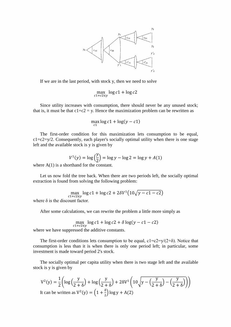
If we are in the last period, with stock y, then we need to solve

max𝑐1+𝑐2≤𝑦

log 𝑐1 + log 𝑐2

Since utility increases with consumption, there should never be any unused stock;

that is, it must be that c1+c2 = y. Hence the maximization problem can be rewritten as

max𝑐1

log 𝑐1 + log(𝑦 − 𝑐1)

The first-order condition for this maximization lets consumption to be equal,

c1=c2=y/2. Consequently, each player's socially optimal utility when there is one stage

left and the available stock is y is given by

𝑉1(𝑦) = log (𝑦

2) = log 𝑦 − log 2 = log 𝑦 + 𝐴(1)

where A(1) is a shorthand for the constant.

Let us now fold the tree back. When there are two periods left, the socially optimal

extraction is found from solving the following problem:

max𝑐1+𝑐2≤𝑦

log 𝑐1 + log 𝑐2 + 2𝛿𝑉1(10√𝑦 − 𝑐1 − 𝑐2)

where δ is the discount factor.

After some calculations, we can rewrite the problem a little more simply as

max

𝑐1+𝑐2≤𝑦log 𝑐1 + log 𝑐2 + 𝛿 log(𝑦 − 𝑐1 − 𝑐2)

where we have suppressed the additive constants.

The first-order conditions lets consumption to be equal, c1=c2=y/(2+δ). Notice that

consumption is less than it is when there is only one period left; in particular, some

investment is made toward period 2's stock.

The socially optimal per capita utility when there is two stage left and the available

stock is y is given by

V2(y) =1

2(log (

y

2 + δ) + log (

y

2 + δ) + 2δV1 (10√y − (

y

2 + δ) − (

y

2 + δ)))

It can be written as V2(y) = (1 +δ

2) log y + A(2)

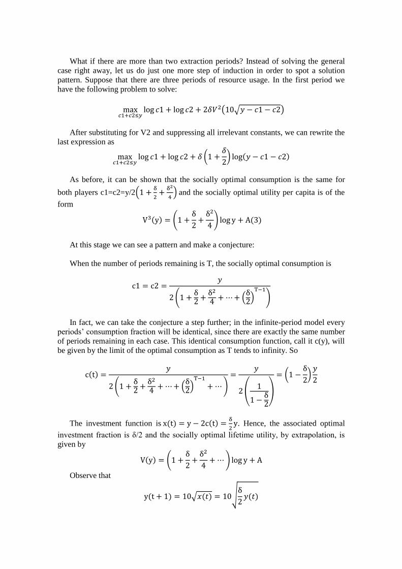
What if there are more than two extraction periods? Instead of solving the general

case right away, let us do just one more step of induction in order to spot a solution

pattern. Suppose that there are three periods of resource usage. In the first period we

have the following problem to solve:

max𝑐1+𝑐2≤𝑦

log 𝑐1 + log 𝑐2 + 2𝛿𝑉2(10√𝑦 − 𝑐1 − 𝑐2)

After substituting for V2 and suppressing all irrelevant constants, we can rewrite the

last expression as

max𝑐1+𝑐2≤𝑦

log 𝑐1 + log 𝑐2 + 𝛿 (1 +𝛿

2) log(𝑦 − 𝑐1 − 𝑐2)

As before, it can be shown that the socially optimal consumption is the same for

both players c1=c2=y/2(1 +δ

2+

δ2

4) and the socially optimal utility per capita is of the

form

V3(y) = (1 +δ

2+

δ2

4) log y + A(3)

At this stage we can see a pattern and make a conjecture:

When the number of periods remaining is T, the socially optimal consumption is

c1 = c2 =𝑦

2 (1 +δ2 +

δ2

4 + ⋯ + (δ2)

T−1

)

In fact, we can take the conjecture a step further; in the infinite-period model every

periods’ consumption fraction will be identical, since there are exactly the same number

of periods remaining in each case. This identical consumption function, call it c(y), will

be given by the limit of the optimal consumption as T tends to infinity. So

c(t) =𝑦

2 (1 +δ2 +

δ2

4 + ⋯ + (δ2)

T−1

+ ⋯ )

=𝑦

2 (1

1 −δ2

)

= (1 −δ

2)

𝑦

2

The investment function is x(t) = y − 2c(t) =δ

2y. Hence, the associated optimal

investment fraction is δ/2 and the socially optimal lifetime utility, by extrapolation, is

given by

V(y) = (1 +δ

2+

δ2

4+ ⋯ ) log y + A

Observe that

y(t + 1) = 10√𝑥(𝑡) = 10√δ

2𝑦(𝑡)

So, the socially optimal sustainable resource stock is 100δ

2 (equation fixed point)

Note See an explanation of the social optimum in Dutta’s book

Game Equilibrium

Suppose that the two players are extracting the resource unilaterally. Each player

will then only consider her own utility and seek to pick extraction rates that maximize

this utility. . We will assume that if the desired consumptions add up to an amount

greater than the available stock, then, the stack is divided equally between the two

players. Like the social optimum, the game equilibrium can also be solved by backward

induction.

As a start, suppose that there are exactly two periods and we are in the last period

with stock y. Since utility increases in the amount of consumption and there are no more

periods afterward, each player will attempt to consume everything. Hence, the stage-

game equilibrium is one where each player's actual consumption is c1=c2=y/2.

Consequently, each player's equilibrium utility is given by

𝑊1(𝑦) = log (𝑦

2) = log 𝑦 + 𝐵(1)

Let us now fold the tree back. When there are two periods left, if players are

expected to consume c1=θ1y and c2=θ2y, where θi is the fraction of the resource

consumed in the first period, then, player 1 faces the following best-response problem

max𝜃1

log 𝜃1𝑦 + 𝛿𝑊1(10√𝑦 − 𝜃1𝑦 − 𝜃2𝑦)

This problem can be written equivalently as

max𝜃1

log 𝜃1 +𝛿

2log(1 − 𝜃1 − 𝜃2)

It can be shown that the best-response fraction of consumption is

𝜃1 = 𝑏(𝜃2) =1 − 𝜃2

1 +𝛿2

In an equilibrium, θ1 = b(θ2) and θ2 = b(θ1), and it can be shown that each player

chooses the same extraction rate (symmetric equilibrium), and that this rate is

θ1 = θ2 =1

2 +δ2

The equilibrium utility when there are two remaining periods can be written as

𝑊2(𝑦) = (1 +𝛿

2) log 𝑦 + 𝐵(2)

It can be shown that when there are T periods left the equilibrium extraction rate is

𝜃1 = 𝜃2 =1

2 +𝛿2 + ⋯ + (

𝛿2)

T−1

In the infinite-period model, the equilibrium consumption function, call it c*(y)=θy,

will be given by the limit of the equilibrium consumption as T tends to infinity

c∗(y) =1

2 +𝛿2 + ⋯ + (

𝛿2)

T−1

+ ⋯

y =1 −

𝛿2

2 −𝛿2

y

The investment function is x(t) = y − 2c ∗ (t) =δ

4−δy.

So, y(t + 1) = 10√𝑥(𝑡) = 10√δ

4−δ𝑦(𝑡) and the equilibrium sustainable resource

stock is 100δ

4−δ (equation fixed point)

Note See an explanation of the game equilibrium in Dutta’s book

Comparison of the Socially Optimal and the Equilibrium Outcomes

The general lesson is that unilateral extraction leads to over-extraction; consumption

in the equilibrium solution is higher than in the socially optimal solution. The socially

optimal function c(y) is always lower than the equilibrium function c*(y)

c(t) =1 −

δ2

2𝑦 <

1 −𝛿2

2 −𝛿2

y = c∗(y)

The intuition for this conclusion is precisely that in the equilibrium solution a player

only collects a part of his action's consequences. Hence, he is more likely to over-

extract because part of the burden of that overconsumption is borne by a lowering of the

other player's future consumption.

Consider two different societies, one in which consumption is socially managed and

another in which it is unilaterally determined. Imagine that both societies start with the

same resource stock. By period 2, the first society would have a larger resource stock

because it invested more in the first period. This increase implies in turn that this

society would again have a larger investment level in period 2. This result would occur

for two reasons; first, society 1 in any case invests a larger fraction of any resource

stock. Second, it has a larger resource stock available.

Now, the continuation of this logic is also clear. In each period the socially managed

society would have a larger resource stock, would invest more, and hence would

continue to have a larger resource stock in the future. If yt denotes the resource stock in

the socially managed situation and yt’ denotes the equilibrium stock, then yt > yt’ for all

periods t> 1 even though y1=y1’.

Another consequence of this argument is that the sustainable socially optimal stock

is higher than the achievable equilibrium stock. A sustainable stock is one that keeps

getting regenerated; that is, it is a level at which y(t+1)=y(t) in all periods. At the

sustainable socially optimal stock, y∗ =100δ

2, socially optimal investment x(y*) exactly

regenerates that stock, that is, y∗ = 10√x(y∗). This stock is not achievable in

equilibrium because the equilibrium investment at y* is less than x(y*). In fact, the

achievable equilibrium stock 100δ

4−δ is lower.

General Dynamic Games

There are three conclusions that we have seen in the commons model. First,

although in the finite-horizon game each player also looks at how many periods of

extraction remain in order to make this choice, in the infinite-horizon there is an

equilibrium in which each player looks only at the size of the current resource stock, or

game environment, to decide how much to consume. Such strategies have a technical

name; they are called Markovian strategies, and an equilibrium in these strategies is

called a Markov perfect equilibrium (MPE).

Markovian strategies are attractive because of their simplicity; they do not require a

player to keep track of either what his opponent did in the past or how the resource has

evolved in previous periods. If the number of game environments is finite, MPE always

exists. When the environment can be any one of an infinite number, although some

games such as our commons model do have MPE, we do not know whether there is

always an MPE. In a repeated game, there is only one environment; hence a Markovian

strategy is the same thing as choosing the same action over and over again. An MPE,

therefore, is the same thing as playing a stage-game Nash equilibrium repeatedly.

Unlike a dynamic game, therefore, MPEs in repeated games do not lead to any

interesting time patterns of behavior.

The second conclusion of our model is that there is a unique equilibrium (that looks

similar to the socially optimal solution). This conclusion is not at all robust. In general

dynamic games, there are many MPEs. When we additionally consider strategies that

look like the trigger strategies of repeated games, we generate yet more equilibria.

The final conclusion was that equilibrium is socially suboptimal; too much of the

resource is extracted and hence equilibrium utilities are lower than socially optimal

utilities. Unless the threat of punishment is imposed, this conclusion holds in repeated

games and in a variety of dynamic games. Using logic similar to that of repeated games,

it is also possible to show that trigger like strategies can sometimes remedy this problem

in a dynamic game. If players believe that good behavior will be rewarded and bad

behavior punished in the future, they might be inclined to behave themselves

Theme 13: Games with Incomplete Information

background In imperfect information games a player can be unaware of actions taken

by other players, either in the past or contemporaneously. However, a player always

knows the answers to such questions as: Who are the other players? What are their

strategies? What are their preferences? And so on. Incomplete information games

include situations where a player is unsure about the answer to some or all of those

questions.

Recall the Battle of the Sexes game. Husband (H) and wife (W) have to decide whether

to go to a football game (F) or to the opera (O). They would rather be together than

apart, but the husband prefers that they go to F together while his wife prefers they go to

O together.

Suppose now that the husband is not sure of his wife's preferences. In particular, he does

not know if his wife likes to be with him (loving) or if she prefers to go to either event

by herself (leaving). In other words, he is unaware whether her preferences are the

standard preferences, or whether they are given by the new table.

Husband \ Wife

(loving)

football opera

football 3,1 0,0

opera 0,0 1,3

Husband \ Wife

(leaving)

football opera

football 3,0 0,1

opera 0,3 1,0

In this example, the incompleteness has been about player 2's preferences, and there

were just two possible preferences in each case. In general, there may be

incompleteness about player 1's preferences as well, and there may be many possible

preferences. As you might suspect, all that happens is that the number of payoff

matrices increases with the types of incompleteness. Also, this example suggests a

definition: a game of incomplete information is one in which players do not know some

relevant characteristics of their opponents, which may include their payoffs, their

available options, and even their beliefs.

Three assumptions underlie the example:

Assumption 1: The wife knows her preferences; that is, she knows which table is the

right one.

Assumption 2: The husband does not know his wife's real preferences; he attaches a

probability r to the fact that her true preferences are given by the first table (and

therefore a probability 1 - r to the other table).

Assumption 3: The wife knows her husband's estimate of her preferences; that is, she

knows the value of r.

Of the three assumptions surely the most controversial is the last one. It goes by the

name of the assumption of a common prior. What this means precisely is that there is a

common estimate that both players have about what is known to be unknown. One

interpretation is that in the larger population of players who could be cast in the role of a

"wife" a fraction r like to be with their husbands, and this fact is commonly known.

The further information that any specific wife has is knowing which part of the

population she herself belongs to.

Let us turn to equilibrium analysis. In three papers written in 1967 and 1968,4 John

Harsanyi proposed a generalization of Nash equilibrium that is appropriate for an

incomplete information game. Harsanyi's proposal was in two parts.

First, turn the game of incomplete information into a game of imperfect information.

To do so, reinterpret the game as follows: an artificial player "nature" picks from the

two possible player preferences or "types" the true preference or type of player 2 (and

informs the wife but not the husband of this choice). The corresponding extensive form

is therefore as displayed in Dutta’s Figure 20.1.

Now all players have the same ex ante knowledge, that is, that it is a game of complete

information; ex post, the husband does not know nature's move although the wife does.

In any game of imperfect information, an appropriate equilibrium concept is Nash

equilibrium and we use it here.

Second, use Nash equilibrium (of this imperfect information version) as the solution

concept.

In incomplete information games, Nash equilibrium is given a special name; it is called

a Bayes-Nash equilibrium. We will now compute Bayes-Nash equilibria in the example.

Note that a pure strategy for the husband is a choice of F or O; a mixed strategy is the

choice of a probability on F (and denote this probability p). A strategy for the wife is a

pair; its first component is the choice that a wife with the first set of preferences will

make (call her a type 1 wife) and the second component is a type 2 wife's choice. Hence

a pure strategy for the wife is one of the four pairs (F, F), (F, O), (O, F), and (O, O), and

a mixed strategy is a pair (m1, m2), where mi is the probability that the type i wife will

play F.

Definition. A Bayes-Nash equilibrium of the game is a triple (l, m1, m2) in which each

player (and each type of player) plays a best response, as follows:

(1) The probability mi maximizes a type i wife's payoffs if the husband selects F with

probability l. This holds for both i = 1 and 2.

(2) The probability l maximizes the husband's expected payoffs if he believes that with

probability r he will encounter a type 1 wife who will play F with probability m1 (while

with probability 1 - r he will encounter a type 2 wife who will play F with probability

m2).

Pure-Strategy Bayes-Nash Equilibria

Suppose that the husband plays F for sure, that is, that p = 1. In a best response, a type 1

wife must play F, and conversely, a type 2 wife must play O (i.e., m1 = 1, m2 = 0). The

only remaining question is whether or not the husband maximizes his expected payoffs

by playing F [against (F, O)]. By playing F, he gets an expected payoff of 3r (since he

gets 3 by playing against the type I wife and 0 against the type 2 wife and the former

has probability r). By the same logic, by playing O, the husband gets an expected payoff

of 1 - r. Evidently, F is a best response if 3r≥1 - r, or equivalently if r≥1/4. Hence, if the

likelihood of the wife being of type I is at least 25 percent, then it is a Bayes-Nash

equilibrium for the husband to play F while the wives play (F, O).

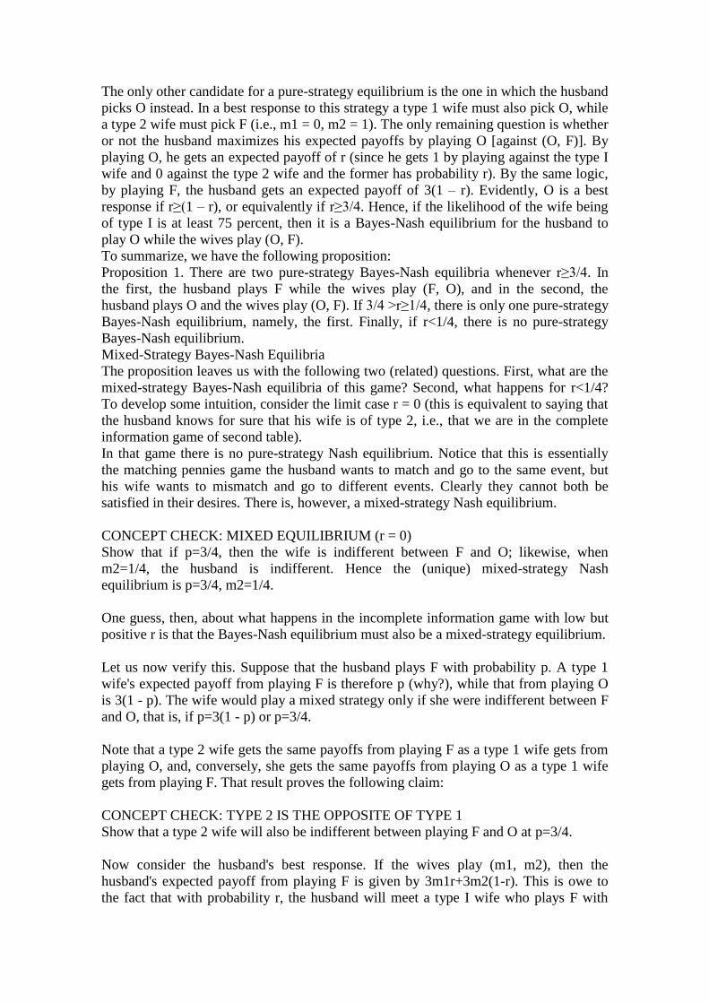
The only other candidate for a pure-strategy equilibrium is the one in which the husband

picks O instead. In a best response to this strategy a type 1 wife must also pick O, while

a type 2 wife must pick F (i.e., m1 = 0, m2 = 1). The only remaining question is whether

or not the husband maximizes his expected payoffs by playing O [against (O, F)]. By

playing O, he gets an expected payoff of r (since he gets 1 by playing against the type I

wife and 0 against the type 2 wife and the former has probability r). By the same logic,

by playing F, the husband gets an expected payoff of 3(1 – r). Evidently, O is a best

response if r≥(1 – r), or equivalently if r≥3/4. Hence, if the likelihood of the wife being

of type I is at least 75 percent, then it is a Bayes-Nash equilibrium for the husband to

play O while the wives play (O, F).

To summarize, we have the following proposition:

Proposition 1. There are two pure-strategy Bayes-Nash equilibria whenever r≥3/4. In

the first, the husband plays F while the wives play (F, O), and in the second, the

husband plays O and the wives play (O, F). If 3/4 >r≥1/4, there is only one pure-strategy

Bayes-Nash equilibrium, namely, the first. Finally, if r<1/4, there is no pure-strategy

Bayes-Nash equilibrium.

Mixed-Strategy Bayes-Nash Equilibria

The proposition leaves us with the following two (related) questions. First, what are the

mixed-strategy Bayes-Nash equilibria of this game? Second, what happens for r<1/4?

To develop some intuition, consider the limit case r = 0 (this is equivalent to saying that

the husband knows for sure that his wife is of type 2, i.e., that we are in the complete

information game of second table).

In that game there is no pure-strategy Nash equilibrium. Notice that this is essentially

the matching pennies game the husband wants to match and go to the same event, but

his wife wants to mismatch and go to different events. Clearly they cannot both be

satisfied in their desires. There is, however, a mixed-strategy Nash equilibrium.

CONCEPT CHECK: MIXED EQUILIBRIUM (r = 0)

Show that if p=3/4, then the wife is indifferent between F and O; likewise, when

m2=1/4, the husband is indifferent. Hence the (unique) mixed-strategy Nash

equilibrium is p=3/4, m2=1/4.

One guess, then, about what happens in the incomplete information game with low but

positive r is that the Bayes-Nash equilibrium must also be a mixed-strategy equilibrium.

Let us now verify this. Suppose that the husband plays F with probability p. A type 1

wife's expected payoff from playing F is therefore p (why?), while that from playing O

is 3(1 - p). The wife would play a mixed strategy only if she were indifferent between F

and O, that is, if p=3(1 - p) or p=3/4.

Note that a type 2 wife gets the same payoffs from playing F as a type 1 wife gets from

playing O, and, conversely, she gets the same payoffs from playing O as a type 1 wife

gets from playing F. That result proves the following claim:

CONCEPT CHECK: TYPE 2 IS THE OPPOSITE OF TYPE 1

Show that a type 2 wife will also be indifferent between playing F and O at p=3/4.

Now consider the husband's best response. If the wives play (m1, m2), then the

husband's expected payoff from playing F is given by 3m1r+3m2(1-r). This is owe to

the fact that with probability r, the husband will meet a type I wife who plays F with

probability ml in which case, the husband's payoff is 3, and plays O with probability 1 -

m1, and then the husband's payoff is 0. Add to this payoff the fact that, with probability

1 - r, the husband will meet a type 2 wife who plays F with probability m2 yielding the

husband a payoff of 3 and plays O with probability 1 - m2 yielding the husband a payoff

of 0.

By the same logic, the husband's expected payoff from playing O is given by the

expression (1-m1)r+(1-m2)(1-r).

If the expression in first equation exceeds the expression in second equation, the

husband strictly prefers F to O (and vice versa if first equation is less than second

equation). The husband is indifferent only if the two expressions are equal; in this case,

both F and O are best responses and any mixture between them in particular, is a best

response. After collecting terms, the two expected payoffs are seen to be equal if and

only if

(4m1-1) r= (1-4m2) (1-r)

Provided the mixed strategies (m1, m2) satisfy this equation, the husband has a mixed-

strategy best response and in particular a best response p=3/4. When the husband plays

p=3/4, in turn, any mixed strategy pair (m1, m2) is a best response for the wives in

particular, the (m1, m2) given by the equation.

Summarizing all this, we have proved the following proposition:

Proposition 2. Regardless of the value of r, there is always a mixed-strategy Bayes-Nash

equilibrium; in particular, p=3/4 m1=1/4 m2=1/4. There may be additional mixed-

strategy Bayes-Nash equilibria, and these are characterized by p=3/4, and (ml, m2) that

satisfy the equation.

What we learned in this section is that in a Bayes-Nash equilibrium, the informed player

chooses a strategy based on her information, and consequently this choice can be

different for different types of this player. The uninformed player realizes that different

types will play different strategies; that is, he realizes that he is in effect facing a mixed

strategy with the probability weights in the mixture given by the odds on the different

types. He therefore has to choose the best response to this mixed strategy. An

equilibrium occurs when no type of informed player or the uninformed player wishes to

alter her strategy choice.