gas viscosity at high pressure and high...
TRANSCRIPT

GAS VISCOSITY AT HIGH PRESSURE AND HIGH TEMPERATURE
A Dissertation
by
KEGANG LING
Submitted to the Office of Graduate Studies of Texas A&M University
in partial fulfillment of the requirements for the degree of
DOCTOR OF PHILOSOPHY
December 2010
Major Subject: Petroleum Engineering

GAS VISCOSITY AT HIGH PRESSURE AND HIGH TEMPERATURE
A Dissertation
by
KEGANG LING
Submitted to the Office of Graduate Studies of Texas A&M University
in partial fulfillment of the requirements for the degree of
DOCTOR OF PHILOSOPHY
Approved by:
Co-Chairs of Committee, Gioia Falcone Catalin Teodoriu
Committee Members, William D. McCain Jr. Yuefeng Sun
Head of Department, Stephen A. Holditch
December 2010
Major Subject: Petroleum Engineering

iii
ABSTRACT
Gas Viscosity at High Pressure and High Temperature. (December 2010)
Kegang Ling, B. S., University of Petroleum, China;
M. S., University of Louisiana at Lafayette
Chair of Advisory Committee: Dr. Gioia Falcone
Gas viscosity is one of the gas properties that is vital to petroleum engineering. Its role in
the oil and gas production and transportation is indicated by its contribution in the
resistance to the flow of a fluid both in porous media and pipes. Although viscosity of
some pure components such as methane, ethane, propane, butane, nitrogen, carbon
dioxide and binary mixtures of these components at low-intermediate pressure and
temperature had been studied intensively and been understood thoroughly, very few
investigations were performed on viscosity of naturally occurring gases, especially gas
condensates at low-intermediate pressure and temperature, even fewer lab data were
published. No gas viscosity data at high pressures and high temperatures (HPHT) is
available. Therefore this gap in the oil industry still needs to be filled.
Gas viscosity at HPHT becomes crucial to modern oil industry as exploration and
production move to deep formation or deep water where HPHT is not uncommon.
Therefore, any hydrocarbon encountered there is more gas than oil due to the chemical
reaction causing oil to transfer to gas as temperature increases. We need gas viscosity to
optimize production rate for production system, estimate reserves, model gas injection,
design drilling fluid, and monitor gas movement in well control. Current gas viscosity
correlations are derived using measured data at low-moderate pressures and
temperatures, and then extrapolated to HPHT. No measured gas viscosities at HPHT are

iv
available so far. The validities of these correlations for gas viscosity at HPHT are
doubted due to lack of experimental data.
In this study, four types of viscometers are evaluated and their advantages and
disadvantages are listed. The falling body viscometer is used to measure gas viscosity at
a pressure range of 3000 to 25000 psi and a temperature range of 100 to 415 oF.
Nitrogen viscosity is measured to take into account of the fact that the concentration of
nonhydrocarbons increase drastically in HPHT reservoir. More nitrogen is found as we
move to HPHT reservoirs. High concentration nitrogen in natural gas affects not only the
heat value of natural gas, but also gas viscosity which is critical to petroleum
engineering. Nitrogen is also one of common inject gases in gas injection projects, thus
an accurate estimation of its viscosity is vital to analyze reservoir performance. Then
methane viscosity is measured to honor that hydrocarbon in HPHT which is almost pure
methane. From our experiments, we found that while the Lee-Gonzalez-Eakin
correlation estimates gas viscosity at a low-moderate pressure and temperature
accurately, it cannot give good match of gas viscosity at HPHT. Apparently, current
correlations need to be modified to predict gas viscosity at HPHT. New correlations
constructed for HPHT conditions based on our experiment data give more confidence on
gas viscosity.

v
DEDICATION
To my family for their love and support

vi
ACKNOWLEDGMENTS
During these four years at Texas A&M University I have tried my best to adhere to the
requirements of being a qualified graduate student. I got tons of help in the process of
pursuing my Ph.D. degree. I want to acknowledge these people for their generosity and
kindness.
First of all, my gratitude goes to my advisors, Dr. Gioia Falcone and Dr. Catalin
Teodoriu, for their veritable academic advice to me in these years, and in years to come.
Their inspiration, encouragement, guardianship, and patience were essential for my
research and study.
I would also like to express my sincere appreciation to my committee member, Dr.
William D. McCain Jr., for his advice, knowledge, and priceless assistance during these
years.
Thanks are also extended to a member of my supervising committee, Dr. Yuefeng Sun,
of the Department of Geology and Geophysics, for managing time out of his busy
schedule to provide valuable comments and suggestions.
Furthermore, I appreciate Dr. Catalin Teodoriu, Dr. William D. McCain Jr., and Mr.
Anup Viswanathan for setting up the High Pressure High Temperature laboratory for
this project, and Mr. John Maldonado, Sr. for supplying gas resources. I am grateful to
the sponsors of the Crisman Petroleum Research Institute at Texas A&M University for
providing funding for this project.
I wish to express my appreciation to the faculty and staff of the Department of Petroleum

vii
Engineering at Texas A&M University. I am indebted to my colleagues because they
made the whole study more enjoyable. I truly appreciate my family, without their
support I would not have realized my dream.

viii
TABLE OF CONTENTS
Page
ABSTRACT ................................................................................................................... iii
DEDICATION ...............................................................................................................v
ACKNOWLEDGMENTS..............................................................................................vi
TABLE OF CONTENTS ...............................................................................................viii
LIST OF TABLES .........................................................................................................x
LIST OF FIGURES........................................................................................................xii
1.1 Viscosity.............................................................................................................1 1.2 Role of Gas Viscosity in Petroleum Engineering...............................................4 1.3 Methods to Get Gas Viscosity............................................................................5
2.1 Gas Viscosity Measuring Instrument .................................................................7 2.2 Gas Viscosity Experimental Data ......................................................................29 2.3 Available Gas Viscosity Correlations ................................................................47
4.1 Experiment Facility ............................................................................................78 4.2 Experiment Procedure ........................................................................................86 4.3 Measurement Principle of Viscometer in This Study ........................................89 4.4 Calibration of Experimental Data ......................................................................109
5.1 Nitrogen Viscosity Measurement.......................................................................125
CHAPTER I INTRODUCTION .............................................................................1
CHAPTER II LITERATURE REVIEW...................................................................7
CHAPTER III OBJECTIVE .......................................................................................77
CHAPTER IV METHODOLOGY .............................................................................78
CHAPTER V EXPERIMENTAL RESULTS............................................................125

ix
Page
5.2 Nitrogen Viscosity Analysis...............................................................................126 5.3 Methane Viscosity Measurement .......................................................................134 5.4 Methane Viscosity Analysis...............................................................................136
6.1 Nitrogen Viscosity Correlation ..........................................................................141 6.2 Methane Viscosity Correlation...........................................................................154
7.1 Conclusions ........................................................................................................176 7.2 Recommendations ..............................................................................................176
NOMENCLATURE.......................................................................................................177
REFERENCES...............................................................................................................183
APPENDIX A ................................................................................................................191
APPENDIX B ................................................................................................................205
VITA ..............................................................................................................................224
CHAPTER VI NEW GAS VISCOSITY CORRELATIONS .....................................141
CHAPTER VII CONCLUSIONS AND RECOMMENDATIONS..............................176

x
LIST OF TABLES
Page
Table 1-1. Examples of HPHT fields ....................................................................... 5
Table 2-1. Methane viscosity collected by Lee (1965) ............................................ 34
Table 2-2. Methane viscosity by Diehl et al. (1970) ................................................ 35
Table 2-3. Methane viscosity by Stephan and Lucas (1979) ................................... 36
Table 2-4. Methane viscosity by Golubev (1959) .................................................... 38
Table 2-5. Nitrogen viscosity collected by Stephan and Lucas (1979) .................... 39
Table 2-6. Viscosity-temperature-pressure data used for Comings-Mayland-Egly (1940, 1944) correlation ................................. 51
Table 2-7. Viscosity-temperature-pressure data used for
Smith-Brown (1943) correlation ............................................................ 52 Table 2-8. Viscosity-temperature-pressure data used for
Bicher-Katz (1943) correlation .............................................................. 54 Table 2-9. Viscosity-temperature-pressure data used for
Carr-Kobayashi-Burrrow (1954) correlation.......................................... 59 Table 2-10. Viscosity-temperature-pressure data used for
Jossi-Stiel-Thodos (1962) correlation .................................................... 63 Table 2-11. Viscosity-temperature-pressure data used for
Lee-Gonzalez-Eakin (1970) correlation ................................................. 66 Table 2-12. Composition of eight natural gas samples (Gonzalez et al., 1970) ......... 67
Table 4-1. The dimension of chamber and piston (Malaguti and Suitter, 2010) ..... 90
Table 4-2. Pressure-corrected nitrogen viscosity ..................................................... 118

xi
Page
Table 4-3. Nitrogen viscosity from NIST ............................................................... 119
Table 4-4. Pressure-corrected methane viscosity .................................................... 120
Table 4-5. Methane viscosity from NIST ................................................................ 121
Table 5-1. Statistic of nitrogen viscosity experiment in this study ......................... 126
Table 5-2. Error analysis for nitrogen viscosity from NIST program ..................... 134
Table 5-3. Statistic of methane viscosity experiment in this study ......................... 135
Table 5-4. Error analysis for methane viscosity from different correlations .......... 140
Table 6-1. Data used to develop nitrogen viscosity correlation .............................. 143
Table 6-2. Absolute error by comparing nitrogen viscosity data with values from correlation ........................................................................... 147
Table 6-3. Relative error by comparing nitrogen viscosity data with
values from correlation ........................................................................... 151 Table 6-4. Data used to develop new methane viscosity correlation ....................... 156 Table 6-5. Absolute error by comparing methane viscosity data with
values from correlation ........................................................................... 164 Table 6-6. Relative error analysis by comparing methane viscosity
data with values from correlation ........................................................... 170

xii
LIST OF FIGURES
Page
Figure 1-1. Laminar shear in fluids, after Wikipedia viscosity (2010) ..................... 1 Figure 1-2. Laminar shear of a fluid film. ................................................................. 2 Figure 1-3. Laminar shear of for non-Newtonian fluids flow,
after Wikipedia viscosity (2010) ............................................................ 4 Figure 2-1. Schematic of fluid flow through a pipe .................................................. 8 Figure 2-2. Fluid flow profile in a circular pipe ........................................................ 9 Figure 2-3. Cross section view of a circular pipe ...................................................... 11 Figure 2-4. Capillary viscometer in two positions, after Rankine (1910) ................. 18 Figure 2-5. A classic capillary viscometer, after Rankine (1910). ............................ 20 Figure 2-6. Cross section of falling cylinder viscometer body and
ancillary components, after Chan and Jckson (1985)............................. 21 Figure 2-7. Cross section of a falling ball viscometer body,
after Florida Atlantic University (2005) ................................................. 23 Figure 2-8. Cross section of a falling needle viscometer body,
after Park (1994). .................................................................................... 24 Figure 2-9. Rolling ball viscometer, after Tomida et al. (2005). .............................. 25 Figure 2-10. Vibrational viscometer employed tuning fork technology,
after Paul N. Gardner Co. (2010). .......................................................... 26 Figure 2-11. An oscillating sphere system for creating controlled
amplitude in liquid, after Steffe (1992). ................................................. 27 Figure 2-12. Vibrating rod system for measuring dynamic viscosity,
after Steffe (1992). ................................................................................. 28

xiii
Page
Figure 2-13. Viscosity ratio versus reduced pressure charts used to estimate gas viscosity, after Comings and Egly (1940). ........................ 48
Figure 2-14. Viscosity ratio versus reduced temperature,
after Comings et al. (1944). .................................................................... 49 Figure 2-15. Viscosity ratio versus reduced pressure,
after Comings et al. (1944). .................................................................... 50 Figure 2-16. Viscosity correlation for normal paraffins,
after Smith and Brown (1943). ............................................................... 53 Figure 2-17. Viscosity of paraffin hydrocarbons at high-reduced
temperatures (top) and at low-reduced temperatures (bottom), after Bicher and Katz (1943). ................................................................. 55
Figure 2-18. Viscosity ratio versus pseudo-reduced pressure,
after Carr et al. (1954). ........................................................................... 56 Figure 2-19. Viscosity ratio versus pseudo-reduced temperature,
after Carr et al. (1954). ........................................................................... 57 Figure 2-20. Relationship between the residual viscosity modulus ( )ξμμ *−g
and reduced density rρ for normally behaving substances, after Jossi et al. (1962). .......................................................................... 62
Figure 2-21. Relationship between the residual viscosity modulus ( )ξμμ *−g
and reduced density rρ for the substances investigated, after Jossi et al. (1962). .......................................................................... 62
Figure 2-22. Comparisons of CH4 (top) and N2 (bottom) densities
between NIST values and lab data. ........................................................ 70 Figure 2-23. Comparisons of CH4 (top) and N2 (bottom) viscosities
between NIST value and lab data ........................................................... 71 Figure 4-1. The setup of apparatus for this study ...................................................... 78 Figure 4-2. Schematic of experimental facility ......................................................... 79

xiv
Page
Figure 4-3. Gas booster system used to compress gas in this study .......................... 80 Figure 4-4. The temperature control system in this study ......................................... 83 Figure 4-5. Schematic of the measurement system in this study .............................. 84 Figure 4-6. Recording control panel to control the experiment ................................ 86 Figure 4-7. Contaminants trapped on the piston ....................................................... 87 Figure 4-8. Piston moves inside of chamber of viscometer using in this study ........ 89 Figure 4-9. Representing the annulus as a slot: (a) annulus and
(b) equivalent slot, after Bourgoyne et al. (1986) .................................. 94 Figure 4-10. Free body diagram for controlled fluid volume in a slot,
after Bourgoyne et al. (1986) ................................................................. 94 Figure 4-11. Schematic of fluid flow through an annulus
between piston and chamber. ................................................................. 99 Figure 4-12. Friction factor vs. particle Reynolds number for
particles of different sphericities (Bourgoyne et al., 1986). ................... 104 Figure 4-13. Comparison of raw viscosity data with NIST values for
methane at temperature of 100 oF........................................................... 110 Figure 4-14. Comparison of raw viscosity data with NIST values for
methane at temperature of 250 oF........................................................... 111 Figure 4-15. Comparison of raw viscosity data with NIST values for
nitrogen at temperature of 152 oF ........................................................... 111 Figure 4-16. Comparison of raw viscosity data with NIST values for
nitrogen at temperature of 330 oF ........................................................... 112 Figure 4-17. Comparison of pressure-converted methane viscosity
with NIST values at temperature of 100 oF ............................................ 113 Figure 4-18. Comparison of pressure-converted methane viscosity
with NIST values at temperature of 250 oF ............................................ 113

xv
Page
Figure 4-19. Comparison of pressure-converted nitrogen viscosity with NIST values at temperature of 152 oF ............................................ 114
Figure 4-20. Comparison of pressure-converted nitrogen viscosity
with NIST values at temperature of 330 oF ............................................ 114 Figure 4-21. Comparison of pressure-temperature-converted methane
viscosity with NIST values at temperature of 100 oF ............................. 122 Figure 4-22. Comparison of pressure-temperature-converted methane
viscosity with NIST values at temperature of 250 oF ............................. 123 Figure 4-23. Comparison of pressure-temperature-converted nitrogen
viscosity with NIST values at temperature of 152 oF ............................. 123 Figure 4-24. Comparison of pressure-temperature-converted nitrogen
viscosity with NIST values at temperature of 330 oF ............................. 124 Figure 5-1. Nitrogen viscosity vs. pressure at 116 oF (Test 68) ................................ 127 Figure 5-2. Nitrogen viscosity vs. pressure at 116 oF (Test 69) ................................ 127 Figure 5-3. Nitrogen viscosity vs. pressure at 116 oF (Test 70) ................................ 128 Figure 5-4. Nitrogen viscosity vs. pressure at 116 oF (Test 71) ................................ 128 Figure 5-5. Lee-Gonzalez-Eakin correlation is inappropriate for
nitrogen viscosity at temperature of 116 oF ........................................... 130 Figure 5-6. Lee-Gonzalez-Eakin correlation is inappropriate for
nitrogen viscosity at temperature of 220 oF ........................................... 131 Figure 5-7. Lee-Gonzalez-Eakin correlation is inappropriate for
nitrogen viscosity at temperature of 300 oF ........................................... 131 Figure 5-8. Lee-Gonzalez-Eakin correlation is inappropriate for
nitrogen viscosity at temperature of 350 oF ........................................... 132 Figure 5-9. Comparison between new correlation and NIST values
at temperature of 116 oF ......................................................................... 132

xvi
Page
Figure 5-10. Comparison between new correlation and NIST values at temperature of 200 oF ......................................................................... 133
Figure 5-11. Comparison between new correlation and NIST values
at temperature of 300 oF ......................................................................... 133 Figure 5-12. Comparison between new correlation and NIST values
at temperature of 350 oF ......................................................................... 134 Figure 5-13. Methane viscosity vs. pressure at 100 oF (Test 50) ................................ 136 Figure 5-14. Methane viscosity vs. pressure at 100 oF (Test 51) ................................ 137 Figure 5-15. Comparison this study with existing correlations
at temperature of 100 oF ......................................................................... 138 Figure 5-16. Comparison this study with existing correlations
at temperature of 200 oF ......................................................................... 139 Figure 5-17. Comparison this study with existing correlations
at temperature of 300 oF ......................................................................... 139 Figure 5-18. Comparison this study with existing correlations
at temperature of 415 oF ......................................................................... 140 Figure A - 1. Nitrogen viscosity vs. pressure at 134 oF (Test 72) ................................ 191
Figure A - 2. Nitrogen viscosity vs. pressure at 134 oF (Test 73) ................................ 192
Figure A - 3. Nitrogen viscosity vs. pressure at 134 oF (Test74) ................................. 192
Figure A - 4. Nitrogen viscosity vs. pressure at 152 oF (Test 75) ................................ 193
Figure A - 5. Nitrogen viscosity vs. pressure at 152 oF (Test 76) ................................ 193
Figure A - 6. Nitrogen viscosity vs. pressure at 152 oF (Test 77) ................................ 194
Figure A - 7. Nitrogen viscosity vs. pressure at 170 oF (Test 78) ................................ 194
Figure A - 8. Nitrogen viscosity vs. pressure at 170 oF (Test 79) ................................ 195
Figure A - 9. Nitrogen viscosity vs. pressure at 170 oF (Test 80) ................................ 195

xvii
Page
Figure A - 10. Nitrogen viscosity vs. pressure at 170 oF (Test 81) ................................ 196
Figure A - 11. Nitrogen viscosity vs. pressure at 200 oF (Test 82) ................................ 196
Figure A - 12. Nitrogen viscosity vs. pressure at 200 oF (Test 83) ................................ 197
Figure A - 13. Nitrogen viscosity vs. pressure at 250 oF (Test 63) ................................ 197
Figure A - 14. Nitrogen viscosity vs. pressure at 250 oF (Test 64) ................................ 198
Figure A - 15. Nitrogen viscosity vs. pressure at 250 oF (Test 65) ................................ 198
Figure A - 16. Nitrogen viscosity vs. pressure at 250 oF (Test 66) ................................ 199
Figure A - 17. Nitrogen viscosity vs. pressure at 260 oF (Test 67) ................................ 199
Figure A - 18. Nitrogen viscosity vs. pressure at 260 oF (Test 84) ................................ 200
Figure A - 19. Nitrogen viscosity vs. pressure at 260 oF (Test 85) ................................ 200
Figure A - 20. Nitrogen viscosity vs. pressure at 280 oF (Test 86) ................................ 201
Figure A - 21. Nitrogen viscosity vs. pressure at 280 oF (Test 87) ................................ 201
Figure A - 22. Nitrogen viscosity vs. pressure at 300 oF (Test 88) ................................ 202
Figure A - 23. Nitrogen viscosity vs. pressure at 300 oF (Test 89) ................................ 202
Figure A - 24. Nitrogen viscosity vs. pressure at 330 oF (Test 90) ................................ 203
Figure A - 25. Nitrogen viscosity vs. pressure at 330 oF (Test 91) ................................ 203
Figure A - 26. Nitrogen viscosity vs. pressure at 350 oF (Test 92) ................................ 204
Figure A - 27. Nitrogen viscosity vs. pressure at 350 oF (Test 93) ................................ 204
Figure B - 1. Methane viscosity vs. pressure at 120 oF (Test 48) ................................ 205
Figure B - 2. Methane viscosity vs. pressure at 120 oF (Test 49) ................................ 206
Figure B - 3. Methane viscosity vs. pressure at 140 oF (Test 46) ................................ 206

xviii
Page
Figure B - 4. Methane viscosity vs. pressure at 140 oF (Test 47) ................................ 207
Figure B - 5. Methane viscosity vs. pressure at 160 oF (Test 44) ................................ 207
Figure B - 6. Methane viscosity vs. pressure at 160 oF (Test 45) ................................ 208
Figure B - 7. Methane viscosity vs. pressure at 180 oF (Test 42) ................................ 208
Figure B - 8. Methane viscosity vs. pressure at 180 oF (Test 43) ................................ 209
Figure B - 9. Methane viscosity vs. pressure at 188 oF (Test 13) ................................ 209
Figure B - 10. Methane viscosity vs. pressure at 188 oF (Test 14) ................................ 210
Figure B - 11. Methane viscosity vs. pressure at 188 oF (Test 15) ................................ 210
Figure B - 12. Methane viscosity vs. pressure at 200 oF (Test 16) ................................ 211
Figure B - 13. Methane viscosity vs. pressure at 200 oF (Test 17) ................................ 211
Figure B - 14. Methane viscosity vs. pressure at 200 oF (Test 18) ................................ 212
Figure B - 15. Methane viscosity vs. pressure at 220 oF (Test 19) ................................ 212
Figure B - 16. Methane viscosity vs. pressure at 220 oF (Test 20) ................................ 213
Figure B - 17. Methane viscosity vs. pressure at 220 oF (Test 21) ................................ 213
Figure B - 18. Methane viscosity vs. pressure at 225 oF (Test 22) ................................ 214
Figure B - 19. Methane viscosity vs. pressure at 230 oF (Test 23) ................................ 214
Figure B - 20. Methane viscosity vs. pressure at 250 oF (Test 24) ................................ 215
Figure B - 21. Methane viscosity vs. pressure at 250 oF (Test 25) ................................ 215
Figure B - 22. Methane viscosity vs. pressure at 260 oF (Test 26) ................................ 216
Figure B - 23. Methane viscosity vs. pressure at 260 oF (Test 27) ................................ 216
Figure B - 24. Methane viscosity vs. pressure at 280 oF (Test 28) ................................ 217

xix
Page
Figure B - 25. Methane viscosity vs. pressure at 280 oF (Test 29) ................................ 217
Figure B - 26. Methane viscosity vs. pressure at 300 oF (Test 30) ................................ 218
Figure B - 27. Methane viscosity vs. pressure at 300 oF (Test 31) ................................ 218
Figure B - 28. Methane viscosity vs. pressure at 320 oF (Test 32) ................................ 219
Figure B - 29. Methane viscosity vs. pressure at 320 oF (Test 33) ................................ 219
Figure B - 30. Methane viscosity vs. pressure at 340 oF (Test 34) ................................ 220
Figure B - 31. Methane viscosity vs. pressure at 340 oF (Test 35) ................................ 220
Figure B - 32. Methane viscosity vs. pressure at 360 oF (Test 36) ................................ 221
Figure B - 33. Methane viscosity vs. pressure at 360 oF (Test 37) ................................ 221
Figure B - 34. Methane viscosity vs. pressure at 380 oF (Test 38) ................................ 222
Figure B - 35. Methane viscosity vs. pressure at 380 oF (Test 39) ................................ 222
Figure B - 36. Methane viscosity vs. pressure at 415 oF (Test 40) ................................ 223
Figure B - 37. Methane viscosity vs. pressure at 415 oF (Test 41) ................................ 223

1
CHAPTER I
INTRODUCTION
1.1 Viscosity
Viscosity is a fundamental characteristic property of fluids. Viscosity, which is also
called a viscosity coefficient, is a measure of the resistance of a fluid to deform under
shear stress resulting from the flow of fluid. It is commonly perceived as "thickness", or
resistance to flow. Viscosity describes a fluid's internal resistance to flow and may be
thought of as a measure of fluid friction, or sometime can also be termed as a drag force.
In general, in any flow, layers move at different velocities and the fluid's viscosity arises
from the shear stress between the layers that ultimately oppose any applied force. To
understand the definition of viscosity, we consider two plates closely spaced apart at a
distance y, and separated by a homogeneous substance as illustrated in Figure 1-1.
Figure 1-1. Laminar shear in fluids, after Wikipedia viscosity (2010)
Figure 1-2 is an amplification of the flow between layers A and B in Figure 1-1.
This dissertation follows the style and format of the SPE Journal.
Boundary plate (2D) (stationary)
Shear stress, τ
Layer A
FluidVelocity gradient,yu
∂∂
Velocity, u
Layer B
Boundary plate (2D) (moving)
y dimension

2
Figure 1-2. Laminar shear of a fluid film
Assuming that the plates are very large, with a large area A, such that edge effects may
be ignored, and that the lower plate is fixed, let a force F be applied to the upper plate.
Then dynamic viscosity is the tangential force per unit area required to slide one layer,
A, against another layer, B, as shown in Figure 1-2. Employing Newton’s law, if this
force causes the substance between the plates to undergo shear flow, the applied force is
proportional to the area and velocity of the plate and inversely proportional to the
distance between the plates. Combining three relations results in the
equation, ( )yuAF ∂∂= // μ , where μ is the proportionality factor called the absolute
viscosity. The reciprocal of viscosity is the fluidity that is denoted as φ=1/μ.
The absolute viscosity is also known as the dynamic viscosity, and is often shortened to
simply viscosity. The equation can be expressed in terms of shear stress,
( )yuAF ∂∂== // μτ . The rate of shear deformation is yu ∂∂ / and can be also written as
a shear velocity or shear rate, γ. Hence, through this method, the relation between the
shear stress and shear rate can be obtained, and viscosity, μ, is defined as the ratio of
shear stress to shear rate and is expressed mathematically as follows:
yu
∂∂
==τ
γτμ (1.1)
where
τ = Shear stress
Fu1
u2 dy
du
Layer A
Layer B

3
γ = Shear rate
μ =Viscosity
Common units for viscosity are Poise (named after French physician, Jean Louis
Poiseuille (1799 - 1869)), equivalent to dyne-sec/cm2, and Stokes, Saybolt Universal. In
case of Poise, shear stress is in dyne/cm2 and shear rate in sec-1. Because one poise
represents a high viscosity, 1/100 poise, or one centipoise (cp), is common used in
petroleum engineering.
In the SI System, the dynamic viscosity units are N-s/m2, Pa-s or kg/m-s where N is
Newton and Pa is Pascal, and, 1 Pa-s = 1 N-s/m2 = 1 kg/m-s. In the metric system, the
dynamic viscosity is often expressed as g/cm-s, dyne-s/cm2 or poise (P) where,
1 poise = dyne-s/cm2 = g/cm-s = 1/10 Pa-s.
In petroleum engineering, we are also concerned with the ratio of the viscous force to the
inertial force, the latter characterized by the fluid density ρ. This ratio is characterized by
the kinematic viscosity, defined as follows:
ρμυ = (1.2)
In the SI system, kinematic viscosity uses Stokes or Saybolt Second Universal units. The
kinematic viscosity is expressed as m2/s or Stokes, where 1 Stoke= 10-4 m2/s. Similar to
Poise, stokes is a large unit, and it is usually divided by 100 to give the unit called
Centistokes.
1 Stoke = 100 Centistokes.
1 Centistokes = 10-6 m2/s
Fluids are divided into two categories according to their flow characteristics: 1) if the
viscosity of a liquid remains constant and is independent of the applied shear stress and

4
time, such a liquid is termed a Newtonian liquid. 2) Otherwise, it belongs to Non-
Newtonian fluids. Water and most gases satisfy Newton's criterion and are known as
Newtonian fluids. Non-Newtonian fluids exhibit a more complicated relationship
between shear stress and velocity gradient than simple linearity (Figure 1-3).
Figure 1-3. Laminar shear of for non-Newtonian fluids flow, after Wikipedia viscosity
(2010)
1.2 Role of Gas Viscosity in Petroleum Engineering
The importance of gas viscosity in the oil and gas production and transportation is
indicated by its contribution in the resistance to the flow of a fluid both in porous media
and pipes. One of the most important things in petroleum engineer routine work is to
calculate the pressure at any node in a production and/or transportation system. Since
gas viscosity dictates the fluid flow from reservoir into the wellbore according to
Darcy’s law, and affects the friction pressure drop for fluid flow from bottomhole to the
wellhead and in pipeline, we need gas viscosity to optimize the production rate for
production system. Gas viscosity is also a key element that controls recovery of
hydrocarbon in place or flooding sweep efficiency in gas injection. In drilling fluid
design and well control gas viscosity must be known to understand the upward velocity

5
of gas kick. Gas viscosity is a vital factor for heat transfer in fluid. Right now as most of
shallow reservoirs had been produced, increasing demand on oil and gas requires that
more deep wells need to be drilled to recover tremendous reserves from deep reservoirs.
As we drilled deeper and deeper we meet more high pressure and high temperature
(HPHT) reservoirs. Although the hurdle pressure and temperature for HPHT always
changes as petroleum exploration and production moves on, at this stage the Society of
Petroleum Engineers defines high pressure as a well requiring pressure control
equipment with a rated working pressure in excess of 10000 psia or where the maximum
anticipated formation pore pressure gradient exceeds 0.8 psi/ft and high temperature as
temperature of 150 oC (or 302 oF) and up. Most of HPHT reservoirs are lean gas
reservoirs containing high methane concentration, some, for instance Puguang gas field
in Sichuan, China, with trace to high nonhydrocarbon (Zhang et al., 2010) such as
nitrogen, carbon dioxide, and hydrogen sulfide resulting from high temperature.
Examples of HPHT reservoirs can be shown by Marsh et al. (2010), which is as follow.
Table 1-1. Examples of HPHT fields
Field Sector Operator Pressure Temperature psia oF Elgin/Franklin North Sea (UK) TOTAL 15954.4 374 Shearwater North Sea (UK) SHELL 13053.6 356 Devenick North Sea (UK) BP 10080.28 305.6 Erskine North Sea (UK) TEXACO 13996.36 347 Rhum North Sea (UK) BP 12400.92 302 Victoria North Sea (Norway) TOTAL 11603.2 392
1.3 Methods to Get Gas Viscosity
In our research, we are interesting in gas viscosity. The mechanisms and molecular
theory of gas viscosity have been reasonably well clarified by nonequlibrium statistical
mechanics and the kinetic theory of gases. There are two approaches to get gas viscosity.
One is direct measurement using gas samples, another is gas viscosity correlations.

6
Advantage of direct measurement is it gives reliable result so we can use it confidently.
But it has the disadvantage of time consuming and cost expensive, and sometimes
availability of measuring instrument. Gas viscosity correlations provide a simple and
low cost method to predict gas viscosity if correlations are based on accurate lab data.
Every precaution should be taken to obtain consistent and accurate data. Data from
literatures should be verified before being employed. Inaccuracy and uncertainty in
database will jeopardize the reliability of correlation.

7
CHAPTER II
LITERATURE REVIEW
2.1 Gas Viscosity Measuring Instrument
Instruments used to measure the viscosity of gases can be broadly classified into three
categories:
1) Capillary viscometers
2) Falling (or rolling) ball viscometers
3) Vibrating viscometers
Other viscometers might combine features of two or three types of viscometers noted
above, In general, during the measurement either the fluid remains stationary and an
object moves through it, or the object is stationary and the fluid moves past it. The drag
caused by relative motion of the fluid and a surface is a measure of the viscosity. The
flow conditions must have a sufficiently small value of Reynolds number for there to be
laminar flow.
Before the introduction to the three types of viscometer, knowledge in the derivation of
gas viscosity equation (Poiseville's equation) will benefit our understanding of the
principle of measurement. We can derive Poiseville's equation starting from the concept
of viscosity. The situation we deal with is an incompressible fluid flows through a
circular pipe with radius R and length L at a velocity of u(r). It is noted that the velocity
is not uniform but varies with the radius, r. Figure 2-1 shows the schematic of fluid flow
in a pipe.

8
Figure 2-1. Schematic of fluid flow through a pipe
The Poiseville's equation will be valid only if the following assumptions hold:
1) Single phase incompressible fluid flows in the pipe.
2) Laminar flow is the only flow regime inside the pipe.
3) The fluid at the walls of the tube is assumed to be stationary, and the flow rate
increases to a maximum at the center of the tube. No slippage happens during the
flow (Figure 2-2).
4) The fluid is homogeneous.
5) Pipe is in horizontal position so that the effect of gravitational force on flow can
be neglected.
6) Flow is steady-state.
7) Temperature is constant throughout the pipe.
8) Pipe is circular with constant radius, R.
p1 p2
L
u(r)
r
r=0
r=R
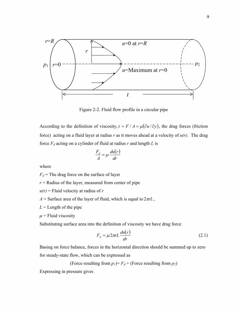
9
Figure 2-2. Fluid flow profile in a circular pipe
According to the definition of viscosity, ( )yuAF ∂∂== // μτ , the drag forces (friction
force) acting on a fluid layer at radius r as it moves ahead at a velocity of u(r). The drag
force Fd acting on a cylinder of fluid at radius r and length L is
( )dr
rduAFd μ=
where
Fd = The drag force on the surface of layer
r = Radius of the layer, measured from center of pipe
u(r) = Fluid velocity at radius of r
A = Surface area of the layer of fluid, which is equal to rLπ2 ,
L = Length of the pipe
μ = Fluid viscosity
Substituting surface area into the definition of viscosity we have drag force
( )dr
rdurLFd πμ2= (2.1)
Basing on force balance, forces in the horizontal direction should be summed up to zero
for steady-state flow, which can be expressed as
(Force resulting from p1)= Fd + (Force resulting from p2)
Expressing in pressure gives
p1 p2
L
u=Maximum at r=0
r
r=0
r=R u=0 at r=R

10
22
21 rpFrp d ππ +=
or
( ) 221 rppFd π−= (2.2)
where
p1 = Inlet pressure,
p2 = Outlet pressure,
πr2 = Cross-section area of the pipe.
Substituting Equation 2.1 into Equation 2.2 yields
( ) ( ) 2212 rpp
drrdurL ππμ −= (2.3)
Separating variables gives
( ) ( )dr
Lrppdr
rLrppdu
μπμπ
2221
221 −
−=−
−= (2.4)
Integrating from the pipe wall to the center and applying boundary conditions
u (r) = u
and
u(r=R)=0
we obtain
( ) ( )⎟⎟⎠
⎞⎜⎜⎝
⎛−
−−=
−−= ∫∫ 2222
222121
0
RrLppdrr
Lppdu
r
R
u
μμ (2.5)
Therefore the velocity of the fluid can be expressed as a function of radius, r.
( ) ( )2221
4rR
Lppu −
−=
μ (2.6)
Using control element concept we can calculate the volumetric flow rate through the
pipe q. Integrating the fluid velocity u over each element of cross-sectional area 2πrdr
(Figure 2-3).

11
Figure 2-3. Cross section view of a circular pipe
Thus we come up with
( ) ( ) ( )L
RpprdrrRLppq
R
μπ
πμ 8
24
421
0
2221 −=−
−= ∫ (2.7)
where
q = Volumetric flow rate,
Equation 2.7 is the famous Poiseville's equation. It should be kept in mind that
Poiseville's equation is applies to incompressible fluids only. For gas, due to its high
compressibility the Poiseville's equation cannot be employed directly. To derive similar
equation for gas flow in the pipe we will combine real gas law and mass conservation.
Now if we know the inlet pressure p1 and average velocity 1u , the pressure p and
velocity u of any point at downstream can be calculated. Mass conservation indicates
that mass flow rate is the same for every horizontal location in the pipe
dtdm
dtdm
=1 (2.8)
where
m = Mass at downstream,
m1 = Mass at inlet,
t = Time,
Control Element
r
dr
R
Pipe Wall
Area of Control Element dA=2πrd
L

12
Expressing in volume and density gives
( ) ( )dtVd
dtVd ρρ
=11 (2.9)
where
V = Volume at downstream,
V1 = Volume at inlet,
ρ = Density at downstream,
ρ1 = Density at inlet,
If we use the average velocity and cross section area to represent the volumetric flow
rate, we have
ρρ AuAu =11 (2.10)
where
u = Average velocity at downstream,
1u = Average velocity at inlet,
A = Cross section area of pipe,
Cancelling out the cross section area yields
ρρ uu =11 (2.11)
Real gas law gives
1111 TnRzVp gas= (2.12)
and
znRTpV = (2.13)
where
T = Temperature at downstream,
T1 = Temperature at inlet,
z = Compressibility at downstream,
z1 = Compressibility at inlet,
n = Mole of gas,
Rgas = Gas constant,
for inlet and downstream, respectively.

13
Multiplying molecular weight to both sides we have
MwTnRzMwVp gas 1111 = (2.14)
and
TMwznRpVMw gas= (2.15)
where
Mw = Molecular weight,
Rearrangement gives
1111
111 ρTRz
VnMwTRz
Mwp gasgas == (2.16)
and
ρTzRVTnMwzR
pMw gasgas == (2.17)
Substituting Equations 2.16 and 2.17 into Equation 2.11 we obtain
TzRpMwu
TRzMwp
ugasgas
=11
11 (2.18)
Since temperature is constant, TT =1 , cancelling out Mw, Rgas, and temperatures yields
zpu
zp
u =1
11 (2.19)
If the pressure drop in the pipe is small comparing with measuring pressure and pressure
drop due to kinetic energy change is negligible, which is the case in this study, Equation
2.7 can be expressed in average velocity
( )L
RppRuAuqμ
ππ
8
4212 −
===
or
( )L
Rppuμ8
221 −
= (2.20)
Expressing in derivative is
μ8
2Rdldpu −= (2.21)

14
Equation 2.19 can be cast to
pzzpuu
1
11= (2.22)
Substituting Equation 2.22 into Equation 2.21 we have
μ8
2
1
11
Rdldp
pzzpu −= (2.23)
Separating variables yields
dlRudp
zppz
21
1
1 8 μ=− (2.24)
Integrating from inlet to outlet we have
∫∫ =−Lp
p
dlRu
dpzp
pz
02
12
1 1
1 8 μ (2.25)
Considering the facts that compressibility factor z and viscosity μ are strong functions of
pressure and the lack of rigorous expressions for these functions, there is no closed-form
expression for integral in Equation 2.25. In case of very low pressure gradient, we
employed zav and μav to denote the average compressibility and viscosity of gas in the
pipe. In this study the pressure difference between inlet and outlet is 0-10 psi, which is
very small comparing with 3000-25000 psig measuring pressure, thus the variation of
viscosity and compressibility with pressure can be neglected. Equation 2.25 is replaced
with
∫∫ =−L
avp
p av
dlR
udp
pzpz
02
12
1 1
1 8 μ (2.26)
or
( ) 212
221
1
1 82 R
Lupp
pzz av
av
μ=− (2.27)
Recasting Equation 2.27 gives
( )( ) 21
21211
1 82 R
Lupppp
pzz av
av
μ=+− (2.28)
or

15
( ) ( )1
2112
211 28 pz
ppzL
Rppuavav
+−=
μ (2.29)
Multiplying by cross section area, 2RA π= we have
( ) ( )1
2114
2121 28 pz
ppzL
RppRuavav
+−=
μπ
π (2.30)
Expressing in volumetric flow rate gives
( ) ( )1
2114
21
28 pzppz
LRppq
avav
+−=
μπ (2.31)
which has an addition term, ( )1
211
2 pzppz
av
+ , accounting for compressible fluid flow.
Equation 2.31 is similar to Poiseville's equation. In case of incompressible fluids,
( )1
211
2 pzppz
av
+ will collapse to 1, and then Equation 2.31 will end up with Poiseville's
equation.
2.1.1 Capillary Viscometers
Transpiration method is the base for capillary viscometer. Capillary viscometer is named
after its key part, a cylindrical capillary tube. It also has another often used name,
Rankine viscometer. In a capillary viscometer, fluid flows through a cylindrical capillary
tube. Figure 2-4 shows a typical capillary viscometer in two positions: (a) is in
horizontal position, and (b) is in vertical position. The measurement principle is the
combination of Poiseville equation and real gas law. Viscosity is determined by
measuring the flow rate of the fluid flowing through the capillary tube and the pressure
differential between both ends of the capillary tube. This measurement method is based
on the laws of physics; therefore, this is called the absolute measurement of viscosity.

16
The principle and structure of the capillary viscometer is simple, but accurate
measurement is the key for success. The inside of the capillary viscometer must be kept
very clean. Also, a thorough drying of the capillary tube is required before each
measurement. Temperature control is essential because the capillary tube is susceptible
to thermal expansion or contraction under the influence of temperature, especially in
lower viscosity ranges. These thermal impacts might introduce errors to the
measurement. In addition, capillary tube is hard to withstand high pressure. A constant
tube diameter and regular geometric shape at HPHT are necessary to obtain good result.
As a result, capillary viscometer is suitable for measurement at low-moderate pressure
and temperature.
The measurement of gas viscosity using capillary viscometer is delineated as follow. 1)
A drop of clean mercury is introduced into a sufficiently narrow cylindrical glass tube
filled with gas, completely fills the cross-section of the tube and forms a practically
perfect internal seal as between the spaces on either side of it; 2) changing the
viscometer from horizontal to any inclination will cause the mercury pellet start to flow
due to the gravity force or the density difference between mercury and gas; 3) mercury
pellet quickly come into equilibrium with the proper difference of gas pressure
established above and below; 4) actually the descending mercury pellet acts as a piston,
forcing the gas through the capillary tube. Any alteration of inclination angle of the
viscometer will change the descending velocity of the mercury pellet.
A typical capillary viscometer is a closed glass vessel consisting of two connected tubes
as shown in Figure 2-5, one is a fine capillary tube and the other is tube with much larger
inner-diameter compared with the former, yet sufficiently narrow for a pellet of mercury
to remain intact in it. The governing equation to calculate gas viscosity from capillary
viscometer is derived as follow (Rankine, 1910).

17
Let V be the volume unoccupied by mercury; the volume of the capillary tube is much
less than V, therefore it is negligible. Let p denote the steady pressure of the gas in the
tube when the viscometer is held horizontally and let Δp be the pressure difference
caused by the mercury pellet when the apparatus is vertical. Let p1 be the pressure and V1
the volume at any time above the mercury, and p2, V2, the corresponding quantities
below the mercury. Then
21 VVV += , and 12 ppp −=Δ (2.32)
Now if we keep the temperature constant, then real gas law gives
2211 VpVppV += (2.33)
Substituting Equation 2.32 into Equation 2.33 we obtain
( ) 212111 pVVpVppVppV Δ+=Δ++= (2.34)
Since 12 VVV −= , Equation 2.34 can be rearranged into
( )11 VVpVppV −Δ+=
or
⎟⎠⎞
⎜⎝⎛Δ+Δ−=
VVpppp 1
1 (2.35)
From Equation 2.35 we can see that the pressure above the mercury increases linearly
with V1, so does the pressure below the mercury, meanwhile the pressure difference
remains constant (caused by the density difference between mercury and gas). Let
dVelementary be an elementary volume of gas emerging from the top end of the capillary.
This will result in an increase of pressure dp1, and also an increase dV1 in Vl. The
relation between these quantities is
1
111 p
dpVdVdVelementary += (2.36)
which can be expressed as
( )1
111 p
dppppp
Vdpp
VdVelementary Δ+−Δ
+Δ
=

18
( )1
11
2p
pppdpp
V Δ+−Δ
= (2.37)
(a) Viscometer in horizontal position (b) Viscometer in vertical position
Figure 2-4. Capillary viscometer in two positions, after Rankine (1910)
Recalling Meyer's (Meyer, 1866) formula for transpiration, and neglecting for the
moment the slipping correction, we can write
( )dtpl
ppRdVelementary1
21
22
4
28μπ −
= (2.38)
( )( )
( )dt
lpRppp
dtlp
RppppdVelementary
1
42
1
41212
162
16
μπ
μπ
Δ−Δ=
−+=
(2.39)
where
p2 =p1+Δp
Δp = Pressure difference (Reading from gauge) measured in cms. of mercury at 0oC

19
μ = Air viscosity
R = Radius of capillary tube
L = Length of the capillary tube
If we assume that p1 and p2 change sufficiently slowly for the steady state to be set up
without appreciable lag; let KlR =μπ 8/4 , and substituting for p2 in Equation 2.39, we
obtain
( )dt
ppppKdVelementary
1
2
22 Δ−
Δ= (2.40)
By comparing right hand side of Equations 2.37 and 2.40 we note that they are equal.
( ) ( )dt
ppppK
ppppdp
pV
1
2
1
11 2
22 Δ−Δ=
Δ+−Δ
(2.41)
Let ppx Δ+= 12 and 12dpdx = , Equation 2.41 can be written as
( ) pxdtKdxpxp
VΔ=−
Δ (2.42)
Integration of Equation 2.42 gives
( ) pdtKxpxp
V xx Δ=−
Δ21log (2.43)
Recalling ⎟⎠⎞
⎜⎝⎛Δ+Δ−=
VVpppp 1
1 from Equation 2.35, then
⎟⎠⎞
⎜⎝⎛ −Δ−=Δ+⎥
⎦
⎤⎢⎣
⎡⎟⎠⎞
⎜⎝⎛Δ+Δ−=
Vvppp
Vvpppx 11 2122 (2.44)
Suppose that t is the time taken for the upper volume to increase from V1 to V1’, the
following is the equation giving the air viscosity.
( )ptK
VVpp
VVpp
pV
VVpp
VΔ=
⎪⎪
⎭
⎪⎪
⎬
⎫
⎪⎪
⎩
⎪⎪
⎨
⎧
⎥⎥⎥⎥⎥
⎦
⎤
⎢⎢⎢⎢⎢
⎣
⎡
⎟⎠⎞
⎜⎝⎛ −Δ−
⎟⎟⎠
⎞⎜⎜⎝
⎛−Δ−
−−Δ
Δ 1
'1
1'
1
212
212log
2 (2.45)
By substituting KlR =μπ 8/4 into Equation 2.45 we have

20
( )lptR
VVpp
VVpp
ppVVV
μπ
8212
212log2
4
1
'1
1'
1Δ
=
⎥⎥⎥⎥⎥
⎦
⎤
⎢⎢⎢⎢⎢
⎣
⎡
⎟⎠⎞
⎜⎝⎛ −Δ−
⎟⎟⎠
⎞⎜⎜⎝
⎛−Δ−
Δ−− (2.46)
It should be noted that the capillary attraction in the wider limb makes the value of Δp
not proportional to the length of the mercury pellet. If the pellet was undeformed by the
downward movement, capillarity would produce no resultant effect, taking account of
the symmetry of the ends. Actually, the upper surface is less curved than the lower one
during the motion. This results in a diminution of the effective driving pressure.
A classic capillary viscometer used by Rankine (1923) to measure the viscosities of
neon, xenon, and krypton is illustrated as Figure 2-5. Detail geometry of the apparatus
can be obtained from Rankine (1910).
Figure 2-5. A classic capillary viscometer, after Rankine (1910)

21
2.1.2 Falling (or Rolling) Ball Viscometers
From its name we know that the falling (or rolling) ball viscometer measures viscosity
by dropping a column- or sphere-shaped rigid body with known dimensions and density
into a sample and measuring the time taken for it to fall a specific distance (Figure 2-6).
Another type of device measures traveling time when horizontally transporting a rigid
body, such as a piston or a needle, in a sample fluid at a constant speed by the force
applied by the electromagnetic field. All falling-body viscometers measure fluid
viscosity basing on Stokes' law.
Figure 2-6. Cross section of falling cylinder viscometer body and ancillary components, after Chan and Jckson (1985)

22
Unlike the vibrating or rotational viscometers, the falling-ball viscometers shown Figure
2-6 cannot continuously measure viscosity. It is also impossible to continuously output
digital signals of viscosity coefficient or to control data. In falling ball viscometer the
fluid is stationary in a vertical glass tube. A sphere of known size and density is allowed
to descend through the fluid. The time for the ball to fall from start point to the end point
on the tube can be recorded and the length it travels can be measured. Electronic sensing
can be used for timing. At the end of the tube there are two marks, the time for the ball
passing these two marks are recorded so that the average velocity of the ball is calculated
assuming the distance between these two marks is close enough. Knowing the terminal
velocity, the size and density of the sphere, and the density of the liquid, Stokes' Law can
be used to calculate the viscosity.
Besides the use of a sphere in falling ball viscometers, both cylinders and needles have
been used by various researchers to measure the viscosity. Instruments are also available
commercially using these types of geometry. Therefore, commonly used falling ball
viscometer includes falling ball, falling cylinder, and falling needle viscometers. Figure
2-7 is the illustration of a falling ball viscometer. Typical falling cylinder viscometer can
be referred to Figure 2-6 mentioned above. An example of falling needle viscometer can
be seen in Figure 2-8.

23
Figure 2-7. Cross section of a falling ball viscometer body, after Florida Atlantic
University (2005)
There are some drawbacks when the viscosity is measure by the ball viscometer, these
include that the motion of the ball during its descent in the viscometer tube exhibits
random slip and spin (Herbert and Stoke, 1886). If we use a cylinder instead of a ball,
the problem can be overcome easily. First, a cylinder equipped with stabilizing
projections, shows little if any tendency toward dissipating energy in this fashion. Thus
the error in measuring experimental fall times is reduced. Second, when ball viscometers
are used for measuring low viscosities, the ball diameter must be nearly equal to the tube
diameter, making the instrument extremely sensitive to the effects of nonuniform
construction, poor reproducibility results. The cylinder however may be easily oriented
in a consistent fashion so that any effect of nonuniform construction is constant (Dabir et
al., 2007).

24
Figure 2-8. Cross section of a falling needle viscometer body, after Park (1994)
Rolling ball viscometers employ the same measuring method as falling ball viscometer
except that the falling trajectory is slant instead of vertical. A classic rolling ball
viscometer is shown in Figure 2-9.

25
Figure 2-9. Rolling ball viscometer, after Tomida et al. (2005)
2.1.3 Vibrating viscometers
Vibrating viscometers can be dated back to the 1950s Bendix instrument, which is of a
class that operates by measuring the damping of an oscillating electromechanical
resonator immersed in a fluid whose viscosity is to be determined. The resonator
generally oscillates in torsion or transversely as a cantilever beam or tuning fork. They
are rugged industrial systems used to measure viscosity in many fields. The principle of
vibrating viscometer is that it measures the damping of an oscillating electromechanical
resonator immersed in the test liquid. The resonator may be a cantilever beam,
oscillating sphere or tuning fork which oscillates in torsion or transversely in the fluid.
The resonator's damping is measured by several methods:
1) Measuring the power input necessary to keep the oscillator vibrating at constant
amplitude. The higher the viscosity, the more power is needed to maintain the
amplitude of oscillation.
2) Measuring the decay time of the oscillation once the excitation is switched off.
The higher the viscosity, the faster the signal decays.

26
3) Measuring the frequency of the resonator as a function of phase angle between
excitation and response waveforms. The higher the viscosity, the larger the
frequency changes for a given phase change.
The designation of vibrating viscometer usually uses three technologies. There are
tuning fork, oscillating sphere, and vibrating rod (or wire) technologies. Each of these
technologies is described as follow.
Tuning fork technology-vibrational viscometers designed based on tuning fork
technology measure the viscosity by determining the bandwidth and frequency of the
vibrating fork resonance; the bandwidth giving the viscosity measurement whilst the
frequency giving the fluid density (Figure 2-10). A temperature sensor can be easily
accommodated in the instrument for temperature measurement. In addition, other
parameters such as viscosity gravity gradients and ignition indices for fuel oils can be
calculated.
Figure 2-10. Vibrational viscometer employed tuning fork technology, after Paul N.
Gardner Co. (2010)

27
Oscillating sphere technology - in this method a sphere oscillates (Figure 2-11) about its
polar axis with precisely controlled amplitude (Steffe, 1992). The viscosity is calculated
from the power required to maintain this predetermined amplitude of oscillation. While
it is very simple in design, the oscillating sphere viscometer provides viscosity that is
density dependent. Therefore, density of the test fluid should be determined
independently if kinematic viscosity is required for process control. The principle of
oscillating sphere viscometer had been studied by Stokes (1868) many years ago.
Figure 2-11. An oscillating sphere system for creating controlled amplitude in liquid,
after Steffe (1992)

28
Vibrating rod (or wire) technology - in the viscometer the active part of the sensor is a
vibrating rod (or wire). The vibration amplitude varies according to the viscosity of the
fluid in which the rod is immersed (Figure 2-12).
Figure 2-12. Vibrating rod system for measuring dynamic viscosity, after Steffe (1992)
Vibrating viscometers are best suited for many requirements in viscosity measurement.
The important features of vibrating viscometers are small sample volume requirement,
high sensitivity, ease of operation, continuous readings, wide range, optional internal
reference, flow through of the test fluids and consequent easy clean out and prospect of
construction with easily available materials. Contrasted to rotational viscometers, which
require more maintenance and frequent calibration after intensive use, vibrating
viscometers has no moving parts, no weak parts and the sensitive part is very small.
Actually even the very basic or acid fluid can be measured by adding a special coating or
by changing the material of the sensor. Currently, many industries around the world
consider these viscometers as the most efficient system to measure viscosity of any fluid.

29
2.2 Gas Viscosity Experimental Data
Common approach to estimate gas viscosity comprises direct experimental measurement
and gas viscosity correlations. Direct measurement provides reliable and confident result
so with the cost of high expense and time consuming and cost expensive. Furthermore,
quantity of fluid sample and availability of appropriate measuring instrument that can
handle experiment at reservoir condition limit its application. Given the aforementioned
disadvantages most PVT lab reports provided gas viscosity estimated from correlations.
Although gas viscosity correlation provides a simple and low cost method to predict gas
viscosity, accuracy of calculated viscosity is depended on the database it based on. A
good gas viscosity correlation needs accurate lab data as its solid base. We cannot
evaluate the correlation before we know what kind of lab data is used. One thing for sure
is that a correlation cannot guarantee its validity outside of the thermodynamic conditions
of lab data. Thus, it is necessary to understand the limitation of available gas viscosities
database. In this study a review of available pure nitrogen, methane, and natural gas
viscosity is crucial to make our project sense considering high methane concentration in
most HPHT gas reservoirs and high nonhydrocarbon concentration such as nitrogen in
some HPHT gas reservoirs.
Earhart (1916) determined 10 natural gases viscosities using a capillary viscometer. Yen
(1919) measured nitrogen viscosity at temperature of 23 oC and pressures of 14.7 psia
using a capillary viscometer. Boyd (1930) applied the transpiration method, or same
principle as capillary viscometer, on measuring nitrogen viscosity at temperatures of 30,
50, and 70 oC and pressures from 73 to 178.8 atms. Trautz and Zink (1930) measured
methane and nitrogen viscosities at temperatures from 23 to 499 oC. Michels and Gibson
(1931) designed an apparatus basing on capillary principle to measure nitrogen viscosity
at temperatures of 25, 50, and 75 oC and pressures from 15.37 to 965.7 atms. Berwald
and Johnson (1933) measured 25 natural gases viscosities at temperature of 60 oF and
pressure of 29.4 psia with a capillary viscometer. Rudenko and Schubnikow (1934)
measured nitrogen viscosities at temperature from 63 to 77 oK and pressure less than 8

30
psia with a capillary viscometer. Adzumi (1937) measured methane, ethane, propane,
CH4-C2H2, C2H2-C3H6, and C3H6-C3H8 mixtures viscosities at temperature from 0 to
100 oC and pressure of 14.7 psia with a capillary viscometer. Sage and Lacey (1938)
measured methane and 2 natural gases viscosity at temperatures of 100, 160, and 220 oF
and pressures up to 2600 psi. Johnston and McCloskey (1940) measured methane and
nitrogen viscosity at temperatures from 90 to 200 oK and pressures up to 14.7 psia using
an oscillating-disk viscometer. Smith and Brown (1943) measured pure ethane and
propane viscosities at temperatures from 15 to 200 oC and pressures from 100 to 5000
psi utilizing a rolling-ball viscometer. They also developed a viscosity correlation basing
on available data. Bicher and Katz (1943) measured pure methane and methane-propane
mixture viscosities utilizing a rolling-ball inclined-tube viscometer. They ran
experiments at temperatures of 77, 167, 257, 347, and 437 oF and pressures from 14.7 to
5000 psia. Comings et al. (Comings and Egly, 1940; Coming et al., 1944) used two
Rankine viscometers (capillary viscometer) constructed of Pyrex glass to measure
methane and natural gas viscosities at temperatures of 30, 50, 70, and 95 oC and
pressures from 1 to 171 atms. Similar to Comings’s study, Van Itterbeek et al. (1947)
measured nitrogen viscosity at temperatures from -312 to 64 oF and low to ordinary
pressures with an oscillating disc viscometer. Carr (1952) and Stewart (1952) used two
Rankine viscometers (capillary viscometer) constructed of Pyrex glass to measure
methane and three natural gas viscosities at temperatures from 70 to 200 oF and
pressures from 14.7 to 10000 psia. Iwasaki (1954) measured pure nitrogen and nitrogen-
hydrogen mixture viscosities utilizing an oscillating disc viscometer at temperatures of
25, 100, and 150 oC and pressures up to 200 atms. Lambert et al. (1955) measured
methane and ethane viscosities an oscillating viscometer at temperatures from 35 to 78 oC and low pressures. Ross and Brown (1957) used a capillary tube viscometer to
measure pure nitrogen and methane viscosities at temperatures of 25, 0, -25, and -50 oC
and pressures from 500 to 10000 psig. Ellis and Raw (1958) measured nitrogen viscosity
at temperatures from 700 to 1000 oC and low pressures through a capillary tube
viscometer. Baron et al. (1959) used Rankine viscometer (capillary viscometer) to

31
measure pure nitrogen and methane viscosities at temperatures of 125, 175, 225, and 275 oF and pressures from 100 to 8000 psig. To solve the problem of grass capillary
viscometer broken at high pressure, he balanced the pressures between inside and
outside of tube by charging the annulus around the tube. Kestin and Leidenfrost (1959)
constructed an oscillating-disk viscometer to measure pure nitrogen viscosities at
temperatures from 19 to 25 oC and pressures from 0.139 to 62.7 atms. Swift et al. (1959)
measured methane viscosity at temperatures from -83 to -150 oC and pressures from 350
to 710 psia with a falling-body viscometer. Golubev (1959) used the capillary tube
viscometer to measure pure nitrogen and methane viscosities at condition of
temperatures range from –58.12 to 1292 ºF and pressures range from 14.7 to 14700 psia.
Golubev data shows a significant difference compared data from the other available
database. Swift et al. (1960) extended his measurement on methane viscosity at
temperatures from -82 to -140 oC and pressures from 85 to 675 psia with a falling-
cylinder viscometer. Flynn et al. (1963) developed a capillary viscometer to measure
nitrogen viscosity at temperatures of -78, -50, -25, 25, and 100 oC and pressures from
6.77 to 176 atms. Barua et al. (1964) measured methane viscosity at temperatures from -
50 to 150 oC and pressures up to 200 atms using a capillary viscometer. Carmichael et al.
(1965) measured methane viscosity at temperatures of 40, 100, 220, 340, and 400 oF and
pressures from 14.7 to 5000 psia using a rotating-cylinder type viscometer. Lee (1965)
presented viscosity values of pure methane basing on work done by Mario Gonzalez.
Data were acquired at temperature from 100 to 340 oF and pressure from 200 to 8000
psia. Recommended methane viscosity values are presented in Table 2-1. Lee claimed
that viscosity values corresponding to the region of this investigation are accurate within
±5% percent. Lee also collected pure hydrocarbons such as ethane, propane, n-butane, n-
pentane, and n-decane and gas mixtures (methane-propane, methane-butane, and
methane-decane) viscosities in order to derive gas viscosity correlation. He considered
the following mole percentage: 10, 20, 30, 40, 50, 60, 70, 80, and 90 percent in binary
mixtures. Giddings et al. (1965) developed a versatile absolute capillary-tube viscometer
to measure methane viscosity at temperatures from 40 to 280 oF and pressures from 100

32
to 8000 psia. Wilson (1965) constructed a rolling ball viscometer to measure 10 natural
gases viscosity at temperatures from 77 to 400 oF and pressures from 1000 to 10000 psia.
Dipippo et al. (1966) constructed an oscillating disc viscometer to measure nitrogen
viscosity at temperatures from 75 to 410 oF and pressures from 5.7 to 25 psia. Lee and
Gonzalez et al. (Gonzalez et al., 1966; Gonzalez et al.,1970) measured the viscosities of
eight natural gases using a capillary-tube viscometer to honor the true reservoirs, for all
of the samples, the range of temperature is 100 to 340 ºF and the range of pressure is
from 14.7 to 8000 psia. Gonzalez et al. (1966) published his methane viscosity data
covered temperatures from 100 to 340 ºF and pressures from 200 to 8000 psia. Huang et
al. (1966) measured methane viscosities at temperatures from -170 to 0 ºC and pressure
up to 5000 psia with a falling cylinder type viscometer. Van Itterbeek et al. (1966)
provided nitrogen viscosities measured by a oscillating disk viscometer at temperatures
of 70, 77.3, 83.9 and 90.1 ºK and pressures from 0.5 to 98 atms. Boon et al. (1967)
provided methane and nitrogen viscosities measured by a capillary viscometer at
temperatures from 91 to 114 ºK and the corresponding saturated vapor pressures. Kestin
and Yata (1968) measured pure methane, nitrogen, and H2-N2, CH4-CO2, CH4-C4H10
binary mixtures viscosities using an oscillating-disk viscometer at temperatures 20 and
30 ºC and pressures from 1 to 25 atms. Grevendonk et al. (1970) measured liquid
nitrogen viscosity using a torsionally vibrating piezoelectric crystal viscometer at
temperatures from 66 to 124 ºK and pressures from vapor pressure to 196 x 105 N/m2.
Helleman et al. (Helleman et al., 1970; Helleman et, al. 1973) measured methane
viscosities at temperatures from 96 to 187 ºK and pressures up to 100 atms and nitrogen
viscosities at temperatures from 77 to 203 ºF and pressures of 14.7 psia using an
oscillating-disk viscometer. Diehl et al. (1970) used Geopal viscometer (capillary tube
viscometer) to determine the pure hydrocarbon and nitrogen gas viscosities. For all of
the samples, the range of temperature is 32 to 302 ºF and the range of pressure is from
14.7 to 7350 psia. Latto and Saunders (1972) measured nitrogen viscosity at
temperatures from 90 to 400 ºK and pressures from 1 to 150 atms using a capillary
viscometer. Stephan and Lucas (1979) collected a large database of gas viscosities from

33
several investigators with different methods including torsional crystal, oscillating disk,
rolling ball, rotating cylinder, capillary tube, and falling ball. The data includes gases
such as pure hydrocarbons (methane to n-decane), nitrogen, and carbon dioxide. The
range of temperatures and pressures differs from one component to another. In general
the temperatures range is from 212 to 1832 ºF and the pressures range is from 14.7 to
10290 psia. Diller (1980) measured the viscosity of compressed gases and liquid
methane at temperatures between 100 and 300 ºK and pressures up to 4350 psia with a
torsionally oscillating quartz crystal viscometer. As a extension of his work in 1980,
Diller (1983) used same viscometer to measure the viscosity of compressed gases and
liquid nitrogen at temperatures between 90 and 300 ºK and pressures up to 4350 psia.
Hongo et al. (1988) used Maxwell type oscillating-disc viscometer to measure the
viscosity of methane and methane-chlorodifluoromethane mixtures in the temperature
range from 298.15 to 373.15 oK and at pressures up to 5MP. Van Der Gulik et al. (1988)
used vibrating wire viscometer to measure the viscosity of methane at 25 ºC and
pressures from 1 to 10,000 bar. Vogel et al. (1999) used a vibrating wire viscometer to
measure the viscosity of methane at temperature of 260, 280, 300, 320, 340, and 360 ºK
and pressures up to 20 MPa. Assael et al. (2001) employed a vibrating wire viscometer
to measure the viscosity of methane at the temperature range from 313 to 455 oK at a
pressure close to atmospheric and in the temperature range from 240 to 353 oK at
pressures up to 15 MPa. Schley et al. (2004) used a vibrating-wire viscometer to
measure methane viscosity at temperatures of 260, 280, 300, 320, 340, and 360 K and at
pressures up to 29 MPa. Seibt et al. (2006) measured nitrogen viscosity with a vibrating-
wire viscometer. The measurements were performed along the six isotherms of 298.15,
323.15, 348.15, 373.15, 398.15, and 423.15 oK and at pressures up to a maximum of 35
MPa. Tables 2-1 to 2-4 show experimental data of methane viscosity from some
investigators. Table 2-5 depicts experimental data of nitrogen viscosity from some
investigators.

34
Table 2-1. Methane viscosity collected by Lee (1965)
Pressure Temperature (oF) (psia) 100 160 220 280 340 400 460 14.70 0.01140 0.01250 0.01340 0.01440 0.01530 0.01660 0.01750 100.00 0.01190 0.01300 0.01400 0.01500 0.01600 0.01700 0.01790 200.00 0.01200 0.01300 0.01410 0.01510 0.01610 0.01710 0.01800 300.00 0.01210 0.01310 0.01410 0.01510 0.01620 0.01720 0.01800 400.00 0.01220 0.01320 0.01420 0.01520 0.01620 0.01730 0.01810 500.00 0.01240 0.01330 0.01430 0.01530 0.01630 0.01730 0.01820 600.00 0.01250 0.01350 0.01440 0.01540 0.01640 0.01740 0.01830 800.00 0.01280 0.01370 0.01460 0.01550 0.01650 0.01760 0.01840 1000.00 0.01320 0.01400 0.01480 0.01570 0.01670 0.01780 0.01860 1250.00 0.01370 0.01450 0.01520 0.01600 0.01700 0.01800 0.01880 1500.00 0.01440 0.01490 0.01560 0.01630 0.01720 0.01830 0.01910 1750.00 0.01520 0.01540 0.01600 0.01680 0.01750 0.01850 0.01930 2000.00 0.01600 0.01600 0.01640 0.01700 0.01780 0.01860 0.01950 2500.00 0.01770 0.01720 0.01740 0.01780 0.01850 0.01940 0.02010 3000.00 0.01950 0.01860 0.01860 0.01870 0.01930 0.02010 0.02070 3500.00 0.02120 0.02020 0.01970 0.01970 0.02010 0.02070 0.02130 4000.00 0.02310 0.02170 0.02090 0.02060 0.02090 0.02140 0.02190 4500.00 0.02490 0.02320 0.02200 0.02170 0.02180 0.02220 0.02250 5000.00 0.02660 0.02460 0.02330 0.02280 0.02260 0.02300 0.02320 6000.00 0.02990 0.02740 0.02570 0.02500 0.02440 0.02450 0.02460 7000.00 0.03280 0.02990 0.02810 0.02710 0.02620 0.02610 0.02600 8000.00 0.03550 0.03230 0.03000 0.02910 0.02810 0.02750 0.02730 9000.00 0.03800 0.03450 0.03220 0.03100 0.03000 0.02910 0.02860 10000.00 0.04060 0.03660 0.03420 0.03300 0.03180 0.03050 0.03000 Note: viscosity in cp

35
Table 2-2. Methane viscosity by Diehl et al. (1970)
Pressure Temperature (oF) (psia) 86 104 122 140 158 176 194
14.70 0.01116 0.01150 0.01183 0.01216 0.01248 0.01279 0.01310220.50 0.01140 0.01170 0.01205 0.01235 0.01270 0.01300 0.01330367.50 0.01155 0.01190 0.01220 0.01255 0.01285 0.01320 0.01350735.00 0.01210 0.01240 0.01270 0.01300 0.01335 0.01365 0.01400
1102.50 0.01290 0.01315 0.01340 0.01365 0.01395 0.01425 0.014551470.00 0.01390 0.01410 0.01430 0.01450 0.01470 0.01490 0.015151837.50 0.01510 0.01520 0.01530 0.01545 0.01560 0.01575 0.015902205.00 0.01640 0.01640 0.01645 0.01650 0.01655 0.01665 0.016752940.00 0.01905 0.01895 0.01885 0.01875 0.01870 0.01865 0.018603675.00 0.02175 0.02150 0.02125 0.02105 0.02085 0.02070 0.020554410.00 0.02410 0.02380 0.02350 0.02320 0.02290 0.02265 0.022405145.00 0.02650 0.02610 0.02570 0.02530 0.02490 0.02455 0.024255880.00 0.02880 0.02830 0.02780 0.02730 0.02685 0.02640 0.026006615.00 0.03105 0.03045 0.02990 0.02930 0.02875 0.02825 0.027757350.00 0.03320 0.03250 0.03190 0.03125 0.03060 0.03000 0.02945Note: viscosity in cp
Table 2-2. Continued
Pressure Temperature (oF) (psia) 212 230 248 266 280 302
14.70 0.01341 0.01371 0.01400 0.01430 0.01459 0.01488 220.50 0.01360 0.01395 0.01425 0.01455 0.01485 0.01515 367.50 0.01380 0.01410 0.01440 0.01470 0.01500 0.01530 735.00 0.01430 0.01460 0.01490 0.01515 0.01545 0.01575
1102.50 0.01480 0.01505 0.01535 0.01560 0.01585 0.01610 1470.00 0.01540 0.01565 0.01590 0.01615 0.01635 0.01655 1837.50 0.01610 0.01630 0.01650 0.01670 0.01690 0.01710 2205.00 0.01685 0.01700 0.01715 0.01730 0.01750 0.01770 2940.00 0.01860 0.01865 0.01870 0.01880 0.01890 0.01900 3675.00 0.02045 0.02040 0.02035 0.02030 0.02025 0.02025 4410.00 0.02220 0.02205 0.02190 0.02180 0.02170 0.02160 5145.00 0.02395 0.02370 0.02350 0.02330 0.02315 0.02300 5880.00 0.02565 0.02535 0.02505 0.02475 0.02450 0.02430 6615.00 0.02730 0.02690 0.02655 0.02620 0.02590 0.02565 7350.00 0.02890 0.02845 0.02805 0.02765 0.02730 0.02700 Note: viscosity in cp
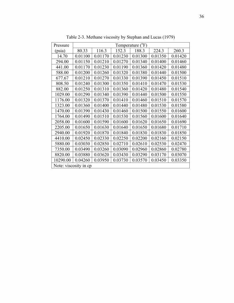
36
Table 2-3. Methane viscosity by Stephan and Lucas (1979)
Pressure Temperature (oF) (psia) 80.33 116.3 152.3 188.3 224.3 260.3
14.70 0.01100 0.01170 0.01230 0.01300 0.01350 0.01420 294.00 0.01150 0.01210 0.01270 0.01340 0.01400 0.01460 441.00 0.01170 0.01230 0.01190 0.01360 0.01420 0.01480 588.00 0.01200 0.01260 0.01320 0.01380 0.01440 0.01500 677.67 0.01210 0.01270 0.01330 0.01390 0.01450 0.01510 808.50 0.01240 0.01300 0.01350 0.01410 0.01470 0.01530 882.00 0.01250 0.01310 0.01360 0.01420 0.01480 0.01540 1029.00 0.01290 0.01340 0.01390 0.01440 0.01500 0.01550 1176.00 0.01320 0.01370 0.01410 0.01460 0.01510 0.01570 1323.00 0.01360 0.01400 0.01440 0.01480 0.01530 0.01580 1470.00 0.01390 0.01430 0.01460 0.01500 0.01550 0.01600 1764.00 0.01490 0.01510 0.01530 0.01560 0.01600 0.01640 2058.00 0.01600 0.01590 0.01600 0.01620 0.01650 0.01690 2205.00 0.01650 0.01630 0.01640 0.01650 0.01680 0.01710 2940.00 0.01920 0.01870 0.01840 0.01830 0.01830 0.01850 4410.00 0.02450 0.02330 0.02250 0.02200 0.02160 0.02150 5880.00 0.03030 0.02850 0.02710 0.02610 0.02530 0.02470 7350.00 0.03490 0.03260 0.03090 0.02960 0.02860 0.02780 8820.00 0.03880 0.03620 0.03430 0.03290 0.03170 0.03070 10290.00 0.04260 0.03950 0.03730 0.03570 0.03450 0.03350 Note: viscosity in cp

37
Table 2-3. Continued
Pressure Temperature (oF) (psia) 296.3 332.3 368.3 404.3 440.3 476.3
14.70 0.01470 0.01540 0.01600 0.01660 0.01720 0.01770 294.00 0.01530 0.01600 0.01660 0.01720 0.01780 0.01840 441.00 0.01540 0.01610 0.01670 0.01730 0.01790 0.01850 588.00 0.01560 0.01620 0.01680 0.01740 0.01800 0.01860 677.67 0.01570 0.01630 0.01690 0.01750 0.01810 0.01870 808.50 0.01580 0.01640 0.01700 0.01760 0.01820 0.01880 882.00 0.01590 0.01640 0.01700 0.01760 0.01820 0.01880 1029.00 0.01600 0.01660 0.01720 0.01780 0.01830 0.01890 1176.00 0.01620 0.01670 0.01730 0.01790 0.01850 0.01910 1323.00 0.01630 0.01690 0.01750 0.01810 0.01860 0.01920 1470.00 0.01650 0.01700 0.01760 0.01820 0.01870 0.01930 1764.00 0.01690 0.01740 0.01800 0.01850 0.01900 0.01960 2058.00 0.01730 0.01780 0.01830 0.01880 0.01930 0.01990 2205.00 0.01750 0.01800 0.01850 0.01900 0.01950 0.02010 2940.00 0.01870 0.01900 0.01950 0.01990 0.02040 0.02090 4410.00 0.02140 0.02150 0.02170 0.02190 0.02220 0.02250 5880.00 0.02440 0.02410 0.02410 0.02410 0.02430 0.02450 7350.00 0.02730 0.02680 0.02660 0.02640 0.02630 0.02630 8820.00 0.03000 0.02940 0.02890 0.02860 0.02830 0.02820 10290.00 0.03260 0.03180 0.03130 0.03070 0.03030 0.03000 Note: viscosity in cp

38
Table 2-4. Methane viscosity by Golubev (1959)
Pressure Temperature (oF) (psia) 77 122 167 212 302 392 482 14.70 0.01108 0.01182 0.01260 0.01331 0.01471 0.01603 0.01725146.96 0.01120 0.01193 0.01270 0.01340 0.01477 0.01611 0.01728293.92 0.01137 0.01210 0.01280 0.01350 0.01483 0.01617 0.01733587.84 0.01180 0.01247 0.01312 0.01377 0.01512 0.01634 0.01745881.76 0.01237 0.01295 0.01350 0.01416 0.01530 0.01653 0.017651175.68 0.01310 0.01352 0.01392 0.01452 0.01556 0.01675 0.017851469.59 0.01395 0.01417 0.01445 0.01497 0.01580 0.01700 0.018092204.39 0.01652 0.01610 0.01600 0.01627 0.01685 0.01775 0.018722939.19 0.01930 0.01830 0.01787 0.01787 0.01807 0.01867 0.019473673.99 0.02187 0.02062 0.02002 0.01965 0.01942 0.01975 0.020304408.78 0.02455 0.02300 0.02205 0.02142 0.02085 0.02075 0.021205143.58 0.02705 0.02530 0.02401 0.02320 0.02230 0.02182 0.022055878.38 0.02942 0.02745 0.02593 0.02486 0.02370 0.02290 0.022957347.97 0.03365 0.03145 0.02955 0.02815 0.02635 0.02500 0.024708817.57 0.03740 0.03485 0.03277 0.03120 0.02887 0.02705 0.0264510287.16 0.04087 0.03820 0.03545 0.03395 0.03130 0.02910 0.0282011756.76 0.04410 0.04095 0.03855 0.03655 0.03367 0.03107 0.02995Note: viscosity in cp

39
Table 2-5. Nitrogen viscosity collected by Stephan and Lucas (1979)
Temperature Pressure (psi) oF 14.504 145 290 435 580 725
-343 0.2633 0.2677 0.2728 0.2777 0.2826 0.2876 -334 0.2113 0.2154 0.2197 0.2244 0.229 0.2336 -325 0.1677 0.1713 0.1753 0.1793 0.1832 0.1875 -316 0.00552 0.1366 0.14 0.1433 0.1467 0.1501 -307 0.00586 0.1111 0.1136 0.1164 0.1192 0.1219 -298 0.0062 0.09326 0.09528 0.09737 0.09951 0.1018 -289 0.00654 0.08093 0.08266 0.08429 0.08602 0.08777 -280 0.00688 0.0713 0.07297 0.07459 0.07616 0.07772 -271 0.00722 0.00783 0.06397 0.06584 0.0676 0.06929 -262 0.00756 0.00811 0.05517 0.05728 0.05925 0.06112 -253 0.00789 0.0084 0.04626 0.04902 0.0514 0.05354 -244 0.00821 0.00868 0.00953 0.03974 0.04335 0.04612 -235 0.00852 0.00896 0.00968 0.01155 0.03369 0.0381 -226 0.00883 0.00925 0.00988 0.01107 0.01805 0.02945 -217 0.00914 0.00954 0.0101 0.01103 0.01314 0.01998 -208 0.00945 0.00983 0.01028 0.01112 0.0125 0.01551 -190 0.01006 0.01041 0.01085 0.01145 0.01232 0.01365 -172 0.01066 0.01098 0.01138 0.01186 0.01252 0.0134 -154 0.01124 0.01154 0.01189 0.01232 0.01286 0.01353 -136 0.01181 0.01209 0.01241 0.01279 0.01325 0.0138 -118 0.01237 0.01263 0.01293 0.01327 0.01367 0.01415 -100 0.01292 0.01316 0.01344 0.01376 0.01411 0.01452 -82 0.01346 0.01369 0.01395 0.01424 0.01456 0.01493 -64 0.01399 0.01421 0.01445 0.01472 0.01502 0.01535 -46 0.0145 0.01471 0.01494 0.01519 0.01546 0.01577 -28 0.015 0.0152 0.01542 0.01566 0.01591 0.01619 -10 0.01549 0.01568 0.01589 0.01612 0.01635 0.01661
Note: viscosity in cp

40
Table 2-5. Continued
Temperature Pressure (psi) oF 14.504 145 290 435 580 725 8 0.01597 0.01615 0.01635 0.01657 0.01679 0.01703 26 0.01644 0.01662 0.0168 0.01701 0.01722 0.01745 44 0.01691 0.01708 0.01726 0.01745 0.01765 0.01787 62 0.01737 0.01753 0.01771 0.01789 0.01808 0.01829 80 0.01782 0.01797 0.01815 0.01832 0.0185 0.0187 98 0.01826 0.01841 0.01858 0.01874 0.01892 0.0191 116 0.0187 0.01885 0.019 0.01916 0.01934 0.01951 134 0.01913 0.01928 0.01942 0.01958 0.01975 0.01991 152 0.01956 0.01971 0.01985 0.02 0.02015 0.02032 170 0.02 0.02014 0.02028 0.02042 0.02056 0.02073 260 0.02204 0.02216 0.02228 0.0224 0.02253 0.02267 350 0.02396 0.02406 0.02417 0.02428 0.02439 0.02451 440 0.02577 0.02586 0.02596 0.02606 0.02615 0.02626 530 0.02747 0.02756 0.02764 0.02774 0.02782 0.02791 620 0.02908 0.02916 0.02924 0.02932 0.0294 0.02948 710 0.03062 0.03069 0.03077 0.03084 0.03091 0.03099 800 0.0321 0.03217 0.03224 0.0323 0.03237 0.03244 980 0.03491 0.03497 0.03503 0.03509 0.03514 0.03521 1160 0.03753 0.03758 0.03763 0.03769 0.03774 0.03779 1340 0.03999 0.04004 0.04008 0.04013 0.04018 0.04023 1520 0.04232 0.04236 0.0424 0.04245 0.04249 0.04253 1700 0.04453 0.04457 0.04461 0.04465 0.04469 0.04473 1880 0.04662 0.04666 0.04669 0.04673 0.04677 0.0468
Note: viscosity in cp

41
Table 2-5. Continued
Temperature Pressure (psi) oF 870 1015 1160 1305 1450 1813
-343 0.2927 0.2978 0.3027 - - - -334 0.2383 0.2429 0.2475 0.2523 0.2568 0.2687 -325 0.1914 0.1957 0.1998 0.2041 0.2084 0.2191 -316 0.1537 0.1573 0.1609 0.1645 0.1682 0.1777 -307 0.1248 0.1278 0.1308 0.1338 0.1369 0.1448 -298 0.104 0.1063 0.1087 0.1111 0.1136 0.12 -289 0.08951 0.09135 0.09319 0.09507 0.097 0.102 -280 0.07922 0.08076 0.08229 0.08386 0.08542 0.08949 -271 0.07089 0.07242 0.07392 0.07539 0.07681 0.08034 -262 0.06294 0.06469 0.06636 0.06794 0.06948 0.07308 -253 0.05553 0.05737 0.0591 0.06078 0.06243 0.06636 -244 0.04849 0.05041 0.05255 0.05437 0.05608 0.06005 -235 0.04135 0.04407 0.04633 0.04836 0.05023 0.05445 -226 0.03424 0.03763 0.04033 0.0427 0.04479 0.04931 -217 0.02686 0.03131 0.03462 0.0373 0.0397 0.04427 -208 0.02068 0.02544 0.02923 0.03229 0.03487 0.04012 -190 0.0157 0.01847 0.02147 0.02434 0.02696 0.03248 -172 0.0146 0.01614 0.018 0.02004 0.02211 0.02698 -154 0.01437 0.01542 0.01666 0.01805 0.01958 0.02347 -136 0.01446 0.01525 0.01616 0.01719 0.01832 0.02139 -118 0.01469 0.01532 0.01604 0.01685 0.01774 0.0202 -100 0.01499 0.01553 0.01612 0.01678 0.0175 0.01951 -82 0.01534 0.0158 0.01632 0.01688 0.01748 0.01918 -64 0.01572 0.01613 0.01657 0.01758 0.01799 0.01912 -46 0.01611 0.01647 0.01687 0.0173 0.01776 0.01903 -28 0.0165 0.01683 0.01719 0.01758 0.01799 0.01912 -10 0.01689 0.0172 0.01753 0.01788 0.01825 0.01927
Note: viscosity in cp

42
Table 2-5. Continued
Temperature Pressure (psi) oF 870 1015 1160 1305 1450 1813 8 0.01729 0.01758 0.01788 0.01819 0.01854 0.0194626 0.0177 0.01796 0.01824 0.01852 0.01884 0.0196944 0.0181 0.01835 0.01861 0.01887 0.01917 0.0199562 0.0185 0.01874 0.01898 0.01923 0.0195 0.0202380 0.0189 0.01912 0.01935 0.01959 0.01984 0.0205298 0.0193 0.0195 0.01972 0.01995 0.02018 0.02082116 0.0197 0.01989 0.0201 0.02032 0.02053 0.02113134 0.02009 0.02028 0.02047 0.02068 0.02089 0.02145152 0.02048 0.02067 0.02085 0.02105 0.02126 0.02178170 0.02087 0.02106 0.02124 0.02142 0.02162 0.02212260 0.0228 0.02294 0.02308 0.02324 0.02339 0.0238 350 0.02463 0.02474 0.02487 0.02499 0.02513 0.02546440 0.02636 0.02647 0.02658 0.02669 0.0268 0.02709530 0.028 0.0281 0.02819 0.02829 0.02839 0.02864620 0.02957 0.02965 0.02974 0.02982 0.02991 0.03014710 0.03107 0.03114 0.03122 0.0313 0.03138 0.03159800 0.03251 0.03258 0.03266 0.03273 0.03281 0.03299980 0.03527 0.03533 0.03539 0.03546 0.03552 0.035681160 0.03785 0.0379 0.03795 0.03801 0.03807 0.038211340 0.04027 0.04032 0.04037 0.04042 0.04047 0.0406 1520 0.04258 0.04262 0.04267 0.04271 0.04276 0.042871700 0.04476 0.04481 0.04485 0.04489 0.04493 0.045031880 0.04684 0.04687 0.04691 0.04695 0.04699 0.04708
Note: viscosity in cp

43
Table 2-5. Continued
Temperature Pressure (psi) oF 2176 2538 2901 3626 4351 5802
-343 - - - - - - -334 0.2808 0.2927 0.3047 0.3288 0.3533 - -325 0.2301 0.2411 0.2523 0.2747 0.2979 0.3445 -316 0.1872 0.1971 0.2071 0.2279 0.2491 0.2928 -307 0.153 0.1614 0.1702 0.1884 0.2075 0.2475 -298 0.1267 0.1338 0.1412 0.1568 0.1733 0.2092 -289 0.1075 0.1131 0.1191 0.1321 0.1462 0.1774 -280 0.09376 0.09825 0.103 0.1135 0.1253 0.152 -271 0.08395 0.08763 0.0915 0.09992 0.1094 0.1317 -262 0.07644 0.07972 0.08305 0.09002 0.0977 0.1161 -253 0.06993 0.07325 0.0764 0.08255 0.08902 0.1041 -244 0.06376 0.0673 0.07056 0.07655 0.08232 0.09503 -235 0.05821 0.06167 0.06507 0.07127 0.07686 0.088 -226 0.05323 0.05677 0.06007 0.06631 0.07204 0.08241 -217 0.04863 0.05229 0.05563 0.06172 0.06748 0.0775 -208 0.04438 0.04811 0.05154 0.05765 0.06325 0.07311 -190 0.03694 0.04082 0.04425 0.05032 0.05576 0.06544 -172 0.03126 0.03503 0.03836 0.04427 0.04959 0.05895 -154 0.02719 0.03066 0.03382 0.03946 0.0445 0.05354 -136 0.02454 0.02755 0.03045 0.03573 0.04049 0.04903 -118 0.02281 0.02543 0.02797 0.0328 0.03757 0.03529 -100 0.02173 0.02397 0.02624 0.0306 0.0347 0.04227 -82 0.02105 0.02301 0.025 0.02391 0.03268 0.03975 -64 0.02038 0.02173 0.02413 0.02767 0.03114 0.03773 -46 0.02045 0.02198 0.02354 0.02673 0.0299 0.03602 -28 0.02038 0.02173 0.02314 0.02604 0.02895 0.03464 -10 0.0204 0.02161 0.02288 0.02552 0.0282 0.03353
Note: viscosity in cp

44
Table 2-5. Continued
Temperature Pressure (psi) oF 2176 2538 2901 3626 4351 5802 8 0.02048 0.02159 0.02274 0.02517 0.02764 0.0325926 0.02062 0.02163 0.02269 0.02492 0.02722 0.0318244 0.02081 0.02174 0.02271 0.02477 0.02691 0.0312162 0.02103 0.02188 0.02279 0.02372 0.02669 0.0307380 0.02126 0.02206 0.02289 0.02466 0.02654 0.0303598 0.02151 0.02226 0.02304 0.0247 0.02644 0.03004116 0.02178 0.02248 0.02321 0.02477 0.02641 0.0298 134 0.02206 0.02271 0.02341 0.02487 0.02642 0.02963152 0.02236 0.02297 0.02363 0.02501 0.02647 0.02952170 0.02268 0.02326 0.02387 0.02518 0.02656 0.02947260 0.02423 0.0247 0.02518 0.02616 0.0273 0.02961350 0.02583 0.02621 0.02661 0.02744 0.02834 0.03025440 0.0274 0.02773 0.02806 0.02877 0.02953 0.03115530 0.02892 0.0292 0.02949 0.03011 0.03076 0.03216620 0.03038 0.03064 0.03089 0.03144 0.03201 0.03323710 0.0318 0.03203 0.03226 0.03274 0.03326 0.03435800 0.03318 0.03339 0.0336 0.03404 0.0345 0.03548980 0.03585 0.03602 0.03619 0.03656 0.03695 0.037761160 0.03835 0.0385 0.03965 0.03897 0.0393 0.039991340 0.04073 0.04085 0.04099 0.04127 0.04156 0.042161520 0.04299 0.0431 0.04322 0.04346 0.04372 0.044261700 0.04514 0.04524 0.04535 0.04557 0.0458 0.046281880 0.04718 0.04728 0.04737 0.04758 0.04778 0.04819
Note: viscosity in cp

45
Table 2-5. Continued
Temperature Pressure (psi) oF 6527 7252 8702 10153 11603 13053 14504
-325 0.3678 0.3914 - - - - - -316 0.3151 0.3376 - - - - - -307 0.2685 0.2896 - - - - - -298 0.2283 0.2478 - - - - - -289 0.1945 0.2121 - - - - - -280 0.1668 0.1826 - - - - - -271 0.1445 0.1581 - - - - - -262 0.1268 0.1386 - - - - - -253 0.1131 0.123 - - - - - -244 0.1025 0.1108 - - - - - -235 0.09427 0.1012 - - - - - -226 0.08782 0.0937 - - - - - -217 0.08264 0.08774 - - - - - -208 0.07794 0.08267 - - - - - -190 0.07 0.0743 0.08271 - - - - -172 0.06331 0.06749 0.0755 0.08316 - - - -154 0.05761 0.06167 0.06936 0.07671 0.08374 - - -136 0.05292 0.05675 0.06401 0.07111 0.07789 0.08443 - -118 0.04906 0.05263 0.05963 0.06227 0.07275 0.07905 0.08545-100 0.04584 0.04926 0.05584 0.0665 0.06832 0.07435 0.0805 -82 0.04313 0.04638 0.0526 0.05867 0.06451 0.07026 0.07606-64 0.04085 0.04396 0.04987 0.05562 0.06118 0.06671 0.07211-46 0.03901 0.04188 0.0475 0.05295 0.05827 0.06356 0.06871-28 0.03743 0.04015 0.04547 0.05064 0.0557 0.06074 0.06573-10 0.0361 0.03869 0.04371 0.04865 0.05344 0.05823 0.06306
Note: viscosity in cp

46
Table 2-5. Continued
Temperature Pressure (psi) oF 6527 7252 8702 10153 11603 13053 14504 8 0.03501 0.03745 0.0422 0.04691 0.05148 0.05605 0.0606726 0.03412 0.03641 0.04091 0.04539 0.04976 0.05414 0.0585344 0.03337 0.03554 0.03982 0.04406 0.04825 0.05245 0.0566162 0.03276 0.03481 0.03387 0.04291 0.0469 0.05093 0.0548980 0.03226 0.0342 0.03805 0.0419 0.0457 0.04956 0.0533698 0.03186 0.0337 0.03734 0.04101 0.04465 0.04834 0.052 116 0.03153 0.03328 0.03675 0.04024 0.04374 0.04725 0.05078134 0.03127 0.03293 0.03625 0.03958 0.04295 0.04629 0.04969152 0.03108 0.03266 0.03583 0.03901 0.04225 0.04546 0.04872170 0.03095 0.03247 0.0355 0.03855 0.04163 0.04476 0.04785260 0.03086 0.03209 0.0345 0.03701 0.03954 0.04212 0.04471350 0.03125 0.03226 0.03433 0.03645 0.0386 0.04076 0.04301440 0.03199 0.03286 0.03465 0.03645 0.03831 0.04019 0.04209530 0.03289 0.03364 0.0352 0.03679 0.03842 0.04008 0.04176620 0.03388 0.03455 0.0359 0.03733 0.03877 0.04026 0.0418 710 0.03493 0.03552 0.03674 0.03801 0.03931 0.04064 0.04208800 0.036 0.03654 0.03762 0.03878 0.03997 0.04118 0.04241980 0.03819 0.03863 0.03955 0.0405 0.04149 0.04252 0.043571160 0.04036 0.04073 0.04152 0.04233 0.04318 0.04405 0.044951340 0.04247 0.04281 0.04349 0.04419 0.04494 0.04569 0.046471520 0.04453 0.04482 0.04542 0.04605 0.0467 0.04737 0.048071700 0.04653 0.04679 0.04732 0.04788 0.04845 0.04906 0.049681880 0.04844 0.04867 0.04916 0.04966 0.05018 0.05072 0.05128
Note: viscosity in cp
47
Literature review shows that although numerous researches on gas viscosity were
undertaken, no data for the gas viscosities are available above the 14700 psia that the
HPHT region beings, therefore the validities of correlations that based experimental data
are doubted.
2.3 Available Gas Viscosity Correlations
Since good gas viscosity correlation provides a simple and low cost method to predict gas
viscosity, we reviewed several well known correlations used to determine gas viscosity in
industry. Here we discuss the most useful correlations such as Comings-Mayland-Egly
(Comings and Egly, 1940; Comings et al., 1944) correlation, Smith-Brown (1943)
correlation, Bicher-Katz (1943) correlation, Carr-Kobayashi-Burrrow (1954) correlation,
Jossi-Stiel-Thodos (1962) correlation, and Lee-Gonzalez-Eakin (Gonzalez et al., 1970)
correlation. In addition, the National Institute of Standard and Technology (NIST) (2000)
has developed a computer program that predicts thermodynamic and transport properties
of hydrocarbon fluids. Londono (2001) optimized existing gas viscosity and density
correlations (or gas z-factor, then calculate gas density using EOS) and developed new
gas viscosity and density correlations all basing on his collected database. Sutton (2005)
optimized existing gas viscosity to developed new gas viscosity basing on a database
containing thousands data points. Viswanathan (2007) modified Lee-Gonzalez-Eakin
correlation using the NIST methane values. Discussing on these correlations and their
databases gives an insight of current understanding of gas viscosity.
2.3.1 Comings-Mayland-Egly Correlation (1940, 1944)
Inspired by analogy to the approximate equality of the compressibility factors for a wide
variety of compounds at equal reduced temperatures and pressures, Comings-Mayland-
Egly correlation (Comings and Egly, 1940) proposed graphical correlation to estimate
gas viscosity using Viscosity Ratio versus Reduced Pressure Charts (Figure 2-13).
Viscosity ratio was defined as the ratio of viscosity at interested pressure temperature to

48
the viscosity at same temperature, but at pressure of one atmosphere. Essentially, the
principle behind this analogy is the theory of corresponding states. Therefore it is not
valid for most polar molecules. Data used in this correlation consists of viscosity of
carbon dioxide, nitrogen, ammonia, water, methane, propane, and butane available from
literatures.
Figure 2-13. Viscosity ratio versus reduced pressure charts used to estimate gas
viscosity, after Comings and Egly (1940)
In 1944 Comings et al. (1944) measured viscosity of N2, CO2, CH4, C2H6, and C3H8 at
pressure from 14.7 to 14196 psia and temperature from 14 to 374 oF. With these lab data
and the data collected in 1940 (Table 3-6). Comings et al. (1944) improved this
correlation by exploiting the analogy between viscosity and kinetic pressure. Both the

49
kinetic pressure and viscosity are the results of the transfer of momentum in that the
kinetic pressure is normal to the wall and viscosity is parallel to the wall. Therefore
viscosity should be proportional to kinetic pressure. In brief, this correlation bases on
corresponding states theory. This approach applies four steps to get natural gas viscosity.
Firstly we need to get the gas viscosity at interested temperature and pressure of one
atmosphere, μ1, which can be obtained from the International Critical Table. Secondly
the reduced pressure and reduced temperature are calculated. Thirdly go to Figures 2-14
or 2-15 to read the logarithm of the viscosity ratio, log(μ/μ1), or viscosity ratio, μ/μ1.
Finally with the viscosity ratio and viscosity at interested temperature and pressure of
one atmosphere obtained in first step gas viscosity at interested condition can be
calculated.
Figure 2-14. Viscosity ratio versus reduced temperature, after Comings et al. (1944)

50
Figure 2-15. Viscosity ratio versus reduced pressure, after Comings et al. (1944)
Inevitably, Comings-Mayland-Egly correlation is good for pure gas. Its validity for
natural gas is still questionable because there is no natural gas or gas mixtures viscosity
in the database. The highest pressure and temperature for methane viscosity are 2514
psia 203 oF, respectively. As a result, no data at high pressure and temperature is
available to support its validity for gas viscosity in HPHT reservoir. Comings also
indicated that the correlation gives 10-12% error for ethane viscosity at reduced pressure
higher than 2.0.

51
Table 2-6. Viscosity-temperature-pressure data used for Comings-Mayland-Egly
(1940, 1944) correlation
Composition Investigators Pressure Temperature psia oF
CO2 Comings, Mayland, and Egly 65-2013 104
CO2 Phillips 14.7-1646 68-104 CO2 Schroer and Becker 14.7-860 86.5 CO2 Stakelbeck 73-1763.5 14-104
C2H4 Comings, Mayland, and Egly 64.6-2013 104
C2H4 Comings, Mayland, and Egly 74.6-2513 86-203
CH4 Comings, Mayland, and Egly 64.6-2513 86-203
N2 Michels and Gilbson 161-14196 77-167
C3H8 Comings, Mayland, and Egly 64.6-614.3 86-220
C3H8 Sage and Lacey 701-999 160-220 C3H8 Smith and Brown 999-4996.6 203-374 C2H6 Smith and Brown 749.5-4996.6 59-167
n-butane Sage and Lacey Vapor pressure-2000 100-220
i-butane Sage and Lacey Vapor pressure-2000 100-220
NH3 Stakelbeck 14.7-323 -4-176 Steam Hawkins and Solberg 14.7-4000 640-761 Steam Sigwart 14.74 714
2.3.2 Smith-Brown Correlation (1943)
Smith and Brown (1943) estimated fluid viscosity using theorem of corresponding
states. The theory of corresponding states is based on the concept that the physics
properties of different substances exhibit a similar behavior at the same values of
reduced temperature and pressure. The theory is not rigorous, but it usually gives a good
approximation with a minimum of effort. Smith and Brown believed theorem of
corresponding states can provide a relationship between Mη and reduced pressure

52
for paraffins, where η is viscosity and M is molecular weight. Since few experimental
data is available, Smith and Brown built a rolling ball viscometer to determine the
viscosities of ethane and propane in the range 100 to 5000 psia and 150 to 200 oC.
Basing on viscosity of methane, ethane, propane, butane, pentane, hexane, octane,
decane and bicomponent mixtures (Table 2-7), a graphical correlation as shown in
Figure 2-16 was constructed.
Table 2-7. Viscosity-temperature-pressure data used for Smith-Brown (1943) correlation
Composition Investigators Pressure Temperature psia oF CH4 Sage and Lacey 701-999 160-220 C2H6 Smith and Brown 749.5-4996.6 59-167 C3H8 Smith and Brown 999-4996.6 203-374 C3H8 Sage and Lacey <2000 100-220
n-Butane Sage and Lacey Vapor pressure-2000 100-220
i-Butane Sage and Lacey Vapor pressure-2000 100-220
n-Pentane Hubbard and Brown 1000 77-482 n-Pentane Bridgman <171000 86-167 i-Butane Bridgman <171000 86-167 n-Hexane Bridgman <171000 86-167 n-Octane Bridgman <142000 86-167 n-Decane Dow <85000 86-167 n-Hexane-n-Decane mixtures
Dow <57000 86-167
C2H6-C12H26 Evans unknown 32-212

53
Figure 2-16. Viscosity correlation for normal paraffins, after Smith and Brown (1943)
Smith-Brown correlation is not applicable for methane as shown in Figure 2-16 (top).
Smith verified that it is a very good approximation for ethane and higher paraffins
viscosity. This correlation gives better estimation on liquids than gases.
2.3.3 Bicher-Katz Correlation (1943)
With a rolling ball viscometer Bicher-Katz (1943) correlation expanded Smith-Brown
database through measuring methane, propane, and methane-propane mixture viscosity
at pressure from 400-5000 psia and temperature from 77 to 437 oF, which covered a

54
larger temperature range comparing with Smith and Brown data. In their database they
also included the viscosity of natural gas from Berwald and Johnson (1933) and Sage
and Lacey (1938) (Table 2-8). For gas viscosity at high temperature Bicher and Katz
inserted a coefficient K into Mη to adjusted deviation from ideal gas behavior
(Figure 2-17).
Table 2-8. Viscosity-temperature-pressure data used for Bicher-Katz (1943) correlation
Composition Investigators Pressure Temperature psia oF CH4 Sage and Lacey 701-999 160-220 C2H6 Smith and Brown 749.5-4996.6 59-167 C3H8 Smith and Brown 999-4996.6 203-374 C3H8 Sage and Lacey <2000 100-220 n-Butane Sage and Lacey Vapor pressure-2000 100-220 i-Butane Sage and Lacey Vapor pressure-2000 100-220 n-Pentane Hubbard and Brown 1000 77-482 n-Pentane Bridgman <171000 86-167 i-Butane Bridgman <171000 86-167 n-Hexane Bridgman <171000 86-167 n-Octane Bridgman <142000 86-167 n-Decane Dow <85000 86-167 n-Hexane-n-Decane mixture Dow <57000 86-167
2 natural gases Sage and Lacey <2600 100-220 25 Natural gases Berwald and Johnson <500 60
CH4 Bicher and Katz 400-5000 77-437 C3H8 Bicher and Katz 400-5000 77-437 Methane-Propane mixtures
Bicher and Katz 400-5000 77-437

55
Figure 2-17. Viscosity of paraffin hydrocarbons at high-reduced temperatures (top) and
at low-reduced temperatures (bottom), after Bicher and Katz (1943)
2.3.4 Carr-Kobayashi-Burrrow Correlation (1954)
Carr-Kobayashi-Burrrow (1954) correlation inherited the spirit of Comings-Mayland-
Egly correlation. It is an upgraded version of Comings-Mayland-Egly correlation. It
includes two steps to estimate natural gas viscosity. First we need to get the gas viscosity
at atmospheric conditions. Equations 2.47 through 2.51 are used to calculate gas

56
viscosity at this condition. Once viscosity at atmospheric conditions is available, it is
calibrated to reservoir conditions, or reservoir pressure and temperature conditions, by
applying charts or correlation. Figures 2-18 and 2-19 are used to calibrate viscosity at
atmospheric conditions to reservoir conditions. In the calibration, the concepts of
pseudoreduced pressure and pseudoreduced temperature are applied. Gas viscosity ratio,
μg/μ1atm, is estimated from these curves. Using gas viscosity ratio and gas viscosity at
atmospheric conditions, gas viscosity at reservoir conditions can be calculated.
Figure 2-18. Viscosity ratio versus pseudo-reduced pressure, after Carr et al. (1954)

57
Figure 2-19. Viscosity ratio versus pseudo-reduced temperature, after Carr et al. (1954)
)correction2
()correction2
(
)correction(d)uncorrecte( 211
SHCO
Natmatm
++
+= μμ (2.47)
g
gatm T
γ
γμ
log1015.610188.8
10062.210709.1(duncorrecte
33
)651
−−
−−
×−×+
×−×= (2.48)
⎥⎦⎤
⎢⎣⎡ −− ×+×= 33
2 1059.9log)1048.8(correction2 gNyN γ (2.49)
⎥⎦⎤
⎢⎣⎡ −− ×+×= 33
22 1024.6log)1008.9(correctiongCOyCO γ (2.50)
⎥⎦⎤
⎢⎣⎡ −− ×+×= 33
2 1073.3log)1049.8(correction2 gSHS yH γ . (2.51)
where
atm1μ = Gas viscosity at 1 atm, cp

58
gγ = Gas specific gravity (air=1)
SHCONy222 ,, = Mole fraction of the non-hydrocarbon component
T = Temperature, oF
The advantage of Carr-Kobayashi-Burrrow correlation is that it could correct the effect
of non-hydrocarbons, which affect the natural gas viscosity significantly. It also gives
1.50 percent absolute error for the gas viscosity according to Carr’s report.
Carr-Kobayashi-Burrrow correlation based on the measurement of pure components
such as nitrogen, carbon dioxide, methane, ethylene, propane, simulated mixture
samples, and natural gas. Table 2-9 lists the fluid sample and measuring pressure
temperature range of the experimental data used to develop this correlation. It is
observed that this correlation based on limited pressure and temperature range.
Therefore its application in HPHT is not yet to be proved by more extensive lab data at
HPHT.

59
Table 2-9. Viscosity-temperature-pressure data used for Carr-Kobayashi-Burrrow (1954)
correlation
Composition Investigators Pressure Temperature Memo psia oF
CH4 Comings, Mayland, and Egly 64.6-2513 86-203
CH4 Bicher and Katz 14.7-500 77-437
CH4 Carr, Kobayashi, and Burrrow 14.7-8030 71-200
N2 Michels and Gilbson 161-14196 77-167
N2-0.6, CH4-73.4, C2H6-25.6, C3H6-0.2, C3H8-0.2
Carr, Kobayashi, and Burrrow 14.7-10030 77.7-150.2
Simulated high ethane content gas
He-0.8, N2-15.8, CH4-73.1, C2H6-6.1, C3H8-3.4, i-C4H10-0.2, n-C4H10-0.6
Carr, Kobayashi, and Burrrow 14.7-9580 79.7-150.4
High nitrogen content natural gas
N2-0.3, CH4-95.6, C2H6-3.6, C3H8-0.5
Carr, Kobayashi, and Burrrow 14.7-8465 85.1-220
Simulated low ethane content gas
C2H4 Comings, Mayland, and Egly 74.6-2513 86-203
C2H4 Gonikberg <2500 75-158
CO2 Golubev <2500 122-212
CO2 Comings, Mayland, and Egly 65-2013 104
CO2 Phillips 14.7-1764 68-104
C3H8 Comings, Mayland, and Egly 64.6-614.3 86-220
Note: Composition is in mole percent
Another inconvenience of Carr et al. correlation comes from the use of chart to get gas
viscosity at interested point. As the advance of computer and more accurate calculations
can be achieved by computer program, correlations are more desirable since computer
program will calculate the viscosity through correlation but not charts or figures.
Dempsey (1965) developed following correlation to replace Figures 2-18 and 2-19.

60
( )( )( )3
152
1413123
311
21098
2
37
2654
33
2210
1
ln
prprprpr
prprprpr
prprprpr
prprpratm
gpr
papapaaT
papapaaT
papapaaT
papapaaT
++++
++++
++++
+++=⎥⎥⎦
⎤
⎢⎢⎣
⎡⎟⎟⎠
⎞⎜⎜⎝
⎛μμ
(2.52)
where
Tpr = Pseudo-reduced temperature,
ppr = Pseudo-reduced pressure,
a0-a15 = Coefficients of the equation, which are
a0 = -2.46211820 a6 = 0.360373020 a11 = 0.00441015512
a1 = 2.97054714 a7 = -0.01044324 a12 = 0.0839387178
a2 = -0.28626405 a8 = -0.793385684 a13 = -0.186408848
a3 = 0.008054205 a9 = 1.39643306 a14 = 0.0203367881
a4 = 2.80860949 a10 = -0.149144925 a15 = -0.000609579263
a5 = -3.49803305
2.3.5 Jossi-Stiel-Thodos Correlation (1962)
Basing upon the experimental data of pure components including argon, nitrogen,
oxygen, carbon dioxide, sulfur dioxide, methane, ethane, propane, i-butane, n-butane,
and n-pentane (Table 2-10), Jossi et al. (1962) developed a correlation for the viscosity
of gas mixtures. The relationship between the residual viscosity modulus ( )ξμμ *−g and
reduced density rρ is the cornerstone for Jossi-Stiel-Thodos correlation. The critical
properties of the gas such as critical pressure, temperature, and density, interested
pressure temperature, and the molecular weight are as inputs. Jossi-Stiel-Thodos
correlation for normally behaving substances is expressed as follow:

61
4009332.030400758.02058533.0
023364.01023.041
410*
rrr
rg
ρρρ
ρξμμ
+−+
+=⎥⎦⎤
⎢⎣⎡ −+⎟
⎠⎞⎜
⎝⎛ − (2.53)
where
c
ρ
ρgrρ = (2.54)
32
21
61
cw
c
pM
Tξ = (2.55)
ξr
T 94.041040.3*−×
=μ for 50.1≤rT (2.56)
ξ
rT85
67.158.4410778.1*
⎟⎠⎞⎜
⎝⎛ −−×
=μ for 50.1>rT (2.57)
where
ρc = Critical density, g/cc
ρg = Gas density, g/cc
ρr = Reduced density
Tc = Critical temperature, oK
Tr = Reduced temperature, oK
pc = Critical pressure, atm
Mw = Molecular weight
μg = Gas viscosity, cp
μ* = Gas viscosity at low pressures (1.47-73.5 psia), cp
Figures 2-20 and 2-21 compared the correlation with the experimental data for both
normal behaving substances and substances investigated by Jossi.

62
Figure 2-20. Relationship between the residual viscosity modulus ( )ξμμ *−g and
reduced density rρ for normally behaving substances, after Jossi et al. (1962)
Figure 2-21. Relationship between the residual viscosity modulus ( )ξμμ *−g and
reduced density rρ for the substances investigated, after Jossi et al. (1962)

63
Jossi-Stiel-Thodos correlation relied on pure substances. It may not be suitable for gas
mixture. Its database covered methane viscosity data from Comings et al. (1940 and
1944), Baron et al. (1959), Swift et al. (1959), and Kuss (1952), which are in low to
moderate pressure and temperature. Jossi reported approximately 4 percent average
absolute error and also stated that this correlation should only be applied for values of
reduced density below 2.0. We cannot endorse this correlation for HPHT condition
before we have data to proof it.
Table 2-10. Viscosity-temperature-pressure data used for Jossi-Stiel-Thodos (1962)
correlation
Composition Investigators Pressure Temperature psia oF Hydrogen Gibson 323-1822 -330-(-321) Hydrogen Golubev 14.7-11760 -432-482 Hydrogen Johns 14.7-1458 116-260 Hydrogen Michels 294-44100 32-302 Hydrogen Schaefer <184875 -434-932 Hydrogen van Itterbeek 220-12348 -343-(-298) Argon Iwasaki 14.7-735 68-86 Argon Kiyama 14.7-1470 122-572 Argon Michels <29392 32-167
Argon Rudenko 14.7 freezing point-boiling point
Nitrogen Iwasaki 291-2770 76-301 Nitrogen Michels 161-14196 77-167 Nitrogen Rudenko 14.2-356 -333-(-297) Nitrogen Shubnikov 14.2-356 -333-(-297) Oxygen Galkov 17.7-356 -290-(-260) Oxygen Gibson 323-1822 -330-(-321) Oxygen Rudenko 14.2-356 -321-(-297) Oxygen van Itterbeek 4.2-356 -321-(-297) Carbon Dioxide Michels <29392 32-167 Carbon Dioxide Kiyama 14.7-1470 122-572 Carbon Dioxide Michels 14.7-29400 32-167 Carbon Dioxide Stakelbeck 14.7-294 -20-80

64
Table 2-10. Continued
Composition Investigators Pressure Temperature psia oF
Sulfur dioxide Awberry < vapor pressure 5-86 Sulfur dioxide Stakelbeck 14.7-294 <104 Ammonia Carmichael 17-5915 100-400 Ammonia Kiyama 14.7-1470 122-572 Ammonia Shimotake 250-5000 212-392 Ammonia Stakelbeck 14.7-294 -20-80 Water Hawkins 14.7-2800 550-850 Water Richter normal pressure <572 Water Schille normal pressure 282-1000 Water Shugayev normal pressure 282-1410 Water Sigwart normal pressure 282-1000 Water Timroth 14.2-2845 482-842 Methane Baron 114.7-8014.7 125-275
Methane Comings, Mayland, and Egly 64.6-2513 86-203
Methane Kuss <8820 68-176 Methane Swift 85-675 -220-(-115.6) Ethane Baron 114.7-8014.7 125-275 Ethane Smith and Brown 749.5-4996.6 59-167 Ethane Swift 25-716 -112-89.6 Propane Baron 114.7-8014.7 125-275
Propane Comings, Mayland, and Egly 64.6-614.3 86-220
Propane Lipkin <140 -100-100 Propane Sage and Lacey <2000 100-220 Propane Smith and Brown 999-4996.6 203-374 Propane Swift 50-620 -22-206 i-Butane Lipkin <140 -100-100 i-Butane Sage and Lacey <2000 100-220 n-Butane Lipkin <140 -100-100 n-Butane Sage and Lacey <2000 100-220 n-Butane Swift 45-250 68-212 n-Pentane Lohrenz 10000 253-286 n-Pentane Reamer and Sage 15.7-5000 100-280

65
2.3.6 Lee-Gonzalez-Eakin Correlation (1970)
To honor natural gas in petroleum engineering and develop a gas viscosity correlation,
Gonzalez et al. (1970) measured viscosities of eight natural gases for temperature from
100 to 340 oF and pressure from 14.7 to 8000 psia. Combining with some pure
components such as methane, ethane, and propane (Table 2-11), Gonzalez et al. (1970)
derived a correlation that is simpler than Carr-Kobayashi-Burrrow correlation to predict
gas viscosity at reservoir conditions. The inputs required in Lee-Gonzalez-Eakin
correlation are gas density, molecular weight of gas, and temperature. Equations 2.58
through 2.61 are used to get gas viscosity provided molecular and density at interested
condition known.
( )Ygg XK ρμ exp10 4−= . (2.58)
TM
TMK
w
w++
+=
26.192.209
)01607.0379.9( 5.1. (2.59)
where
wMT
X 01009.04.986
448.3 ++= ⎥⎦⎤
⎢⎣⎡ . (2.60)
XY 2224.0447.2 −= . (2.61)
where
gμ = Gas viscosity, cp
gρ = Gas density, g/cc
MW = Molecular weight
T = Temperature, oR

66
Table 2-11. Viscosity-temperature-pressure data used for Lee-Gonzalez-Eakin (1970)
correlation
Composition Investigators Pressure Temperature Memo psia oF
Methane Gonzalez, Bukacek and Lee 200-8000 100-340
Methane Carr, Kobayashi, and Burrrow 14.7-8030 71-200
Ethane Eakin, Starling and Dolan 200-8000 77-340
Propane Starling, Eakin and Ellington 100-8000 77-280
n-Butane Dolan, Starling and Lee 1000-8000 100-340
i-Butane Gonzalez and Lee 100-8000 100-340 n-Pentane Lee and Ellington 2000-3000 100-340 n-Decane Lee and Ellington 200-8000 100-340
2,2-Dimethylpropane Gonzalez and Lee 100-8000 100-340
Methane-propane mixtures Gidding 14.7-8000 100-280
Methane-n-Butane mixtures
Dolan, Ellington and Lee 200-8000 100-340
Methane-n-Decane mixtures
Lee, Gonzalez and Eakin
Bubble point-7000 100-340
N2-0.6, CH4-73.4, C2H6-25.6, C3H6-0.2, C3H8-
0.2
Carr, Kobayashi, and Burrrow
14.7-10030 77.7-150.2
Simulated high ethane content gas
He-0.8, N2-15.8, CH4-73.1, C2H6-6.1, C3H8-3.4, i-C4H10-0.2, n-
C4H10-0.6
Carr, Kobayashi, and Burrrow 14.7-9580 79.7-150.4
High nitrogen content
natural gas
N2-0.3, CH4-95.6, C2H6-3.6,
C3H8-0.5
Carr, Kobayashi, and Burrrow 14.7-8465 85.1-220
Simulated low ethane content
gas
Eight natural gases
Lee, Gonzalez and Eakin 14.7-8000 100-340
Compositions are in
Table 2-12

67
Table 2-12. Composition of eight natural gas samples (Gonzalez et al., 1970)
Sample No. 1 2 3 4 5 6 7 8 N2 0.21 5.2 0.55 0.04 - 0.67 4.8 1.4
CO2 0.23 0.19 1.7 2.04 3.2 0.64 0.9 1.4 He - - - - - 0.05 0.03 0.03 C1 97.8 92.9 91.5 88.22 86.3 80.9 80.7 71.7 C2 0.95 0.94 3.1 5.08 6.8 9.9 8.7 14 C3 0.42 0.48 1.4 2.48 2.4 4.6 2.9 8.3 nC4 0.23 0.18 0.5 0.58 0.48 1.35 1.7 1.9 iC4 - 0.01 0.67 0.87 0.43 0.76 - 0.77 C5 0.09 0.06 0.28 0.41 0.22 0.6 0.13 0.39 C6 0.06 0.06 0.26 0.15 0.1 0.39 0.06 0.09
C7+ 0.03 - 0.08 0.13 0.04 0.11 0.03 0.01 Total 100.0 100.0 100.0 100.0 100.0 100.0 100.0 100.0
Note: Composition is in mole percent
In deriving this correlation, recommended viscosity values are based on smoothed plots
of viscosity versus temperature, viscosity versus pressure. Lee-Gonzalez-Eakin
correlation gives 2.0 percent average absolute error at low pressure and 4 percent at high
pressure. It provides better result if gas specific gravity is less than 1.0. The correlation
can be used to forecast gas viscosity at temperature from 100 to 340 oF and pressure
from 100 to 8000 psi, according to Lee.
One of disadvantages of Lee-Gonzalez-Eakin correlation is that it uses density,
molecular weight, and temperature as input variables to calculate natural gas viscosity.
Petroleum engineers prefer pressure to density when they estimate gas viscosity in
routine work because most of time pressure is easy to get instead of density.
Another disadvantage is this correlation does not consider natural gas that contains high
percentage of non-hydrocarbon. We used nitrogen to test the validity of Lee-Gonzalez-
Eakin correlation in predicting non-hydrocarbons viscosity. As our expected, it ended up
with the conclusion that this correlation is unable to forecast non-hydrocarbons
viscosity. Lab experiment in nitrogen viscosity illustrates that this correlation is

68
inappropriate for nitrogen. This will be shown in our result. In reality, non-hydrocarbons
such as nitrogen, carbon dioxide, and hydrogen sulfide are often found in natural gas. As
wells become deeper and deeper, more and more non-hydrocarbons are found in the gas
reservoir, some reservoirs even have up to 50-60 percent of non-hydrocarbons. Gas
reservoirs in South China Sea contain 55-60 volume percent of carbon dioxide and
hydrogen sulfide. Sour gas reservoirs in East China Sea are discovered with 20-30
volume percent carbon dioxide. Development and production of sour gas require a
correlation that can remove the effect of these non-hydrocarbons.
Lee-Gonzalez-Eakin correlation covers a relatively short pressure range. Its application
in high pressure, i.e. greater than 10000 psi is still uncertain. Now more and more
reservoirs discovered are deep and under high pressure and high temperature, and the
major component of the reservoir fluids is methane. Therefore, a model that predicts
methane viscosity at high pressure and temperature is desirable.
2.3.7 NIST Program
The National Institute of Standard and Technology (NIST) (2000) provides a program,
NIST reference fluid thermodynamic and transport properties-REFPROP (Lemmon,
2007), version 8.0, through which thermodynamic and transport properties of
hydrocarbon can be estimated. Not only pure components, but also mixtures containing
up to 20 components can be input into the program to get their thermodynamic
properties. The range of the pressure and temperature are up to 44100 psi and 1340 oF,
respectively. In REFPROP, viscosity and is modeled with either an extended
corresponding states method, or in some cases the friction theory method. Gas viscosity
can be obtained from this program, but one thing needed to be aware is that the program
predicts the fluid properties using correlation developed at low-moderate pressure and
temperature. The correlations were based on the lab data collected from literatures.
Comparing densities of methane and nitrogen from NIST program with lab data from

69
literatures (Boyd, 1930; Bicher and Katz, 1943; Carr, 1952; Iwasaki, 1954; Ellis and
Raw, 1959; Golubev, 1959; Swift et al., 1959; Barua et al., 1964; Wilson, 1965; Dipippo
et al., 1966; Lee et al., 1966; Gonzalez et al., 1966; Van Itterbeek et al., 1966; Helleman
et al., 1970; Latto and Saunders, 1972; Stephan and Lucas, 1979; Diller, 1980; Diller,
1983; Straty and Diller, 1980; Setzmann and Wagner, 1991; Nowak et al., 1997a;
Nowak et al., 1997b; Klimeck et al., 1998) indicates that differences are so small thus
can be neglected (Figures 2-22 and 2-23). It is also noted that density data covers low to
high pressure and temperature. Pressure range for methane and nitrogen densities are 3.6
to 72518 and 14.7 to 7350 psia, respectively. Temperature range for methane and
nitrogen densities are 8.3 to 656.3 and 32 to 476.3 oF, respectively. As a result, these
available density data can be used to derive our new gas viscosity correlation at low to
high pressure and temperature. Comparing viscosities of methane and nitrogen from
NIST program with lab data from literatures (Earhart, 1916; Boyd, 1930; Bicher and
Katz, 1943; Comings et al., 1944; Van Itterbeek et al., 1947; Carr, 1952; Iwasaki, 1954;
Ross and Brown, 1957; Ellis and Raw, 1959; Kestin and Leidenfrost, 1959; Swift et al.,
1959; Golubev, 1959; Swift et al., 1959; Flynn et al., 1963; Barua et al., 1964; Wilson,
1965; Dipippo et al., 1966; Lee et al., 1966; Gonzalez et al., 1966; Van Itterbeek et al.,
1966; Helleman et al., 1970; Diehl et al., 1970; Latto and Saunders, 1972; Stephan and
Lucas, 1979; Diller, 1980; Diller, 1983) indicates differences are so small thus can be
neglected (Figures 2-22 and 2-23). Pressure range for methane and nitrogen viscosities
are 14.7 to 11757 and 14.5 to 14504 psia, respectively. Temperature range for methane
and nitrogen viscosities are 77 to 482 and -342.7 to 1880 oF, respectively. As a result,
these available density and viscosity data can be used to derive our new gas viscosity
correlation. As more and more studies are conducted on gas viscosity at high pressure
and high temperature, the validity of extrapolating correlations that are derived from
low-moderate pressure and temperature condition to predict gas viscosity at high
pressure and high temperature is doubted. NIST indicates that they will update their
database as more data available.

70
Figure 2-22. Comparisons of CH4 (top) and N2 (bottom) densities between NIST values
and lab data

71
Figure 2-23. Comparisons of CH4 (top) and N2 (bottom) viscosities between NIST
value and lab data

72
2.3.8 Londono Correlations (2001)
Londono (2001) collected a total of 13656 data points from former investigators to
optimize Jossi-Stiel-Thodos and Lee-Gonzalez-Eakin gas viscosity correlations and
Dranchuk-Abou-Kassem and Nishimi-Saito gas density correlations. Londono
indicated that these data points have properties such as composition, viscosity,
density, temperature, pressure, pseudoreduced properties, and gas compressibility
factor from hydrocarbon and non-hydrocarbon. He used this database to evaluate the
applicability of the existing models to determine hydrocarbon gas viscosity and
density (or gas z-factor, then calculate gas density using EOS). In addition, he
developed new models/calculation approaches to determine hydrocarbon viscosity
and provided an optimization of the existing equations-of-state (EOS) for the
calculation of the gas z-factor. In brief, Londono modified existing correlations’
coefficients or constants basing on his database with nonlinear least-square statistical
method, while kept the original forms unchanged. The optimized Jossi-Stiel-Thodos
correlation is
( )[ ]432
41
4*
007359.0066959.0407490.0
990675.0170018.010
rrr
rg
ρρρ
ρξμμ
+−−
+=+− −
(2.62)
where
c
ρ
ρ gρr = (2.63)
72582.283480.3
4.76271
cp
wM
Tξ c= (2.64)
where
ρc = Critical density, g/cc
ρg = Gas density, g/cc
ρr = Reduced density
Tc = Critical temperature, oK

73
pc = Critical pressure, atm
Mw = Molecular weight
μg = Gas viscosity, cp
μ* = Gas viscosity at low pressures (1.47-73.5 psia), cp
ξ = Viscosity parameter
The optimized Lee-Gonzalez-Eakin correlation is
( )Ygg XK ρμ exp10 4−= . (2.65)
TM
TMK
w
w++
+=
5762.18076.210
)0326212.09216.19( 38392.1. (2.66)
where
wMT
X 00924455.0303.991
84699.3 ++= ⎥⎦⎤
⎢⎣⎡ . (2.67)
XY 136279.011068.2 −= . (2.68)
where
gμ = Gas viscosity, cp
gρ = Gas density, g/cc
MW = Molecular weight
T = Temperature, oR
It is obvious that Londono optimized existing gas viscosity and density correlations (or
gas z-factor, then calculate gas density using EOS) and developed new gas viscosity and
density correlations all basing on his collected database. He did not perform experiment
by himself, thus no new data were added to the database. A review of his database
showed that the highest pressures for hydrocarbons/natural gas and nonhydrocarbons
(N2, CO2) viscosity data are 11760 and 14708 psia, respectively. It should be noted that
correlation is only as good as experimental data it based on. Therefore, we can conclude
that the uncertainty of Londono correlations at HPHT still exists.
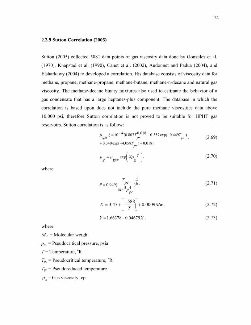
74
2.3.9 Sutton Correlation (2005)
Sutton (2005) collected 5881 data points of gas viscosity data done by Gonzalez et al.
(1970), Knapstad et al. (1990), Canet et al. (2002), Audonnet and Padua (2004), and
Elsharkawy (2004) to developed a correlation. His database consists of viscosity data for
methane, propane, methane-propane, methane-butane, methane-n-decane and natural gas
viscosity. The methane-decane binary mixtures also used to estimate the behavior of a
gas condensate that has a large heptanes-plus component. The database in which the
correlation is based upon does not include the pure methane viscosities data above
10,000 psi, therefore Sutton correlation is not proved to be suitable for HPHT gas
reservoirs. Sutton correlation is as follow:
]018.0)058.4exp(340.0
)449.0exp(357.0618.0807.0[410
+−+
−−−=
prTprTprTgscξμ . (2.69)
⎟⎠⎞⎜
⎝⎛= Y
gXgscg ρμμ exp . (2.70)
where
61
)43(949.0
pcpMw
pcT=ξ . (2.71)
MwT
X 0009.0588.147.3 +⎥⎦⎤
⎢⎣⎡+= . (2.72)
XY 04679.066378.1 −= . (2.73)
where
Mw = Molecular weight
ppc = Pseudocritical pressure, psia
T = Temperature, oR
Tpc = Pseudocritical temperature, ˚R
Tpr = Pseudoreduced temperature
gμ = Gas viscosity, cp
75
gscμ = Low pressure gas viscosity, cp
gρ = Gas density, g/cc
ξ = Viscosity normalizing parameter
2.3.10 Viswanathan Correlation (2007)
Viswanathan (2007) used a Cambridge Viscosity SPL440 viscometer to measure the
viscosity of pure methane. He measured methane viscosity at temperature of 116, 152,
188, 224, and 260 oF and pressure from 4500 to 20000 psia. Using NIST values at
temperatures of 100, 150, 200, 250, 300, 350, and 400 oF and pressure from 5000 to
30000 psia with interval of 1000 psia, Viswanathan modified Lee-Gonzalez-Eakin
correlation as follows:
( )Ygg XK ρμ exp= . (2.74)
TM
TMK
w
w++−
−=
9.128.443
)2888.00512.5(*0001.0 832.1. (2.75)
where
wMT
X 3938.09437.3084
1166.6 ++−= ⎥⎦⎤
⎢⎣⎡ . (2.76)
XY 1563.05893.0 −= . (2.77)
where
gμ = Gas viscosity, cp
gρ = Gas density, g/cc
MW = Molecular weight
T = Temperature, oR
Summary, no measured gas viscosity at high pressure and high temperature is available
so far. Thus correlations derived from data obtaining at low-moderate pressure and
temperature cannot be simply extrapolated to high pressure and high temperature

76
conditions. Experiments that measure gas viscosity at high pressure and high
temperature must be conducted before we derived correlation that can predict gas
viscosity accurately. As a result, a correlation covered both low and high pressure and
temperature is highly recommended. But it needs measured data as its solid base.

77
CHAPTER III
OBJECTIVE
Because a good correlation needs a wide range viscosity data as its cornerstone, the lack
of methane and nitrogen viscosity at HPHT required we put enormous effort towards the
viscosity of pure methane and nitrogen at HPHT. By adding methane and natural gas
viscosity at high pressures and high temperatures, a new correlation can be derived to
predict gas viscosity at HPHT.
Another fact needed to be addressed is that more nitrogen is found as we move to high
pressure and high temperature reservoirs. High concentration nitrogen in natural gas
affects not only the heat value of natural gas but also gas viscosity, which is critical to
petroleum engineering. The importance of gas viscosity is seen in its contribution in the
resistance to the flow of a fluid both in porous media and pipes during gas production
and transportation. Nitrogen is also one of common inject gases in gas injection projects,
thus an accurate estimation of its viscosity is vital to analyze reservoir performance. Due
to lack of correlation for nitrogen viscosity and the fact that hydrocarbon viscosity
correlation is inappropriate for nitrogen viscosity, a new correlation that is tailored for
nitrogen viscosity will be derived based on our experimental data. It provides a good
approach to get nitrogen viscosity at HPHT.

78
CHAPTER IV
METHODOLOGY
4.1 Experiment Facility
As mention before we need viscosity at HPHT to develop a new correlation through
which accurate viscosity can be guaranteed. To fill the viscosity data we will put our
effort in measuring gas viscosity at HPHT through appropriate facility. Falling-body
principle is employed in setup our experimental facility. Dr. Teodoriu, Dr. McCain, Mr.
Anup Viswanathan, and Mr. Frank Platt (Viswanathan, 2007; Viswanathan and McCain,
2005; Viswanathan et al., 2006) prepared and installed this delicate apparatus. The
facility consists of gas source, gas booster system, temperature control system,
measuring system, and data acquisition system. Figure 4-1 shows the setup of apparatus.
Figure 4-2 illustrates the layout of facility. Following is a detail description of the
facility.
Figure 4-1. The setup of apparatus for this study

79 Figure 4-2. Schematic of experimental facility
Outlet Valve 2
Piston Chamber Electromagnetic Coil
Internal Temperature Probe
Inlet Tube
Outlet Tube
Pressure Gauge
Inlet Valve 1
Pressure Gauge
Outlet Valve 1
Cable to Computer
Inlet Valve 2
Gas Vent Valve
Gas Outlet Valve (To Sensor)
GB-30 Gas Booster
Pressure Gauge Air Operated Hydraulic Pump
Pressure Gauge
Gas Tank
Oil Reservoir
Air Regulator
Gas Outlet Valve
Gas Inlet Valve
Air Inlet
Return Line
Oil Release Valve
Val
ve A
Gas Vent Valve
Oven (Regulate Temperature)

80
4.1.1 Gas Source
The gas we used for viscosity measurement is nitrogen, methane, and air. A gas tank that
supplies low pressure gas is used as original source. Gas tank is connected to the inlet of
gas booster system where gas is compressed to high pressure for measurement. Through
gas booster system we can compress gas from 1000 psi to 25000 psi.
4.1.2 Gas Booster System
Since the gas tank cannot provide pressure required by experiment, a gas booster system
was used to compress the gases to high pressures that match the requirement. The gas
booster system is consisting of a hydraulic pump coupled with the gas booster cylinder
to increase the pressure of a given gas sample. The gas booster system as used in this
project was manufactured by High Pressure Equipment Company. It belongs to Model
GBS-30 (Figure 4-3) which means it is rated for use up to 30,000 psi and has a one-to-
one ratio. Displacement per stroke is 112 cubic inches (1835 ml). Model GBS-30 is
complete and ready to operate. All that is required is an air supply for the pump and a
commercially available container of compressed gas.
Figure 4-3. Gas booster system used to compress gas in this study

81
The gas booster system includes manual valves, air regulator, filter and lubricator, air
gauge, high pressure gauge, reservoir, oil filter, pump, gas booster and related high
pressure tubing and fittings. The two major parts are air operated hydraulic pump which
uses house air at a pressure of 70 psia to pump hydraulic oil out of the oil reservoir and
the gas booster cylinder which contains a piston to separate the oil and the gas.
Operation is by means of an air operated hydraulic pump which pressurizes one end of
the gas booster which then compresses the gas in the opposite end of the booster. To
accomplish this, the gas inlet valve is opened to permit gas to fill the gas end of the
booster. Check valves are provided to permit gas flow in one direction only. With the
gas outlet valve open, the hydraulic pump is operated in order to pressurize the hydraulic
end of the booster. Thus, the gas is compressed in the booster. If required pressure is not
reached by the end of the stroke, the gas booster can easily be recycled for additional
strokes. Note the gauge on these systems is connected to the hydraulic side of the
booster. On the Model GBS-30 which has a 1 to 1 ratio, there is a direct reading of the
pressure in the gas end of the booster.
There are some drawbacks with the proto gas booster system. One of them is that the
rate of release of high pressure gas from the system is hard to be regulated, whereas the
gas outlet valve supplied is inadequate for this measure of control. Another difficulty is
the rate of release of oil from the gas booster cylinder cannot be controlled accurately.
An excessively rapid drop in pressure can cause the o-rings in the gas booster cylinder to
disintegrate and this can have dangerous implications. In order to improve the system to
be more efficient and safe, some changes were made to the gas booster system in the
laboratory. An extra pressure transducer was attached to the gas line since the main
pressure gauge on the gas booster system was connected to the oil line and this only
approximately described the true gas pressure. A couple of micro-tip controlled valves
were installed to help in carefully regulating the high pressure gas, and the vented oil.
82
Followings are the steps to operate the gas booster system:
1) All the valves are initially closed. The cylinder which contains the gas sample is
connected to the inlet of the gas booster system and cranked open. The inlet
valve in the gas booster system is also opened. All other valves are in the close
position. Gas starts to fill in the gas booster cylinder pushing the piston down.
2) The oil vent valve is now opened to allow for any remaining hydraulic oil in the
gas booster cylinder to trickle into the oil reservoir. This ensures that the cylinder
is now completely filled with the gas sample alone. The gas inlet valve is now
closed.
3) Valve A, the master valve for supplying air to the pump is opened and then the
air regulator is slowly opened to the desired level. This sets the pump in motion
and oil starts coming in from the bottom of the gas booster cylinder. The oil vent
valve should now be closed to allow the oil to accumulate in the cylinder.
4) On opening the air regulator further, more and more oil passes into the gas
booster cylinder from the oil reservoir. This causes a reduction of volume of the
gas sample thus increasing the pressure.
5) When the desired pressure has been reached, both Valve A and the air regulator
should be closed so that the pressure does not keep increasing.
6) The gas outlet valve can now be opened to supply high pressure gas as required.
7) When the experiments have ceased, the oil vent valve is now carefully opened to
release the oil back into the reservoir. This causes an increase in volume of the
gas and causes the pressure to go down.
8) The gas vent valve can now be opened to purge any remaining gas from the
system.
The high pressure gas from the gas booster system is now available to be connected to
the measurement sensor for the measurement of gas viscosity.

83
4.1.3 Temperature Control System - Oven
The temperature of the measuring system is controlled by a mechanical convection oven,
which was manufactured by Yamato Scientific America Inc. The measuring system was
placed inside the oven. The oven mode is DKN400 (Figure 4-4) with electric capacity of
115V AC, 12A and temperature setting range from 0 to 320 oC . The overheat protection
function incorporated into the oven prevents the damage to oven and measuring system
in case of human error. With this oven we can manipulate the measuring temperature as
we want. One drawback of this setup is that it usually takes 5 to 6 hours for temperature
reaching constant when we change to a new temperature own to the fact that the
convection medium used to transfer heat to measuring system is air.
Figure 4-4. The temperature control system in this study
4.1.4 Measurement System - Cambridge Viscometer
Every type of viscometer has its advantages and disadvantages. In this research a
modified falling body viscometer is used to measure gases viscosity at HPHT. The
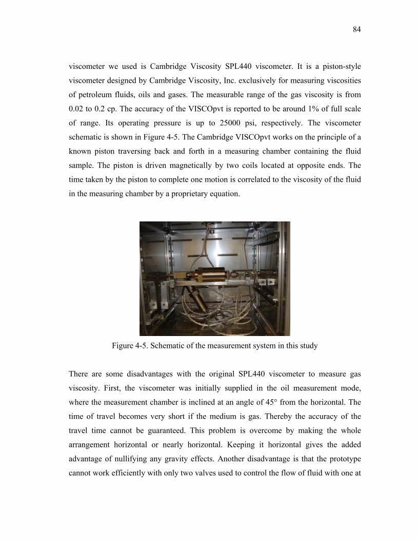
84
viscometer we used is Cambridge Viscosity SPL440 viscometer. It is a piston-style
viscometer designed by Cambridge Viscosity, Inc. exclusively for measuring viscosities
of petroleum fluids, oils and gases. The measurable range of the gas viscosity is from
0.02 to 0.2 cp. The accuracy of the VISCOpvt is reported to be around 1% of full scale
of range. Its operating pressure is up to 25000 psi, respectively. The viscometer
schematic is shown in Figure 4-5. The Cambridge VISCOpvt works on the principle of a
known piston traversing back and forth in a measuring chamber containing the fluid
sample. The piston is driven magnetically by two coils located at opposite ends. The
time taken by the piston to complete one motion is correlated to the viscosity of the fluid
in the measuring chamber by a proprietary equation.
Figure 4-5. Schematic of the measurement system in this study
There are some disadvantages with the original SPL440 viscometer to measure gas
viscosity. First, the viscometer was initially supplied in the oil measurement mode,
where the measurement chamber is inclined at an angle of 45° from the horizontal. The
time of travel becomes very short if the medium is gas. Thereby the accuracy of the
travel time cannot be guaranteed. This problem is overcome by making the whole
arrangement horizontal or nearly horizontal. Keeping it horizontal gives the added
advantage of nullifying any gravity effects. Another disadvantage is that the prototype
cannot work efficiently with only two valves used to control the flow of fluid with one at

85
the inlet tube and another at the outlet tube. These two valves are installed far away from
the cell. Therefore it requires large volume of test sample. This installation also increases
the time for gas to reach equilibrium considering the pressure difference between two
ends of the cell caused by the movement of piston. Dr. Teodoriu modified the
configuration of the original design by one pressure gauge at the inlet (very close to the
cell), one more valve at the inlet, and one more valve at the outlet. This modification
drastically reduces the time to reach equilibrium and cut down the required volume of
test sample to 30-40 %. Pressure gauge close to the cell provides more accurate data than
before.
The general procedures to operate the viscometer are:
1) After the installation of the whole experiment facility and gas in gas booster
system had been compressed and ready to be used, connect the inlet end of the
viscometer to the outlet line of the gas booster system.
2) Adjust the sensor’s temperature to the desired temperature by regulating the oven
temperature.
3) Open outlet valve of viscometer; open inlet valve of viscometer; open the outlet
valves at the gas booster system. Let the gas from gas booster system purge the
existing gas in the chamber and flow line for about one minute.
4) Now close the outlet valve of viscometer; keep inlet valve of viscometer open to
fill the chamber with measured gas until the pressure reaches the desired value.
5) Close inlet valve of viscometer; wait for the temperature in the chamber becomes
constant.
6) Adjust the pressure to the measured pressure; close the outlet valve of
viscometer; close the inlet valve of viscometer.
7) Start to measure gas viscosity at certain pressure and temperature.
8) After finish one measurement, keep temperature constant and change pressure to
other value to continue another measurement.

86
9) When the experiment finishes, close the outlet valves at the gas booster system;
close the inlet valve of viscometer; open outlet valves to vent gas.
4.1.5 Data Acquisition System
The Cambridge viscometer was also supplied with RS-232 serial communication
support, allowing the data measured by the viscometer to be synchronized with a
desktop computer. We setup a new recording control panel through which the
measurement is controlled (Figure 4-6). This gives the provision to save the data for later
analysis. The software used to record the measured data is ViscoLab. Through data
acquisition system we can output measured pressure, average temperature, average gas
viscosity, current temperature, and current gas viscosity. The measured interval can be
adjusted as requirement. With this system, manual recording of the experiment is not
necessary and large storage of measurement data becomes feasible.
Figure 4-6. Recording control panel to control the experiment
4.2 Experiment Procedure
The measurement in this stage is limited to nitrogen and methane. We started experiment
with measuring nitrogen viscosity considering safety and easy calibration. Constrained

87
by the viscometer measurement capacity of 0.02-0.2 cp and the viscometer rated
pressure of 25000 psig, we selected 3000 psi as the minimum pressure and 25000 psig as
the maximum for nitrogen. After finishing some experiments or particular time interval,
the facility was disassembled and all components were cleaned. These were done
because after particular period there are some contaminants trapped inside the chamber
and piston (Figure 4-7) will introduce system error to the measurement. After the
cleaning, all parts were assembled and ready to be used immediately. As we finished the
experiment on nitrogen viscosity, we switched to methane viscosity. We selected 4000
psi as the minimum pressure and 25000 psig as the maximum for methane because the
viscometer cannot provide accurate data at pressure less than 4000 psig.
Figure 4-7. Contaminants trapped on the piston
We decide the measurement procedure according to 1) the time required reaching
temperature equilibrium in measurement system is much longer than the time to reach
pressure equilibrium in the system, while the time for pressure reaching equilibrium
takes less than 10 seconds, 2) safety and data calibration requirements, 3) the viscometer
rated pressure and temperature, and 4) enough measuring data point to develop viscosity
Contaminants
Contaminants
Piston Piston

88
correlation. Therefore temperature will be the same and only the pressure is changed in
an experiment. After completing one experiment, we change to another temperature.
The following steps are used to implement our experiments:
1) We start experiment on measuring nitrogen viscosity. The first experiment is at
lowest temperature.
2) Set the temperature at the desired value and wait until temperature in the
measuring system becomes constant. This may take 5-7 hours.
3) In an experiment, we begin the measurement from lowest pressure of 3000 psi
and keep temperature constant. The measurement of viscosity at particular
pressure and temperature usually lasts 15-30 minutes.
4) Increase the pressure by 500 psi while keep temperature stable, measure viscosity
at this pressure and temperature for 15-30 minutes.
5) Continue the measurement by increasing the pressure until we reach the highest
pressure, which is ≤ 25000 psig, and always keep temperature constant during
this step, then measure viscosity at this pressure and temperature for 15-30
minutes.
6) Decrease the pressure by 500 psi and keep temperature constant at the same time,
and then measure viscosity at this pressure and temperature for 15-30 minutes.
7) Keep reducing pressure until touching the lowest pressure and keep temperature
constant at the same time, again measuring time for each pressure and
temperature is 15-30 minutes. So far we finish one experiment.
8) Steps 3-7 are repeated several times to understand the repeatability of the
measurement, i.e., we measure viscosity at same pressure and temperature
several times.
9) Through Steps 3-8 we finish the measurement for one temperature. We change
the temperature and wait 5-7 hours until it becomes constant, then repeat Steps 3-
8 to get viscosity for this new temperature.

89
10) Continue to more temperatures until we finish measurement of nitrogen
viscosity.
11) Upon completing nitrogen viscosity measurement we transfer to methane and
repeat the same step we measure nitrogen viscosity.
The cleaning of the viscometer is dependent on the number of experiments or the
viscometer running time. Repeated measurement provides abundant data for calibration
in the data analysis.
4.3 Measurement Principle of Viscometer in This Study
The knowledge of geometry of measuring cell is important to understand the principle
behind the measurement. The cell is a cylinder-shaped chamber with a piston inside
(Figures 4-1 and 4-8). Table 4-1 lists the dimension of chamber and piston.
Figure 4-8. Piston moves inside of chamber of viscometer using in this study
Dchamber θ
p1 p2
L v
Dpiston

90
Table 4-1. The dimension of chamber and piston (Malaguti and Suitter, 2010)
Piston Overall Length of Piston (Include the cone) 0.9412 inches Length of piston flank(rectangle part, exclude height of cone) 0.87658 inches Outer diameter of Piston 0.312 inches Base angle of the cone (θ) 22.5 degree Height of the cone 0.06462 inches Surface area of the cone(exclude base area) 0.07808 in2 Surface area of the piston flank (exclude the base and cone) 5.50773 in2 Weight of piston 4.807 g Chamber Inner diameter of chamber 0.314 inches Length of chamber 1.4 inches
In our study, the viscometer is placed horizontally. Therefore the chamber and piston are
in horizontal position. Figure 4-8 shows the cut away view of chamber inside which a
piston is moving from left to right. The piston is driven by an electromagnetic force. For
simplification, the following assumptions are made:
1) The time to accelerate is negligible or very short time for piston from static to
reach constant speed. This is because the acceleration time is very small
compared to the 2-way piston travel time. The flow in annulus is steady-state
flow.
2) A known, constant electromagnetic force applied during one way travel.
3) Piston is moving in the center of chamber and does not touch the chamber wall.
4) Fourth assumption is that both piston and chamber built from same material and
have same roughness.
5) The test fluid is Newtonian.
6) Gas viscosity is uniform throughout the chamber. Actually the pressure
difference between two ends of piston is 0-10 psi, which is very small comparing
with 3000-25000 psig measuring pressure, thus the variation of viscosity with
pressure can be neglected. So does the density.

91
7) Pressure drop along the annulus between piston and chamber is mainly friction
pressure drop, and the contribution from kinetic energy change is so small that it
is negligible.
8) For the laminar flow there is no slip on the surfaces of chamber and piston.
Assumption 7) can be proved by the first law of thermodynamics or the principle of
conservation of energy based on the uniform constructions of chamber and piston and
the pressure difference in assumption 6).
Forces on piston can be analyzed in two dimensions, horizontal and vertical directions.
For the purpose of this study, vertical forces are not considered. In horizontal direction,
when the piston moves with a constant velocity, v, the pressure in front of the piston is
higher than that behind the piston. In addition, the fluid flowing from the front of piston
through the annulus between piston and chamber wall to back of piston results in the
drag forces on the cone and flank of piston. Because the chamber and piston are in
horizontal position, the potential energy change is zero. As a result the piston is
subjected to five forces, the electromagnetic force, the drag force on the cone surface,
the drag force on the flank of the piston, the fluid forces in front of and behind the
piston. According to the force equilibrium, we have the following form.
frontflankpistonconepistonbehindem FDFDFFF ++=+ (4.1)
where
emF = Electromagnetic force,
conepistonDF = Drag force on the cone surface,
flankpistonDF = Drag force on the flank of the piston,
frontF = Fluid force in front of the piston,
behindF = Fluid force behind the piston.
The fluid force behind the piston is
1
2
1 4p
DApF piston
basepistonbehind π== (4.2)

92
where
1p = Pressure behind the piston,
basepistonA = Area of base of piston.
The fluid force in front of the piston is
2
2
22 4p
DApApF piston
basepistonbaseconefront π=== (4.3)
where
2p = Pressure in front of the piston,
baseconeA = Area of base of cone.
The drag force on the flank of the piston can be derived according to the flow regime of
fluid flowing around the piston. The drag force will be analyzed in two cases. One is
laminar flow and another is turbulent flow. When piston moves at a constant velocity the
volume of the fluid displaced by the piston is equal to the volume flows through the
annulus during a specific time interval, Δt. we have
displaceddisplacing VV = (4.4)
where
displacingV = Displacing volume when piston moves ahead,
displacedV = Displaced fluid volume that flows through annulus and back to the behind of
piston.
The displacing and displaced volumes can be expressed by
annulusflowfluidbasepistondisplacing ALAL = (4.5)
in terms of travel distance and cross section area.
where
displacingL = Travel distance of piston during a specific time interval,
flowfluidL = Travel distance of fluid flow in annulus during a specific time interval,
annulusA = Cross section area of annulus.

93
Replacing travel distance with velocity and time interval and knowing that annulus area
is the difference between chamber cross section area and piston base area, we obtain
( )basepistonchamberfluidbasepistonpiston AAtvtAv −Δ=Δ (4.6)
where
pistonv = Piston velocity,
fluidv = Mean fluid flow velocity,
Cancelling out the same term on both hand sides and expressing area in diameter results
in
⎟⎠⎞
⎜⎝⎛ −= 222
444 pistonchamberfluidpistonpiston DDvDv πππ (4.7)
where
pistonD = Piston diameter,
chamberD = Chamber diameter,
After several rearrangement of Equation 4.7 we come up with
( )22
2
pistonchamber
pistonpistonfluid DD
Dvv
−= (4.8)
It should be noted that fluid velocity in Equation 4.8 is average velocity in the annulus.
In our case, the diameter of piston and chamber are 0.312 and 0.314 inches, respectively.
Therefore the average fluid velocity is 77.75 times of piston velocity. For the case of
laminar flow, we assume fluid velocities on piston and chamber walls are zero and reach
maximum in the center of annulus. Bourgoyne et al. (1986) provide an analytical
solution for the pressure drop along the annulus. Now we consider a control fluid
volume in the annulus, which can be represented by rectangular slot flow as far as the
ratio of piston diameter to chamber diameter exceeds 0.3. In our case the ratio is
0.312/0.314, which is much higher than 0.3. Now consider a rectangular slot with an
area of A and height of h used to represent the annular flow in our apparatus (Figure 4-
9). The area and height can be expressed in diameters, which are

94
( )22
4 pistonchamber DDWhA −==π
(4.9)
where
( )pistonchamber DDW +=2π (4.10)
and
( )pistonchamber DDh −=21 (4.11)
Figure 4-9. Representing the annulus as a slot: (a) annulus and (b) equivalent slot, after
Bourgoyne et al. (1986)
Figure 4-10. Free body diagram for controlled fluid volume in a slot, after Bourgoyne et
al. (1986)
F2
F4 Δw
D
y
F3
ΔL y
vv0 τ
τh
Δy
F1
Piston wall
Chamber wall
p1 p2
y=h
y=0 τ0
h
h
πDpiston
W
πDchamber
Dchamber
Dpiston
(b) (a)

95
We deal with a controlled fluid volume (Figure 4-10) with width Δw and thickness Δy.
According to Bourgoyne et al. (1986), Force equilibrium in horizontal direction gives
3241 FFFF +=+ (4.12)
where
ywpF ΔΔ= 11 (4.13)
ywLdLdp
pywpF f ΔΔ⎟⎟⎠
⎞⎜⎜⎝
⎛Δ+=ΔΔ= 122 (4.14)
LwF y ΔΔ= τ3 (4.15)
and
LwydydLwF yyy ΔΔ⎟⎟
⎠
⎞⎜⎜⎝
⎛Δ+=ΔΔ= Δ+
τττ4 (4.16)
where
LΔ = Length of controlled fluid volume,
τ = Shear stress,
dLdp f = Frictional pressure gradient in annulus,
dydτ = Shear stress gradient in y direction,
Substituting Equations 4.13 through 4.16 into Equations 4.12 yields
Lw
ywLdL
dppLwy
dydywp
y
fy
ΔΔ+
ΔΔ⎟⎟⎠
⎞⎜⎜⎝
⎛Δ+=ΔΔ⎟⎟
⎠
⎞⎜⎜⎝
⎛Δ++ΔΔ
τ
ττ 11 (4.17)
Expanding and cancelling out the same terms on both sides gives
ywLdLdp
Lwydyd f ΔΔΔ=ΔΔΔ
τ (4.18)
Dividing Equations 4.18 by Lwy ΔΔΔ , we have
dLdp
dyd f=
τ (4.19)

96
Because dpf/dL is not a function of y, Equation 4.19 can be integrated with respect to y.
Separating variables and integrating gives
0ττ +=dL
dpy f
(4.20)
where τ0 is the constant of integration that corresponds to the shear stress at y=0. From
the definition of shear rate, γ& , we obtain
dydv
−=γ& (4.21)
Combining Equations 4.21 with the definition of viscosity for Newtonian fluid gives
0τμγμτ +=−==dLdp
ydydv f& (4.22)
where
μ = Newtonian fluid viscosity,
v = Newtonian fluid velocity,
Again, separating variable and integrating yields
00
2
2vy
dLdpyv f +−−=
μτ
μ (4.23)
where v0 is the second constant of integration that corresponds to the fluid velocity at
y=0. Applying the boundary condition
00 =v at y=0, (4.24)
we have
00
2 0200 v
dLdp f +−−=
μτ
μ (4.25)
Similarly applying the boundary condition
00 =v at y=h, (4.26)
we have
00
2
20 vh
dLdph f +−−=
μτ
μ (4.27)
Therefore, the constants of integration v0 and τ0 are

97
00 =v (4.28)
and
dLdph f
20 −=τ . (4.29)
Substituting Equations 4.28 and 4.29 into 4.23 gives
( )2
21 yhy
dLdp
v f −=μ
(4.30)
The flow rate q is the product of velocity v and area A. Integrating the controlled volume
flow rate throughout the interval 0 to h and recalling Equation 4.30 we obtain total flow
rate
( )∫∫∫ −===h
fhh
dyyhydLdpWvWdyvdAq
0
2
00 2μ (4.31)
Integrating Equations 4.31 yields
dLdpWhq f
μ12
3
= (4.32)
Substituting Equations 4.10 and 4.11 into 4.32, we obtain
( )( )222
192 pistonchamberpistonchamberf DDDD
dLdp
q −−=μ
π (4.33)
Expressing the flow rate in terms of the mean flow velocity and solving for the frictional
pressure gradient gives
( )( )
( )22
222
4
192
pistonchamber
pistonchamberpistonchamberf
fluid
DD
DDDDdLdp
Aqv
−
−−== π
μπ
or
( )2
48
pistonchamber
fluidf
DD
vAq
dLdp
−==
μ. (4.34)

98
Integrating Equation 4.34 and recalling ( )22
2
pistonchamber
pistonpistonfluid DD
Dvv
−= we have friction
pressure drop along the annulus
( )
( )( )
( ) ( )pistonchamberpistonchamber
flankpistonpistonpiston
pistonchamber
flankpistonpistonchamber
pistonpiston
pistonchamber
flankpistonfluidL
f
DDDD
LDv
DD
LDD
Dv
DD
LvdL
dLdp
ppflankpiston
+−=
−
⎥⎥⎦
⎤
⎢⎢⎣
⎡
−=
−==− ∫
3
2
2
22
2
20
12
48
48
48
μ
μ
μ
(4.35)
Substituting Equations 4.11 and 4.34 into 4.29 we have shear stress on piston wall,
which is opposite to the shear stress on fluid.
( )
pistonchamber
fluid
pistonchamber
fluidpistonchamberf
DDv
DD
vDDdL
dph
−=
−
−=⎟⎟
⎠
⎞⎜⎜⎝
⎛−−=−
μ
μτ
12
4842 20
(4.36)
Thus the drag force on the flank of the piston, flankpistonDF , is
( )pistonchamber
fluidflankpistonpistonflankpistonflankpiston DD
vLDADF
−=−=
μπτ
120
(4.37)
for laminar flow.
where
flankpistonL = Length of piston flank.
If flow in the annulus is turbulence, the drag force on the flank of the piston can be
analyzed by employing Reynolds number and friction factor.

99
Figure 4-11. Schematic of fluid flow through an annulus between piston and chamber
For Figure 4-11, force balance requires that
( )flankpistonchamberchamberflankpistonpistonpiston
flankpistonchamberannulus
LDLD
DFDFApp
πτπτ +=
+=− 12 (4.38)
Since piston diameter is very close to chamber diameter and basing on symmetrical
geometry, we have following observations
pistonchamber ττ = , (4.39)
and
pistonchamber DD ≅ . (4.40)
Therefore, we obtain
flankpistonchamber DFDF ≅ (4.41)
and
( ) ( ) ( )chamberpistonflankpistonpistonpistonchamber DDLDDpp +=−− πτπ 2212 4
(4.42)
or
( )( )pistonchamber
piston
flankpiston DDLpp
−=
− τ412 (4.43)
Introducing the definition of the Fanning friction factor (Wikipedia, 2009), f, which is
the ratio of the shear stress on the tubular wall applied by unit volume of fluid to its
kinetic energy.
p1 p2 Dchamber Dpiston
L
vfluid

100
fluidvolumeenergykineticfluidvolumewalltheonstressshearf = (4.44)
or
2
21
fluidf
chamberpiston
vf
ρ
ττ += . (4.45)
where
fρ = Fluid density.
Recalling chamberpiston ττ = , we have
2
41
fluidfpiston vfρτ = (4.46)
The fanning friction factor for smooth pipe, which is as in our case, and a Reynolds
number range of 2,100 to 100,000, can be approximated by the following form (Blasius,
1913):
25.0Re
0791.0N
f = (4.47)
where NRe is the Reynolds number, which is expressed as:
μρvD
N ffluide=Re (4.48)
where
eD = Equivalent circular diameter,
The equivalent circular diameter De is equal to four times the hydraulic radius rH.
He rD 4= (4.49)
and the hydraulic radius is defined as the ratio of the cross-sectional area to the wetted
perimeter of the flow channel. In our case it is
( )( ) 4
422
pistonchamber
chamberpiston
pistonchamber
H
DDDD
DDr
−=
+
−=
π
π
(4.50)
Substituting Equation 4.50 into 4.49, we have

101
( )pistonchamber
pistonchambere DD
DDD −=
−=
44 (4.51)
Substituting Equation 4.51 into 4.48, we have ( )
μρvDD
N ffluidpistonchamber −=Re (4.52)
Substituting Equation 4.52 into 4.47, we have
( ) 25.00791.0
⎥⎥⎦
⎤
⎢⎢⎣
⎡ −=
μρvDD
fffluidpistonchamber
(4.53)
Substituting Equation 4.53 into 4.46, we have
( )2
25.00791.0
41
fluidf
ffluidpistonchamber
piston v
μρvDD
ρτ
⎪⎪
⎭
⎪⎪
⎬
⎫
⎪⎪
⎩
⎪⎪
⎨
⎧
⎥⎥⎦
⎤
⎢⎢⎣
⎡ −= (4.54)
Simplifying Equation 4.54 yields
( ) 25.0
75.125.075.00198.0
pistonchamber
fluidfpiston
DD
v
−=
μρτ (4.55)
Thus the drag force on the flank of the piston, flankpistonDF , is expressed as
( ) 25.0
75.125.075.00198.0
pistonchamber
fluidfflankpistonpistonflankpistonpistonflankpiston
DD
vLDADF
−==
μρπτ (4.56)
for turbulent flow in annulus.
The drag force on the cone surface, conepistonDF , can be estimated by applying Stokes’ law
(Castleman, 1926). Figure 4-8 illustrates a piston traveling through a homogeneous fluid.
If the motion of the sphere is sufficiently slow, the inertia terms become negligible.
Under this condition the cone of the piston experience a drag force resulting from the
viscous fluid flow around the cone surface. The magnitude of drag force is dependent on
the flow regime, laminar or turbulent flow.

102
For laminar flow, the drag force is calculated from Stokes law. Stokes law has shown
that for creeping flow (Castleman, 1926) (i.e., the streamlines of fluid movement pass
smoothly about the particle and there is no eddying downstream of it) the drag force is
related to the piston velocity through the fluid by:
pistonpistonconepiston vDDF μπ3= . (4.57)
This equation is found to give acceptable accuracy for Reynolds numbers below 0.1. For
Reynolds numbers greater than 0.1, empirically determined friction factors must be used.
In case of turbulent flow, the concept of friction factor is introduced to estimate drag
force. It is defined by:
k
conepiston
AEDF
f = . (4.58)
Then the drag force can be expressed as:
kconepiston AEfDF = (4.59)
where
=A Characteristic area of the cone,
=kE Kinetic energy per unit volume.
The characteristic area of the cone in our case is given by:
2
41
pistonDA π= . (4.60)
The kinetic energy per unit volume is given by:
2
2pistonf
k
vE
ρ= . (4.61)
The friction factor f is a function of the Reynolds number and, in the case of non-
spherical shapes, a term called the sphericity. Sphericity, ψ, is defined as the surface area
of a sphere containing the same volume as the particle divided by the surface area of the
particle. In our case the particle is a cone with following geometry:
Base diameter =Dpiston,
Angle between base and flank = 22.5 degree, thus height of the cone is
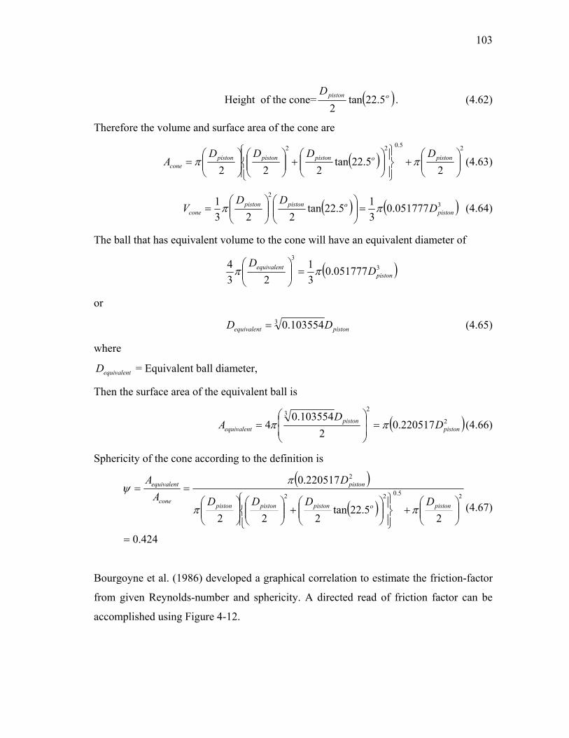
103
Height of the cone= ( )opistonD5.22tan
2. (4.62)
Therefore the volume and surface area of the cone are
( )25.022
25.22tan
222 ⎟⎟⎠
⎞⎜⎜⎝
⎛+
⎪⎭
⎪⎬⎫
⎪⎩
⎪⎨⎧
⎟⎟⎠
⎞⎜⎜⎝
⎛+⎟⎟
⎠
⎞⎜⎜⎝
⎛⎟⎟⎠
⎞⎜⎜⎝
⎛= pistonopistonpistonpiston
cone
DDDDA ππ (4.63)
( ) ( )32
051777.0315.22tan
2231
pistonopistonpiston
cone DDD
V ππ =⎟⎟⎠
⎞⎜⎜⎝
⎛⎟⎟⎠
⎞⎜⎜⎝
⎛= (4.64)
The ball that has equivalent volume to the cone will have an equivalent diameter of
( )33
051777.031
234
pistonequivalent D
Dππ =⎟⎟
⎠
⎞⎜⎜⎝
⎛
or
pistonequivalent DD 3 103554.0= (4.65)
where
equivalentD = Equivalent ball diameter,
Then the surface area of the equivalent ball is
( )2
23
220517.02
103554.04 piston
pistonequivalent D
DA ππ =⎟
⎟⎠
⎞⎜⎜⎝
⎛= (4.66)
Sphericity of the cone according to the definition is
( )
( )
424.0
25.22tan
222
220517.025.022
2
=
⎟⎟⎠
⎞⎜⎜⎝
⎛+
⎪⎭
⎪⎬⎫
⎪⎩
⎪⎨⎧
⎟⎟⎠
⎞⎜⎜⎝
⎛+⎟⎟
⎠
⎞⎜⎜⎝
⎛⎟⎟⎠
⎞⎜⎜⎝
⎛==
pistonopistonpistonpiston
piston
cone
equivalent
DDDD
DA
A
ππ
πψ
(4.67)
Bourgoyne et al. (1986) developed a graphical correlation to estimate the friction-factor
from given Reynolds-number and sphericity. A directed read of friction factor can be
accomplished using Figure 4-12.

104
Figure 4-12. Friction factor vs. particle Reynolds number for particles of different
sphericities, after Bourgoyne et al. (1986)
Reynolds number is expressed as
μρ pistonpistonf Dv
N =Re . (4.68)
For the piston in our study, whose sphericity is 0.424, the relationship between friction
factor and Reynolds number can be expressed as ( ) ( )[ ]
2
2ReRe
log117434.0log78036.09068.1
log117434.0log78036.09068.1
10
10
⎥⎥
⎦
⎤
⎢⎢
⎣
⎡
⎟⎟
⎠
⎞
⎜⎜
⎝
⎛+⎟
⎟
⎠
⎞
⎜⎜
⎝
⎛−
+−
=
=
μ
ρ
μ
ρ pistonpistonfpistonpistonf DvDv
NNf (4.69)
Therefore the drag force on the cone surface is 2
log117434.0log78036.09068.122
108
⎥⎥⎦
⎤
⎢⎢⎣
⎡
⎟⎟⎠
⎞⎜⎜⎝
⎛+
⎟⎟⎠
⎞⎜⎜⎝
⎛−
⎟⎟⎠
⎞⎜⎜⎝
⎛=
μρ
μρ
πρpistonpistonfpistonpistonf DvDv
pistonpistonfconepiston
DvDF (4.70)
Including these forces into force balance Equation 4.1, we have
2
2
1
2
412
34
pD
DDvLD
vDpD
F piston
pistonchamber
fluidflankpistonpistonpistonpiston
pistonem π
μπμππ +
−+=+
or
( )12
2
412
3 ppD
DDvLD
vDF piston
pistonchamber
fluidflankpistonpistonpistonpistonem −+
−+= π
μπμπ (4.71)

105
for laminar flow, and
( ) 2
2
25.0
75.125.075.0
log117434.0log78036.09068.122
1
2
40198.0
108
42
pD
DD
vLD
Dv
pD
F
piston
pistonchamber
fluidfflankpistonpiston
DvDv
pistonpistonf
pistonem
pistonpistonfpistonpistonf
πμρπ
πρ
π
μ
ρ
μ
ρ
+−
+
⎟⎟⎠
⎞⎜⎜⎝
⎛=
+
⎥⎥
⎦
⎤
⎢⎢
⎣
⎡
⎟⎟
⎠
⎞
⎜⎜
⎝
⎛+⎟
⎟
⎠
⎞
⎜⎜
⎝
⎛−
or
( ) ( )12
2
25.0
75.125.075.0
log117434.0log78036.09068.122
40198.0
108
2
ppD
DD
vLD
DvF
piston
pistonchamber
fluidfflankpistonpiston
DvDv
pistonpistonfem
pistonpistonfpistonpistonf
−+−
+
⎟⎟⎠
⎞⎜⎜⎝
⎛=
⎥⎥⎦
⎤
⎢⎢⎣
⎡
⎟⎟
⎠
⎞
⎜⎜
⎝
⎛+
⎟⎟
⎠
⎞
⎜⎜
⎝
⎛−
πμρπ
πρ μρ
μρ
(4.72)
for turbulent flow.
Substituting Equation 4.8 into Equations 4.71 and 4.72 we obtain
( )
( )12
2
22
2
4
123
ppD
DDDD
DvLD
vDF
piston
pistonchamber
pistonchamber
pistonpistonflankpistonpiston
pistonpistonem
−+
−
−+=
π
μπμπ
(4.73)
for laminar flow, and
( )( )
( )12
2
25.0
75.1
22
225.075.0
log117434.0log78036.09068.122
4
0198.0
108
2
ppD
DD
DDD
vLD
DvF
piston
pistonchamber
pistonchamber
pistonpistonfflankpistonpiston
DvDv
pistonpistonfem
pistonpistonfpistonpistonf
−+
−
⎥⎥⎦
⎤
⎢⎢⎣
⎡
−+
⎟⎟⎠
⎞⎜⎜⎝
⎛=
⎥⎥
⎦
⎤
⎢⎢
⎣
⎡
⎟⎟
⎠
⎞
⎜⎜
⎝
⎛+⎟
⎟
⎠
⎞
⎜⎜
⎝
⎛−
π
μρπ
πρ μ
ρ
μ
ρ
(4.74)
for turbulent flow.

106
Again substituting Equation 4.35 into Equation 4.73 we obtain
( ) ( )
( ) ( )pistonchamberpistonchamber
flankpistonpistonpistonpiston
pistonchamberpistonchamber
pistonpistonflankpistonpistonpistonpistonem
DDDD
LDvD
DDDD
DvLDvDF
+−+
+−+=
3
22
2
2
484
123
μπ
μπμπ
or
( ) ( )pistonchamberpistonchamber
chamberpistonpistonflankpistonpistonpistonem
DDDD
DDvLvDF
+−+= 3
3123
μπμπ (4.75)
for laminar flow.
Recalling ( )( )pistonchamber
piston
flankpiston DDLpp
−=
− τ412 and 2
41
fluidfpiston vfρτ = , we have
( )( )
( )( )pistonchamber
pistonchamber
pistonpistonf
DvDv
pistonchamber
fluidf
flankpiston
DD
DDD
v
DD
vf
Lpp
pistonpistonfpistonpistonf
−
⎥⎥⎦
⎤
⎢⎢⎣
⎡
−=
−
⎟⎠⎞
⎜⎝⎛
=−
⎥⎥
⎦
⎤
⎢⎢
⎣
⎡
⎟⎟
⎠
⎞
⎜⎜
⎝
⎛+⎟
⎟
⎠
⎞
⎜⎜
⎝
⎛− 2
22
2log117434.0log78036.09068.1
2
12
2
10
414
ρ
ρ
μ
ρ
μ
ρ
or
( ) ( )23
42log117434.0log78036.09068.1
12
2
10
pistonchamberpistonchamber
flankpistonpistonpistonf
DvDv
DDDD
LDvpp
pistonpistonfpistonpistonf
+−=−
⎥⎥⎦
⎤
⎢⎢⎣
⎡
⎟⎟
⎠
⎞
⎜⎜
⎝
⎛+
⎟⎟
⎠
⎞
⎜⎜
⎝
⎛−
ρμ
ρμ
ρ
(4.76)
Again substituting Equation 4.76 into Equation 4.74 we obtain

107
( )( )
( ) ( )⎟⎟⎟⎟⎟
⎠
⎞
⎜⎜⎜⎜⎜
⎝
⎛
+−+
−
⎥⎥⎦
⎤
⎢⎢⎣
⎡
−+
⎟⎟⎠
⎞⎜⎜⎝
⎛=
⎥⎥⎦
⎤
⎢⎢⎣
⎡
⎟⎟
⎠
⎞
⎜⎜
⎝
⎛+
⎟⎟
⎠
⎞
⎜⎜
⎝
⎛−
⎥⎥⎦
⎤
⎢⎢⎣
⎡
⎟⎟
⎠
⎞
⎜⎜
⎝
⎛+
⎟⎟
⎠
⎞
⎜⎜
⎝
⎛−
23
42log117434.0log78036.09068.1
2
25.0
75.1
22
225.075.0
log117434.0log78036.09068.122
2
2
104
0198.0
108
pistonchamberpistonchamber
flankpistonpistonpistonf
DvDv
piston
pistonchamber
pistonchamber
pistonpistonfflankpistonpiston
DvDv
pistonpistonfem
DDDD
LDvD
DD
DDD
vLD
DvF
pistonpistonfpistonpistonf
pistonpistonfpistonpistonf
ρπ
μρπ
πρ
μρ
μρ
μρ
μρ
(4.77)
for turbulent flow.
Equations 4.75 and 4.77 are the governing equations for viscosity measurement in
laminar and turbulent flow. Now we consider the laminar flow case. Extracting pistonvμ
from terms on the right-hand side of Equation 4.75 yields
( ) ( )⎥⎥⎦
⎤
⎢⎢⎣
⎡
+−+=
pistonchamberpistonchamber
chamberpistonflankpistonpistonpistonem
DDDD
DDLDvF 3
3123
ππμ (4.78)
Piston velocity can be expressed as
tL
v chamberpiston = (4.79)
where
chamberL = Chamber length,
t = Piston travel time from one end of chamber length to the other,
Substituting Equation 4.79 into Equation 4.78 and recasting gives
( ) ( )⎥⎥⎦
⎤
⎢⎢⎣
⎡
+−+
=
pistonchamberpistonchamber
chamberpistonflankpistonpistonchamber
em
DDDD
DDLDL
tF
3
3123
ππ
μ (4.80)

108
Equation 4.80 indicates that under laminar flow condition fluid viscosity can be
estimated by recording the travel time, assuming the geometry of piston and chamber,
and electromagnetic force are given. After a thorough review of “viscous drag” paper
(Cambridge Viscosity Inc., 2010) provided by the manufacturer-Cambridge we found
that Cambridge derived an equation that is similar to Equation 4.80 for laminar flow. It
should be noted that the derivation in the “viscous drag” paper is not completely shown.
Therefore we cannot check its validity.
For turbulent flow, substituting Equation 4.79 into Equation 4.77 we have
( )( )
( ) ( )⎟⎟⎟⎟⎟
⎠
⎞
⎜⎜⎜⎜⎜
⎝
⎛
+−+
−
⎥⎥⎦
⎤
⎢⎢⎣
⎡
−+
⎟⎟⎠
⎞⎜⎜⎝
⎛=
⎥⎥
⎦
⎤
⎢⎢
⎣
⎡
⎟⎟
⎠
⎞
⎜⎜
⎝
⎛+⎟
⎟
⎠
⎞
⎜⎜
⎝
⎛−
⎥⎥
⎦
⎤
⎢⎢
⎣
⎡
⎟⎟
⎠
⎞
⎜⎜
⎝
⎛+⎟
⎟
⎠
⎞
⎜⎜
⎝
⎛−
223
42log117434.0log78036.09068.1
2
25.0
75.1
22
225.075.0
log117434.0log78036.09068.1
2
22
2
2
104
0198.0
108
tDDDD
LDLD
DD
DDtLD
LD
tDL
F
pistonchamberpistonchamber
flankpistonpistonchamberf
tDL
tDL
piston
pistonchamber
pistonchamber
chamberpistonfflankpistonpiston
tDL
tDL
pistonchamberfem
pistonchamberfpistonchamberf
pistonchamberfpistonchamberf
ρπ
μρπ
πρ
μ
ρ
μ
ρ
μ
ρ
μ
ρ
or
( ) ( )
( ) ( ) 223
26log117434.0log78036.09068.1
75.175.12
75.15.425.075.0
log117434.0log78036.09068.1
2
22
4
10
0198.0
108
2
2
tDDDD
LLD
tDDDD
LLD
tDL
F
pistonchamberpistonchamber
flankpistonchamberpistonf
tDL
tDL
pistonchamberpistonchamber
flankpistonchamberpistonf
tDL
tDL
pistonchamberfem
pistonchamberfpistonchamberf
pistonchamberfpistonchamberf
+−+
+−+
⎟⎟⎠
⎞⎜⎜⎝
⎛=
⎥⎥
⎦
⎤
⎢⎢
⎣
⎡
⎟⎟
⎠
⎞
⎜⎜
⎝
⎛+⎟
⎟
⎠
⎞
⎜⎜
⎝
⎛−
⎥⎥
⎦
⎤
⎢⎢
⎣
⎡
⎟⎟
⎠
⎞
⎜⎜
⎝
⎛+⎟
⎟
⎠
⎞
⎜⎜
⎝
⎛−
ρπ
μπρ
πρ
μ
ρ
μ
ρ
μ
ρ
μ
ρ
(4.81)

109
Since the viscosity, μ, cannot be separated from time, t, in Equation 4.81, the estimation
of viscosity can only be done by solving Equation 4.81 implicitly. A trial and error
method would be used to build a relationship between viscosity and travel time. After
the relationship is constructed viscosity can be measured by recording the one-way
travel time. Another difficulty for turbulent flow is that fluid density at interested
condition must be known. Therefore the measurement of fluid density need to be run
simultaneously, otherwise density will be calculated through an equation-of-states,
which requires the composition of fluid. To eliminate the complexity turbulent flow
should be avoided during the experiment. The manufacturer did not provided
information about the application of viscometer under the turbulent flow condition.
4.4 Calibration of Experimental Data
4.4.1 Raw data and the Manufacturer’s Converted Equation
Apparently the raw data from experiment is not true gas viscosity if we note the big
difference between raw viscosity data and NIST values in both methane and nitrogen
viscosity at different pressures and temperatures in Figures 4-13 through 4-16. The
manufacturer did not provide the proprietary equation that leads to the raw data.
Therefore we do not know the relationship between piston traveling time and raw
viscosity data in this black box. Since the raw measured viscosity reading directly from
the viscometer is not the true gas viscosity, the manufacturer of Cambridge viscometer
provided an equation to convert the raw data to what they believe is true gas viscosity.
The equation to correct the pressure effect is 875.2
, )/)*05-E61.4((* APAMpc += ηη . (4.82)
where
p = Pressure, psia
ηM = Measured viscosity, cp
ηc,p =P-corrected viscosity, cp

110
A = Annulus (measurement chamber diameter-piston diameter) in thousandths of an
inch.
For the viscometer we used, the measurement chamber diameter is 0.314 inches, piston
diameter is 0.312 inches. Therefore, A is
2100031203140 =−= )*..(A . (4.83)
As a result, the equation used to convert measured viscosity to corrected viscosity
becomes 875.2
, )2/)*50-E61.42((* PMpc += ηη . (4.84)
Figure 4-13. Comparison of raw viscosity data with NIST values for methane at
temperature of 100 oF

111
Figure 4-14. Comparison of raw viscosity data with NIST values for methane at
temperature of 250 oF
Figure 4-15. Comparison of raw viscosity data with NIST values for nitrogen at
temperature of 152 oF

112
Figure 4-16. Comparison of raw viscosity data with NIST values for nitrogen at
temperature of 330 oF
4.4.2 New Converted Equation to Convert Raw Data to True Viscosity
A close look at this equation indicates that it only considers the effect of pressure, and
omits temperature. Thus the validity of this equation is needed to be checked with the
available viscosity data. Comparing these converted data with NIST values for methane
viscosity at temperatures of 100 and 250 oF and nitrogen viscosity at temperatures of 152
and 330 oF indicated that these converted data are not true gas viscosities (Figures 4-17
through 4-20). It is noted that the converted viscosities deviate from NIST values for
both methane and nitrogen.

113
Figure 4-17. Comparison of pressure-converted methane viscosity with NIST values at
temperature of 100 oF
Figure 4-18. Comparison of pressure-converted methane viscosity with NIST values at
temperature of 250 oF

114
Figure 4-19. Comparison of pressure-converted nitrogen viscosity with NIST values at
temperature of 152 oF
Figure 4-20. Comparison of pressure-converted nitrogen viscosity with NIST values at
temperature of 330 oF

115
Since the equation provided by manufacturer cannot convert raw data into true viscosity,
a new calibration equation is necessary and vital. To be convenient, we denoted the
viscosity calculated from manufacturer’s equation as pressure-converted viscosity since
it only consists pressure correction. The viscosity calculated from the new calibration
equation we are going to develop is denoted as pressure-temperature-converted viscosity
because both pressure and temperature corrections are incorporated. To develop the new
equation we respect two facts: 1) obviously temperature plays a vital role. Its effect on
gas viscosity cannot be neglected. So it must be included into the converted equation as
pressure. 2) To honor gas viscosity at low-moderate pressure provided by former
investigators, we used their data as our calibration goal since these data are agree with
each other thus are accepted by most researchers. Since nitrogen and methane viscosity
at moderate pressure range, 3000 to 8000 psig, had been studied thoroughly and
accepted by people, we calibrated our data to the existing viscosity data at the range of
3000 to 8000 psig using pressure and temperature as variables in the calibrating
equation.
The development of new equation is shown in the following steps:
1) Candidate database for constructing new calibration equation
As mentioned above, nitrogen and methane viscosity at moderate pressure range,
3000 to 8000 psig, had been studied thoroughly and accepted by people, we
calibrated raw data to the existing viscosity data at those conditions using
pressure and temperature as variables in the calibrating equation.
2) Raw data pre-process
For the sake of high quality data acquisition, same temperature pressure
experiments are repeated. Two to seven experiments were run to check the
repeatability of the viscometer. Experiments with high repeatability are chosen as
the database to develop new calibration equation. Data recorded at unstable
pressure and temperature are removed. Outliers are excluded. After this pre-

116
process, only data with good quality are input into the database for generating the
new calibration equation.
3) Converting raw data using manufacturer’s equation
Although how manufacturer came up with Equation 4.82 is a black box to us. In
this work we kept Equation 4.82 to honor that manufacturer had corrected the
pressure effect on viscosity. But since they omitted the temperature effect, we
will implement what had left behind. Comparing pressure-converted viscosity
with NIST values at pressure range of 3000 to 8000 psi as shown in Figures 4-17
through 4-20 we found that there is a gap between pressure-converted viscosity
and true viscosity. So we need to find out a correlation that can convert the
pressure-converted viscosity to true viscosity. This can be done by rotating the
pressure-converted viscosity to the position that is parallel to true viscosity, and
then apply a vertical shift to make it overlap with the true viscosity at pressure
range of 3000 to 8000 psi.
4) Converting the pressure-converted viscosity to true viscosity
As said in step 3), the conversion requires a rotation and a vertical shift.
Mathematically a non-linear regression method is applied to get the correlation
due to two facts. a) the relation between slope of pressure-converted viscosity
and slope of NIST values is not a simple linear-relationship, and b) The vertical
shift is a function of temperature. The pressure-converted viscosities at different
pressure temperature are collected (Tables 4-2 and 4-4). NIST viscosity at
corresponding pressure temperature is also collected (Tables 4-3 and 4-5). A
statistical analysis gave that the following term
3014.7)-(*C)Ln(*C+)Ln(*C32
1 pTT
T⎥⎦⎤
⎢⎣⎡ +
where
p = Pressure, psia
T = Temperature, oF
C1, C2, and C3 = Coefficients
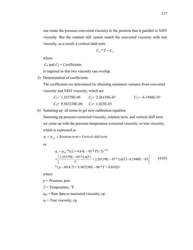
117
can rotate the pressure-converted viscosity to the position that is parallel to NIST
viscosity. But the rotation still cannot match the converted viscosity with true
viscosity, as a result, a vertical shift term
54 C+*C T
where
C4 and C5 = Coefficients
is required so that two viscosity can overlap.
5) Determination of coefficients
The coefficients are determined by obtaining minimum variance from converted
viscosity and NIST viscosity, which are
C1= 1.35379E-05 C2= 2.26139E-07 C3= -6.1948E-07
C4= 9.363238E-06 C5= 1.023E-03
6) Summing up all terms to get new calibration equation
Summing up pressure-corrected viscosity, rotation term, and vertical shift term
we come up with the pressure-temperature-corrected viscosity, or true viscosity,
which is expressed as
termshiftVerticaltermRotationpct ++= ,ηη
or
0.01023+*069.363238E+3014.7)-(*
076.1948E-)Ln(*072.26139E+)Ln(*051.35379E)2/)*05E61.42((* 875.2
Tp
TT
TPMt
−
⎥⎦⎤
⎢⎣⎡ −−
−+
−+=ηη
(4.85)
where
p = Pressure, psia
T = Temperature, oF
ηM = Raw data or measured viscosity, cp
ηt = True viscosity, cp

118
Table 4-2. Pressure-corrected nitrogen viscosity
Pressure Temperature (oF) (psia) 116 134 152 170 200 250 3014.7 0.01336 0.01324 0.01292 0.01271 0.01247 0.01212 3514.7 0.01425 0.01384 0.01368 0.01312 0.01299 0.01252 4014.7 0.01520 0.01443 0.01433 0.01410 0.01355 0.01312 4514.7 0.01597 0.01527 0.01516 0.01465 0.01400 0.01359 5014.7 0.01659 0.01581 0.01572 0.01540 0.01455 0.01409 5514.7 0.01749 0.01659 0.01655 0.01618 0.01514 0.01460 6014.7 0.01817 0.01722 0.01720 0.01683 0.01586 0.01507 6514.7 0.01888 0.01790 0.01804 0.01743 0.01639 0.01537 7014.7 0.01959 0.01861 0.01867 0.01792 0.01707 0.01576 7514.7 0.02038 0.01936 0.01923 0.01854 0.01764 0.01635 8014.7 0.02118 0.02015 0.01984 0.01912 0.01825 0.01694
Table 4-2. Continued
Pressure Temperature (oF) (psia) 260 280 300 330 350 3014.7 0.012035 0.011923 0.011835 0.01129 0.010814 3514.7 0.012456 0.012348 0.012175 0.011813 0.01123 4014.7 0.012892 0.012733 0.012485 0.011997 0.011939 4514.7 0.013247 0.012951 0.012718 0.012282 0.01228 5014.7 0.013565 0.013411 0.013201 0.012656 0.012453 5514.7 0.013873 0.013844 0.013507 0.013007 0.012727 6014.7 0.014261 0.014277 0.013856 0.013354 0.012908 6514.7 0.01466 0.014692 0.014293 0.013703 0.013301 7014.7 0.015177 0.01512 0.01471 0.013952 0.013624 7514.7 0.01569 0.01553 0.015247 0.01438 0.014048 8014.7 0.016218 0.015946 0.015544 0.014636 0.014334

119
Table 4-3. Nitrogen viscosity from NIST
Pressure Temperature (oF) (psia) 116 134 152 170 200 250 3014.7 0.02353 0.023724 0.023938 0.024169 0.024583 0.0253333514.7 0.024604 0.024731 0.024886 0.025065 0.025403 0.02605 4014.7 0.025723 0.025783 0.025878 0.026002 0.02626 0.0267994514.7 0.026874 0.026867 0.026901 0.02697 0.027147 0.0275765014.7 0.028047 0.027974 0.027948 0.027961 0.028058 0.0283755514.7 0.029231 0.029094 0.029009 0.02897 0.028986 0.0291916014.7 0.030421 0.030222 0.030081 0.029989 0.029927 0.0300216514.7 0.031611 0.031353 0.031157 0.031014 0.030875 0.0308627014.7 0.032798 0.032483 0.032234 0.032042 0.031829 0.0317097514.7 0.033978 0.03361 0.03331 0.033071 0.032786 0.0325628014.7 0.035152 0.034731 0.034383 0.034098 0.033743 0.033418
Table 4-3. Continued
Pressure Temperature (oF) (psia) 260 280 300 330 350 3014.7 0.025489 0.025806 0.026129 0.02662 0.026952 3514.7 0.026188 0.026473 0.026765 0.027216 0.027523 4014.7 0.026919 0.027169 0.02743 0.027838 0.02812 4514.7 0.027677 0.027891 0.028119 0.028483 0.028738 5014.7 0.028456 0.028634 0.028828 0.029147 0.029375 5514.7 0.029253 0.029394 0.029555 0.029828 0.030028 6014.7 0.030064 0.030168 0.030295 0.030522 0.030694 6514.7 0.030885 0.030953 0.031047 0.031228 0.031372 7014.7 0.031714 0.031746 0.031806 0.031942 0.032058 7514.7 0.032548 0.032545 0.032573 0.032663 0.032752 8014.7 0.033386 0.033348 0.033344 0.03339 0.033451

120
Table 4-4. Pressure-corrected methane viscosity
Pressure Temperature (oF) (psia) 100 120 140 160 180 188 200 4514.7 0.01180 0.01091 0.01008 0.00949 0.00892 0.00872 0.008445014.7 0.01304 0.01195 0.01098 0.01034 0.00995 0.00950 0.008945514.7 0.01394 0.01289 0.01149 0.01104 0.01062 0.01026 0.009596014.7 0.01547 0.01354 0.01231 0.01168 0.01124 0.01107 0.010466514.7 0.01591 0.01400 0.01341 0.01238 0.01184 0.01156 0.011027014.7 0.01622 0.01459 0.01415 0.01298 0.01236 0.01201 0.011637514.7 0.01711 0.01521 0.01500 0.01364 0.01283 0.01254 0.012188014.7 0.01774 0.01587 0.01558 0.01375 0.01354 0.01301 0.01269
Table 4-4. Continued
Pressure Temperature (oF) (psia) 220 225 230 250 260 280 4514.7 0.00802 0.007977 0.007837 0.007502 0.007343 0.0070725014.7 0.008687 0.008627 0.0085 0.007961 0.007856 0.0075055514.7 0.009226 0.009111 0.008954 0.008435 0.008353 0.007986014.7 0.009758 0.009669 0.009475 0.008902 0.008819 0.0084136514.7 0.010405 0.010208 0.009997 0.009339 0.009286 0.0088927014.7 0.010717 0.010633 0.010504 0.00983 0.009647 0.0092967514.7 0.011451 0.011093 0.010897 0.010291 0.010079 0.0096798014.7 0.011816 0.011747 0.011352 0.010727 0.010605 0.010097
Table 4-4. Continued
Pressure Temperature (oF) (psia) 300 320 340 360 380 415 4514.7 0.006833 0.006619 0.00615 0.006281 0.006134 0.0059425014.7 0.007186 0.006821 0.006531 0.006593 0.00639 0.0061765514.7 0.007579 0.007169 0.00709 0.006909 0.006657 0.0063766014.7 0.00794 0.007546 0.007484 0.00726 0.007018 0.0065916514.7 0.008369 0.007955 0.007757 0.007485 0.007176 0.0068857014.7 0.008705 0.008299 0.007987 0.007671 0.007413 0.0070847514.7 0.009026 0.008634 0.008245 0.007983 0.007652 0.0072948014.7 0.009376 0.008916 0.008583 0.008143 0.0079 0.007536

121
Table 4-5. Methane viscosity from NIST
Pressure Temperature (oF) (psia) 100 120 140 160 180 188 200 4514.7 0.02454 0.02377 0.02315 0.02265 0.02226 0.02212 0.021955014.7 0.02615 0.02529 0.02459 0.02401 0.02353 0.02337 0.023155514.7 0.02766 0.02674 0.02596 0.02531 0.02477 0.02458 0.024336014.7 0.02909 0.02811 0.02728 0.02657 0.02597 0.02576 0.025466514.7 0.03045 0.02941 0.02853 0.02777 0.02712 0.02688 0.026567014.7 0.03173 0.03065 0.02972 0.02892 0.02822 0.02797 0.027637514.7 0.03296 0.03184 0.03086 0.03002 0.02928 0.02902 0.028658014.7 0.03412 0.03297 0.03196 0.03108 0.03031 0.03003 0.02963
Table 4-5. Continued
Pressure Temperature (oF) (psia) 220 225 230 250 260 280 4514.7 0.021708 0.021658 0.021612 0.02146 0.021401 0.0213155014.7 0.022844 0.022778 0.022716 0.022503 0.022416 0.0222775514.7 0.023958 0.023877 0.0238 0.023533 0.02342 0.0232316014.7 0.025042 0.024949 0.024859 0.024541 0.024405 0.024176514.7 0.026095 0.025989 0.025888 0.025526 0.025367 0.0250917014.7 0.027113 0.026997 0.026886 0.026483 0.026305 0.0259917514.7 0.028098 0.027972 0.027852 0.027412 0.027217 0.0268688014.7 0.029049 0.028916 0.028786 0.028314 0.028102 0.027722
Table 4-5. Continued
Pressure Temperature (oF) (psia) 300 320 340 360 380 415 4514.7 0.021266 0.021246 0.021253 0.021282 0.021331 0.0214565014.7 0.022178 0.022113 0.022078 0.022069 0.022082 0.0221515514.7 0.023085 0.022978 0.022904 0.022858 0.022837 0.0228516014.7 0.023983 0.023835 0.023724 0.023643 0.023589 0.0235516514.7 0.024864 0.02468 0.024534 0.02442 0.024336 0.0242487014.7 0.025728 0.02551 0.025331 0.025187 0.025073 0.0249397514.7 0.026572 0.026322 0.026113 0.02594 0.0258 0.0256228014.7 0.027395 0.027116 0.026879 0.02668 0.026514 0.026294
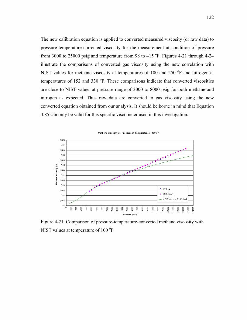
122
The new calibration equation is applied to converted measured viscosity (or raw data) to
pressure-temperature-corrected viscosity for the measurement at condition of pressure
from 3000 to 25000 psig and temperature from 98 to 415 oF. Figures 4-21 through 4-24
illustrate the comparisons of converted gas viscosity using the new correlation with
NIST values for methane viscosity at temperatures of 100 and 250 oF and nitrogen at
temperatures of 152 and 330 oF. These comparisons indicate that converted viscosities
are close to NIST values at pressure range of 3000 to 8000 psig for both methane and
nitrogen as expected. Thus raw data are converted to gas viscosity using the new
converted equation obtained from our analysis. It should be borne in mind that Equation
4.85 can only be valid for this specific viscometer used in this investigation.
Figure 4-21. Comparison of pressure-temperature-converted methane viscosity with
NIST values at temperature of 100 oF

123
Figure 4-22. Comparison of pressure-temperature-converted methane viscosity with
NIST values at temperature of 250 oF
Figure 4-23. Comparison of pressure-temperature-converted nitrogen viscosity with
NIST values at temperature of 152 oF

124
Figure 4-24. Comparison of pressure-temperature-converted nitrogen viscosity with
NIST values at temperature of 330 oF

125
CHAPTER V
EXPERIMENTAL RESULTS
5.1 Nitrogen Viscosity Measurement
The nitrogen is prepared by ACETYLENE OXYGEN Co.. The mole fraction of nitrogen
is 99.95%. Initial pressure in the gas tank is 1500 psig. Lots of efforts were investigated
on nitrogen viscosity. There are totally 91 tests on nitrogen viscosity. Measuring
condition is at pressures range from 3000 to 24500 psig with interval of 500 psi and at
temperatures of 99, 105, 109, 111, 116, 134, 152, 165, 170, 174, 187, 200, 250, 260,
280, 300, 330, and 350 oF. Table 5-1 lists the experiments we had done on measuring
nitrogen viscosity. Experiment data are used to develop the new converted equation. The
more experiments we did on nitrogen, the more confident we are on the new converted
equation. These experimental data are also used to develop a new gas viscosity
correlation that is specified for nitrogen viscosity.

126
Table 5-1. Statistic of nitrogen viscosity experiment in this study
Composition Temperature Pressure No. of Experiment oF psia
N2 99 3014.7-13514.7 4 N2 105 3014.7-14014.7 3 N2 109 3014.7-13514.7 3 N2 111 3014.7-14014.7 3 N2 116 3014.7-23014.7 7 N2 134 3014.7-22014.7 14 N2 151 3014.7-13514.7 3 N2 152 3014.7-24014.7 10 N2 165 3014.7-15514.7 3 N2 170 3014.7-23514.7 11 N2 174 3014.7-15014.7 4 N2 187 3014.7-17014.7 2 N2 200 3014.7-24514.7 6 N2 250 3014.7-22514.7 4 N2 260 3014.7-24514.7 6 N2 280 3014.7-24514.7 2 N2 300 3014.7-24514.7 2 N2 330 3014.7-23514.7 2 N2 350 3014.7-24514.7 2
5.2 Nitrogen Viscosity Analysis
Comparing lab data from this study with NIST values and data from other investigators
illuminated that extrapolating correlation based on low-moderate pressure/temperature to
HPHT yields unacceptable result. For all experiments on nitrogen viscosity, lab data
deviated from NIST value at high pressure at temperature of 116 oF (Figures 5-1 to 5-4).
Similar result can be observed for temperature of 134, 152, 170, 200, 250, 260, 280, 300,
330, and 350 oF as show in Figures A-1 to A-27 in Appendix A. The deviation of NIST
values from experimental data can be as high as 4.91% at pressure higher than 25014.7
psia. At high pressure nitrogen viscosities from lab are lower than NIST values. The
difference between lab data and NIST values increases as pressure increases. This

127
difference at high pressure indicates that existing correlation cannot provide accurate
viscosity to optimize the production of gas reservoirs with moderate-high nitrogen
concentration at HPHT.
Figure 5-1. Nitrogen viscosity vs. pressure at 116 oF (Test 68)
Figure 5-2. Nitrogen viscosity vs. pressure at 116 oF (Test 69)

128
Figure 5-3. Nitrogen viscosity vs. pressure at 116 oF (Test 70)
Figure 5-4. Nitrogen viscosity vs. pressure at 116 oF (Test 71)

129
Nitrogen, as a non-hydrocarbon, shows different thermodynamics properties from
normal paraffins. Its viscosity varying with pressure and temperature does not follow the
theorem of corresponding state as we see in hydrocarbon. So far no correlation is
available to estimate nitrogen viscosity. A correlation that is particular for nitrogen
viscosity is highly desirable and urgent as we encounter more and more high nitrogen
HPHT gas reservoir. To develop this correlation we consider the both convenience and
popularity. Since Lee-Gonzalez-Eakin correlation is one of the most common used
viscosity correlations in petroleum engineering and easy to be coded into a program, we
employed the same form as Lee-Gonzalez-Eakin correlation and changed the
coefficients so that the new correlation can be used for nitrogen viscosity only. Database
used to develop correlation consists of both literature experimental data and our lab data.
A non-linear regression method was applied in preparing the correlation. Therefore, the
nitrogen viscosity correlation gives a very convenient way to determine nitrogen
viscosity at a large range of pressure temperature condition.
To illustrate the importance of our lab data and correlation, Nitrogen viscosities from
new correlation are compared with Lee-Gonzalez-Eakin correlation and NIST values. In
the comparison, viscosity at temperatures of 116, 200, 300, and 350 oF and pressure from
3514.7 to 25014.7 psia are selected to investigate the effect of pressure and temperature.
Considering the observation that Lee-Gonzalez-Eakin correlation shows exponential
increase of nitrogen viscosity as pressure increases, which deviates radically from both
lab data and NIST value (Figures 5-5 through 5-8), we concluded that Lee-Gonzalez-
Eakin correlation is inappropriate for nitrogen viscosity. As a result we switched to the
comparison between our data with NIST values. Two observations were made basing on
the comparison:
1) Our nitrogen viscosity is lower than NIST values at high pressure region
2) For same temperature, the nitrogen viscosity difference becomes larger as
pressure increases

130
Error analysis in Table 5-2 indicates that even the absolute error is low, the relative error
can be as high as 4.91% at temperature of 200 oF and pressure of 23514.7 psia. It should
be noted that data in this study are used as base for both absolute error and relative error.
Figures 5-9 through 5-12 show the comparisons between new correlation and NIST
values.
Figure 5-5. Lee-Gonzalez-Eakin correlation is inappropriate for nitrogen viscosity at
temperature of 116 oF

131
Figure 5-6. Lee-Gonzalez-Eakin correlation is inappropriate for nitrogen viscosity at
temperature of 220 oF
Figure 5-7. Lee-Gonzalez-Eakin correlation is inappropriate for nitrogen viscosity at
temperature of 300 oF

132
Figure 5-8. Lee-Gonzalez-Eakin correlation is inappropriate for nitrogen viscosity at
temperature of 350 oF
Figure 5-9. Comparison between new correlation and NIST values at temperature of 116 oF

133
Figure 5-10. Comparison between new correlation and NIST values at temperature of
200 oF
Figure 5-11. Comparison between new correlation and NIST values at temperature of
300 oF

134
Figure 5-12. Comparison between new correlation and NIST values at temperature of
350 oF
Table 5-2. Error analysis for nitrogen viscosity from NIST program
Temperature Absolute Error (cp) Relative Error (%) (oF) Pressure (psia) Pressure (psia)
10015 20015 23515 10015 20015 23515 NIST
116 0.00082 0.00188 0.00263 2.0962 3.1841 3.8554 200 0.00044 0.00193 0.00301 1.1927 3.5843 4.9099 300 0.00008 0.00150 0.00262 0.2158 2.9869 4.6299 350 -0.00005 0.00126 0.00234 -0.1332 2.5626 4.2463
5.3 Methane Viscosity Measurement
Methane used in the experiment is provided by MATHESON TRIGAS Inc.. The mole
fraction of methane is 99.98%. Initial pressure in the gas tank is 1500 psig. Measurement
had been done at pressure range from 4500 to 25000 psig and temperature of 100, 120,

135
140, 160, 180, 188, 200, 220, 225, 230, 250, 260, 280, 300, 320, 340, 360, 380, and 415 oF. Again, Table 5-3 lists the experiments we had done on measuring methane viscosity.
Totally 50 experiments had been run in order to prepare an abundant dataset for our gas
viscosity correlation.
Table 5-3. Statistic of methane viscosity experiment in this study
Composition Temperature Pressure No. of Experiment oF psia
CH4 100 4514.7-25014.7 2 CH4 111 4014.7-24014.7 2 CH4 120 4514.7-24514.7 2 CH4 131 4514.7-23514.7 2 CH4 140 4514.7-25014.7 2 CH4 151 4514.7-24514.7 4 CH4 160 4514.7-25014.7 2 CH4 171 4514.7-24514.7 3 CH4 180 4514.7-25014.7 2 CH4 188 4514.7-24514.7 3 CH4 200 4014.7-24514.7 3 CH4 220 5014.7-25014.7 3 CH4 225 4514.7-25014.7 1 CH4 230 4514.7-24514.7 1 CH4 250 4514.7-24514.7 2 CH4 260 4514.7-25014.7 2 CH4 280 4514.7-25014.7 2 CH4 300 4514.7-24514.7 2 CH4 320 4514.7-25014.7 2 CH4 340 4514.7-25014.7 2 CH4 360 4514.7-24514.7 2 CH4 380 4514.7-25014.7 2 CH4 415 4514.7-24514.7 2

136
5.4 Methane Viscosity Analysis
Same as the procedure to analyze nitrogen, lab data are compared with NIST values and
data (low-moderate pressure/temperature) from other investigators. Through the
comparison, we found that lab data match with NIST values at low-moderate pressure,
but at high pressure methane viscosities from lab are higher than NIST values for the
experiments at temperature of 100 oF (Figures 5-13 to 5-14). Similar result can be
observed for temperature of 120, 140, 160, 180, 188, 200, 220, 225, 230, 250, 260, 280,
300, 320, 340, 360, 380, and 415 oF as show in Figures B-1 to B-37 in Appendix B. The
difference between lab data and NIST values decreases as temperature increases; this
difference increases as pressure increases.
Figure 5-13. Methane viscosity vs. pressure at 100 oF (Test 50)

137
Figure 5-14. Methane viscosity vs. pressure at 100 oF (Test 51)
As we mentioned before, we developed our new correlation in the same form as Lee-
Gonzalez-Eakin correlation. Lee-Gonzalez-Eakin correlation is based on low-moderate
pressure experimental data and proved to be not accurate enough at HPHT by our
experiment results. Again, easy to be used and coded into computer program are our top
priority in constructing new correlation. Basing on our experiment result and existing
viscosity data at low pressure, a modified Lee-Gonzalez-Eakin gas viscosity correlation
was constructed using non-linear regression method. This correlation covers larger
pressure and temperature range than available correlations. Therefore, it gives more
confidence on estimating gas viscosity.
The significance of this correlation is testified by the comparison our viscosity with Lee-
Gonzalez-Eakin correlation, NIST values, and Viswanathan correlation. In the
comparison, viscosity at temperatures of 100, 200, 300, and 415 oF are selected to
investigate the effect of pressure and temperature. These comparisons indicate that at
high pressure, new correlation gives higher methane viscosity than Lee-Gonzalez-Eakin
correlation, NIST values, and Viswanathan correlation. The difference becomes smaller

138
as temperature increases, while as pressure increases, the difference increases. The
relative error at low temperature such as 100 oF can be up to -10.12%, -11.03%, and -
16.13% for Lee-Gonzalez-Eakin correlation, NIST, and Viswanathan, respectively. At
high temperature such as 415 oF the relative error can be as high as -2.47%, -9.12%, and -
11.01% for Lee-Gonzalez-Eakin correlation, NIST, and Viswanathan, respectively. Table
5-4 shows the results of error analysis. It should be noted that data in this study are used
as base for both absolute error and relative error. Figures 5-15 through 5-18 show the
comparisons methane viscosity in this study with existing correlations.
Figure 5-15. Comparison this study with existing correlations at temperature of 100 oF

139
Figure 5-16. Comparison this study with existing correlations at temperature of 200 oF
Figure 5-17. Comparison this study with existing correlations at temperature of 300 oF

140
Figure 5-18. Comparison this study with existing correlations at temperature of 415 oF
Table 5-4. Error analysis for methane viscosity from different correlations
Temperature Absolute Error (cp) Relative Error (%) (oF) Pressure (psia) Pressure (psia)
10015 20015 25015 10015 20015 25015 Lee-Gonzalez-Eakin Correlation
100 -0.00032 -0.00444 -0.00683 -0.82 -7.56 -10.12 200 0.00028 -0.00281 -0.00472 0.85 -5.59 -8.16 300 0.00095 -0.00131 -0.00282 3.16 -2.89 -5.44 415 0.00161 0.00002 -0.00118 4.63 0.04 -2.47
NIST Program 100 -0.00038 -0.00479 -0.00744 -0.98 -8.15 -11.03 200 0.00013 -0.00366 -0.00611 0.38 -7.27 -10.55 300 0.00031 -0.00291 -0.00514 1.04 -6.45 -9.91 415 0.00042 -0.00234 -0.00437 1.46 -5.60 -9.12
Viswanathan Correlation 100 -0.00261 -0.00810 -0.01089 -6.74 -13.79 -16.13 200 -0.00107 -0.00572 -0.00829 -3.23 -11.36 -14.31 300 -0.00024 -0.00418 -0.00655 -0.78 -9.26 -12.63 415 0.00027 -0.00307 -0.00527 0.94 -7.36 -11.01

141
CHAPTER VI
NEW GAS VISCOSITY CORRELATIONS
6.1 Nitrogen Viscosity Correlation
The aforementioned differences for both nitrogen and methane at high pressure indicate
that available correlations give unacceptable result at HPHT. Two gas viscosity
correlations were developed upon the completed experiments on methane and nitrogen
viscosity. One is specified for methane viscosity to honor the importance of methane in
HPHT gas reservoirs; another is tailored for nitrogen considering the fact that some
HPHT reservoirs contain significant amount of nitrogen.
Due to the lack of nitrogen viscosity data at HPHT and correlation that is suitable for
nitrogen viscosity, a correlation that provides accurate nitrogen viscosity is preferred.
Since Lee-Gonzalez-Eakin correlation is one of the most common used viscosity
correlations in petroleum engineering and can be coded into computer program easily,
we developed a correlation that has the same form as Lee-Gonzalez-Eakin correlation.
The coefficients in the correlation were updated using NIST values and lab data from
our experiment. Due to the fact that we do not have viscosity data at pressure from 500
to 2999 psi in our experiment, NIST values at this pressure range were used. As we
already showed in Chapter II, NIST values match with lab data very well at pressure
from 500 to 2999 psi. Combining NIST values at pressure from 514.7 to 2514.7 psia
with our lab data at pressure from 3014.7 to 24514.7 psia the coefficients were
determined, and then the final form of correlation was developed. This correlation is
tailored for nitrogen viscosity. It is expressed as:
( )Ygg XK ρμ exp= . (6.1)
TM
TMK
w
w++
+=
70586.189852.208
)550036.3206483.9(*0001.0 217156.1
. (6.2)

142
where
wMT
X 14457226.09949.999
41179.3 ++−= ⎥⎦⎤
⎢⎣⎡ . (6.3)
XY 11245.0293365.1 += . (6.4)
where
gμ = Gas viscosity, cp
gρ = Gas density, g/cc
MW = Molecular weight
T = Temperature, R
New correlation that based on lab data and NIST values (Table 6-1) covers larger
pressure and temperature. It eliminated the embarrassment fact of lacking correlation to
calculate nitrogen viscosity. Thus it provided an easy but reliable approach to determine
nitrogen viscosity when petroleum engineers deal with high nitrogen HPHT reservoir.

143
Table 6-1. Data used to develop nitrogen viscosity correlation
Pressure Temperature (oF) (psia) 116 134 152 170 200 250 514.7 0.019345 0.019771 0.020193 0.02061 0.021296 0.0224141014.7 0.01999 0.020387 0.020783 0.021177 0.021828 0.0228971514.7 0.020736 0.021096 0.021457 0.02182 0.022426 0.0234332014.7 0.021582 0.021894 0.022213 0.022537 0.023088 0.02402 2514.7 0.022518 0.022773 0.023043 0.023323 0.023809 0.0246543014.7 0.023344 0.02364 0.023728 0.023941 0.024386 0.0251953514.7 0.024604 0.024595 0.024851 0.024699 0.025257 0.0259394014.7 0.025919 0.025547 0.025853 0.026036 0.026169 0.0268884514.7 0.027063 0.02675 0.027038 0.026937 0.026972 0.0277115014.7 0.028055 0.027653 0.027954 0.028042 0.027872 0.0285585514.7 0.029326 0.0288 0.029148 0.029168 0.028804 0.0294166014.7 0.030382 0.029793 0.030153 0.030173 0.02988 0.0302396514.7 0.031464 0.030834 0.031353 0.031124 0.030758 0.0308837014.7 0.032543 0.031905 0.032339 0.031971 0.031789 0.03162 7514.7 0.033704 0.033018 0.033251 0.032947 0.032705 0.0325558014.7 0.034875 0.034169 0.034219 0.033878 0.033667 0.0334948514.7 0.035969 0.035258 0.035219 0.034711 0.034534 0.0342129014.7 0.037071 0.036345 0.036191 0.035596 0.035564 0.0350159514.7 0.038043 0.037568 0.037012 0.036507 0.036531 0.03566110014.7 0.039160 0.037993 0.038116 0.037269 0.037403 0.0364 10514.7 0.040056 0.039071 0.039339 0.038284 0.038248 0.03746111014.7 0.041098 0.040124 0.039978 0.039276 0.039071 0.03829511514.7 0.042163 0.041445 0.041031 0.040181 0.039937 0.03919612014.7 0.043098 0.042464 0.042063 0.041123 0.04076 0.04007812514.7 0.044248 0.043453 0.042871 0.041906 0.04162 0.04086613014.7 0.045402 0.044475 0.043651 0.042836 0.042424 0.04165113514.7 0.046322 0.045475 0.044413 0.043746 0.043342 0.04248414014.7 0.047623 0.0464 0.045371 0.04461 0.044206 0.043 14514.7 0.048683 0.047166 0.046265 0.045549 0.044919 0.04371515014.7 0.049568 0.048247 0.047084 0.046079 0.045791 0.044493
Note: viscosity in cp

144
Table 6-1. Continued.
Pressure Temperature (oF) (psia) 116 134 152 170 200 250
15514.7 0.050592 0.049266 0.048075 0.047023 0.046517 0.04547516014.7 0.051764 0.050264 0.049088 0.047862 0.047192 0.04635116514.7 0.052672 0.051207 0.049954 0.048649 0.048031 0.04724117014.7 0.053605 0.05222 0.050862 0.049491 0.048815 0.04809117514.7 0.054731 0.053216 0.052445 0.050268 0.049518 0.04876318014.7 0.055697 0.054021 0.053098 0.051093 0.050487 0.04970418514.7 0.056688 0.054946 0.053637 0.051915 0.051173 0.05055919014.7 0.057709 0.055809 0.054551 0.052777 0.051948 0.05102 19514.7 0.058486 0.056899 0.055435 0.053651 0.053018 0.05194220014.7 0.059449 0.057801 0.056138 0.054433 0.053677 0.05268120514.7 0.060453 0.058634 0.057104 0.055233 0.054713 0.05384921014.7 0.061207 0.059407 0.057874 0.05592 0.055375 0.05437521514.7 0.062227 0.060503 0.058565 0.056644 0.05594 0.05503622014.7 0.063335 0.061437 0.059415 0.057361 0.056725 0.05572 22514.7 0.064221 - 0.060009 0.057992 0.057472 0.05640523014.7 0.065187 - 0.060928 0.058939 0.058197 0.05720723514.7 0.065890 - 0.061715 0.059527 0.058906 0.05781224014.7 - - 0.062615 0.060454 0.059759 - 24514.7 - - - - 0.060374 -
Note: viscosity in cp

145
Table 6-1. Continued
Pressure Temperature (oF) (psia) 260 280 300 330 350 514.7 0.022634 0.023071 0.023502 0.024142 0.024562 1014.7 0.023108 0.023528 0.023945 0.024563 0.024971 1514.7 0.023633 0.024033 0.024431 0.025023 0.025416 2014.7 0.024207 0.024583 0.024958 0.025521 0.025895 2514.7 0.024827 0.025175 0.025525 0.026054 0.026408 3014.7 0.025341 0.025691 0.0260644 0.026213 0.026199 3514.7 0.02611 0.026465 0.0267543 0.027087 0.026968 4014.7 0.026895 0.027199 0.0274147 0.027623 0.02803 4514.7 0.027598 0.027766 0.0279982 0.028261 0.028724 5014.7 0.028265 0.028575 0.0288316 0.028986 0.029251 5514.7 0.028922 0.029357 0.0294874 0.029689 0.029879 6014.7 0.029657 0.03014 0.0301861 0.030388 0.030412 6514.7 0.030405 0.030904 0.0309738 0.031089 0.031159 7014.7 0.03127 0.031681 0.0317405 0.03169 0.031836 7514.7 0.032132 0.03244 0.0326275 0.032471 0.032612 8014.7 0.033008 0.033206 0.0332753 0.033078 0.033252 8514.7 0.033814 0.034034 0.0340652 0.033856 0.033951 9014.7 0.034548 0.034817 0.0348356 0.034723 0.034644 9514.7 0.035435 0.03552 0.0355664 0.035516 0.035391 10014.7 0.036164 0.036352 0.0362704 0.036222 0.03619 10514.7 0.036966 0.037109 0.037045 0.03689 0.036907 11014.7 0.03794 0.037968 0.0377955 0.037683 0.037543 11514.7 0.038501 0.038726 0.0385455 0.038204 0.038125 12014.7 0.039358 0.03951 0.0392036 0.039061 0.038825 12514.7 0.040237 0.040282 0.0399718 0.039725 0.039535 13014.7 0.041008 0.041068 0.0406165 0.040374 0.040161 13514.7 0.041758 0.041772 0.0412419 0.041066 0.040862 14014.7 0.04249 0.042391 0.0420897 0.041731 0.041482 14514.7 0.043394 0.04311 0.0427644 0.042345 0.042209 15014.7 0.044105 0.043879 0.0434234 0.043255 0.042845 Note: viscosity in cp

146
Table 6-1. Continued
Pressure Temperature (oF) (psia) 260 280 300 330 350
15514.7 0.04482 0.044519 0.0440919 0.043831 0.043588 16014.7 0.04556 0.045284 0.0447748 0.044429 0.044109 16514.7 0.046467 0.046077 0.0455216 0.045059 0.044793 17014.7 0.047162 0.046819 0.0460829 0.04561 0.045602 17514.7 0.047831 0.047445 0.0468567 0.046205 0.046173 18014.7 0.048523 0.048267 0.0473977 0.047103 0.046742 18514.7 0.049305 0.048955 0.0483329 0.047899 0.047433 19014.7 0.050202 0.049607 0.0489835 0.048599 0.047751 19514.7 0.051041 0.050233 0.0495366 0.049106 0.048567 20014.7 0.051797 0.050873 0.0505066 0.049923 0.048764 20514.7 0.05261 0.051545 0.0508617 0.050343 0.049353 21014.7 0.053359 0.052255 0.0515341 0.050965 0.049894 21514.7 0.05414 0.053122 0.0520189 0.051458 0.050773 22014.7 0.054842 0.05386 0.0529056 0.052154 0.051344 22514.7 0.055556 0.054358 0.0536604 0.052833 0.052074 23014.7 0.056203 0.054914 0.0539155 0.053437 0.052615 23514.7 0.056774 0.055518 0.0545946 0.053902 0.053167 24014.7 0.057433 0.055971 0.0550585 - 0.053758 24514.7 0.058238 0.056712 0.055598 - 0.054709 Note: viscosity in cp
To a certain level, the differences between lab data and values from correlation reflect
the quality of the experiment. We also want to know the accuracy of new nitrogen
viscosity correlation. The evaluation can be accomplished by comparing the calculated
viscosity from correlation with lab data. Therefore error analysis gives us a confident
interval of the new correlation. It should be noted that lab data are used as base for both
absolute error and relative error. Tables 6-2 and 6-3 show the absolute error and relative
error. Average absolute error is -4.31E-06 cp. Average relative error is -0.0247%.
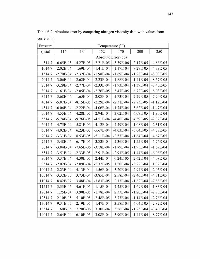
147
Table 6-2. Absolute error by comparing nitrogen viscosity data with values from
correlation
Pressure Temperature (oF) (psia) 116 134 152 170 200 250
Absolute Error (cp) 514.7 -6.65E-05 -4.27E-05 -2.21E-05 -3.39E-06 2.17E-05 4.86E-05
1014.7 -2.02E-04 -1.69E-04 -1.41E-04 -1.17E-04 -8.29E-05 -4.39E-051514.7 -2.70E-04 -2.32E-04 -1.98E-04 -1.69E-04 -1.28E-04 -8.03E-052014.7 -3.06E-04 -2.62E-04 -2.23E-04 -1.88E-04 -1.41E-04 -8.57E-052514.7 -3.29E-04 -2.77E-04 -2.33E-04 -1.93E-04 -1.39E-04 -7.40E-053014.7 -1.61E-04 -2.05E-04 -2.76E-05 3.47E-05 6.72E-05 8.03E-053514.7 -3.68E-04 -1.65E-04 -2.08E-04 1.73E-04 2.29E-05 7.20E-054014.7 -5.87E-04 -8.15E-05 -2.29E-04 -2.31E-04 -2.73E-05 -1.12E-044514.7 -6.06E-04 -2.22E-04 -4.06E-04 -1.74E-04 5.62E-05 -1.47E-045014.7 -4.55E-04 -4.28E-05 -2.94E-04 -3.02E-04 6.07E-05 -1.90E-045514.7 -5.74E-04 -9.76E-05 -4.51E-04 -4.40E-04 4.39E-05 -2.32E-046014.7 -4.75E-04 5.81E-06 -4.12E-04 -4.49E-04 -1.08E-04 -2.31E-046514.7 -4.02E-04 6.23E-05 -5.67E-04 -4.03E-04 -6.04E-05 -4.57E-057014.7 -3.31E-04 8.53E-05 -5.11E-04 -2.53E-04 -1.64E-04 4.67E-057514.7 -3.48E-04 6.17E-05 -3.83E-04 -2.36E-04 -1.55E-04 -5.76E-058014.7 -3.84E-04 -7.65E-06 -3.18E-04 -1.79E-04 -1.95E-04 -1.67E-048514.7 -3.51E-04 -2.33E-05 -2.91E-04 -2.91E-05 -1.44E-04 -6.06E-059014.7 -3.37E-04 -4.30E-05 -2.44E-04 6.24E-05 -2.62E-04 -4.08E-059514.7 -2.02E-04 -2.09E-04 -5.37E-05 1.20E-04 -3.22E-04 1.32E-04
10014.7 -2.23E-04 4.13E-04 -1.56E-04 3.20E-04 -2.94E-04 2.05E-0410514.7 -3.32E-05 3.73E-04 -3.85E-04 2.58E-04 -2.46E-04 -4.71E-0511014.7 8.42E-07 3.48E-04 -3.83E-05 2.13E-04 -1.82E-04 -7.88E-0511514.7 3.33E-06 4.61E-05 -1.15E-04 2.45E-04 -1.69E-04 -1.83E-0412014.7 1.25E-04 3.90E-05 -1.78E-04 2.33E-04 -1.20E-04 -2.73E-0412514.7 2.10E-05 5.10E-05 -2.48E-05 3.73E-04 -1.14E-04 -2.76E-0413014.7 -9.31E-05 2.19E-05 1.47E-04 3.58E-04 -6.04E-05 -2.82E-0413514.7 1.60E-05 7.20E-06 3.30E-04 3.56E-04 -1.25E-04 -3.40E-0414014.7 -2.64E-04 6.10E-05 3.08E-04 3.90E-04 -1.44E-04 -8.77E-05

148
Table 6-2. Continued
Pressure Temperature (oF) (psia) 116 134 152 170 200 250
Absolute Error (cp) 14514.7 -3.11E-04 2.64E-04 3.45E-04 3.46E-04 -1.79E-05 -4.10E-0515014.7 -1.91E-04 1.46E-04 4.48E-04 7.03E-04 -5.72E-05 -6.18E-0515514.7 -2.17E-04 8.17E-05 3.73E-04 6.39E-04 4.28E-05 -2.91E-0416014.7 -3.96E-04 3.08E-05 2.68E-04 6.73E-04 1.89E-04 -4.21E-0416514.7 -3.20E-04 2.95E-05 3.06E-04 7.53E-04 1.65E-04 -5.69E-0417014.7 -2.75E-04 -4.91E-05 2.95E-04 7.73E-04 1.89E-04 -6.83E-0417514.7 -4.30E-04 -1.14E-04 -3.97E-04 8.52E-04 2.91E-04 -6.24E-0418014.7 -4.30E-04 4.33E-06 -1.65E-04 8.77E-04 1.20E-04 -8.39E-0418514.7 -4.63E-04 -3.54E-06 1.75E-04 9.00E-04 2.28E-04 -9.71E-0419014.7 -5.29E-04 4.60E-05 1.37E-04 8.79E-04 2.42E-04 -7.14E-0419514.7 -3.58E-04 -1.37E-04 1.20E-04 8.40E-04 -4.37E-05 -9.24E-0420014.7 -3.77E-04 -1.37E-04 2.81E-04 8.88E-04 7.57E-05 -9.53E-0420514.7 -4.41E-04 -7.32E-05 1.76E-04 9.13E-04 -1.85E-04 -1.42E-0321014.7 -2.61E-04 4.73E-05 2.61E-04 1.05E-03 -7.74E-05 -1.24E-0321514.7 -3.50E-04 -1.61E-04 4.21E-04 1.14E-03 1.24E-04 -1.21E-0322014.7 -5.32E-04 -2.10E-04 4.20E-04 1.23E-03 1.01E-04 -1.20E-0322514.7 -4.98E-04 - 6.68E-04 1.41E-03 1.15E-04 -1.19E-0323014.7 -5.44E-04 - 5.85E-04 1.27E-03 1.45E-04 -1.31E-0323514.7 -3.35E-04 - 6.34E-04 1.48E-03 1.86E-04 -1.23E-0324014.7 - - 5.66E-04 1.35E-03 8.08E-05 - 24514.7 - - - - 2.10E-04 -

149
Table 6-2. Continued
Pressure Temperature (oF) (psia) 260 280 300 330 350 Absolute Error (cp) 514.7 5.18E-05 5.56E-05 5.81E-05 5.50E-05 5.10E-05 1014.7 -3.84E-05 -3.01E-05 -2.54E-05 -2.27E-05 -2.47E-05 1514.7 -7.32E-05 -6.26E-05 -5.53E-05 -4.92E-05 -5.00E-05 2014.7 -7.72E-05 -6.46E-05 -5.44E-05 -4.68E-05 -4.54E-05 2514.7 -6.50E-05 -4.97E-05 -3.78E-05 -2.78E-05 -2.54E-05 3014.7 1.02E-04 8.78E-05 5.03E-05 4.06E-04 7.56E-04 3514.7 5.22E-05 2.48E-06 2.25E-05 1.57E-04 5.89E-04 4014.7 1.53E-05 -1.40E-05 5.08E-05 2.71E-04 1.53E-04 4514.7 8.31E-05 1.58E-04 1.77E-04 3.03E-04 1.05E-04 5014.7 2.03E-04 1.03E-04 6.78E-05 2.62E-04 2.38E-04 5514.7 3.45E-04 8.72E-05 1.48E-04 2.55E-04 2.82E-04 6014.7 4.17E-04 7.86E-05 1.94E-04 2.58E-04 4.26E-04 6514.7 4.79E-04 9.38E-05 1.55E-04 2.66E-04 3.63E-04 7014.7 4.28E-04 9.69E-05 1.40E-04 3.77E-04 3.74E-04 7514.7 3.79E-04 1.21E-04 6.04E-06 3.09E-04 2.86E-04 8014.7 3.15E-04 1.37E-04 1.11E-04 4.15E-04 3.36E-04 8514.7 3.20E-04 8.76E-05 7.18E-05 3.50E-04 3.25E-04 9014.7 3.93E-04 8.07E-05 5.01E-05 1.93E-04 3.20E-04 9514.7 3.08E-04 1.51E-04 6.48E-05 1.08E-04 2.58E-04 10014.7 3.77E-04 8.77E-05 1.03E-04 1.08E-04 1.41E-04 10514.7 3.68E-04 9.53E-05 6.62E-05 1.41E-04 1.04E-04 11014.7 1.82E-04 -4.29E-06 4.96E-05 4.61E-05 1.43E-04 11514.7 4.02E-04 -7.61E-06 2.85E-05 2.18E-04 2.34E-04 12014.7 3.23E-04 -4.13E-05 9.47E-05 5.03E-05 2.02E-04 12514.7 2.15E-04 -6.93E-05 4.66E-05 7.18E-05 1.57E-04 13014.7 2.10E-04 -1.16E-04 1.16E-04 1.03E-04 1.90E-04 13514.7 2.20E-04 -8.61E-05 2.01E-04 8.80E-05 1.45E-04 14014.7 2.42E-04 2.45E-05 5.78E-05 9.47E-05 1.76E-04

150
Table 6-2. Continued
Pressure Temperature (oF) (psia) 260 280 300 330 350 Absolute Error (cp) 14514.7 8.73E-05 2.80E-05 8.25E-05 1.49E-04 9.62E-05 15014.7 1.20E-04 -2.18E-05 1.19E-04 -9.90E-05 1.04E-04 15514.7 1.44E-04 5.20E-05 1.40E-04 -1.60E-05 9.00E-07 16014.7 1.37E-04 -5.29E-06 1.43E-04 4.03E-05 1.15E-04 16514.7 -4.12E-05 -9.39E-05 7.78E-05 5.94E-05 6.04E-05 17014.7 -1.30E-05 -1.36E-04 1.94E-04 1.55E-04 -1.22E-04 17514.7 3.67E-05 -6.81E-05 9.16E-05 2.01E-04 -7.03E-05 18014.7 5.84E-05 -2.01E-04 2.18E-04 -5.90E-05 -1.86E-05 18514.7 -1.44E-05 -2.02E-04 -5.40E-05 -2.22E-04 -9.57E-05 19014.7 -2.06E-04 -1.74E-04 -4.42E-05 -2.93E-04 1.97E-04 19514.7 -3.45E-04 -1.21E-04 5.75E-05 -1.74E-04 -1.12E-05 20014.7 -4.04E-04 -8.78E-05 -2.60E-04 -3.68E-04 3.98E-04 20514.7 -5.25E-04 -9.14E-05 3.31E-05 -1.70E-04 4.08E-04 21014.7 -5.84E-04 -1.35E-04 5.23E-06 -1.76E-04 4.65E-04 21514.7 -6.80E-04 -3.40E-04 1.60E-04 -5.86E-05 1.79E-04 22014.7 -7.02E-04 -4.20E-04 -9.02E-05 -1.45E-04 1.98E-04 22514.7 -7.39E-04 -2.64E-04 -2.11E-04 -2.21E-04 5.59E-05 23014.7 -7.12E-04 -1.69E-04 1.65E-04 -2.22E-04 9.97E-05 23514.7 -6.13E-04 -1.26E-04 1.13E-04 -8.95E-05 1.30E-04 24014.7 -6.05E-04 6.56E-05 2.71E-04 - 1.17E-04 24514.7 -7.44E-04 -3.27E-05 3.54E-04 - -2.60E-04

151
Table 6-3. Relative error by comparing nitrogen viscosity data with values from
correlation
Pressure Temperature (oF) (psia) 116 134 152 170 200 250
Relative Error (%) 514.7 -0.344 -0.216 -0.109 -0.016 0.102 0.217
1014.7 -1.008 -0.830 -0.681 -0.553 -0.380 -0.192 1514.7 -1.301 -1.101 -0.923 -0.773 -0.571 -0.343 2014.7 -1.419 -1.198 -1.004 -0.834 -0.612 -0.357 2514.7 -1.459 -1.216 -1.009 -0.828 -0.582 -0.300 3014.7 -0.689 -0.867 -0.116 0.145 0.276 0.319 3514.7 -1.495 -0.672 -0.837 0.701 0.091 0.278 4014.7 -2.263 -0.319 -0.887 -0.888 -0.104 -0.415 4514.7 -2.238 -0.829 -1.500 -0.646 0.208 -0.530 5014.7 -1.623 -0.155 -1.053 -1.077 0.218 -0.666 5514.7 -1.959 -0.339 -1.548 -1.507 0.153 -0.789 6014.7 -1.563 0.020 -1.367 -1.489 -0.362 -0.762 6514.7 -1.278 0.202 -1.810 -1.294 -0.196 -0.148 7014.7 -1.017 0.268 -1.581 -0.793 -0.516 0.148 7514.7 -1.032 0.187 -1.152 -0.717 -0.475 -0.177 8014.7 -1.102 -0.022 -0.930 -0.527 -0.580 -0.500 8514.7 -0.975 -0.066 -0.827 -0.084 -0.417 -0.177 9014.7 -0.910 -0.118 -0.675 0.175 -0.737 -0.116 9514.7 -0.532 -0.557 -0.145 0.329 -0.882 0.369
10014.7 -0.568 1.087 -0.409 0.859 -0.787 0.564 10514.7 -0.083 0.955 -0.977 0.674 -0.643 -0.126 11014.7 0.002 0.867 -0.096 0.543 -0.466 -0.206 11514.7 0.008 0.111 -0.279 0.610 -0.424 -0.466 12014.7 0.290 0.092 -0.424 0.566 -0.294 -0.681 12514.7 0.047 0.117 -0.058 0.890 -0.274 -0.677 13014.7 -0.205 0.049 0.337 0.836 -0.142 -0.677 13514.7 0.035 0.016 0.742 0.814 -0.289 -0.800 14014.7 -0.554 0.131 0.680 0.875 -0.325 -0.204

152
Table 6-3. Continued
Pressure Temperature (oF) (psia) 116 134 152 170 200 250
Relative Error (%) 14514.7 -0.640 0.561 0.746 0.759 -0.040 -0.094 15014.7 -0.385 0.303 0.951 1.525 -0.125 -0.139 15514.7 -0.428 0.166 0.776 1.358 0.092 -0.640 16014.7 -0.766 0.061 0.546 1.406 0.401 -0.909 16514.7 -0.607 0.058 0.612 1.549 0.344 -1.205 17014.7 -0.513 -0.094 0.580 1.563 0.387 -1.421 17514.7 -0.785 -0.214 -0.757 1.695 0.588 -1.280 18014.7 -0.772 0.008 -0.311 1.717 0.238 -1.687 18514.7 -0.816 -0.006 0.326 1.734 0.446 -1.921 19014.7 -0.916 0.082 0.251 1.666 0.465 -1.399 19514.7 -0.612 -0.242 0.217 1.566 -0.082 -1.779 20014.7 -0.634 -0.236 0.501 1.631 0.141 -1.809 20514.7 -0.730 -0.125 0.308 1.653 -0.338 -2.631 21014.7 -0.427 0.080 0.450 1.874 -0.140 -2.283 21514.7 -0.563 -0.266 0.720 2.010 0.221 -2.190 22014.7 -0.840 -0.341 0.706 2.152 0.178 -2.146 22514.7 -0.775 - 1.113 2.436 0.200 -2.113 23014.7 -0.834 - 0.961 2.156 0.249 -2.287 23514.7 -0.509 - 1.027 2.489 0.316 -2.129 24014.7 - - 0.904 2.238 0.135 - 24514.7 - - - - 0.347 -

153
Table 6-3. Continued
Pressure Temperature (oF) (psia) 260 280 300 330 350 Relative Error (%) 514.7 0.229 0.241 0.247 0.228 0.208 1014.7 -0.166 -0.128 -0.106 -0.092 -0.099 1514.7 -0.310 -0.261 -0.226 -0.196 -0.197 2014.7 -0.319 -0.263 -0.218 -0.184 -0.175 2514.7 -0.262 -0.197 -0.148 -0.107 -0.096 3014.7 0.404 0.342 0.193 1.551 2.886 3514.7 0.200 0.009 0.084 0.578 2.185 4014.7 0.057 -0.051 0.185 0.981 0.547 4514.7 0.301 0.568 0.631 1.073 0.367 5014.7 0.719 0.361 0.235 0.902 0.813 5514.7 1.194 0.297 0.503 0.857 0.942 6014.7 1.404 0.261 0.642 0.850 1.400 6514.7 1.577 0.304 0.501 0.857 1.165 7014.7 1.367 0.306 0.441 1.191 1.174 7514.7 1.180 0.373 0.019 0.952 0.878 8014.7 0.955 0.412 0.333 1.255 1.009 8514.7 0.948 0.257 0.211 1.033 0.958 9014.7 1.136 0.232 0.144 0.556 0.923 9514.7 0.869 0.425 0.182 0.304 0.730 10014.7 1.042 0.241 0.284 0.297 0.391 10514.7 0.995 0.257 0.179 0.382 0.281 11014.7 0.479 -0.011 0.131 0.122 0.381 11514.7 1.045 -0.020 0.074 0.571 0.615 12014.7 0.822 -0.104 0.242 0.129 0.519 12514.7 0.535 -0.172 0.117 0.181 0.396 13014.7 0.512 -0.282 0.285 0.256 0.474 13514.7 0.526 -0.206 0.487 0.214 0.356 14014.7 0.570 0.058 0.137 0.227 0.424

154
Table 6-3. Continued
Pressure Temperature (oF) (psia) 260 280 300 330 350 Relative Error (%) 14514.7 0.201 0.065 0.193 0.352 0.228 15014.7 0.272 -0.050 0.273 -0.229 0.242 15514.7 0.321 0.117 0.317 -0.037 0.002 16014.7 0.301 -0.012 0.320 0.091 0.260 16514.7 -0.089 -0.204 0.171 0.132 0.135 17014.7 -0.028 -0.291 0.420 0.340 -0.266 17514.7 0.077 -0.144 0.196 0.435 -0.152 18014.7 0.120 -0.416 0.460 -0.125 -0.040 18514.7 -0.029 -0.413 -0.112 -0.464 -0.202 19014.7 -0.410 -0.350 -0.090 -0.603 0.412 19514.7 -0.676 -0.241 0.116 -0.353 -0.023 20014.7 -0.780 -0.173 -0.515 -0.737 0.815 20514.7 -0.997 -0.177 0.065 -0.338 0.827 21014.7 -1.095 -0.259 0.010 -0.346 0.933 21514.7 -1.256 -0.641 0.308 -0.114 0.352 22014.7 -1.280 -0.781 -0.170 -0.279 0.385 22514.7 -1.329 -0.485 -0.393 -0.417 0.107 23014.7 -1.267 -0.307 0.307 -0.416 0.190 23514.7 -1.079 -0.227 0.206 -0.166 0.244 24014.7 -1.053 0.117 0.493 - 0.218 24514.7 -1.278 -0.058 0.637 - -0.476
6.2 Methane Viscosity Correlation
Since Lee-Gonzalez-Eakin correlation is one of the most common used viscosity
correlations in petroleum engineering and can be coded into computer program easily, we
developed a correlation that has the same form as Lee-Gonzalez-Eakin correlation. The
coefficients in the correlation were updated using NIST values and lab data from our
experiment. Due to the fact that we do not have viscosity data at pressure from 500 to
4500 psi in our experiment, NIST values at this pressure range were used. As we already
showed in Chapter II, NIST values match with lab data very well at pressure from 500 to
4500 psi. Combining NIST values at pressure from 514.7 to 4014.7 psia with our lab data
at pressure from 4514.7 to 24514.7 psia the coefficients were determined. A non-linear

155
regression approach is applied in determining the coefficients. As a result, the final form
of correlation was developed. New gas viscosity correlation is as follows:
( )Ygg XK ρμ exp= . (6.5)
where
TM
TMK
w
w++
+=
83933.1899.208
)0893.318999.9(*0001.0 2288.1
. (6.6)
wMT
X 124465.001.1000
56014.3 ++= ⎥⎦⎤
⎢⎣⎡ . (6.7)
XY 12294.047862.2 −= . (6.8)
where
gμ = Gas viscosity, cp
gρ = Gas density, g/cc
MW = Molecular weight
T = Temperature, R
New correlation that based on lab data and NIST values (Table 6-3) covers larger
pressure and temperature range than original Lee-Gonzalez-Eakin correlation. It covers
both low and high pressure and temperature and gives more confidence on gas viscosity
estimation when petroleum engineers deal with HPHT reservoir.

156
Table 6-4. Data used to develop new methane viscosity correlation
Pressure Temperature (oF) (psia) 100 120 140 160 180 514.7 0.01216 0.01248 0.01280 0.01312 0.01343 1014.7 0.01303 0.01328 0.01355 0.01382 0.01409 1514.7 0.01420 0.01436 0.01453 0.01473 0.01494 2014.7 0.01568 0.01568 0.01573 0.01583 0.01595 2514.7 0.01739 0.01720 0.01711 0.01708 0.01709 3014.7 0.01921 0.01884 0.01859 0.01843 0.01834 3514.7 0.02105 0.02052 0.02013 0.01984 0.01964 4014.7 0.02284 0.02218 0.02166 0.02126 0.02095 4514.7 0.02454 0.02377 0.02309 0.02265 0.02226 5014.7 0.02630 0.02531 0.02447 0.02399 0.02376 5514.7 0.02772 0.02675 0.02547 0.02517 0.02490 6014.7 0.02977 0.02790 0.02678 0.02628 0.02599 6514.7 0.03082 0.02886 0.02836 0.02746 0.02707 7014.7 0.03156 0.02995 0.02959 0.02854 0.02806 7514.7 0.03298 0.03108 0.03093 0.02968 0.02900 8014.7 0.03413 0.03224 0.03200 0.03027 0.03018 8514.7 0.03529 0.03344 0.03314 0.03124 0.03110 9014.7 0.03656 0.03470 0.03421 0.03232 0.03195 9514.7 0.03772 0.03585 0.03523 0.03349 0.03279 10014.7 0.03879 0.03700 0.03620 0.03446 0.03376 10514.7 0.03989 0.03807 0.03726 0.03548 0.03484 11014.7 0.04101 0.03915 0.03813 0.03647 0.03552 11514.7 0.04205 0.04020 0.03896 0.03739 0.03643 12014.7 0.04305 0.04118 0.03986 0.03837 0.03732 12514.7 0.04401 0.04218 0.04079 0.03931 0.03825 13014.7 0.04505 0.04311 0.04182 0.04022 0.03916 13514.7 0.04609 0.04412 0.04270 0.04113 0.04005 14014.7 0.04714 0.04512 0.04369 0.04210 0.04088 14514.7 0.04822 0.04614 0.04461 0.04304 0.04179 15014.7 0.04915 0.04709 0.04558 0.04388 0.04272 15514.7 0.05020 0.04812 0.04654 0.04467 0.04361 16014.7 0.05126 0.04901 0.04743 0.04586 0.04443 16514.7 0.05220 0.05004 0.04834 0.04690 0.04530 17014.7 0.05323 0.05106 0.04926 0.04776 0.04612 17514.7 0.05428 0.05204 0.05015 0.04856 0.04708 18014.7 0.05533 0.05303 0.05112 0.04955 0.04799

157
Table 6-4. Continued
Pressure Temperature (oF) (psia) 100 120 140 160 180
18514.7 0.05636 0.05393 0.05204 0.05047 0.04881 19014.7 0.05743 0.05490 0.05284 0.05123 0.04966 19514.7 0.05836 0.05588 0.05378 0.05217 0.05056 20014.7 0.05937 0.05693 0.05474 0.05302 0.05138 20514.7 0.06041 0.05789 0.05556 0.05391 0.05220 21014.7 0.06187 0.05888 0.05657 0.05479 0.05306 21514.7 0.06257 0.05993 0.05744 0.05567 0.05391 22014.7 0.06355 0.06096 0.05839 0.05656 0.05481 22514.7 0.06461 0.06220 0.05931 0.05753 0.05566 23014.7 0.06575 0.06277 0.06017 0.05837 0.05650 23514.7 0.06683 0.06402 0.06116 0.05914 0.05719 24014.7 0.06777 0.06505 0.06209 0.05975 0.05819 24514.7 0.06893 0.06603 0.06301 0.06064 0.05915 25014.7 0.07002 - 0.06389 0.06173 0.06007
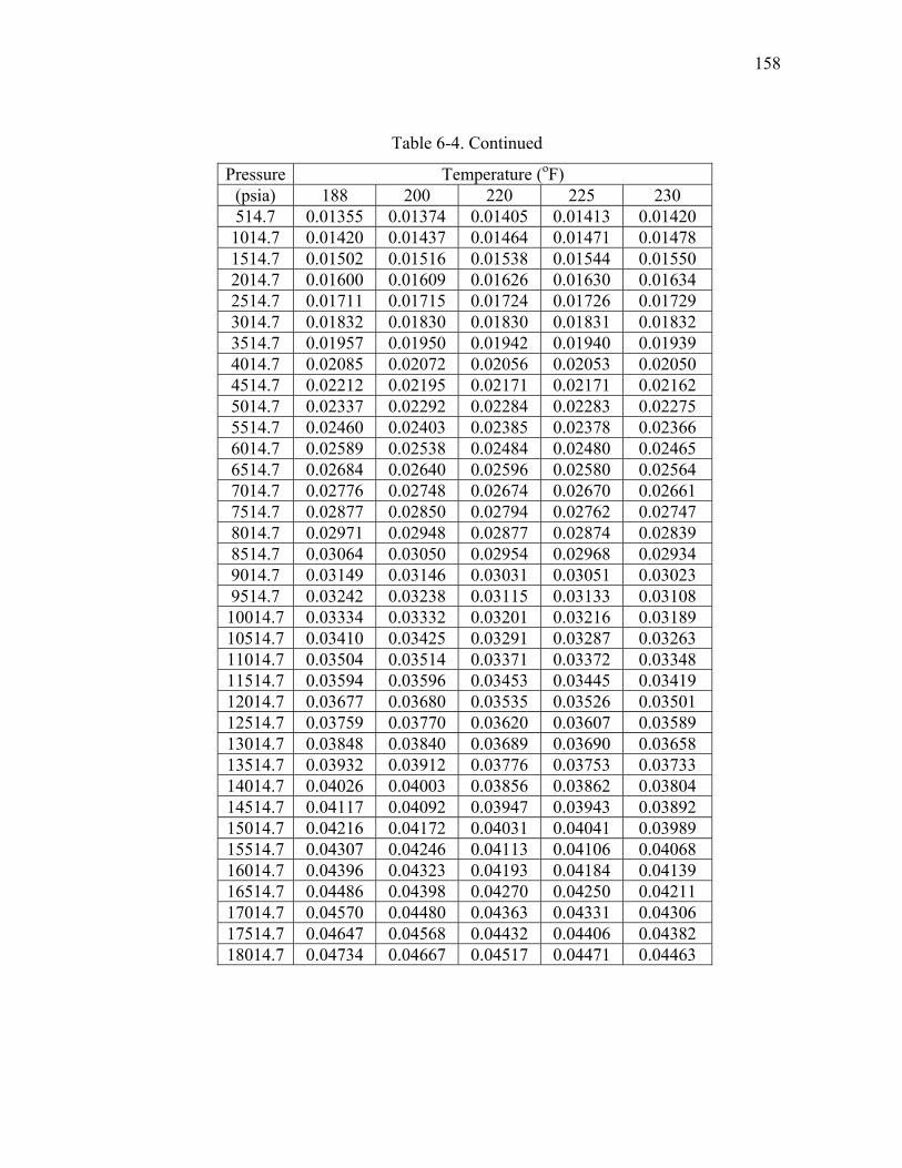
158
Table 6-4. Continued
Pressure Temperature (oF) (psia) 188 200 220 225 230 514.7 0.01355 0.01374 0.01405 0.01413 0.01420 1014.7 0.01420 0.01437 0.01464 0.01471 0.01478 1514.7 0.01502 0.01516 0.01538 0.01544 0.01550 2014.7 0.01600 0.01609 0.01626 0.01630 0.01634 2514.7 0.01711 0.01715 0.01724 0.01726 0.01729 3014.7 0.01832 0.01830 0.01830 0.01831 0.01832 3514.7 0.01957 0.01950 0.01942 0.01940 0.01939 4014.7 0.02085 0.02072 0.02056 0.02053 0.02050 4514.7 0.02212 0.02195 0.02171 0.02171 0.02162 5014.7 0.02337 0.02292 0.02284 0.02283 0.02275 5514.7 0.02460 0.02403 0.02385 0.02378 0.02366 6014.7 0.02589 0.02538 0.02484 0.02480 0.02465 6514.7 0.02684 0.02640 0.02596 0.02580 0.02564 7014.7 0.02776 0.02748 0.02674 0.02670 0.02661 7514.7 0.02877 0.02850 0.02794 0.02762 0.02747 8014.7 0.02971 0.02948 0.02877 0.02874 0.02839 8514.7 0.03064 0.03050 0.02954 0.02968 0.02934 9014.7 0.03149 0.03146 0.03031 0.03051 0.03023 9514.7 0.03242 0.03238 0.03115 0.03133 0.03108 10014.7 0.03334 0.03332 0.03201 0.03216 0.03189 10514.7 0.03410 0.03425 0.03291 0.03287 0.03263 11014.7 0.03504 0.03514 0.03371 0.03372 0.03348 11514.7 0.03594 0.03596 0.03453 0.03445 0.03419 12014.7 0.03677 0.03680 0.03535 0.03526 0.03501 12514.7 0.03759 0.03770 0.03620 0.03607 0.03589 13014.7 0.03848 0.03840 0.03689 0.03690 0.03658 13514.7 0.03932 0.03912 0.03776 0.03753 0.03733 14014.7 0.04026 0.04003 0.03856 0.03862 0.03804 14514.7 0.04117 0.04092 0.03947 0.03943 0.03892 15014.7 0.04216 0.04172 0.04031 0.04041 0.03989 15514.7 0.04307 0.04246 0.04113 0.04106 0.04068 16014.7 0.04396 0.04323 0.04193 0.04184 0.04139 16514.7 0.04486 0.04398 0.04270 0.04250 0.04211 17014.7 0.04570 0.04480 0.04363 0.04331 0.04306 17514.7 0.04647 0.04568 0.04432 0.04406 0.04382 18014.7 0.04734 0.04667 0.04517 0.04471 0.04463

159
Table 6-4. Continued
Pressure Temperature (oF) (psia) 188 200 220 225 230
18514.7 0.04821 0.04773 0.04586 0.04561 0.04537 19014.7 0.04907 0.04840 0.04661 0.04642 0.04619 19514.7 0.04995 0.04919 0.04725 0.04724 0.04691 20014.7 0.05088 0.05013 0.04789 0.04804 0.04773 20514.7 0.05136 0.05092 0.04872 0.04879 0.04858 21014.7 0.05210 0.05188 0.04949 0.04951 0.04935 21514.7 0.05296 0.05270 0.05039 0.05036 0.05010 22014.7 0.05377 0.05347 0.05116 0.05115 0.05086 22514.7 0.05460 0.05418 0.05199 0.05191 0.05166 23014.7 0.05550 0.05503 0.05282 0.05280 0.05243 23514.7 0.05637 0.05584 0.05369 0.05365 0.05321 24014.7 0.05726 0.05650 0.05416 0.05442 0.05394 24514.7 0.05795 0.05731 0.05494 0.05522 0.05454 25014.7 - - 0.05587 0.05608 -

160
Table 6-4. Continued
Pressure Temperature (oF) (psia) 250 260 280 300 320 514.7 0.01451 0.01466 0.01496 0.01526 0.01555 1014.7 0.01506 0.01519 0.01547 0.01574 0.01602 1514.7 0.01573 0.01585 0.01609 0.01634 0.01658 2014.7 0.01652 0.01662 0.01682 0.01702 0.01723 2514.7 0.01741 0.01748 0.01762 0.01778 0.01795 3014.7 0.01837 0.01840 0.01849 0.01860 0.01872 3514.7 0.01938 0.01938 0.01941 0.01947 0.01954 4014.7 0.02041 0.02039 0.02036 0.02036 0.02039 4514.7 0.02147 0.02140 0.02132 0.02126 0.02124 5014.7 0.02239 0.02238 0.02221 0.02208 0.02191 5514.7 0.02333 0.02334 0.02315 0.02294 0.02272 6014.7 0.02426 0.02427 0.02405 0.02376 0.02356 6514.7 0.02516 0.02520 0.02499 0.02466 0.02443 7014.7 0.02611 0.02602 0.02586 0.02546 0.02524 7514.7 0.02704 0.02692 0.02670 0.02624 0.02604 8014.7 0.02794 0.02791 0.02758 0.02705 0.02679 8514.7 0.02882 0.02873 0.02844 0.02776 0.02754 9014.7 0.02959 0.02961 0.02928 0.02866 0.02834 9514.7 0.03046 0.03041 0.03002 0.02943 0.02908 10014.7 0.03126 0.03118 0.03083 0.03022 0.02982 10514.7 0.03205 0.03194 0.03157 0.03094 0.03065 11014.7 0.03287 0.03269 0.03237 0.03165 0.03141 11514.7 0.03375 0.03338 0.03320 0.03241 0.03212 12014.7 0.03455 0.03429 0.03399 0.03353 0.03283 12514.7 0.03537 0.03504 0.03479 0.03438 0.03354 13014.7 0.03614 0.03586 0.03556 0.03508 0.03425 13514.7 0.03676 0.03666 0.03632 0.03584 0.03501 14014.7 0.03752 0.03739 0.03714 0.03659 0.03575 14514.7 0.03835 0.03827 0.03792 0.03725 0.03651 15014.7 0.03932 0.03906 0.03885 0.03805 0.03727 15514.7 0.03998 0.03988 0.03949 0.03882 0.03810 16014.7 0.04084 0.04051 0.04035 0.03961 0.03885 16514.7 0.04148 0.04127 0.04105 0.04048 0.03964 17014.7 0.04222 0.04194 0.04193 0.04115 0.04048 17514.7 0.04294 0.04281 0.04259 0.04196 0.04115 18014.7 0.04365 0.04357 0.04336 0.04275 0.04189

161
Table 6-4. Continued
Pressure Temperature (oF) (psia) 250 260 280 300 320
18514.7 0.04437 0.04445 0.04407 0.04336 0.04282 19014.7 0.04514 0.04521 0.04480 0.04414 0.04350 19514.7 0.04593 0.04609 0.04559 0.04491 0.04408 20014.7 0.04665 0.04681 0.04622 0.04564 0.04476 20514.7 0.04757 0.04759 0.04702 0.04646 0.04544 21014.7 0.04842 0.04847 0.04786 0.04708 0.04606 21514.7 0.04932 0.04915 0.04849 0.04791 0.04686 22014.7 0.05008 0.04996 0.04915 0.04868 0.04759 22514.7 0.05083 0.05080 0.04987 0.04928 0.04836 23014.7 0.05141 0.05165 0.05060 0.05005 0.04894 23514.7 0.05204 0.05226 0.05132 0.05071 0.04976 24014.7 0.05294 0.05263 0.05195 0.05156 0.05083 24514.7 0.05357 0.05335 0.05263 0.05200 0.05155 25014.7 - 0.05407 0.05337 - 0.05228

162
Table 6-4. Continued
Pressure Temperature (oF) (psia) 340 360 380 415 514.7 0.01584 0.01613 0.01642 0.01691 1014.7 0.01629 0.01656 0.01683 0.01730 1514.7 0.01683 0.01708 0.01732 0.01776 2014.7 0.01745 0.01766 0.01789 0.01828 2514.7 0.01813 0.01831 0.01850 0.01885 3014.7 0.01886 0.01901 0.01917 0.01946 3514.7 0.01964 0.01974 0.01987 0.02010 4014.7 0.02044 0.02050 0.02059 0.02077 4514.7 0.02096 0.02128 0.02133 0.02147 5014.7 0.02181 0.02206 0.02205 0.02217 5514.7 0.02283 0.02284 0.02278 0.02284 6014.7 0.02369 0.02366 0.02361 0.02353 6514.7 0.02443 0.02435 0.02424 0.02429 7014.7 0.02512 0.02500 0.02494 0.02496 7514.7 0.02585 0.02578 0.02565 0.02564 8014.7 0.02665 0.02641 0.02637 0.02635 8514.7 0.02748 0.02740 0.02714 0.02697 9014.7 0.02841 0.02817 0.02786 0.02764 9514.7 0.02908 0.02886 0.02859 0.02827 10014.7 0.02980 0.02954 0.02922 0.02892 10514.7 0.03058 0.03032 0.02995 0.02957 11014.7 0.03133 0.03110 0.03054 0.03028 11514.7 0.03202 0.03178 0.03123 0.03083 12014.7 0.03279 0.03243 0.03194 0.03145 12514.7 0.03356 0.03306 0.03261 0.03214 13014.7 0.03432 0.03378 0.03333 0.03280 13514.7 0.03501 0.03437 0.03400 0.03346 14014.7 0.03577 0.03503 0.03467 0.03411 14514.7 0.03650 0.03568 0.03530 0.03472 15014.7 0.03720 0.03639 0.03599 0.03531 15514.7 0.03804 0.03708 0.03661 0.03577 16014.7 0.03912 0.03780 0.03730 0.03642 16514.7 0.03971 0.03849 0.03797 0.03698 17014.7 0.04039 0.03918 0.03866 0.03767 17514.7 0.04099 0.03986 0.03934 0.03830 18014.7 0.04203 0.04057 0.04000 0.03915

163
Table 6-4. Continued
Pressure Temperature (oF) (psia) 340 360 380 415
18514.7 0.04272 0.04138 0.04068 0.03965 19014.7 0.04339 0.04184 0.04132 0.04041 19514.7 0.04404 0.04255 0.04194 0.04088 20014.7 0.04458 0.04325 0.04254 0.04145 20514.7 0.04526 0.04391 0.04323 0.04214 21014.7 0.04588 0.04420 0.04380 0.04257 21514.7 0.04658 0.04486 0.04431 0.04303 22014.7 0.04711 0.04544 0.04502 0.04380 22514.7 0.04788 0.04599 0.04570 0.04420 23014.7 0.04836 0.04653 0.04628 0.04465 23514.7 0.04891 0.04717 0.04677 0.04531 24014.7 0.04939 0.04778 0.04740 0.04559 24514.7 0.05011 0.04895 0.04796 0.04620 25014.7 0.05071 - 0.04866 -
The accuracy of the new methane correlation is vital for future viscosity estimation. As
well as error analysis for nitrogen viscosity we compared the calculated viscosity from
correlation with lab data. In analysis lab data are used as base for both absolute error and
relative error. Tables 6-5 and 6-6 show the absolute error and relative error. Average
absolute error is 7.06E-06 cp. Average relative error is 0.1068%.

164
Table 6-5. Absolute error by comparing methane viscosity data with values from
correlation
Pressure Temperature (oF) (psia) 100 120 140 160 180 188 200
Absolute Error (cp) 514.7 1.17E-03 1.15E-03 1.13E-03 1.11E-03 1.09E-03 1.08E-03 1.06E-031014.7 8.66E-04 8.62E-04 8.55E-04 8.46E-04 8.32E-04 8.26E-04 8.16E-041514.7 5.58E-04 5.70E-04 5.78E-04 5.81E-04 5.79E-04 5.78E-04 5.74E-042014.7 2.54E-04 2.82E-04 3.05E-04 3.21E-04 3.33E-04 3.36E-04 3.39E-042514.7 -2.69E-05 1.34E-05 4.80E-05 7.67E-05 1.00E-04 1.07E-04 1.17E-043014.7 -2.62E-04 -2.19E-04 -1.79E-04 -1.42E-04 -1.11E-04 -9.95E-05 -8.44E-053514.7 -4.42E-04 -4.03E-04 -3.65E-04 -3.26E-04 -2.91E-04 -2.78E-04 -2.60E-044014.7 -5.62E-04 -5.39E-04 -5.05E-04 -4.71E-04 -4.35E-04 -4.23E-04 -4.03E-044514.7 -6.27E-04 -6.24E-04 -5.40E-04 -5.75E-04 -5.44E-04 -5.34E-04 -5.14E-045014.7 -8.10E-04 -6.85E-04 -5.44E-04 -6.22E-04 -8.46E-04 -6.09E-04 -3.66E-045514.7 -6.97E-04 -6.82E-04 -1.87E-04 -5.27E-04 -7.87E-04 -6.72E-04 -3.54E-046014.7 -1.28E-03 -4.42E-04 -1.78E-04 -3.95E-04 -7.00E-04 -8.03E-04 -5.77E-046514.7 -9.14E-04 -4.59E-05 -4.71E-04 -3.49E-04 -6.15E-04 -6.20E-04 -4.99E-047014.7 -2.79E-04 1.76E-04 -4.49E-04 -2.31E-04 -4.63E-04 -4.23E-04 -4.92E-047514.7 -3.70E-04 3.26E-04 -5.63E-04 -2.04E-04 -2.91E-04 -3.35E-04 -4.43E-048014.7 -2.28E-04 4.04E-04 -4.48E-04 3.48E-04 -3.77E-04 -1.90E-04 -3.68E-048514.7 -1.34E-04 4.14E-04 -4.22E-04 4.93E-04 -2.20E-04 -6.91E-05 -3.61E-049014.7 -1.78E-04 3.28E-04 -3.58E-04 5.09E-04 -1.32E-05 1.19E-04 -3.10E-049514.7 -1.48E-04 3.30E-04 -2.67E-04 4.11E-04 1.78E-04 2.06E-04 -2.34E-0410014.7 -5.87E-05 2.98E-04 -1.54E-04 4.83E-04 2.18E-04 2.90E-04 -1.90E-0410514.7 -2.04E-05 3.29E-04 -1.42E-04 4.98E-04 1.38E-04 5.06E-04 -1.56E-0411014.7 -1.16E-05 3.36E-04 3.36E-05 5.17E-04 4.33E-04 5.40E-04 -9.99E-0511514.7 4.35E-05 3.46E-04 2.23E-04 5.99E-04 4.85E-04 5.93E-04 1.73E-0512014.7 1.15E-04 4.12E-04 3.33E-04 5.99E-04 5.54E-04 6.94E-04 1.00E-0412514.7 2.21E-04 4.37E-04 4.01E-04 6.18E-04 5.57E-04 8.02E-04 1.06E-0413014.7 2.26E-04 5.25E-04 3.57E-04 6.57E-04 5.69E-04 8.24E-04 3.03E-0413514.7 2.24E-04 5.15E-04 4.44E-04 6.86E-04 5.96E-04 8.80E-04 4.64E-0414014.7 1.83E-04 4.96E-04 4.14E-04 6.47E-04 6.55E-04 8.35E-04 4.31E-04

165
Table 6-5. Continued
Pressure Temperature (oF) (psia) 100 120 140 160 180 188 200
Absolute Error (cp) 14514.7 1.16E-04 4.51E-04 4.30E-04 6.19E-04 6.36E-04 7.99E-04 4.09E-0415014.7 1.70E-04 4.57E-04 3.99E-04 6.85E-04 5.85E-04 6.77E-04 4.61E-0415514.7 1.10E-04 3.83E-04 3.58E-04 7.98E-04 5.66E-04 6.33E-04 5.67E-0416014.7 1.95E-05 4.29E-04 3.82E-04 4.90E-04 6.13E-04 5.96E-04 6.29E-0416514.7 4.19E-05 3.26E-04 3.70E-04 3.26E-04 5.90E-04 5.40E-04 7.09E-0417014.7 -4.41E-05 2.39E-04 3.49E-04 3.31E-04 6.11E-04 5.29E-04 7.09E-0417514.7 -1.49E-04 1.60E-04 3.42E-04 3.88E-04 4.88E-04 5.94E-04 6.47E-0418014.7 -2.71E-04 8.15E-05 2.50E-04 2.58E-04 4.12E-04 5.41E-04 4.62E-0418514.7 -3.76E-04 8.14E-05 2.02E-04 1.82E-04 4.14E-04 4.86E-04 2.02E-0419014.7 -5.18E-04 3.78E-06 2.68E-04 2.66E-04 3.84E-04 4.39E-04 3.28E-0419514.7 -5.39E-04 -9.61E-05 1.83E-04 1.58E-04 2.92E-04 3.52E-04 3.30E-0420014.7 -6.42E-04 -2.67E-04 7.26E-05 1.37E-04 2.75E-04 2.20E-04 1.74E-0420514.7 -7.86E-04 -3.61E-04 1.05E-04 6.20E-05 2.60E-04 5.35E-04 1.65E-0421014.7 -1.34E-03 -4.86E-04 -7.12E-05 1.78E-06 1.87E-04 5.76E-04 -2.98E-0521514.7 -1.16E-03 -6.64E-04 -9.99E-05 -7.26E-05 1.31E-04 5.06E-04 -7.47E-0522014.7 -1.26E-03 -8.45E-04 -2.25E-04 -1.48E-04 1.26E-05 4.63E-04 -7.71E-0522514.7 -1.44E-03 -1.23E-03 -3.19E-04 -3.18E-04 -5.20E-05 4.07E-04 -3.23E-0523014.7 -1.71E-03 -9.58E-04 -3.64E-04 -3.60E-04 -1.14E-04 2.76E-04 -1.22E-0423514.7 -1.92E-03 -1.37E-03 -5.35E-04 -3.36E-04 -3.81E-05 1.63E-04 -1.78E-0424014.7 -1.99E-03 -1.56E-03 -6.48E-04 -1.53E-04 -2.66E-04 3.45E-05 -1.00E-0424514.7 -2.29E-03 -1.70E-03 -7.66E-04 -2.64E-04 -4.68E-04 9.71E-05 -1.63E-0425014.7 -2.53E-03 - -8.40E-04 -5.70E-04 -6.23E-04 - -

166
Table 6-5. Continued
Pressure Temperature (oF) (psia) 220 225 230 250 260 280 Absolute Error (cp)
514.7 1.04E-03 1.03E-03 1.02E-03 9.91E-04 9.74E-04 9.40E-041014.7 7.97E-04 7.92E-04 7.87E-04 7.64E-04 7.51E-04 7.25E-041514.7 5.65E-04 5.63E-04 5.60E-04 5.45E-04 5.37E-04 5.18E-042014.7 3.41E-04 3.41E-04 3.40E-04 3.37E-04 3.32E-04 3.22E-042514.7 1.29E-04 1.32E-04 1.34E-04 1.39E-04 1.40E-04 1.39E-043014.7 -6.32E-05 -5.93E-05 -5.57E-05 -4.20E-05 -3.72E-05 -3.14E-053514.7 -2.33E-04 -2.27E-04 -2.22E-04 -2.02E-04 -1.95E-04 -1.83E-044014.7 -3.74E-04 -3.68E-04 -3.62E-04 -3.39E-04 -3.29E-04 -3.13E-044514.7 -4.87E-04 -5.33E-04 -4.78E-04 -4.55E-04 -4.37E-04 -4.20E-045014.7 -5.66E-04 -6.11E-04 -5.87E-04 -4.21E-04 -4.84E-04 -4.40E-045514.7 -5.13E-04 -5.19E-04 -4.77E-04 -3.88E-04 -5.02E-04 -4.87E-046014.7 -4.54E-04 -4.99E-04 -4.36E-04 -3.45E-04 -4.83E-04 -4.84E-046514.7 -5.19E-04 -4.69E-04 -4.01E-04 -2.75E-04 -4.67E-04 -5.24E-047014.7 -2.61E-04 -3.35E-04 -3.62E-04 -2.64E-04 -3.48E-04 -4.91E-047514.7 -4.38E-04 -2.50E-04 -2.18E-04 -2.33E-04 -3.08E-04 -4.42E-048014.7 -2.61E-04 -3.72E-04 -1.53E-04 -1.87E-04 -3.71E-04 -4.33E-048514.7 -4.19E-05 -3.28E-04 -1.31E-04 -1.36E-04 -2.73E-04 -4.09E-049014.7 1.61E-04 -1.98E-04 -6.06E-05 2.32E-05 -2.46E-04 -3.76E-049514.7 2.80E-04 -5.63E-05 3.43E-05 5.85E-05 -1.53E-04 -2.46E-04
10014.7 3.69E-04 4.99E-05 1.45E-04 1.61E-04 -4.19E-05 -2.07E-0410514.7 4.00E-04 2.66E-04 3.27E-04 2.56E-04 6.40E-05 -9.99E-0511014.7 5.16E-04 3.19E-04 3.83E-04 3.09E-04 1.79E-04 -6.89E-0511514.7 6.09E-04 4.87E-04 5.63E-04 2.99E-04 3.43E-04 -7.75E-0512014.7 6.81E-04 5.65E-04 6.26E-04 3.49E-04 2.70E-04 -5.01E-0512514.7 7.06E-04 6.35E-04 6.08E-04 3.66E-04 3.49E-04 -4.29E-0513014.7 8.88E-04 6.64E-04 7.76E-04 4.31E-04 3.53E-04 -1.16E-0513514.7 8.84E-04 8.88E-04 8.74E-04 6.39E-04 3.65E-04 1.52E-0514014.7 9.26E-04 6.35E-04 1.01E-03 6.94E-04 4.39E-04 -1.95E-05

167
Table 6-5. Continued
Pressure Temperature (oF) (psia) 220 225 230 250 260 280 Absolute Error (cp) 14514.7 8.59E-04 6.62E-04 9.50E-04 6.68E-04 3.60E-04 -2.23E-0515014.7 8.51E-04 5.13E-04 8.02E-04 5.01E-04 3.51E-04 -1.89E-0415514.7 8.50E-04 6.79E-04 8.21E-04 6.34E-04 3.16E-04 -6.35E-0516014.7 8.63E-04 7.10E-04 9.18E-04 5.46E-04 4.54E-04 -1.73E-0416514.7 9.07E-04 8.54E-04 9.91E-04 6.88E-04 4.65E-04 -1.27E-0417014.7 7.78E-04 8.41E-04 8.34E-04 7.22E-04 5.51E-04 -2.62E-0417514.7 8.85E-04 8.75E-04 8.58E-04 7.61E-04 4.36E-04 -1.87E-0418014.7 8.15E-04 1.00E-03 8.26E-04 8.11E-04 4.23E-04 -2.30E-0418514.7 9.02E-04 8.84E-04 8.54E-04 8.43E-04 2.93E-04 -2.11E-0419014.7 9.27E-04 8.45E-04 7.97E-04 8.21E-04 2.67E-04 -2.19E-0419514.7 1.06E-03 7.93E-04 8.32E-04 7.69E-04 1.25E-04 -2.98E-0420014.7 1.19E-03 7.49E-04 7.75E-04 7.87E-04 1.29E-04 -2.17E-0420514.7 1.12E-03 7.57E-04 6.78E-04 5.98E-04 7.28E-05 -3.11E-0421014.7 1.10E-03 7.81E-04 6.50E-04 4.77E-04 -9.07E-05 -4.48E-0421514.7 9.46E-04 6.72E-04 6.34E-04 2.94E-04 -6.26E-05 -3.77E-0422014.7 9.25E-04 6.25E-04 6.16E-04 2.52E-04 -1.62E-04 -3.48E-0422514.7 8.33E-04 6.03E-04 5.48E-04 2.19E-04 -2.84E-04 -3.77E-0423014.7 7.37E-04 4.44E-04 5.11E-04 3.50E-04 -4.36E-04 -4.12E-0423514.7 6.04E-04 3.28E-04 4.47E-04 4.26E-04 -3.50E-04 -4.52E-0424014.7 8.64E-04 2.81E-04 4.35E-04 2.37E-04 -2.48E-05 -3.99E-0424514.7 8.12E-04 1.96E-04 5.57E-04 3.07E-04 -5.45E-05 -4.13E-0425014.7 6.06E-04 5.50E-05 - - -7.62E-05 -4.74E-04

168
Table 6-5. Continued
Pressure Temperature (oF) (psia) 300 320 340 360 380 415 Absolute Error (cp)
514.7 9.05E-04 8.67E-04 8.27E-04 7.87E-04 7.45E-04 6.67E-04 1014.7 6.95E-04 6.65E-04 6.32E-04 5.97E-04 5.59E-04 4.90E-04 1514.7 4.97E-04 4.74E-04 4.46E-04 4.18E-04 3.86E-04 3.27E-04 2014.7 3.09E-04 2.92E-04 2.73E-04 2.51E-04 2.25E-04 1.75E-04 2514.7 1.32E-04 1.23E-04 1.10E-04 9.36E-05 7.49E-05 3.42E-05 3014.7 -3.01E-05 -3.22E-05 -3.92E-05 -4.97E-05 -6.35E-05 -9.42E-053514.7 -1.75E-04 -1.73E-04 -1.74E-04 -1.78E-04 -1.88E-04 -2.10E-044014.7 -3.02E-04 -2.94E-04 -2.91E-04 -2.92E-04 -2.96E-04 -3.14E-044514.7 -4.05E-04 -3.90E-04 -9.76E-05 -3.88E-04 -3.84E-04 -4.14E-045014.7 -3.94E-04 -2.72E-04 -1.99E-04 -4.58E-04 -4.33E-04 -4.96E-045514.7 -4.05E-04 -2.82E-04 -4.60E-04 -5.14E-04 -4.74E-04 -5.25E-046014.7 -3.76E-04 -3.09E-04 -5.44E-04 -5.90E-04 -5.95E-04 -5.52E-046514.7 -4.07E-04 -3.61E-04 -4.98E-04 -5.32E-04 -5.02E-04 -6.47E-047014.7 -3.46E-04 -3.48E-04 -4.04E-04 -4.27E-04 -4.81E-04 -6.40E-047514.7 -2.72E-04 -3.23E-04 -3.38E-04 -4.47E-04 -4.59E-04 -6.38E-048014.7 -2.33E-04 -2.48E-04 -3.52E-04 -3.13E-04 -4.43E-04 -6.64E-048514.7 -9.35E-05 -1.86E-04 -3.90E-04 -5.51E-04 -4.81E-04 -5.95E-049014.7 -1.52E-04 -1.73E-04 -5.41E-04 -5.58E-04 -4.72E-04 -5.75E-049514.7 -8.49E-05 -1.10E-04 -4.34E-04 -4.96E-04 -4.79E-04 -5.17E-04
10014.7 -5.39E-05 -5.03E-05 -3.86E-04 -4.31E-04 -3.82E-04 -4.79E-0410514.7 4.16E-05 -8.72E-05 -3.92E-04 -4.65E-04 -3.95E-04 -4.49E-0411014.7 1.43E-04 -6.43E-05 -3.86E-04 -5.12E-04 -2.71E-04 -4.76E-0411514.7 1.87E-04 -2.73E-06 -3.24E-04 -4.60E-04 -2.49E-04 -3.49E-0412014.7 -1.47E-04 6.27E-05 -3.50E-04 -3.88E-04 -2.54E-04 -3.03E-0412514.7 -2.06E-04 1.16E-04 -3.76E-04 -2.91E-04 -2.19E-04 -3.21E-0413014.7 -1.26E-04 1.60E-04 -3.95E-04 -2.94E-04 -2.39E-04 -3.13E-0413514.7 -1.23E-04 1.48E-04 -3.58E-04 -1.79E-04 -2.21E-04 -3.14E-0414014.7 -1.09E-04 1.50E-04 -3.97E-04 -1.28E-04 -2.02E-04 -3.10E-04

169
Table 6-5. Continued
Pressure Temperature (oF) (psia) 300 320 340 360 380 415 Absolute Error (cp) 14514.7 -1.35E-05 1.27E-04 -4.05E-04 -8.63E-05 -1.48E-04 -2.60E-0415014.7 -6.55E-05 8.91E-05 -4.02E-04 -1.03E-04 -1.67E-04 -2.06E-0415514.7 -9.48E-05 -1.09E-05 -5.28E-04 -9.83E-05 -1.18E-04 -1.22E-0516014.7 -1.52E-04 -4.39E-05 -9.12E-04 -1.32E-04 -1.31E-04 -2.88E-0516514.7 -2.85E-04 -1.24E-04 -8.11E-04 -1.43E-04 -1.40E-04 4.87E-05 17014.7 -2.40E-04 -2.52E-04 -7.97E-04 -1.68E-04 -1.69E-04 -1.56E-0617514.7 -3.28E-04 -2.25E-04 -7.11E-04 -1.75E-04 -1.97E-04 -5.35E-0618014.7 -4.07E-04 -2.67E-04 -1.07E-03 -2.19E-04 -2.03E-04 -2.22E-0418514.7 -3.06E-04 -5.10E-04 -1.09E-03 -3.61E-04 -2.40E-04 -9.72E-0519014.7 -3.79E-04 -5.01E-04 -1.08E-03 -1.63E-04 -2.35E-04 -2.37E-0419514.7 -4.51E-04 -3.95E-04 -1.06E-03 -2.27E-04 -2.09E-04 -9.44E-0520014.7 -4.90E-04 -3.95E-04 -9.32E-04 -2.76E-04 -1.75E-04 -4.77E-0520514.7 -6.20E-04 -3.98E-04 -9.59E-04 -2.82E-04 -2.28E-04 -1.27E-0421014.7 -5.59E-04 -3.44E-04 -9.16E-04 6.45E-05 -1.72E-04 5.55E-05 21514.7 -6.98E-04 -4.86E-04 -9.61E-04 4.53E-05 -5.01E-05 1.96E-04 22014.7 -7.93E-04 -5.44E-04 -8.45E-04 1.02E-04 -1.42E-04 2.49E-05 22514.7 -7.20E-04 -6.55E-04 -9.70E-04 1.90E-04 -2.03E-04 2.26E-04 23014.7 -8.15E-04 -5.77E-04 -8.05E-04 2.74E-04 -1.65E-04 3.75E-04 23514.7 -8.11E-04 -7.48E-04 -7.15E-04 2.73E-04 -3.66E-05 3.07E-04 24014.7 -9.96E-04 -1.17E-03 -5.63E-04 2.77E-04 -4.78E-05 6.22E-04 24514.7 -4.16E-04 -1.23E-03 -6.38E-04 -2.66E-04 -1.02E-05 6.06E-04 25014.7 - -1.32E-03 -6.12E-04 - -9.98E-05 -
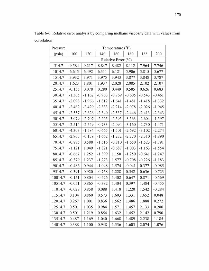
170
Table 6-6. Relative error analysis by comparing methane viscosity data with values from
correlation
Pressure Temperature (oF) (psia) 100 120 140 160 180 188 200
Relative Error (%) 514.7 9.584 9.217 8.847 8.482 8.112 7.964 7.746 1014.7 6.645 6.492 6.311 6.121 5.906 5.815 5.677 1514.7 3.932 3.971 3.975 3.943 3.877 3.848 3.787 2014.7 1.623 1.801 1.937 2.028 2.085 2.102 2.107 2514.7 -0.155 0.078 0.280 0.449 0.585 0.626 0.683 3014.7 -1.365 -1.162 -0.963 -0.769 -0.605 -0.543 -0.461 3514.7 -2.098 -1.966 -1.812 -1.641 -1.481 -1.418 -1.332 4014.7 -2.462 -2.429 -2.333 -2.214 -2.078 -2.026 -1.945 4514.7 -2.557 -2.626 -2.340 -2.537 -2.446 -2.413 -2.343 5014.7 -3.079 -2.707 -2.225 -2.595 -3.563 -2.604 -1.597 5514.7 -2.514 -2.549 -0.733 -2.094 -3.160 -2.730 -1.471 6014.7 -4.303 -1.584 -0.665 -1.501 -2.692 -3.102 -2.274 6514.7 -2.965 -0.159 -1.662 -1.272 -2.270 -2.310 -1.890 7014.7 -0.885 0.588 -1.516 -0.810 -1.650 -1.523 -1.791 7514.7 -1.121 1.049 -1.821 -0.687 -1.003 -1.163 -1.554 8014.7 -0.667 1.252 -1.399 1.150 -1.250 -0.641 -1.247 8514.7 -0.379 1.237 -1.273 1.577 -0.708 -0.226 -1.183 9014.7 -0.486 0.944 -1.048 1.574 -0.041 0.377 -0.985 9514.7 -0.391 0.920 -0.758 1.228 0.542 0.636 -0.723 10014.7 -0.151 0.804 -0.426 1.402 0.647 0.871 -0.569 10514.7 -0.051 0.865 -0.382 1.404 0.397 1.484 -0.455 11014.7 -0.028 0.858 0.088 1.418 1.220 1.542 -0.284 11514.7 0.104 0.860 0.573 1.603 1.331 1.652 0.048 12014.7 0.267 1.001 0.836 1.562 1.486 1.888 0.272 12514.7 0.501 1.035 0.984 1.571 1.457 2.133 0.280 13014.7 0.501 1.219 0.854 1.632 1.452 2.142 0.790 13514.7 0.487 1.169 1.040 1.668 1.489 2.238 1.185 14014.7 0.388 1.100 0.948 1.536 1.603 2.074 1.076

171
Table 6-6. Continued
Pressure Temperature (oF) (psia) 100 120 140 160 180 188 200
Relative Error (%) 14514.7 0.240 0.977 0.963 1.439 1.523 1.939 0.999 15014.7 0.347 0.970 0.875 1.562 1.370 1.605 1.105 15514.7 0.219 0.796 0.769 1.787 1.299 1.471 1.337 16014.7 0.038 0.875 0.805 1.068 1.380 1.356 1.456 16514.7 0.080 0.652 0.766 0.695 1.303 1.204 1.611 17014.7 -0.083 0.469 0.708 0.693 1.325 1.158 1.583 17514.7 -0.275 0.307 0.682 0.800 1.036 1.278 1.417 18014.7 -0.490 0.154 0.488 0.522 0.858 1.143 0.990 18514.7 -0.667 0.151 0.387 0.361 0.847 1.009 0.424 19014.7 -0.902 0.007 0.507 0.520 0.773 0.895 0.677 19514.7 -0.923 -0.172 0.340 0.302 0.578 0.704 0.671 20014.7 -1.082 -0.470 0.133 0.259 0.535 0.433 0.347 20514.7 -1.302 -0.623 0.190 0.115 0.498 1.043 0.325 21014.7 -2.167 -0.826 -0.126 0.003 0.353 1.106 -0.057 21514.7 -1.847 -1.108 -0.174 -0.130 0.243 0.956 -0.142 22014.7 -1.979 -1.386 -0.385 -0.262 0.023 0.862 -0.144 22514.7 -2.228 -1.977 -0.537 -0.552 -0.094 0.746 -0.060 23014.7 -2.601 -1.526 -0.605 -0.616 -0.201 0.497 -0.222 23514.7 -2.869 -2.139 -0.876 -0.569 -0.067 0.289 -0.318 24014.7 -2.941 -2.405 -1.044 -0.257 -0.458 0.060 -0.177 24514.7 -3.322 -2.579 -1.216 -0.436 -0.792 0.168 -0.284 25014.7 -3.607 - -1.315 -0.923 -1.037 - -

172
Table 6-6. Continued
Pressure Temperature (oF) (psia) 220 225 230 250 260 280 Relative Error (%)
514.7 7.376 7.282 7.194 6.833 6.645 6.285 1014.7 5.444 5.384 5.322 5.071 4.943 4.685 1514.7 3.672 3.645 3.612 3.465 3.389 3.221 2014.7 2.097 2.091 2.081 2.037 2.000 1.917 2514.7 0.749 0.765 0.775 0.797 0.799 0.786 3014.7 -0.346 -0.324 -0.304 -0.229 -0.202 -0.170 3514.7 -1.198 -1.169 -1.143 -1.044 -1.004 -0.942 4014.7 -1.820 -1.791 -1.767 -1.662 -1.616 -1.540 4514.7 -2.243 -2.455 -2.210 -2.122 -2.041 -1.972 5014.7 -2.480 -2.678 -2.580 -1.879 -2.161 -1.983 5514.7 -2.151 -2.182 -2.015 -1.664 -2.149 -2.102 6014.7 -1.827 -2.011 -1.771 -1.421 -1.990 -2.013 6514.7 -2.001 -1.819 -1.566 -1.093 -1.854 -2.098 7014.7 -0.975 -1.254 -1.360 -1.010 -1.337 -1.899 7514.7 -1.566 -0.906 -0.794 -0.861 -1.143 -1.654 8014.7 -0.908 -1.296 -0.537 -0.669 -1.330 -1.569 8514.7 -0.142 -1.105 -0.445 -0.472 -0.951 -1.437 9014.7 0.530 -0.648 -0.201 0.079 -0.832 -1.285 9514.7 0.899 -0.180 0.110 0.192 -0.504 -0.819
10014.7 1.154 0.155 0.455 0.515 -0.134 -0.671 10514.7 1.214 0.808 1.001 0.798 0.200 -0.317 11014.7 1.531 0.945 1.143 0.940 0.546 -0.213 11514.7 1.765 1.414 1.647 0.886 1.028 -0.233 12014.7 1.927 1.602 1.788 1.011 0.787 -0.147 12514.7 1.950 1.762 1.695 1.034 0.995 -0.123 13014.7 2.407 1.800 2.120 1.191 0.984 -0.032 13514.7 2.342 2.366 2.340 1.739 0.995 0.042 14014.7 2.400 1.645 2.644 1.849 1.173 -0.052

173
Table 6-6. Continued
Pressure Temperature (oF) (psia) 220 225 230 250 260 280 Relative Error (%) 14514.7 2.177 1.678 2.441 1.742 0.940 -0.059 15014.7 2.112 1.270 2.010 1.274 0.899 -0.487 15514.7 2.068 1.654 2.018 1.585 0.793 -0.161 16014.7 2.059 1.697 2.218 1.338 1.121 -0.428 16514.7 2.125 2.009 2.352 1.658 1.128 -0.309 17014.7 1.784 1.942 1.938 1.711 1.313 -0.626 17514.7 1.996 1.986 1.959 1.773 1.020 -0.438 18014.7 1.803 2.244 1.851 1.857 0.971 -0.530 18514.7 1.967 1.937 1.883 1.900 0.658 -0.478 19014.7 1.989 1.820 1.724 1.820 0.590 -0.490 19514.7 2.252 1.679 1.774 1.675 0.271 -0.654 20014.7 2.480 1.560 1.624 1.687 0.276 -0.469 20514.7 2.290 1.551 1.396 1.258 0.153 -0.662 21014.7 2.224 1.576 1.317 0.986 -0.187 -0.936 21514.7 1.878 1.335 1.266 0.596 -0.127 -0.778 22014.7 1.808 1.221 1.210 0.504 -0.324 -0.708 22514.7 1.602 1.162 1.060 0.430 -0.560 -0.757 23014.7 1.396 0.841 0.974 0.681 -0.844 -0.815 23514.7 1.124 0.611 0.840 0.818 -0.669 -0.882 24014.7 1.596 0.517 0.806 0.447 -0.047 -0.769 24514.7 1.479 0.355 1.022 0.572 -0.102 -0.785 25014.7 1.084 0.098 - - -0.141 -0.888

174
Table 6-6. Continued
Pressure Temperature (oF) (psia) 300 320 340 360 380 415 Relative Error (%)
514.7 5.929 5.578 5.224 4.881 4.537 3.944 1014.7 4.416 4.150 3.879 3.603 3.322 2.833 1514.7 3.044 2.856 2.652 2.446 2.229 1.843 2014.7 1.816 1.696 1.565 1.419 1.256 0.957 2514.7 0.744 0.683 0.608 0.511 0.405 0.181 3014.7 -0.162 -0.172 -0.208 -0.262 -0.331 -0.484 3514.7 -0.901 -0.883 -0.886 -0.903 -0.945 -1.047 4014.7 -1.484 -1.441 -1.422 -1.422 -1.438 -1.510 4514.7 -1.903 -1.834 -0.466 -1.821 -1.800 -1.929 5014.7 -1.785 -1.240 -0.914 -2.077 -1.965 -2.238 5514.7 -1.768 -1.241 -2.016 -2.248 -2.083 -2.297 6014.7 -1.580 -1.310 -2.296 -2.493 -2.520 -2.348 6514.7 -1.652 -1.478 -2.038 -2.183 -2.072 -2.665 7014.7 -1.360 -1.377 -1.607 -1.710 -1.927 -2.562 7514.7 -1.038 -1.239 -1.310 -1.732 -1.788 -2.490 8014.7 -0.861 -0.927 -1.323 -1.187 -1.680 -2.520 8514.7 -0.337 -0.677 -1.421 -2.010 -1.774 -2.206 9014.7 -0.530 -0.610 -1.903 -1.981 -1.696 -2.080 9514.7 -0.288 -0.378 -1.493 -1.718 -1.676 -1.829
10014.7 -0.178 -0.169 -1.295 -1.461 -1.308 -1.657 10514.7 0.135 -0.285 -1.281 -1.534 -1.318 -1.517 11014.7 0.451 -0.205 -1.233 -1.645 -0.887 -1.573 11514.7 0.576 -0.008 -1.011 -1.447 -0.798 -1.134 12014.7 -0.439 0.191 -1.066 -1.196 -0.794 -0.964 12514.7 -0.599 0.346 -1.120 -0.881 -0.670 -0.999 13014.7 -0.360 0.467 -1.150 -0.871 -0.717 -0.956 13514.7 -0.344 0.422 -1.022 -0.521 -0.649 -0.938 14014.7 -0.297 0.421 -1.110 -0.366 -0.582 -0.909

175
Table 6-6. Continued
Pressure Temperature (oF) (psia) 300 320 340 360 380 415 Relative Error (%) 14514.7 -0.036 0.347 -1.111 -0.242 -0.420 -0.750 15014.7 -0.172 0.239 -1.082 -0.283 -0.463 -0.583 15514.7 -0.244 -0.029 -1.388 -0.265 -0.322 -0.034 16014.7 -0.384 -0.113 -2.331 -0.349 -0.352 -0.079 16514.7 -0.705 -0.312 -2.043 -0.371 -0.370 0.132 17014.7 -0.583 -0.623 -1.973 -0.428 -0.438 -0.004 17514.7 -0.782 -0.547 -1.735 -0.439 -0.501 -0.014 18014.7 -0.952 -0.637 -2.536 -0.540 -0.507 -0.568 18514.7 -0.705 -1.192 -2.541 -0.873 -0.590 -0.245 19014.7 -0.860 -1.151 -2.491 -0.390 -0.568 -0.586 19514.7 -1.004 -0.896 -2.402 -0.533 -0.499 -0.231 20014.7 -1.073 -0.882 -2.091 -0.639 -0.410 -0.115 20514.7 -1.334 -0.877 -2.118 -0.642 -0.528 -0.302 21014.7 -1.187 -0.748 -1.998 0.146 -0.393 0.131 21514.7 -1.458 -1.038 -2.064 0.101 -0.113 0.456 22014.7 -1.629 -1.143 -1.794 0.224 -0.316 0.057 22514.7 -1.462 -1.355 -2.026 0.413 -0.444 0.511 23014.7 -1.629 -1.179 -1.665 0.589 -0.356 0.841 23514.7 -1.599 -1.502 -1.462 0.579 -0.078 0.678 24014.7 -1.932 -2.299 -1.139 0.580 -0.101 1.364 24514.7 -0.806 -2.384 -1.272 -0.544 -0.021 1.311 25014.7 - -2.516 -1.206 - -0.205 -

176
CHAPTER VII
CONCLUSIONS AND RECOMMENDATIONS
7.1 Conclusions
Upon the study we finished, following conclusions were made:
I. At high pressure, nitrogen viscosities from lab are lower than NIST values. The
difference between lab data and NIST values increases as pressure increases.
II. At high pressure, methane viscosities from lab are higher than NIST values. The
difference between lab data and NIST values increases as temperature decreases;
this difference also increases as pressure increases.
III. New gas viscosity correlations derived in this study can be used to predict gas
viscosity at HPHT confidently considering very high methane concentration in
HPHT gas reservoirs.
IV. Existing gas viscosity correlations is inappropriate for gas with moderate to high
nonhydrocarbon concentration.
V. A new nitrogen viscosity correlation based on our lab data was developed and can
be used in HPHT reservoirs containing significant amount of nitrogen.
7.2 Recommendations
Further study should focus on
I. Measuring carbon dioxide viscosity at HPHT,
II. Measuring bi-component and tri-component mixtures viscosity,
III. Measuring viscosity of natural gas sampled from HPHT reservoirs,
IV. Deriving a new correlation basing on lab data covering low to high pressure and
temperature.

177
NOMENCLATURE
Symbol Description
atm atmosphere
atms atmospheres, pressure unit
A area
A a layer in fluid flow between two plates
AA constant in friction factor equation
bar pressure unit, 1 bar = 0.987 atms
B buoyant force
B a layer in fluid flow between two plates (higher velocity than layer A)
BB constant in friction factor equation
cm centimeter
cp centipoise
CC constant in friction factor equation
CO2 carbon dioxide oC Celsius temperature
d difference
db ball diameter
D drag force
Dy drag force in y dimension, or vertical direction
Ek kinetic energy per unit volume
f friction factor
df driving force

178
Symbol Description
ff friction force
ft foot or feet
F force oF degree Fahrenheit
g gravity acceleration factor
g gram
g gas
gc gravity constant
H2S hydrogen sulfide
HPHT high pressure high temperature
in inch
kg kilogram
K constant for viscosity from capillary viscometer
K constant for viscosity correlation
Kpa thousand Pascal oK Kelvin temperature
l length, distance
m mass
m meter
mb mass of ball or sphere
Mpa million Pascal
Mw molecular weight
n number of moles
N Newton, force unit

179
Symbol Description
N2 nitrogen
NRe Reynolds number
p pressure
Δp pressure change
p1 pressure at inlet of pipe or tube
p2 pressure at outlet of pipe or tube
pi initial pressure
pc critical pressure
ppc pseudocritical pressure
psi gauge pressure
psia absolute pressure
psig gauge pressure
P poise
Pa Pascal
ppr pseudoreduced pressure
pr reduced pressure
r distance from center of circle, tube, or pipe
R radius of circle, tube, or pipe
R universal gas constant
Rgas universal gas constant
s second
sec second
SC standard condition
t time

180
Symbol Description
T temperature
Tc critical temperature
Tpc pseudocritical temperature
Tpr pseudoreduced temperature
Tr reduced temperature
u velocity
ux velocity in x direction
uy velocity in y direction
v velocity
vslip slip velocity
V volume
V1 volume above mercury in capillary tube
V2 volume below mercury in capillary tube
Vb volume of ball or sphere
Velementary elementary volume W weight x x direction or dimension X constant for viscosity correlation y y direction or dimension
2COy mole fraction of carbon dioxide in vapor
SHy2
mole fraction of hydrogen sulfide in vapor
2Ny mole fraction of nitrogen in vapor
yN2, CO2, H2S mole fraction of the non-hydrocarbon component Y constant for viscosity correlation z z-factor

181
Greek
Symbol Description
γ shear rate
gγ gas specific gravity
μ viscosity
atm1μ gas viscosity at 1 atmosphere
gμ gas viscosity
gSCμ gas viscosity at standard condition
υ kinetic viscosity
ξ constant for viscosity correlation
π a mathematical constant whose value is the ratio of any circle's
circumference to its diameter
ρ density
bρ ball or sphere density
fρ fluid density
gρ gas density
rρ reduced density
τ shear stress
ψ sphericity
Δ indicates difference
Subscripts
Symbol Description
1 inlet of the tube or pipe
1 above the mercury in capillary tube viscometer 1atm 1 atmosphere

182
Symbol Description
2 outlet of the tube or pipe
2 below the mercury in capillary tube viscometer
Avg average
CO2 carbon dioxide
g gas
H2S hydrogen sulfide
i initial
N2 nitrogen
SC low pressure condition
gSC gas at low pressure condition x x direction or dimension y y direction or dimension

183
REFERENCES
Adzumi, H. 1937. Studies on the Flow of Gaseous Mixtures through Capillaries. I The Viscosity of Binary Gaseous Mixtures. Bulletin of the Chemical Society of Japan. 12, (5): 199-226. Assael, M.J. Dalaouti, N.K. and Vesovic, V. 2001. Viscosity of Natural-Gas Mixtures: Measurements and Prediction. International Journal of Thermophysics. 22, (1): 61-71. Audonnet, F. and Padua, A.A.H. 2004. Viscosity and Density of Mixtures of Methane and n-Decane from 298 to 393 K and up to 75 MPa. Fluid Phase Equilibria. 216: 235-244. Baron J.D. Roof, J.G. and Well, F.W. 1959. Viscosity of Nitrogen, Methane, Ethane, and Propane at Elevated Temperature. Journal of Chemical and Engineering Data. 4: 283-288. Barua, A.K. Afzal, M. Flynn, G.P. and Ross, J. 1964. Viscosities of Hydrogen, Deuterium, Methane, and Carbon Monoxide from -50o to 150 oC below 200 Atmospheres. The Journal of Chemical Physics. 41: 374-378. Berwald, W.B. and Johnson, T.W. 1933. Viscosity of Natural Gases. U.S. Department of Commerce, Bureau of Mines, Technical Paper, 555. Bicher, L.B. and Katz, D.L. 1943. Viscosity of Methane-Propane System. Ind. Eng. Chem. 35: 754-761. Blasius, H. 1913. Das Aehnlichkeitsgesetz bei Reibungsvorgängen in Flüssigkeiten. Mitteilungen über Forschungsarbeiten auf dem Gebiete des Ingenieurwesens. 131: VDI-Verlag Berlin. Boon, J.P. Legros, J.C. and Thomaes, G. 1967. On the Principle of Corresponding State for the Viscosity of Simple Liquids. Physica. 33: 547-557. Bourgoyne, T.A. Chenevert, E.M. Millhein, K.K. and Young, S.F. 1986. Applied Drilling Engineering. Richardson, Texas: Textbook Series, SPE. Boyd, J. 1930. The Viscosity of Compressed Gases. Physica Review. 35: 1284-1297.

184
Cambridge Viscosity Inc. 2010. Unpublished Paper. Viscous Drag in the Oscillating Piston Viscometer, Medford, Maryland: Cambridge Viscosity, Inc. Canet, X. Baylaucq, A. and Boned, C. 2002. High-Pressure (up to 140 MPa) Dynamic Viscosity of the Methane+Decane System. International Journal of Thermophysics, 23: 1469-1486. Carmichael, L.T. Virginia, B. and Sage, B.H. 1965. Viscosities of Hydrocarbons. Methane. Journal of Chemical and Engineering Data. 10: 57-61. Carr, N.L. 1952. The Viscosity of Gas Mixtures at High Pressures. PhD thesis, Chicago, Illinois: Illinois Institute of Technology. Carr, N.L. Kobayashi, R. and Burrows, D.B. 1954. Viscosity of Hydrocarbon Gases under Pressure. Trans. AIME. 201: 264-272. Castleman, R.A. 1926. The Resistance to the Steady Motion of Small Spheres in Fluids. National Advisory Committee for Aeronautics, Technical Note No. 231, Washington D.C., February. Chan, R.K.Y. and Jackson, D.A. 1985. An Automated Falling-Cylinder High Pressure Laser-Doppler Viscometer. J. Phys. E: Sci. Instrum. 18: 510-515. Comings, E.W. and Egly, R.S. 1940. Viscosity of Gases and Vapors at High Pressures. Industrial and Engineering Chemistry. 32: 714-718. Comings, E.W. Mayland, B.J. and Egly, R.S. 1944. The Viscosity of Gases at High Pressures. Chicago, Illinois: University of Illinois Engineering Experiment Station Bulletin Series No. 354. Dabir S.V. Tushar K. Ghosh D. Prasad, H.L. Nidamartyv. K. D. and Kalipatnapu Y.R. 2007. Viscosity of Liquids-Theory, Estimation, Experiment, and Data. Columbia, Missouri: University of Missouri. Dempsey, J.R. 1965. Computer Routine Treats Gas Viscosity as a Variable. Oil and Gas Journal. 141-143, August 16. Diehl, J. Gondouin, M. Houpeurt, A. Neoschil, J. Thelliez, M. Verrien, J.P. and Zurawsky, R. 1970. Viscosity and Density of Light Paraffins, Nitrogen and Carbon Dioxide. Technip, Paris, CREPS/Geopetrole. Diller, D. E. 1980. Measurements of the Viscosity of Compressed Gases and Liquid Methane. Physica. 104A: 417-426.

185
Diller, D. E. 1983. Measurements of the Viscosity of Compressed Gases and Liquid Nitrogen. Physica. 119A: 92-100. Dipippo R. Kestin, J. and Whitelaw, J.H. 1966. A High-Temperature Oscillating-Disk Viscometer. Physica. 32: 2064-2080. Earhart, R. F. 1916. The Ratio of Specific Heats and the Coefficient of Viscosity of Natural Gas from Typical Fields. Trans. Am. Soc. Mech. Eng. 38: 983-994. Ellis, C.P. and Raw, J.R. 1959. High Temperature Gas Viscosities. II. Nitrogen, Nitric Oxide, Boron Trifluoride, Silicon Tetrafluoride, and Sulfur Hexafluoride. The Journal of Chemical Physics. 30(2): 574-576. Elsharkawy, A.M. 2004. Efficient Methods for Calculations of Compressibility, Density, and Viscosity of Natural Gases, Fluid Phase Equilibria. 218:1-13. Florida Atlantic University. 2005. Falling Ball Viscometer. http://wise.fau.edu/~blarkin/Viscometer.html. Flynn, G.P. Hanks, R.V. and Lemaire, N.A. 1963. Viscosities of Nitrogen, Helium, Neon, and Argon from -78.5o to 100 oC below 200 Atmospheres. The Journal of Chemical Physics. 38: 154-162. Giddings, J.G. James, T.F. and Riki, K. 1966. Development of a High-Pressure Capillary-Tube Viscometer and Its Application to Methane, Propane, and Their Mixtures in the Gases and Liquid Regions. The Journal of Chemical Physics. 45: 578-586. Golubev, I.F. 1959. Viscosity of Gases and Gas Mixtures, a Handbook. This book is a translation from Russian by the National Technical Information Service. Alexandria, Virginia. Gonzalez, M.H. Eakin, B.E. and Lee, A.L. 1970. Viscosity of Natural Gases. New York: Institute of Gas Technology (Chicago) Monograph on API Research Project 65. Gonzalez, M.H. Richard, F.B. and Lee, A.L. 1966. The Viscosity of Methane. Paper SPE 1483 presented at the Annual Fall Meeting, Dallas, 2-5 Oct. Grevendonk, W. Herreman, W. and De Bock, A. 1970. Measurements on the Viscosity of Liquid Nitrogen. Physica. 46: 600-604. Helleman, J.M. Kestin, J. and Ro, S.T. 1973. The Viscosity of Oxygen and Some of Its Mixtures with Other Gases, Physica. 65: 362-375.

186
Helleman, J.M. Zink, H. and Van Paemel, O. 1970. The Viscosity of Liquid Argon and Liquid Methane along Isotherms as a Function of Pressure. Physica. 46: 395-410. Herbert, T. and Stokes, G.G. 1886. The Coefficient of Viscosity of Air. Philosophical Transactions of the Royal Society of London. 177: 767-799. Hongo, M. Yokoyama, C. and Takahashi, D. 1988. Viscosity of Methane-Chlorodifluoromethane (R22) Gaseous Mixtures in the Temperature Range from 298.15 to 373.15 oK and at pressures up to 5MP. Journal of Chemical Engineering of Japan. 21: 632-639. Huang, E.T.S. Swift, G.W. and Fred, K. 1966. Viscosities of Methane and Propane at Low Temperatures and High Pressure. AIChE Journal. 12: 932-936. Iwasaki, H. 1954. Measurement of Viscosity of Gases at High Pressure. II Viscosities of Nitrogen and Mixture of Nitrogen and Hydrogen. The Chemical Research Institute of Non-Aqueous Solution. 296-307. Johnston, H.L. and McCloskey, K.E. 1940. Viscosities of Several Common Gases between 90°K and Room Temperature. The Journal of Physical Chemistry. 44(9): 1038-1058. Jossi, J.A. Stiel, L.I. and Thodos G. 1962. The Viscosity of Pure Substances in the Dense Gaseous and Liquid Phases. AIChE Journal. 8(1): 59-62. Kestin, J. and Leidenfrost, W. 1959. An Absolute Determination of the Viscosity of Eleven Gases over a Range of Pressures. Physica. 25: 1033-1062. Kestin, J. and Yata, J. 1968. Viscosity and Diffusion Coefficient of Six Binary Mixtures. The Journal of Chemical Physics. 49: 4780-4791. Klimeck, J. Kleinrahm, R. and Wagner, W. 1998. An Accurate Single-Sinker Densimeter and Measurement of the (p, ρ, T) Relation of Argon and Nitrogen in the Temperature Range from (235 to 520) K at Pressures up to 30 Mpa. J. Chem. Thermodynamics. 30: 1571-1588. Knapstad, B. Skjolsvik, P.A. and Oye, H.A. 1990. Viscosity of the n-Decane – Methane System in the Liquid Phase. Ber. Bunsenges Phys. Chem. 94: 1156-1165. Kuss, E. 1952. High pressure research II: the viscosity of compressed gases (in German). Z. Angew. Phys. 4(6): 203-207. Lambert, J.D. Cotton, K.J. Pailthorpe, M.W. Robinson, A.M. Scrivins, J. Vale, W.R.F. and Young, R.M. 1955. Transport Properties of Gaseous Hydrocarbons. Proceedings of

187
the Royal Society of London. Series A, Mathematical and Physical Sciences. 231(1185): 280-290. Latto, B., and Saunders, M.W. 1972. Viscosity of Nitrogen Gas at Low Temperatures Up to High Pressures: A New Appraisal. Physica. 46: 600-604. Lee, A.L. 1965. Viscosity of Light Hydrocarbons. New York: American Petroleum Institute, Monograph on API Research Project 65. Lee, A.L. Gonzalez, M.H. and Eakin, B.E. 1966. The Viscosity of Natural Gases. Paper SPE 1340 presented at the 1966 Annual Technical Conference and Exhibition held in Shreveport, Louisiana, 11-12 November. Lemmon, E.W. Huber, M.L. and McLinden, M.O. 2007. NIST Reference Fluid Thermodynamic and Transport Properties—REFPROP Version 8.0, User’s Guide. Physical and Chemical Properties Division, National Institute of Standards and Technology, Boulder, Colorado. Londono. F. 2001. New Correlations for Hydrocarbon Gas Viscosity and Gas Density. MS thesis, College Station, Texas: Texas A&M University, Malaguti, D. and Suitter, R. 2010. Communication between Author and Cambridge Engineers. March. Marsh, J. Zvandasara, T. Macgill, A. and Jenny, K. 2010. Material Selection for HP/HT Developments. Paper SPE 130716-MS presented at SPE International Conference on Oilfield Corrosion held in Aberdeen, United Kingdom, 24-25 May. Meyer, O.E. 1866. Viskositiit Der Kolloide. Pogg. Ann. 127: 263. Michels A. and Gibson R.O. 1931. The Measurement of the Viscosity of Gases at High Pressures: The Viscosity of Nitrogen to 1000 Atms. Proc. R. Soc. Lond. A. 134: 288-307. National Institute of Science and Technology (NIST). 2010. Web-Book of Thermodynamic Properties of Fluids. http://webbook.nist.gov,chemisty/fluid. Nowak, P. Kleinrahm, R. and Wagner, W. 1997a. Measurement and Correlation of the (p, ρ, T) Relation of Nitrogen I. The Homogeneous Gas and Liquid Regions in the Temperature Range from 55 K to 239 K at Pressures up to 12 MPa. J. Chem. Thermodynamics. 29: 1137-1156. Nowak, P. Kleinrahm, R. and Wagner, W. 1997b. Measurement and Correlation of the (p, ρ, T) Relation of Nitrogen II. Saturated Liquid and Saturated Vapor Densities and

188
Vapor Pressures along the Entire Coexistence Curve. J. Chem. Thermodynamics. 29: 1157-1174. Park, N.A. 1994. Apparatus and Method for Viscosity Measurements Using a Controlled Needle Viscometer. http://www.patentstorm.us/patents/5327778/claims.html. Paul N. Gardner Company, Inc. 2010. Vibrational Viscometer Based on Tuning Fork Technology. http://www.gardco.com/pages/viscosity/viscometers/sv_10_100.html. Rankine, A.O. 1910. On a Method of Determining the Viscosity of Gases, Especially Those Available only in Small Quantities. Proc. Roy. Soc. 83A: 265-276. Rankine, A.O. 1923. A Simple Viscometer for Gases. J. Sci. Instr. 1: 105-111 Rudenko, N.S. and Schubnikow, L.W. 1934. The Viscosity of Liquid Nitrogen, Carbon Monoxide, Argon and Oxygen as a Function of Temperature. Physikalische Zeitschrift Sowjetunion. 6: 470-477. Ross, J. and Brown, G. 1957. Viscosity of Gases at High Pressures. Ind. Eng. Chem. 49: 2026-2033. Sage, B.H. and Lacey, W.N. 1938. Effect of Pressure upon Viscosity of Methane and Two Natural Gases. Trans. Am. Inst. Mining Met. Engrs. 127: 118-134. Schley, P. Jaeschke, M. Kuchenmeister, C. and Vogel E. 2004. Viscosity Measurements and Predictions for Natural Gas. International Journal of Thermophysics. 25: 1623-1652. Seibt, D. Vogel, E. Bich, E. Buttig, D. and Hassel, E. 2006. Viscosity Measurements on Nitrogen. J. Chem. Eng. Data. 51: 526-533. Setzmann, U. and Wagner, W. 1991. A New Equation of State and Tables of Thermodynamic Properties for Methane Covering the Range from the Melting Line to 625 K at Pressures up to 1000 MPa. J. Phys. Chem. Ref. Data. 20(6): 1061-1155. Smith, A.S. and Brown, G.G. 1943. Correlating Fluid Viscosity. Ind. Eng. Chem. 35: 705-711. Steffe, J.F. 1992. An Oscillating Sphere System for Creating Controlled Amplitude in Liquid, Rheological Methods in Food Process Engineering. Michigan, Illinois: Freeman Press. Stephan, K. and Lucas, K. 1979. Viscosity of Dense Fluids. West Lafayette, Indiana: The Purdue Research Foundation.

189
Stewart, J.R. 1952. The Viscosity of Natural Gas Components at High Pressure. Master thesis, Chicago, Illinois: Illinois Institute of Technology. Stokes, G.G. 1868. On the Communication of Vibration from a Vibrating Body to a Surrounding Gas. Philosophical Transactions of the Royal Society of London. 158: 447-463. Straty, G.C. and Diller, D.E. 1980. PVT of Saturated and Compressed Fluid Nitrogen. J. Chem. Thermodynamics. 12: 927-936. Sutton, R.P. 2005. Fundamental PVT Calculations for Associated and Gas/Condensate Natural-Gas Systems. Paper SPE 97099 presented at the SPE Annual Technical Conference and Exhibition, Dallas, Texas, 9–12 October. Swift, G.W. Christy, J.A. and Kurata, F. 1959. Liquid Viscosities of Methane and Propane. AIChE Journal. 5: 98-102. Swift, G.W. Lorenz J. and Kurata, F. 1960. Liquid Viscosities above the Normal Boiling Point for Methane, Ethane, Propane, and n-Butane. AIChE Journal. 6: 415-419. Tomida, D. Kumagai, A. and Yokoyama, C. 2005. Viscosity Measurements and Correlation of the Squalane + CO2 Mixture. International Journal of Thermophysics, 28(1): 133-145. Trautz, M. and Zink, R. 1930. The Viscosity, Thermal Conductivity and Diffusion in Gas Mixtures. XII. Gas Viscosity at High Temperatures (in German). Ann. Phys. (Leipzig). 7: 427-452. Van Der Gulik, P. S. Mostert, R. and Van Den Berg, H. R. 1988. The Viscosity of Methane at 25 oC up to 10 kbar. Physica. 151A: 153-166. Van Itterbeek, A. Hellemans, J. Zink, H. and Van Cauteren, M. 1966. Viscosity of Liquefied Gases at Pressures between 1 and 100 Atmosphere. Physica. 32: 2171-2172. Van Itterbeek A. Van Paemel, O. and Van Lierde, J. 1947. Measurements on the Viscosity of Gas Mixtures. Physica XlII. 1-3: 88-96. Viswanathan, A. 2007. Viscosities of Natural Gases at High Pressures and High Temperatures. Master thesis, College Station, Texas: Texas A&M University. Viswanathan, A. and McCain Jr., W.D. 2005. Crisman Institute for Petroleum Research Monthly Report, April 2005. Department of Petroleum Engineering, College Station: Texas A&M University.

190
Viswanathan, A. McCain Jr. W.D., and Teodoriu, C. 2006. Crisman Institute for Petroleum Research Monthly Report, March to December 2006. Department of Petroleum Engineering, College Station: Texas A&M University. Vogel, E. Wilhelm, J. Cornelia, K. and Manfred, J. 1999. High-Precision Viscosity Measurements on Methane. Presented at the 15th European Conference on Thermophysical Properties, Wurzburg, Germany, 5-9 September. Wikipedia. 2009. Definition of Fanning Friction Factor. http://en.wikipedia.org/wiki/Fanning_friction factor. Wikipedia. 2010. Viscosity. http://en.wikipedia.org/wiki/Viscosity. Wilson, J. 1965. A Method of Predicting the Viscosities of Natural Gases for a Wide Range of Pressures and Temperatures. PhD dissertation, College Station, Texas: Texas A&M University. Yen, K. 1919. LVIII. An Absolute Determination of the Coefficients of Viscosity of Hydrogen, Nitrogen, and Oxygen. Philosophical Magazine Series 6. Vol. 28, Issue 227, Page 582-596. Zhang, Zh. Fu, J. Lin, Y. Fan, H. Xia, B. and Zhang, J. 2010. The Mechanism of Pressure Control Problem in High H2S/CO2 Gas Wells. Paper SPE 130143-MS presented at CPS/SPE International Oil & Gas Conference and Exhibition in China held in Beijing, China, 8-10 June.
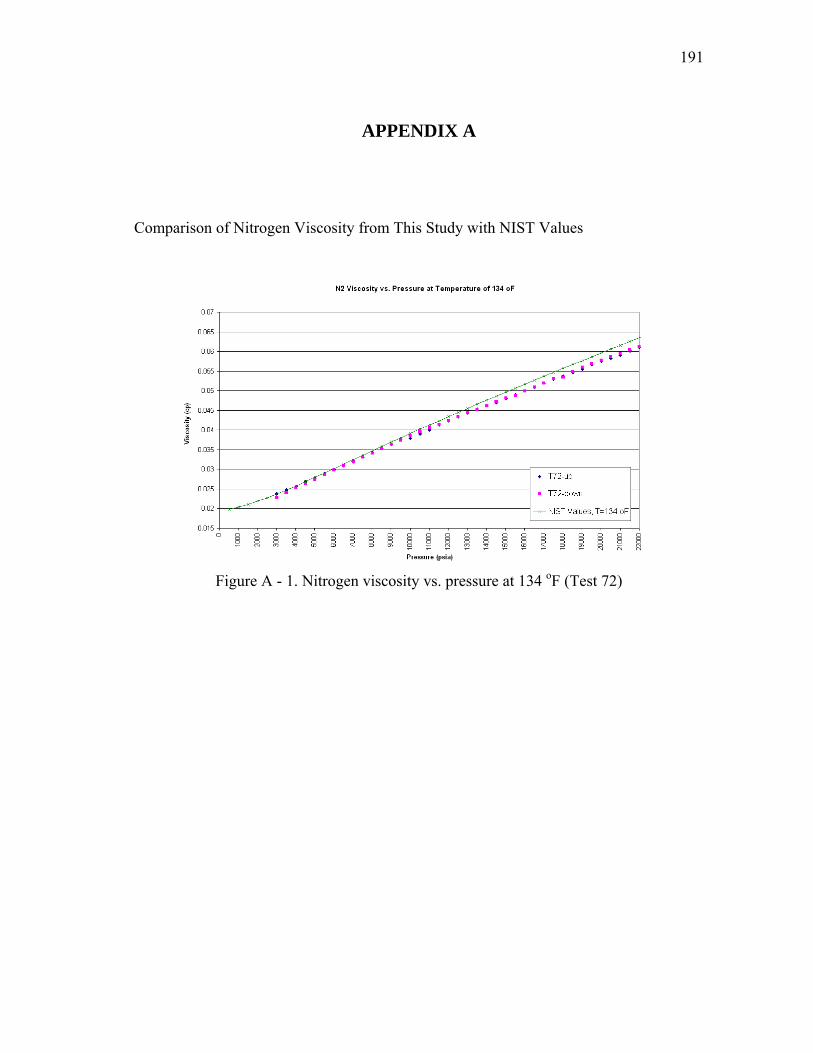
191
APPENDIX A
Comparison of Nitrogen Viscosity from This Study with NIST Values
Figure A - 1. Nitrogen viscosity vs. pressure at 134 oF (Test 72)

192
Figure A - 2. Nitrogen viscosity vs. pressure at 134 oF (Test 73)
Figure A - 3. Nitrogen viscosity vs. pressure at 134 oF (Test74)

193
Figure A - 4. Nitrogen viscosity vs. pressure at 152 oF (Test 75)
Figure A - 5. Nitrogen viscosity vs. pressure at 152 oF (Test 76)

194
Figure A - 6. Nitrogen viscosity vs. pressure at 152 oF (Test 77)
Figure A - 7. Nitrogen viscosity vs. pressure at 170 oF (Test 78)

195
Figure A - 8. Nitrogen viscosity vs. pressure at 170 oF (Test 79)
Figure A - 9. Nitrogen viscosity vs. pressure at 170 oF (Test 80)

196
Figure A - 10. Nitrogen viscosity vs. pressure at 170 oF (Test 81)
Figure A - 11. Nitrogen viscosity vs. pressure at 200 oF (Test 82)

197
Figure A - 12. Nitrogen viscosity vs. pressure at 200 oF (Test 83)
Figure A - 13. Nitrogen viscosity vs. pressure at 250 oF (Test 63)

198
Figure A - 14. Nitrogen viscosity vs. pressure at 250 oF (Test 64)
Figure A - 15. Nitrogen viscosity vs. pressure at 250 oF (Test 65)

199
Figure A - 16. Nitrogen viscosity vs. pressure at 250 oF (Test 66)
Figure A - 17. Nitrogen viscosity vs. pressure at 260 oF (Test 67)

200
Figure A - 18. Nitrogen viscosity vs. pressure at 260 oF (Test 84)
Figure A - 19. Nitrogen viscosity vs. pressure at 260 oF (Test 85)

201
Figure A - 20. Nitrogen viscosity vs. pressure at 280 oF (Test 86)
Figure A - 21. Nitrogen viscosity vs. pressure at 280 oF (Test 87)

202
Figure A - 22. Nitrogen viscosity vs. pressure at 300 oF (Test 88)
Figure A - 23. Nitrogen viscosity vs. pressure at 300 oF (Test 89)

203
Figure A - 24. Nitrogen viscosity vs. pressure at 330 oF (Test 90)
Figure A - 25. Nitrogen viscosity vs. pressure at 330 oF (Test 91)
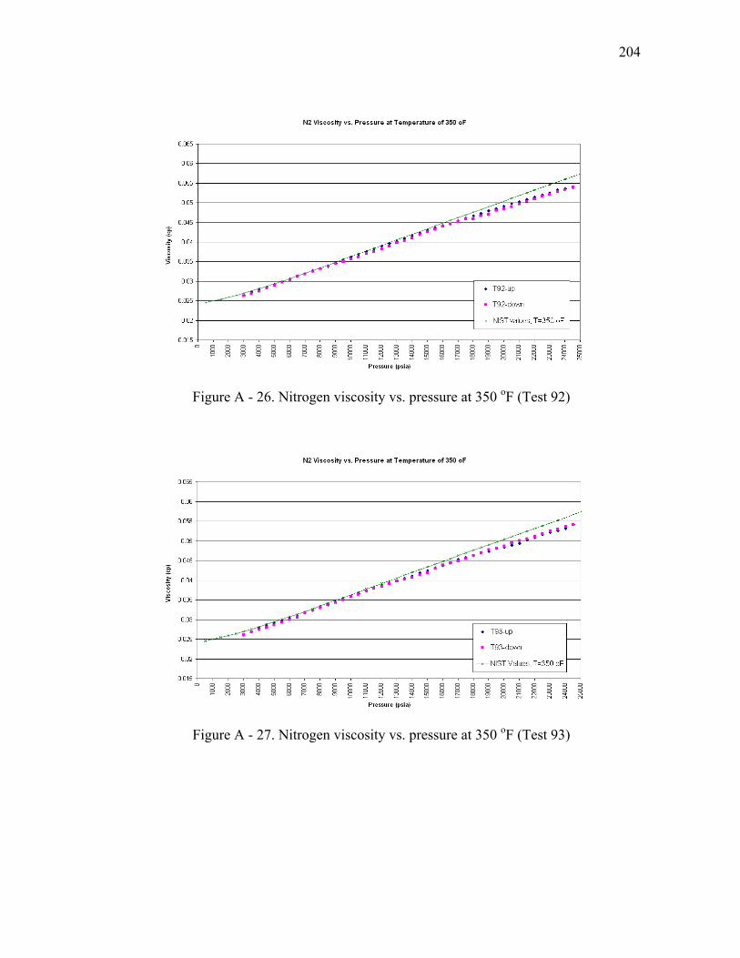
204
Figure A - 26. Nitrogen viscosity vs. pressure at 350 oF (Test 92)
Figure A - 27. Nitrogen viscosity vs. pressure at 350 oF (Test 93)

205
APPENDIX B
Comparison of Methane Viscosity from This Study with NIST Value
Figure B - 1. Methane viscosity vs. pressure at 120 oF (Test 48)

206
Figure B - 2. Methane viscosity vs. pressure at 120 oF (Test 49)
Figure B - 3. Methane viscosity vs. pressure at 140 oF (Test 46)

207
Figure B - 4. Methane viscosity vs. pressure at 140 oF (Test 47)
Figure B - 5. Methane viscosity vs. pressure at 160 oF (Test 44)

208
Figure B - 6. Methane viscosity vs. pressure at 160 oF (Test 45)
Figure B - 7. Methane viscosity vs. pressure at 180 oF (Test 42)

209
Figure B - 8. Methane viscosity vs. pressure at 180 oF (Test 43)
Figure B - 9. Methane viscosity vs. pressure at 188 oF (Test 13)

210
Figure B - 10. Methane viscosity vs. pressure at 188 oF (Test 14)
Figure B - 11. Methane viscosity vs. pressure at 188 oF (Test 15)

211
Figure B - 12. Methane viscosity vs. pressure at 200 oF (Test 16)
Figure B - 13. Methane viscosity vs. pressure at 200 oF (Test 17)

212
Figure B - 14. Methane viscosity vs. pressure at 200 oF (Test 18)
Figure B - 15. Methane viscosity vs. pressure at 220 oF (Test 19)

213
Figure B - 16. Methane viscosity vs. pressure at 220 oF (Test 20)
Figure B - 17. Methane viscosity vs. pressure at 220 oF (Test 21)

214
Figure B - 18. Methane viscosity vs. pressure at 225 oF (Test 22)
Figure B - 19. Methane viscosity vs. pressure at 230 oF (Test 23)
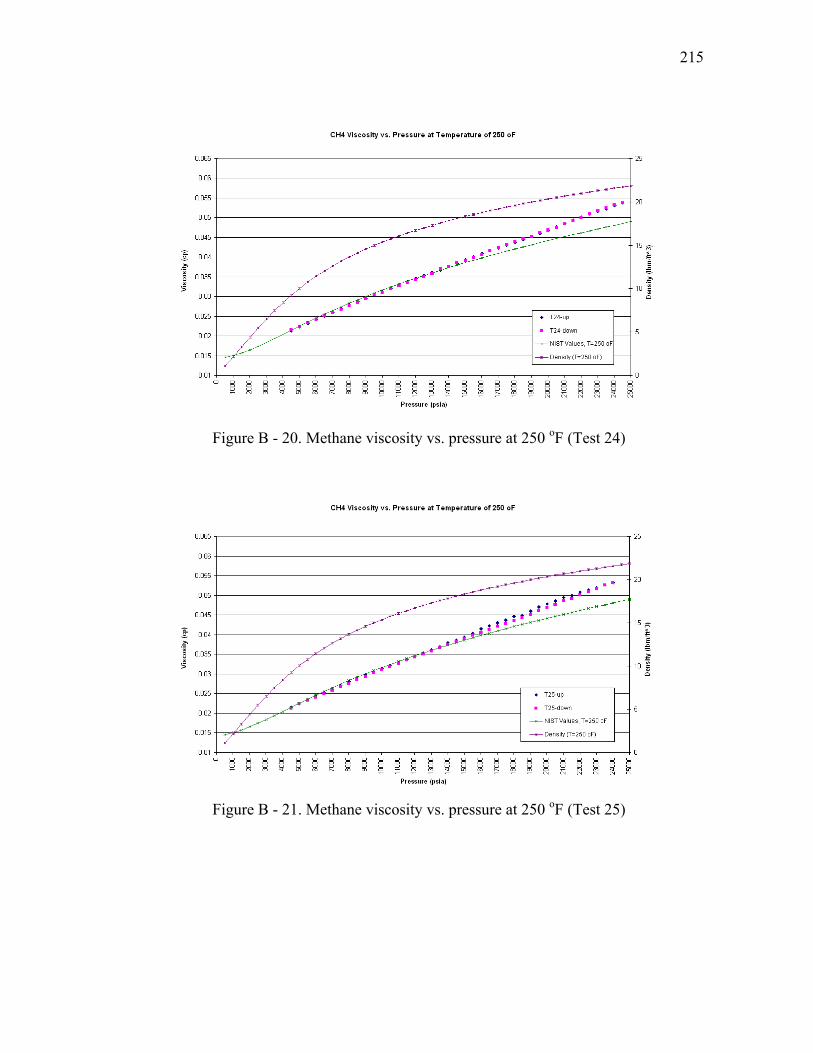
215
Figure B - 20. Methane viscosity vs. pressure at 250 oF (Test 24)
Figure B - 21. Methane viscosity vs. pressure at 250 oF (Test 25)

216
Figure B - 22. Methane viscosity vs. pressure at 260 oF (Test 26)
Figure B - 23. Methane viscosity vs. pressure at 260 oF (Test 27)

217
Figure B - 24. Methane viscosity vs. pressure at 280 oF (Test 28)
Figure B - 25. Methane viscosity vs. pressure at 280 oF (Test 29)

218
Figure B - 26. Methane viscosity vs. pressure at 300 oF (Test 30)
Figure B - 27. Methane viscosity vs. pressure at 300 oF (Test 31)

219
Figure B - 28. Methane viscosity vs. pressure at 320 oF (Test 32)
Figure B - 29. Methane viscosity vs. pressure at 320 oF (Test 33)

220
Figure B - 30. Methane viscosity vs. pressure at 340 oF (Test 34)
Figure B - 31. Methane viscosity vs. pressure at 340 oF (Test 35)

221
Figure B - 32. Methane viscosity vs. pressure at 360 oF (Test 36)
Figure B - 33. Methane viscosity vs. pressure at 360 oF (Test 37)

222
Figure B - 34. Methane viscosity vs. pressure at 380 oF (Test 38)
Figure B - 35. Methane viscosity vs. pressure at 380 oF (Test 39)
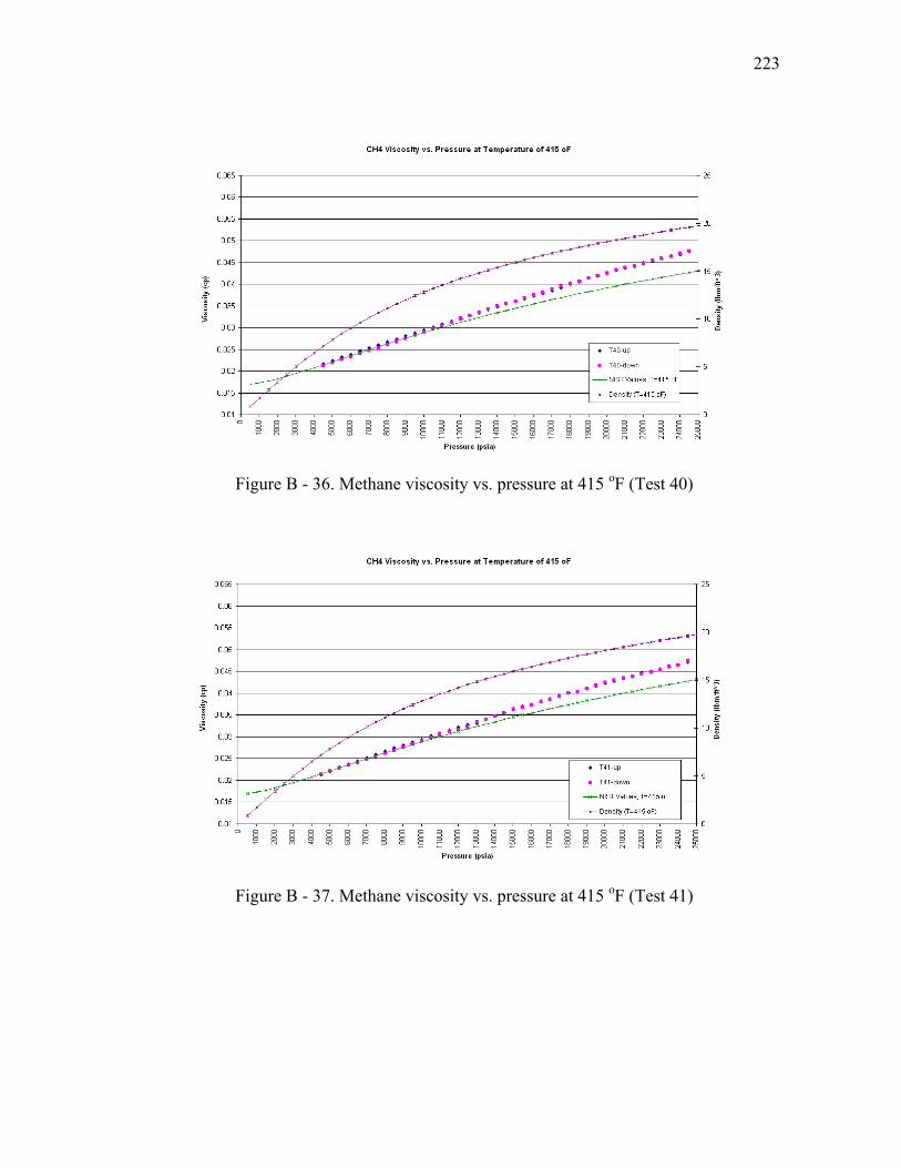
223
Figure B - 36. Methane viscosity vs. pressure at 415 oF (Test 40)
Figure B - 37. Methane viscosity vs. pressure at 415 oF (Test 41)

224
VITA
Name: Kegang Ling Contact Information: Department of Petroleum Engineering Texas A&M University 3116 TAMU Richardson Building College Station, TX 77843-3116 Email Address: [email protected] Education: M.S., Petroleum Engineering, University of Louisiana at Lafayette, 2006 B.S., Geology, China Petroleum University, 1995 Professional Affiliation: Society of Petroleum Engineers, Member