Universal Journal of Physics and Application 10(4): 128-140, 2016 DOI: 10.13189/ujpa.2016.100404 http://www.hrpub.org

General Classical Electrodynamics

Koen J. van Vlaenderen

Ethergy B.V, Research, Hobbemalaan 10, 1816GD Alkmaar, North Holland, The Netherlands Institute for Basic Research, P.O. Box 1577, Palm Harbor, FL 34684 U.S.A.

Copyright c©2016 by authors, all rights reserved. Authors agree that this article remains permanently

open access under the terms of the Creative Commons Attribution License 4.0 International License

Abstract Maxwell’s Classical Electrodynamics (MCED)suffers several inconsistencies: (1) the Lorentz force law ofMCED violates Newton’s Third Law of Motion (N3LM) incase of stationary and divergent or convergent current distri-butions; (2) the general Jefimenko electric field solution ofMCED shows two longitudinal far fields that are not waves;(3) the ratio of the electrodynamic energy-momentum of acharged sphere in uniform motion has an incorrect factorof 4

3 . A consistent General Classical Electrodynamics(GCED) is presented that is based on Whittaker’s reciprocalforce law that satisfies N3LM. The Whittaker force isexpressed as a scalar magnetic field force, added to theLorentz force. GCED is consistent only if it is assumedthat the electric potential velocity in vacuum, ’a’, is muchgreater than ’c’ (a � c); GCED reduces to MCED, in casewe assume a = c. Longitudinal electromagnetic wavesand superluminal longitudinal electric potential waves arepredicted. This theory has been verified by seeminglyunrelated experiments, such as the detection of superluminalCoulomb fields and longitudinal Ampere forces, and has awide range of electrical engineering applications.

Keywords Classical Electrodynamics, LongitudinalAmpere Force, Scalar Fields, Longitudinal Electric Waves,Superluminal Velocity, Energy Conversion

1 Introduction

An alternative to Maxwell’s [1, 2] Classical Electrodynam-ics (MCED) theory is presented, called General ClassicalElectrodynamics (GCED), that is free of inconsistencies. Forthe development of this theory we make use of the fundamen-tal theorem of vector algebra. The proof of this fundamentaltheorem is based on the three dimensional delta function δ(x)and the sifting property of this function, see (1.1 – 1.2):

δ(x) =−1

4π∆

(1

|x|

)(1.1)

F(x) =

∫V ′

F(x′) δ(x− x′) d3x′ (1.2)

The fundamental theorem of vector algebra is as follows: avector function F(x) can be decomposed into two uniquevector functions Fl(x) and Ft(x), such that

F(x) = Fl(x) + Ft(x) (1.3)

Fl(x) = − 1

4π∇∫V ′

∇′ · F(x′)

|x− x′| d3x′ (1.4)

Ft(x) =1

4π∇×

∫V ′

∇′ × F(x′)

|x− x′| d3x′ (1.5)

The lowercase subindexes ’l’ and ’t’ will have the meaningof longitudinal and transverse in this paper. The longitudinalvector function Fl is curl free (∇×Fl = 0), and the trans-verse vector function Ft is divergence free (∇·Ft = 0). Weassume that F is well behaved (F is zero if |x| is infinite). Letus further introduce the following notations and definitions.

ρ Net electric charge density, in C/m3

J = Jl + Jt Net electric current density, in A/m2

Φ Net electric charge (scalar) potential, in V

A = Al + At Net electric current (vector) potential,

in V·s/m

EΦ = −∇Φ Electric field, in V/m

EL = −∂tAl Field induced divergent electric field

ET = −∂tAt Field induced rotational electric field

BΦ = −∂tΦ Field induced scalar field, in V/s

BL = −∇·Al Scalar magnetic field, in T = V·s/m2

BT = ∇×At Vector magnetic field, in T = V·s/m2

φ0 � ε20µ0 Polarizability of vacuum, in F·s2/m3

µ0 Permeability of vacuum: 4π10−7 H/m

ε0 Permittivity of vacuum: 8.854−12 F/m

Universal Journal of Physics and Application 10(4): 128-140, 2016 129

(x, t) = (x, y, z, t) Place and time coordinates

∂t =∂

∂tPartial time differential

∇=

(∂

∂x,∂

∂y,∂

∂z

)Del operator

∆ = ∇ · ∇ Laplace operator

∆Φ = ∇·∇Φ, ∆A = ∇∇·A−∇×∇×A

The permittivity, permeability and polarizability of vacuumare constants. The charge- and current density distributions,the potentials and the fields, are functions of place and notalways functions of time. Time independent functions arecalled stationary or static functions. Basically there are threetypes of charge-current density distributions:

A. Current free charge J = 0B. Stationary currents ∂tJ = 0

1. closed circuit ∂tJ = 0 ∧ ∇·J = 02. open circuit ∂tJ = 0 ∧ ∇·J 6= 0

C. Time dependent currents ∂tJ 6= 0

The charge conservation law (also called ’charge continuity’)is true for all types of charge-current density distributions:

∂ρ

∂t+∇·J = 0 (1.6)

The physics of current free charge density distributions iscalled Electrostatics (ES): ∂tρ = −∇·0 = 0. The physicsof stationary current density distributions (∂tJ = 0) is calledGeneral Magnetostatics (GMS). A special case of GMS aredivergence free current distributions (∇·J = 0), and thisis widely called Magnetostatics (MS) in the scientific educa-tional literature. In case of Magnetostatics, the charge densitydistribution has to be static as well: ∂tρ = −∇·J = 0, suchthat the electric field and the magnetic field are both static.

The Maxwell-Lorentz force law satisfies Newton’s thirdlaw of motion (N3LM) in case of Electrostatics and Magne-tostatics, however, this force law violates N3LM in case ofGeneral Magnetostatics. A violation of N3LM means thatmomentum is not conserved by GMS systems, for whichthere is no experimental evidence! This remarkable inconsis-tency in classical physics is rarely mentioned in the scientificeducational literature.

This is not the only problematic aspects of MCED. Jefi-menko’s electric field expression that is derived from MCEDtheory, shows two longitudinal electric field terms that do notinteract by induction with other fields, therefore these electricfields cannot be field waves and nevertheless these electricfields fall off in magnitude by distance, as far fields, which isinconsistent. A third inconsistency is the problematic 4

3 fac-tor in the ratio of the electric energy and the electromagneticmomentum of a charged sphere. In the next sections we de-scribe these related inconsistencies of MCED theory in moredetail, and how to resolve them.

2 General Magnetostatics

Let J(x) be a stationary current distribution. The vectorpotential A(x) at place vector x is given by:

A(x) =µ0

4π

∫V ′

J(x′)

rd3x′ (2.1)

r = x− x′

r = |x− x′|

Since ∂tA = 0 for stationary currents, the electric fieldequals E = EΦ = −∇Φ, such that the Gauss law for GeneralMagnetostatics is given by

∇·EΦ(x, t) =1

ε0ρ(x, t) (2.2)

The magnetostatic vector field BT (x) is defined by Biot-Savart’s law as follows:

BT (x) = ∇×At(x) = ∇×A(x)

= − µ0

4π

∫V ′

J(x′)×∇(

1

r

)d3x′

=µ0

4π

∫V ′

1

r3

[J(x′)× r

]d3x′ (2.3)

The magnetic field is indeed static, since the current densityis stationary. From the continuity of charge (1.6), and (2.2),it follows that Jl = −ε0∂t(EΦ), hence the Ampere law forGeneral Magnetostatics is as follows:

∇×BT − ε0µ0∂EΦ

∂t= µ0J (2.4)

2.1 The Lorentz forceThe magnetic force density, fT (x), that acts transversely

on current density J(x) at place x, is given by:

fT (x) = J(x)×BT (x)

=µ0

4π

∫V ′

1

r3J(x)×

[J(x′)× r

]d3x′

=µ0

4π

∫V ′

1

r3

[[J(x) · r

]J(x′) −

[J(x′) · J(x)

]r]

d3x′

=µ0

4π

∫V ′

fT (x,x′) d3x′ (2.5)

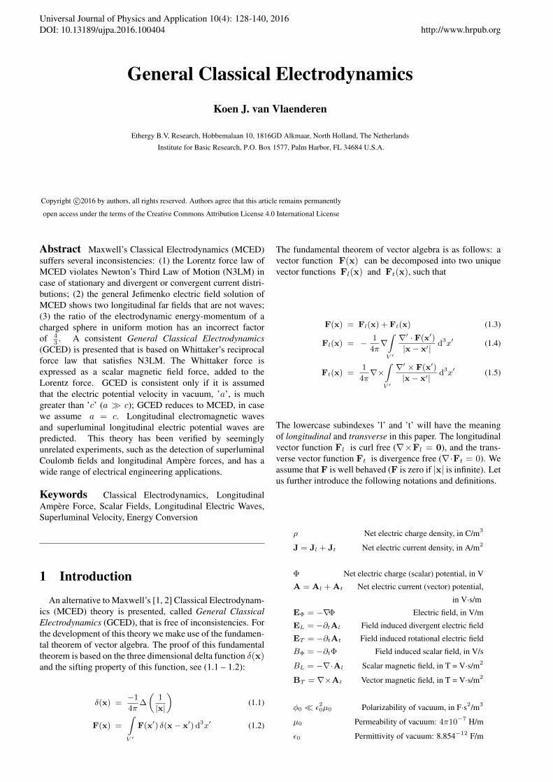
This is the Lorentz force density law for Magnetostatics; itis assumed that the electric force densities are negligible.Notice that the integrand is non-reciprocal: fT (x,x′) 6=−fT (x′,x), and that r changes into −r by swapping x andx′. This means that the Lorentz force law agrees with N3LM,but only if one calculates the total force on closed on-itselfcurrent circuits (magnetostatics is usually defined for diver-gence free currents only), which is proven as follows.Consider two non-intersecting and closed current circuits Cand C ′, that carry the stationary electric currents I and I ′,see figure 1. The currents I and I ′ are equal to the surfaceintegral of the current density over a circuit line cross sec-tion of respectively circuits C and C ′. The total force actingon circuit C is a double volume integral of the Lorentz forcedensity. We assume that the currents in C and C ′ are con-stant for each circuit line cross section, therefore we replacethe double volume integral by a double line integral over thecircuits C and C ′, in order to determine the force, FC , actingon C:

130 General Classical Electrodynamics

I

I ′

dl

dl′

r

x x′

O

Figure 1. Closed stationary current circuits

FC = −µ0II′

4π

∮C

∮C′

dl× (dl′ ×∇[

1

r

])

= −µ0II′

4π

∮C′

∮C

[(dl · ∇

[1

r

])dl′ − (dl · dl′)∇

[1

r

] ]=

µ0II′

4π

∮C

∮C′

(dl · dl′)∇[

1

r

](2.6)

This is Grassmann’s [3] force law for closed current circuits.Since the curl of a gradient is zero, the first integral disap-pears, see (2.6) after the first derivation. The final integralafter derivation step 2 has a reciprocal integrand, such thatthe force acting on circuitC ′ is the exact opposite of the forceacting on circuitC (FC = −FC′ ), in agreement with N3LM.Fubini’s theorem is applicable in derivation step 1 (switchingthe integration order in the first integral), since it is assumedthe circuits C and C ′ do not intersect.

The standard literature on Classical Electrodynamics usu-ally defines Magnetostatics as the physics of stationary anddivergence free (closed circuits) electric currents. For ex-ample, the Feynman lectures [4, Vol II, §13.4] describe thatMagnetostatics is based on equation∇×BT = µJ, such thatMagnetostatic current is divergence free, such that the elec-tric field is also static, and such that charge density is con-stant in time: ∇·J = 0 = ∂tρ. R. Feynman further suggeststhat a Magnetostatic circuit may contain batteries or genera-tors that keep the charges flowing, however, an electric bat-tery delivers an electrical current only if the battery’s chargedensity changes in time. A generator of stationary currentis for example Faraday’s homopolar disk generator, whichcan be included in a stationary closed current loop. One hasto measure the force FC on the entire closed circuit that in-cludes the generator as well, while the generator is externallydriven with constant speed. Such a magnetostatic force ex-periment has yet to be done. J. D. Jackson’s [5] third editionof Classical Electrodynamics postulates without proof that∇·J = 0 = ∂tρ (charge density is time-independent any-where in space, see after equation 5.3) before Jackson treatsthe laws of magnetostatics. D. J. Griffiths’ [6] treatment ofmagnetostatics is likewise: ”stationary electric currents aresuch that the density of charge is constant anywhere”, whichmeans that stationary currents that are divergence free. A.Altland [7] defined ’statics’ as ’static electric fields and staticmagnetic fields’, and again this implies that∇·J = 0 = ∂tρ.

Etc ...It is not at all straightforward to find practical examples of

a measured force exerted on a stationary and perfectly closed-on-itself current circuit. The Meisner effect might be such anexample: a free falling permanent magnet approaches a su-perconductor, which induces a closed-circuit current in thesuperconductor. The magnet falls until the induced currentsand magnetic field of the superconductor perfectly opposesthe field of the magnet, which causes the magnet to levitate,and from that moment on the superconductor current is sta-tionary and divergence free. However, we cannot measure the”electric current” of the floating permanent magnet, in orderto derive a magnetostatics force law. An electrically chargedrotating object may represent a closed-circuit stationary cur-rent, however, it seems impractical to measure forces on suchobjects while keeping the rotation speed constant during themeasurements. Ampere force experiments with two coils thatconduct stationary currents have been performed frequentlyin history. A coil with several windings gives the impressionof a perfectly closed current loop, however, this is only trueapproximately.

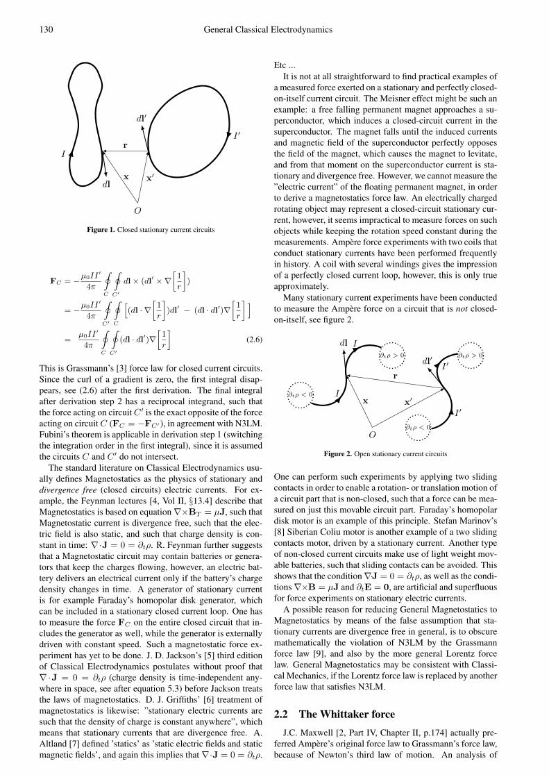
Many stationary current experiments have been conductedto measure the Ampere force on a circuit that is not closed-on-itself, see figure 2.

∂tρ < 0

∂tρ > 0 ∂tρ > 0

∂tρ < 0

O

I

I

I ′

I ′

dl

dl′

x x′

r

Figure 2. Open stationary current circuits

One can perform such experiments by applying two slidingcontacts in order to enable a rotation- or translation motion ofa circuit part that is non-closed, such that a force can be mea-sured on just this movable circuit part. Faraday’s homopolardisk motor is an example of this principle. Stefan Marinov’s[8] Siberian Coliu motor is another example of a two slidingcontacts motor, driven by a stationary current. Another typeof non-closed current circuits make use of light weight mov-able batteries, such that sliding contacts can be avoided. Thisshows that the condition∇·J = 0 = ∂tρ, as well as the condi-tions∇×B = µJ and ∂tE = 0, are artificial and superfluousfor force experiments on stationary electric currents.

A possible reason for reducing General Magnetostatics toMagnetostatics by means of the false assumption that sta-tionary currents are divergence free in general, is to obscuremathematically the violation of N3LM by the Grassmannforce law [9], and also by the more general Lorentz forcelaw. General Magnetostatics may be consistent with Classi-cal Mechanics, if the Lorentz force law is replaced by anotherforce law that satisfies N3LM.

2.2 The Whittaker forceJ.C. Maxwell [2, Part IV, Chapter II, p.174] actually pre-

ferred Ampere’s original force law to Grassmann’s force law,because of Newton’s third law of motion. An analysis of

Universal Journal of Physics and Application 10(4): 128-140, 2016 131

Ampere’s force law by E. T. Whittaker [10, p.91], resulted inthe following Whittaker force law,

FC =µ0II

′

4π

∫C

∫C′

1

r3

[(dl′ ·r)dl+(dl ·r)dl′−(dl ·dl′)r)

](2.7)

that is equal to Grassmann’s force law (2.6), except for theadditional term (dl′ · r)dl. Both force laws predict the sameforce acting on closed on-itself circuits, since the line integralof the additional term over a closed circuit disappears as well.However, Whittaker’s force law is reciprocal (FC = −FC′ ),also for non-closed circuits, and satisfies N3LM for GeneralMagnetostatics.

By means of the following functions, defined as follows,

BL(x) = −∇·Al(x) = −∇·A(x)

= −µ0

4π

∫V ′

J(x′) · ∇(

1

r

)d3x′

=µ0

4π

∫V ′

1

r3

[J(x′) · r

]d3x′ (2.8)

fL(x) = J(x)BL(x) (2.9)

we generalize Whittaker’s force law as a double volume inte-gral of field force densities, see [11, equation 13], and [12]:

∫V

[fL(x) + fT (x)

]d3x =

∫V

[J(x)BL(x) + J(x)×BT (x)

]d3x =

µ0

4π

∫V

∫V ′

1

r3

[[J(x′) · r

]J(x) +

[J(x) · r

]J(x′) −

[J(x′) · J(x)

]r

]d3x′ d3x (2.10)

This double volume integral of force densities satisfiesN3LM for stationary current densities in general, since theintegrand is reciprocal. The additional force density, fL, iscalled the longitudinal Ampere force density, which balancesthe transverse Ampere force density, fT , such that the to-tal Ampere force density f(x) = fL(x) + fT (x) satisfiesf(x) = −f(x′), see figure 3.

O

J(x) J(x′)

xx′

f(x)

fL(x)

fT (x)

fL(x′)

f(x′)

fT (x′)

Figure 3. Total Ampere force density

It is obvious that the scalar function BL is a physical fieldthat mediates an observable Ampere force, just like the vec-tor magnetic field BT , and therefore it is called the scalarmagnetic field [13].

2.3 The Lorenz conditionBy means of (1.1), (1.2) and (2.3), (2.8), we derive the

following equations:

∇BL(x) +∇×BT (x) = −∆A(x) = µ0J(x) (2.11)

∇BL(x) = −∇∇·Al(x) = µ0Jl(x) (2.12)

∇×BT (x) = ∇×∇×At(x) = µ0Jt(x) (2.13)

The following GMS condition follows from (2.4), (2.11) and(3.1), and is known as the Lorenz condition [14]:

∇( BL + ε0µ0BΦ ) = 0 (2.14)

This GMS condition is not a free to choose ”gauge” condi-tion. If the scalar function BL has the meaning of a physicalfield, then Lorenz’s condition shows that the scalar functionBΦ also has the meaning of a physical field. So far we haveshown a consistent GMS theory in agreement with classicalmechanics.

3 General CEDWe continue to develop the theory of General CED that

describes the physics of time dependent currents, taking intoaccount the physical scalar fields BL, BΦ and (2.2), (2.12)and (2.13).

3.1 General field inductionThe field equations that describe the induction of sec-

ondary fields by primary time dependent fields, follow di-rectly from the field definitions and the fact that the operators∇,∇· and ∇× commute with ∂t:

∇BΦ −∂EΦ

∂t= −∇∂Φ

∂t+∂(∇Φ)

∂t= 0 (3.1)

∇·EL −∂BL

∂t= −∇· ∂Al

∂t+∂(∇·Al)

∂t= 0 (3.2)

∇×ET +∂BT

∂t= −∇× ∂At

∂t+∂(∇×At)

∂t= 0 (3.3)

This is the generalization of Faraday’s [15] law of induction,see (3.3). A curl-free electric field EL is induced by a timevarying scalar magnetic field BL, see (3.2), which is simi-lar to the Faraday induction of a divergence-free electric fieldET . Equation (3.2) will be called Nikolaev’s [13] law of elec-tromagnetic induction, after G.V. Nikolaev.

Electric fields are sourced by static charges and induced bytime varying vector- and scalar magnetic fields. Accordingto the superposition principle, a superimposed electric fieldis defined as E = EΦ + EL + ET = −∇Φ − ∂tA. Noticethat El = EΦ + EL and that Et = ET .

3.2 The essence of Maxwell’s CEDMaxwell’s famous treatise on electricity and magnetism

does not include the definitions of the fields BL and BΦ,and does not include Nikolaev’s induction law. However,Maxwell defined the superimposed electric field as E =EΦ +EL +ET , without explaining the induction of the sec-ondary field EL by a time varying primary field BL. Wecannot just assume the existence of field EL without exper-imental proof, therefore the superimposed electric field may

132 General Classical Electrodynamics

be defined as E = EΦ + ET , according to Ockham’s ra-zor. This simple definition reduces MCED to its experimen-tal essence, and fixes the indeterminacy (gauge freedom) ofthe charge- and current potentials: the electric field EΦ +ETis not invariant with respect to the ”gauge” potential transfor-mation. The following field equations describe the essenceof Maxwell’s CED:

EΦ + ET = E (3.4)

∇·E = ∇·EΦ =1

ε0ρ (3.5)

∇×E = ∇×ET = −∂BT

∂t(3.6)

∇×BT − ε0µ0∂(EΦ + ET )

∂t= µ0J (3.7)

Completed with the Lorentz force law, this theory is calledSpecial Classical Electrodynamics (SCED). From the chargecontinuity law follows the next ’displacement current’ equa-tion:

−ε0∂EΦ

∂t= Jl (3.8)

Substraction of (3.8) from (3.7) gives the following equation.

∇×BT − ε0µ0∂ET

∂t= µ0Jt (3.9)

The presence of Maxwell’s displacement current termε0 ∂tET in the Maxwell-Ampere law (3.7) and in (3.9) doesnot follow directly from charge continuity, since this termis divergence free. The addition of this term by Maxwellwas an unfounded conjecture, which led to the derivationof the transverse electromagnetic (TEM) wave equations.Maxwell’s conjecture was eventually proven and verified byHertz’s [16] electromagnetic wave detection experiments.

Rewriting (3.5) and (3.9) in terms of the potentials gives:

−∆Φ =1

ε0ρ (3.10)

ε0µ0∂2At

∂t2+∇×∇×At = µ0Jt (3.11)

The derivation of these ’decoupled’ differential equations forthe potentials is independent of gauge conditions and gaugetransformations. The indeterminacy (gauge freedom) of thepotentials is a direct consequence of Maxwell’s unfoundedaddition of the field EL to the superimposed electric field,within the context of MCED. These equations have the fol-lowing solutions.

Φ(x, t) =1

4πε0

∫V ′

ρ(x′, t)

rd3x′ (3.12)

At(x, t) =µ0

4π

∫V ′

Jt(x′, tc)

rd3x′ (3.13)

r = |x− x′| c =1

√ε0µ0

tc = t− r

c(3.14)

The net charge potential Φ is instantaneous at a distance. Thenet current potential At is retarded with time interval r/c,relative to current potential sources at a distance r. We derivegeneral field solutions, similar to the Jefimenko’s fields, fromthe potential functions 3.12 and 3.13, and definition 3.4:

BT (x, t) =µ0

4π

∫V ′

[Jt(x

′, tc)× r

r3+

Jt(x′, tc)× r

cr2

]d3x′

(3.15)

E(x, t) =1

4πε0

∫V ′

[ρ(x′, t)r

r3− Jt(x

′, tc)

c2r

]d3x′ (3.16)

Jefimenko’s general fields are derived from MCED, and arethe following expressions:

BT (x, t) =µ0

4π

∫V ′

[Jt(x

′, tc)× r

r3+

Jt(x′, tc)× r

cr2

]d3x′

(3.17)

E(x, t) =1

4πε0

∫V ′

[ρ(x′, tc)r

r3+ρ(x′, tc)r

cr2

− Jl(x′, tc)

c2r− Jt(x

′, tc)

c2r

]d3x′ (3.18)

Jackson [17] proved that Jefimenko’s field expressions do notdepend on the choice for gauge condition. Notice that Jefi-menko’s magnetic field is expressed in terms of the diver-gence free current density, Jt. The second term and thirdterm of the integrand of (3.18) are longitudinal electric farfields that fall off in magnitude by r. Since far fields arefield waves that can only exist as two fields that induce eachother in turn, these two far field terms represent an inconsis-tency, since MCED does not define the two other fields thatmutually induce the two longitudinal electric far fields thatoccur in Jefimenko’s electric field expression. The two miss-ing fields prove to be BΦ and BL, see §3.3. We call this thefar field inconsistency of MCED.

SCED theory is manifestly far field consistent, since (3.15)and (3.16) only show the two far fields of the transverse elec-tromagnetic wave. SCED is a consistent theory as specialcase of GCED with the condition Jl = 0. If we assumeJl = 0, then the second and third term in the integrandof (3.18) disappear, and in that case MCED and SCED areequal, except that the first integrand term of (3.18) is re-tarded, where the first integrand term of (3.16) is instanta-neous. SCED and MCED describe the same physical effectsin essence, if we ignore for a moment those experiments thatdetermine the velocity of the near electric field.

3.3 General displacement terms andgeneral field waves

We combine GMS with SCED in order to derive a consis-tent GCED. This theory should treat Jl and ρ as the sourcesof fields BL, BΦ and EL, and should define the superim-posed electric field as E = EΦ +EL +ET . We already gen-eralized Faraday’s field induction law in §3.1, and now wegeneralize Maxwell’s conjectural term ε0 ∂tET , by adding adisplacement charge term φ0 ∂tBΦ to(3.5) and a second dis-placement current term λ0 ∂tEL to (2.12):

∇·EΦ −φ0

ε0

∂BΦ

∂t=φ0

ε0

∂2Φ

∂t2−∇·∇Φ =

1

ε0ρ (3.19)

∇BL − λ0µ0∂EL

∂t= λ0µ0

∂2Al

∂t2−∇∇·Al = µ0Jl (3.20)

∇×BT − ε0µ0∂ET

∂t= ε0µ0

∂2At

∂t2+∇×∇×At = µ0Jt

(3.21)

Universal Journal of Physics and Application 10(4): 128-140, 2016 133

The constant, φ0, is called the electric polarizability of vac-uum, and its unit is Fs2m−3. In case of a stationary currentpotential (∂tA = 0), the GCED equations (3.20–3.21) re-duce to the GMS equations (2.12–2.13), such that GCED willobey N3LM for open circuit stationary current distributions,by deducing the correct force theorem later on. The follow-ing inhomogeneous field wave equations can be derived from(3.1–3.3) and (3.19–3.21).

φ0

ε0

∂2EΦ

∂t2−∇∇·EΦ = − 1

ε0∇ρ (3.22)

φ0

ε0

∂2BΦ

∂t2−∇·∇BΦ = − 1

ε0

∂ρ

∂t(3.23)

λ0µ0∂2EL∂t2

−∇∇·EL = −µ0∂Jl∂t

(3.24)

λ0µ0∂2BL∂t2

−∇·∇BL = −µ0∇·Jl (3.25)

ε0µ0∂2ET∂t2

+∇×∇×ET = −µ0∂Jt∂t

(3.26)

ε0µ0∂2BT

∂t2+∇×∇×BT = µ0∇×Jt (3.27)

These wave equations describe the Transverse Electromag-netic (TEM) wave and two types of longitudinal electricwaves. One type of longitudinal electric wave is expressedonly in terms of the electric charge potential Φ, so it is not in-duced by electric currents, see (3.22–3.23). It will be called aΦ-wave. The second type of longitudinal electric wave isassociated with the curl free electric current potential, see(3.24–3.25), and it will be called a Longitudinal Electromag-netic (LEM) wave. The following notations for the phasevelocities of these wave types is used.

a =

√ε0φ0, b =

√1

λ0µ0, c =

√1

ε0µ0(3.28)

Initially we assume that the values of these phase velocitiesare independent constants, and that is why we introduced thenew constants λ0 and φ0. The additional theoretical predic-tion of the LEM wave and the Φ-wave are testable, as beforeMaxwell’s TEM wave prediction was tested by Hertz.

3.4 General power- and force theorems

Three power- and force laws can be derived that are asso-ciated with the Φ-wave, the LEM wave and the TEM wave.The power- and force law for the Φ-wave fields BΦ and EΦ

are derived from (3.1) and (3.19):

−ρBΦ =φ0

2

∂B2Φ

∂t+ε02

∂E2Φ

∂t− ε0∇·(BΦEΦ) (3.29)

ρEΦ = φ0(∇BΦ)BΦ + ε0(∇·EΦ)EΦ − φ0∂(BΦEΦ)

∂t(3.30)

The power- and force law for the LEM wave fields BL andEL are derived from (3.2) and (3.20l):

−EL · Jl =1

2µ0

∂B2L

∂t+λ0

2

∂E2L

∂t− 1

µ0∇·(BLEL) (3.31)

BLJl =1

µ0(∇BL)BL + λ0(∇·EL)EL

− λ0∂(BLEL)

∂t(3.32)

The power- and force law for the TEM wave fields BT andET are derived from (3.3) and (3.21):

−ET · Jt =1

2µ0

∂B2T

∂t+ε02

∂E2T

∂t

− 1

µ0∇·(BT ×ET ) (3.33)

BT × Jt =1

µ0BT ×∇×BT + ε0ET ×∇×ET

− ε0∂(BT ×ET )

∂t(3.34)

Similar energy flux vectors as Poynting’s vector for the TEMwave, −BT × ET , can be defined for the Φ-wave: BΦEΦ

(see the last term in (3.29) and in (3.30), and for the LEMwave: BLEL (see the last term in (3.31) and in (3.32). Forvery small values of φ0, the Φ-wave contribution to momen-tum change becomes very small as well, and yet the Φ-wavecontribution to power flux might be substantial!

Notice that the fields in these power- and force theoremsare not superimposed fields. The most general power- andforce theorems should be expressed in terms of superimposedfields, and these are defined as follows:

E = EΦ + EL + ET (3.35)

E∗ =1

c2EΦ +

1

b2EL +

1

c2ET (3.36)

B =1

c2BΦ + BL (3.37)

B∗ =1

a2BΦ + BL (3.38)

The field equations (3.19–3.21) are rewritten in terms of thesefields.

∇·E − ∂B∗

∂t=

1

ε0ρ (3.39)

∇B +∇×BT − ∂E∗

∂t= µ0J (3.40)

General power- and force theorems follow from (3.39) and(3.40):

−E · J− c2Bρ =

1

µ0[E · ∂E

∗

∂t+ BT ·

∂BT

∂t+B

∂B∗

∂t]

− 1

µ0∇·(BT ×E +BE) (3.41)

ρE + J×BT + (ε0λ0

Jl + Jt)B∗ =

ε0(∇·E)E +1

µ0(∇×E)×E∗ +

1

µ0(∇B +∇×BT )×BT +

(ε0∇BΦ +ε0λ0µ0

∇BL +1

µ0∇×BT )B∗ −

ε0∂(EB∗)

∂t− 1

µ0

∂(E∗ ×BT )

∂t(3.42)

134 General Classical Electrodynamics

In (3.42) the expression ( ε0λ0Jl + Jt) has to equal J in or-

der to deduce the force law of (2.10) that satisfies N3LM.Therefore, the following condition is generally true: λ0 =ε0 (b = c). Applying this condition, the general power- andforce theorems become (if b = c then E∗ = 1

c2E):

−E · J− c2Bρ =

ε02

∂E2

∂t+

1

2µ0

∂BT2

∂t+

B

µ0

∂B∗

∂t

− 1

µ0∇·(BT ×E +BE) (3.43)

ρE + J×BT + JB∗ =

ε0((∇·E)E + (∇×E)×E) +

1

µ0(∇B +∇×BT )×BT +

1

µ0(∇B +∇×BT )B∗ −

ε0∂(EB∗ + E×BT )

∂t(3.44)

From the law of charge continuity and the two scalar fieldwave equations (see (3.23) and (3.25), and also apply λ0 =ε0), the following scalar field condition is derived for GCED:

1

c2∂2B∗

∂t2−∇·∇B = 0 (3.45)

In case of general magnetostatics, the scalar fields are in-dependent of time, and (3.45) is reduced to ∇ ·∇B = 0,which is fulfilled by Lorenz’s condition (B = 0), see also(2.14). If B = 0 then BΦ = −c2BL, and B∗ is expressedas B∗ = (1 − c2/a2)BL. In case of general magnetostat-ics, we also have E = EΦ, so the power theorem and theforce theorem for General Magnetostatics are the followingtwo equations:

−EΦ · J =ε02

∂E2Φ

∂t+

1

µ0∇·(EΦ ×BT ) (3.46)

ρEΦ + J×BT + (1− c2

a2)JBL = ε0(∇·EΦ)EΦ

+1

µ0((∇×BT )×BT + (1− c2

a2)(∇×BT )BL)

− ε0(

(1− c2

a2)∂EΦ

∂tBL +

∂EΦ

∂t×BT

)(3.47)

This shows that the energy flow carried by stationary currents(for example, from a battery to an energy dissipating resistor[18]) just depend on the ’static’ electric field, EΦ, and thevector magnetic field, BT , where stationary currents forcesdepend also on the scalar magnetic field, BL.

3.5 The Whittaker premise versus the Lorentzpremise

In case of general magnetostatic currents, the density ofthe scalar magnetic field force must equal fL = JBL, ac-cording to Whittaker’s force law that satisfies N3LM. Hence,the factor (1 − c2/a2) in the GCED force theorem for gen-eral magnetostatics (3.47) must be approximately equal to 1in order to fulfill N3LM. We conclude that a � c mustbe generally true, and this is the crux of GCED theory. Wewill call the assumption, a � c, the Whittaker premise, af-ter E.T. Whittaker. This premise should not be confused with

the Coulomb ”gauge” condition, BL = 0. GCED in theWhittaker premise is called GCED-WP.

The assumption a = c (B∗ = B) will be called theLorentz premise, after H.A. Lorentz. This premise shouldnot be confused with the Lorenz ”gauge” condition: B =0. GCED in the Lorentz premise (GCED-LP) is equivalentwith the inconsistent MCED theory, and for this reason theLorentz premise must be false in general. This is proven asfollows: with a = c (B∗ = B), (3.45) becomes:

1

c2∂2(B)

∂t2−∇·∇(B) = 0 (3.48)

This equation implies that the superimposed scalar field ex-ists as a free field wave that isn’t sourced by any charge cur-rent density distribution. If B isn’t sourced by anything,it simply does not exist, then we can set B = 0. It iseasy to verify that GCED-LP reduces to MCED, by settingB = B∗ = 0.

The scalar fields equation (3.45) is a physical conditionfor physical potentials and physical scalar fields, since theWhittaker premise is true. We have shown that MCED, and inparticular the confusing indeterminacy of the potentials in thecontext of MCED can be avoided, by replacing the Lorentzpremise for the Whittaker premise. In §4.1 we refer to theexperiments that verify the Whittaker premise and falsify theLorentz premise.

3.6 Retarded potentials and retarded fields

The potentials of GCED-WP are determinate and physi-cal, such that a unique solution of charge-current potentialsdescribes the physics of a particular charge- and current dis-tribution. With a � c, and b = c, the scalar- and vectorpotentials are solutions of the following decoupled inhomo-geneous wave equations:

1

a2

∂2Φ

∂t2−∆Φ =

1

ε0ρ (3.49)

1

c2∂2A

∂t2−∆A = µ0J (3.50)

The solutions of these wave equations are the following re-tarded potentials:

Φ(x, t) =1

4πε0

∫V ′

ρ(x′, ta)

rd3x′ (3.51)

A(x, t) =µ0

4π

∫V ′

J(x′, tc)

rd3x′ (3.52)

r = |x− x′| ta = t− r

atc = t− r

c

The four retarded fields, derived from these potentials, are:

Universal Journal of Physics and Application 10(4): 128-140, 2016 135

BΦ(x, t) =1

4πε0

∫V ′

−ρ(x′, ta)

rd3x′ (3.53)

BL(x, t) =µ0

4π

∫V ′

[Jl(x

′, tc) · rr3

+Jl(x

′, tc) · rcr2

]d3x′ (3.54)

BT (x, t) =µ0

4π

∫V ′

[Jt(x

′, tc)× r

r3+

Jt(x′, tc)× r

cr2

]d3x′

(3.55)

E(x, t) =1

4πε0

∫V ′

[ρ(x′, ta)r

r3+ρ(x′, ta)r

ar2− Jl(x

′, tc)

c2r

− Jt(x′, tc)

c2r

]d3x′ (3.56)

We identify three near field terms, that fall off in magnitudeby r2, and six far field terms of the Φ, LEM and TEM waves,that fall off in magnitude by r, so GCED-WP is far field con-sistent.

Beside Electrostatics and General Magnetostatics, we de-fine two other types of restricted behavior. A charge-currentdistributions is Quasi Dynamic (QD) if it is assumed thata → ∞ . A charge-current distribution is Quasi Static (QS)if it is assumed that a → ∞ ∧ c → ∞ . For QD distribu-tions, the retardation of the Coulomb field EΦ, and the scalarpotential Φ , is unnoticed (ta = t). The length of the cir-cuit is much smaller than the wavelength of the far Φ-wave,such that detection of a far Φ potential gradient is impossible:the second term in (3.56) becomes zero. The induction law(3.1) is still needed, since the secondary field BΦ does notdisappear for quasi dynamics. QD is often referred to as ’in-stantaneous action at a distance’ [19]. In case of QS, also thesecond term in (3.54) and (3.55) become zero. The inductionlaws for the secondary fields EL and ET are still required forquasi statics, since the third and fourth term in (3.56) do notdisappear.

3.7 The 43

problem of MCEDThe electrostatic energy, Ee, and the electromagnetic mo-

mentum, pe, of an electron with charge qe (that is distributedon the surface of a sphere with classical electron radius, re)which has a constant speed v, are the following expressions,derived from Maxwell’s CED:

Ee =1

2

1

4πε0

q2e

re= mec

2 (3.57)

pe =2

3

µ0

4π

q2e

rev = m′ev (3.58)

Notice the following inconsistency: m′e = 43me, which is

known as the 43 problem in the context of MCED.

David E. Rutherford offered a solution to the this problem.His expressions for the electrostatic energy and the electro-magnetic momentum are as follows:

Ee =1

4πε0

q2e

re= mec

2 (3.59)

pe =µ0

4π

q2e

rev = m′ev (3.60)

Firstly, Rutherford [20] proves that the electrostatic energyof the electron is twice that of (3.57), since the work rate,

in order to charge the electron sphere with radius re with acharge qe, is equal to ∂t(qeΦe) = ∂t(qe)Φe + qe∂t(Φe),and not just equal to ∂t(qe)Φe. If we consider only thenet charge potential, Φ, the GCED power density is equalto ∇Φ · J + ∂t(Φ)ρ. The volume integral of ∇Φ · J equalsΦe∂t(qe). The volume integral of ∂t(Φ)ρ equals ∂t(Φe)qe,and therefore the energy flow of charging the electron sphereequals ∂t(qeΦe), such that (3.59) also follows from GCED.

This shows that the 43 problem is in fact a 2

3 problem:an electromagnetic momentum of 1

3mev is missing. Sec-ondly, Rutherford [21] derives the electromagnetic momen-tum (3.60) by means of the electromagnetic momentum den-sity expression ε0(EBL+E×BT ); the volume integral of theelectromagnetic momentum density ε0(EBL) is equal to themissing 1

3mev momentum. The time derivative of this mo-mentum density expression is exactly the last term of (3.44)in case we apply the Whittaker premise (B∗ = BL), thus(3.60) follows also from GCED-WP.

Now we have me = m′e without factor 43 , and this means

that the famous equation E = mc2 can be derived from thenon-relativistic GCED-WP theory by evaluating the static en-ergy and the electromagnetic momentum of a charged spherein uniform motion. The consistent GCED-WP theory doesnot suffer the 4

3 problem either.

4 Review of CED experiments

The development of GCED-WP was motivated by NikolaTesla’s [22, 23] remarkable achievements in electrical en-gineering. Tesla described his long distance electric en-ergy transport system as transmission of longitudinal elec-tric waves, conducted by a single wire or the natural me-dia, including the aether. Mainstream physics predicts thatlongitudinal electric waves exist as sound waves conductedby material media only. GCED-WP predicts luminal lon-gitudinal electromagnetic waves, and super luminal electricΦ-waves in vacuum as well, hence, for the first time in his-tory Tesla’s observation of a longitudinal aether sound waveis supported by an exact theory. The characteristic ’quarterwave length’ distribution, across the unwound wire length ofthe secondary coil of Tesla’s transformer device, is hard to ex-plain by conventional electrodynamics theory, where GCED-WP explains this wave type naturally as a LEM wave. A mostgeneral review is required for a wide range of CED experi-ments that may verify or falsify the new aspects of GCED-WP theory.

4.1 The superluminal Coulomb field

SCED and GCED-WP predict that the Coulomb field issuperluminal. Superluminal evanescent ’tunneling’ of fieldshas been reported [24]. Usually such effects are explained asquantum effects, however, GCED-WP (a� c) explains sucheffects as a Coulomb near field with superluminal speed, seealso [25]. The authors of [26] experimentally proved that theCoulomb near field of a uniformly moving electron beam isrigidly carried by the beam itself, which is further describedas follows: the Coulomb near field travels with velocity muchgreater than c. It is impossible to explain these results bymeans of MCED, since Jefimenko’s electric field expressionpredicts a field retardation time interval of r/c for the electricnear field and the electric far field.

136 General Classical Electrodynamics

4.2 General Magnetostatic force experimentsThe historic Magnetostatic force experiments carried out

by Ampere, Gauss, Weber and other famous scientist, areexamples of open circuit currents. It is certain that batter-ies or very large capacitor banks were used as electric cur-rent sources and current sinks that typically showed timevarying charge densities and divergent currents at the cur-rent source/sink interface, however, delivered a steady volt-age and a stationary current.

Specific General Magnetostatic experiments such asAmpere’s historic hairpin experiment, demonstrate the exis-tence of the longitudinal Ampere force [27] [28] [9]. In par-ticular, Stefan Marinov [8] and Genady Nikolaev [13] pub-lished on the results of several GMS force experiments thatprove the existence of longitudinal Ampere forces. Nikolaevsuggested a classical explanation for the Aharonov Bohm ef-fect: it is a longitudinal Ampere force, acting on the freeelectrons that pass through a double slit and pass a shieldedsolenoid on both sides of the solenoid. Such a force does notdeflect the free electrons, and it slightly decelerate (delay) oraccelerate (advance) the electrons, depending on which sidethe electrons pass the solenoid, which explains classically theobserved phase shift in the interference pattern.

An excellent example of General Magnetostatics is Mari-nov’s stationary current motor that works as claimed, as ob-served by Phipps [29] and others. The Marinov motor con-figuration is very similar to the Aharonov Bohm experiment:two stationary electric currents, conducted by a metallic rotorring, pass a solenoid at both sides, such that only a longitu-dinal Ampere force can explain the ring rotation. Marinovreferred to Whittaker’s force law and Newton’s third law ofmotion, in order to explain the ring rotation. Wesley’s theoryof the Marinov motor is incorrect, because equation i = vqhas been applied incorrectly for the movement of net electriccharge, q, in the conducting ring and the net electric current,i, in the conducting ring.

4.3 Nikolaev inductionExperiments have yet to be done to verify or falsify Niko-

laev’s induction law, see eq. 3.2. According to this law,primary sinusoidal divergent currents induce a secondary si-nusoidal divergent electric field EL and similar secondarycurrents (depending on the resistance in the secondary ’cir-cuits’), such that the secondary current is 90 degrees (ormore) out of phase with the primary currents.

4.4 LEM wavesWesley and Monstein published a paper on the transmis-

sion of a Φ-wave, by means of a pulsating surface charge on acentrally fed ball antenna [30]. They assumed divergent cur-rents are not present in such an antenna (∇·J = 0), however,this suggests a violation of charge conservation (∇·J = 0and ∂tρ 6= 0). We suggest that a centrally fed ball an-tenna conducts curl free divergent currents that induce mainlyLEM waves (the fieldBΦ] is negligible), and that Wesley andMonstein actually observed LEM waves in stead of Φ-waves.They tested and confirmed the longitudinal polarity of the re-ceived electric field.

Ignatiev and Leus used a similar ball shaped antenna tosend wireless longitudinal electric waves with a wavelengthof 2.5 km [31]. They measured a phase difference between

the wireless signal and an optical glass fiber control signal(the two signals are synchronous at the sender location) ata 0.5 km distance from the sender location. They concludedfrom the measured phase shift that the wireless signal is fasterthan the optical glass fiber signal, and that the wireless signalhas a phase velocity of 1.12 c. However, we assume that the0.12 c discrepancy is due to an incorrect interpretation of thedata, for instance, the optical glass fiber control signal hasa phase velocity slower than c (in most cases it is 200,000km/sec, depending on the refractive index of the glass fiber).Combining the results from the experiments by Wesley, Mon-stein, Ignatiev and Leus, we conclude that the results verifythe existence of the LEM wave that has luminal speed c inair.

A very efficient ’quasi-superconducting’ Single Wire Elec-tric Power System (SWEP) has been tested [32], that meetsthe same power requirements for standard 50/60Hz three-phase AC power lines. The SWEP system transmits ahigh frequency high voltage signal that is send and receivedby tuned and synchronized Tesla transformers. ’Floating’SWEP applications are described that do not require ground-ing of the SWEP system, therefore it is reasonable to assumethe SWEP system is based on the LEM wave concept. Singlewire transmission systems that transport TEM wave energyare ’ground return’ systems that always require ground con-nections, such that the electric field is perpendicular to thewire and ground.

4.5 The BΦ field and Φ-waves

The field BΦ only exists as far field, so observable effectsof this type of field are not similar to near field force interac-tion, but through the emission and reception of Φ-wave en-ergy. In order to induce observable BΦ fields, one needs toinduce high electric charge potentials with very high frequen-cies. High BΦ fields may be induced by means of collectivetunneling of many electrons through a potential energy bar-rier, since the tunneling of electrons is practically instanta-neous. The Φ-wave energy flux vector ε0BφEΦ also dependson the magnitude of electric fields, which can be optimized aswell. Negative Resistance Oscillators (NROs) and NegativeConductance Oscillators (NCOs) may be suitable senders andreceivers of continuous Φ waves; such oscillators induce thehighest electric potential frequencies, and are either based onavalanche ionization effects or collective quantum tunnelingeffects (or both).

Podketnov’s ”impulse gravity” generator emits a far fieldsignal pulse with velocity of at least 64c [33], over a distanceof 1211 meter. The wireless pulse is generated by meansof a high voltage discharge (maximum of 2 million volt)from a superconducting flat surface electrode to another non-superconducting electrode. The emitted pulse travels into thedirection longitudinal (parallel) to the electronic dischargedirection. TEM wave radiation, transverse to the directionof discharge, was not detected. Podkletnov concluded thatthe ’longitudinal direction’ signal isn’t a TEM wave, nor abeam of mass particles. We assume that Podkletnov’s im-pulse ’gravity’ device generates Φ-waves; the measured sig-nal speed of at least 64c agrees with the GCED-WP predic-tion of a superluminal Φ-wave phase velocity (a � c). Sec-ondly, Podkletnov expects that the superluminal signal fre-quency matches the tunneling frequency of the dischargedelectrons [34]; during the discharge pulse, many electrons

Universal Journal of Physics and Application 10(4): 128-140, 2016 137

tunnel collectively through many superconducting layers be-fore leaving the superconductor. This implies that a high BΦ

scalar field is induced, since electron tunneling is an almostinstantaneous electronic effect. The electrodynamic nature ofthe impulse gravity force has not yet been fully investigatedby Podkletnov and Modanese. This recently discovered forcecould also be a novel ’impulse dia-electric’ force, that is re-pulsive for a wide range of materials, similar to the repulsivediamagnetic force in a strong magnetic field.

The reception of Φ-waves is most likely the reverse pro-cess of the transmission of Φ-waves, and requires the fastestmovement of electrons, such as quantum tunneling throughan energy barrier. The hypothesis that Φ-waves may stimu-late quantum tunneling of electrons will be called the Φ-waveelectric effect, similar to the photo-electric effect of electronemissions by a metal surface that is exposed to TEM waves.

4.6 Evidence for natural longitudinal electricwaves as energy source

The most important GCED-WP application may be theconversion of natural existing longitudinal electric far fieldsinto useful electricity. Nikola Tesla was convinced that suchan energy conversion is possible [22, 23]. In particular, theconversion of natural superluminal Φ-waves can be of greatimportance, since a high frequency energetic Φ-wave pene-trates much deeper into the earth and earth atmosphere thanelectromagnetic waves, because of its relative long wave-length. We assume that a few ”free energy” device that wereinvented in the electronic age, might actually function asclaimed and make use of the Φ-electric effect.

Dr. T. Henry Moray’s radiant energy device converted theenergy flow of natural ’cosmic aether’ waves into 50 KWattof useful electricity, day and night [35]. Moray’s device didnot include batteries or large capacitor banks to store energy.Moray tuned his radiant energy device into a natural highfrequency signal, that we assume is a Φ-wave of natural ori-gin. Dr. Harvey Fletcher, who was the co-discoverer of theelementary charge of the electron as the assistant of Nobelprice winner Dr. Millikan, signed an affidavit [36] describingthat Moray’s radiant energy receiver functioned as claimed.The most proprietary component of Moray’s device was ahigh voltage cold cathode tube that contained a Germaniumelectrode doped with impurities, called ’the detector tube’by Moray. The high voltage high frequency electric poten-tial at the first energy receiving stage appeared to be at over200,000 volts. Electron tunneling and avalanche ionizationeffects explain the observed high frequency signal generatedby Moray’s valve tube, as well as the reported negative slopein a part of the conduction characteristic of the Moray tube.Moray’s suggestion that transverse electromagnetic gammarays are the energy source of his device is unlikely, since thecosmic gamma ray intensity at the earth surface is too weakto explain 50 KWatt of continuous output power generated bysuch a small device. The conversion of mass energy into elec-tricity as alternative explanation for Moray’s device poweroutput was rejected by Moray himself, therefore Φ-wave en-ergy conversion remains one of the few explanations.

Dr. P.N. Correa’s [37] energy conversion system is alsobased on a cold cathode plasma tube, which shows an excesselectric power output. Correa described an anomalous andlongitudinal cathode reaction force during self-pulsed abnor-mal glow discharges in a cold cathode plasma tube. Cor-

rea observed the abnormal glow discharge in a negative slopecurrent-voltage regime. The same ’pre-discharge’ glow hasbeen observed by Podkletnov, just before the pulse dischargeof his ’gravity’ impulse device. A similar excess energy re-sult was achieved by Dr. Chernetsky [38] by means of a self-pulsed high voltage discharge tube filled with hydrogen gas.Chernetsky’s hydrogen gas tube generated longitudinal elec-tronic waves in the electrical circuits attached to the tube,powering several hundred watt lamps.

These self-oscillating electronic plasma tube systems arewithout doubt negative resistance/conductance oscillators(NRO/NCO), optimized for Fowler-Nordheim quantum tun-neling from a cold cathode to vacuum, and optimized foravalanche effects. The self-oscillation criteria for NROs andNCOs are not fully understood even today. We suggest thatthis type of device can function as a powerful Φ-wave energyreceiver, which explains its excess energy output.

5 Conclusions

N3LM describes the motion of bodies that have mass; thislaw does not take into account the momentum of masslesselectromagnetic radiation. N3LM can be replaced by themore general principle of conservation of the sum of mass-and massless momentum. It is sometimes concluded thatMCED satisfies the more general principle of momentumconservation, however, MCED violates this principle as well:circuits of stationary currents do not send or receive electro-magnetic radiation with massless momentum, and it was al-ready shown that Grassmann force law violate N3LM, in caseof General Magnetostatics. One might take into account in-frared radiation caused by friction, emitted by magnetostaticcurrent circuits. However, infrared radiation does compen-sate for the non-reciprocal Lorentz force, since the magni-tude of momentum changes due to infrared radiation usuallyis much smaller than the occurring Ampere forces exerted onconductors, and secondly, this radiation is usually emitted inall directions such that the contribution of momentum changedue to infrared radiation emission nullifies.

The fundamental theorem of vector algebra, that holds fortime dependent vector functions [39] as well, is essential fora comprehensive treatise and derivation of a consistent clas-sical electrodynamics. We showed that GCED-LP (a = c)reduces to the inconsistent MCED, that shows indeterminatepotentials. Therefore, we conclude that the Lorentz premiseis false, and that the Whittaker premise (a � c) is fun-damentally true. GCED-WP is a consistent electrodynam-ics theory, naturally based on the law of charge continuity(and not on divergence free currents), that solves the 4

3 prob-lem as well. Experimental results exist that verify GCED-WP and falsify MCED. GCED-WP and the extra condition∇·J = ∂tρ = 0 reduces to SCED, which is a consistenttheory and the essence of MCED. Classical electrodynamicsis closely tied to modern physics theories, such as relativitytheory and quantum mechanics.

The false Lorentz premise (a = c) is key to understand thesecond postulate of Special Relativity (SR) theory, a propo-sition in the following circular arguments: MCED does notpredict longitudinal wave modes in vacuum, therefore vac-uum can not be a physical medium (a physical medium al-lows for longitudinal waves), therefore a relative motion ofan observer with respect to vacuum is not possible, such that

138 General Classical Electrodynamics

the speed of light has an absolute constant value c regard-less of the relative motion of light source and observer (thesecond SR postulate), such that the Lorentz transform haspreference over the Galilei transform, which further forbidsvelocities higher than constant c, such that a = c, and thisreduces GCED to MCED, etc ... These circular argumentsof SR theory began with the false Lorentz premise (a = c),which is the most fundamental assumption of SR, and whichreduces GCED to the inconsistent MCED. One-way TEMwave experiments prove the anisotropy of the TEM wave ve-locity in vacuum [40], and the recent ”gravity impulse” speedmeasurements by E. Podkletnov [33] is strong evidence for asuperluminal wave speed of 64c. These experiments falsifyboth the Lorentz-Poincare SR theory and Hilbert’s generalrelativity theory. To formulate a relativistic and consistentGCED-WP theory, a relativity principle other than Lorentzinvariance should be applied anyway. Heinrich Hertz andThomas E. Phipps [41] showed how to cast MCED into aGalilei invariant form by simply replacing the partial timedifferential operator by the total time differential operator. Inthis way GCED-WP can be cast into a relativistic Galilei in-variant GCED-WP.

The unfounded conjecture from Quantum Mechanics the-ory: ”the linearly dependent ’scalar’ photon and ’longitudi-nal’ photon do not contribute to field observables”, is obvi-ously based on the false Lorentz premise, and is expressedclassically as follows: B = B∗ = 0. The indeterminacy ofthe quantum wave function, ψ, is tied to the indeterminacyof the MCED potentials, Φ and A. A gauge transform ofthe relativistic quantum wave equation is a transformation ofthe MCED potentials and the quantum wave function in Φ′,A′ and ψ′, such that the phase of the transformed functionψ′ differs a constant with the phase of the function ψ, andsuch that the relativistic quantum wave equation is ”gauge in-variant” [42]. This means the function ψ is ’unphysical’ andindeterminate as well. The indeterminacy of ψ is explainedas ”probabilistic behavior” of elementary particles (the Bornrule): the particle velocity is the ψ wave group velocity, andis not associated with ψ wave phase velocity. Gauge invari-ance is also known as gauge symmetry, and is supposed tobe the guiding principle of modern particle physics, however,this ”gauge freedom” is merely the consequence of a falseLorentz premise (a = c), that reduces determinate GCED po-tentials to indeterminate MCED potentials. Recent scanningtunneling microscope experiments [43] falsify Heisenberg’suncertainty relations by close two orders of magnitude, whichis proof for the deterministic physical nature of the quantumwave function. The determinate potentials of GCED-WP areagreeable with a determinate quantum wave function, wherethe phase of ψ has physical meaning. The De Broglie-Bohmpilot wave theory comes into mind, in order to reinterpretquantum entanglement behavior as interferences of physicalpilot waves. The unknown nature of Bohm’s pilot wave hasbeen an objection against pilot wave theory, ever since Bohmand de Broglie offered his interpretation Schrodinger’s equa-tion solutions. Caroline H. Thompson [44] published a pa-per on the universal ψ function as the Φ-wave aether. In-deed, super luminal Φ-wave fields, acting as particle pilotwaves, is a natural suggestion, such that the pilot wave na-ture is no longer ”ghost like” and unknown. Quantum non-locality and non-causal entanglement may be confused withcausal and local quasi dynamics. GCED-WP offers a classi-cal foundation for the elementary particle-wave duality. The

electromagnetic momentum and the near Φ-potential energydescribes the particle mass energy and mass momentum, andthe pilot Φ-wave particle interference describes the particlewave nature.

Although a consistent physics foundation based on deter-minate functions is the final destiny of modern physics, itis of greater importance that GCED-WP inspires scientistsand engineers to review past classical electrodynamics exper-iments, which may birth a new era of science and technologywith respect to telecommunication and energy conversion.

AcknowledgementsWe are grateful to Samer Al Duleimi and Ernst van Den

Bergh for valuable discussions.

REFERENCES[1] James Clerk Maxwell. A treatise on electricity and mag-

netism, volume One. Dover Publications, Inc. New York,1954.https://ia902302.us.archive.org/25/items/

ATreatiseOnElectricityMagnetism-Volume1/

Maxwell-ATreatiseOnElectricityMagnetismVolume1.

pdf.

[2] James Clerk Maxwell. A treatise on electricity and mag-netism, volume Two. Dover Publications, Inc. New York,1954.https://ia902302.us.archive.org/25/items/

ATreatiseOnElectricityMagnetism-Volume2/

Maxwell-ATreatiseOnElectricityMagnetismVolume2.

pdf.

[3] Olivier Darrigol. Electrodynamics from Ampere to Einstein,page 210. Oxford University Press, 2003.

[4] Richard P. Feynman. The feynman lectures online.http://www.feynmanlectures.caltech.edu/II_13.

html.

[5] John David Jackson. Classical Electrodynamics ThirdEdition. Wiley, 1998.http://www.amazon.com/

Classical-Electrodynamics-Third-Edition\

\-Jackson/dp/047130932X.

[6] David J. Griffiths. Introduction to Electrodynamics. PearsonEducation Limited, 2013.http://www.amazon.com/

Introduction-Electrodynamics-Edition-\

\David-Griffiths/dp/0321856562.

[7] Alexander Altland. Classical electrodynamics.http://www.thp.uni-koeln.de/alexal/pdf/

electrodynamics.pdf.

[8] Stefan Marinov. DIVINE ELECTROMAGNETISM. EASTWEST International Publishers, 1993.http://zaryad.com/wp-content/uploads/2012/10/

Stefan-Marinov.pdf.

[9] Jorge Guala-Valverde & Ricardo Achilles. A manifest failureof Grassmann’s force.http://redshift.vif.com/JournalFiles/

V15NO2PDF/V15N2VAL.pdf.

Universal Journal of Physics and Application 10(4): 128-140, 2016 139

[10] E.T. Whittaker. THEORIES OF AETHER AND ELECTRIC-ITY. Trinity College Dublin:printed at the University Press,by Ponsonby and Gibbs, 1910.

[11] A.K. Tomilin. The Fundamentals of Generalized Electro-dynamics. D. Serikbaev East-Kazakhstan State TechnicalUniversity, 2008.http://arxiv.org/ftp/arxiv/papers/0807/0807.

2172.pdf.

[12] David E. Rutherford. Action-reaction paradox resolution,2006.http://www.softcom.net/users/der555/actreact.

pdf.

[13] Gennady V. Nikolaev. Electrodynamics Physical Vacuum.Tomsk Polytechnical University, 2004.http://electricaleather.com/

d/358095/d/nikolayevg.v.

elektrodinamikafizicheskogovakuuma.pdf.

[14] Ludvig Valentin Lorenz. On the identity of the vibrationsof light with electrical currents. Philosophical Magazine,34:287–301, 1867.

[15] Michael Faraday. Experiments resulting in the discovery ofthe principles of electromagnetic induction. In Faraday’s Di-ary, Volume 1, pages 367–92.http://faradaysdiary.com/ws3/faraday.pdf, 1831.

[16] H.R Hertz. Ueber sehr schnelle electrische Schwingungen.Annalen der Physik, vol. 267, no. 7, p. 421-448, 1887.

[17] J.D. Jackson. From Lorenz to Coulomb and other explicitgauge transformations. Department of Physics and LawrenceBerkeley National Laboratory, LBNL-50079, 2002.http://arxiv.org/ftp/physics/papers/0204/

0204034.pdf.

[18] Igal Galili and Elisabetta Goihbarg. Energy transfer inelectrical circuits: A qualitative account.http://sites.huji.ac.il/science/stc/staff_h/

Igal/Research%20Articles/Pointing-AJP.pdf.

[19] Andrew E. Chubykalo and Roman Smirnov-Rueda. Instan-taneous Action at a Distance in Modern Physics: ”Pro” and”Contra” (Contemporary Fundamental Physics). Nova Sci-ence Publishers, Inc., 1999.

[20] David E. Rutherford. Energy density correction, 2003.http://www.softcom.net/users/der555/enerdens.

pdf.

[21] David E. Rutherford. 4/3 problem resolution, 2002.http://www.softcom.net/users/der555/elecmass.

pdf.

[22] Andre Waser. Nikola Tesla’s Radiations and the CosmicRays.http://www.andre-waser.ch/Publications/

NikolaTeslasRadiationsAndCosmicRays.pdf, 2000.

[23] Andre Waser. Nikola Tesla’s Wireless Systems.http://www.andre-waser.ch/Publications/

NikolaTeslasWirelessSystems.pdf, 2000.

[24] G. Nimtz and A.A. Stahlhofen. Macroscopic violation ofspecial relativity.http://arxiv.org/ftp/arxiv/papers/0708/0708.

0681.pdf.

[25] Shuangjin Shi Qi Qiu Zhi-Yong Wang, Jun Gou. EvanescentFields inside a Cut-off Waveguide as Near Fields. Optics andPhotonics Journal, 2013, 3, 192-196, 1993.

[26] P. Patteri M. Piccolo G. Pizzella R. de Sangro, G. Finocchiaro.Measuring propagation speed of coulomb fields.http://arxiv.org/pdf/1211.2913v2.pdf.

[27] Lars Johansson. Longitudinal electrodynamic forces andtheir possible technological applications. Department ofElectromagnetic Theory, Lund Institute of Technology, 1996.http://www.df.lth.se/~snorkelf/

LongitudinalMSc.pdf.

[28] Remi Saumont. Mechanical effects of an electrical current inconductive media. 1. Experimental investigation of the longi-tudinal Ampere force. Physics Letters A, Volume 165, Issue4, Pages 307-313, 25 May 1992, 1992.

[29] Thomas E. Phipps Jr. Observations of the Marinov motor.http://redshift.vif.com/JournalFiles/Pre2001/

V05NO3PDF/v05n3phi.pdf.

[30] C. Monstein and J.P. Wesley. Observation of scalar longitu-dinal electrodynamic waves. Europhysics Letters, 2002.

[31] V.A. Leus G.F. Ignatiev. On a superluminal transmission atthe phase velocities. Instantaneous action at a distance inmodern physics: ”pro” and ”contra”, 1999.

[32] Stanislav V. Avramenko, Aleksei I. Nekrasov, Dmitry, S.Strebkov. SWEP SYSTEM FOR RENEWABLE-BASEDELECTRIC GRID. The All-Russian Research Institute forElectrification of Agriculture, Moscow, Russia, 2002.http://ptp.irb.hr/upload/mape/kuca/07_Dmitry_

S_Strebkov_SINGLE-WIRE_ELECTRIC_POWER_SYSTEM_

FOR_RE.pdf.

[33] Evgeny Podkletnov and Giovanni Modanese. Study of lightinteraction with gravity impulses and measurements of thespeed of gravity impulses. In Gravity-SuperconductorsInteractions: Theory and Experiment, chapter 14, pages169–182. Bentham Science Publishers, 2015.https://www.researchgate.net/publication/

281440634_Study_of_Light_Interaction_with_

Gravity_Impulses_and_Measurements_of_the_

Speed_of_Gravity_Impulses.

[34] Evgeny Podkletnov and Giovanni Modanese. Investigation ofhigh voltage discharges in low pressure gases through largeceramic superconducting electrodes.http://xxx.lanl.gov/pdf/physics/0209051.pdf,2003.

[35] Dr. T. Henry Moray. For Beyond the Light Rays Lies theSecret of the Universe.http://free-energy.ws/pdf/radiant_energy_1926.

pdf, 1926.

[36] Harvey Fletcher. Affidavit, signed by dr. harvey fletcher. Af-fidavit, signed by Harvey Fletcher and Public Notary, con-firming T.H. Moray’s Radiant Energy Device functioned asclaimed.http://thmoray.org/images/affidavit.pdf, 1979.

[37] Paulo N. Correa and Alexandra N. Correa. Excess energy (XSNRGTM ) conversion system utilizing autogenous pulsed ab-normal glow discharge (PAGD). Labofex Scientific ReportSeries, 1996.

[38] A.V. Chernetsky. Processes in plasma systems with electriccharge division. G.Plekhanov Institute, Moscow, 1989.

[39] Andrew Chubykalo, Augusto Espinoza, Rolando AlvaradoFlores. Helmholtz theorems, gauge transformations, generalcovariance and the empirical meaning of gauge conditions.Journal of Modern Physics, 7:1021–1044, 2016.

140 General Classical Electrodynamics

[40] Reginald T. Cahill. One-Way Speed of Light MeasurementsWithout Clock Synchronisation.http://www.ptep-online.com/index_files/2012/

PP-30-08.PDF, 2012.

[41] Thomas E. Phipps Jr. On hertz’s invariant form of maxwell’sequations.http://www.angelfire.com/sc3/elmag/files/

phipps/phipps01.pdf.

[42] J. D. Jackson. Historical roots of gauge invariance. Depart-ment of Physics and Lawrence Berkeley National Laboratory,

LBNL-47066, 2001.http://arxiv.org/pdf/hep-ph/0012061v5.pdf.

[43] Werner A. Hofer. Heisenberg, uncertainty, and the scanningtunneling microscope.http://xxx.lanl.gov/pdf/1105.3914v3.pdf.

[44] Caroline H. Thompson. The phi-wave aether. In Has the LastWord Been Said on Classical Electrodynamics? –New Hori-zons, chapter 22, pages 350–370. Rinton Press, Inc, 2004.