generalized linear mixed-effects models - dan nettleton's
TRANSCRIPT

Generalized Linear Mixed-Effects Models
Copyright c©2015 Dan Nettleton (Iowa State University) Statistics 510 1 / 58
Reconsideration of the Plant Fungus Example
Consider again the experiment designed to evaluate theeffectiveness of an anti-fungal chemical on plants.
A total of 60 plant leaves were randomly assigned to treatmentwith 0, 5, 10, 15, 20, or 25 units of the anti-fungal chemical, with10 plant leaves for each amount of anti-fungal chemical.
All leaves were infected with a fungus.
Following a two-week period, the leaves were studied under amicroscope, and the number of infected cells was counted andrecorded for each leaf.
Copyright c©2015 Dan Nettleton (Iowa State University) Statistics 510 2 / 58
Our Previous Generalized Linear Model
We initially considered a Poisson Generalized LM with a log linkfunction and a linear predictor (x′iβ) that included an interceptand a slope coefficient on the amount of anti-fungal chemicalapplied to a leaf:
yi ∼ Poisson(λi),log(λi) = x′iβ,x′i = [1, xi], β = [β0, β1]
′,y1, . . . , yn independent.
Copyright c©2015 Dan Nettleton (Iowa State University) Statistics 510 3 / 58
Overdispersion
We found evidence of overdispersion indicated by greatervariation among counts than would be expected based on theestimated mean count.
We considered a quasi-likelihood approach to account for theoverdispersion, but another strategy would be to specify a modelfor the data that allows for variation in excess of the mean.
Copyright c©2015 Dan Nettleton (Iowa State University) Statistics 510 4 / 58
A New Model for the Infection Counts
Let `i ∼ N(0, σ2` ) denote a random effect for the ith leaf.
Suppose log(λi) = β0 + β1xi + `i and yi|λi ∼ Poisson(λi).
Finally, suppose `1, . . . , `n are independent and that y1, . . . , yn areconditionally independent given λ1, . . . , λn.
Copyright c©2015 Dan Nettleton (Iowa State University) Statistics 510 5 / 58
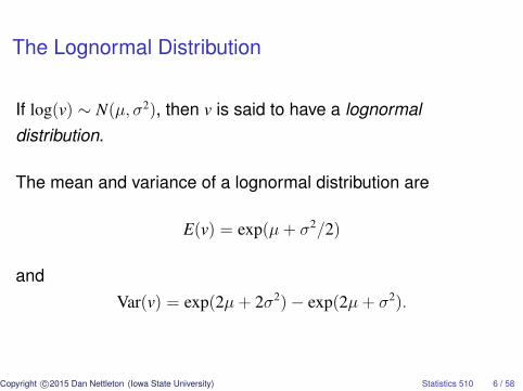
The Lognormal Distribution
If log(v) ∼ N(µ, σ2), then v is said to have a lognormaldistribution.
The mean and variance of a lognormal distribution are
E(v) = exp(µ+ σ2/2)
andVar(v) = exp(2µ+ 2σ2)− exp(2µ+ σ2).
Copyright c©2015 Dan Nettleton (Iowa State University) Statistics 510 6 / 58
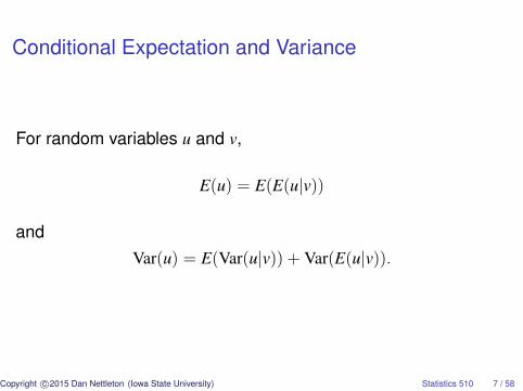
Conditional Expectation and Variance
For random variables u and v,
E(u) = E(E(u|v))
andVar(u) = E(Var(u|v)) + Var(E(u|v)).
Copyright c©2015 Dan Nettleton (Iowa State University) Statistics 510 7 / 58
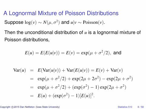
A Lognormal Mixture of Poisson DistributionsSuppose log(v) ∼ N(µ, σ2) and u|v ∼ Poisson(v).
Then the unconditional distribution of u is a lognormal mixture ofPoisson distributions,
E(u) = E(E(u|v)) = E(v) = exp(µ+ σ2/2), and
Var(u) = E(Var(u|v)) + Var(E(u|v)) = E(v) + Var(v)
= exp(µ+ σ2/2) + exp(2µ+ 2σ2)− exp(2µ+ σ2)
= exp(µ+ σ2/2) + (exp(σ2)− 1) exp(2µ+ σ2)
= E(u) + (exp(σ2)− 1)[E(u)]2.
Copyright c©2015 Dan Nettleton (Iowa State University) Statistics 510 8 / 58
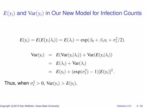
E(yi) and Var(yi) in Our New Model for Infection Counts
E(yi) = E(E(yi|λi)) = E(λi) = exp(β0 + β1xi + σ2`/2).
Var(yi) = E(Var(yi|λi)) + Var(E(yi|λi))
= E(λi) + Var(λi)
= E(yi) + (exp(σ2` )− 1)[E(yi)]
2.
Thus, when σ2` > 0, Var(yi) > E(yi).
Copyright c©2015 Dan Nettleton (Iowa State University) Statistics 510 9 / 58
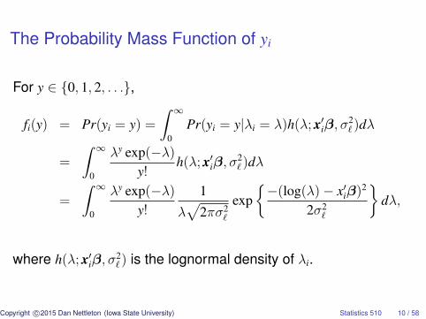
The Probability Mass Function of yi
For y ∈ {0, 1, 2, . . .},
fi(y) = Pr(yi = y) =
∫ ∞0
Pr(yi = y|λi = λ)h(λ; x′iβ, σ2` )dλ
=
∫ ∞0
λy exp(−λ)
y!h(λ; x′iβ, σ
2` )dλ
=
∫ ∞0
λy exp(−λ)
y!
1
λ√
2πσ2`
exp{−(log(λ)− x′iβ)2
2σ2`
}dλ,
where h(λ; x′iβ, σ2` ) is the lognormal density of λi.
Copyright c©2015 Dan Nettleton (Iowa State University) Statistics 510 10 / 58
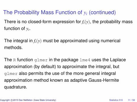
The Probability Mass Function of yi (continued)
There is no closed-form expression for fi(y), the probability massfunction of yi.
The integral in fi(y) must be approximated using numericalmethods.
The R function glmer in the package lme4 uses the Laplaceapproximation (by default) to approximate the integral, butglmer also permits the use of the more general integralapproximation method known as adaptive Gauss-Hermitequadrature.
Copyright c©2015 Dan Nettleton (Iowa State University) Statistics 510 11 / 58
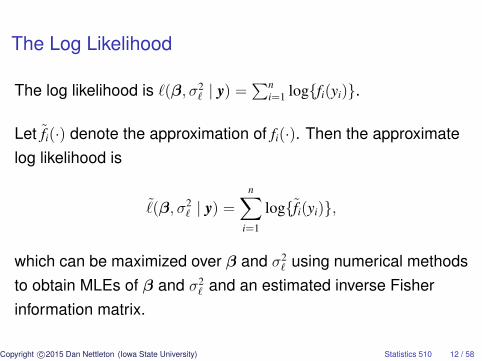
The Log Likelihood
The log likelihood is `(β, σ2` | y) =
∑ni=1 log{fi(yi)}.
Let f̃i(·) denote the approximation of fi(·). Then the approximatelog likelihood is
˜̀(β, σ2` | y) =
n∑i=1
log{f̃i(yi)},
which can be maximized over β and σ2` using numerical methods
to obtain MLEs of β and σ2` and an estimated inverse Fisher
information matrix.
Copyright c©2015 Dan Nettleton (Iowa State University) Statistics 510 12 / 58
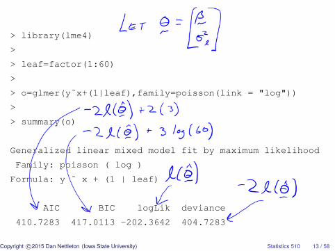
> library(lme4)
>
> leaf=factor(1:60)
>
> o=glmer(y˜x+(1|leaf),family=poisson(link = "log"))
>
> summary(o)
Generalized linear mixed model fit by maximum likelihood
Family: poisson ( log )
Formula: y ˜ x + (1 | leaf)
AIC BIC logLik deviance
410.7283 417.0113 -202.3642 404.7283
Copyright c©2015 Dan Nettleton (Iowa State University) Statistics 510 13 / 58
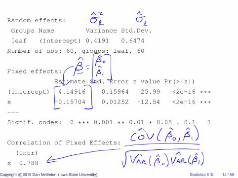
Random effects:
Groups Name Variance Std.Dev.
leaf (Intercept) 0.4191 0.6474
Number of obs: 60, groups: leaf, 60
Fixed effects:
Estimate Std. Error z value Pr(>|z|)
(Intercept) 4.14916 0.15964 25.99 <2e-16 ***
x -0.15704 0.01252 -12.54 <2e-16 ***
---
Signif. codes: 0 *** 0.001 ** 0.01 * 0.05 . 0.1 1
Correlation of Fixed Effects:
(Intr)
x -0.788
Copyright c©2015 Dan Nettleton (Iowa State University) Statistics 510 14 / 58
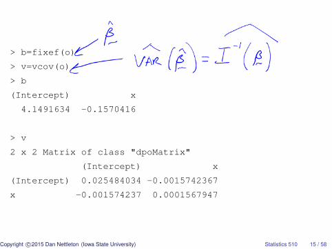
> b=fixef(o)
> v=vcov(o)
> b
(Intercept) x
4.1491634 -0.1570416
> v
2 x 2 Matrix of class "dpoMatrix"
(Intercept) x
(Intercept) 0.025484034 -0.0015742367
x -0.001574237 0.0001567947
Copyright c©2015 Dan Nettleton (Iowa State University) Statistics 510 15 / 58

> sigma.sq.leaf=unlist(VarCorr(o))
>
> sigma.sq.leaf
leaf
0.4191069
Copyright c©2015 Dan Nettleton (Iowa State University) Statistics 510 16 / 58

Conditional vs. Marginal Mean
The conditional mean of yi given `i = 0 is
E(yi|`i = 0) = exp(β0 + β1xi).
The marginal mean of yi is
E(yi) = exp(β0 + β1xi + σ2`/2) = exp(β0 + β1xi) exp(σ2
`/2).
Copyright c©2015 Dan Nettleton (Iowa State University) Statistics 510 17 / 58
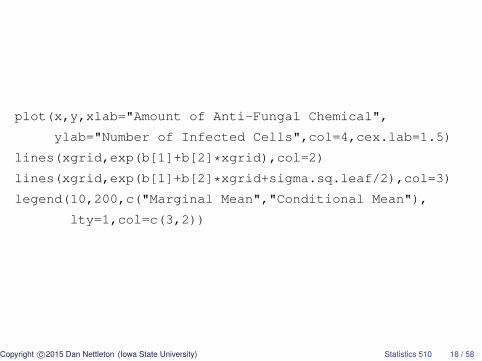
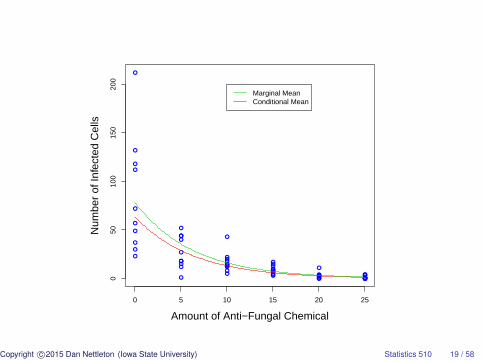
plot(x,y,xlab="Amount of Anti-Fungal Chemical",
ylab="Number of Infected Cells",col=4,cex.lab=1.5)
lines(xgrid,exp(b[1]+b[2]*xgrid),col=2)
lines(xgrid,exp(b[1]+b[2]*xgrid+sigma.sq.leaf/2),col=3)
legend(10,200,c("Marginal Mean","Conditional Mean"),
lty=1,col=c(3,2))
Copyright c©2015 Dan Nettleton (Iowa State University) Statistics 510 18 / 58
●
●
●
●
●
●
●
●
●
●
●●
●
●
●
●
●●
●
●
●●
●
●
●
●
●●●
●●
●
●
●
●
●●●●
● ●
●●●●●●●●● ●●●●
●●●●●●
0 5 10 15 20 25
050
100
150
200
Amount of Anti−Fungal Chemical
Num
ber
of In
fect
ed C
ells
Marginal MeanConditional Mean
Copyright c©2015 Dan Nettleton (Iowa State University) Statistics 510 19 / 58
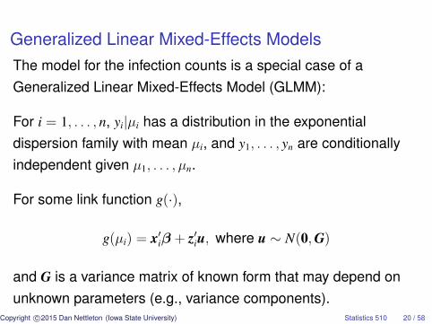
Generalized Linear Mixed-Effects ModelsThe model for the infection counts is a special case of aGeneralized Linear Mixed-Effects Model (GLMM):
For i = 1, . . . , n, yi|µi has a distribution in the exponentialdispersion family with mean µi, and y1, . . . , yn are conditionallyindependent given µ1, . . . , µn.
For some link function g(·),
g(µi) = x′iβ + z′iu, where u ∼ N(0,G)
and G is a variance matrix of known form that may depend onunknown parameters (e.g., variance components).
Copyright c©2015 Dan Nettleton (Iowa State University) Statistics 510 20 / 58

In our model for the infection counts, we have . . .
conditional Poisson distributions,
µi = λi,
g(·) = log(·),
z′i = the ith row of the n× n identity matrix,
u = [`1, . . . , `n]′, and
G = σ2` I.
Copyright c©2015 Dan Nettleton (Iowa State University) Statistics 510 21 / 58
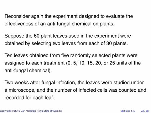
Reconsider again the experiment designed to evaluate theeffectiveness of an anti-fungal chemical on plants.
Suppose the 60 plant leaves used in the experiment wereobtained by selecting two leaves from each of 30 plants.
Ten leaves obtained from five randomly selected plants wereassigned to each treatment (0, 5, 10, 15, 20, or 25 units of theanti-fungal chemical).
Two weeks after fungal infection, the leaves were studied undera microscope, and the number of infected cells was counted andrecorded for each leaf.
Copyright c©2015 Dan Nettleton (Iowa State University) Statistics 510 22 / 58
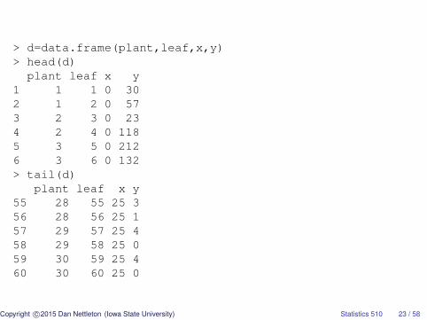
> d=data.frame(plant,leaf,x,y)> head(d)plant leaf x y
1 1 1 0 302 1 2 0 573 2 3 0 234 2 4 0 1185 3 5 0 2126 3 6 0 132> tail(d)
plant leaf x y55 28 55 25 356 28 56 25 157 29 57 25 458 29 58 25 059 30 59 25 460 30 60 25 0
Copyright c©2015 Dan Nettleton (Iowa State University) Statistics 510 23 / 58

An Updated Generalized Linear Mixed-Mixed ModelAll is as in the previous model on slide 5 except that now wehave
log(λi) = x′iβ + z′iu, where
z′i is the ith row of Z = [I30×30 ⊗ 12×1, I60×60] and
u =
p1...p30
`1...`60
∼ N
([00
],
[σ2
pI 00 σ2
` I
]).
Copyright c©2015 Dan Nettleton (Iowa State University) Statistics 510 24 / 58
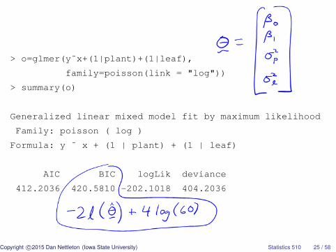
> o=glmer(y˜x+(1|plant)+(1|leaf),
family=poisson(link = "log"))
> summary(o)
Generalized linear mixed model fit by maximum likelihood
Family: poisson ( log )
Formula: y ˜ x + (1 | plant) + (1 | leaf)
AIC BIC logLik deviance
412.2036 420.5810 -202.1018 404.2036
Copyright c©2015 Dan Nettleton (Iowa State University) Statistics 510 25 / 58
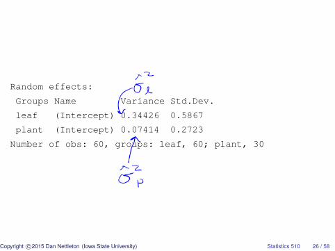
Random effects:
Groups Name Variance Std.Dev.
leaf (Intercept) 0.34426 0.5867
plant (Intercept) 0.07414 0.2723
Number of obs: 60, groups: leaf, 60; plant, 30
Copyright c©2015 Dan Nettleton (Iowa State University) Statistics 510 26 / 58
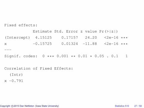
Fixed effects:
Estimate Std. Error z value Pr(>|z|)
(Intercept) 4.15125 0.17157 24.20 <2e-16 ***
x -0.15725 0.01324 -11.88 <2e-16 ***
---
Signif. codes: 0 *** 0.001 ** 0.01 * 0.05 . 0.1 1
Correlation of Fixed Effects:
(Intr)
x -0.791
Copyright c©2015 Dan Nettleton (Iowa State University) Statistics 510 27 / 58
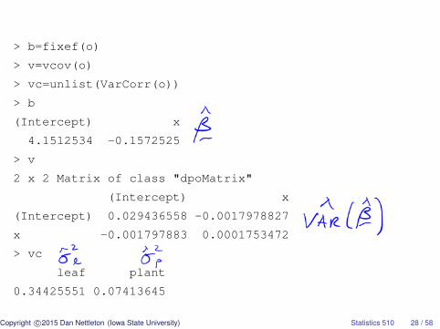
> b=fixef(o)
> v=vcov(o)
> vc=unlist(VarCorr(o))
> b
(Intercept) x
4.1512534 -0.1572525
> v
2 x 2 Matrix of class "dpoMatrix"
(Intercept) x
(Intercept) 0.029436558 -0.0017978827
x -0.001797883 0.0001753472
> vc
leaf plant
0.34425551 0.07413645
Copyright c©2015 Dan Nettleton (Iowa State University) Statistics 510 28 / 58
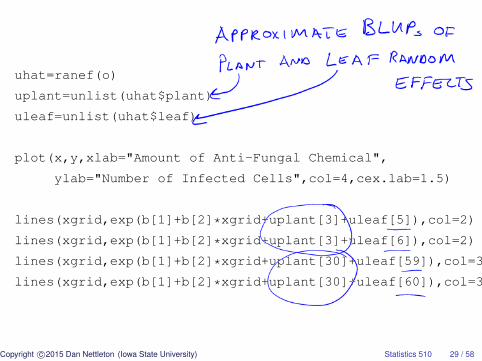
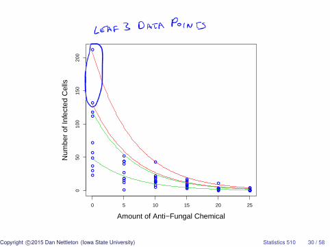
uhat=ranef(o)
uplant=unlist(uhat$plant)
uleaf=unlist(uhat$leaf)
plot(x,y,xlab="Amount of Anti-Fungal Chemical",
ylab="Number of Infected Cells",col=4,cex.lab=1.5)
lines(xgrid,exp(b[1]+b[2]*xgrid+uplant[3]+uleaf[5]),col=2)
lines(xgrid,exp(b[1]+b[2]*xgrid+uplant[3]+uleaf[6]),col=2)
lines(xgrid,exp(b[1]+b[2]*xgrid+uplant[30]+uleaf[59]),col=3)
lines(xgrid,exp(b[1]+b[2]*xgrid+uplant[30]+uleaf[60]),col=3)
Copyright c©2015 Dan Nettleton (Iowa State University) Statistics 510 29 / 58
●
●
●
●
●
●
●
●
●
●
●●
●
●
●
●
●●
●
●
●●
●
●
●
●
●●●
●●
●
●
●
●
●●●●
● ●
●●●●●●●●● ●●●●
●●●●●●
0 5 10 15 20 25
050
100
150
200
Amount of Anti−Fungal Chemical
Num
ber
of In
fect
ed C
ells
Copyright c©2015 Dan Nettleton (Iowa State University) Statistics 510 30 / 58
Now suppose that instead of a conditional Poisson response, wehave a conditional binomial response for each unit in anexperiment or an observational study.
As an example, consider again the trout data set discussed onpage 669 of The Statistical Sleuth, 3rd edition, by Ramsey andSchafer.
Five doses of toxic substance were assigned to a total of 20 fishtanks using a completely randomized design with four tanks perdose.
For each tank, the total number of fish and the number of fishthat developed liver tumors were recorded.
Copyright c©2015 Dan Nettleton (Iowa State University) Statistics 510 31 / 58
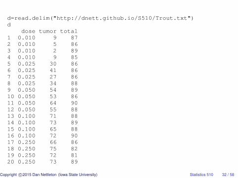
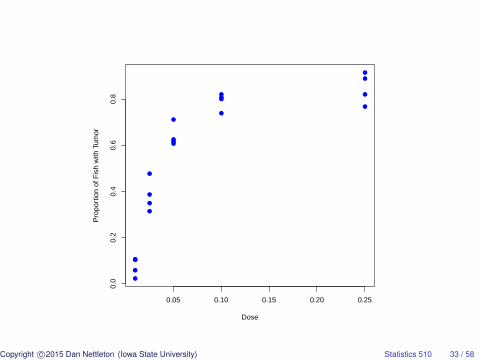
d=read.delim("http://dnett.github.io/S510/Trout.txt")d
dose tumor total1 0.010 9 872 0.010 5 863 0.010 2 894 0.010 9 855 0.025 30 866 0.025 41 867 0.025 27 868 0.025 34 889 0.050 54 8910 0.050 53 8611 0.050 64 9012 0.050 55 8813 0.100 71 8814 0.100 73 8915 0.100 65 8816 0.100 72 9017 0.250 66 8618 0.250 75 8219 0.250 72 8120 0.250 73 89
Copyright c©2015 Dan Nettleton (Iowa State University) Statistics 510 32 / 58
●
●
●
●
●
●
●
●
●●
●
●
●●
●
●
●
●
●
●
0.05 0.10 0.15 0.20 0.25
0.0
0.2
0.4
0.6
0.8
Dose
Pro
port
ion
of F
ish
with
Tum
or
Copyright c©2015 Dan Nettleton (Iowa State University) Statistics 510 33 / 58

A GLMM for the Tumor Data
Let mi = the number of fish in tank i.
Let yi = the proportion of fish in tank i with tumors.
Suppose yi|πiind∼ binomial(mi, πi)/mi.
Then E(yi|πi) = miπi/mi = πi.
Suppose log(
πi1−πi
)= x′iβ + z′iu, where . . .
Copyright c©2015 Dan Nettleton (Iowa State University) Statistics 510 34 / 58
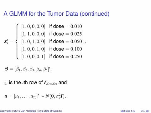
A GLMM for the Tumor Data (continued)
x′i =
[1, 0, 0, 0, 0] if dose = 0.010
[1, 1, 0, 0, 0] if dose = 0.025
[1, 0, 1, 0, 0] if dose = 0.050
[1, 0, 0, 1, 0] if dose = 0.100
[1, 0, 0, 0, 1] if dose = 0.250
,
β = [β1, β2, β3, β4, β5]′,
zi is the ith row of I20×20, and
u = [u1, . . . , u20]′ ∼ N(0, σ2
uI).
Copyright c©2015 Dan Nettleton (Iowa State University) Statistics 510 35 / 58

A GLMM for the Tumor Data (continued)
Alternatively, we could introduce two subscripts (i = 1, 2, 3, 4, 5
for dose and j = 1, 2, 3, 4 for tank nested within dose) and rewritethe same model as
yij|πijind∼ binomial(mij, πij)/mij
log(
πij
1−πij
)= δi + uij
u11, u12, . . . , u53, u54iid∼ N(0, σ2
u)
Copyright c©2015 Dan Nettleton (Iowa State University) Statistics 510 36 / 58
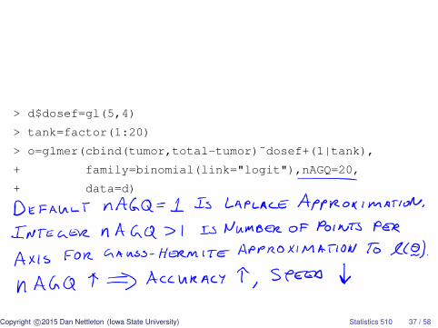
> d$dosef=gl(5,4)
> tank=factor(1:20)
> o=glmer(cbind(tumor,total-tumor)˜dosef+(1|tank),
+ family=binomial(link="logit"),nAGQ=20,
+ data=d)
Copyright c©2015 Dan Nettleton (Iowa State University) Statistics 510 37 / 58
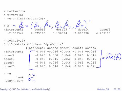
> b=fixef(o)> v=vcov(o)> vc=unlist(VarCorr(o))
> b(Intercept) dosef2 dosef3 dosef4 dosef5-2.559544 2.075196 3.136824 3.896338 4.269113
> round(v,3)5 x 5 Matrix of class "dpoMatrix"
(Intercept) dosef2 dosef3 dosef4 dosef5(Intercept) 0.046 -0.046 -0.046 -0.046 -0.046dosef2 -0.046 0.060 0.046 0.046 0.046dosef3 -0.046 0.046 0.060 0.046 0.046dosef4 -0.046 0.046 0.046 0.065 0.046dosef5 -0.046 0.046 0.046 0.046 0.071
> vctank
0.009590674
Copyright c©2015 Dan Nettleton (Iowa State University) Statistics 510 38 / 58
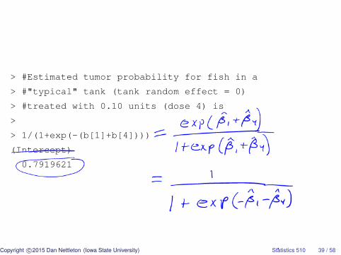
> #Estimated tumor probability for fish in a
> #"typical" tank (tank random effect = 0)
> #treated with 0.10 units (dose 4) is
>
> 1/(1+exp(-(b[1]+b[4])))
(Intercept)
0.7919621
Copyright c©2015 Dan Nettleton (Iowa State University) Statistics 510 39 / 58
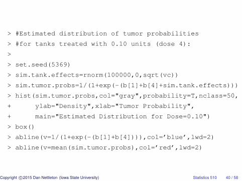
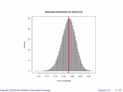
> #Estimated distribution of tumor probabilities
> #for tanks treated with 0.10 units (dose 4):
>
> set.seed(5369)
> sim.tank.effects=rnorm(100000,0,sqrt(vc))
> sim.tumor.probs=1/(1+exp(-(b[1]+b[4]+sim.tank.effects)))
> hist(sim.tumor.probs,col="gray",probability=T,nclass=50,
+ ylab="Density",xlab="Tumor Probability",
+ main="Estimated Distribution for Dose=0.10")
> box()
> abline(v=1/(1+exp(-(b[1]+b[4]))),col=’blue’,lwd=2)
> abline(v=mean(sim.tumor.probs),col=’red’,lwd=2)
Copyright c©2015 Dan Nettleton (Iowa State University) Statistics 510 40 / 58
Estimated Distribution for Dose=0.10
Tumor Probability
Den
sity
0.72 0.74 0.76 0.78 0.80 0.82 0.84
05
1015
2025
Copyright c©2015 Dan Nettleton (Iowa State University) Statistics 510 41 / 58
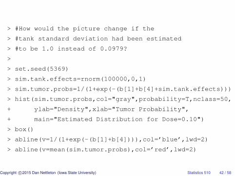
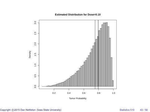
> #How would the picture change if the
> #tank standard deviation had been estimated
> #to be 1.0 instead of 0.0979?
>
> set.seed(5369)
> sim.tank.effects=rnorm(100000,0,1)
> sim.tumor.probs=1/(1+exp(-(b[1]+b[4]+sim.tank.effects)))
> hist(sim.tumor.probs,col="gray",probability=T,nclass=50,
+ ylab="Density",xlab="Tumor Probability",
+ main="Estimated Distribution for Dose=0.10")
> box()
> abline(v=1/(1+exp(-(b[1]+b[4]))),col=’blue’,lwd=2)
> abline(v=mean(sim.tumor.probs),col=’red’,lwd=2)
Copyright c©2015 Dan Nettleton (Iowa State University) Statistics 510 42 / 58
Estimated Distribution for Dose=0.10
Tumor Probability
Den
sity
0.2 0.4 0.6 0.8 1.0
0.0
0.5
1.0
1.5
2.0
2.5
3.0
Copyright c©2015 Dan Nettleton (Iowa State University) Statistics 510 43 / 58
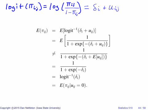
E(πij) = E[logit−1(δi + uij)]
= E[
11 + exp{−(δi + uij)}
]6= 1
1 + exp{−(δi + E[uij])}
=1
1 + exp(−δi)
= logit−1(δi)
= E(πij|uij = 0).
Copyright c©2015 Dan Nettleton (Iowa State University) Statistics 510 44 / 58
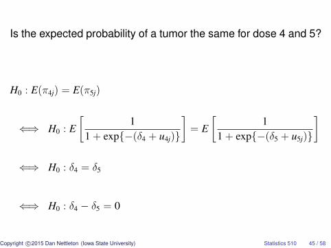
Is the expected probability of a tumor the same for dose 4 and 5?
H0 : E(π4j) = E(π5j)
⇐⇒ H0 : E[
11 + exp{−(δ4 + u4j)}
]= E
[1
1 + exp{−(δ5 + u5j)}
]
⇐⇒ H0 : δ4 = δ5
⇐⇒ H0 : δ4 − δ5 = 0
Copyright c©2015 Dan Nettleton (Iowa State University) Statistics 510 45 / 58

Test of H0 : δ4 − δ5 = 0
> cc=c(0,0,0,1,-1)
> est=drop(t(cc)%*%b)
> est
[1] -0.372775
> se=drop(sqrt(t(cc)%*%v%*%cc))
> z.stat=est/se
> z.stat
[1] -1.763663
> p.value=2*(1-pnorm(abs(z.stat),0,1))
> p.value
[1] 0.07778872
Copyright c©2015 Dan Nettleton (Iowa State University) Statistics 510 46 / 58
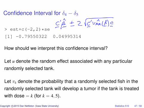
Confidence Interval for δ4 − δ5
> est+c(-2,2)*se
[1] -0.79550322 0.04995314
How should we interpret this confidence interval?
Let u denote the random effect associated with any particularrandomly selected tank.
Let πk denote the probability that a randomly selected fish in therandomly selected tank will develop a tumor if the tank is treatedwith dose = k (for k = 4, 5).
Copyright c©2015 Dan Nettleton (Iowa State University) Statistics 510 47 / 58

Our model says log(
π41−π4
)= δ4 + u and log
(π5
1−π5
)= δ5 + u.
Thus,
δ4 − δ5 = (δ4 + u)− (δ5 + u)
= log(
π4
1− π4
)− log
(π5
1− π5
)= log
(π4
1− π4
/π5
1− π5
),
which implies π51−π5
= exp(δ5 − δ4)π4
1−π4.
Copyright c©2015 Dan Nettleton (Iowa State University) Statistics 510 48 / 58
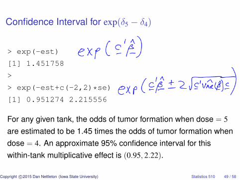
Confidence Interval for exp(δ5 − δ4)
> exp(-est)
[1] 1.451758
>
> exp(-est+c(-2,2)*se)
[1] 0.951274 2.215556
For any given tank, the odds of tumor formation when dose = 5
are estimated to be 1.45 times the odds of tumor formation whendose = 4. An approximate 95% confidence interval for thiswithin-tank multiplicative effect is (0.95, 2.22).
Copyright c©2015 Dan Nettleton (Iowa State University) Statistics 510 49 / 58
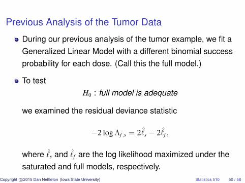
Previous Analysis of the Tumor Data
During our previous analysis of the tumor example, we fit aGeneralized Linear Model with a different binomial successprobability for each dose. (Call this the full model.)
To testH0 : full model is adequate
we examined the residual deviance statistic
−2 log Λf ,s = 2ˆ̀s − 2ˆ̀
f ,
where ˆ̀s and ˆ̀
f are the log likelihood maximized under thesaturated and full models, respectively.
Copyright c©2015 Dan Nettleton (Iowa State University) Statistics 510 50 / 58

Previous Analysis of the Tumor Data (continued)
The residual deviance statistic −2 log Λf ,s = 2ˆ̀s − 2ˆ̀
f isapproximately distributed as χ2
n−pfunder H0, where n = 20 is
the dimension of the saturated model parameter space andpf = 5 is the dimension of the full model parameter space.
Because the observed value of −2 log Λf ,s = 2ˆ̀s − 2ˆ̀
f wasunusually large for a χ2
n−pfrandom variable, we detected lack
of fit.
If the lack of fit is due to overdispersion, we now have twodifferent strategies for managing overdispersion.
Copyright c©2015 Dan Nettleton (Iowa State University) Statistics 510 51 / 58
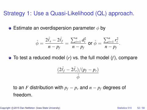
Strategy 1: Use a Quasi-Likelihood (QL) approach.
Estimate an overdispersion parameter φ by
φ̂ =2ˆ̀
s − 2ˆ̀f
n− pf=
∑ni=1 d2
i
n− pfor φ̂ =
∑ni=1 r2
i
n− pf.
To test a reduced model (r) vs. the full model (f ), compare
(2ˆ̀f − 2ˆ̀
r)/(pf − pr)
φ̂
to an F distribution with pf − pr and n− pf degrees offreedom.
Copyright c©2015 Dan Nettleton (Iowa State University) Statistics 510 52 / 58
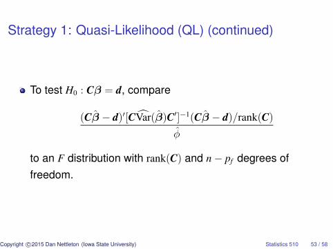
Strategy 1: Quasi-Likelihood (QL) (continued)
To test H0 : Cβ = d, compare
(Cβ̂ − d)′[CV̂ar(β̂)C′]−1(Cβ̂ − d)/rank(C)
φ̂
to an F distribution with rank(C) and n− pf degrees offreedom.
Copyright c©2015 Dan Nettleton (Iowa State University) Statistics 510 53 / 58
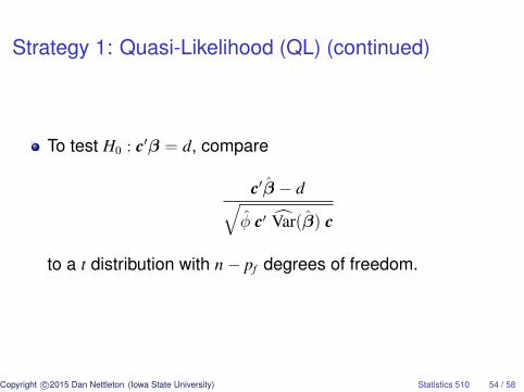
Strategy 1: Quasi-Likelihood (QL) (continued)
To test H0 : c′β = d, compare
c′β̂ − d√φ̂ c′ V̂ar(β̂) c
to a t distribution with n− pf degrees of freedom.
Copyright c©2015 Dan Nettleton (Iowa State University) Statistics 510 54 / 58
Strategy 1: Quasi-Likelihood (QL) (continued)
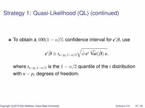
To obtain a 100(1− α)% confidence interval for c′β, use
c′β̂ ± tn−pf ,1−α/2
√φ̂ c′ V̂ar(β̂) c,
where tn−pf ,1−α/2 is the 1− α/2 quantile of the t distributionwith n− pf degrees of freedom.
Copyright c©2015 Dan Nettleton (Iowa State University) Statistics 510 55 / 58
Strategy 1: Quasi-Likelihood (QL) (continued)
If you use a QL approach, you are not fitting a new model.
Rather, you are adjusting the inference strategy to accountfor overdispersion in the data relative to the original fullmodel you fit.
There is no point in re-testing for overdispersion once youdecide to use the QL inference strategy.
Data are still overdispersed relative to the fitted model, butthe QL inference strategy adjusts for overdispersion to gettests with approximately the right size and confidenceintervals with closer to nominal coverage rates (in theory).
Copyright c©2015 Dan Nettleton (Iowa State University) Statistics 510 56 / 58
Strategy 2: Fit a GLMM
A GLMM with a random effect for each observation is onenatural model for overdispersed data.
We do not re-test for overdispersion once we decide to usea GLMM with a random effect for each observation becausethe model we are fitting allows for overdispersed data.
Because GLMM inference relies on asymptotic normal andchi-square approximations, it may be more liberal (p-valuessmaller and confidence intervals narrower) than the QLapproach, especially for small datasets.
Copyright c©2015 Dan Nettleton (Iowa State University) Statistics 510 57 / 58
Another Reason for Choosing a GLMM
In the last description of the experiment to study the effectsof an anti-fungal chemical, plants are the experimental unitsand leaves are the observational units.
As was the case for experiments with normally distributedresponses, a random effect for each experimental unitshould be included in a model for the data when there ismore than one observation per experimental unit.
In the model for the infection count data, the plant randomeffects allow for correlation between the responses of leavesfrom the same plant.
Copyright c©2015 Dan Nettleton (Iowa State University) Statistics 510 58 / 58