STAT 705 Generalized linear mixed models

Timothy Hanson

Department of Statistics, University of South Carolina

Stat 705: Data Analysis II

1 / 24

Generalized Linear Mixed Models

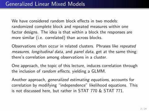
We have considered random block effects in two models:randomized complete block and repeated measures within onefactor designs. The idea is that within a block the responses aremore similar (i.e. correlated) than across blocks.

Observations often occur in related clusters. Phrases like repeatedmeasures, longitudinal data, and panel data, get at the same thing:there’s correlation among observations in a cluster.

One approach, the topic of this lecture, induces correlation throughthe inclusion of random effects, yielding a GLMM.

Another approach, generalized estimating equations, accounts forcorrelation by modifying “independence” likelihood equations. Thisis not discussed here, but rather in STAT 770 & STAT 771.

2 / 24

Add random effects to linear predictor

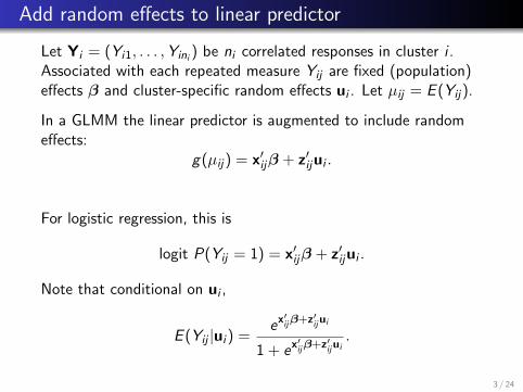
Let Yi = (Yi1, . . . ,Yini) be ni correlated responses in cluster i .

Associated with each repeated measure Yij are fixed (population)effects β and cluster-specific random effects ui . Let µij = E (Yij).

In a GLMM the linear predictor is augmented to include randomeffects:

g(µij) = x′ijβ + z′ijui .

For logistic regression, this is

logit P(Yij = 1) = x′ijβ + z′ijui .

Note that conditional on ui ,

E (Yij |ui ) =ex′ijβ+z′ij ui

1 + ex′ijβ+z′ij ui.

3 / 24

Example

I ask a random sample of the same n = 14 STAT 705 graduatestudents “do you like statistics?” once a month for 4 months.

Yij = 1 if “yes” and Yij = 0 if no. Here, i = 1, . . . , 14 andj = 1, . . . , 4.

Covariates might include mij , the average mood of the studentover the previous month (mij = 0 is bad, mij = 1 is good), thedegree being sought (di = 0 doctoral, di = 1 masters), the monthtj = j , and pj the number of homework problems assigned in STAT705 in the previous month.

A GLMM might be

logit P(Yij = 1) = β0 + β1mij + β2di + β3pj + β4j + ui .

This model assumes that log-odds of liking statistics changeslinearly in time, holding all else constant. Alternatively, we mightfit a quadratic instead or treat time as categorical. Here, ui

represents a student’s a priori disposition towards statistics.4 / 24

Interpretation

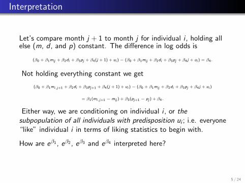
Let’s compare month j + 1 to month j for individual i , holding allelse (m, d , and p) constant. The difference in log odds is

(β0 + β1mij + β2di + β3pj + β4(j + 1) + ui )− (β0 + β1mij + β2di + β3pj + β4j + ui ) = β4.

Not holding everything constant we get

(β0 + β1mi,j+1 + β2di + β3pj+1 + β4(j + 1) + ui )− (β0 + β1mij + β2di + β3pj + β4j + ui )

= β1(mi,j+1 − mij ) + β3(pj+1 − pj ) + β4.

Either way, we are conditioning on individual i , or thesubpopulation of all individuals with predisposition ui ; i.e. everyone“like” individual i in terms of liking statistics to begin with.

How are eβ1 , eβ2 , eβ3 and eβ4 interpreted here?

5 / 24

Random effects u1, . . . , un

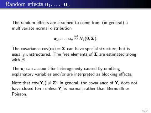
The random effects are assumed to come from (in general) amultivariate normal distribution

u1, . . . ,uniid∼ Nq(0,Σ).

The covariance cov(ui ) = Σ can have special structure, but isusually unstructured. The free elements of Σ are estimated alongwith β.

The ui can account for heterogeneity caused by omittingexplanatory variables and/or are interpreted as blocking effects.

Note that cov(Yi ) 6= Σ! In general, the covariance of Yi does nothave closed form unless Yi is normal, rather than Bernoulli orPoisson.

6 / 24

Two special cases

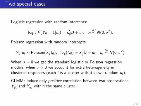
Logistic regression with random intercepts:

logit P(Yij = 1|ui ) = x′ijβ + ui , uiiid∼ N(0, σ2).

Poisson regression with random intercepts:

Yij |ui ∼ Poisson(λij tij), log(λij) = x′ijβ + ui , uiiid∼ N(0, σ2).

When σ = 0 we get the standard logistic or Poisson regressionmodels; when σ > 0 we account for extra heterogeneity inclustered responses (each i is a cluster with it’s own random ui ).

GLMMs induce only positive correlation between two observationsYij1 and Yij2 within the same cluster.

7 / 24

Fitting binary GLMMs

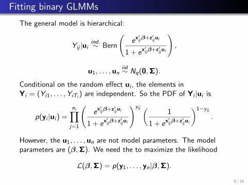
The general model is hierarchical:

Yij |uiind .∼ Bern

(ex′ijβ+z′ij ui

1 + ex′ijβ+z′ij ui

),

u1, . . . ,uniid∼ Nq(0,Σ).

Conditional on the random effect ui , the elements inYi = (Yi1, . . . ,YiTi

) are independent. So the PDF of Yi |ui is

p(yi |ui ) =

ni∏j=1

(ex′ijβ+z′ij ui

1 + ex′ijβ+z′ij ui

)yij (1

1 + ex′ijβ+z′ij ui

)1−yij

.

However, the u1, . . . ,un are not model parameters. The modelparameters are (β,Σ). We need the to maximize the likelihood

L(β,Σ) = p(y1, . . . , yn|β,Σ).

8 / 24

Integrate to get likelihood

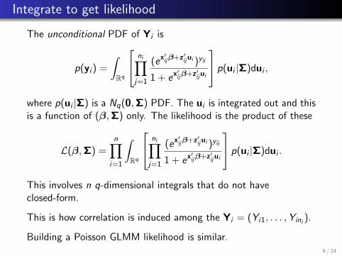
The unconditional PDF of Yi is

p(yi ) =

∫Rq

ni∏j=1

(ex′ijβ+z′ij ui )yij

1 + ex′ijβ+z′ij ui

p(ui |Σ)dui ,

where p(ui |Σ) is a Nq(0,Σ) PDF. The ui is integrated out and thisis a function of (β,Σ) only. The likelihood is the product of these

L(β,Σ) =n∏

i=1

∫Rq

ni∏j=1

(ex′ijβ+z′ij ui )yij

1 + ex′ijβ+z′ij ui

p(ui |Σ)dui .

This involves n q-dimensional integrals that do not haveclosed-form.

This is how correlation is induced among the Yi = (Yi1, . . . ,Yini).

Building a Poisson GLMM likelihood is similar.9 / 24

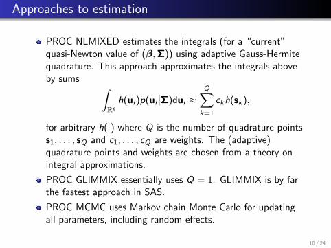
Approaches to estimation

PROC NLMIXED estimates the integrals (for a “current”quasi-Newton value of (β,Σ)) using adaptive Gauss-Hermitequadrature. This approach approximates the integrals aboveby sums ∫

Rq

h(ui )p(ui |Σ)dui ≈Q∑

k=1

ckh(sk),

for arbitrary h(·) where Q is the number of quadrature pointss1, . . . , sQ and c1, . . . , cQ are weights. The (adaptive)quadrature points and weights are chosen from a theory onintegral approximations.

PROC GLIMMIX essentially uses Q = 1. GLIMMIX is by farthe fastest approach in SAS.

PROC MCMC uses Markov chain Monte Carlo for updatingall parameters, including random effects.

10 / 24

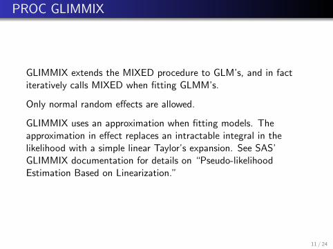
PROC GLIMMIX

GLIMMIX extends the MIXED procedure to GLM’s, and in factiteratively calls MIXED when fitting GLMM’s.

Only normal random effects are allowed.

GLIMMIX uses an approximation when fitting models. Theapproximation in effect replaces an intractable integral in thelikelihood with a simple linear Taylor’s expansion. See SAS’GLIMMIX documentation for details on “Pseudo-likelihoodEstimation Based on Linearization.”

11 / 24

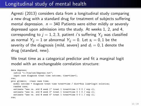
Longitudinal study of mental health

Agresti (2013) considers data from a longitudinal study comparinga new drug with a standard drug for treatment of subjects sufferingmental depression. n = 340 Patients were either mildly or severelydepressed upon admission into the study. At weeks 1, 2, and 4,corresponding to j = 1, 2, 3, patient i ’s suffering Yij was classifiedas normal Yij = 1 or abnormal Yij = 0. Let si = 0, 1 be theseverity of the diagnosis (mild, severe) and di = 0, 1 denote thedrug (standard, new).

We treat time as a categorical predictor and fit a marginal logitmodel with an exchangeable correlation structure:

data depress;

infile "c:/tim/cat/depress.txt";

input case diagnose treat time outcome; time=time+1;

run;

proc glimmix; class case time;

model outcome = diagnose treat time treat*time / dist=bin link=logit solution;

random case;

estimate "new vs. std @ week 1" treat 1 treat*time 1 0 0 / exp cl;

estimate "new vs. std @ week 2" treat 1 treat*time 0 1 0 / exp cl;

estimate "new vs. std @ week 4" treat 1 treat*time 0 0 1 / exp cl;

run;

12 / 24

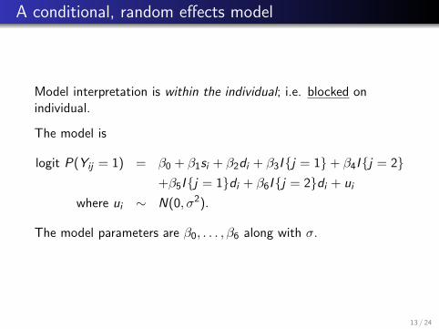
A conditional, random effects model

Model interpretation is within the individual; i.e. blocked onindividual.

The model is

logit P(Yij = 1) = β0 + β1si + β2di + β3I{j = 1}+ β4I{j = 2}+β5I{j = 1}di + β6I{j = 2}di + ui

where ui ∼ N(0, σ2).

The model parameters are β0, . . . , β6 along with σ.

13 / 24

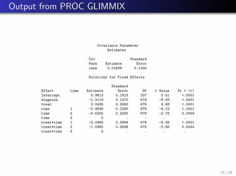
Output from PROC GLIMMIX

Covariance Parameter

Estimates

Cov Standard

Parm Estimate Error

case 0.01838 0.1330

Solutions for Fixed Effects

Standard

Effect time Estimate Error DF t Value Pr > |t|

Intercept 0.9813 0.1813 337 5.41 <.0001

diagnose -1.3119 0.1470 676 -8.93 <.0001

treat 2.0435 0.3060 676 6.68 <.0001

time 1 -0.9599 0.2290 676 -4.19 <.0001

time 2 -0.6205 0.2245 676 -2.76 0.0059

time 3 0 . . . .

treat*time 1 -2.0989 0.3894 676 -5.39 <.0001

treat*time 2 -1.0965 0.3838 676 -2.86 0.0044

treat*time 3 0 . . . .

14 / 24

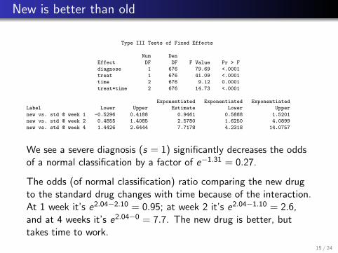
New is better than old

Type III Tests of Fixed Effects

Num Den

Effect DF DF F Value Pr > F

diagnose 1 676 79.69 <.0001

treat 1 676 41.09 <.0001

time 2 676 9.12 0.0001

treat*time 2 676 14.73 <.0001

Exponentiated Exponentiated Exponentiated

Label Lower Upper Estimate Lower Upper

new vs. std @ week 1 -0.5296 0.4188 0.9461 0.5888 1.5201

new vs. std @ week 2 0.4855 1.4085 2.5780 1.6250 4.0899

new vs. std @ week 4 1.4426 2.6444 7.7178 4.2318 14.0757

We see a severe diagnosis (s = 1) significantly decreases the oddsof a normal classification by a factor of e−1.31 = 0.27.

The odds (of normal classification) ratio comparing the new drugto the standard drug changes with time because of the interaction.At 1 week it’s e2.04−2.10 = 0.95; at week 2 it’s e2.04−1.10 = 2.6,and at 4 weeks it’s e2.04−0 = 7.7. The new drug is better, buttakes time to work.

15 / 24

Ache monkey hunting

Data on the number of capuchin monkeys killed by 47 Achehunters over several hunting trips were recorded. There were 363total records. Recall that monkey hunting involves splitting intogroups, chasing monkeys through the trees, and shooting arrowsstraight up.

Let Yij be the number of monkey’s killed by hunter i , i = 1, . . . , 47on trip j of length Lij (the trip length serves as an ‘offset’ in themodel fitting). Let λi be the hunter i ’s kill rate (per day).

Yij ∼ Poisson(λiLij),

wherelog λi = β0 + β1ai + β2a2

i + ui ,

u1, . . . , u47iid∼ N(0, σ2).

16 / 24

Monkey hunting

We include a quadratic effect because we expect a “leveling off”effect or possible decline in ability with age.

Of interest is when hunting ability is greatest. Hunting prowesscontributes to a man’s status within the group. ai is hunter i ’sage-45 years.

An individual’s kill rate is given by λ = eβ0+β1a+β2a2eu, where a is

the individual’s age and u is their latent hunting ability, i.e. theirblocking effect.

One can compare the effect of age within the span of, say, 20 to60 years, to the spread of eu to see which explains more of thevariability in terms of hunting ability: age or innate ability.

17 / 24

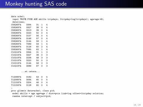
Monkey hunting SAS code

data ache1;

input TRIP$ PID$ AGE nkills tripdays; ltripday=log(tripdays); age=age-45;

datalines;

C082697A 3394 31 1 4

C082697A 3327 38 0 4

C082697A 3313 39 0 4

C082697A 3220 50 0 4

C082697A 3157 56 0 4

C082697A 3146 57 0 4

C082697A 3144 58 1 4

C082697A 7089 59 1 4

C082697A 3126 60 2 4

C082697A 7085 62 1 4

C102197A 3394 31 1 3

C102197A 3327 38 0 3

C102197A 3238 48 3 3

C102197A 3220 50 0 3

C102197A 3144 58 2 3

C102197A 3086 67 0 3

...et cetera...

T120997A 3182 53 0 5

T120997A 3094 65 0 5

T121597A 3254 46 0 4

T121597A 3128 60 0 4

;

proc glimmix data=ache1; class pid;

model nkills = age age*age / dist=pois link=log offset=ltripday solution;

random intercept / subject=pid;

18 / 24

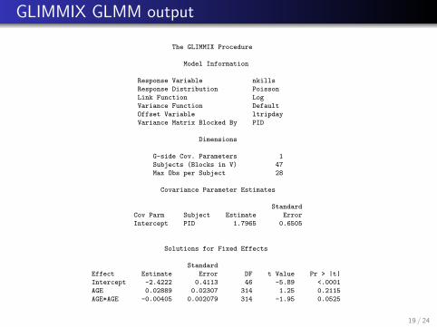
GLIMMIX GLMM output

The GLIMMIX Procedure

Model Information

Response Variable nkills

Response Distribution Poisson

Link Function Log

Variance Function Default

Offset Variable ltripday

Variance Matrix Blocked By PID

Dimensions

G-side Cov. Parameters 1

Subjects (Blocks in V) 47

Max Obs per Subject 28

Covariance Parameter Estimates

Standard

Cov Parm Subject Estimate Error

Intercept PID 1.7965 0.6505

Solutions for Fixed Effects

Standard

Effect Estimate Error DF t Value Pr > |t|

Intercept -2.4222 0.4113 46 -5.89 <.0001

AGE 0.02889 0.02307 314 1.25 0.2115

AGE*AGE -0.00405 0.002079 314 -1.95 0.0525

19 / 24

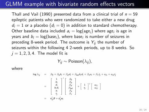
GLMM example with bivariate random effects vectors

Thall and Vail (1990) presented data from a clinical trial of n = 59epileptic patients who were randomized to take either a new drugdi = 1 or a placebo (di = 0) in addition to standard chemotherapy.Other baseline data included ai = log(agei ) where agei is age inyears and bi = log(basei ), where basei is number of seizures inpreceding 8-week period. The outcome is Yij the number ofseizures within the following 4 2-week periods, up to 8 weeks. Soj = 1, 2, 3, 4. The model fit is

Yij ∼ Poisson(λij),

wherelog λij = β0 + βbbi + βddi + βbdbi di + βaai + βv tj + ui1 + ui2tj

=

1bidi

bi diaitj

′

β0βbβdβbdβaβv

+

[1tj

]′ [ ui1ui2

]

= x′ij β + z′ij ui

20 / 24

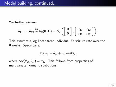
Model building, continued...

We further assume

u1, . . . ,u59iid∼ N2(0,Σ) = N2

([00

],

[σ11 σ12

σ12 σ22

]).

This assumes a log linear trend individual i ’s seizure rate over the8 weeks. Specifically,

log λij = θ0i + θ1iweeksj ,

where cov(θ0i , θ1i ) = σ12. This follows from properties ofmultivariate normal distributions.

21 / 24

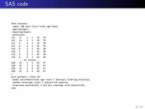
SAS code

data seizure;

input id$ seiz visit treat age base;

age=log(age);

base=log(base);

datalines;

101 11 1 1 18 76

101 14 2 1 18 76

101 9 3 1 18 76

101 8 4 1 18 76

102 8 1 1 32 38

102 7 2 1 32 38

102 9 3 1 32 38

102 4 4 1 32 38

...et cetera...

238 13 1 0 22 47

238 15 2 0 22 47

238 13 3 0 22 47

238 12 4 0 22 47

;

proc glimmix; class id;

model seiz=base|treat age visit / dist=poi link=log solution;

random intercept visit / subject=id type=un;

nloptions maxiter=50; * did not converge with default=20;

run;

22 / 24

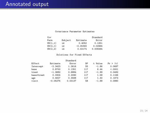
Annotated output

Covariance Parameter Estimates

Cov Standard

Parm Subject Estimate Error

UN(1,1) id 0.4052 0.1251

UN(2,1) id -0.05393 0.02964

UN(2,2) id 0.02174 0.009264

Solutions for Fixed Effects

Standard

Effect Estimate Error DF t Value Pr > |t|

Intercept -2.3423 1.2616 55 -1.86 0.0687

base 0.8700 0.1351 117 6.44 <.0001

treat -1.3682 0.6884 117 -1.99 0.0492

base*treat 0.3304 0.2090 117 1.58 0.1166

age 0.4627 0.3568 117 1.30 0.1973

visit -0.05276 0.03137 58 -1.68 0.0980

23 / 24

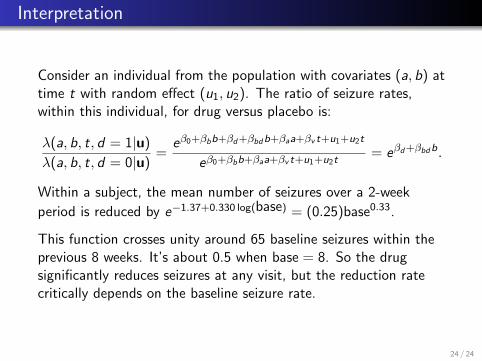
Interpretation

Consider an individual from the population with covariates (a, b) attime t with random effect (u1, u2). The ratio of seizure rates,within this individual, for drug versus placebo is:

λ(a, b, t, d = 1|u)

λ(a, b, t, d = 0|u)=

eβ0+βbb+βd+βbdb+βaa+βv t+u1+u2t

eβ0+βbb+βaa+βv t+u1+u2t= eβd+βbdb.

Within a subject, the mean number of seizures over a 2-week

period is reduced by e−1.37+0.330 log(base) = (0.25)base0.33.

This function crosses unity around 65 baseline seizures within theprevious 8 weeks. It’s about 0.5 when base = 8. So the drugsignificantly reduces seizures at any visit, but the reduction ratecritically depends on the baseline seizure rate.

24 / 24