geographic smoothing of solar pv: results from gujarat · 2019-10-07 · geographic smoothing of...
TRANSCRIPT

Carnegie Mellon Electricity Industry Center Working Paper CEIC-15-03 www.cmu.edu/electricity
DO NOT CITE OR QUOTE WITHOUT THE PERMISSION OF THE AUTHORS 1
Geographic smoothing of solar PV: Results from Gujarat Kelly Klima†,* Jay Apt†, ‡ May 6, 2015 †Department of Engineering and Public Policy, Carnegie Mellon University, 5000 Forbes Avenue, Pittsburgh, PA 15213, USA ‡Tepper School of Business, Carnegie Mellon University, 5000 Forbes Avenue, Pittsburgh, PA 15213, USA * Corresponding Author: [email protected]; 412-268-3705 Short Title: Geographic smoothing of solar PV Keywords: solar photovoltaic, geographic smoothing

Carnegie Mellon Electricity Industry Center Working Paper CEIC-15-03 www.cmu.edu/electricity
DO NOT CITE OR QUOTE WITHOUT THE PERMISSION OF THE AUTHORS 2
Abstract We examine the potential for geographic smoothing of solar photovoltaic (PV) electricity generation using 13 months of observed power production from utility-scale plants in Gujarat, India. To our knowledge, this is the first published analysis of geographic smoothing of solar PV using actual generation data at high time resolution from utility-scale solar PV plants. We use geographic correlation and Fourier transform estimates of the power spectral density (PSD) to characterize the observed variability of operating solar PV plants as a function of time scale. Most plants show a spectrum that is linear in the loglog domain at high frequencies f, ranging from f-1.23 to f-1.56 (slopes of -1.23 and -1.56), thus exhibiting more relative variability at high frequencies than exhibited by wind plants. PSDs for large PV plants have a steeper slope than those for small plants, hence more smoothing at short time scales. Interconnecting 20 Gujarat plants yields a f-1.66 spectrum, reducing fluctuations at frequencies corresponding to 6 hours and 1 hour by 23% and 45%, respectively. Half this smoothing can be obtained through connecting 4-5 plants; the diminishing returns of less than 1% occurs at 12-14 plants. The largest plant (322MW) showed an f-1.76 spectrum. This suggests that in Gujarat, the potential for smoothing is limited to that obtained by one large plant.
Carnegie Mellon Electricity Industry Center Working Paper CEIC-15-03 www.cmu.edu/electricity
DO NOT CITE OR QUOTE WITHOUT THE PERMISSION OF THE AUTHORS 3
1. Introduction Low-pollution electric power sources, such as solar power, have significant potential to reduce the emissions associated with generating electricity. However, solar photovoltaic (PV) generation is a variable energy source, with large and rapid changes in output [1, 2]. This variability of solar PV is sometimes cited as a barrier to its large scale integration into the grid [3, 4, 5, 6]. Many authors have examined the potential for geographic smoothing of PV in the time domain. That literature is of two broad types. One uses modeled or (less commonly) measured solar illumination. The second uses observed data from power plants. There are few of the second type because data are often proprietary and unavailable to researchers. Here we use 13 months of approximately 1- or 2-minute time resolution data from 50 utility-scale PV plants separated by up to 470 km; we have made these data publically available. Some hope that geographic separation may smooth PV variability comes from irradiance studies. The correlation of solar irradiance measured at two locations decreases as the distance between the sites increases [7, 8, 9, 10, 11, 12, 13, 14]. In addition, cloud models have been used to estimate the smoothing effect of geographic diversity [15, 16], and changes in clear sky index for twenty-three locations show smoothing is likely for as few as five plants [2]. However, studies examining actual generation data provide conflicting results. Five-minute step changes in normalized PV power from one German plant can exceed +/-50% but are never larger than +/- 5% for 100 summed German PV sites [17]. Modeled generation at hourly resolution shows smoothing, which is greater on partly-cloudy days [18]. Other studies have examined area effects, suggesting that larger capacity plants [19, 20] or plants spread out over a wider area [21] exhibit less variability than smaller or more densely packed solar farms, respectively. Similarly, geographic smoothing using a large number of smaller plants can reduce variability [22, 23, 24, 25], where the maximum variability is theoretically proportional to the square root of the number of plants aggregated [26]. On the other hand, several studies suggest smoothing may not occur. For instance, correlation of real power output for three tracking PV sites in Arizona is high, suggesting smoothing might not be effective there [1]. Similarly, Murata et al. find that sites in Japan separated by less than about 200 km are not independent [27],which suggests smoothing might also not be effective there. Here we examine the potential for geographic smoothing of solar PV in the Indian state of Gujarat using actual generation data from multiple utility-scale solar power installations. We use geographic correlation and Fourier transform techniques to estimate the power spectral density (PSD) [28, 29] and characterize the observed variability of operating solar PV plants as a function of time scale.
Carnegie Mellon Electricity Industry Center Working Paper CEIC-15-03 www.cmu.edu/electricity
DO NOT CITE OR QUOTE WITHOUT THE PERMISSION OF THE AUTHORS 4
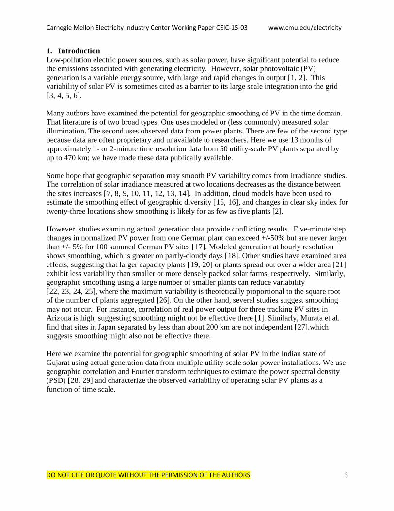
Figure 1: Generation data for the Precious Energy’s 15 MW plant (Plant 5 in the listing in the Supplementary Data) for a) a year, b) a week, c) a clear day, and d) a partly-cloudy day.
2. Data Real time generation data from the State Load Dispatch Centre of Gujarat Energy Transmission Corporation website are available [30] for fifty solar PV plants in Gujarat, India. These measured power output values are updated at uneven time intervals, generally ranging between one to two minutes. We captured website data at one-minute intervals from February 17, 2014 to March 16, 2015. The data capture process, link to our archived data, and power plant characteristics are in the Supplementary Data. We used four tests to clean the data. In the first two tests, the full datasets from 13 sites were discarded either because 1) peak generation exceeded the inverter’s capacity (resulting in a flat generation during peak hours), or 2) the resolution of the instruments measuring generation was too coarse (resulting in reported generation at increments of 0.1MW or larger). For the remaining data, we conducted two tests at each timestep. Reported generation values less than -0.1MW occurred almost entirely during nighttime hours, but the individual points (as opposed to the full day) were discarded anyway. Finally, we used visual inspection to confirm the “goodness” of
0 100 200 3000
5
10
15
Day after February 17, 2014
Out
put a
t thi
s m
inut
e (M
W)
2 4 6 80
5
10
15
Day after February 17, 2014
Out
put a
t thi
s m
inut
e (M
W)
2 2.5 30
5
10
15
Day after February 17, 2014
Out
put a
t thi
s m
inut
e (M
W)
4 4.5 50
5
10
15
Day after February 17, 2014
Out
put a
t thi
s m
inut
e (M
W)
dc
ba

Carnegie Mellon Electricity Industry Center Working Paper CEIC-15-03 www.cmu.edu/electricity
DO NOT CITE OR QUOTE WITHOUT THE PERMISSION OF THE AUTHORS 5
the data, resulting in discarding one additional day of a small MW plant that our data cleansing algorithm had not captured. Figure 1 shows generation data for Precious Energy’s 15 MW plant for a year, a week, a clear day, and a partly-cloudy data. 3. Methods Given an improved understanding of type of variability exhibited by different power sources, a power system operator can understand what combination might be needed to match demand. We use Fourier decomposition to examine the generation data in the frequency domain, where the PSD at a particular frequency indicates the relative amount of variability at the corresponding timestep.
Figure 2: Sample PSDs (blue) and line of best fit via Equation 1 (red) for two plants. a) Plant 27, 5 MW, slope of f-1.31. b) Plant 35, 25 MW, slope of f-1.53. Plant numbers correspond to the listing in the Supplementary Data.
a. Calculating the PSD We used Fourier decomposition to examine the generation data in the frequency domain. To handle the observed uneven time steps, we used the Lomb periodogram [31] as coded in Press et al. [29]. An attribute of the Fourier or Lomb methods of estimating the PSD is that increasing the temporal length of the dataset does not reduce the standard deviation of the PSD at any frequency. To increase the signal-to-noise ratio, we used the standard technique of partitioning the dataset into 32 time segments with an oversampling frequency of 4 (most datapoints are in 4 time segments), resulting in time segments of approximately 1.5 months. Since most time steps were less than two minutes resolution, the highest frequency the data can represent without aliasing (the Nyquist frequency) corresponded to 4 minutes.
b. Scaling plants for comparison To understand the potential for smoothing plants over thousands of plant combinations, we needed a simplifying process to compare plants. A linear line of best fit would not work due to the unusual shape of the PSDs. Therefore, we make the simplifying assumption that the PSD of a single plant has a flat spectrum (constant power spectral density) in the loglog domain at low frequencies and an f -m spectrum at high frequencies, such that the PSD can be approximated
10-6
10-4
10-2
10-2
100
102
Frequency (Hz)
kW/S
qrt(H
z)
10-6
10-4
10-2
10-2
100
102
Frequency (Hz)
kW/S
qrt(H
z)
a b

Carnegie Mellon Electricity Industry Center Working Paper CEIC-15-03 www.cmu.edu/electricity
DO NOT CITE OR QUOTE WITHOUT THE PERMISSION OF THE AUTHORS 6
using coefficients A (the PSD value at low frequencies), m (the slope of the PSD at high frequencies), and β (relates to y-intercept in loglog domain) via Eq.(1):
𝑃𝑃𝑃(𝑓) = 𝐴1+𝛽𝑓𝑚
Eq. 1 Since the day-night cycle causes solar PSDs to exhibit a peak at 24 hours (and its harmonics), we fit this equation in Matlab in the loglog domain to frequencies corresponding to times slower than 48 hours and faster than 12 hours. Figure 2 shows the PSD of a 5MW and a 25MW plant with their respective fitted curves. To compare the PSD of a single plant to the PSD of interconnected plants in a way that controls for plant capacity, we scale the PSDs using Equation 1’s A values. First we fit Eq. 1 in the loglog domain to both the PSD of a single plant and the PSD of the interconnected plants to determine the respective A coefficients, Asingle and Ainterconnected. We then multiple the interconnected PSD by Asingle / Ainterconnected so that y-intercept at low frequencies is identical to the single plant PSD. Finally, we refit the PSD of the interconnected plants with A, β, and m such that the lines of best fit for the single and the interconnected plants cross at f=1/24hrs. After scaling, a spectrum with a steeper negative slope (e.g. f-1.76) has smaller high-frequency fluctuations than a spectrum with a less-steep slope (e.g. f-1.23); in other words, a steeper negative slope represents more high-frequency smoothing. This is the procedure used by Katzenstein et al. [39] for wind plants.
c. Understanding the potential for smoothing plants To understand the potential for smoothing variability in plants, we summed plants, calculated the PSD, and compared the slopes m. Averaging over all possible combinations for 2 through 20 plants, we investigate how interconnecting plants can potentially provide smoothing. The PSD of some plants was noisy due to frequent data dropouts. For some others, the PSD exhibited low-pass filtering at frequencies above 0.001Hz (corresponding to approximately 15 minutes). In what follows, we used twenty plants with spectra that had neither of these features (Fig. 3). For each period when good generation data existed for all twenty plants, we calculated the PSDs for all possible initial plants and combinations of 2 through 20 of the plants. For each combination, we normalized the interconnected PSD to the single plant PSD using the process described above. We then compared the line of best fit for the two PSDs at particular frequencies by taking the ratio of the single plant value to the interconnected plants value in the x-y domain. If no smoothing occurs when solar plants are interconnected, the result should be close to 1 for all frequencies. If there is a reduction in variability then there will be frequencies for which the fraction is less than 1. 4. Results
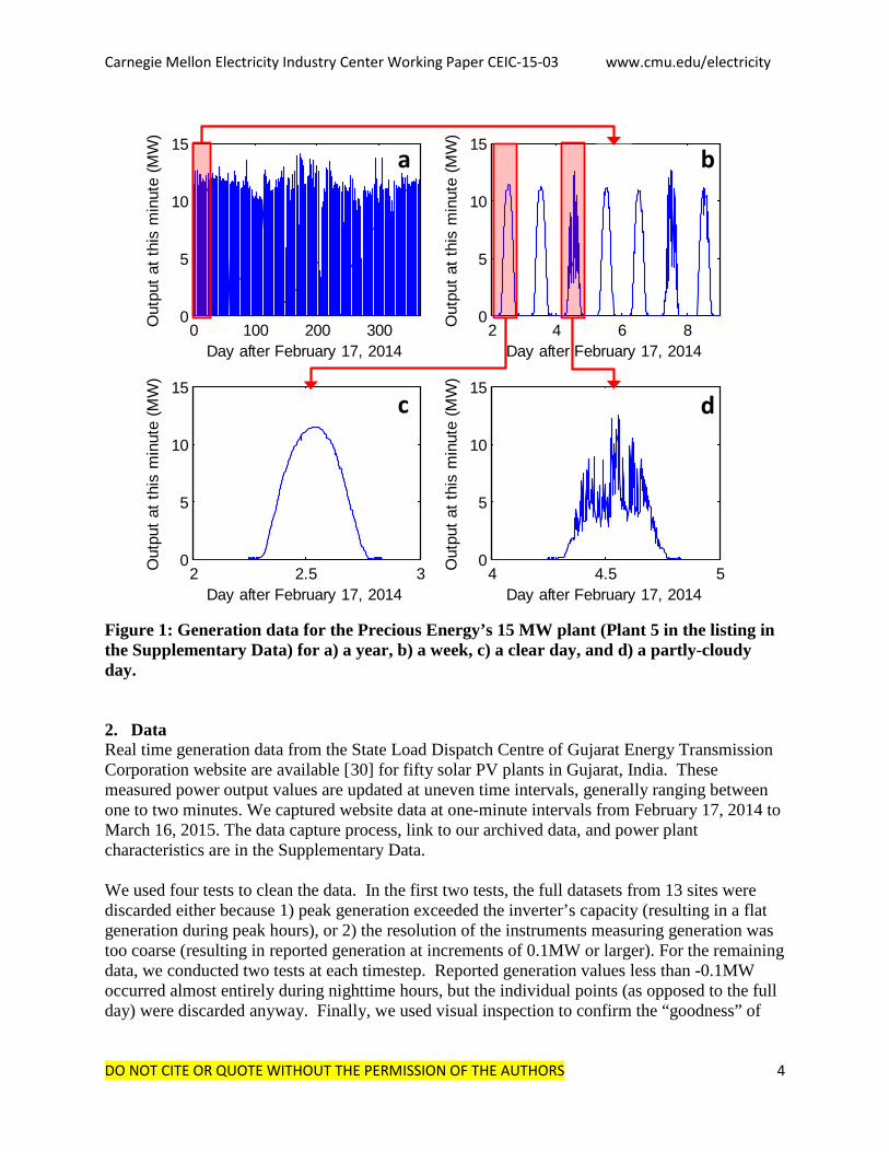
a. Calculating individual PSDs The Supplementary Data contains a PSD for each of the twenty plants. Most plants exhibit a spectrum at high frequencies ranging from f-1.23 to f-1.56, with the very large 322MW plant displaying a f-1.76 slope. We find that larger plant size is correlated with a steeper slope with a correlation coefficient of 0.57 at p<0.001 (Figure 3). These results agree with the approximately f-1.3 spectrum identified by previous research using generation data [1, 32, 33], (as well as the f-
0.7 spectrum identified when the y-axis is the square of the power [34]). This implies that there is still a large need for fast ramping power or demand response to compensate for PV fluctuations
Carnegie Mellon Electricity Industry Center Working Paper CEIC-15-03 www.cmu.edu/electricity
DO NOT CITE OR QUOTE WITHOUT THE PERMISSION OF THE AUTHORS 7
at high frequencies. Our results also validate for a real plant the conjecture based on irradiance data that as the capacity of the plant increases, it is likely that the plant will cover a larger horizontal area and thus be able to naturally filter out some of the variability [19, 20].
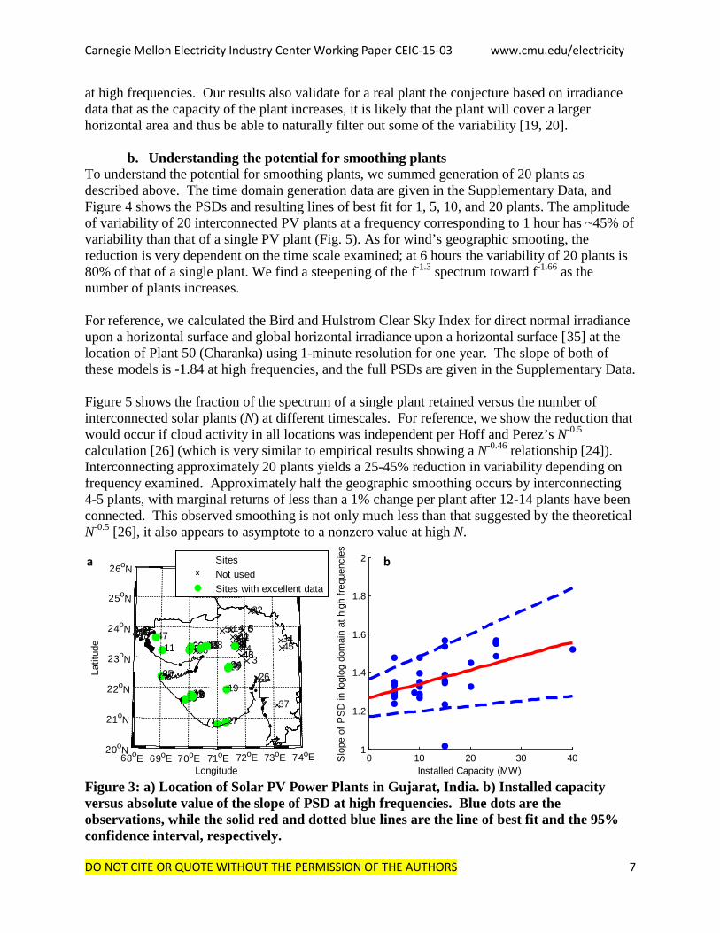
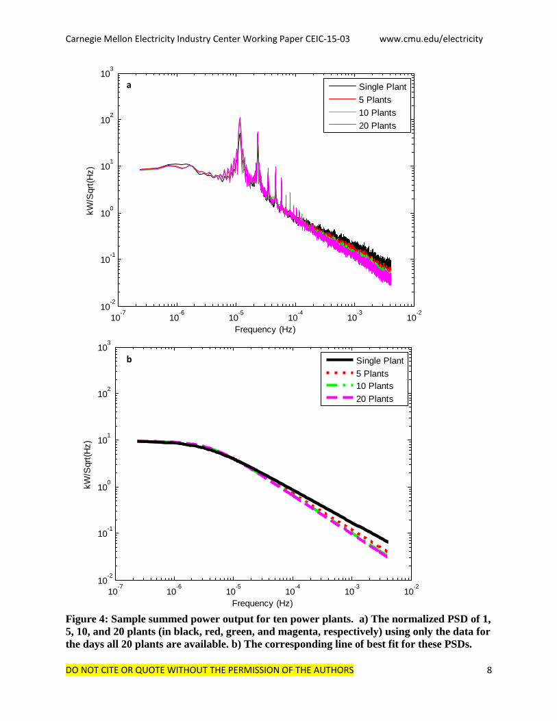
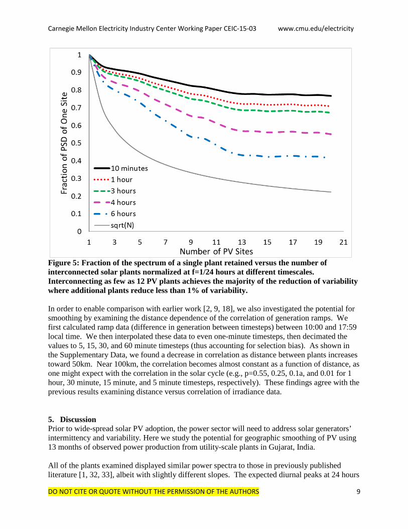
b. Understanding the potential for smoothing plants To understand the potential for smoothing plants, we summed generation of 20 plants as described above. The time domain generation data are given in the Supplementary Data, and Figure 4 shows the PSDs and resulting lines of best fit for 1, 5, 10, and 20 plants. The amplitude of variability of 20 interconnected PV plants at a frequency corresponding to 1 hour has ~45% of variability than that of a single PV plant (Fig. 5). As for wind’s geographic smooting, the reduction is very dependent on the time scale examined; at 6 hours the variability of 20 plants is 80% of that of a single plant. We find a steepening of the f-1.3 spectrum toward f-1.66 as the number of plants increases. For reference, we calculated the Bird and Hulstrom Clear Sky Index for direct normal irradiance upon a horizontal surface and global horizontal irradiance upon a horizontal surface [35] at the location of Plant 50 (Charanka) using 1-minute resolution for one year. The slope of both of these models is -1.84 at high frequencies, and the full PSDs are given in the Supplementary Data. Figure 5 shows the fraction of the spectrum of a single plant retained versus the number of interconnected solar plants (N) at different timescales. For reference, we show the reduction that would occur if cloud activity in all locations was independent per Hoff and Perez’s N-0.5 calculation [26] (which is very similar to empirical results showing a N-0.46 relationship [24]). Interconnecting approximately 20 plants yields a 25-45% reduction in variability depending on frequency examined. Approximately half the geographic smoothing occurs by interconnecting 4-5 plants, with marginal returns of less than a 1% change per plant after 12-14 plants have been connected. This observed smoothing is not only much less than that suggested by the theoretical N-0.5 [26], it also appears to asymptote to a nonzero value at high N.
Figure 3: a) Location of Solar PV Power Plants in Gujarat, India. b) Installed capacity versus absolute value of the slope of PSD at high frequencies. Blue dots are the observations, while the solid red and dotted blue lines are the line of best fit and the 95% confidence interval, respectively.
1 2
3
4 5 6
7 8 9
10
11 121314
15
16
171819
2021
22
23
24
25
26
27
28
29
30 31
32
3334
35
36
37
3839
40
4142
4344 4546
4748
49
50
68oE 69oE 70oE 71oE 72oE 73oE 74oE 20oN
21oN
22oN
23oN
24oN
25oN
26oN
Longitude
Latit
ude
SitesNot usedSites with excellent data
0 10 20 30 401
1.2
1.4
1.6
1.8
2
Installed Capacity (MW)
Slo
pe o
f PS
D in
logl
og d
omai
n at
hig
h fre
quen
cies
a b
Carnegie Mellon Electricity Industry Center Working Paper CEIC-15-03 www.cmu.edu/electricity
DO NOT CITE OR QUOTE WITHOUT THE PERMISSION OF THE AUTHORS 8
Figure 4: Sample summed power output for ten power plants. a) The normalized PSD of 1, 5, 10, and 20 plants (in black, red, green, and magenta, respectively) using only the data for the days all 20 plants are available. b) The corresponding line of best fit for these PSDs.
10-7
10-6
10-5
10-4
10-3
10-2
10-2
10-1
100
101
102
103
Frequency (Hz)
kW/S
qrt(H
z)
Single Plant5 Plants10 Plants20 Plants
10-7
10-6
10-5
10-4
10-3
10-2
10-2
10-1
100
101
102
103
Frequency (Hz)
kW/S
qrt(H
z)
Single Plant5 Plants10 Plants20 Plants
a
b
Carnegie Mellon Electricity Industry Center Working Paper CEIC-15-03 www.cmu.edu/electricity
DO NOT CITE OR QUOTE WITHOUT THE PERMISSION OF THE AUTHORS 9
Figure 5: Fraction of the spectrum of a single plant retained versus the number of interconnected solar plants normalized at f=1/24 hours at different timescales. Interconnecting as few as 12 PV plants achieves the majority of the reduction of variability where additional plants reduce less than 1% of variability. In order to enable comparison with earlier work [2, 9, 18], we also investigated the potential for smoothing by examining the distance dependence of the correlation of generation ramps. We first calculated ramp data (difference in generation between timesteps) between 10:00 and 17:59 local time. We then interpolated these data to even one-minute timesteps, then decimated the values to 5, 15, 30, and 60 minute timesteps (thus accounting for selection bias). As shown in the Supplementary Data, we found a decrease in correlation as distance between plants increases toward 50km. Near 100km, the correlation becomes almost constant as a function of distance, as one might expect with the correlation in the solar cycle (e.g., p=0.55, 0.25, 0.1a, and 0.01 for 1 hour, 30 minute, 15 minute, and 5 minute timesteps, respectively). These findings agree with the previous results examining distance versus correlation of irradiance data. 5. Discussion Prior to wide-spread solar PV adoption, the power sector will need to address solar generators’ intermittency and variability. Here we study the potential for geographic smoothing of PV using 13 months of observed power production from utility-scale plants in Gujarat, India. All of the plants examined displayed similar power spectra to those in previously published literature [1, 32, 33], albeit with slightly different slopes. The expected diurnal peaks at 24 hours
Carnegie Mellon Electricity Industry Center Working Paper CEIC-15-03 www.cmu.edu/electricity
DO NOT CITE OR QUOTE WITHOUT THE PERMISSION OF THE AUTHORS 10
and harmonics are present. At high frequencies, the plants exhibit a spectrum similar to cloud processes [36, 37]. These processes may be a function of the f-5/3 spectrum displayed by wind [32] and the f-1 spectrum displayed by hydrologic processes [38], or the PV plant may act as a low pass filter [34]. When interconnecting Gujarat PV plants, approximately half of the smoothing can be obtained through connecting 4-5 plants. Reduction in variability exhibits diminishing marginal returns, with interconnecting 12-14 plants yielding a f-1.66 spectrum. However, the largest plant, the 322MW Charanka Solar Park (at 23°54'N, 71°12'E), has an f-1.76 spectrum. This suggests that in Gujarat, the potential for smoothing may be limited to that obtained by one large plant. We further note that the PSD of the clear sky index at the Charanka Solar Park showed a f-1.84 slope, a steeper slope than all of our observed individual and combined plants. While this suggests more smoothing to reduce the noise from clouds may be possible, we are do not observe this smoothing, suggesting that other limiting factors may be in play. One possibility is that this study was limited to Gujarat, India, which according to the Koeppen classification system has a low-latitude (h), and either very dry (BW) or dry (BS) climate over the spatial area examined [39]. Gujarat may be a climatological region where generation at different plants cannot be considered independent, even across three degrees of longitude (almost 400 km); aggregating further plants outside this region may help filter out the noise of the clouds such that the slope will approach the clear sky model. Another possibility might occur because our plants are spread across several degrees of longitude with an approximately 7 minute difference in the solar peak across the data set. Consequently, while ramps in the clear sky index component are positively correlated at most times of the day, there would be some times where the ramps would be anti-correlated. This would suggest that geographic smoothing would be a function of longitude spanned (and thus distance between solar peaks), altering the theoretical limit. The power sector may also wish to compare the potential for geographic smoothing of solar PV to that from other renewable energy types. In comparison to the geographic smoothing of distributed wind plants in Texas [40], the PV plants we examined show substantially less smoothing. The two areas are of comparable size (roughly 400 km x 400km). Interconnecting 20 wind plants in Texas was found to reduce fluctuations at frequencies corresponding to 6 hours and 1 hour by 65% and 95% respectively, substantially more than the 23% and 45% observed for PV plants in Gujarat. We also find that when interconnecting observed PV plants, reaching marginal returns of less than a 1% change per plant requires two or three times the number of interconnected plants than for wind (12-14 for PV, 3-6 for wind). Since the area examined is comparable in size to many balancing areas, the relatively small amount of smoothing is likely to be relevant to practical application of solar photovoltaic generation at grid scale. Acknowledgements This research was supported by the Solar Energy Research Institute for India and the U.S. (SERIIUS) funded jointly by the U.S. Department of Energy subcontract DE AC36-08G028308 (Office of Science, Office of Basic Energy Sciences, and Energy Efficiency and Renewable Energy, Solar Energy Technology Program, with support from the Office of International

Carnegie Mellon Electricity Industry Center Working Paper CEIC-15-03 www.cmu.edu/electricity
DO NOT CITE OR QUOTE WITHOUT THE PERMISSION OF THE AUTHORS 11
Affairs) and the Government of India subcontract IUSSTF/JCERDC-SERIIUS/2012 dated 22nd Nov. 2012.
Carnegie Mellon Electricity Industry Center Working Paper CEIC-15-03 www.cmu.edu/electricity
DO NOT CITE OR QUOTE WITHOUT THE PERMISSION OF THE AUTHORS 12
References 1 Curtright, A.E.; Apt, J. (2008). The character of power output from utility-scale photovoltaic systems. Progress in Photovoltaics: Research and Applications. 16(3), 241–247. 2 Mills, A.D.; Wiser, R.H. (2010). Implications of Wide-Area Geographic Diversity for Short- Term Variability of Solar Power. Technical Report LBNL-3884E. 3 Edenhofer, O.; Pichs-Madruga, R.; Sokona, Y.; Seyboth, K.; Matschoss, P.; Kadner, S.; Zwickel, T.; Eickemeier, P.; Hansen, G.; Schlömer, S.; von Stechow, C. (Eds.). IPCC special report on renewable energy sources and climate change mitigation. Prepared by Working Group III of the intergovernmental panel on climate change, Cambridge University Press, United Kingdom and New York, NY, USA (2011), p. 1075 4 Widén, J.; Carpman, N.; Castellucci, V.; Lingfors, D.; Olauson, J.; Remouit, F.; Bergkvist, M.; Grabbe, M.; Waters, R. (2015). Variability assessment and forecasting of renewables: A review for solar, wind, wave and tidal resources. Renewable and Sustainable Energy Reviews. 44(1), 356-375. 5 McConnell, B.W.; Hadley, S.W.; Xu, Y. (2011). A Review of Barriers to and Opportunities for the Integration of Renewable Energy. ORNL/TM/-2010/138 . 6 Denholm, P.; Margolis, R.M.; (2007) Evaluating the limits of solar photovoltaics (PV) in electric power systems utilizing energy storage and other enabling technologies. Energy Policy. 35(1), 4424–4433. 7 Kleissel, Jan (2013). Solar Energy Forecasting and Resource Assessment. Academic Press: Amsterdam. 8 Long, C.N.; Ackerman, T.P. (1995). Surface Measurements of Solar Irradiance: A Study of the Spatial Correlation between Simultaneous Measurements at Separated Sites. Journal of Applied Meteorology. 34(1), 1039–1046. 9 Barnett, T.P.; Ritchie, J.; Foat, J.; Stokes, G. (1998). On the Space–Time Scales of the Surface Solar Radiation Field. Journal of Climate. 11(1), 88–96. 10 Lave, M.; Kleissl, J. (2010). Solar variability of four sites across the state of Colorado. Renewable Energy. 35(12), 2867–2873. 11 Hinkleman, L. (2013). Differences between along-wind and cross-wind solar irradiance variability on small spatial scales. Solar Energy. 88(1), 192–203. 12 Otani, K.; Minowa, J.; Kurokawa, K. (1997). Study on area solar irradiance for analyzing areally‐totalized PV systems. Solar Energy Materials and Solar Cells. 47(1), 281‐288. 13 Lave, M.; Kleissl, J.; Arias-Castro, E. (2012). High-frequency irradiance fluctuations and geographic smoothing. Solar Energy. 86(8), 2190–2199. 14 Kawaski, N.; Oozeki, T.; Otani, K.; Kurokawa, K. (2006). An evaluation method of the fluctuation characteristics of photovoltaic systems by using frequency analysis. Solar Energy Materials and Solar Cells. 90(18-19), 3356-3363. 15 Jewell, W.T., Unruh, T.D., 1990. Limits on cloud-induced fluctuation in photovoltaic generation. IEEE Transactions on Energy Conversion. 5(1), 8–14. 16 Kern, E.J.; Russell, M. (1988). Spatial and temporal irradiance variations over large array fields. Photovoltaic Specialists Conference, Conference Record of the Twentieth IEEE. 2(1), 1043-1050. 17 Wiemken, E.; Beyer, H.G.; Heydenreich, W.; Kiefer, K. (2001). Power characteristics of PV ensembles: experiences from the combined power production of 100 grid connected PV systems distributed over the area of Germany. Solar Energy. 70(6), 513–518.
Carnegie Mellon Electricity Industry Center Working Paper CEIC-15-03 www.cmu.edu/electricity
DO NOT CITE OR QUOTE WITHOUT THE PERMISSION OF THE AUTHORS 13
18 Rowlands, I.H.; Kemery, B.P.; Beausoleil-Morrison, I. (2014). Managing solar-PV variability with geographical dispersion: An Ontario (Canada) case-study. Renewable Energy. 68(1), 171–180. 19 Kankiewicz A, Moon D, Sengupta M. Observed impacts of transient clouds on utility-scale PV fields. ASES National Solar Conference. Phoenix, AZ, USA; 2010. 20 Marcos, J.; Marroyo, L.; Lorenzo, E.; Alvira, D.; Izco, E. (2011) Power Output Fluctuations in Large Scale Pv Plants: One Year Observations with One Second Resolution and a Derived Analytic Model. Progress in Photovoltaics: Research and Applications. 19, 218–227. 21 Golnas A, Bryan JM. Output variability in Europe׳s largest PV power plant. In: Proceedings of the 26th European photovoltaic solar energy conference and exhibition; 2011. 22 Golnas A, Voss S. (2010). Power output variability of PV system fleets in three utility service territories in New Jersey and California. In: Proceedings of the 2010 35th IEEE photovoltaic specialists conference (PVSC). pp. 535–539. 23 Golnas A, Bryan JM. (2011). 11-Month power output variability study of a PV system fleet in New Jersey. In: Proceedings of the 26th European photovoltaic solar energy conference and exhibition. 24 Marcos, J.; Marroyo, L.; Lorenzo, E.; García, M. (2012) Smoothing of PV Power Fluctuations by Geographical Dispersion. Progress in Photovoltaics: Research and Applications. 20(2), 226–37. 25 Van Haaren, R.; Morjaria, M.; Fthenakis, V. (2014). Empirical Assessment of Short-Term Variability from Utility-Scale Solar PV Plants. Progress in Photovoltaics: Research and Applications 22(5), 548–59. 26 Hoff, T. E.; Perez, R. (2012). Modeling PV Fleet Output Variability. Solar Energy. 86(8): 2177–89. 27 Murata, A.; Yamaguchi, H.; Otani, K. (2009). A method of estimating the output fluctuation of many photovoltaic power generation systems dispersed in a wide area. Electrical Engineering in Japan. 166(4), 9-19. 28 Cha, P.; Molinder,J. (2006). Fundamentals of Signals and Systems: A Building Block Approach. Cambridge Press: New York. 29 Press, W.H.; Teukolsky, S.A.; Vetterling, W.T.; Flannery, B.P. (1992). Numerical Recipes in FORTRAN: The Art of Scientific Computing. Second ed. Cambridge University Press, Cambridge. 30 SLDC-Gujarat. “State Load Despatch Centre (SLDC) – Real-Time System Data”. https://www.sldcguj.com/RealTimeData/GujSolar.asp Accessed by authors every minute from February 17, 2014 to March 16, 2015. 31 Lomb, N.R. (1976). Least-squares frequency analysis of unevenly spaced data. Astrophysics and Space Science. 39, 447–462. 32 Apt, J.; Jaramillo, P. Variable Renewable Energy and the Electricity Grid. RFF Press: Oxford, 2014. 33 Lueken, C.; Cohen, G.E.; Apt, J. (2012). Costs of solar and wind power variability for reducing CO2 emissions. Environmental Science & Technology. 46(1), 9761-9767. 34 Marcos, J.; Marroyo, L.; Lorenzo, E.; Alvira, E.; Izco, E. (2011). From Irradiance to Output Power Fluctuations: The PV Plant as a Low Pass Filter. Progress in Photovoltaics: Research and Applications. 19(5), 505–10.

Carnegie Mellon Electricity Industry Center Working Paper CEIC-15-03 www.cmu.edu/electricity
DO NOT CITE OR QUOTE WITHOUT THE PERMISSION OF THE AUTHORS 14
35 Bird, R.E.; Hulstrom, R.L. (1991). A Simplified Clear Sky Model for Direct and Diffuse Insolation on Horizontal Surfaces. SERI Technical Report SERI/TR-642-761. Solar Energy Research Institute, Golden, CO. 36 Fliflet, A.W.; Manheimer, W.M. (2006). Measurement of Correlation Functions and Power Spectra in Clouds Using the NRL WARLOC Radar. IEEE Transactions on Geosciences and Remote Sensing. 44(11), p. 3247. 37 von Savigny, C.; Davis, A.B.; Funk,O.; Pfeilsticker, K. (2002). Time-series of zenith radiance and surface flux under cloudy skies: Radiative smoothing, optical thickness retrievals and large-scale stationarity. Geophysical Research Letters. 29(17), p. 1825. 38 Kirchner, J.W.; Neal, C (2013). Universal fractal scaling in stream chemistry and its implications for solute transport and water quality trend detection. PNAS. 110(30), 12213-12218. 39 Peel, M.C.; Finlayson, B.L.; McMahon, T. A. (2007). Updated world map of the Köppen–Geiger climate classification. Hydrology and Earth System Sciences. 11, 1633–1644. 40 Katzenstein, W.; Fertig, E.; Apt, J. (2010). The variability of interconnected wind plants. Energy Policy. 38(1), 4400–4410.
Carnegie Mellon Electricity Industry Center Working Paper CEIC-15-03 www.cmu.edu/electricity
DO NOT CITE OR QUOTE WITHOUT THE PERMISSION OF THE AUTHORS S 1
Geographic smoothing of solar PV: Results from Gujarat Supplementary Data Kelly Klima†,* Jay Apt†, ‡ July 27, 2015 †Department of Engineering and Public Policy, Carnegie Mellon University, 5000 Forbes Avenue, Pittsburgh, PA 15213, USA ‡Tepper School of Business, Carnegie Mellon University, 5000 Forbes Avenue, Pittsburgh, PA 15213, USA * Corresponding Author: [email protected]; 412-268-3705 Table of Contents: 1. URL for the archived data used in this research .................................................................................... S 2
2. Location and size of the plants used ...................................................................................................... S 3
3. Power spectral densities calculated using the Lomb periodiogram with a line of best fit via Eq. 1 for all plants with good data ................................................................................................................................ S 5
4. Power spectral densities calculated using the Lomb periodiogram for Clear Sky Index ..................... S 42
5. Time series data of summed generation ............................................................................................. S 45
6. Scatterplot of distance versus correlation for the Gujarat plant generations ..................................... S 46

Carnegie Mellon Electricity Industry Center Working Paper CEIC-15-03 www.cmu.edu/electricity
DO NOT CITE OR QUOTE WITHOUT THE PERMISSION OF THE AUTHORS S 2
1. URL for the archived data used in this research Real time generation data from the State Load Dispatch Centre of Gujarat Energy Transmission Corporation website are available for 50 solar PV plants in Gujarat, India. The website is: https://www.sldcguj.com/RealTimeData/GujSolar.asp These values are updated at uneven time intervals, generally ranging between one to two minutes. Since the State Load Dispatch Centre does not archive the data, we captured website data at one-minute intervals from February 17, 2014 to March 16, 2015. We have made these data available at: http://wpweb2.tepper.cmu.edu/electricity/datadownloads.asp . We used four tests to clean the data. In the first two tests, the full datasets from 13 sites were discarded either because 1) peak generation greatly exceeded the inverter (resulting in a flat generation during peak hours), or 2) the resolution of the instruments measuring generation was too coarse (resulting in reported generation at increments of 0.1MW or larger). For the remaining data, we conducted two tests at each timestep. Reported generation values less than -0.1MW occurred almost entirely during nighttime hours, but the individual points (as opposed to the full day) were discarded anyway. Finally, we used visual inspection was used to confirm the “goodness” of the data, resulting in discarding one additional day of a small MW plant that our data cleansing algorithm had not captured.
Carnegie Mellon Electricity Industry Center Working Paper CEIC-15-03 www.cmu.edu/electricity
DO NOT CITE OR QUOTE WITHOUT THE PERMISSION OF THE AUTHORS S 3
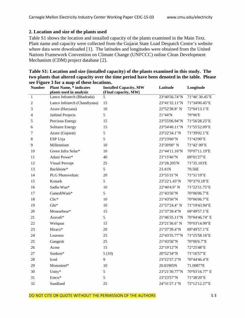
2. Location and size of the plants used Table S1 shows the location and installed capacity of the plants examined in the Main Text. Plant name and capacity were collected from the Gujarat State Load Despatch Centre’s website where data were downloaded [1]. The latitudes and longitudes were obtained from the United Nations Framework Convention on Climate Change (UNFCCC) online Clean Development Mechanism (CDM) project database [2]. Table S1: Location and size (installed capacity) of the plants examined in this study. The two plants that altered capacity over the time period have been denoted in the table. Please see Figure 3 for a map of these locations. Number Plant Name, * indicates
plants used in analysis Installed Capacity, MW (Final capacity, MW)
Latitude Longitude
1 Lanco Infratech (Bhadrada) 5 23°40'56.74"N 71°46' 30.45"E 2 Lanco Infratech (Chandiyana) 15 23°41'32.11"N 71°34'00.45"E 3 Azure (Haryana) 10 22°52'38.8" N 72°04'13.1"E 4 Jaihind Projects 5 21°44′N 70°06′E 5 Precious Energy 15 23°55'06.94"N 71°56'28.25"E 6 Solitaire Energy 15 23°54'40.11"N 71°55'52.09"E 7 Azure (Gujarat) 5 23°22'34.1"N 71°39'02.1"E 8 ESP Urja 5 23°23'60"N 71°42'00"E 9 Millennium 10 23°30'00" N 71°42' 00"E 10 Green Infra Solar* 10 21°44'11.16''N 70°07'11.19''E 11 Adani Power* 40 23°15'46″N 69°01'27"E 12 Visual Percept 25 23°28.205'N 71°35.103'E 13 Backbone* 5 23.41N 70.56E 14 PLG Photovoltaic 20 23°55'31"N 71°31'19"E 15 Konark 5 23°22'1.43"N 70°37'0.18"E 16 Sadla-Waa* 10 22°40'4.9" N 71°22'51.75"E 17 GaneshWani* 5 21°43'56"N 70°06'06.7"E 18 Cbc* 10 21°43'56"N 70°06'06.7"E 19 Ghi* 10 21°57'24.4" N 71°19'43.94"E 20 Mosearbear* 15 21°37'39.4"N 69°49'57.1"E 21 Aravali* 5 21°46'35.11"N 70°04'46.74" E 22 Welspun 15 23°21'36.6" N 70°03'14.99"E 23 Hiraco* 20 21°37'39.4"N 69°49'57.1"E 24 Louroux 25 22°43'35.77"N 71°25'58.16"E 25 Gangesh 25 21°43'56"N 70°06'6.7"E 26 Acme 15 22°19'12"N 72°25'48"E 27 Sunkon* 5 (10) 20°52'34"N 71°16'57"E 28 Icml 9 23°22'37.2"N 70°44'46.4"E 29 Monosteel* 10 20.81905N 71.00877E 30 Unity* 5 23°21'30.77"N 70°03'16.77" E 31 Emco* 5 23°23'57"N 71°38'20"E 32 Sandland 25 24°31'27.1"N 72°12'12.27"E
Carnegie Mellon Electricity Industry Center Working Paper CEIC-15-03 www.cmu.edu/electricity
DO NOT CITE OR QUOTE WITHOUT THE PERMISSION OF THE AUTHORS S 4
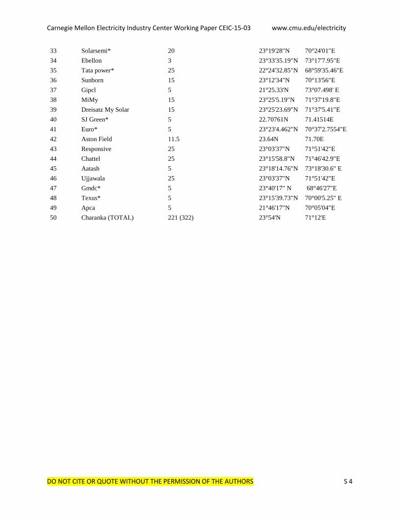
33 Solarsemi* 20 23°19'28"N 70°24'01"E 34 Ebellon 3 23°33'35.19"N 73°17'7.95"E 35 Tata power* 25 22°24'32.85"N 68°59'35.46"E 36 Sunborn 15 23°12'34"N 70°13'56"E 37 Gipcl 5 21°25.33'N 73°07.498' E 38 MiMy 15 23°25'5.19"N 71°37'19.8"E 39 Dreisatz My Solar 15 23°25'23.69"N 71°37'5.41"E 40 SJ Green* 5 22.70761N 71.41514E 41 Euro* 5 23°23'4.462"N 70°37'2.7554"E 42 Aston Field 11.5 23.64N 71.70E 43 Responsive 25 23°03'37"N 71°51'42"E 44 Chattel 25 23°15'58.8"N 71°46'42.9"E 45 Aatash 5 23°18'14.76"N 73°18'30.6" E 46 Ujjawala 25 23°03'37"N 71°51'42"E 47 Gmdc* 5 23°40'17" N 68°46'27"E 48 Texus* 5 23°15'39.73"N 70°00'5.25" E 49 Apca 5 21°46'17"N 70°05'04"E 50 Charanka (TOTAL) 221 (322) 23°54'N 71°12'E

Carnegie Mellon Electricity Industry Center Working Paper CEIC-15-03 www.cmu.edu/electricity
DO NOT CITE OR QUOTE WITHOUT THE PERMISSION OF THE AUTHORS S 5
3. Power spectral densities calculated using the Lomb periodiogram with a line of best fit via Eq. 1 for all plants with good data This section contains the power spectral densities (PSDs) for 36 plants with sufficient good data (Figures S1-S36). We calculated using PSDs the Lomb periodiogram and displayed the line of best fit via Eq. 1. At high frequency we observed two types of PSD characteristics. The first characteristic exhibited a constant spectrum of approximately f-1.3 at all frequencies greater than 12 hours, which agrees with the spectrum identified by previous research [3, 4, 5]. The second exhibited a spectrum of approximately f -1.3 between 3 to 12 hours. At above a “corner frequency” of approximately 10-3 Hz, these plants exhibited approximately an f -3 spectrum. While this behavior was not directly noted in the text of previous studies, the existence of a corner frequency agrees well with the figures of PSDs as found by previous research [3, 4, 5]. The existence of this corner frequency does not appear to be correlated to the location, generation, or fraction of data points retained. We hypothesize the corner frequency may have something to do with different physical arrangements of the plant (presence of inverter, angle, ground cover ratio, tracking or not, thin film or not) and/or cloud characteristics, but were unable to test for these potential relationships. Marcos et al suggest this is the power plant acting as a low pass filter [6]. Since we could not conclude what might be causing the corner frequency and therefore if the data were corrupted or not, we conducted the remainder of the results as discussed in the main text for twenty locations displaying a constant spectrum of approximately f-1.3 at all frequencies greater than 12 hours.
Carnegie Mellon Electricity Industry Center Working Paper CEIC-15-03 www.cmu.edu/electricity
DO NOT CITE OR QUOTE WITHOUT THE PERMISSION OF THE AUTHORS S 6
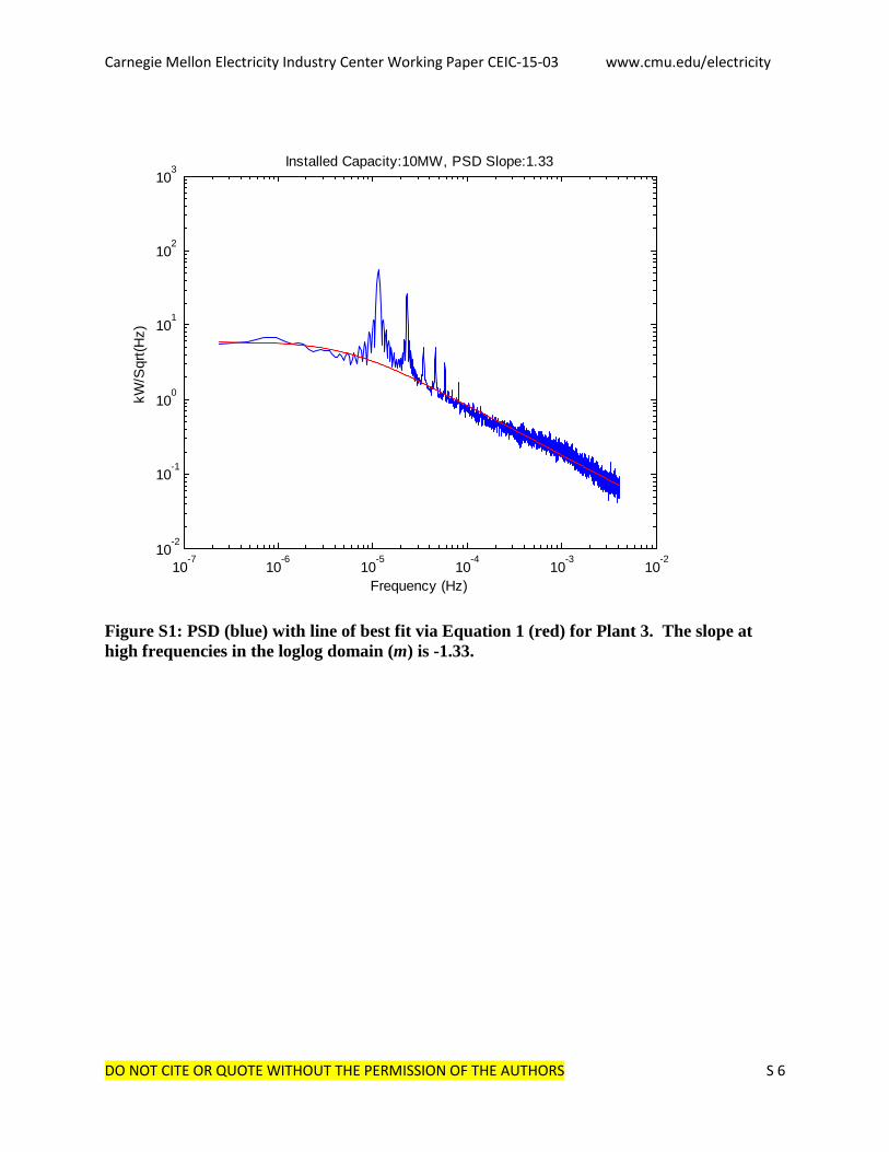
Figure S1: PSD (blue) with line of best fit via Equation 1 (red) for Plant 3. The slope at high frequencies in the loglog domain (m) is -1.33.
10-7
10-6
10-5
10-4
10-3
10-2
10-2
10-1
100
101
102
103
Frequency (Hz)
kW/S
qrt(H
z)Installed Capacity:10MW, PSD Slope:1.33
Carnegie Mellon Electricity Industry Center Working Paper CEIC-15-03 www.cmu.edu/electricity
DO NOT CITE OR QUOTE WITHOUT THE PERMISSION OF THE AUTHORS S 7
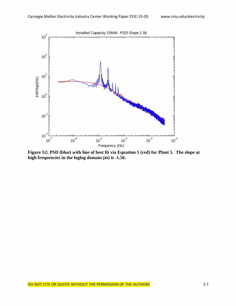
Figure S2: PSD (blue) with line of best fit via Equation 1 (red) for Plant 5. The slope at high frequencies in the loglog domain (m) is -1.56.
10-7
10-6
10-5
10-4
10-3
10-2
10-2
10-1
100
101
102
103
Frequency (Hz)
kW/S
qrt(H
z)Installed Capacity:15MW, PSD Slope:1.56

Carnegie Mellon Electricity Industry Center Working Paper CEIC-15-03 www.cmu.edu/electricity
DO NOT CITE OR QUOTE WITHOUT THE PERMISSION OF THE AUTHORS S 8
Figure S3: PSD (blue) with line of best fit via Equation 1 (red) for Plant 6. The slope at high frequencies in the loglog domain (m) is -1.51.
10-7
10-6
10-5
10-4
10-3
10-2
10-2
10-1
100
101
102
103
Frequency (Hz)
kW/S
qrt(H
z)Installed Capacity:15MW, PSD Slope:1.51

Carnegie Mellon Electricity Industry Center Working Paper CEIC-15-03 www.cmu.edu/electricity
DO NOT CITE OR QUOTE WITHOUT THE PERMISSION OF THE AUTHORS S 9
Figure S4: PSD (blue) with line of best fit via Equation 1 (red) for Plant 7. The slope at high frequencies in the loglog domain (m) is -1.34.
10-7
10-6
10-5
10-4
10-3
10-2
10-2
10-1
100
101
102
103
Frequency (Hz)
kW/S
qrt(H
z)Installed Capacity:5MW, PSD Slope:1.34

Carnegie Mellon Electricity Industry Center Working Paper CEIC-15-03 www.cmu.edu/electricity
DO NOT CITE OR QUOTE WITHOUT THE PERMISSION OF THE AUTHORS S 10
Figure S5: PSD (blue) with line of best fit via Equation 1 (red) for Plant 8. The slope at high frequencies in the loglog domain (m) is -1.3.
10-7
10-6
10-5
10-4
10-3
10-2
10-2
10-1
100
101
102
103
Frequency (Hz)
kW/S
qrt(H
z)Installed Capacity:5MW, PSD Slope:1.3

Carnegie Mellon Electricity Industry Center Working Paper CEIC-15-03 www.cmu.edu/electricity
DO NOT CITE OR QUOTE WITHOUT THE PERMISSION OF THE AUTHORS S 11
Figure S6: PSD (blue) with line of best fit via Equation 1 (red) for Plant 10. The slope at high frequencies in the loglog domain (m) is -1.39.
10-7
10-6
10-5
10-4
10-3
10-2
10-2
10-1
100
101
102
103
Frequency (Hz)
kW/S
qrt(H
z)Installed Capacity:10MW, PSD Slope:1.39
Carnegie Mellon Electricity Industry Center Working Paper CEIC-15-03 www.cmu.edu/electricity
DO NOT CITE OR QUOTE WITHOUT THE PERMISSION OF THE AUTHORS S 12
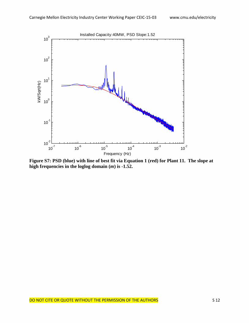
Figure S7: PSD (blue) with line of best fit via Equation 1 (red) for Plant 11. The slope at high frequencies in the loglog domain (m) is -1.52.
10-7
10-6
10-5
10-4
10-3
10-2
10-2
10-1
100
101
102
103
Frequency (Hz)
kW/S
qrt(H
z)Installed Capacity:40MW, PSD Slope:1.52

Carnegie Mellon Electricity Industry Center Working Paper CEIC-15-03 www.cmu.edu/electricity
DO NOT CITE OR QUOTE WITHOUT THE PERMISSION OF THE AUTHORS S 13
Figure S8: PSD (blue) with line of best fit via Equation 1 (red) for Plant 13. The slope at high frequencies in the loglog domain (m) is -1.29.
10-7
10-6
10-5
10-4
10-3
10-2
10-2
10-1
100
101
102
103
Frequency (Hz)
kW/S
qrt(H
z)Installed Capacity:5MW, PSD Slope:1.29

Carnegie Mellon Electricity Industry Center Working Paper CEIC-15-03 www.cmu.edu/electricity
DO NOT CITE OR QUOTE WITHOUT THE PERMISSION OF THE AUTHORS S 14
Figure S9: PSD (blue) with line of best fit via Equation 1 (red) for Plant 16. The slope at high frequencies in the loglog domain (m) is -1.29.
10-7
10-6
10-5
10-4
10-3
10-2
10-2
10-1
100
101
102
103
Frequency (Hz)
kW/S
qrt(H
z)Installed Capacity:10MW, PSD Slope:1.29

Carnegie Mellon Electricity Industry Center Working Paper CEIC-15-03 www.cmu.edu/electricity
DO NOT CITE OR QUOTE WITHOUT THE PERMISSION OF THE AUTHORS S 15
Figure S10: PSD (blue) with line of best fit via Equation 1 (red) for Plant 17. The slope at high frequencies in the loglog domain (m) is -1.36.
10-7
10-6
10-5
10-4
10-3
10-2
10-2
10-1
100
101
102
103
Frequency (Hz)
kW/S
qrt(H
z)Installed Capacity:5MW, PSD Slope:1.36
Carnegie Mellon Electricity Industry Center Working Paper CEIC-15-03 www.cmu.edu/electricity
DO NOT CITE OR QUOTE WITHOUT THE PERMISSION OF THE AUTHORS S 16
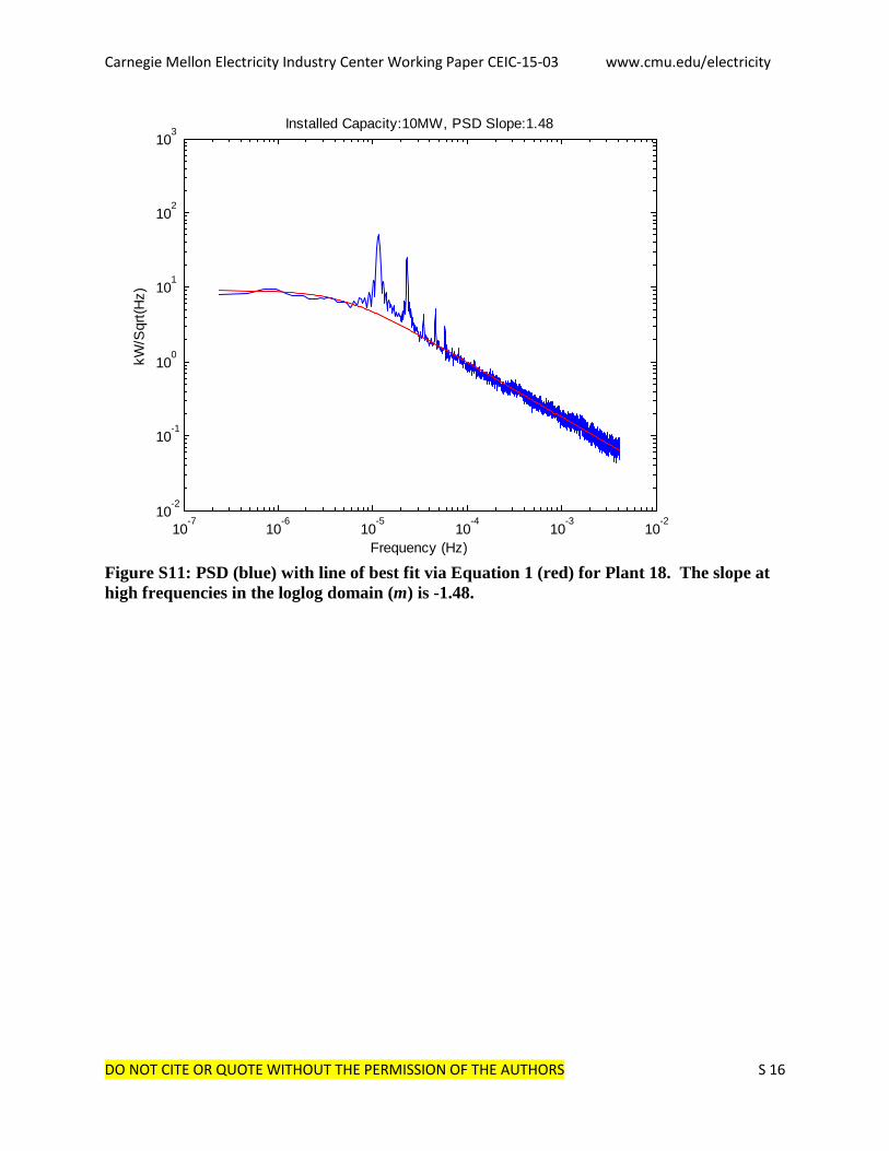
Figure S11: PSD (blue) with line of best fit via Equation 1 (red) for Plant 18. The slope at high frequencies in the loglog domain (m) is -1.48.
10-7
10-6
10-5
10-4
10-3
10-2
10-2
10-1
100
101
102
103
Frequency (Hz)
kW/S
qrt(H
z)Installed Capacity:10MW, PSD Slope:1.48
Carnegie Mellon Electricity Industry Center Working Paper CEIC-15-03 www.cmu.edu/electricity
DO NOT CITE OR QUOTE WITHOUT THE PERMISSION OF THE AUTHORS S 17
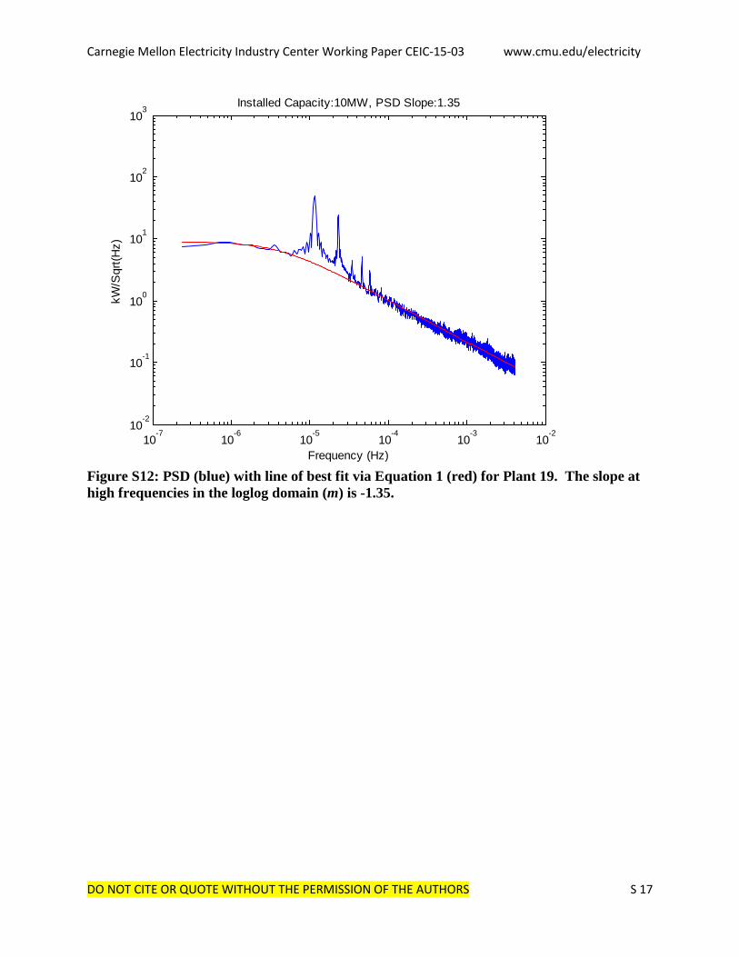
Figure S12: PSD (blue) with line of best fit via Equation 1 (red) for Plant 19. The slope at high frequencies in the loglog domain (m) is -1.35.
10-7
10-6
10-5
10-4
10-3
10-2
10-2
10-1
100
101
102
103
Frequency (Hz)
kW/S
qrt(H
z)Installed Capacity:10MW, PSD Slope:1.35
Carnegie Mellon Electricity Industry Center Working Paper CEIC-15-03 www.cmu.edu/electricity
DO NOT CITE OR QUOTE WITHOUT THE PERMISSION OF THE AUTHORS S 18
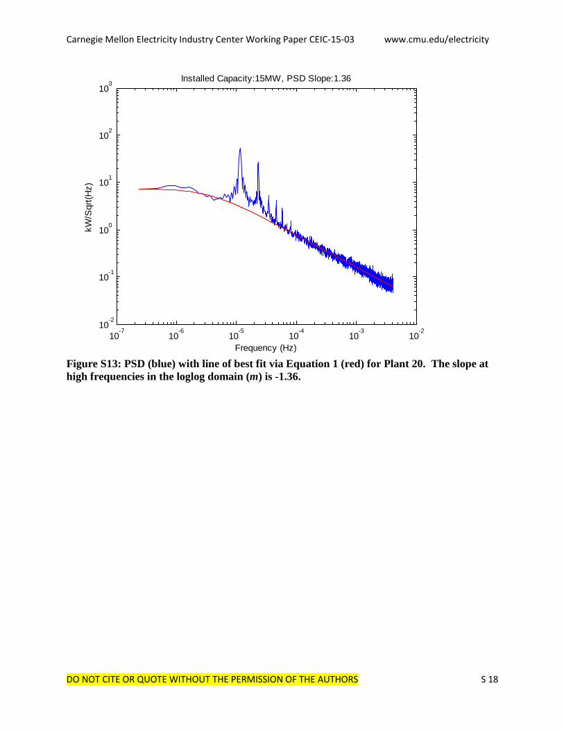
Figure S13: PSD (blue) with line of best fit via Equation 1 (red) for Plant 20. The slope at high frequencies in the loglog domain (m) is -1.36.
10-7
10-6
10-5
10-4
10-3
10-2
10-2
10-1
100
101
102
103
Frequency (Hz)
kW/S
qrt(H
z)Installed Capacity:15MW, PSD Slope:1.36
Carnegie Mellon Electricity Industry Center Working Paper CEIC-15-03 www.cmu.edu/electricity
DO NOT CITE OR QUOTE WITHOUT THE PERMISSION OF THE AUTHORS S 19
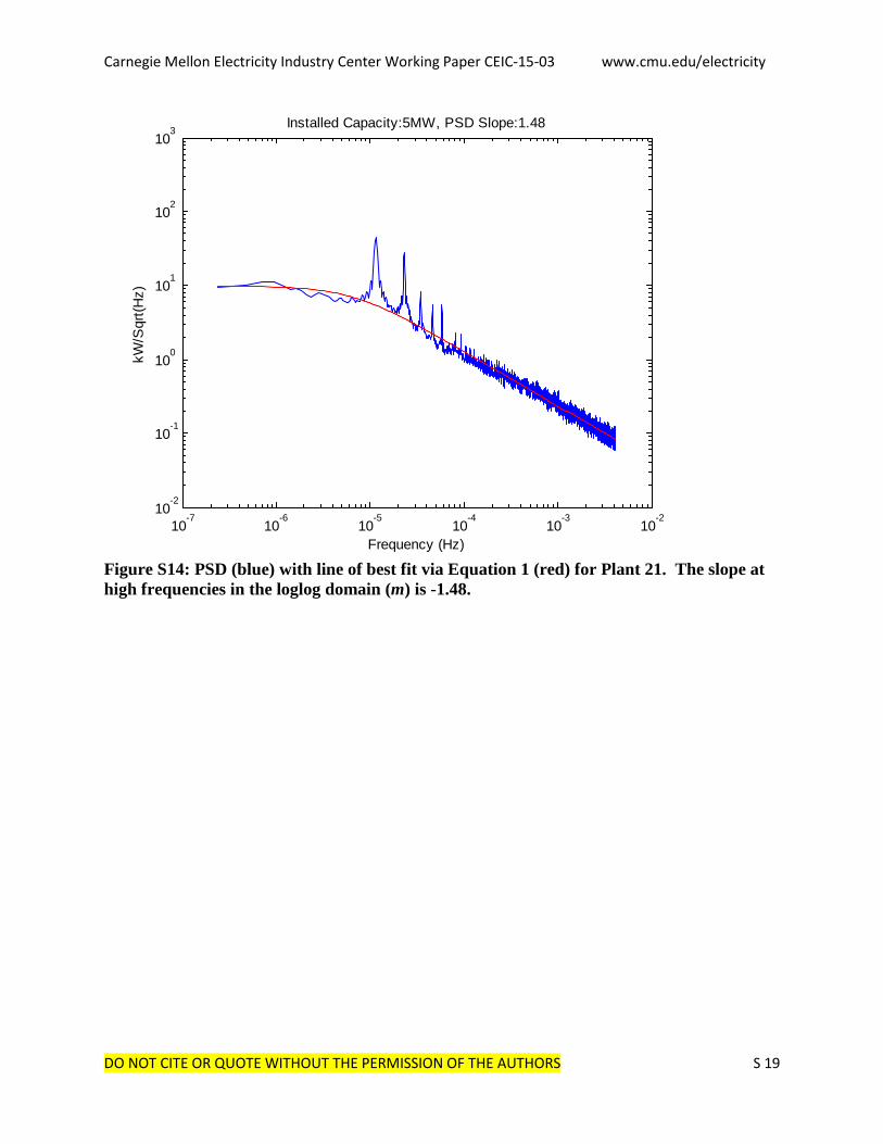
Figure S14: PSD (blue) with line of best fit via Equation 1 (red) for Plant 21. The slope at high frequencies in the loglog domain (m) is -1.48.
10-7
10-6
10-5
10-4
10-3
10-2
10-2
10-1
100
101
102
103
Frequency (Hz)
kW/S
qrt(H
z)Installed Capacity:5MW, PSD Slope:1.48
Carnegie Mellon Electricity Industry Center Working Paper CEIC-15-03 www.cmu.edu/electricity
DO NOT CITE OR QUOTE WITHOUT THE PERMISSION OF THE AUTHORS S 20
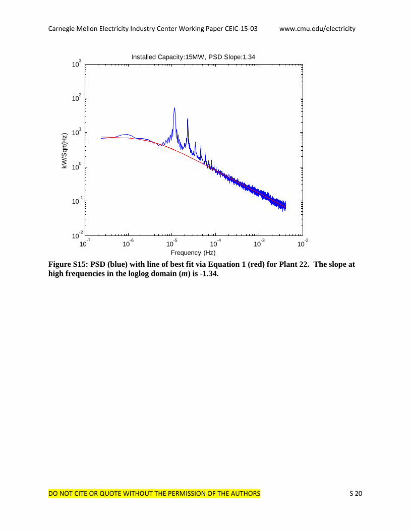
Figure S15: PSD (blue) with line of best fit via Equation 1 (red) for Plant 22. The slope at high frequencies in the loglog domain (m) is -1.34.
10-7
10-6
10-5
10-4
10-3
10-2
10-2
10-1
100
101
102
103
Frequency (Hz)
kW/S
qrt(H
z)Installed Capacity:15MW, PSD Slope:1.34

Carnegie Mellon Electricity Industry Center Working Paper CEIC-15-03 www.cmu.edu/electricity
DO NOT CITE OR QUOTE WITHOUT THE PERMISSION OF THE AUTHORS S 21
Figure S16: PSD (blue) with line of best fit via Equation 1 (red) for Plant 23. The slope at high frequencies in the loglog domain (m) is -1.33.
10-7
10-6
10-5
10-4
10-3
10-2
10-2
10-1
100
101
102
103
Frequency (Hz)
kW/S
qrt(H
z)Installed Capacity:20MW, PSD Slope:1.33

Carnegie Mellon Electricity Industry Center Working Paper CEIC-15-03 www.cmu.edu/electricity
DO NOT CITE OR QUOTE WITHOUT THE PERMISSION OF THE AUTHORS S 22
Figure S17: PSD (blue) with line of best fit via Equation 1 (red) for Plant 24. The slope at high frequencies in the loglog domain (m) is -1.49.
10-7
10-6
10-5
10-4
10-3
10-2
10-2
10-1
100
101
102
103
Frequency (Hz)
kW/S
qrt(H
z)Installed Capacity:25MW, PSD Slope:1.49
Carnegie Mellon Electricity Industry Center Working Paper CEIC-15-03 www.cmu.edu/electricity
DO NOT CITE OR QUOTE WITHOUT THE PERMISSION OF THE AUTHORS S 23
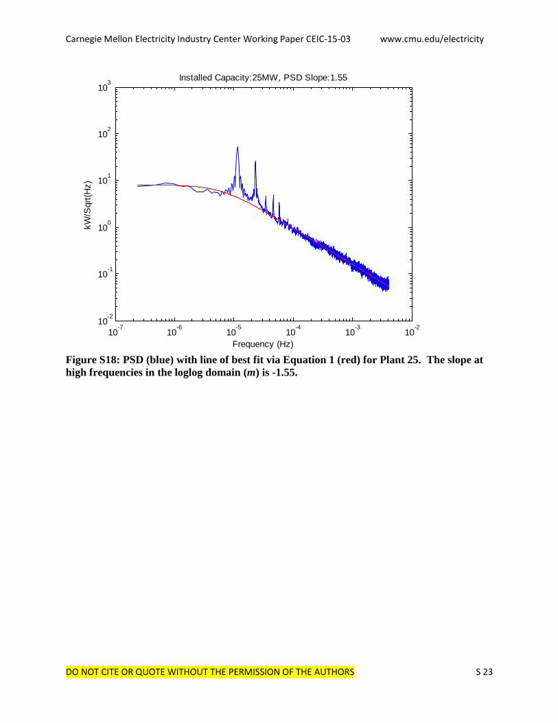
Figure S18: PSD (blue) with line of best fit via Equation 1 (red) for Plant 25. The slope at high frequencies in the loglog domain (m) is -1.55.
10-7
10-6
10-5
10-4
10-3
10-2
10-2
10-1
100
101
102
103
Frequency (Hz)
kW/S
qrt(H
z)Installed Capacity:25MW, PSD Slope:1.55
Carnegie Mellon Electricity Industry Center Working Paper CEIC-15-03 www.cmu.edu/electricity
DO NOT CITE OR QUOTE WITHOUT THE PERMISSION OF THE AUTHORS S 24
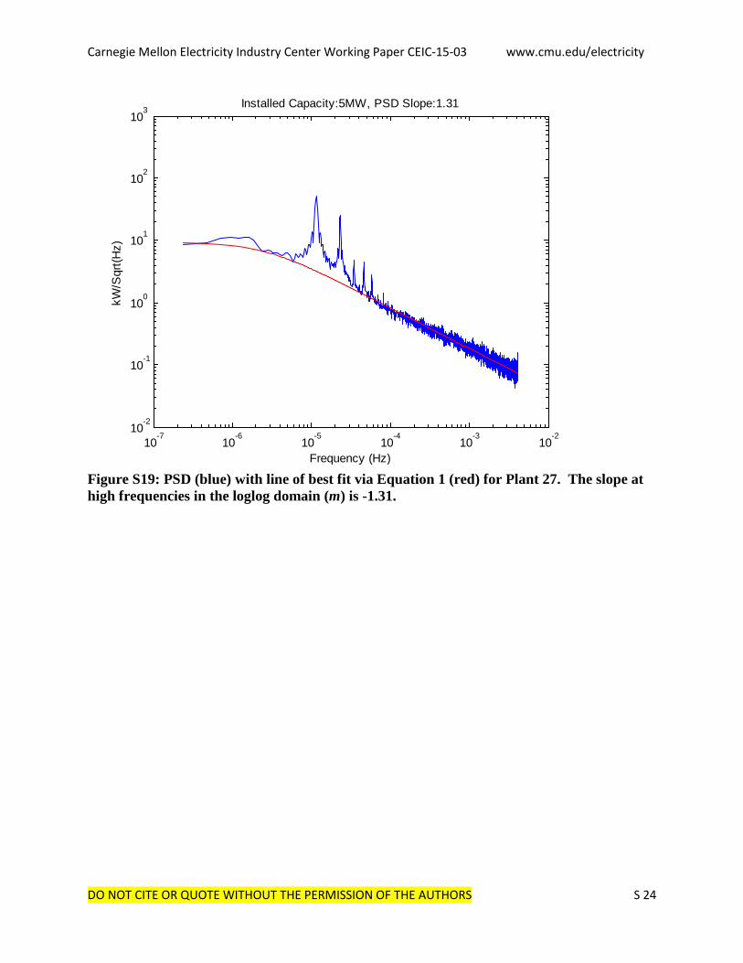
Figure S19: PSD (blue) with line of best fit via Equation 1 (red) for Plant 27. The slope at high frequencies in the loglog domain (m) is -1.31.
10-7
10-6
10-5
10-4
10-3
10-2
10-2
10-1
100
101
102
103
Frequency (Hz)
kW/S
qrt(H
z)Installed Capacity:5MW, PSD Slope:1.31
Carnegie Mellon Electricity Industry Center Working Paper CEIC-15-03 www.cmu.edu/electricity
DO NOT CITE OR QUOTE WITHOUT THE PERMISSION OF THE AUTHORS S 25
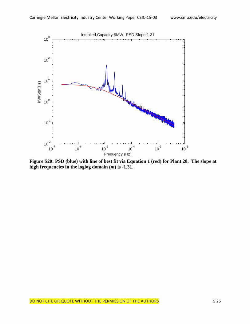
Figure S20: PSD (blue) with line of best fit via Equation 1 (red) for Plant 28. The slope at high frequencies in the loglog domain (m) is -1.31.
10-7
10-6
10-5
10-4
10-3
10-2
10-2
10-1
100
101
102
103
Frequency (Hz)
kW/S
qrt(H
z)Installed Capacity:9MW, PSD Slope:1.31

Carnegie Mellon Electricity Industry Center Working Paper CEIC-15-03 www.cmu.edu/electricity
DO NOT CITE OR QUOTE WITHOUT THE PERMISSION OF THE AUTHORS S 26
Figure S21: PSD (blue) with line of best fit via Equation 1 (red) for Plant 29. The slope at high frequencies in the loglog domain (m) is -1.27.
10-7
10-6
10-5
10-4
10-3
10-2
10-2
10-1
100
101
102
103
Frequency (Hz)
kW/S
qrt(H
z)Installed Capacity:10MW, PSD Slope:1.27

Carnegie Mellon Electricity Industry Center Working Paper CEIC-15-03 www.cmu.edu/electricity
DO NOT CITE OR QUOTE WITHOUT THE PERMISSION OF THE AUTHORS S 27
Figure S22: PSD (blue) with line of best fit via Equation 1 (red) for Plant 30. The slope at high frequencies in the loglog domain (m) is -1.24.
10-7
10-6
10-5
10-4
10-3
10-2
10-2
10-1
100
101
102
103
Frequency (Hz)
kW/S
qrt(H
z)Installed Capacity:5MW, PSD Slope:1.24

Carnegie Mellon Electricity Industry Center Working Paper CEIC-15-03 www.cmu.edu/electricity
DO NOT CITE OR QUOTE WITHOUT THE PERMISSION OF THE AUTHORS S 28
Figure S23: PSD (blue) with line of best fit via Equation 1 (red) for Plant 31. The slope at high frequencies in the loglog domain (m) is -1.35.
10-7
10-6
10-5
10-4
10-3
10-2
10-2
10-1
100
101
102
103
Frequency (Hz)
kW/S
qrt(H
z)Installed Capacity:5MW, PSD Slope:1.35
Carnegie Mellon Electricity Industry Center Working Paper CEIC-15-03 www.cmu.edu/electricity
DO NOT CITE OR QUOTE WITHOUT THE PERMISSION OF THE AUTHORS S 29
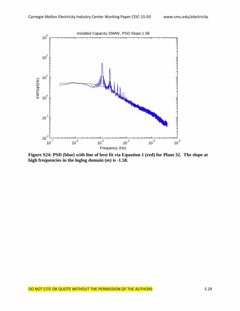
Figure S24: PSD (blue) with line of best fit via Equation 1 (red) for Plant 32. The slope at high frequencies in the loglog domain (m) is -1.58.
10-7
10-6
10-5
10-4
10-3
10-2
10-2
10-1
100
101
102
103
Frequency (Hz)
kW/S
qrt(H
z)Installed Capacity:25MW, PSD Slope:1.58

Carnegie Mellon Electricity Industry Center Working Paper CEIC-15-03 www.cmu.edu/electricity
DO NOT CITE OR QUOTE WITHOUT THE PERMISSION OF THE AUTHORS S 30
Figure S25: PSD (blue) with line of best fit via Equation 1 (red) for Plant 33. The slope at high frequencies in the loglog domain (m) is -1.45.
10-7
10-6
10-5
10-4
10-3
10-2
10-2
10-1
100
101
102
103
Frequency (Hz)
kW/S
qrt(H
z)Installed Capacity:20MW, PSD Slope:1.45
Carnegie Mellon Electricity Industry Center Working Paper CEIC-15-03 www.cmu.edu/electricity
DO NOT CITE OR QUOTE WITHOUT THE PERMISSION OF THE AUTHORS S 31
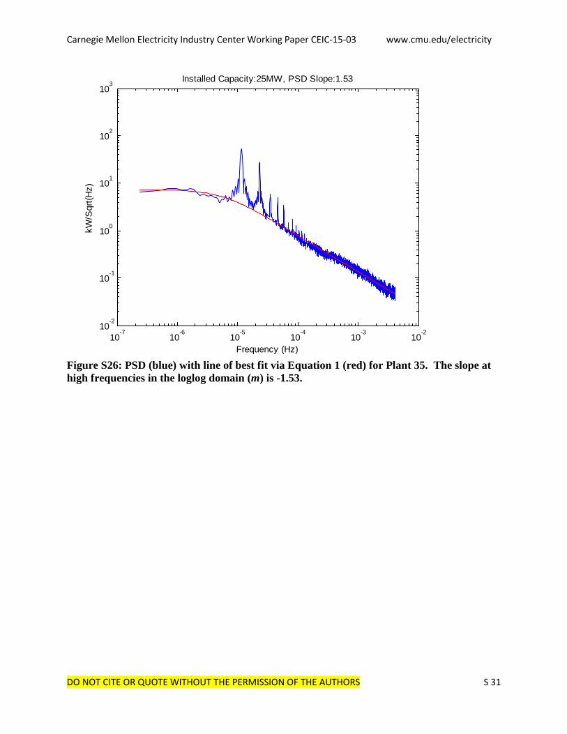
Figure S26: PSD (blue) with line of best fit via Equation 1 (red) for Plant 35. The slope at high frequencies in the loglog domain (m) is -1.53.
10-7
10-6
10-5
10-4
10-3
10-2
10-2
10-1
100
101
102
103
Frequency (Hz)
kW/S
qrt(H
z)Installed Capacity:25MW, PSD Slope:1.53
Carnegie Mellon Electricity Industry Center Working Paper CEIC-15-03 www.cmu.edu/electricity
DO NOT CITE OR QUOTE WITHOUT THE PERMISSION OF THE AUTHORS S 32
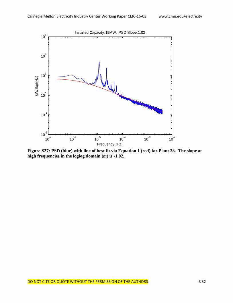
Figure S27: PSD (blue) with line of best fit via Equation 1 (red) for Plant 38. The slope at high frequencies in the loglog domain (m) is -1.02.
10-7
10-6
10-5
10-4
10-3
10-2
10-2
10-1
100
101
102
103
Frequency (Hz)
kW/S
qrt(H
z)Installed Capacity:15MW, PSD Slope:1.02

Carnegie Mellon Electricity Industry Center Working Paper CEIC-15-03 www.cmu.edu/electricity
DO NOT CITE OR QUOTE WITHOUT THE PERMISSION OF THE AUTHORS S 33
Figure S28: PSD (blue) with line of best fit via Equation 1 (red) for Plant 39. The slope at high frequencies in the loglog domain (m) is -1.24.
10-7
10-6
10-5
10-4
10-3
10-2
10-2
10-1
100
101
102
103
Frequency (Hz)
kW/S
qrt(H
z)Installed Capacity:15MW, PSD Slope:1.24

Carnegie Mellon Electricity Industry Center Working Paper CEIC-15-03 www.cmu.edu/electricity
DO NOT CITE OR QUOTE WITHOUT THE PERMISSION OF THE AUTHORS S 34
Figure S29: PSD (blue) with line of best fit via Equation 1 (red) for Plant 40. The slope at high frequencies in the loglog domain (m) is -1.29.
10-7
10-6
10-5
10-4
10-3
10-2
10-2
10-1
100
101
102
103
Frequency (Hz)
kW/S
qrt(H
z)Installed Capacity:5MW, PSD Slope:1.29
Carnegie Mellon Electricity Industry Center Working Paper CEIC-15-03 www.cmu.edu/electricity
DO NOT CITE OR QUOTE WITHOUT THE PERMISSION OF THE AUTHORS S 35
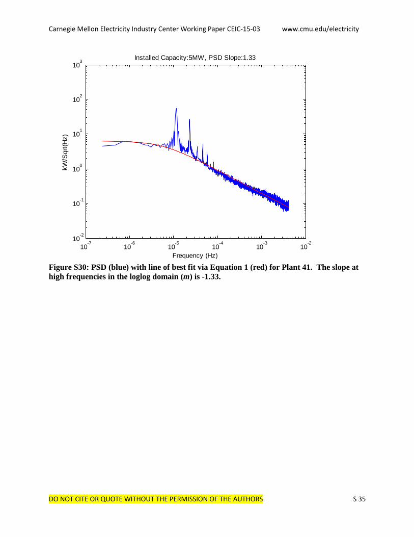
Figure S30: PSD (blue) with line of best fit via Equation 1 (red) for Plant 41. The slope at high frequencies in the loglog domain (m) is -1.33.
10-7
10-6
10-5
10-4
10-3
10-2
10-2
10-1
100
101
102
103
Frequency (Hz)
kW/S
qrt(H
z)Installed Capacity:5MW, PSD Slope:1.33
Carnegie Mellon Electricity Industry Center Working Paper CEIC-15-03 www.cmu.edu/electricity
DO NOT CITE OR QUOTE WITHOUT THE PERMISSION OF THE AUTHORS S 36
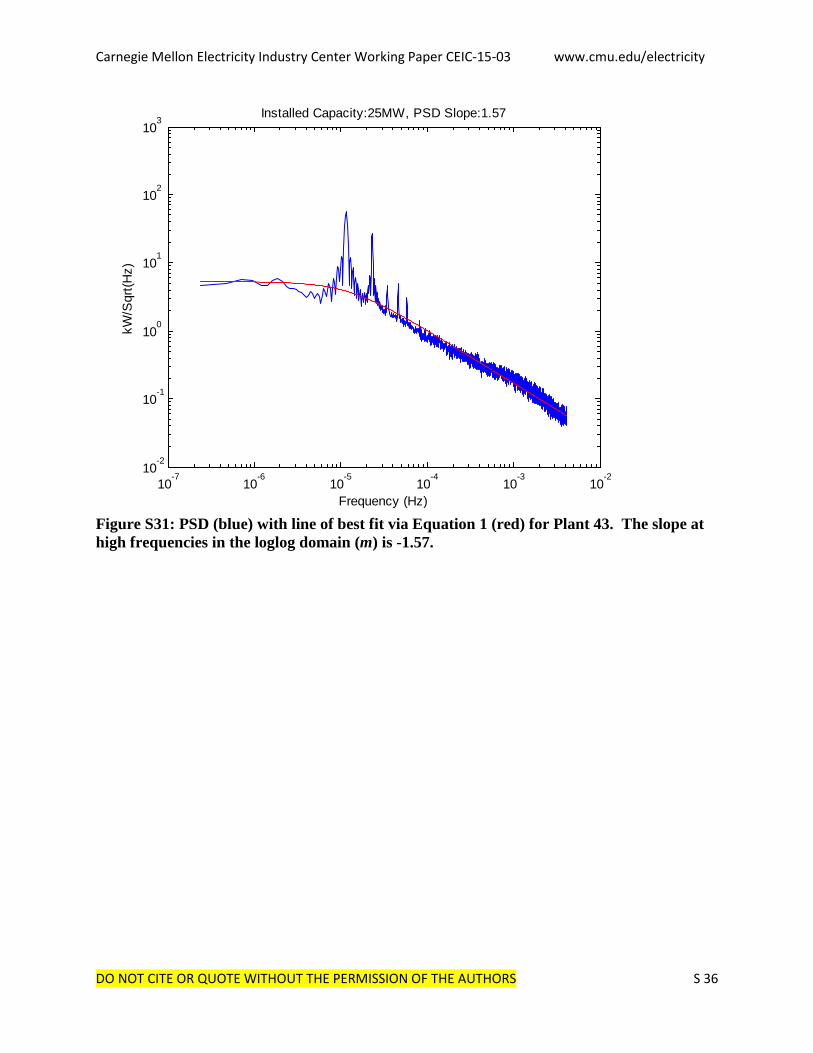
Figure S31: PSD (blue) with line of best fit via Equation 1 (red) for Plant 43. The slope at high frequencies in the loglog domain (m) is -1.57.
10-7
10-6
10-5
10-4
10-3
10-2
10-2
10-1
100
101
102
103
Frequency (Hz)
kW/S
qrt(H
z)Installed Capacity:25MW, PSD Slope:1.57

Carnegie Mellon Electricity Industry Center Working Paper CEIC-15-03 www.cmu.edu/electricity
DO NOT CITE OR QUOTE WITHOUT THE PERMISSION OF THE AUTHORS S 37
Figure S32: PSD (blue) with line of best fit via Equation 1 (red) for Plant 44. The slope at high frequencies in the loglog domain (m) is -1.52.
10-7
10-6
10-5
10-4
10-3
10-2
10-2
10-1
100
101
102
103
Frequency (Hz)
kW/S
qrt(H
z)Installed Capacity:25MW, PSD Slope:1.52

Carnegie Mellon Electricity Industry Center Working Paper CEIC-15-03 www.cmu.edu/electricity
DO NOT CITE OR QUOTE WITHOUT THE PERMISSION OF THE AUTHORS S 38
Figure S33: PSD (blue) with line of best fit via Equation 1 (red) for Plant 45. The slope at high frequencies in the loglog domain (m) is -1.29.
10-7
10-6
10-5
10-4
10-3
10-2
10-2
10-1
100
101
102
103
Frequency (Hz)
kW/S
qrt(H
z)Installed Capacity:5MW, PSD Slope:1.29

Carnegie Mellon Electricity Industry Center Working Paper CEIC-15-03 www.cmu.edu/electricity
DO NOT CITE OR QUOTE WITHOUT THE PERMISSION OF THE AUTHORS S 39
Figure S34: PSD (blue) with line of best fit via Equation 1 (red) for Plant 47. The slope at high frequencies in the loglog domain (m) is -1.27.
10-7
10-6
10-5
10-4
10-3
10-2
10-2
10-1
100
101
102
103
Frequency (Hz)
kW/S
qrt(H
z)Installed Capacity:5MW, PSD Slope:1.27
Carnegie Mellon Electricity Industry Center Working Paper CEIC-15-03 www.cmu.edu/electricity
DO NOT CITE OR QUOTE WITHOUT THE PERMISSION OF THE AUTHORS S 40
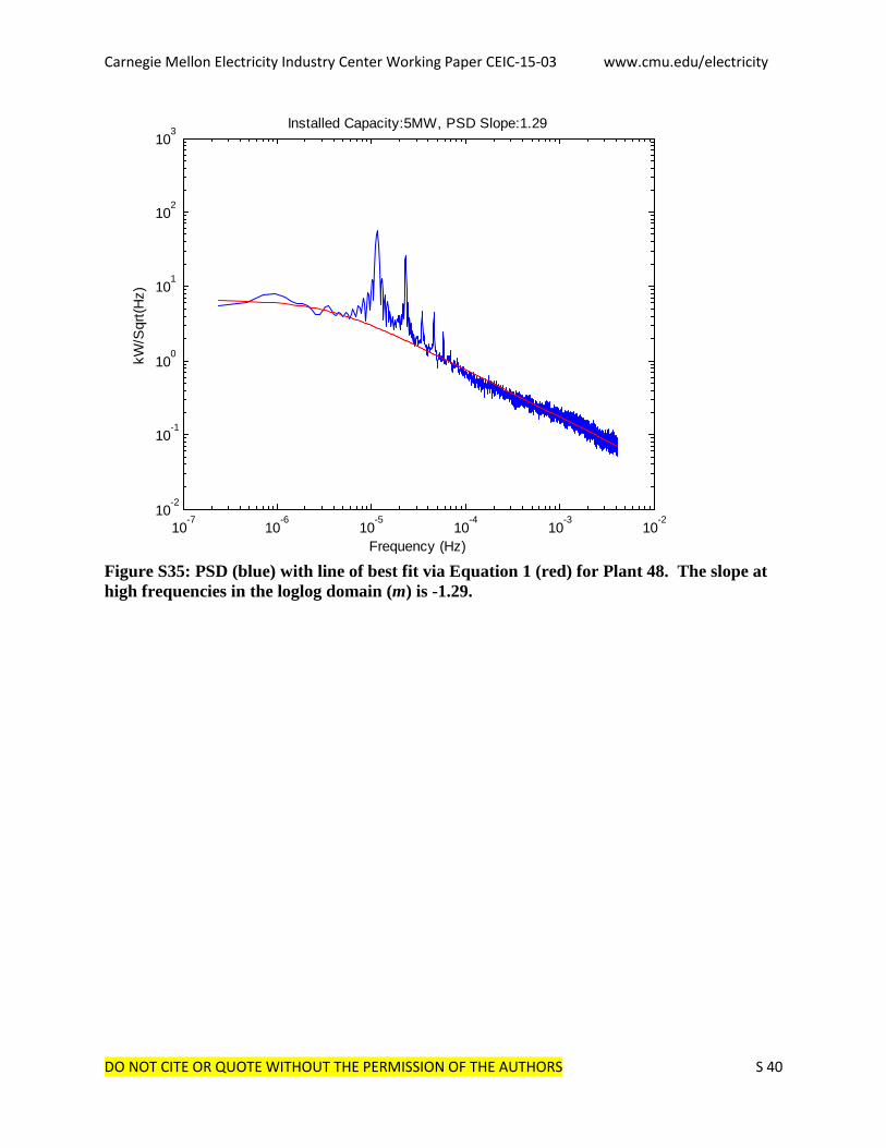
Figure S35: PSD (blue) with line of best fit via Equation 1 (red) for Plant 48. The slope at high frequencies in the loglog domain (m) is -1.29.
10-7
10-6
10-5
10-4
10-3
10-2
10-2
10-1
100
101
102
103
Frequency (Hz)
kW/S
qrt(H
z)Installed Capacity:5MW, PSD Slope:1.29

Carnegie Mellon Electricity Industry Center Working Paper CEIC-15-03 www.cmu.edu/electricity
DO NOT CITE OR QUOTE WITHOUT THE PERMISSION OF THE AUTHORS S 41
Figure S36: PSD (blue) with line of best fit via Equation 1 (red) for 221MW plant. The slope at high frequencies in the loglog domain (m) is -1.76.
10-7
10-6
10-5
10-4
10-3
10-2
10-2
10-1
100
101
102
103
Frequency (Hz)
kW/S
qrt(H
z)Installed Capacity:221MW, PSD Slope:1.76

Carnegie Mellon Electricity Industry Center Working Paper CEIC-15-03 www.cmu.edu/electricity
DO NOT CITE OR QUOTE WITHOUT THE PERMISSION OF THE AUTHORS S 42
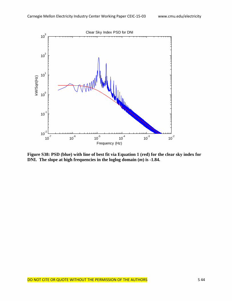
4. Power spectral densities calculated using the Lomb periodiogram for Clear Sky Index For reference, we calculated the Bird and Hulstrom Clear Sky Index for direct normal irradiance upon a horizontal surface and global horizontal irradiance upon a horizontal surface [7] for Plant 50 (Charanka) for 1-minute resolution for one year. The slope of both of these models is -1.84 at high frequencies.

Carnegie Mellon Electricity Industry Center Working Paper CEIC-15-03 www.cmu.edu/electricity
DO NOT CITE OR QUOTE WITHOUT THE PERMISSION OF THE AUTHORS S 43
Figure S37: PSD (blue) with line of best fit via Equation 1 (red) for the clear sky index for GHI. The slope at high frequencies in the loglog domain (m) is -1.84.
10-7
10-6
10-5
10-4
10-3
10-2
10-2
10-1
100
101
102
103
Frequency (Hz)
kW/S
qrt(H
z)Clear Sky Index PSD for GHI
Carnegie Mellon Electricity Industry Center Working Paper CEIC-15-03 www.cmu.edu/electricity
DO NOT CITE OR QUOTE WITHOUT THE PERMISSION OF THE AUTHORS S 44
Figure S38: PSD (blue) with line of best fit via Equation 1 (red) for the clear sky index for DNI. The slope at high frequencies in the loglog domain (m) is -1.84.
10-7
10-6
10-5
10-4
10-3
10-2
10-2
10-1
100
101
102
103
Frequency (Hz)
kW/S
qrt(H
z)Clear Sky Index PSD for DNI
Carnegie Mellon Electricity Industry Center Working Paper CEIC-15-03 www.cmu.edu/electricity
DO NOT CITE OR QUOTE WITHOUT THE PERMISSION OF THE AUTHORS S 45
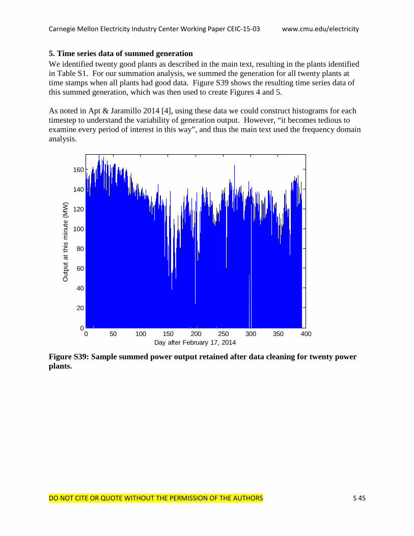
5. Time series data of summed generation We identified twenty good plants as described in the main text, resulting in the plants identified in Table S1. For our summation analysis, we summed the generation for all twenty plants at time stamps when all plants had good data. Figure S39 shows the resulting time series data of this summed generation, which was then used to create Figures 4 and 5. As noted in Apt & Jaramillo 2014 [4], using these data we could construct histograms for each timestep to understand the variability of generation output. However, “it becomes tedious to examine every period of interest in this way”, and thus the main text used the frequency domain analysis.
Figure S39: Sample summed power output retained after data cleaning for twenty power plants.
0 50 100 150 200 250 300 350 4000
20
40
60
80
100
120
140
160
Day after February 17, 2014
Out
put a
t thi
s m
inut
e (M
W)
Carnegie Mellon Electricity Industry Center Working Paper CEIC-15-03 www.cmu.edu/electricity
DO NOT CITE OR QUOTE WITHOUT THE PERMISSION OF THE AUTHORS S 46
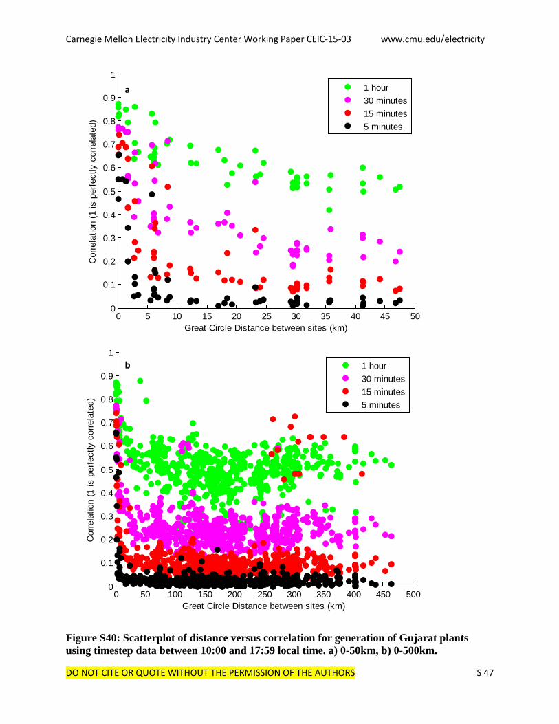
6. Scatterplot of distance versus correlation for the Gujarat plant generations To understand the potential for smoothing, many studies have examined correlation versus distance. Most use either a clear sky index or a method to remove the diurnal cycle, and find that correlation decreases to 0 as distance increases [8, 9, 10, 11, 12]. This approach allows one to understand cloud variability, which is of importance to power plant operators. However, power plant generation is a function of both the clear sky index and the solar signal, and thus to make siting decisions, a systems operator would likely prefer a study of generation data such as the one presented in the main text. We identified two studies examining distance versus correlation of irradiance data that did not remove the diurnal cycle. A study in Oklahoma, United States of America showed that as distance increases, correlation decreases but not to 0 (see Figure 6 in Barnett et al. 1998) [13]. Similarly, a study in Ontario, Canada (see Figure 2 in Rowlands et al., 2013) [14] shows that as distance increases, correlation decreases and asymptotes at a nonegative value. These findings align with the qualitative discussion in Mills et al. 2009 [15]. To understand whether these findings might hold true for generation data, we calculated distance versus correlation for power plant generation. We first calculated ramp data (difference in generation between timesteps) between 10:00 and 17:59 local time. We then interpolated these data to even one-minute timesteps, then decimated the values to 5, 15, 30, and 60 minute timesteps (thus accounting for selection bias). Figure S40 shows a decrease in correlation as distance between plants increases toward 50km. Near 100km, the correlation becomes almost constant as a function of distance, as one might expect with the correlation in the solar cycle. These findings agree with the previous results examining distance versus correlation of irradiance data. We next considered attempting to remove the solar cycle signal to attempt to replicate studies using clear sky indices and thus understand the potential for smoothing. However, it is very difficult to remove this signal since it is a complex function of hour, day, season, and year. Thus in the main text, we used a frequency domain method.
Carnegie Mellon Electricity Industry Center Working Paper CEIC-15-03 www.cmu.edu/electricity
DO NOT CITE OR QUOTE WITHOUT THE PERMISSION OF THE AUTHORS S 47
0 5 10 15 20 25 30 35 40 45 500
0.1
0.2
0.3
0.4
0.5
0.6
0.7
0.8
0.9
1
Great Circle Distance between sites (km)
Cor
rela
tion
(1 is
per
fect
ly c
orre
late
d)
1 hour30 minutes15 minutes5 minutes
Figure S40: Scatterplot of distance versus correlation for generation of Gujarat plants using timestep data between 10:00 and 17:59 local time. a) 0-50km, b) 0-500km.
0 50 100 150 200 250 300 350 400 450 5000
0.1
0.2
0.3
0.4
0.5
0.6
0.7
0.8
0.9
1
Great Circle Distance between sites (km)
Cor
rela
tion
(1 is
per
fect
ly c
orre
late
d)
1 hour30 minutes15 minutes5 minutes
a
b
Carnegie Mellon Electricity Industry Center Working Paper CEIC-15-03 www.cmu.edu/electricity
DO NOT CITE OR QUOTE WITHOUT THE PERMISSION OF THE AUTHORS S 48
References 1 SLDC-Gujarat. “State Load Despatch Centre (SLDC) – Real-Time System Data”. https://www.sldcguj.com/RealTimeData/GujSolar.asp Accessed by authors every minute from February 17, 2014 to March 16, 2015. 2 UNFCCC. “CDM: CDM-Home”. http://cdm.unfccc.int/ Accessed April 13, 2015. 3 Curtright, A.E.; Apt, J. (2008). The character of power output from utility-scale photovoltaic systems. Progress in Photovoltaics: Research and Applications. 16(3), 241–247. 4 Apt, J.; Jaramillo, P. Variable Renewable Energy and the Electricity Grid. RFF Press: Oxford, 2014. 5 Lueken, C.; Cohen, G.E.; Apt, J. (2012). Costs of solar and wind power variability for reducing CO2 emissions. Environmental Science & Technology. 46(1), 9761-9767. 6 Marco s, J.; Marroyo, L.; Lorenzo, E.; Alvira, E.; Izco, E. (2011). From Irradiance to Output Power Fluctuations: The PV Plant as a Low Pass Filter. Progress in Photovoltaics: Research and Applications. 19(5), 505–10. 7 Bird, R.E.; Hulstrom, R.L. (1991). A Simplified Clear Sky Model for Direct and Diffuse Insolation on Horizontal Surfaces. SERI Technical Report SERI/TR-642-761. Solar Energy Research Institute, Golden, CO. 8 Kleissel, Jan (2013). Solar Energy Forecasting and Resource Assessment. Academic Press: Amsterdam. 9 Long, C.N.; Ackerman, T.P. (1995). Surface Measurements of Solar Irradiance: A Study of the Spatial Correlation between Simultaneous Measurements at Separated Sites. Journal of Applied Meteorology. 34(1), 1039–1046. 10 Lave, M.; Kleissl, J. (2010). Solar variability of four sites across the state of Colorado. Renewable Energy. 35(12), 2867–2873. 11 Otani, K.; Minowa, J.; Kurokawa, K. (1997). Study on area solar irradiance for analyzing areally‐totalized PV systems. Solar Energy Materials and Solar Cells. 47(1), 281‐288. 12 Lave, M.; Kleissl, J.; Arias-Castro, E. (2012). High-frequency irradiance fluctuations and geographic smoothing. Solar Energy. 86(8), 2190–2199. 13 Barnett, T.P.; Ritchie, J.; Foat, J.; Stokes, G. (1998). On the Space–Time Scales of the Surface Solar Radiation Field. Journal of Climate. 11(1), 88–96. 14 Rowlands, I.H.; Kemery, B.P.; Beausoleil-Morrison, I. (2014). Managing solar-PV variability with geographical dispersion: An Ontario (Canada) case-study. Renewable Energy. 68(1), 171–180. 15 Mills, A.D.; Wiser, R.H. (2010). Implications of Wide-Area Geographic Diversity for Short- Term Variability of Solar Power. Technical Report LBNL-3884E.