Smoothing and forecasting mortality rates

Running headline: Smoothing and forecasting mortality rates

I D Currie, Department of Actuarial Mathematics and Statistics, Heriot-Watt University,

Edinburgh, EH14 4AS, UK.

M Durban, Departamento de Estadistica y Econometria, Universidad Carlos III de Madrid,

Edificio Torres Quevedo, 28911 Leganes, Madrid, Spain.

P H C Eilers, Department of Medical Statistics, Leiden University Medical Center,

2300 RC Leiden, The Netherlands.

Responsible author: I D Currie, Email: I.D.Currie@hw.ac.uk

Abstract: The prediction of future mortality rates is a problem of fundamental importance

for the insurance and pensions industry. We show how the method of P -splines (Eilers and

Marx, 1996) can be extended to the smoothing and forecasting of two-dimensional mortality

tables. We use a penalized generalized linear model (PGLM) with Poisson errors and show how

to construct regression and penalty matrices appropriate for two-dimensional modelling. An

important feature of our method is that forecasting is a natural consequence of the smoothing

process. We illustrate our methods with two data sets provided by the Continuous Mortality

Investigation Bureau (CMIB), a central body for the collection and processing of UK insurance

and pensions data.

Keywords: Forecasting; mortality; overdispersion; P -splines; two dimensions.

1

1 Introduction

The modelling and projecting of disease incidence and mortality rates is a problem of funda-

mental importance in epidemiology and population studies generally, and for the insurance and

pensions industry in particular. Human mortality has improved substantially over the last cen-

tury but this manifest benefit has brought with it additional stress in support-systems for the

elderly, such as health-care and pension provision. For the insurance and pensions industry the

pricing and reserving of annuities depends on three things: stock market returns, interest rates

and future mortality rates. Likewise, the return from savings for the policyholder depends on

the same three factors. In the most obvious way, increasing longevity can only be regarded as a

good thing for the policyholder; a less welcome consequence is that annual income from annuities

will be reduced. In this paper we consider one of these three factors: the prediction of mortality

rates. We have been provided with data sets from two classes of UK insurance business and we

will use these to illustrate our approach to the smoothing and projecting of mortality rates.

The requirements of the insurance industry for forecasts of future mortality are daunting

indeed, since forecasts up to fifty years ahead are required for pricing and reserving. Human

mortality so far ahead depends on the impact of such unknowables as future medical advances,

new infectious diseases, and even disasters, both natural and man-made. We make no attempt

to take these factors into account and instead simply attempt to forecast future mortality by

extrapolating past trends. There are a number of approaches to the problem. One of the oldest

methods is based on the forecasting of parameters in some parametric model. For example,

Age-Period-Cohort (APC) models are a well established method of smoothing mortality tables.

The classic reference is Clayton and Schifflers (1987). These authors sound warnings about the

dangers of over-interpreting the fitted parameters in an APC model and are equally sceptical

about the wisdom of extrapolating. Lee and Carter (1992) introduced a simple bilinear model of

mortality in which the time dependent component of mortality is reduced to a single index which

is then forecast using time series methods. The model is fitted by ordinary least squares (OLS)

with the observed log mortality rates as dependent variable. Brouhns et al. (2002) improved

on the OLS approach by modelling the number of deaths directly by a Poisson distribution and

using maximum likelihood for parameter estimation.

Both the APC and the Lee-Carter approach make strong assumptions about the functional

form of the mortality surface. There are various fully two-dimensional approaches. Loess (Cleve-

land and Devlin, 1988) is available directly in the gam( ) function in Splus/R but does not allow

2

extrapolation. De Boor (2001) and Dierckx (1993) construct a two-dimensional regression ba-

sis as the Kronecker product of B-splines but neither author considers non-normal data or the

forecasting problem. Gu and Wahba (1993) and Wood (2003) use thin plate splines but again

forecasting is not available. Our own approach is to use two-dimensional regression splines,

specifically B-splines with penalties, usually known as P -splines (Eilers and Marx, 1996). This

approach is used in Eilers and Marx (2003) and Eilers et al. (2004) but neither paper considers

forecasting.

Eilers and Marx (1996) used B-splines as a basis for one-dimensional regression and we extend

this work by using B-splines to construct a basis for bivariate regression. This construction gives

a basis in two dimensions with local support and hence a fully flexible family of fitted mortality

surfaces. The regression approach leads to a generalized linear model which is fitted by penalized

likelihood. An important feature of this method is that forecasting is a natural consequence of

the smoothing process. We consider future values as missing values; the penalization then allows

estimation of the future values simultaneously with the fitting of the mortality surface. We will

see that the choice of penalty function, which can be of secondary importance in the smoothing

of data, is now critical, since it is the penalty function that determines the form of the forecast.

The plan of the paper is as follows. In section 2 we describe our two data sets. In section 3

we review the P -spline approach in one dimension and then show how this extends to two

dimensions; the missing value approach to forecasting is also described. In section 4 we apply

our methods to our two data sets; overdispersion is a particular problem with one of the data

sets and we describe one way of dealing with this problem. The paper concludes with a critical

discussion of our methodology and the implications of the findings for the UK insurance industry.

2 Description of the data

The mortality of insured lives differs from that of the general population and even differs within

different classes of business. The Continuous Mortality Investigation Bureau (CMIB) is a central

body funded by the UK insurance and pensions industry. UK insurance companies submit claims

data to the CMIB for collation and analysis, the principal aim of which is the forecasting of

age-specific mortality tables for various classes of insured lives. In this paper we consider two of

the CMIB data sets, one for male assured lives and one for male pensioners. We describe each

of these data sets in turn.

3

Male assured lives. For each calendar year (1947 to 1999) and each age (11 to 100) we have

the number of policy claims (deaths) and the number of years lived (the exposure). The claims

and exposure data are arranged respectively in matrices Y and E whose rows are indexed by

age (here 11 to 100) and whose columns are indexed by year (here 1947 to 1999). One possible

difficulty with the data is that claims do not correspond precisely to deaths since an individual

life may hold more than one policy and thus give rise to more than one claim. This is known as

the problem of duplicates in insurance terminology and leads to the statistical phenomenon of

overdispersion. It is convenient to define R = Y /E, the matrix of raw hazards. The problem is

to project values of the underlying hazard forward in time.

Male pensioners. This data set is richer than the previous set since in addition to data Y

and E as above we also have matching data Z and F on amounts. To be precise, the claims

in Y give rise to total amounts claimed in Z and the exposures E give rise to total amounts

at risk F . These data are available for calendar years 1983 to 2000 and ages 50 to 100. We

define RL = Y /E, the matrix of raw hazards based on lives, and RA = Z/F , the corresponding

quantity based on amounts; here, and below, the suffices L and A indicate lives and amounts

respectively. Clearly if all policies are for the same amount then RL = RA. In practice this

is very far from the case, and it is generally found that RA < RL, i.e., the mortality of those

lives with larger policy amounts is better than those with smaller amounts. The problem of

duplicates which is present to a small degree in lives data is an essential feature of amounts

data, since the variation between amounts at risk contributes directly to the variation in the

total amounts claimed.

3 Smoothing and forecasting mortality tables with P -splines

The method of P -splines is now well established as a method of smoothing in generalized linear

models (GLMs). Descriptions of the method can be found in the original paper of Eilers and

Marx (1996) as well as in Marx and Eilers (1998), Eilers and Marx (2002), Currie and Durban

(2002) and elsewhere. Wand’s (2003) review paper adopts a mixed model approach and provides

a useful bibliography. Theoretical aspects of P -splines are discussed in Wand (1999), Ruppert

and Carroll (2000), Aerts et al. (2002), Ruppert (2002), and Durban and Currie (2003). Papers

which emphasise applications include Marx and Eilers (1999), Parise et al. (2001), Coull et al.

(2001a, 2001b), and Currie and Durban (2002). Wood and Augustin (2002) and Wood (2003)

also use penalized regression but with a different basis from that of the present approach.

4

A succinct summary of the method of P -splines is: (a) use B-splines as the basis for the

regression, and (b) modify the log-likelihood by a difference penalty on the regression coefficients.

It is usual to think of smoothing in GLMs in the GAM framework but we find it helpful to think

of the method as a penalized generalized linear model (PGLM). There are two reasons for

this: model building and computation. In a PGLM we define a regression matrix, an error

distribution, a link function (GLM) and additionally a penalty matrix; computationally our

method extends the GLM scoring algorithm but retains the iterative weighted least squares

form. Eilers and Marx (1996) showed how to smooth Poisson data in one dimension. We extend

their method to two dimensions by constructing regression and penalty matrices appropriate

for two-dimensional modelling. This section is divided into four: 3.1, the basic one-dimensional

model and the choice of the various parameters implicit in smoothing with P -splines; 3.2, the

definition of the two-dimensional regression matrix; 3.3, the definition of the penalty matrix;

and finally 3.4, the method of extrapolation.

3.1 Smoothing in one dimension

For the benefit of readers unfamiliar with smoothing using P -splines we present a short intro-

duction to the method. We suppose we have data (yi, ei, xi), i = 1, . . . , n, on a set of lives

all aged 65, say, where yi is the number of deaths in year xi and ei is the exposed to risk. Let

y′ = (y1, . . . , yn), e′ = (e1, . . . , en), etc. We suppose that the number of deaths yi is a realization

of a Poisson distribution with mean µi = eiθi. For an introduction to P -splines with normal

errors see, for example, Eilers and Marx (1996) or Marx and Eilers (1998). The left hand panel

of Figure 1 shows a plot of the logarithm of the raw forces of mortality, θi = yi/ei. We seek

a smooth estimate of θ = (θi). A classical approach might be to fit a generalized linear model

(GLM) with quadratic regression term, i.e., log µ = log e + log θ = log e + Xa where log e is

an offset in the regression term; the result is shown in the left hand panel. This simple model

uses {1, x, x2} as basis functions. A more flexible basis is provided by a set of cubic B-splines

{B1(x), . . . , BK(x)} and such a basis is shown for K = 8 in the right panel of Figure 1; each

B-spline consists of cubic polynomial pieces smoothly bolted together at points known as knots.

We are still in the framework of classical regression with regression matrix, B, say. The rows of

B are the values of the B-splines in the basis evaluated at each year in turn; thus, for example,

the estimate of log θ at 1970 is

0.0817 × a3 + 0.6267 × a4 + 0.2901 × a5 + 0.0016 × a6, (3.1)

5

••••

•

•

••

••••

•••

•••••

••

•

•••

••••

••••••••

•

•••••

•••

•

•••••

Year

log(m

orta

lity)

1950 1970 1990

-4.6

-4.4

-4.2

-4.0

-3.8

-3.6

Age 65

Year

B-sp

line

1950 1970 1990

0.0

0.2

0.4

0.6

• • • • • •

1

23 4 5 6

7

8

Figure 1: Left panel: Observed log(mortality) and fitted quadratic linear predictor; right panel:a basis of K = 8 cubic B-splines with knots

as can be seen from the dashed line in the right panel of Figure 1. In general B1 = 1, B ≥ 0

and B is a banded matrix, so the fitted values Ba are weighted averages of local subsets of the

coefficients; interestingly enough, the same weights applied to the knot positions k recover the

x values since Bk = x.

The left panel of Figure 2 shows the result of fitting a GLM with K = 23 B-splines in

the basis. Evidently the data have been undersmoothed. The plot also shows the regression

coefficients (a2, . . . , a22) plotted at the maximum value of their corresponding B-spline (a1 =

−3.05 and a23 = −2.45 are omitted since their extreme values distort the scale of the plot).

Eilers and Marx (1996) observed that the undersmoothing in the left panel of Figure 2 was a

result of the erratic behaviour of the ak and they proposed penalizing this behaviour by placing

a difference penalty on adjacent ak, as in

(a1 − 2a2 + a3)2 + . . . + (aK−2 − 2aK−1 + aK)2 = a′D′Da (3.2)

where D is a difference matrix of order 2; this defines a quadratic penalty but linear and cubic

penalty functions are also possible. The penalty function is incorporated into the log likelihood

6

Year

Log(

mor

tality

)

1950 1970 1990

-4.8

-4.4

-4.0

-3.6

••••

•

•

••••••

••••••••

••

•

••••••••••••

••••

••••••••

••••••Age = 65

Npar = 23DF = 23

Year

1950 1970 1990

-4.8

-4.4

-4.0

-3.6

••••

•

•

••••••

•••

•••••

••

•

••••••••••••

•••

•

••••••••

••••••Age = 65

Npar = 23

DF = 6.0

Figure 2: Left panel: Observed log(mortality), fitted regression with a basis of K = 23 cubicB-splines and regression coefficients, ◦; right panel: as left panel but with P -spline regression.Knot positions are shown by vertical tick marks.

function to give the penalized log likelihood

`p = `(a; y) − 12a′Pa (3.3)

= `(a; y) − 12λa′D′Da (3.4)

where `(a; y) is the usual log likelihood for a GLM, P = λD′D is the penalty matrix and λ is

the smoothing parameter.

Maximizing (3.3) gives the penalized likelihood equations

B′(y − µ) = Pa (3.5)

which can be solved with the penalized version of the scoring algorithm

(B′WB + P )a = B′WBa + B′(y − µ) (3.6)

where B is the regression matrix, P is the penalty matrix, a, µ and W , the diagonal matrix of

weights, denote current estimates, and a denotes the updated estimate of a. Notice that (3.5)

and (3.6) are the standard likelihood equations and scoring algorithm respectively for a GLM

adjusted for the quadratic term in (3.3). Note that (3.6) corrects a misprint in equation (16) in

7

Eilers and Marx (1996). In the case of Poisson errors, we have W = diag(µ). The algorithm

(3.6) can also be written as

(B′WB + P )a = B′W z (3.7)

where z = η + W−1

(y − µ) which emphasizes the connection between this algorithm and the

standard iterative weighted least squares algorithm for a GLM.

It follows from (3.7) that the hat-matrix is given by

H = B(B′WB + P )−1B′W (3.8)

and the trace of the hat-matrix, tr(H), is a measure of the effective dimension or degrees of

freedom of the model; see Hastie and Tibshirani (1990, p52). The approximate variance of Ba

is given by

Var(Ba) ≈ B(B′WB + P )−1B′. (3.9)

One justification of (3.9) is that the P -spline estimator of Ba can be derived from a Bayesian

perspective and (3.9) coincides with its Bayesian variance; see Lin and Zhang (1999).

The user of P -splines has a number of choices to make: (a) the number of knots, the degree

of the P -spline and the order of the penalty, and (b) the smoothing parameter. The parameters

in (a) we call the P -spline parameters and denote them by ndx, bdeg and pord respectively. We

will see that when forecasting with P -splines the forecast values depend critically on the order

of the penalty. The choice of the other P -spline parameters, ndx and bdeg, can be less critical

since different choices often lead to similar fitted smooth functions. Eilers and Marx (1996),

Ruppert (2002) and Currie and Durban (2002) discuss the choice of the P -spline parameters;

the following simple rule-of-thumb is often sufficient: with equally spaced data, use one knot

for every four or five observations up to a maximum of forty knots to guide the choice of the

number of knots parameter, ndx, (strictly ndx−1 is the number of internal knots in the domain

of x); use cubic splines (bdeg = 3) and a quadratic penalty (pord = 2).

We will use the Bayesian Information Criterion, BIC, (Schwarz, 1978) to choose the smooth-

ing parameter where

BIC = 2 Dev + log n Tr; (3.10)

here Dev is the deviance in a GLM, Tr = tr(H) is the effective dimension of the fitted model,

as in (3.8), and n is the number of observations. Other possibilities are AIC or GCV but there

is evidence that AIC and GCV tend to undersmooth the data; see, for example, Hurvich et al.

(1998) or Lee (2003). BIC penalizes model complexity more heavily than AIC particularly, as in

8

our examples, when n is large. See Chatfield (2003) for a useful discussion on criteria for model

choice. An alternative approach is to express the PGLM as a generalized linear mixed model

(GLMM) and this also leads to an estimate of the smoothing parameter.

The right panel of Figure 2 shows the result of fitting the PGLM. The P -spline parameters

were: bdeg = 3 (cubic B-splines), pord = 2 (second order penalty) and ndx = 20 which gives

K = ndx + bdeg = 23 B-splines in the basis. The optimal value of the smoothing parameter,

λ = 3900, was chosen via BIC. This level of smoothing has the effect of reducing the degrees of

freedom from 23 (the number of fitted parameters) to about 6.

We close this introduction with a few general comments about the method of P -splines. The

method has a number of attractive features. First, the method is an example of a low-rank

smoother, since the order of the system of equations (3.6) is equal to the number of B-splines in

the basis, and this is generally much less than the number, n, of data points (smoothing splines

use matrices of order n). Second, the algorithm (3.6) or (3.7) is computationally efficient since

it is essentially the same as the iterative weighted least squares (IWLS) algorithm used to fit

a GLM. Third, the regression form for the mean (log µ = log e + Ba in our example) makes

regression-style model-building straightforward (see section 4.2 for an example).

3.2 Two-dimensional regression matrix

One of the principal motivations behind the use of B-splines as the basis of regression is that it

does not suffer from the lack of stability that can so bedevil ordinary polynomial regression. The

essential difference is that B-splines have local non-zero support in contrast to the polynomial

basis for standard regression. We seek to construct a basis for two-dimensional regression with

local support analogous to the way that B-splines provide a basis for one-dimensional regression.

Suppose we have a two-dimensional regression problem with regression variables x1 and x2

where the data Y are available over an m × n grid; the rows of Y are indexed by x1 and

the columns by x2 (age and year respectively in our example). For the purpose of regression

we suppose that the data are arranged in column order, i.e., y = vec(Y ). Consider a simple

polynomial model with linear predictor defined by 1 + x1 + x2 + x22 + x1x2 + x1x

22. Let X be

the regression matrix for this model. Now consider two one-dimensional models, one in x1 for a

column yc of Y and one in x2 for a row yr of Y . Let X1 be the regression matrix corresponding

to the model with linear predictor 1 + x1 and, in a similar fashion, let X2 be the regression

matrix corresponding to the model with linear predictor 1+x2 +x22. We observe that the model

9

formula 1 + x1 + x2 + x22 + x1x2 + x1x

22 factorises into (1 + x2 + x2

2)(1 + x1) and it follows that

X = X2 ⊗ X1, (3.11)

as may be easily checked directly. Here ⊗ denotes the Kronecker product of two matrices; see

Searle (1982, p265).

We refer to a model for a column or row of Y as a marginal model. Thus (3.11) says that the

regression matrix for a polynomial regression in x1 and x2, whose model formula can be written

as the product of two marginal models, can be written as the Kronecker product of the regression

matrices of the marginal models. In ordinary two-dimensional regression this observation seems

little more than a curiosity but we use exactly this idea to produce a two-dimensional regression

matrix with local support. Let Ba = B(xa), na × ca, be a regression matrix of B-splines based

on the explanatory variable for age xa and similarly, let By = B(xy), ny × cy, be a regression

matrix of B-splines based on the explanatory variable for year xy. The regression matrix for

our two-dimensional model is the Kronecker product

B = By ⊗ Ba. (3.12)

This formulation assumes that the vector of observed claim numbers y = vec(Y ), (this corre-

sponds to how Splus stores a matrix). In the case of assured lives, the data are on a 90 × 53

grid, and the matrices Ba and By are typically 90× 20 and 53× 10 when B will be 4770× 200.

Figure 3 gives a feel for what a Kronecker product basis looks like. The age-year grid is

populated by a set of overlapping hills which are placed at regular intervals over the region.

Each hill is the Kronecker product of two one-dimensional hills (B-splines), one in age and one

in year. For clarity, only a subset of hills from a small basis is shown in Figure 3, but in practice

there are about 200 such hills which give a dense covering of the age-year region, and this results

in a flexible basis for two-dimensional regression.

3.3 Two-dimensional penalty matrix

The regression matrix B = By ⊗ Ba defined in (3.12) has an associated vector of regression

coefficients a of length cacy. We arrange the elements of a in a ca×cy matrix A where a = vec(A)

and the columns and rows of A are given by

A = (a1, . . . ,acy), A′ = (ar1, . . . ,a

rca

). (3.13)

10

19471960

19731986

1999

Year

11

33

56

78

100

Age

00.

10.

20.

30.

40.

5

Figure 3: Two-dimensional Kronecker product cubic B-spline basis

It follows from the definition of the Kronecker product that the linear predictor corresponding

to the j th column of Y can be written

cy∑k=1

byjkBaak (3.14)

where By = (byij). In other words, the linear predictors of the columns of Y can be written

as linear combinations of cy smooths in age. This suggests that we should apply a roughness

penalty to each of the cy columns of A. This gives the left hand side of

cy∑j=1

a′jDa

′Daaj = a′(Icy ⊗ Da′Da)a (3.15)

as an appropriate penalty, where Da is a difference matrix acting on the columns of A; the right

hand side follows immediately from the definition of the Kronecker product and is a convenient

form in terms of the original regression vector a. In a similar fashion, by considering the linear

predictor corresponding to the i th row of Y we can show that the corresponding penalty on the

11

rows of A can be written

ca∑i=1

ar′i Dy

′Dyari = a′(Dy

′Dy ⊗ Ica)a (3.16)

where Dy is a difference matrix acting on the rows of A. The regression coefficients a are

estimated by maximizing the penalized log likelihood (3.3) where B is given by (3.12) and the

penalty matrix P by

P = λaIcy ⊗ Da′Da + λyDy

′Dy ⊗ Ica ; (3.17)

λa and λy are the smoothing parameters in age and year respectively.

3.4 Forecasting with P -splines

We treat the forecasting of future values as a missing value problem and estimate the fitted and

forecast values simultaneously. In one dimension we have data y1 and e1 for n1 years for some

age. Let B1 be the B-spline regression matrix in a P -spline model of mortality. Suppose that

we wish to forecast n2 years into the future. We extend the set of knots used to compute B1

and compute the regression matrix B for n1 + n2 years. Then B has the following form

B =[

B1 0B2 B3

]. (3.18)

Let y2 and e2 be arbitrary future values and let y′ = (y′1, y

′2) and e′ = (e′

1, e′2) hold the

observed and missing data. We estimate the regression coefficients a with (3.3) computed over

the observed data only, i.e.,

`p = `(a; y1) − 12a′Pa. (3.19)

If we define a weight matrix V = blockdiag(I,0) where I is an identity matrix of size n1 and 0

is a square matrix of 0’s of size n2 then the form (3.18) of the regression matrix B enables the

penalized scoring algorithm (3.6) to be written

(B′V WB + P )a = B′V WBa + B′V (y − µ), (3.20)

a convenient form for calculation since fitting and forecasting can be done simultaneously.

The form of the penalized log likelihood (3.19) emphasizes that it is the penalty function

which allows the forecasting process to take place and that the form of the penalty determines the

form of the forecast. The penalty on the coefficients a ensures smoothness of the coefficients,

12

• • • • • • • • • • • • • • • • • • • • • • •

Year

Re

gre

ssio

n c

oe

ffic

ien

ts

1940 1960 1980 2000 2020 2040 2060

-10

-8-6

-4 1

2

3

DF = 5.9, pord = 2Npar = 23Age = 65

Figure 4: Fitted regression coefficients •, ◦ and + for pord = 1, 2, 3 respectively

and smooth forecast values result. We use the age 65 data to illustrate the procedure. We

have data from 1947 to 1999 and forecast to 2050. We make two comments on the resulting

Figure 4: first, the order of the penalty has no discernible effect on the regression coefficients in

the region of the data; second, the order of the penalty has a dramatic effect on the extrapolated

values. The method works by extrapolating the regression coefficients and these extrapolations

are constant, linear or quadratic depending on the order of the penalty.

We mention some invariance properties of the forecasting procedure in one dimension. The

following quantities do not change whether we include or exclude the missing values to be

forecast: the estimates of the regression coefficients and the fitted values within the range of the

training set, the trace of the fitted model, and the optimal value of the smoothing parameter.

These results can be proved using the partition form (3.18) of the regression matrix. Thus,

estimation and prediction can be divided into a two-stage procedure, i.e., fitting to the training

set and then forecasting the missing values; we prefer the convenience of (3.20).

13

In two dimensions the penalty function again enables the forecast to take place, and fitting

and forecasting can again be done with (3.20). However, the forecast coefficients are only

approximately constant, linear or quadratic in the year direction (as determined by the order

of the penalty) since the age penalty tends to maintain the age structure across ages. Thus,

the choice of pord has major implications for the extrapolation. Our strong preference is for

pord = 2: pord = 1 does not sit comfortably with Figure 2 and we are uneasy about using a

quadratic extrapolation over such a long time period. We will use pord = 2 when we consider

the extrapolation of mortality tables in the next section.

14

2040

6080

100

Age1950

1960

1970

1980

1990

Year

-8-6

-4-2

0Log(m

ort

alit

y)

Figure 5: Fitted and extrapolated log(mortality) surface.

4 Applications

The previous section set out the theory for extrapolating with P -splines and we used the age

sixty-five data to illustrate the technique in one dimension. However, the main purpose of this

paper is the extrapolation of mortality tables and we now apply our method to the two data sets

described in section 2. There is overdispersion in both data sets. The overdispersion is slight in

the assured lives data set and to simplify the presentation we ignore it in section 4.1. However,

the overdispersion in the pensioner data cannot be ignored and we build a joint model for the

mean and dispersion of the log hazard in 4.2. Finally in 4.2 we use the regression form of our

model to build a consistent joint model for the future mortality as determined by both lives and

amounts.

4.1 Male assured lives data

We start with a validation exercise and use the 1947-1974 data to predict the 1975-1999 rates.

We set bdeg = 3, cubic B-splines, and pord = 2, second order penalties, and then selected the

values of ndx by minimizing BIC over the 3 × 3 grid with each ndx taking the values 5, 10

15

Year

Log(

mor

tality

)

1950 1970 1990

-8.0

-7.5

-7.0

-6.5

•••••

•

•••••

•••••

•••

•

•

•

•••••

•••••

••••

•

•••••

•

•••

•

•

•

•

••

•

Age = 35

Year

Log(

mor

tality

)

1950 1970 1990

-4.8

-4.4

-4.0

-3.6

••••

•

•

••••••

•••

•••••

••

•

••••••••••••

••••

••••••••

••••••

Age = 65

Figure 6: Fitted and extrapolated log(mortality) with 95% confidence intervals. Left panel:age 35, right panel: age 65.

and 20 in turn; ndx was set to 10 for age and 10 for year. This choice of ndx gave a model

with 169 fitted parameters which was reduced to an effective dimension of 41.2 after smoothing

parameters selection with BIC. Figure 5 gives a general impression of the mortality surface while

Figure 6 shows cross sections (ages 35 and 65) of the surface. It is clear from both figures that

the fitted surface is highly non-additive and so a proper description of the mortality surface does

require a flexible two-dimensional model. Confidence intervals for the fitted and forecast values

are computed simultaneously from (3.9) and are included in Figure 6.

We make two comments on Figure 6. First, even with the benefit of hindsight, it is hard

to see how the sharp falls in mortality that occurred from the 1970’s to the present could have

been predicted back in the 70’s. Second, although our extrapolated rates are generally too high

for ages over 50 the observed rates do lie comfortably within the 95% confidence intervals. We

will comment further on these points in the final section of the paper.

We turn now to the industry requirement for extrapolations up to the year 2050. The

values of ndx were set to ten for age and twenty for year (comparable to ndx values of ten in

the validation exercise) which gave 299 parameters to model the mortality surface; smoothing

parameter selection reduced this to an effective dimension of 64. The left panel of Figure 7 shows

fitted and extrapolated values from 30 to 90 at 10 year age intervals. Again, the non-additive

16

Year

Log(

mor

tality

)

1960 2000 2040

-7-6

-5-4

-3-2

30

40

50

60

70

80

90

Year

Log(

mor

tality

)

1960 2000 2040

-6-5

-4

60

70

60

70

60

70

60

70

60

70

60

70

60

70

60

70

60

70

60

70

60

70

Figure 7: Fitted (solid line) and extrapolated (dashed line) log(mortality). Left panel: ages 30to 90 in 10 year bands; right panel: ages 60 to 70.

nature of the fitted surface is apparent. One obvious point of comment is the crossing of the

age 30 and 40 mortalities around 2035. The data support this, since mortality around age 30

has generally flattened out over the last 20 years, whereas that around 40 has fallen steadily. Of

course, it is not unknown for mortality at younger ages to be heavier than that at older ages;

the “accident bump” for males aged about 20 is caused by identifiable behaviour at that age.

One surmises that life-style choices too have halted the improvement in mortality of those aged

about 30. However, if one does not accept that the mortalities at age 30 and 40 will cross over

at some future date then an ad hoc fix could be implemented; for example, one possibility is to

use confidence intervals. Mortality for ages 60 to 70 is of particular interest to the insurance

industry since many policies mature at these ages. The right hand panel of Figure 7 shows fitted

and extrapolated values and we see mortality increasing in a smooth non-additive fashion from

ages 60 to 70.

We present a comparison between the P -spline and the Lee-Carter approaches to predicting

future mortality. The Lee-Carter model assumes that

Yij ∼ P(Eijθij), log θij = αi + βiκj ,∑

κj = 0,∑

βi = 1 (4.1)

where the constraints ensure that the model is identifiable. The model specifies that the log of

the force of mortality is a bilinear function of age, i, and time, j. The parameters have simple

17

Year

Log(

mor

tality

)

1960 2000 2040

-8-7

-6-5

••••••••••••••••

•••••••••••••

••••••••••••

••••••••••

•

•

••••••••••••••

•••••••••••••••••••••••

••••••••••••••••

Ages = 45,55

Year

Log(

mor

tality

)

1960 2000 2040

-6-5

-4-3

•••••••••••••••

•••••••••••••••••••••••

•••••••••••••••

••••••••••••••

•••••

•

•

••••••••••••••••

••••••••••••••••

Ages = 65,75

Figure 8: Observed, fitted and projected log(mortality): P -spline as · · · , Lee-Carter as - - - -.

interpretations: α represents overall mortality, κ represents the time trend and β is an age-

specific modification to the time effects. We follow Brouhns et al. (2002) and fit the model by

maximum likelihood. Forecasting is achieved by assuming that the age terms α and β remain

fixed at their estimated values and forecasting κ with an ARIMA time series.

Figure 8 compares fits and forecasts for four ages. The difference in the two sets of forecasts

is striking with the Lee-Carter method predicting much heavier falls in mortality than P -splines.

The Lee-Carter forecasts fall within the 95% confidence funnels for the P -spline forecasts and

so in this sense the two forecasts are consistent with each other. In terms of fit to the data the

P -spline model is superior with a GLM deviance of 8233 compared to 9203 for the Lee-Carter

model. The P -spline model is a local two-dimensional method, so the fitted mortality surface

responds to local changes in the observed mortality rates; this explains the lower deviance of

the P -spline model. We note also that the lower deviance is achieved with a smaller number

of parameters: the P -spline model has an effective dimension of about 64, while the Lee-Carter

model has 2 × 90 + 53 − 2 = 231 parameters.

4.2 Male pensioner data

The male pensioner data consists of two matching data sets, one for lives and one for amounts.

The lives data consist of data matrices Y on claim numbers and E on exposures, as in the case

18

of the assured lives data just discussed. In addition we have data matrices Z and F which give

the total amount claimed and the total amount at risk. The rows of these matrices are indexed

by age, 50 to 100, and the columns by year, 1983 to 2000. One possibility is to model Z/F

as log-normal or gamma though the zeros in Z at all ages under 65 make for some difficulties;

further, this approach ignores the information in the lives data set. Our plan is to model the

amounts data as an overdispersed Poisson distribution. We use a two stage procedure.

Stage 1. We define A = F /E, the mean amount at risk per life. Then the matrix of raw

hazards by amounts RA can be written

RA = Z/F = (Z/A)/(F /A) = Z∗/E (4.2)

where Z∗ = Z/A. If all policies are for the same amount then Z∗ = Y and so our first

approximation is to assume Z∗ij ∼ P(Eijθij) and smooth the mortality table exactly as in

section 4.1. Let Z∗ denote the smoothed values of Z∗, i.e., Z

∗ is an estimate of the mean of Z∗.

Stage 2. The distribution of Z∗ has larger variance than that of Y since all policies are not

for the same amount. Further it is known that the sums assured depend strongly on age so we

hope to improve on the assumption in stage 1 by assuming that

Z∗ij

φi∼ P

(Eij

φiθij

)(4.3)

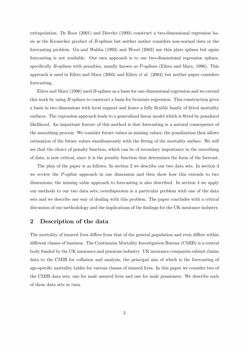
where φi is an age-dependent overdispersion parameter. We use the medians of the rows of

(Z∗ − Z∗)2/Z

∗ as an initial estimate of the φi; medians are preferred to means for robustness

reasons. The left panel of Figure 9 gives a plot of these medians together with their smoothed

values obtained by a one-dimensional P -spline smooth on the log scale; we take these smoothed

values as our estimate of the overdispersion parameters φi in (4.3). One further iteration of (4.3)

gives the right hand panel of Figure 9; the overdispersion has been removed.

The effect of the scaling in both (4.2) and (4.3) is to reduce the exposure from the total

amounts at risk in F to an effective sample size approximated initially by F /A. One consequence

in this “reduction in sample size” is that the resulting fit is considerably stiffer: the degrees of

freedom for the three fits referred to in the preceding paragraphs are 42 (stage 1), 19 and 17

(stage 2).

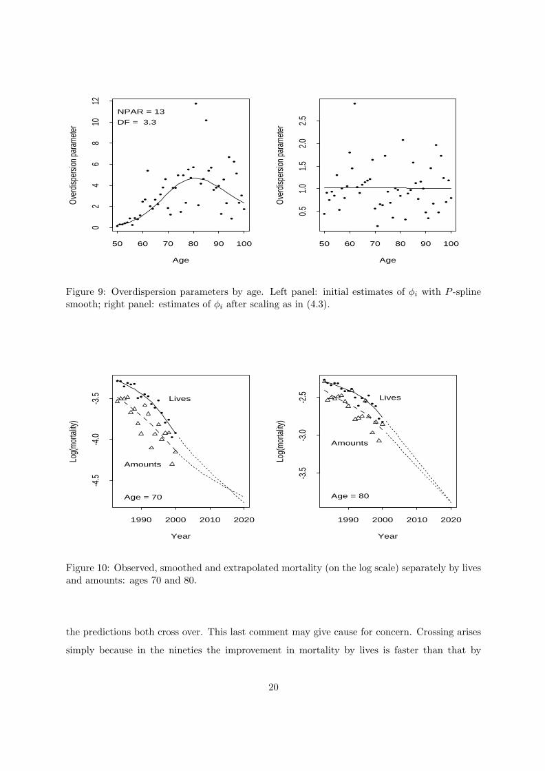
We also used the method of 4.1 to forecast the mortality using the lives data and Figure

10 gives a comparison for two ages of the log(mortality) using the two data sets. We make

three comments: first, the mortality by lives is heavier than by amounts, in line with industry

experience; second, the overdispersion in the amounts data is evident from both plots; third,

19

••••••••••

••

•

•••••••

••

••

•

•

•

•

••

•

•

•

••

•

••

•••

•

•

•

•

•

•

•

••

•

Age

Over

dispe

rsion

par

amet

er

50 60 70 80 90 100

02

46

810

12

NPAR = 13

DF = 3.3

•

••••

•

•

••

•

•

•

•

••••

••

•

•

•

••

•

•

•

•

•••

•

•

••

•

•

•

••

••

•

•

•

•

•

•

•

•

•

Age

Over

dispe

rsion

par

amet

er

50 60 70 80 90 100

0.5

1.0

1.5

2.0

2.5

Figure 9: Overdispersion parameters by age. Left panel: initial estimates of φi with P -splinesmooth; right panel: estimates of φi after scaling as in (4.3).

Year

Log(

mor

tality

)

1990 2000 2010 2020

-4.5

-4.0

-3.5

••••••

••••••

•

•••

••

Age = 70

Lives

Amounts

Year

Log(

mor

tality

)

1990 2000 2010 2020

-3.5

-3.0

-2.5

•••••••••••••

•••

••

Age = 80

Lives

Amounts

Figure 10: Observed, smoothed and extrapolated mortality (on the log scale) separately by livesand amounts: ages 70 and 80.

the predictions both cross over. This last comment may give cause for concern. Crossing arises

simply because in the nineties the improvement in mortality by lives is faster than that by

20

amounts; crossing results. However it is an accepted fact in the industry that mortality by lives

is and will be heavier than that by amounts. This suggests that we build a joint model for

mortality by lives and by amounts, and the regression form of our model makes this particularly

simple. For example, we can fit surfaces with parallel cross sections in age, i.e., we force the

fitted curves in Figure 10 to be parallel. We take lives as the baseline and use ηL = By⊗Baa as

linear predictor. For amounts we add an age dependent constant (the gap between the mortality

curves in Figure 10). If we smooth these gaps then we get ηA = By ⊗Baa+1y ⊗Bag as linear

predictor where 1 is a vector of 1’s, i.e., ηA = ηL + 1y ⊗ Bag. Now we have three smoothing

parameters to choose: the mortality surface (determined by a) is subject to a penalty of the

form (3.17) while the gap (determined by g) is subject to the basic penalty function in (3.3).

The explicit regression formulation is

y =[

yL

yA

], e =

[eL

eA

], B =

[By ⊗ Ba 0By ⊗ Ba 1y ⊗ Ba

], P =

[P 1 00 P 2

](4.4)

where P 1 is given by (3.17) and P 2 by (3.3); the claim numbers and exposures are given by

yL = vec(Y ) and eL = vec(E) and the claim amounts, yA, and amounts at risk, eA, are the

adjusted values defined in (4.3) which gave Figure 10. Figure 11 shows the fitted curves for ages

70 and 80 and both the parallel nature of the curves and the age dependent gaps are evident.

Figure 12 shows the smoothed gaps, Bag, the gaps between the separate smooths for amounts

and lives in Figure 10 averaged over years 1983 to 2000, and the gaps between log(RA) and

log(RL) again averaged over years 1983 to 2000 (ages 50 to 64 are omitted because of missing

values in log(RA) and log(RL)).

We end this section by noting a simple connection between a joint model defined by (4.4)

and the idea of a “standard table”. The insurance industry makes much use of standard tables.

A small number of such tables are used as reference tables and then tables for other classes of

business are given in terms of age adjustments to the standard table. We illustrate the idea with

the lives and amounts model. Suppose we take the lives mortality as the standard. Let ηL be

the fitted linear predictor for lives. Now take ηA = ηL + 1y ⊗ Bag, i.e., ηL is an offset in the

model with data yA and eA, regression matrix B = 1y ⊗ Ba and penalty P = λD′aDa. The

mortality by amounts is then summarized (with reference to the standard table) by Bag where

g is the vector of estimated regression coefficients.

21

Year

Log(

mor

tality

)

1990 2000 2010 2020

-4.5

-4.0

-3.5

••••••

••••••

•

•••

••

Age = 70

Lives

Amounts

Year

Log(

mor

tality

)

1990 2000 2010 2020

-4.0

-3.5

-3.0

-2.5

•••••••••••••

•••

••

Age = 80

Lives

Amounts

Figure 11: Observed, smoothed and extrapolated mortality (on the log scale) by lives andamounts with parallel cross-sections by age: ages 70 and 80.

5 Discussion

We have presented a flexible model for two-dimensional smoothing and shown how it may be

fitted within the framework of a penalized generalized linear model (PGLM). We have concen-

trated on the smoothing of mortality tables for which the Poisson distribution is appropriate,

but the method has much wider application and a number of generalizations. First, the method

can be applied to any GLM with canonical link by replacing the weight matrix W = diag(µ)

by a diagonal matrix with elements w−1ii = (∂ηi/∂µi)2var(yi). Second, the method (which we

applied to data on a regular grid) can be extended to deal with scattered data; see Eilers et al.

(2004). Third, computational issues, which are relatively minor for the data sets considered in

this paper, become a major consideration with larger data sets. An important property of our

model is that there exists an algorithm which reduces both storage requirements and compu-

tational times by an order of magnitude; see again Eilers et al. (2004). Fourth, our method

of forecasting is suitable for the estimation of missing values or the extrapolation of data on

a grid in any direction. All that is required are the regression and penalty matrices, and the

appropriate weight matrix. The extrapolation is then effected by (3.20).

We emphasise the critical role of the order of the penalty, pord. The choice of the order of

the penalty corresponds to a view of the future pattern of mortality: pord = 1, 2 or 3 correspond

22

Age

Gap

50 60 70 80 90 100

-0.4

-0.2

0.0

0.1

0.2

•

•

••

• ••

• •• • •

• •• •

••

••

•

••

•• •

• • ••

•

•

•

••

•

Figure 12: Smoothed gaps (solid line), gaps between separate smooths (dashed line) and datagaps (points).

respectively to future mortality continuing at a constant level, improving at a constant rate or

improving at an accelerating (quadratic) rate. We do not believe pord = 1 is consistent with the

data. A value of pord = 3 has some initial attractions; for example, in the right hand panel of

Figure 6 pord = 3 gives an excellent fit to the “future” data. However, with a fifty year horizon

the quadratic extrapolation gives predictions which seem implausible, and would certainly be

viewed with alarm by the insurance industry.

The failure to predict accurately the fall in mortality rates has had far-reaching consequences

for the UK pensions and annuity business. What comfort can be drawn from the results pre-

sented in this paper? We suggested in our introduction that any such predictions are unlikely to

be correct. The difference between the P -spline and Lee-Carter forecasts identified in section 4.1

only serves to underline the difficulty of forecasting so far ahead. Our estimates of future mortal-

ity come with confidence intervals, and the widths of the confidence intervals indicate the level

of uncertainly associated with the forecast. A prudent course is to allow for this uncertainty by

discounting the predicted rates by a certain amount and our view is that some such discounting

23

procedure is the only reasonable way of allowing for the uncertainty in these, or indeed any,

predictions. The level of discount will have financial implications for the pricing and reserving

of annuities and pensions.

Acknowledgements

We thank the CMIB for providing the data and for providing financial support to all three

authors. We also thank the referees for their careful and constructive comments.

References

Aerts M, Claeskens G, Wand MP (2002) Some theory for penalized spline generalized additive

models. Journal of Statistical Planning and Inference, 103, 455-70.

Brouhns N, Denuit M, Vermunt JK (2002) A Poisson log-bilinear regression approach to the

construction of projected lifetables. Insurance: Mathematics & Economics, 31, 373-93.

Chatfield C (2003) Model selection, data mining and model uncertainty. Proceedings of the 18th

International Workshop on Statistical Modelling, Leuven, Belgium, 79-84.

Clayton D, Schifflers E (1987) Models for temporal variation in cancer rates. II: Age-period-

cohort models. Statistics in Medicine, 6, 469-81.

Cleveland WS, Devlin SJ (1988) Locally weighted regression: an approach to regression analysis

by local fitting. Journal of the American Statistical Association, 83, 597-610.

Coull BA, Ruppert D, Wand MP (2001a) Simple incorporation of interactions into additive

models. Biometrics, 57, 539-45.

Coull BA, Schwartz J, Wand MP (2001b) Respiratory health and air pollution: additive mixed

model analyses. Biostatistics, 2, 337-50.

Currie ID, Durban M (2002) Flexible smoothing with P -splines: a unified approach. Statistical

Modelling, 2, 333-49.

de Boor C (2001) A practical guide to splines. Springer.

Dierckx P (1993) Curve and surface fitting with splines. Oxford: Clarendon Press.

Durban M, Currie ID (2003) A note on P -spline additive models with correlated errors. Com-

putational Statistics, 18, 251-62.

Eilers PHC, Marx BD (1996) Flexible smoothing with B-splines and penalties. Statistical Sci-

ence, 11, 89-121.

Eilers PHC, Marx BD (2002) Generalized linear additive smooth structures. Journal of Com-

24

putational and Graphical Statistics, 11, 758-83.

Eilers PHC, Marx BD (2003) Multivariate calibration with temperature interaction using two-

dimensional penalized signal regression. Chemometrics and Intelligent Laboratory Systems,

66, 159-174.

Eilers PHC, Currie ID, Durban M (2004) Fast and compact smoothing on large multidimensional

grids. Computational Statistics and Data Analysis, to appear.

Gu C, Wahba G (1993) Semiparametric analysis of variance with tensor product thin plate

splines. Journal of the Royal Statistical Society, Series B, 55, 353-368.

Hastie TJ, Tibshirani RJ (1990) Generalized additive models. London: Chapman & Hall.

Hurvich CM, Simonoff JS, Tsai C-L (1998) Smoothing parameter selection in nonparametric

regression using an improved Akaike information criterion. Journal of the Royal Statistical

Society, Series B, 60, 271-294.

Lee TCM (2003) Smoothing parameter selection for smoothing splines: a simulation study.

Computational Statistics & Data Analysis, 42, 139-148.

Lee RD, Carter LR (1992) Modeling and forecasting U.S. mortality. Journal of the American

Statistical Association, 87, 659-75.

Lin X, Zhang D (1999) Inference in generalized additive mixed models by using smoothing

splines. Journal of the Royal Statistical Society, Series B, 61, 381-400.

Marx BD, Eilers PHC (1998) Direct generalized additive modeling with penalized likelihood.

Computational Statistics & Data Analysis, 28, 193-209.

Marx BD, Eilers PHC (1999) Generalized linear regression on sampled signals and curves: a

P -spline approach. Technometrics, 41, 1-13.

Parise H, Wand MP, Ruppert D, Ryan L (2001) Incorporation of historical controls using semi-

parametric mixed models. Journal of the Royal Statistical Society, Series C, 50, 31-42.

Ruppert D (2002) Selecting the number of knots for penalized splines. Journal of Computational

and Graphical Statistics, 11, 735-57.

Ruppert D, Carroll RJ (2000) Spatially-adaptive penalties for spline fitting. Australian and New

Zealand Journal of Statistics, 42, 205-24.

Searle SR (1982) Matrix algebra useful for statistics. New York: John Wiley & Sons.

Schwarz G (1978) Estimating the dimension of a model. Annals of Statistics, 6, 461-64.

Wand MP (1999) On the optimal amount of smoothing in penalised spline regression. Biometrika,

86, 936-40.

Wand MP (2003) Smoothing and mixed models. Computational Statistics, 18, 223-50.

25

Wood SN (2003) Thin plate regression splines. Journal of the Royal Statistical Society, Series

B, 65, 95-114.

Wood SN, Augustin NH (2002) GAMs with integrated model selection using penalized regression

splines and applications to environmental modelling. Ecological Modelling, 157, 157-77.

26