Full Terms & Conditions of access and use can be found athttps://www.tandfonline.com/action/journalInformation?journalCode=glma20

Linear and Multilinear Algebra

ISSN: 0308-1087 (Print) 1563-5139 (Online) Journal homepage: https://www.tandfonline.com/loi/glma20

Geometric mean of partial positive definitematrices with missing entries

Hayoung Choi, Sejong Kim & Yuanming Shi

To cite this article: Hayoung Choi, Sejong Kim & Yuanming Shi (2019): Geometric meanof partial positive definite matrices with missing entries, Linear and Multilinear Algebra, DOI:10.1080/03081087.2019.1585741

To link to this article: https://doi.org/10.1080/03081087.2019.1585741

Published online: 01 Mar 2019.

Submit your article to this journal

Article views: 7

View Crossmark data

LINEAR ANDMULTILINEAR ALGEBRAhttps://doi.org/10.1080/03081087.2019.1585741

Geometric mean of partial positive definite matrices withmissing entries

Hayoung Choia, Sejong Kimb and Yuanming Shia

aSchool of Information Science and Technology, Shanghai Tech University, Shanghai, People’s Republic ofChina; bDepartment of Mathematics, Chungbuk National University, Cheongju, Republic of Korea

ABSTRACTIn this paper the geometric mean of partial positive definite matriceswith missing entries is considered. The weighted geometric mean oftwo sets of positive matrices is defined, and we show whether sucha geometric mean holds certain properties which the weighted geo-metric mean of two positive definite matrices satisfies. Additionally,counterexamples demonstrate that certain properties do not hold.A Loewner order on partial Hermitian matrices is also defined. Theknown results for the maximum determinant positive completionare developed with an integral representation, and the results areapplied to the weighted geometric mean of two partial positive defi-nite matrices with missing entries. Moreover, a relationship betweentwo positive definite completions is established with respect to theirdeterminants, showing relationshipbetween their entropy for a zero-mean,multivariate Gaussian distribution. Computational results aswell as one application are shown.

ARTICLE HISTORYReceived 11 January 2018Accepted 14 February 2019

COMMUNICATED BYY. Lim

KEYWORDSGeometric mean; positivedefinite completions;maximum determinant;entropy; covariance matrix

1. Introduction

The geometric mean of two positive definite matrices A and B is given by an explicitformula [1,2]:

A#1/2B = A1/2(A−1/2BA−1/2)1/2A1/2. (1)

This is known as the unique positive definite solution X of the Riccati equation XA−1X =B [3,4]. Moreover, it can be extended to the unique geodesic t ∈ [0, 1] �→ A#tB =A1/2(A−1/2BA−1/2)tA1/2 connecting fromA to B for the Riemannian trace distance on theopen convex cone of positive definite matrices [5,6]. This geodesic is called the weightedgeometric mean of A and B. A various theories of extending two-variable geometric meanto multi-variable case have been developed: see [7–11]. A general framework of multi-variable operator means containing the multivariable geometric mean as a special caseis considered [12]. Multi-variable geometric means as well as the two-variable geomet-ric mean of positive definite matrices have been considered as important objects in manypure and applied areas, such as data points in a diverse area of settings [13–15].

CONTACT Sejong Kim skim@chungbuk.ac.kr

© 2019 Informa UK Limited, trading as Taylor & Francis Group

2 H. CHOI ET AL.

In many research, there is the potential for missing or incomplete data since dataobtained from physical experiments and phenomena are often corrupt or incomplete. Theissue with missing data is that nearly all classic and modern statistical and analytical tech-niques deal with complete data. It is vital to be able to deal with missing data rather than todelete the incomplete data from the analysis. Over the past 20 years techniques for dealingwithmissing data in themost appropriate and desirable way possible have been extensivelystudied inmany different fields such as data analysis, statistics, optimization, matrix theory[16–19].

Covariance matrices are used as features for many signal and image processing appli-cations, including biomedical image segmentation, radar detection, texture analysis, etc.Recently new geometric approach has been developed for various problems, such as howto measure the distance between two covariance matrices, how to find the average matrixof covariance matrices [20–28]. Especially, in [29] Riemannian mean of covariance matri-ces to space-time adaptive processing is considered. Recently it becomes more and moreimportant to deal with incomplete covariance matrices in perturbed environment [30].General strategy for completing a partially specified covariance matrix was studied byDempster [31]. A zero-mean, multivariate Gaussian distribution on Rn with density

f (x) = (2π)−n/2|�|−1/2 exp{−12x��−1x

}is considered with a partially specified covariance matrix �. Dempster proposed a com-pletion which maximizes the entropy

H(f ) = −∫

Rnlog(f (x))f (x)dx (2)

= 12log(det�) + 1

2n(1 + log (2π)), (3)

implying that the completion has the maximum determinant. For more information aboutthe maximum determinant and the maximum entropy [32–34].

We consider the geodesic and the geometric mean of two covariance matrices asspace-time adaptive processing, additionally with missing entries, i.e. partially specifiedcovariance matrices. As the process of averaging, the concept of geometric mean of twopositive definite matrices with missing entries will play a role to apply a geometric meanto applications in such areas. In this paper we mainly study the geometric mean of twopartial positive definite matrices with missing entries. After a series of preliminary defini-tions and known results for a graph, a partial matrix, and the weighted geometric mean oftwo positive matrices in Section 2 that will be used throughout this paper, we consider inSection 3 the weighted geometric mean of two subsets of the positive cone. Several mean-ingful examples for the geometricmean of two subsets are given, and topological propertiesfor it are shown. Using the geometric mean of two sets of positive definite completions,in Section 4 we define the geometric mean of two partial positive definite matrices andshow that it holds several of the known properties for the geometric mean of two positivedefinite matrices. In Section 5, we define a partial Loewner order for partial Hermitianmatrices and characterize the difference of two partial matrices. In Section 6, the knownresults for a positive definite completion of maximizing determinant are developed with

LINEAR ANDMULTILINEAR ALGEBRA 3

an integral representation and are applied to the weighted geometric mean of two partialpositive definite matrices. Some interesting computational results are found in Section 7.

2. Preliminary

2.1. Graph and positivematrix completion

In 1981, H. Dym and I. Gohberg studied extensions of band matrices with band inverses[35]. In 1984, R. Grone, C. R. Johnson, E. M. Sá, and H. Wolkowicz considered positivedefinite completion of partial Hermitian matrices (some entries specified, some missing)[36]. They showed that if the undirected graph of the specified entries is chordal, a positivedefinite completion necessarily exists. Johnson, Lundquist, and Naevdal studied positivedefinite Toeplitz matrix completions in 1997. In [37], they proved that a pattern P of an(n + 1) × (n + 1) partial Toeplitzmatrix is positive (semi) definite completable if and onlyif P = {k, 2k, . . . ,mk} for somem ∈ N and k ∈ N.

LetV be the set of vertices, and let {x, y} denote the edge connecting two points x, y ∈ V .A finite undirected graph is a pair G = (V ,E) where the set V of vertices is finite, and theset E of edges is a subset of the set {{x, y} : x, y ∈ V}. In general Emay contain loops whichmeans that x= y. In this paper we assume that the graph always has all loops. Without lossof generality we assume that V = {1, 2, . . . , n}.

Define a G-partial matrix as a set of complex numbers, denoted by [aij]G or A(G),where aij is specified if and only if {i, j} ∈ E. A completion of A(G) = [aij]G is an n × nmatrix M = [mij] which satisfies mij = aij for all {i, j} ∈ E. We say that M is a positive(semi-)definite completion of A(G) if and only if M is a completion of A(G) and M ispositive (semi-)definite. A clique is a subset C ⊂ V having the property that {x, y} ∈ Efor all x, y ∈ C. A cycle in G is a sequence of pairwise distinct vertices γ = (v1, . . . , vs)having the property that {v1, v2}, {v2, v3}, . . . , {vs−1, vs}, {vs, v1} ∈ E, and s is referred to asthe length of the cycle. A chord of the cycle γ is an edge {vi, vj} ∈ E where 1 ≤ i < j ≤ s,{vi, vj} �= {v1, vs}, and |i − j| ≥ 2.

Assume V = {1, . . . , n}, and let A(G) = [aij]G be a G-partial matrix. We say that A(G)

is a partial positive (semi-)definite if

aji = aij for all {i, j} ∈ E

and for any clique C of G, this principal submatrix [aij]i,j∈C of A(G) is positive (semi-)definite. The graph G is called positive (semi-)definite completable if any G-partial positive(semi-)definite matrix has a positive (semi-)definite completion.

The following proposition shows that the terms ‘positive definite completable ’ and‘positive semi-definite completable’ coincide [36].

Proposition 2.1: A graph G is positive definite completable if and only if G is positive semi-definite completable.

From now on, we will henceforth only use the term ‘completable’. A graph G is chordalif there are no minimal cycles of length ≥ 4. Equivalently, every cycle of length ≥ 4 has achord. This concept characterizes completable graphs [36].

4 H. CHOI ET AL.

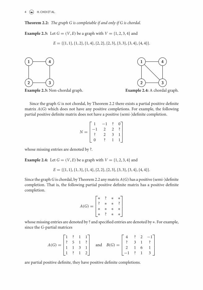
Theorem 2.2: The graph G is completable if and only if G is chordal.

Example 2.3: Let G = (V ,E) be a graph with V = {1, 2, 3, 4} and

E = {{1, 1}, {1, 2}, {1, 4}, {2, 2}, {2, 3}, {3, 3}, {3, 4}, {4, 4}}.

Example 2.3: Non-chordal graph. Example 2.4: A chordal graph.

Since the graph G is not chordal, by Theorem 2.2 there exists a partial positive definitematrix A(G) which does not have any positive completions. For example, the followingpartial positive definite matrix does not have a positive (semi-)definite completion.

N =

⎡⎢⎢⎣1 −1 ? 0

−1 2 2 ?? 2 3 10 ? 1 1

⎤⎥⎥⎦whose missing entries are denoted by ?.

Example 2.4: Let G = (V ,E) be a graph with V = {1, 2, 3, 4} and

E = {{1, 1}, {1, 3}, {1, 4}, {2, 2}, {2, 3}, {3, 3}, {3, 4}, {4, 4}}.

Since the graphG is chordal, by Theorem 2.2 anymatrixA(G) has a positive (semi-)definitecompletion. That is, the following partial positive definite matrix has a positive definitecompletion.

A(G) =

⎡⎢⎢⎣∗ ? ∗ ∗? ∗ ∗ ?∗ ∗ ∗ ∗∗ ? ∗ ∗

⎤⎥⎥⎦whosemissing entries are denoted by ? and specified entries are denoted by ∗. For example,since the G-partial matrices

A(G) =

⎡⎢⎢⎣1 ? 1 1? 5 1 ?1 1 3 11 ? 1 2

⎤⎥⎥⎦ and B(G) =

⎡⎢⎢⎣4 ? 2 −1? 3 1 ?2 1 6 1

−1 ? 1 3

⎤⎥⎥⎦are partial positive definite, they have positive definite completions.

LINEAR ANDMULTILINEAR ALGEBRA 5

Let Mm×n := Mm×n(C) be a set of all m × n matrices with entries in the field C ofcomplex numbers. We equip onMm×n with the inner product defined as

〈A,B〉 := tr(A∗B) =m,n∑i,j=1

aijbij,

for A = [aij],B = [bij] ∈ Mm×n, where A∗ = AT is a complex conjugate transpose of A.The inner product naturally gives us an l2 norm, known as the Frobenius norm andHilbert–Schmidt norm, defined by

‖A‖2 = [tr(A∗A)]1/2.

We simply denote asMn := Mn×n. We also denote as GLn the general linear group inMn.

Remark 2.5: The operator norm of A ∈ Mn is defined as

‖A‖ := max‖x‖2=1

‖Ax‖2.

Note that

‖A‖2 =[ n∑i=1

σ 2i (A)

]1/2and ‖A‖ = σ1(A),

where σ1(A) ≥ · · · ≥ σn(A) are (non-negative) singular values of A in decreasing order.Since ‖A‖ ≤ ‖A‖2 ≤ n‖A‖2, two norms ‖ · ‖2 and ‖ · ‖ are compatible.

Let H ⊂ Mn be the real vector space of all Hermitian matrices, and let P ⊂ H be theopen convex cone of n × n positive definite matrices. Then the closure P of P consists ofall n × n positive semi-definite matrices. For any A,B ∈ H we denote as A ≤ B if and onlyif B − A ∈ P, and A<B if and only if B − A ∈ P. This is known as the Loewner partialordering [38, Section 7.7].

The Frobenius norm ‖ · ‖2 gives rise to the Riemannian trace metric on P given by

δ(A,B) = ‖ log(A−1/2BA−1/2)‖2 (4)

for any A,B ∈ P. Then P is a Cartan–Hadamard manifold, a simply connected completeRiemannian manifold with non-positive sectional curvature. The curve

[0, 1] � t �→ A#tB := A1/2(A−1/2BA−1/2)tA1/2

is the unique geodesic from A to B, called the weighted geometric mean of positive definitematrices A and B. Note that A#B := A#1/2B is the unique midpoint between A and B forthe Riemannian metric. We review several known properties of the weighted geometricmean on the open convex cone P of positive definite matrices.

Theorem 2.6: The weighted two-variable geometric mean satisfies the following: for any A,B, C, D ∈ P and t ∈ [0, 1]

(1) A#tB = A1−tBt if A and B commute.

6 H. CHOI ET AL.

(2) (aA)#t(bB) = a1−tbt(A#tB) for any a,b>0.(3) A#tB = B#1−tA.(4) A#tB ≤ C#tD whenever A ≤ C and B ≤ D.(5) [0, 1] × P × P � (t,A,B) �→ A#tB ∈ P is continuous.(6) S∗(A#tB)S = (S∗AS)#t(S∗BS) for any invertible S ∈ GLn.(7) [(1 − λ)A + λB]#t[(1 − λ)C + λD] ≥ (1 − λ)(A#tC) + λ(B#tD) for any λ ∈ [0, 1].(8) (A#tB)−1 = A−1#tB−1.(9) det(A#tB) = (detA)1−t(detB)t .(10) [(1 − t)A−1 + tB−1]−1 ≤ A#tB ≤ (1 − t)A + tB for any t ∈ [0, 1].

Remark 2.7: Item (5) can be described as themap [0, 1] × P × P � (t,A,B) �→ A#tB ∈ P

is continuous with respect to the Riemannian trace metric δ:

δ(A#sB,C#tD) ≤ δ(A#sB,A#tB) + δ(A#tB,C#tD)

≤ |s − t|δ(A,B) + (1 − t)δ(A,C) + tδ(B,D)

for any A,B,C,D ∈ P and s, t ∈ [0, 1].

Remark 2.8: One can define the weighted geometric mean for positive semi-definitematrices A and B such as

A#tB := limε→0+

(A + εI)#t(B + εI). (5)

By Theorem 2.6 (4), (A + εI)#t(B + εI) is monotone decreasing on ε > 0 and is boundedbelow by O. So it converges, and thus, the equation (5) is well-defined.

3. Weighted geometric mean of two subsets of the positive cone

In this paper we deal with the following weighted geometric mean of two subsets of P andsee its geometric properties.

Definition 3.1: Let S ⊂ P and T ⊂ P, and let t ∈ [0, 1]. The weighted geometric meanof two subsets of positive definite matrices is defined by

S#tT := {S#tT | S ∈ S , T ∈ T }.Example 3.2: The weighted geometric mean of two subsets of P has a very importantconcept in the theory of operator, matrix means, and approximation. In order to see thisinsight, we give several examples in the following.

(1) The weighted geometric mean A#tB of A and B in P is a special example of that oftwo subsets S = {A} ⊂ P and T = {B} ⊂ P. Moreover, if two subsets S and T havecardinalities of p and q, respectively, then the cardinality of S#tT is less than or equalto pq.

(2) For givenA,B ∈ P, considerS = {A + εI : ε1 > 0} and T = {B + ε2I : ε > 0}. ThenS ,T ⊂ P, and

(A + ε1I)#t(B + ε2I) ∈ S#tT ,

which is a generalized form of the right-hand side in the limit of (5).

LINEAR ANDMULTILINEAR ALGEBRA 7

(3) For A,B,C,D ∈ P let S = [A,B] = {X ∈ P : A ≤ X ≤ B} and T = [C,D] = {Y ∈P : C ≤ Y ≤ D}. Then by monotonicity of the geometric mean in Theorem 2.6 (4),

S#tT ⊆ [A#tC,B#tD].

(4) For A,B ∈ P let S = {X ∈ H : ‖A − X‖ ≤ r1} and T = {Y ∈ H : ‖B − Y‖ ≤ r2}.Then S ,T ⊂ P for sufficiently small r1, r2 > 0. So the weighted geometric mean ofS and T , S#tT , can be considered as a set of approximations of A#tB.

Especially, for the case of (3) in Example 3.2 the following property which is similar to[4, Theorem 3.4] holds.

Proposition 3.3: Assume that two subsets S and T of P are totally ordered with respect toLoewner order. Then

M#N = max{X ∈ H :

(A XX B

)≥ 0,A ∈ S ,B ∈ T

}, (6)

where M is the maximum element of S and N is the maximum element of T .

Proof: It is known from Theorem 4.1.3 (iii) in [5] that for given A ∈ S ,B ∈ T

A#B = max{X ∈ H :

(A XX B

)≥ 0}.

Since two subsets S and T of P are totally ordered with respect to Loewner order, A ≤M for all A ∈ S and B ≤ N for all B ∈ T . By the monotonicity of geometric mean inTheorem 2.6 (4), A#B ≤ M#N, and hence, we obtain (6). �

Theorem 3.4: Let S ,T ⊂ P, and let t ∈ [0, 1]. Then

(1) if S and T are bounded, then so is S#tT ,(2) if S and T are closed, then so is S#tT .

Hence, S#tT is compact whenever S ,T are compact.

Proof: Note that it is enough to show (1) and (2) for compactness, since P is a subset ofEuclidean space H.

(1) Assume that S and T are bounded. By Remark 2.5 ‖A‖ ≤ c for all A ∈ S and someconstant c>0, and ‖B‖ ≤ d for all B ∈ T and some constant d>0. Then 0 < A ≤ cIfor all A ∈ S , and 0 < B ≤ dI for all B ∈ T . By Example 3.2 (3), and Theorem 2.6 (1)and (4), it follows that

0 < A#tB ≤ c1−tdtI.

That is, ‖A#tB‖ ≤ c1−tdt , and thus, S#tT is bounded.

8 H. CHOI ET AL.

(2) LetS and T be closed. Assume that sequencesAn ∈ S and Bn ∈ S converge toA ∈ Sand B ∈ T with respect to the Riemannian distance, respectively. By continuity of thegeometric mean in Theorem 2.6 (5) and Remark 2.7,

An#tBn → A#tB ∈ S#tT .

Thus, S#tT is closed.

�

Remark 3.5: Note that the union of a finite number of compact subsets of P is compactand the intersection of any family of compact subspace of P is compact. If {Si} and {Tj} arecollections of compact subsets of P, then( n⋃

k=1

Sik

)#

( m⋃k=1

Tjk

)and

(⋂iSi

)#

⎛⎝⋂jTj

⎞⎠are compact.

Remark 3.6: Assume that S ,T ⊂ P are convex. Let A,B ∈ S and C,D ∈ T . Since S andT are convex, (1 − λ)A + λB ∈ S and (1 − λ)C + λD ∈ T for any λ ∈ [0, 1], and hence,[(1 − λ)A + λB]#t[(1 − λ)C + λD] ∈ S#tT . On the other hand, it holds from the jointconcavity of geometric mean in Theorem 2.6 (7) that

[(1 − λ)A + λB]#t[(1 − λ)C + λD] ≥ (1 − λ)(A#tC) + λ(B#tD)

for any λ ∈ [0, 1]. It is questionable whether or not (1 − λ)(A#tC) + λ(B#tD) ∈ S#tT . Ifit is true, then we can say that S#tT is convex.

4. Geometric mean of partial positive matrices

From now on, we consider the geometric mean of partial positive matrices. In this paper,we assume that any graph G always includes all loops. That is, any partial matrix doesnot have missing entries on diagonal. Recall that H ⊂ Mn is the real vector space of allHermitian matrices, P ⊂ H is the open convex cone of n × n positive definite matrices,and the closure P of P consists of all n × n positive semi-definite matrices. We define

H(G) := {A(G) : A(G) is a n × nG-partial Hermitian matrix.},P(G) := {A(G) ∈ H(G) : A(G) is a partial positive definite matrix.}.

For a given G-partial matrix A(G), we denote as p[A(G)] and p+[A(G)] the sets of allpositive semi-definite and positive definite completions of A(G), respectively.

Theorem 4.1: Let A(G) be a partial positive semidefinite matrix with a completable graphG. Then p[A(G)] is non-empty, convex, and compact.

LINEAR ANDMULTILINEAR ALGEBRA 9

Proof: Since G is a positive completable graph and A(G) is a partial positive semi-definitematrix, clearly p[A(G)] is non-empty. IfM,N ∈ p[A(G)], then (1 − t)M + tN ∈ p[A(G)]for t ∈ [0, 1], so p[A(G)] is convex. Since we assume that diagonal entries are given,p[A(G)] is bounded, since

‖M‖2 =[ n∑i=1

λ2i (M)

]1/2≤ tr(M) =

n∑i=1

mii < ∞

for anyM ∈ p[A(G)], where λi(M) denotes the non-negative eigenvalue ofM.Nowwe show thatp[A(G)] is closed. LetMk = [m(k)

ij ] be a sequence inp[A(G)] converg-ing toM = [mij] in the Frobenius norm. SinceMk ∈ P for all k, we haveM ∈ P. Moreover,since

|m(k)ij − mij| ≤ ‖Mk − M‖2,

we have thatm(k)ij → mij as k → ∞ for all 1 ≤ i, j ≤ n. Sincem(k)

ij = mij for all k and {i, j} ∈E, taking the limit as k → ∞ yields thatmij = aij for all {i, j} ∈ E. So,M is a positive semi-definite completion of A(G), that is,M ∈ p[A(G)]. �

Remark 4.2: For a partial positive definite matrix A(G) with a completable graph G,one can see easily that p+[A(G)] ∈ P(G) is non-empty, convex, and bounded. Sincep+[A(G)] ⊂ p[A(G)], we have p+[A(G)] ⊂ p[A(G)] = p[A(G)] by Theorem 4.1, wherep+[A(G)] is the closure of p+[A(G)]. On the other hand, it is questionable that p[A(G)] ⊂p+[A(G)].

Let G and F be given completable graphs. One can naturally ask to define the geometricmean of partial positive definite matrices A(G) and B(F). Using the geometric mean ofsubsets of P in Definition 3.1, we define the geometric mean of two partial positive definitematrices A(G) and B(F) as

A(G)#tB(F) := p+[A(G)]#tp+[B(F)], (7)

where t ∈ [0, 1].

Remark 4.3: Using Remark 2.8, one can define the geometric mean of partial positivesemi-definite matrices A(G) and B(F) as

p[A(G)]#tp[B(F)].

There are some results for the geometric mean of positive semi-definite matrices [3], butit holds more limited properties than that of positive definite matrices. So we consider inthis article the geometric mean of partial positive definite matrices.

Remark 4.4: By Theorem 3.4 and Reamrk 4.2, A(G)#tB(F) is bounded for partial positivedefinite matrices A(G) and B(F) with completable graphs G and F.

It would be interesting to find some properties for A(G)#tB(F) corresponding to thosein Theorem 2.6.

10 H. CHOI ET AL.

Remark 4.5: Note thatA(G)#tA(G) �= p+[A(G)], sinceA1#tA2 may not be a positive def-inite completion of A(G) even though A1,A2 ∈ p+[A(G)]. For instance, see Example 2.4.Let

A1 =

⎡⎢⎢⎣1 1 1 11 5 1 11 1 3 11 1 1 2

⎤⎥⎥⎦ , A2 =

⎡⎢⎢⎣1 −1 1 1

−1 5 1 −11 1 3 11 −1 1 2

⎤⎥⎥⎦ .

Then A1 and A2 are positive definite completions of A(G). However,

A1#A2 ≈

⎡⎢⎢⎣0.8750 −0.0769 1 0.8750

−0.0769 4.1251 1 −0.07691 1 3 1

0.8750 −0.0769 1 1.8750

⎤⎥⎥⎦ ,

which is not a positive definite completion of A(G). Clearly, it holds that p+[A(G)] ⊂A(G)#A(G).

For A(G),B(G) ∈ H(G) with a given graph G, the sum of two G-partial matrices and thescalar product of a G-partial matrix, denoted by A(G) + B(G) and αA(G) are defined by

[A(G) + B(G)]ij ={aij + bij if {i, j} ∈ E,missing otherwise,

[αA(G)]ij ={

αaij if {i, j} ∈ E,missing otherwise,

where A(G) = [aij]{i,j}∈E and B(G) = [bij]{i,j}∈E, respectively.Note that A(G) + B(G) and αA(G) are in H(G). It is natural to define the difference of

two G-partial matrices as A(G) − B(G) := A(G) + (−1)B(G).Let S ⊂ P and let α > 0. For convenience, we denote

αS : = {αA : A ∈ S},S−1 : = {A−1 : A ∈ S}.

Note that αS ,S−1 ⊂ P. It is trivial that

αp+[A(G)] = p+[αA(G)], p+[A(G) + B(G)] = p+[A(G)] + p+[B(G)].

Proposition 4.6: For completable graphs G and F, let A(G) and B(F) be partial positivedefinite matrices. Then the following hold:

(1) a1−tbt(p+[A(G)]#tp+[B(F)]) = (ap+[A(G)])#t(bp+[B(F)]) for any a,b>0,(2) p+[A(G)]#tp+[B(F)] = p+[B(F)]#1−tp

+[A(G)], and(3) (p+[A(G)]#tp+[B(F)])−1 = p+[A(G)]−1#tp+[B(F)]−1.

LINEAR ANDMULTILINEAR ALGEBRA 11

Proof: Let A(G) ∈ P(G) and B(F) ∈ P(F).

(1) Let A#tB ∈ p+[A(G)]#tp+[B(F)], where A ∈ p+[A(G)] and B ∈ p+[B(F)]. ThenaA ∈ ap+[A(G)] = p+[aA(G)], and bB ∈ p+[bB(G)]. By Theorem 2.6 (2),

a1−tbt(A#tB) = (aA)#t(bB) ∈ (ap+[A(G)])#t(bp+[B(F)]).

So a1−tbt(p+[A(G)]#tp+[B(F)]) ⊆ (ap+[A(G)])#t(bp+[B(F)]).Let C#tD ∈ (ap+[A(G)])#t(bp+[B(F)]), where C ∈ p+[aA(G)] and D ∈ p+[bB(F)].Then a−1C ∈ p+[A(G)] and b−1D ∈ p+[B(F)], and furthermore, by Theorem 2.6 (2)

C#tD = a1−tbt[(a−1C)#t(b−1D)] ∈ a1−tbt(p+[A(G)]#tp+[B(F)]

).

(2) By Theorem 2.6 (3), A#tB = B#1−tA for any A ∈ p+[A(G)] and B ∈ p+[B(F)]. Thus,it is proved.

(3) By Theorem 2.6 (8), (A#tB)−1 = A−1#tB−1 for anyA ∈ p+[A(G)] and B ∈ p+[B(F)].Thus, it is proved.

�

5. Difference of partial matrices and Loewner order on partial matrices

Analogous to the Loewner order on H, we define the relation for G-partial semi-definitematrices.

Definition 5.1: For a given completable graph G, we define the relation ≤ on H(G) asfollows:

(i) A(G) ≥ B(G) if and only if A(G) − B(G) ∈ P(G);(ii) A(G) > B(G) if and only if A(G) − B(G) ∈ P(G).

Theorem5.2: The relation ≤ is indeed a partial order onH(G)with a completable graphG.

Proof: Let G be a completable graph.(Reflexive) Since A(G) − A(G) is the zero matrix, it holds A(G) ≤ A(G) for all A(G) ∈

H(G).(Anti-symmetric) Suppose that A(G) ≤ B(G) and B(G) ≤ A(G) for A(G),B(G) ∈

H(G). Since A(G) − B(G) and A(G) − B(G) partial positive semidefinite, then the diag-onal entries of A(G) − B(G) must be 0, implying A(G) − B(G) = 0. Thus A(G) = B(G).

(Transitive) Suppose that A(G) ≤ B(G) and B(G) ≤ C(G) for A(G),B(G),C(G) ∈H(G). Let α ⊂ {1, 2, . . . , n} such that A(G)[α] be a fully specified principal submatrix.Clearly, M = (A(G) − B(G))[α] and N = (B(G) − C(G))[α] are fully specified princi-pal submatrices of A(G) − B(G) and B(G) − C(G), respectively. Since A(G) − B(G) andB(G) − C(G) are partial positive semidefinite,M andN are positive semidefinite. Note thatM+N is a fully specified principal submatrix of A(G) − C(G) and positive semidefinite.Since α is arbitrary, every fully specified submarix ofA(G) − C(G) is positive semidefinite,implying A(G) ≤ C(G). �

12 H. CHOI ET AL.

Example 5.3: Consider the following G-partial (positive) matrices:

A(G) =

⎡⎢⎢⎣3 ? 2 1? 6 1 ?2 1 4 11 ? 1 5

⎤⎥⎥⎦ , B(G) =

⎡⎢⎢⎣1 ? 1 1? 5 1 ?1 1 3 11 ? 1 2

⎤⎥⎥⎦ .

Since the difference

C(G) := A(G) − B(G) =

⎡⎢⎢⎣2 ? 1 0? 1 0 ?1 0 1 00 ? 0 3

⎤⎥⎥⎦is partial positive definite, by the definition A(G) > B(G).

Remark 5.4: In general, the existence of positive completions of two partial matricesA(G)

and B(G) does not guarantee the existence of positive completion of A(G) − B(G). Forexample, the partial matricesA(G) and B(G) in Example 5.3 have positive definite comple-tions (see Example 2.4). Since the difference C(G) is partial positive definite with positivecompletable graph G, it also has positive definite completions. On the other hand, the par-tial matrix A(G) − 3B(G) does not have any positive (semi-)definite completion since it isnot partial positive (semi-)definite although A(G) ≥ 0, 3B(G) ≥ 0, and they have positive(semi-)definite completions.

Lemma 5.5: Let G be a given completable graph. Suppose that A(G) and B(G) are partialpositive definite matrices. Then p+[A(G) − B(G)] ⊂ p+[A(G)] − p+[B(G)].

Proof: LetG = (V ,E) be a given completable graph. If p+[A(G) − B(G)] = ∅, it is trivial.Let C ∈ p+[A(G) − B(G)]. Then C is a positive definite completion of A(G) − B(G). Thatis, there exist a positive definite matrix C = [cij] such that cij = aij − bij for all {i, j} ∈ E,where A(G) = [aij]{i,j}∈E and B(G) = [bij]{i,j}∈E. Let B = [bij] ∈ p+[B(G)]. Since B>0and C>0, we have B+C>0. Since bij + cij = aij for all {i, j} ∈ E, it follows that B + C ∈p+[A(G)]. Since B is arbitrary, it holds that B + C ∈ p+[A(G)] for all B ∈ p+[B(G)]. Thus,C = (B + C) − B ∈ p+[A(G)] − p+[B(G)]. �

Remark 5.6: (i) For a completable graphG, assume thatA(G) and B(G) are partial posi-tive semi-definitematrices. Then p[A(G) − B(G)] ⊂ p[A(G)] − p[B(G)] by followingthe proof of Lemma 5.5 similarly to positive semi-definite completions.

(ii) Since p+[A(G)] − p+[B(G)] may or may not include an element which is not apositive definite matrix, in general, p+[A(G) − B(G)] �= p+[A(G)] − p+[B(G)]. Forexample, consider the following partial positive definite matrices.

A(G) =⎡⎣2.5 1 ?

1 2.5 1? 1 2.5

⎤⎦ , B(G) =⎡⎣2 1 ?1 2 1? 1 2

⎤⎦ .

LINEAR ANDMULTILINEAR ALGEBRA 13

Then it is clear that

A =⎡⎣2.5 1 1

1 2.5 11 1 2.5

⎤⎦ ∈ p[A(G)], B =⎡⎣2 1 01 2 10 1 2

⎤⎦ ∈ p[B(G)],

and

A − B =⎡⎣0.5 0 1

0 0.5 01 0 0.5

⎤⎦ ∈ p+[A(G)] − p+[B(G)].

However, A − B /∈ p+[A(G) − B(G)] since A−B is not positive definite. This showsthat A(G) < B(G) does not imply A<B for all A ∈ p+[A(G)] and B ∈ p+[B(G)].

Theorem5.7: LetGbe a given completable graph. Suppose thatA(G) andB(G) areG-partialmatrices with 0 < B(G) < A(G). Then

p+[A(G) − B(G))] = (p+[A(G)] − p+[B(G)]) ∩ P.

That is, all positive completions of A(G) − B(G) are expressed as differences of positivecompletions of A(G) and B(G).

Proof: Let C ∈ p+[A(G) − B(G)]. Then by Lemma 5.5 it follows that C ∈ p+[A(G)] −p+[B(G)]. Since C is positive definite, it follows that C ∈ (p+[A(G)] − p+[B(G)]) ∩ P,so p+[A(G) − B(G)] ⊂ (p+[A(G)] − p+[B(G)]) ∩ P. LetD ∈ (p+[A(G)] − p+[B(G)]) ∩P. Then there exist M ∈ p+[A(G)] and N ∈ p+[B(G)] such that D=M−N is positivedefinite. SinceM − N ∈ p+[A(G) − B(G)], we have that D ∈ p+[A(G) − B(G)]. �

6. Maximizing the determinant

For a given completable graphG, we see in this section several interesting consequences forpositive definite completions of G-partial positive matrices maximizing the determinantwith the previous notions of geometric mean and order relation.

Lemma 6.1: [36, Lemma 1] The function f (A) = log det (A) is strictly concave onp+[A(G)].

Theorem 6.2: Let G be a given completable graph, and let A(G) be a G-partial matrix withA(G) > 0. Then there exists a unique positive definite completion of A(G), say A, such that

det(A) = max {det(M) : M ∈ p+[A(G)]}.

Furthermore, A is the unique positive definite completion of A(G) whose inverse C = [cij]satisfies

cij = 0 for all {i, j} /∈ E.

Proof: It follows by Lemma 6.1 amd Theorem 4.1 (see [36]). �

14 H. CHOI ET AL.

Now we investigate relationship between A and other positive definite completions fortheir determinants.

Theorem 6.3: Let G be a given completable graph, and let A(G) be a G-partial matrix withA(G) > 0. For 0 < k < det(A), there exists A ∈ p+[A(G)] such that det(A) = k.

Proof: Since p[A(G)] is convex, it is also path-connected, hence connected. Since thedeterminant, det : p[A(G)] → R, is a continuous function on p[A(G)], the range of thedeterminant function is connected. By the inequality of Hadamard, it follows that

0 ≤ det(A) ≤n∏

i=1aii for all A ∈ p[A(G)].

So, det(p[A(G)]) is bounded in R, i.e. det(p[A(G)]) = [a, b] for some 0 ≤ a < b. Claimthat a=0. It is enough to show that there exist S ∈ p[A(G)] such that det(S) = 0.

Let Z ∈ p[A(G)] with det (Z) �= 0. Pick one missing entry of A(G), say x. We fix allentries of Z except x and convert Z into the block matrix of the form (11) via permutationsimilarity to place x in the (1, n) spot. Set Z = [zij] as the matrix obtained by taking x =√ab, where a,b are entries in the (1, 1) and (n, n) spots, respectively. Since the determinant

of the principal submatrix Z[1, n] is zero, det (Z) = 0. By Proposition 2.3 in [39], Z ≥ 0,so Z ∈ p[A(G)]. �

Using the similar proof of [40, Theorem 1], one can have an integral representation fordeterminants of two positive definite completion of a G-partial matrix.

Theorem 6.4: Let C be a non-empty convex subset of P. Let A0 and A1 be in C. DefineA(λ) := (1 − λ)A0 + λA1 for all λ ∈ [0, 1]. Then,

det(A1) = det(A0) exp{∫ 1

0tr(A(λ)−1(A1 − A0)) dλ

}.

Proof: LetM(λ) = [mij(λ)]ij be a n × nHermitian matrix whose entriesmij(λ) are func-tions of a parameter λ on I = [a, b] and its determinant be denoted by (λ). Assume thatthe functionsmij(λ) are differentiable on I for all i,j and det (M(λ)) �= 0 for all λ ∈ I. Thenby the trace theorem [41, p.83], it follows that

d(λ)

dλ= (λ)tr

(M(λ)−1 dM(λ)

dλ

), (8)

where dM(λ)/dλ is the matrix whose elements are d(mij(λ))/dλ. Clearly, A(λ) ⊂ C ⊂ P

for all λ ∈ [0, 1]. Since dA(λ)/dλ = A1 − A0, by (8) it follows that

d(λ)

dλ= (λ)tr

(A(λ)−1(A1 − A0)

). (9)

Since (λ) �= 0, the equation (9) can be rewritten as

d(λ)

(λ)= tr

(A(λ)−1(A1 − A0)

)dλ. (10)

LINEAR ANDMULTILINEAR ALGEBRA 15

Since A(λ)−1 is continuous, tr(A(λ)−1(A1 − A0)) is a continuous function of λ on [0, 1].Also, (λ) is a polynomial of λ. By integrating both sides of the equation (10) we have

ln (|(1)/(0)|) =∫ 1

0tr(A(λ)−1(A1 − A0)) dλ.

Note that (0) = det(A0) and (1) = det(A1). �

Consider a zero-mean, multivariate Gaussian distribution on Rn,

f (x) = (2π)−n/2|�|−1/2 exp{−12x��−1x

},

where the covariance matrix �(G) is partial positive definite with a completable graph G.Recall that H(f ) in (3) is the Shannon entropy.

Theorem 6.5: Let f0, f1 be zero-mean, mutivariate Gaussian distributions on Rn withcovariance matrices �0,�1 ∈ p+[�(G)], respectively. Then the following are true:

(1) the difference between Shannon entropy for two distributions can be expressed as

H(f1) − H(f0) = 12

∫ 1

0tr(�(λ)−1(�1 − �0)) dλ,

where �(λ) = (1 − λ)�0 + λ�1.(2) for a zero-mean, multivariate Gaussian distribution on Rn with the covariance matrix

�0#t�1, says f0#tf1, it holds that

H(f0#tf1) = (1 − t)H(f0) + tH(f1).

Proof: (i) By Equation (3) and Theorem 6.4, it holds. (ii) by Equation (3) and Theorem 2.6(9), it follows that

H(f0#tf1) = 12log(det�0#t�1) + 1

2n(1 + log (2π))

= 12((1 − t) log(det�0) + t log(det�1)) + 1

2n(1 + log (2π))

= (1 − t)H(f0) + tH(f1). �

Especially, when t = 1/2, it shows that entropy of distribution with the geometric meanof two covariances is the average of entropy of two distributions with each covariance.

Corollary 6.6: Let A(G1) > 0 and B(G2) > 0 be given partial matrices with completablegraphs G1 and G2. Suppose that A(G1)#tB(G2) is convex. Then the determinant of A#tB inA(G1)#tB(G2) can be expressed as

det(A)1−t det(B)t · exp{∫ 1

0tr(St(λ)−1Tt) dλ

},

where St(λ) = (1 − λ)(A#tB) + λ(A#tB) and Tt = A#tB − A#tB.

16 H. CHOI ET AL.

Theorem 6.7 (Fischer’s Inequality[38]): Let a (m + n) × (m + n) Hermitian positivedefinite matrix H have the partitioned form

H =[A XX B

],

where A ∈ Mm and B ∈ Mn. Then

detH ≤ (detA)(detB)

with equality if and only if X=0.

The following is a similar result to Fischer’s Inequality for partial matrices.

Proposition 6.8: Let G1 = (V1,E1) and G2 = (V2,E2) be disjoint completable graphs withV1 ∩ V2 = ∅. Let G = (V ,E) with V = V1 ∪ V2 and E = E1 ∪ E2. Let

H(G) =[A(G1) XX B(G2)

],

where all entries of X are missing. If A(G1) > 0 and B(G2) > 0, then

detH ≤ (det A)(det B) for all H ∈ p[A(G)]

with equality if and only if X = 0. Here A and B are the maximum determinant positivedefinite completions of A(G1) and B(G2), respectively.

Proof: Since G1 and G2 are chordal, so is G. By Theorem 2.2, the graph G is com-pletable. Since A(G1) > 0 and B(G2) > 0, it is clear thatH(G) > 0, implying p+[H(G)] �=∅. By Theorem 6.2, the graphs A(G1), B(G2) have the maximum determinant pos-itive definite completions, say A, B respectively. By Theorem 6.7, it follows thatdet(H) ≤ (detA)(detB) ≤ (det A)(det B) for all H ∈ p[H(G)], A ∈ p[A(G1)], and B ∈p[B(G2)]. When X = 0, the equality holds. If det(H) = (det A)(det B), then X = 0 byTheorem 6.7. �

Lemma 6.9: The map f : P × P → P defined by f (A,B) = log det(A#tB) for any t ∈ [0, 1]is strictly jointly concave.

Proof: By Theorem 2.6 (1), the function f on P × P can be written as

f (A,B) = log det(A#tB) = (1 − t) log detA + t log detB.

Since the map log det : P → R is strictly concave, so is f. �

Remark 6.10: We can show the joint concavity of the map f in Lemma 6.9 by using thejoint concavity of geometric mean. Indeed, by Theorem 2.6 (7),

[(1 − λ)A1 + λA2]#t[(1 − λ)B1 + λB2] ≥ (1 − λ)(A1#tB1) + λ(A2#tB2)

for any A1,A2,B1,B2 ∈ P and any λ ∈ [0, 1]. Since 0 < A ≤ B implies 0 < detA ≤ detBfrom [38, Corollary 7.7.4], the logarithmic map log : (0,∞) → R is monotone increasing,

LINEAR ANDMULTILINEAR ALGEBRA 17

and the map log det : P → R is strictly concave,

f ((1 − λ)(A1,B1) + λ(A2,B2)) = log det[(1 − λ)A1 + λA2]#t[(1 − λ)B1 + λB2]

≥ log det[(1 − λ)(A1#tB1) + λ(A2#tB2)]

≥ (1 − λ)f (A1,B1) + λf (A2,B2).

Theorem 6.11: Let G and F be a given completable graph, and let A(G) and B(F) be partialmatrices with A(G) > 0 and B(F) > 0. For t ∈ [0, 1] there exists a unique positive definitecompletion H of A(G)#tB(F) such that

det(H) = max {det(M#tN) : M#tN ∈ A(G)#tB(F)}.

Furthermore, H = A#tB, where A and B are the maximum determinant positive definitecompletions of A(G) and B(F), respectively.

Proof: Since det(M) ≤ det(A) and det(N) ≤ det(B) for all M ∈ p+[A(G)] and N ∈p+[B(F)], it is clear that det(M#tN) = (det(M))1−t(det(N))t ≤ (det(A))1−t(det(B))t =det(A#B). We just show the uniqueness. Suppose that there exists C ∈ p+[A(G)]and D ∈ p+[B(F)] such that det (C#tD) = det(A#tB). Then, (det(C))1−t(det(D))t =(det(A))1−t(det(B))t . Setting x = det(C)/ det(A), y = det(D)/ det(B), we have x1−tyt =1, implying that (t − 1) log x = t log y. Since x ≤ 1 and y ≤ 1, it must be x= y=1 for some0< t<1. Therefore, det(A) = det(C) and det(B) = det(D). By the uniqueness of A and B,it holds that A = C and B = D. �

In other words, the positive definite completion of A(G)#tB(F) can uniquely beexpressed as positive definite completions of A(G) and B(F) with respect to maximumdeterminant.

Corollary 6.12: Let G1 = (V1,E1) and G2 = (V2,E2) be disjoint completable graphs withV1 ∩ V2 = ∅. Let G = (V ,E) with V = V1 ∪ V2 and E = E1 ∪ E2. Let

A(G) =[A1(G1) X

X A2(G2)

]and B(G) =

[B1(G1) Y

Y B2(G2)

],

where all entries of X and Y are missing. If Ai(Gi) > 0 and Bi(Gi) > 0 for i=1,2, then

det (A#tB) ≤ det (A1#tB1) det (A2#tB2) for all A#tB ∈ A(G)#tB(G)

with equality if and only if X = Y = 0.

Proof: By Proposition 6.8 and Theorem 2.6 (9) it is trivial. �

Theorem 6.13: Let G be a given completable graph. If 0 < A(G) ≤ B(G), then 0 <

det(A) ≤ det(B).

Proof: Since the graphG = (V ,E) is completable andB(G) − A(G) > 0, the partialmatrixB(G) − A(G) has the maximum determinant positive definite completion, say M. Let A

18 H. CHOI ET AL.

be the maximum determinant positive definite completion of A(G). Let bij be entries ofB(G) for {i, j} ∈ E. Since Mij + Aij = bij for all {i, j} ∈ E, M + A is a positive definitioncompletion of B(G). Then it follows that

0 < det (A) < det (M) + det (A) ≤ det (M + A) ≤ det (B)

Note that det (A) + det (B) ≤ det (A + B) for A,B ∈ P (see p.511, [38]). �

7. Computational results

Consider finding the maximum determinant positive definite completion amongA(G)#B(G) when A(G) and B(G) are n × n G-partial positive definite matrices with onlyone missing entry in the (1, n) position, respectively.

Theorem 7.1 ([42]): Consider the following partial matrix with the only one missing entry:

H(x) =⎡⎣a vT x

v C wx wT b

⎤⎦ , (11)

where all entries are given except x. If H(x) is partial positive definite, H(x) has a positivedefinite completion. Indeed, the set of all such completions is given by the inequality

|x − vTC−1w|2 <detA detB(detC)2

.

Two endpoints of this interval give singular positive semidefinite completions of H(x). Whenx = vTC−1w, the positive definite completion has the maximum determinant

det (A) det (B)

(detC)2,

where

A =[a vT

v C

]and B =

[C wwT b

].

Clearly it holds that H(x) > 0 if and only if A>0 and B>0. In [43] a robust and fastalgorithm based on the preceding theorem is introduced. Suppose that a partial matrixwith one or possibly more then one missing entries is given. We fix all but one entry andthen place the position in the (1, n) spot via permutation similarity. Then by Theorem 7.1the maximum determinant completion can be found. Repeating this process, the sequenceof completion matrices is constructed with respect to each of missing entries. It is shown

LINEAR ANDMULTILINEAR ALGEBRA 19

that the sequence converges to the unique global maximum determinant completion (formore information, see [43, Theorem 2]).

Now using Theorem 7.1 behaviours of A(G)#tB(F) are shown computationally. Allgraphs in Figures 1–4 are generated by a MATLAB program [44].

Example 7.2: Consider the following partial matrices.

A(x) =⎡⎣ 3 −1 x

−1 3 2x 2 4

⎤⎦ , B(y) =⎡⎣4 3 y3 5 −1y −1 2

⎤⎦ ,

where x and y are missing entries. SinceA(x) > 0 and B(y) > 0, by Theorem 7.1 they havepositive definite completions when −10/3 < x < 2 and (−3

√11 − 3)/5 < y < (3

√11 −

3)/5. The determinant and each eigenvalue of A(x)#B(y)with respect to such values x andy are shown in Figure 1. Also, it is shown that A(x)#B(y) have the maximum determinantswhen x = −2/3 and y = −3/5, respectively.

Figure 1. (a) the determinant of A(x)#B(y); (b) the maximum eigenvalue of A(x)#B(y); (c) the secondmaximum eigenvalue of A(x)#B(y); (d) the smallest eigenvlue of A(x)#B(y).

20 H. CHOI ET AL.

Figure 2. (a) the determinant of A(x)#B(y); (b) the largest eigenvalue of A(x)#B(y); (c) the secondlargest eigenvalue of A(x)#B(y); (d) the third largest eigenvlue of A(x)#B(y); (e) the fourth eigenvlueof A(x)#B(y); (f ) the smallest eigenvlue of A(x)#B(y).

Example 7.3: We consider the geometric mean of same partial matrices. Let

A(x) =

⎛⎜⎜⎜⎜⎝3 −1 1 1 x

−1 3 −1 1 01 −1 3 2 11 1 2 4 2x 0 1 2 4

⎞⎟⎟⎟⎟⎠ and B(y) =

⎛⎜⎜⎜⎜⎝3 0 1 2 y0 1 0 −1 01 0 5 −1 12 −1 −1 3 0y 0 1 0 4

⎞⎟⎟⎟⎟⎠ ,

where x and y are missing entries. Since A(x) > 0 and B(y) > 0, by Theorem 7.1 theyhave positive definite completions when (10 − √

1036)/3 < x < (10 + √1036)/3 and

(4 − √34)/9 < y < (4 + √

34)/9. The determinant and each eigenvalue of A(x)#B(y)with respect to such values x and y are shown in Figure 2. Also, it is shown that A(x)#B(y)have the maximum determinants when x = 10/13 and y = 4/9, respectively.

Example 7.4: Let

In(x) =⎛⎝1 0 x0 I 0x 0 1

⎞⎠ ,

LINEAR ANDMULTILINEAR ALGEBRA 21

Figure 3. (a) the determinant of I10(x)#I10(y); (b) the largest eigenvalue of I10(x)#I10(y); (c) the secondlargest eigenvalue of I10(x)#I10(y); (d) the smallest eigenvlue of I10(x)#I10(y).

where I is the (n − 2) × (n − 2) identity matrix. By Theorem 7.1, In(x)#In(y) has posi-tive definite completions when x, y ∈ (−1, 1) and has the maximum determinants whenx= y=0. The determinant and each eigenvalue of I(x)#I(y) with respect to such valuesx and y are shown in Figure 3. Note that each graph looks like symmetric with respect toy=−x and y= x since In(x)#In(y) = In(y)#In(x) = In(−x)#In(−y).

Example 7.5: Let

A(x, y) =⎛⎝2 1 x1 2 yx y 2

⎞⎠ , B =⎛⎝4 3 03 5 −10 −1 2

⎞⎠ ,

By simple calculations, it can be shown that A(x, y)#B has positive definite completions ifand only if |x| < 2, |y| < 2, and 6 + 3xy − 2x2 − 2y2 > 0, and has the maximum deter-minants when x= y=0. The determinant and each eigenvalue ofA(x, y)#Bwith respect tosuch values x and y are shown in Figure 4.

Example 7.6: Consider the following positive definite matrix. For sufficiently small ε > 0,

A =⎛⎝1.5 1 1

1 1 1/3 + ε

1 1/3 + ε 1

⎞⎠

22 H. CHOI ET AL.

Figure 4. (a) the determinant of A(x, y)#B; (b) the largest eigenvalue of A(x, y)#B; (c) the second largesteigenvalue of A(x, y)#B; (d) the smallest eigenvlue of A(x, y)#B.

Setting a23 = 0.33333333, the matrix A will lose positivity. So, arbitrarily small perturba-tions of a positive definitematrix eject one from the cone of positive definitematrices. Thus,for any positive definite matrix B,A#Bwill be changed fast as even very small perturbationoccurs.

8. Application in computer vision

Let I be a 1-dimensional intensity or 3-dimensional colour image and F be the fea-ture image extracted from I. For a given rectangular region R ⊂ F, let {zk}1≤k≤m be thed-dimensional feature points on R. The Region covariance (RC) descriptor is the d × dcovariance matrix of the feature points which is defined by

CR = 1m − 1

m∑k=1

(zk − μ)(zk − μ)�, (12)

where μ is the mean of the points (see [45]).The RC descriptor has recently become a popular method in several areas such as com-

puter vision and applications of these topics to problems in optimization,machine learning,medical image, and etc [46]. The RC descriptors are symmetric positive definite matrices

LINEAR ANDMULTILINEAR ALGEBRA 23

which is relatively low-dimensional descriptors extracted from several different featurescomputed at the level of regions. Since a single covariance matrix extracted from a regionis usually enough to match the region in different views and poses, RC descriptor con-sequently reduces the computational cost of classification. In [47] an image classificationscheme based on the generalized geometric mean of positive definite matrices computedfrom features of all sub-regions in a given medical image, specifically a breast histologicalimage is proposed. Indeed, an image region R can be divided into n small non-overlappingsub-regions {R1, . . . ,Rn} to calculate the corresponding RC descriptors CRk , k = 1, . . . , n.Note that the regional covariance descriptors computed from sub-image are points lyingon the Riemannian manifold of positive definite matrices. Therefore, a representative ofdifferent RC descriptors calculated from sub-images can be considered as the general-ized geometric mean of positive definite matrices. There are several different symmetricweighted geometricmeans for positive definitematrices, butwe deal with theKarchermeanas follows: for a positive probability vector ω = (w1, . . . ,wn)

�(ω;A1, . . . ,An) := argminX∈P

n∑k=1

wiδ2(X,Ai), (13)

where δ(·, ·) is defined in (4). It is shown that there exists the unique minimum for theoptimization problem (13) if the matrices all lie in a convex ball in a Riemannian manifold(see [48, section 6.15] and [10]). For more information, see [6,14]. Thus, the representativeof RC descriptors for sub-regions can then be combined through the generalized geometricmean as �(ω;CR1 , . . . ,CRn).

However, missing entries of RC descriptor in practice can occur due to various rea-sons, such as poor imaging quality or detector noise. Considering missing entries as thezero values or some values possibly reduces precision or encourage such matrix to loseits positivity. Assuming that CR1(G1), . . . ,CRn(Gn) are partial positive definite matriceswith completable graphs G1, . . . ,Gn, the representative of RC descriptors for sub-regionswithmissing entries is the generalized geometricmean of partial positive definitematrices,which is �(ω;CR1(G1), . . . ,CRn(Gn)).

Here, we shortly introduce the recent result, called no dice theorem [49,50], to computethe Karcher mean. For a positive probability vector ω = (w1, . . . ,wn), we denote

ω := (w1, . . . ,wn,w1, . . . ,wn, . . .),

and s(N) :=N∑i=1

ωi for each N ∈ N, where ωi is the ith component of the infinite-

dimensional vector ω. The sequence of weighted inductive means is defined by

S1 = A1, SN = Ak#s(N−1)/s(N)SN−1

for natural numbers N ≥ 2, where k ∈ {1, . . . , n} is chosen so that k ≡ N (mod n). Then

limN→∞ SN = �(ω;A1, . . . ,An). (14)

This is the special case of law of large numbers on the Hadamard space of positive definitematrices. Using the convergence in (14), we can find approximately the Karcher mean ofpartial positive definite matrices to meet our needs.

24 H. CHOI ET AL.

9. Final remarks

We have studied the weighted geometric mean of two partial positive definite matricesincluding some numerical computation with missing entries. We finally close with someopen problems arisen during our study. Let G and F be completable graphs.

(1) For A,B ∈ P, set

A0 = A, B0 = B, An+1 =(A−1n + B−1

n2

)−1

, Bn+1 = An + Bn2

.

It is known from [4] that

An ≤ An+1 ≤ A#B ≤ Bn+1 ≤ Bn

for all n ≥ 1, and the sequences {An} and {Bn} converge monotonically to A#B. Forsubsets S and T of P, we can define the harmonic mean and arithmetic mean such as(S−1 + T −1

2

)−1

andS + T

2

via the natural definitions of scalar multiplication, sum, and inversion in Section 4.It is questionable that the sequences {Sn} and {Tn} of subsets of P constructed bythe above mean iteration converge to S#T . It may be applied to the geometric meanp+[A(G)]#p+[B(F)] of partial positive definite matrices A(G) and B(F).

(2) One can naturally ask the geometric characterization of the geometric mean of par-tial positive definite matrices. In Theorem 4.1 and Remark 4.2 we have seen thatp+[A(G)] is non-empty, convex, and bounded. So p+[A(G)]#tp+[B(F)] is boundedby Remark 4.4, but it is unknown that p+[A(G)]#tp+[B(F)] is convex for t ∈ [0, 1].This is connected with the question in Remark 3.6.

(3) In Theorem 6.13 we have seen that A(G) ≤ B(G) for partial positive definite matri-ces A(G) and B(G) implies det(A) ≤ det(B), where A is the maximum determinantpositive definite completion of A(G). It naturally occurs that A ≤ B. If it is true, thenTheorem 6.13 holds automatically.

Acknowledgements

The authors wish to express their gratitude to the anonymous referees for their careful reading ofthe manuscript and their helpful suggestions.

Disclosure statement

No potential conflict of interest was reported by the authors.

Funding

The work of S. Kim was supported by the National Research Foundation of Korea grant fundedby the Korea government (MIST) (NRF-2018R1C1B6001394). This work of H. Choi and Y. Shi waspartially supported by Shanghai Sailing Program [grant number 16YF1407700], andNationalNatureScience Foundation of China (NSFC) [grant number 61601290].

LINEAR ANDMULTILINEAR ALGEBRA 25

References

[1] Ando T. Concavity of certain maps on positive definite matrices and applications to hadamardproducts. Linear Algebra Appl. 1979;26:203–241.

[2] Pusz W, Woronowicz SL. Functional calculus for sesquilinear forms and the purification map.Rep Math Phys. 1975;8:159–170.

[3] Kubo F, Ando T. Means of positive linear operators. Math Ann. 1979;246:205–224.[4] Lawson JD, Lim Y. The geometric mean, matrices, metrics, and more. Am Math Mon.

2001;108:797–812.[5] Bhatia R. Positive definite matrices. Princeton (NJ): Princeton University Press; 2007.[6] Bhatia R,Holbrook J. Riemannian geometry andmatrix geometricmeans. LinearAlgebraAppl.

2006;413:594–618.[7] Ando T, Li CK, Mathias R. Geometric means. Linear Algebra Appl. 2004;385:305–334.[8] Bini D, Meini B, Poloni F. An effective matrix geometric mean satisfying the ando-li-mathias

properties. Math Comput. 2010;79:437–452.[9] Hansen F. Regular operator mappings andmultivariate geometric means. Linear Algebra Appl.

2014;461:123–138.[10] Karcher H. Riemannian center of mass and mollifier smoothing. Comm Pure Appl Math.

1977;30:509–541.[11] Lim Y, Pálfia M. Matrix power mean and the karcher mean. J Funct Anal. 2012;262(4):

1498–1514.[12] Pálfia M. Operator means of probability measures and generalized karcher equations. Adv

Math (N Y). 2016;289:951–1007.[13] Arsigny V, Fillard P, Pennec X, et al. Geometric means in a noval vector space structure on

symmetric positive-definite matrices. SIAM J Matrix Anal Appl. 2006;29:328–347.[14] Moakher M. A differential geometric approach to the geometric mean of symmetric positive-

definite matrices. SIAM J Matrix Anal Appl. 2005;26:735–747.[15] Sra S, Hosseini R. Conic geometric optimization on the manifold of positive definite matrices.

SIAM J Optim. 2015;25:713–739.[16] Bakonyi M, Woerdeman H. Matrix completions, moments, and sums of hermitian squares.

Princeton (NJ): Princeton University Press; 2011.[17] Candès EJ, Recht B. Exact matrix completion via convex optimization. Found Comut Math.

2009;9:717–772.[18] Laurent M. Matrix completion problems matrix completion problems. Boston (MA): Springer

US; 2009. p. 1967–1975.[19] Pigott TD. A review of methods for missing data. Educ Res Eval. 2001;7(4):353–383.[20] ArnaudonM, Barbaresco F, Yang L. Riemannianmedians andmeans with applications to radar

signal processing. IEEE J Sel Top Signal Process. 2013;7(4):595–604.[21] Aubry A, De Maio A, Pallotta L. A geometric approach for structured radar covariance esti-

mation. In 2017 IEEE Radar Conference (RadarConf); May 2017; Seattle, WA. p. 0767–0771.[22] Barbaresco F. Innovative tools for radar signal processing based on cartan’s geometry of spd

matrices & information geometry. 2008 IEEE Radar Conference; 2008; Rome. p. 1–6.[23] Barbaresco F. Radar detection for non-stationary time-doppler signal based on fréchet dis-

tance of geodesic curves on covariance matrix information geometry manifold. In: 2013 14thInternational Radar Symposium (IRS). volume 1; June 2013; Dresden. p. 307–312.

[24] Barbaresco F, Ruiz M. Radar detection for non-stationary Doppler signal in one burst basedon information geometry: Distance between paths on covariance matrices manifold. 2015European Radar Conference (EuRAD); Sept 2015; Paris. p. 41–44.

[25] Dryden IL, Koloydenko A, Zhou D. Non-euclidean statistics for covariance matrices, withapplications to diffusion tensor imaging. Ann Appl Stat. 2009;3(3):1102–1123.

[26] Hajri H, Said S, Bombrun L, et al. A geometric learning approach on the space of complexcovariance matrices. In: 2017 IEEE International Conference on Acoustics, Speech and SignalProcessing (ICASSP); March 2017; New Orleans, LA. p. 2337–2341.

[27] Said S, Bombrun L, Berthoumieu Y, et al. Riemannian gaussian distributions on the space ofsymmetric positive definite matrices. IEEE Trans Inf Theory. 2017;63(4):2153–2170.

26 H. CHOI ET AL.

[28] Said S, Hajri H, Bombrun L, et al. Gaussian distributions on riemannian symmetric spaces: sta-tistical learning with structured covariance matrices. IEEE Trans Inf Theory. 2017;PP(99):1–1.

[29] Balaji B, Barbaresco F. Application of Riemannian mean of covariance matrices to space-timeadaptive processing. 2012 9th European Radar Conference; 2012; Amsterdam. p. 50–53.

[30] ZareA, JovanovićMR,GeorgiouTT. Perturbation of systemdynamics and the covariance com-pletion problem. In: 2016 IEEE 55th Conference on Decision and Control (CDC); 2016; LasVega, NV. p. 7036–7041.

[31] Dempster AP. Covariance selection. Biometrics. 1972;28(1):157–175.[32] Britten PL, Collins DM. Information theory as a basis for the maximum determinant. Acta

Crystallogr A Found Adv. 1982;38(1):129–132.[33] Ferrante A, Pavon M. Matrix completion à la dempster by the principle of parsimony. IEEE

Trans Inf Theory. 2011;57(6):3925–3931.[34] Narayan R, Nityananda R. The maximum determinant method and the maximum entropy

method. Acta Crystallogr Sect A. 1982;38(1):122–128.[35] Dym H, Gohberg I. Extensions of band matrices with band inverses. Linear Algebra Appl.

1981;36:1–24.[36] Grone R, Johnson CR, Sá EM, et al. Postive definite completions of partial Hermitian matrices.

Linear Algebra Appl. 1984;58(8):109–124.[37] Johnson CR, Lundquist M, Naevdal G. Positive definite toeplitz completions. J London Math

Soc. 1999;59(2):507–520.[38] Horn RA, Johnson CR.Matrix analysis. 2nd ed. Cambridge: Cambridge University Press; 2013.[39] Curto R, Fialkow LA. Recursively generated weighted shifts and the subnormal completion

problem. Integral Equations Operator Theory. June 1993;17(2):202–246.[40] Du J, Ji J. An integral representation of the determinant of amatrix and its applications. Discrete

Contin Dyn Syst. 2005;Supplement:225–232.[41] Lancaster P. Lambda-matrices and vibrating systems. New York: Dover Publications; 2002.[42] Johnson CR. Matrix completion problems: a survey. In Matrix theory and applications

(Phoenix, AZ, 1989), volume 40 of Proc. Sympos. Appl. Math., p. 171–198. Amer. Math. Soc.,Providence, RI; 1990.

[43] Glunt W, Hayden TL, Johnson CR, et al. Positive definite completions and determinantmaximization. Linear Algebra Appl. 1999;288:1–10.

[44] The MathWorks Inc. MATLAB Software, 2015. Version 8.6.0 (R2015b).[45] Khan AM, Sirinukunwattana K, Rajpoot N. A global covariance descriptor for nuclear atypia

scoring in breast histopathology images. IEEE J Biomed Health Inform. 2015;19:1637–1647.[46] Tuzel O, Porikli F, Meer P. Region covariance: a fast descriptor for detection and classification.

Berlin, Heidelberg: Springer; 2006. p. 589–600.[47] Khan AM, Sirinukunwattana K, Rajpoot N. Geodesic geometric mean of regional covariance

descriptors as an image-level descriptor for nuclear atypia grading in breast histology images.Cham: Springer International Publishing; 2014. p. 101–108.

[48] Berger M. A panoramic view of Riemannlan geometry. Berlin: Springer-Verlag; 2003.[49] Holbrook J. No dice: a determinic approach to the cartan centroid. J Ramanujan Math Soc.

2012;27(4):509–521.[50] LimY, PálfiaM.Weighted deterministic walks and no dice approach for the least squares mean

on hadamard spaces. Bull Lond Math Soc. 2014;46:561–570.