GG5330 Lab #5 1 Revised 2/22/06

GG5330, Spring 2006 Lab #6 Due March 8, 2006

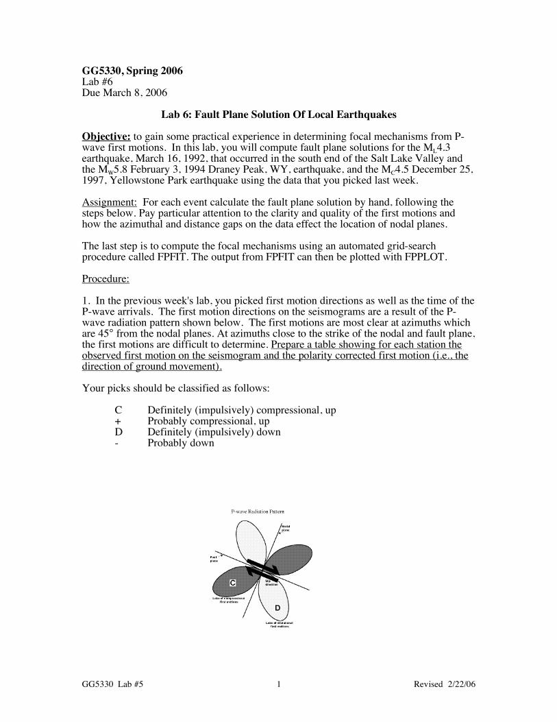
Lab 6: Fault Plane Solution Of Local Earthquakes Objective: to gain some practical experience in determining focal mechanisms from P-wave first motions. In this lab, you will compute fault plane solutions for the ML4.3 earthquake, March 16, 1992, that occurred in the south end of the Salt Lake Valley and the MW5.8 February 3, 1994 Draney Peak, WY, earthquake, and the MC4.5 December 25, 1997, Yellowstone Park earthquake using the data that you picked last week. Assignment: For each event calculate the fault plane solution by hand, following the steps below. Pay particular attention to the clarity and quality of the first motions and how the azimuthal and distance gaps on the data effect the location of nodal planes. The last step is to compute the focal mechanisms using an automated grid-search procedure called FPFIT. The output from FPFIT can then be plotted with FPPLOT. Procedure: 1. In the previous week's lab, you picked first motion directions as well as the time of the P-wave arrivals. The first motion directions on the seismograms are a result of the P-wave radiation pattern shown below. The first motions are most clear at azimuths which are 45° from the nodal planes. At azimuths close to the strike of the nodal and fault plane, the first motions are difficult to determine. Prepare a table showing for each station the observed first motion on the seismogram and the polarity corrected first motion (i.e., the direction of ground movement). Your picks should be classified as follows: C Definitely (impulsively) compressional, up + Probably compressional, up D Definitely (impulsively) down - Probably down

GG5330 Lab #5 2 Revised 2/22/06

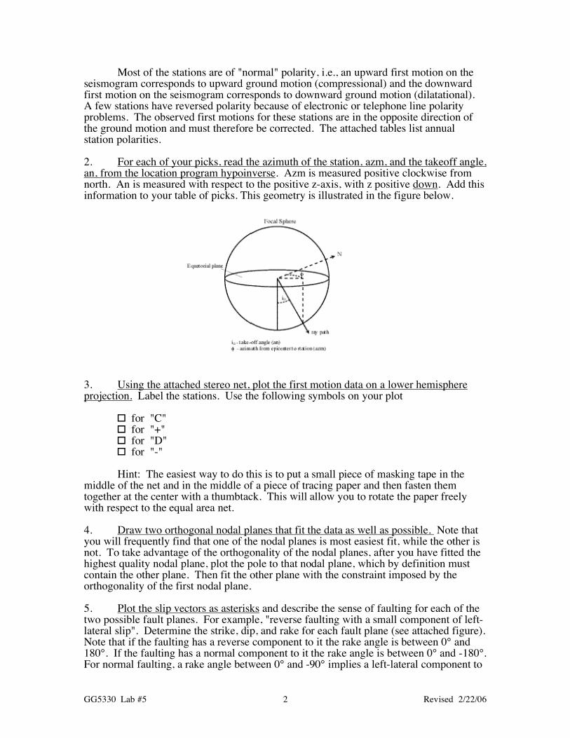
Most of the stations are of "normal" polarity, i.e., an upward first motion on the seismogram corresponds to upward ground motion (compressional) and the downward first motion on the seismogram corresponds to downward ground motion (dilatational). A few stations have reversed polarity because of electronic or telephone line polarity problems. The observed first motions for these stations are in the opposite direction of the ground motion and must therefore be corrected. The attached tables list annual station polarities. 2. For each of your picks, read the azimuth of the station, azm, and the takeoff angle, an, from the location program hypoinverse. Azm is measured positive clockwise from north. An is measured with respect to the positive z-axis, with z positive down. Add this information to your table of picks. This geometry is illustrated in the figure below.

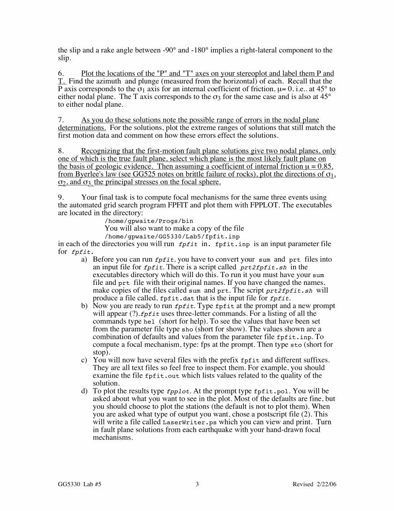
3. Using the attached stereo net, plot the first motion data on a lower hemisphere projection. Label the stations. Use the following symbols on your plot � for "C" � for "+" � for "D" � for "-" Hint: The easiest way to do this is to put a small piece of masking tape in the middle of the net and in the middle of a piece of tracing paper and then fasten them together at the center with a thumbtack. This will allow you to rotate the paper freely with respect to the equal area net. 4. Draw two orthogonal nodal planes that fit the data as well as possible. Note that you will frequently find that one of the nodal planes is most easiest fit, while the other is not. To take advantage of the orthogonality of the nodal planes, after you have fitted the highest quality nodal plane, plot the pole to that nodal plane, which by definition must contain the other plane. Then fit the other plane with the constraint imposed by the orthogonality of the first nodal plane. 5. Plot the slip vectors as asterisks and describe the sense of faulting for each of the two possible fault planes. For example, "reverse faulting with a small component of left-lateral slip". Determine the strike, dip, and rake for each fault plane (see attached figure). Note that if the faulting has a reverse component to it the rake angle is between 0° and 180°. If the faulting has a normal component to it the rake angle is between 0° and -180°. For normal faulting, a rake angle between 0° and -90° implies a left-lateral component to

GG5330 Lab #5 3 Revised 2/22/06

the slip and a rake angle between -90° and -180° implies a right-lateral component to the slip. 6. Plot the locations of the "P" and "T" axes on your stereoplot and label them P and T. Find the azimuth and plunge (measured from the horizontal) of each. Recall that the P axis corresponds to the σ1 axis for an internal coefficient of friction, µ= 0, i.e.. at 45° to either nodal plane. The T axis corresponds to the σ3 for the same case and is also at 45° to either nodal plane. 7. As you do these solutions note the possible range of errors in the nodal plane determinations. For the solutions, plot the extreme ranges of solutions that still match the first motion data and comment on how these errors effect the solutions. 8. Recognizing that the first-motion fault plane solutions give two nodal planes, only one of which is the true fault plane, select which plane is the most likely fault plane on the basis of geologic evidence. Then assuming a coefficient of internal friction µ = 0.85, from Byerlee's law (see GG525 notes on brittle failure of rocks), plot the directions of σ1, σ2, and σ3, the principal stresses on the focal sphere. 9. Your final task is to compute focal mechanisms for the same three events using the automated grid search program FPFIT and plot them with FPPLOT. The executables are located in the directory:

/home/gpwaite/Progs/bin You will also want to make a copy of the file /home/gpwaite/GG5330/Lab5/fpfit.inp in each of the directories you will run fpfit in. fpfit.inp is an input parameter file for fpfit.

a) Before you can run fpfit, you have to convert your sum and prt files into an input file for fpfit. There is a script called prt2fpfit.sh in the executables directory which will do this. To run it you must have your sum file and prt file with their original names. If you have changed the names, make copies of the files called sum and prt. The script prt2fpfit.sh will produce a file called, fpfit.dat that is the input file for fpfit.

b) Now you are ready to run fpfit. Type fpfit at the prompt and a new prompt will appear (?).fpfit uses three-letter commands. For a listing of all the commands type hel (short for help). To see the values that have been set from the parameter file type sho (short for show). The values shown are a combination of defaults and values from the parameter file fpfit.inp. To compute a focal mechanism, type: fps at the prompt. Then type sto (short for stop).

c) You will now have several files with the prefix fpfit and different suffixes. They are all text files so feel free to inspect them. For example, you should examine the file fpfit.out which lists values related to the quality of the solution.

d) To plot the results type fpplot. At the prompt type fpfit.pol. You will be asked about what you want to see in the plot. Most of the defaults are fine, but you should choose to plot the stations (the default is not to plot them). When you are asked what type of output you want, chose a postscript file (2). This will write a file called LaserWriter.ps which you can view and print. Turn in fault plane solutions from each earthquake with your hand-drawn focal mechanisms.

GG5330 Lab #5 4 Revised 2/22/06