globally coupled oscillator networks

This is page 1Printer: Opaque this

Globally Coupled OscillatorNetworks

Eric Brown1

Philip Holmes1,2

Jeff Moehlis1

1 Program in Applied and Computational Mathematics,2 Department of Mechanical and Aerospace Engineering,Princeton University, Princeton, NJ 08544, U.S.A.

ABSTRACT We study a class of permutation-symmetric globally-coupled,phase oscillator networks on N -dimensional tori. We focus on the effectsof symmetry and of the forms of the coupling functions, derived from un-derlying Hodgkin-Huxley type neuron models, on the existence, stability,and degeneracy of phase-locked solutions in which subgroups of oscillatorsshare common phases. We also estimate domains of attraction for the com-pletely synchronized state. Implications for stochastically forced networksand ones with random natural frequencies are discussed and illustrated nu-merically. We indicate an application to modeling the brain structure locus

coeruleus: an organ involved in cognitive control.

1 Introduction and background

We consider networks of N rotator oscillators with constant forcing andpairwise phase-difference and absolute-phase ‘product’ coupling, describedby:

θi = ωi +1

N

N∑

j=1

αijfij(θj − θi) + hi(θi)1

N − 1

N∑

j 6=i

βijgj(θj), (1.1)

where (θ1, . . . , θN )T ∈ TN , αij , βij and fij , hi, gj are, respectively, couplingparameters and 2π-periodic functions, and ωi are the natural frequenciesof the uncoupled rotators. This paper focuses on networks with identical

2 Eric Brown, Philip Holmes and Jeff Moehlis

global (mean field) coupling, so that equation (1.1) becomes

θi = ω +α

N

N∑

j=1

f(θj − θi) + h(θi)β

N − 1

N∑

j 6=i

g(θj) , (1.2)

although we include some results with randomly distributed frequenciesωi, and also with additive random noise. The denominators (N , N −1) areintroduced to normalize coupling effects.

Rotator (phase-only) models of coupled oscillators have been widely stud-ied, especially in the contexts of neuroscience and coupled Josephson junc-tions. The phase equations offer, respectively, significant simplification ofmore realistic neuron models of Hodgkin-Huxley or Fitzhugh-Nagumo type:see e.g. Murray [2001]; Keener and Sneyd [1998]; Hoppensteadt and Izhike-vich [1997], and of the Josephson circuit equations: e.g. Watanabe and Stro-gatz [1994]; Watanabe and Swift [1997]; Wiesenfeld, Colet, and Strogatz[1998]. In the case that the N uncoupled oscillators have strongly attractinglimit cycles in their full phase space, the persistence of normally hyperbolicinvariant manifolds (Fenichel [1971]) under small perturbations (weak cou-pling) may be used to reduce the system to the N -torus by a suitablecoordinate transformation. Two procedures for approximating the reducedsystem will be applied in Section 4 of this paper. The first is the ‘strongattraction’ (SA) method described in Ermentrout and Kopell [1990] andHoppensteadt and Izhikevich [1997]; the second, a related ‘phase response’(PR) technique, is given in e.g. Ermentrout [1996], Kuramoto [1997], andKim and Lee [2000].

We were motivated to study systems of the form (1.1) by the study ofUsher, Cohen, Servan-Schreiber, Rajkowski, and Aston-Jones [1999], whichpresents data showing that neurons of the brain organ locus coeruleus (LC)in monkeys exhibit two distinct firing patterns corresponding to differentbehaviors evinced in cognitive tasks, cf. Grant, Aston-Jones, and Redmond[1988]; Aston-Jones, Rajkowski, and Alexinsky [1994]. These are designatedas the phasic and tonic modes. In the latter, associated with labile behav-ior and poor task performance, LC neurons fire at a relatively high rate,but with little synchrony; in the former, associated with good performance,their average firing rate is lower but they display greater synchrony (i.e.higher correlation among individual firing times). See Figure 1.1(a). More-over, firing patterns are more responsive to changes in stimulus in thephasic than in the tonic mode; see Figure 1.1(b,c). Thus, the LC has beenproposed as a modulator involved in cognitive control, cf. Servan-Schreiber,Printz, and Cohen [1990].

The computational model constructed in Usher, Cohen, Servan-Schreiber,Rajkowski, and Aston-Jones [1999] includes inhibitory synaptic and exci-tatory electrotonic coupling (Johnston and Wu [1997]), explicitly imposedrefractory periods, and representations of rapid depolarization during ac-tion potentials to successfully reproduce these characteristics of the phasic

1. Globally Coupled Oscillator Networks 3

��

��

��

��

��

FIGURE 1.1. Reproduced from Usher, Cohen, Servan-Schreiber, Rajkowski, andAston-Jones [1999], with adapted caption. (a) Cross correlograms for two simul-taneously recorded LC neurons during phasic LC mode (filled histogram) andtonic mode (line): central peak indicates increased synchrony in phasic mode.(b,c) Histograms of LC activity in phasic (b) and tonic (c) LC modes: psy-chological stimulus onset (which precedes the direct stimulus I(t) considered inSection 4.4) is marked by dotted line, and enhanced response in phasic versustonic mode is apparent. Average firing rate is lower in phasic mode.

and tonic modes; transitions between the two modes are effected by vary-ing the degree of electrotonic coupling. However, the model’s complexitymakes analysis difficult, and we wish to develop a model that has similarbehavior but is more amenable to mathematical study.

In this paper, we consider coupling functions motivated by two physi-cally distinct mechanisms: (1) electrotonic or gap junction coupling, basedon voltage differences between cells in electrical contact, and (2) spike-triggered synaptic transmission that releases a pulse of neurotransmitteracross synaptic clefts. Electrotonic coupling is additive in the sense that thesum of voltage differences of all cells in contact with a given cell influencethat cell; hence the first sum in equations (1.1) and (1.2). Synaptic cou-pling leads to absolute phase terms βhi(θi)gj(θj) in (1.1-1.2). Intuitively,these arise because the primary effect on the post-synaptic cell occurs afterthe pre-synaptic cell fires, and therefore depends, via g(θj), on the latter’slocation on its phase circle. Coupling via a ‘reversal potential’ also dependsupon the post-synaptic cell’s phase through h(θi) (Ermentrout and Kopell[1990]; Taylor and Holmes [1998]); thus h(θi) multiplies the summed g(θj)’s,leading to the product coupling form of the second term.

We furthermore assume an additional separation of scales, taking elec-trotonic coupling to be weaker than synaptic, so that it can be averaged togive the phase-difference functions αfij without affecting βhigj at leading


order; we are currently studying when the standard averaging theorems canbe extended to make this rigorous. Sections 3 and 4 consider the dynamicsof equation (1.1) for various values of α and β, without a priori restrictingto the |α| ¿ |β| ¿ O(1) required in this derivation of the phase equations.

When β = 0 but frequencies differ between oscillators, equation (1.2) isreferred to as the Kuramoto model (Kuramoto [1984]), on which there isan extensive literature; see the recent review of Strogatz [2000] and refer-ences therein (e.g. Crawford [1995]). Much of this work has been done inthe continuum limit N → ∞, and Strogatz [2000] adopts this viewpoint;specifically, stability analyses of some stationary (continuous) states arediscussed. Finite-dimensional results, including a Liapunov function anddimension reduction, are found in the context of Josephson junction mod-els in Watanabe and Strogatz [1994]. Many earlier studies take only theleading term in an odd Fourier expansion of f , so that f(·) = sin(·); aswe shall see this is a very degenerate case for the mean field coupled sys-tem (1.2) (e.g. Nichols and Wiesenfeld [1992]; Golomb, Hansel, Shraiman,and Sompolinsky [1992]). Moreover, as shown in Izhikevich [2000], relax-ation oscillators of Hodgkin-Huxley or Fitzhugh-Nagumo type lead to muchricher phase difference functions than sin(·). Others have recognized the im-portance of higher Fourier harmonics: see Daido [1994]; Golomb, Hansel,Shraiman, and Sompolinsky [1992]; Nichols and Wiesenfeld [1992]; Watan-abe and Swift [1997]. Additional work on finite dimensional oscillator net-works includes Kopell and Ermentrout [1990]; Kopell, Ermentrout, andWilliams [1991]; Kopell and Ermentrout [1994], which consider directedcoupling, Bressloff and Coombes [1998], which considers integrate-and-firemodels derived from coupled spiking neurons, and Okuda [1993], whichwill be discussed in Section 2. Shortly before this paper was submitted,we learned of recent work of Chow and Kopell [2000], in which the effectsof spike shape on electrotonically coupled integrate-and-fire networks arestudied. They find that the existence and stability of splay states dependson the spike shape in a manner that would be interesting to compare withthe present results.

The present paper draws on Ashwin and Swift [1992], which addressesa class of SN × T 1-equivariant oscillator networks (of which (1.2) is anexample when β = 0). We now summarize the properties of symmetricdynamical systems necessary to present and apply these results; for morebackground, see Golubitsky, Stewart, and Schaeffer [1988].

Consider the ODE

dx

dt= f(x) , x ∈ manifoldM , (1.3)

and let Γ be a group acting on M . The ODE is said to be Γ-equivariant iff commutes with the group action, i.e.

f(γx) = γf(x) ∀γ ∈ Γ, x ∈M , (1.4)


where the derivative map γ (Arnold [1973]) acts on the tangent space TM ;for linear actions of γ, γ = γ. The symmetry of a solution x0 ∈ M ischaracterized by the isotropy subgroup Σx0

= {γ ∈ Γ : γx0 = x0}, thatis, the set of all group elements which leave the solution x0 unchanged.Associated with an isotropy subgroup is a fixed point subspace Fix[Σx0

] ={x ∈ M : σx = x ∀σ ∈ Σx0

}: the set of points fixed by all elements ofΣx0

. Two immediate consequences of Γ-equivariance are that (1) for anysolution x(t) to equation (1.3), γx(t) is also a solution, and (2) fixed-pointsubspaces are invariant under the flow generated by f . We will refer to thislatter property as dynamical invariance. As in Ashwin and Swift [1992], westudy special classes of symmetric systems defined by the following groups:the circle group T 1 = {δ : δ ∈ [0, 2π)} (with action on TN , θi 7→ θi+δ, ∀ i),the cyclic subgroups Zm ∈ T 1 (with action θi 7→ θi + 2π/m), and thesubgroups of permutations on j-many coordinates, Sj .

The remainder of the paper proceeds as follows. In Section 2 we study(1.2) with β = 0 (SN×T

1 equivariant), emphasizing the influence of generalcoupling functions and obtaining additional results for odd functions f . Insucceeding sections the symmetries are gradually relaxed. In Section 3 thisis done by breaking T 1 equivariance through re-introduction of h(θi)g(θj)terms. In Section 4 we break SN equivariance by introducing a random dis-tribution of frequencies as well as random excitation, and apply our modelto the LC. Thus, Sections 2 and 3 are largely abstract and general, whileSection 4 concerns specific ‘neural’ coupling. Conclusions are drawn and fu-ture directions noted in Section 5. Our major contributions to this surveyon globally coupled oscillators include the implications of gradient dynam-ics for the existence of families of equilibria, nonlinear stability results forthe synchronized state, and the analysis of a two-parameter (α, β) system,including the influence of noise, in relation to the LC model.

2 SN × T 1 phase difference oscillator systems

This section treats the system of N oscillators,

θi = ω +α

N

N∑

j=1

f (θj − θi) , i = 1, . . . , N, (2.1)

where f(·) is assumed to be continuously differentiable and 2π-periodic.Transforming to coordinates φi = θi−ωt rotating with the common naturalfrequency, equation (2.1) becomes

φi =α

N

N∑

j=1

f (φj − φi) . (2.2)


Denoting the phase differences φj − φi ≡ φji, we seek ‘diagonal flow’ peri-odic solutions φ of equation (2.2) in the form

˙φi =1

N

N∑

j=1

f(φji

)= c, i = 1, . . . , N, (2.3)

where c is a constant, nonzero in general. These solutions are also peri-odic for (2.1), and, employing a second rotating frame θi − (ω + c)t, theybecome fixed points. Since the derivatives f ′(φji) are time-independent,eigenvalue calculations suffice to determine the stability of such solutions.Equation (2.3) determines the N −1 phase differences, without loss of gen-erality leaving the phase φ1 unspecified, as expected from the T 1 symmetryof equation (2.1).

We began this work by determining the existence and stability of diagonalflow solutions to equation. (2.2). While we later found many of the followingresults in the literature, no unified presentation appears to exist, so weprovide a summary here, including extensions and new examples of ourown. Proofs are only sketched.

2.1 Gradient property for odd phase-difference

coupling

If f(·) is odd, we observe as in Theorem 9.15 of Hoppensteadt and Izhike-vich [1997] that:

2.1 Proposition. Equation (2.2) is a gradient dynamical system on TN

with potential

V =α

N

N−1∑

i=1

N∑

j=i+1

F (φj − φi), where f(θ) = F ′(θ). (2.4)

Proof. Note that

−∂V

∂φi=

α

N

∑

j<i

f(φj − φi)−α

N

∑

j>i

f(φi − φj); (2.5)

the oddness of f implies that φi = −∂V/∂φi. ¥

Proposition 2.1 implies that

V =

N∑

i=1

∂V

∂φiφi = −

N∑

i=1

φ2i ≤ 0 , (2.6)

with equality only at equilibria. Thus, equation (2.2) with odd f(·) has noperiodic or homoclinic orbits or heteroclinic cycles: all solutions approachequilibria, and almost all approach stable equilibria. In particular,

2.2 Corollary. For f odd, equation (2.3) has no solutions unless c = 0.


2.2 Periodic orbits for the phase difference system

k

k

k

k

k

k

N-p

p

N

a) b) c)

k1

k2

φ1

d)

δ

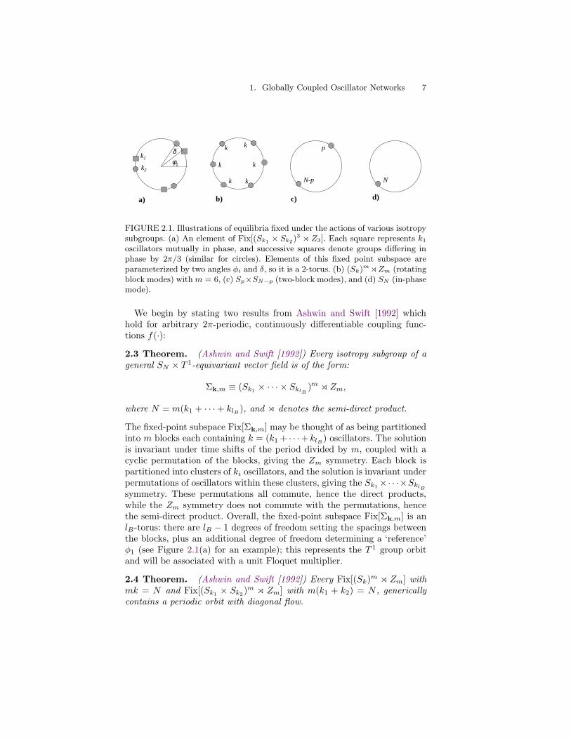
FIGURE 2.1. Illustrations of equilibria fixed under the actions of various isotropysubgroups. (a) An element of Fix[(Sk1 × Sk2)

3 o Z3]. Each square represents k1

oscillators mutually in phase, and successive squares denote groups differing inphase by 2π/3 (similar for circles). Elements of this fixed point subspace areparameterized by two angles φi and δ, so it is a 2-torus. (b) (Sk)

moZm (rotatingblock modes) withm = 6, (c) Sp×SN−p (two-block modes), and (d) SN (in-phasemode).

We begin by stating two results from Ashwin and Swift [1992] whichhold for arbitrary 2π-periodic, continuously differentiable coupling func-tions f(·):

2.3 Theorem. (Ashwin and Swift [1992]) Every isotropy subgroup of ageneral SN × T

1-equivariant vector field is of the form:

Σk,m ≡ (Sk1 × · · · × SklB)m o Zm,

where N = m(k1 + · · ·+ klB ), and o denotes the semi-direct product.

The fixed-point subspace Fix[Σk,m] may be thought of as being partitionedinto m blocks each containing k = (k1+ · · ·+ klB ) oscillators. The solutionis invariant under time shifts of the period divided by m, coupled with acyclic permutation of the blocks, giving the Zm symmetry. Each block ispartitioned into clusters of ki oscillators, and the solution is invariant underpermutations of oscillators within these clusters, giving the Sk1×· · ·×SklB

symmetry. These permutations all commute, hence the direct products,while the Zm symmetry does not commute with the permutations, hencethe semi-direct product. Overall, the fixed-point subspace Fix[Σk,m] is anlB-torus: there are lB − 1 degrees of freedom setting the spacings betweenthe blocks, plus an additional degree of freedom determining a ‘reference’φ1 (see Figure 2.1(a) for an example); this represents the T 1 group orbitand will be associated with a unit Floquet multiplier.

2.4 Theorem. (Ashwin and Swift [1992]) Every Fix[(Sk)m o Zm] with

mk = N and Fix[(Sk1 × Sk2)m o Zm] with m(k1 + k2) = N , generically

contains a periodic orbit with diagonal flow.


Ashwin and Swift [1992] prove this theorem by noting that, without lossof generality, the phases of the oscillators can be ordered as φ1 ≤ φ2 ≤· · · ≤ φN ≤ φ1+2π. The oscillators retain their ordering under the dynam-ics, i.e., they can never ‘pass’ each other, since this would involve crossingan invariant fixed-point subspace. Projecting the phases onto the manifoldφ1 = 0 (by subtracting the instantaneous value of φ1 from each phase) givesa simplex called the ‘canonical invariant region’ (CIR). The intersection ofFix[(Sk)

m o Zm] with the CIR is a zero-dimensional invariant subspace,i.e., an equilibrium. In the unprojected system, this corresponds to a pe-riodic orbit (or a circle of equilibria if φ1 = 0 for all time) with isotropy(Sk)

m oZm. Furthermore, the intersection of Fix[(Sk1 ×Sk2)m oZm] with

the CIR is a one-dimensional line segment. The end points of this segmenthave isotropy (Sk1+k2)

m o Zm, and are equilibria with stability in the di-rection of the line segment determined by the same eigenvalue. Providedthis eigenvalue does not vanish (this is the nondegeneracy condition satis-fied for generic functions f), this can only happen if there is at least oneequilibrium in the interior of the line segment. In the original system, thiscorresponds to a periodic orbit (or one-torus of equilibria if φ1 = 0 for alltime) with isotropy (Sk1 ×Sk2)

moZm. If k1 = k2, the midpoint of the linesegment is an equilibrium with isotropy (Sk1)

2m o Z2m; this can serve asthe necessary equilibrium in the interior of the line segment.

Ashwin and Swift [1992] developed their proof for systems coupled withgeneral T 1-equivariant functions. The special additive, pairwise-coupledform of the coupling in (2.1) allows a much simpler argument to prove(a restricted version of) Theorem 2.4. For a (Sk1 × Sk2)

m o Zm solutionwith clusters separated by phase δ (see Figure 2.1(a)) to have diagonal flowrequires φi ≡ c(δ) ∀i, for some fixed δ. This condition reduces to

c1(δ) = c2(δ) , where (2.7)

c1(δ) = k1

m−1∑

j=0

f

(2πj

m

)+ k2

m−1∑

j=0

f

(2πj

m+ δ

)(2.8)

c2(δ) = k2

m−1∑

j=0

f

(2πj

m

)+ k1

m−1∑

j=0

f

(2πj

m− δ

)(2.9)

are the (constant) phase velocities for oscillators in k1 or k2-clusters, re-spectively (cf. Kim and Lee [2000] for m = 1). A quick sketch shows that atleast one δ ∈ (0, 2π/m) satisfying (2.7) must exist if c′1(0)/k2 = −c′2(0)/k1is nonzero, since c′1,2(0) = c′1,2(2π/m). Thus, the nondegeneracy condition

becomes∑m−1j=0 f ′( 2πj

m) 6= 0; for SN−p × Sp solutions, m = 1, implying

f ′(0) 6= 0. Further, for (Sk)m o Zm rotating blocks the equality φi ≡ γ

is automatic. Finally, we note that if k1 = k2, δ = π/m always satisfies


(2.7), so that the corresponding (Sk1×Sk1)moZm solutions may also have

symmetry (Sk1)2m o Z2m.

These arguments extend in a natural way to show the existence of weaksolutions to the partial differential equations derived from (2.1) as N →∞(Crawford and Davies [1999]). These are symmetrically-spaced combina-tions of delta distributions rotating at the frequency c(δ) found above, withthe kj-cluster distributions weighted by kj(N)/m(k1(N)+k2(N)), j = 1, 2.Here, kj(N) is the number of oscillators in a cluster when the total numberof oscillators is N , and the N → ∞ limit is taken over a subsequence ofconfigurations (E [2001]) with constant kj(N)/m(k1(N)+k2(N)) such thatm (fixed) divides k1(N)+k2(N). Under the same nondegeneracy conditionsas above, their existence may be shown for any values of kj/m(k1 + k2)and any m. Furthermore, if f lacks m-th Fourier harmonics and their mul-tiples, families of Zm-symmetric solutions analogous to the fixed tori ofSection 2.4 also exist. A study of the stability of these solutions, their per-sistence under the introduction of a (diffusive) noise term, and associatedconvergence issues as N →∞ is in progress.

For the special case of odd phase-difference coupling, Proposition 2.1ensures:

2.5 Theorem. For the phase-difference system (2.2) with f odd, everyFix[(Sk1 × · · ·×SklB

)m oZm] with m(k1+ · · ·+ klB ) = N contains at leastone equilibrium.

Proof. Let Vk,m denote the restriction of V from (2.4) to the lB-torus

Σk,m. Vk,m is a continuous function on the (flow-invariant) compact setΣk,m and thus possesses a minimum φ on Σk,m. Consider a trajectory

φ(t) ∈ Σk,m starting at φ at t = 0. Since V = −∑Ni=1 φi

2, if φ(t) 6= φ

then V (φ(t)) < V (φ), ∀t > 0. This contradicts the assumption that φ is aminimum for V, so φ ∈ Σk,m must be a fixed point for equation (2.2). ¥

Associated with any of the equilibria above, we expect at least one zeroeigenvalue and a circle of equilibria corresponding to its T 1 group orbit.

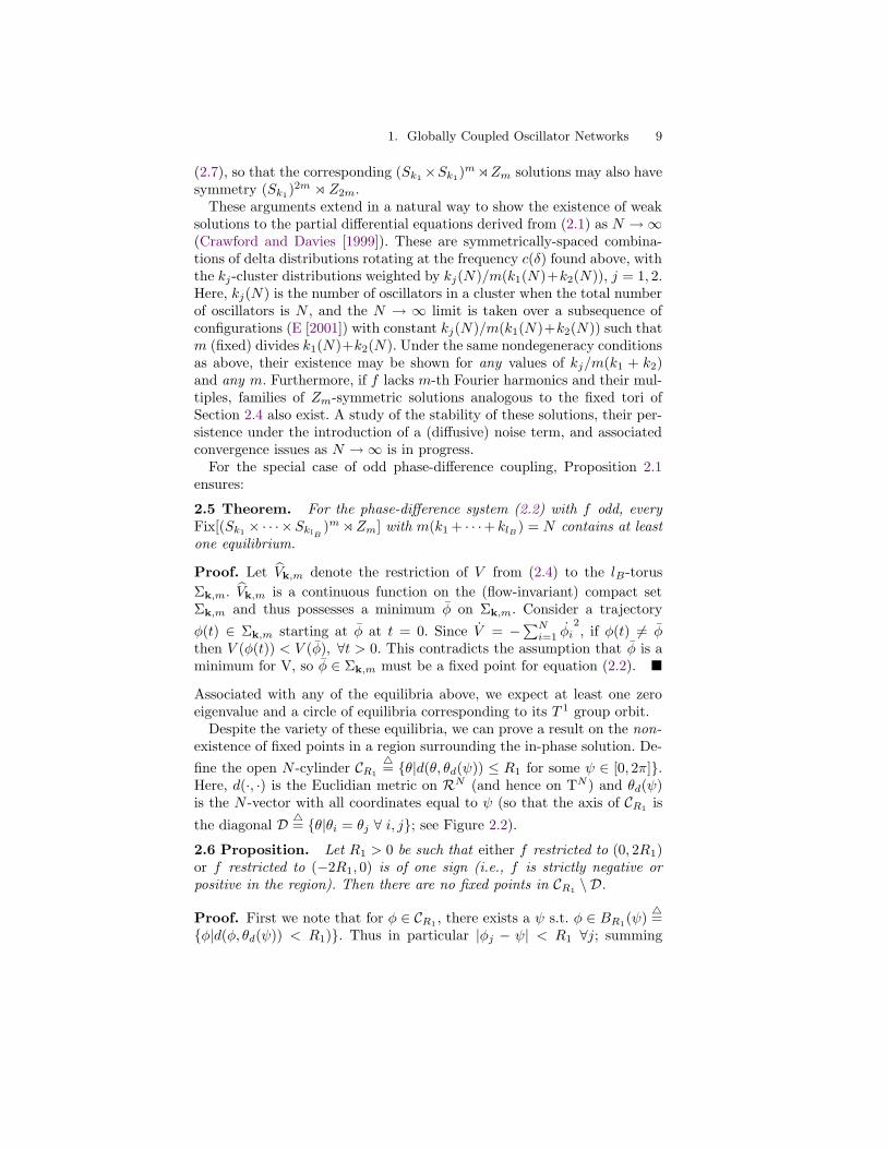
Despite the variety of these equilibria, we can prove a result on the non-existence of fixed points in a region surrounding the in-phase solution. De-

fine the open N -cylinder CR1

4= {θ|d(θ, θd(ψ)) ≤ R1 for some ψ ∈ [0, 2π]}.

Here, d(·, ·) is the Euclidian metric on RN (and hence on TN ) and θd(ψ)is the N -vector with all coordinates equal to ψ (so that the axis of CR1

is

the diagonal D4= {θ|θi = θj ∀ i, j}; see Figure 2.2).

2.6 Proposition. Let R1 > 0 be such that either f restricted to (0, 2R1)or f restricted to (−2R1, 0) is of one sign (i.e., f is strictly negative orpositive in the region). Then there are no fixed points in CR1

\ D.

Proof. First we note that for φ ∈ CR1, there exists a ψ s.t. φ ∈ BR1

(ψ)4=

{φ|d(φ, θd(ψ)) < R1)}. Thus in particular |φj − ψ| < R1 ∀j; summing


two of these inequalities and applying the triangle inequality gives |φji| <2R1 ∀ i, j. Next, consider an arbitrary N -vector φ ∈ CR1

\ D, where with-out loss of generality φ1 ≤ φ2 ≤ · · · ≤ φN . If the chosen interval in thehypothesis is (0, 2R1), note that 2R1 > φj−φ1 ≥ 0 ∀ j and φj−φ1 > 0 for

at least one j (since φ /∈ D). Thus, φ1 = αN

∑Nj=1 f(φj − φ1) 6= 0, because

each term in the sum is either zero or of the same sign (the continuity of fimplies that f(0) is either 0 or of the same sign as f(φ) for φ ∈ (0, 2R1))and at least one term is nonzero. If the chosen interval is (−2R1, 0), we usethe facts that 0 ≥ φj − φN > −2R1 ∀ j and φj − φN < 0 for at least one

j. Similarly, then, ˙φN = αN

∑Ni=1 f(φj − φN ) 6= 0. Hence φ is not a fixed

point. ¥

This result does not exclude orbits with nonzero diagonal flow, which mayexist within CR1

\ D if f is not odd.We now consider the stability of some of the solutions found above.

C

D

FIGURE 2.2. The diagonal D and cylinder C of Proposition 2.6. The cube rep-resents the N -torus.

2.3 Stability of periodic orbits

Rotating blocks

We study solutions with isotropy (Sk)moZm (rotating block modes), Sp×

SN−p (two-block modes), and SN (in-phase mode). Since the Jacobianis constant along these periodic orbits with diagonal flow, this problemreduces to computation of eigenvalues (Ashwin and Swift [1992]). Stabilitywill be discussed in terms of orbital stability, which implies asymptoticstability with respect to all perturbations transverse to the (continuous)T 1 group orbit of the solution (hence excluding the corresponding zeroeigenvalue). Note that if c 6= 0 in equation (2.3), the group orbit andperiodic orbit coincide.

To state some of the stability results, it is useful to express the coupling


function in a Fourier series with coefficients bol and bel :

f(φji) =∞∑

l=0

(bol sin(lφji) + bel cos(lφji)) . (2.10)

For (Sk)m o Zm symmetric solutions we have, as in Okuda [1993] and

(for m = 1) Watanabe and Swift [1997]:

2.7 Proposition. Let N = mk and let φ be an (Sk)m o Zm-invariant

fixed point or periodic orbit with diagonal flow. Then the eigenvalues of theJacobian J(φ) obtained by linearization of Equation (2.2) are

λ = λ0 = 0, with multiplicity 1λ = λjr, j = 1, ...,m− 1 : ‘rotation eigenvalues’λ = λp, with multiplicity m(k − 1) : ‘permutation eigenvalues’

,

λjr =α

m

m−1∑

k=1

f ′(2πk

m

)(exp

(2πkji

m

)− 1

)

=α

2

∑

l∈M(m)j1

l (bol + ibel ) +∑

l∈M(m)j2

l (bol − ibel )− 2

∑

l∈M(m)

lbol

(2.11)

λp = −α

m

m−1∑

k=0

f ′(2πk

m

)= −α

∑

l∈M(m)

bol l, (2.12)

M(m)j1 = {mh− j|h = 1, 2, ...} , M(m)j2 = {mh+ j|h = 0, 1, 2, ...} ,

M(m) = {mh|h = 1, 2, ...} .

The ‘rotation’ and ‘permutation’ terminology is due to Ashwin and Swift[1992], where general formulae for eigenvalues and eigenvectors are pre-sented. The proof of Proposition 2.7 repeatedly uses the following simplefact. Define the setM = {l|l = qm for some q ∈ Z} and let γ = exp(2πi/m);

then for l ∈ Z\M,∑m−1r=1 γ lr = −1. From here, them×m-blocked structure

of the Jacobian along with results on the eigenvectors of Toeplitz matricesleads to the desired conclusion.

If m = 1, then the proposition addresses the SN -invariant (in-phase) so-lutions. Here there are no rotation eigenvalues, and the permutation eigen-values are simply

λp = −αf′(0) , (2.13)

with multiplicity N−1. Nonlinear stability of these solutions is discussed inSection 3.2 (Proposition 3.2 with β = 0). At the other extreme, if m = N ,


the proposition addresses the ZN -invariant solutions in which the phasesof the oscillators are equally spaced; these are called ‘rotating wave’ solu-tions by Ashwin and Swift [1992], and correspond to the ‘splay state’ inthe Josephson junction literature. In this case, there are no permutationeigenvalues, and (2.11) reduces to equation (63) of Watanabe and Swift[1997].

We now give examples to illustrate several interesting stability behavioursimplied by Proposition 2.7. Including only the first harmonic in the cou-pling function (f(·) = bo1 sin(·) + be1 cos(·)), we have for m > 1:

λp = 0,with multiplicity m(k − 1)

λjr =

{α2 (b

o1 − ib

e1) and

α2 (b

o1 + ibe1) for j = 1 and m− 1

0 otherwise (multiplicity m− 3),

in addition to λ0. In this case the (Sk)m o Zm solutions are highly degen-

erate and, for αbo1 > 0, unstable. For m = N (k = 0), there are N − 2 zeroeigenvalues. This result is well-known from the Josephson junction liter-ature; in Watanabe and Strogatz [1994], it is shown to be related to theintegrability of the equations for this choice of f .

On the other hand, we note that inclusion of higher harmonics in f(·)generically unfolds the degeneracy in the sense that all but one (λ0) of theeigenvalues become nonzero, implying instability or orbital stability. Forexample, adding themth harmonic (f(·) = bo1 sin(·)+b

e1 cos(·)+b

om sin(m·)+

bem cos(m·); m 6= 1), we obtain

λp = −αbomm, with multiplicity m(k − 1)

λjr =

{α[ 12 (b

o1 − ib

e1)− b

omm], c.c. if j = 1, m− 1

−αbomm otherwise (multiplicity m− 3),

so that any (Sk)m o Zm solution is orbitally stable if αbom > α

bo1

2m andαbom > 0. We also note that for coupling functions whose harmonic indicesbelong entirely toM(l), any oscillator may be individually translated froma (Sk)

moZm solution by a multiple of 2πlto give another equilibrium. These

translations give a total of lN fixed points, each with identical stability (dueto the 2π

lperiodicity of f).

The calculations proving Proposition 2.7 show which eigenvectors corre-spond to zero eigenvalues and hence along which directions there may becontinuous families of equilibria. For example, with k = 1, m = N = 4 andf(·) = sin(·), the nondiagonal zero eigenvector is (1,−1, 1,−1)T, which re-flects the fact that equilibrium is preserved if ‘diametrically-opposite’ pairsof oscillators are rotated independently.

Two-block periodic orbits

For f ′(0) 6= 0, equation (2.13) guarantees that the SN -invariant solutionssatisfy the nondegeneracy assumption of Theorem 2.4. Then, the Theorem


(with m = 1) implies that for some δ(p) > 0, equation (2.2) has periodicorbits with φji ∈ {0, δ(p), 2π − δ(p)} for all i, j. This occurs when twoblocks of p and N − p identical-phase oscillators are mutually out of phaseby δ; to avoid redundancy, we restrict 0 ≤ p ≤ bN/2c. The Jacobian fromlinearizing around a SN−p×Sp solution has a four-blocked structure whichyields:

2.8 Proposition. (Kim and Lee [2000]) Let φ be an (Sp×SN−p)-invariantsolution and 0 ≤ p ≤ bN/2c. Then for p ≥ 1 the eigenvalues of the Jacobianfrom equation (2.2) are:

λ1 = α(b− pN(a+ b)), with multiplicity p− 1

λ2 = α( pN(a+ c)− a), with multiplicity N − p− 1

λ3 = 0, with multiplicity 1

λ4 = α(N−pN

b+ pNc), with multiplicity 1

. (2.14)

Here, a = f ′(0), b = −f ′(δ(p)), c = −f ′(−δ(p)).

If f(·) is odd, two-block states with δ = π exist for any p since f(0) =f(π) = 0; we write δ 6= δ(p) to indicate this p-independence of δ. Oddnessof f also implies b = c. This case was studied in Okuda [1993], whereexpressions corresponding to (2.14) are presented.

2.9 Corollary. Assume that b = c, δ 6= δ(p), and that a, b > 0. If α > 0,the two-block equilibria of equation (2.2) are orbitally stable if and onlyif p = 0. If α < 0, the equilibria are stable if and only if p 6= 0 anda < bp/(N − p), if the equilibria are stable for p = k for some k ≤ bN/2c,then they are stable for p > k.

Proof. The results for α > 0 are immediate from λ4 of equation (2.14)and (2.13). For α < 0, we note that λ1,2 ≤ 0 implies Na ≤ p(a+ b) ≤ Nb.Upon rearranging, this yields a ≤ b(N − p)/p and a ≤ bp/(N − p); for pin the given range, the latter inequality implies the first, and for fixed aand b it is clear that if the second inequality is satisfied for p = k, then itcontinues to be satisfied as p increases. In this case λ1, λ2 and λ4 are allstrictly negative, leading to the Corollary. ¥

We remark that if a, b < 0, the sign of α may be switched and theCorollary applied, and that the result that stability of equilibria for p = kimplies stability for p = N/2 is stated in Okuda [1993].

The corollary indicates that for α < 0 and under certain conditions ona, b, and N , orbital stability of two-block fixed points can change as p isvaried. For example, if a = 1, b = 2, and N = 5, the equilibria are unstablefor p = 0, 1 but are stable for p = 2. In the special case a = b = c (whichoccurs, for example, if f(·) = sin(·)), note that λ1 = −λ2 = α(a − 2p/N),λ4 = αa; thus the fixed points are unstable unless αa < 0, N is evenand p = N/2, in which case they are neutrally stable with N − 1 zero


k1(i)

φi

x2(i)

k2(i)...

xlB(i)

klB(i)

...

...

FIGURE 2.3. The labeling scheme used in Proposition 2.10. Given the referenceindex i corresponding to the φi being computed, blocks of oscillators are num-bered by the index q in a counterclockwise fashion, starting with q = 1 for theblock containing φi itself. Each block contains kq(i) oscillators and is separatedfrom its neighbor by the angle xq(i) (by definition x1(i) ≡ 0).

eigenvalues. As above, inclusion of higher harmonics in the Fourier seriesfor f(·) generically unfolds this degeneracy.

We close this subsection by remarking that techniques used to provePropositions 2.7 and 2.8 could in principle be extended to calculate thestability of general (Sk1 × Sk2)

m o Zm solutions for m > 1, where m(k1 +k2) = N . We refer the reader to Ashwin and Swift [1992] for the specific

example (S2 × S1)3 o Z3.

2.4 Existence of fixed lB-tori

2.10 Proposition. For φ contained in an invariant lB-torus Fix[(Sk1 ×· · · ×SklB

)m oZm] with N = m(k1+ · · ·+ klB ), equation (2.2) reduces to:

φi =α

N

∑

l∈M(m)

{belm

lB∑

q=1

kq(i) cos[lxq(i)] + bolm

lB∑

q=1

kq(i) sin[lxq(i)]

},

(2.15)where the numbers kq(i) and the angles xq(i) are as explained in Figure2.3. In particular (as found in Ashwin and Swift [1992]), if be,ol = 0 for alll ∈M(m), then the lB-torus is a continuum of fixed points.

The vector field (2.15) may be calculated directly by plugging an arbi-trary point on the invariant lB-torus (i.e., with arbitrary {x1(i), ..., xlB (i)}for some i) into equation (2.2) and using the relationship discussed in con-nection with the proof of Proposition 2.7. The existence of continua of fixedpoints is obvious from equation (2.15). For odd f , the fixed tori may alsobe found by showing that the potential (2.4) is always constant under thissame condition on the Fourier coefficients of f given in Proposition 2.10.

Ifm = N and be,ol = 0 for all l = 0 (mod N), lB = 1 and Proposition 2.10simply gives the circle of equilibria that is the T 1 group orbit of the ZN -symmetric equilibrium of Proposition 2.7 (with k = 1). If m = 1 then


Proposition 2.10 gives no new information about fixed subspaces: be,ol = 0for all l ∈ M(m) implies that the oscillators are uncoupled. Also, we notethat since S1 × S1 × · · · × S1 ⊆ Sk1 × · · · × SklB

, the lB-tori of fixedpoints guaranteed by the theorem are actually contained in the (N/m)-torus Fix[(S1 × S1 × · · · × S1)

m o Zm] = Fix[Zm].The following examples illustrate implications of Proposition 2.10.

Example 1. Consider N = 4 and suppose be,ol = 0 for even l. For m = 4the torus of fixed points guaranteed by the proposition is just the one-torus Fix[Z4]. For m = 2, we get the two-torus of fixed points Fix[Z2].This describes the set of points for which two oscillators are out of phaseby π, and the other two are also out of phase by π, corresponding to(φ1, φ2, φ3, φ4) = (ξ1, ξ2, ξ1 + π, ξ2 + π). Fix[Z2] contains both Fix[Z4] ={(ξ, ξ + π/2, ξ + π, ξ + 3π/2)} and Fix[(S2)

2 o Z2] = {(ξ, ξ, ξ + π, ξ + π)}.Fix[Z2] also coincides with the (N−2 = 2)-dimensional ‘incoherent mani-

fold’ found for averaged arrays of Josephson junctions (Watanabe and Swift[1997]). The incoherent manifold is defined as the set with zero centroid ofphases φi on the unit circle. Because Fix[Z2] is a fixed point subspace, thetwo-dimensional incoherent manifold is dynamically invariant as found inWatanabe and Swift [1997]; Proposition 2.10 gives conditions under whichit is also dynamically fixed as well as the expression for drift along the man-ifold. Watanabe and Swift [1997] also show that the (N − 2) dimensionalincoherent manifold is not dynamically invariant when N ≥ 5.

However, this manifold contains dynamically invariant (and perhaps dy-namically fixed) submanifolds: for φ in fixed point subspaces of isotropysubgroups which have Zm as a subgroup (where m ≥ 2), the relevantcentroid is zero. Thus, these fixed point subspaces are contained in the in-coherent manifold. Note that the invariant (or fixed) tori have dimensionlB ≤ N/m, which is less than N − 2 for N ≥ 5, m ≥ 2.

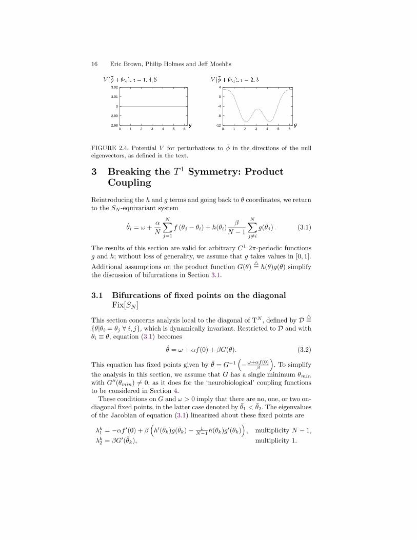
Example 2. Suppose N = 6 and f(·) = sin(·), and consider the ((S3)2oZ2)-

invariant equilibria (e.g., (φ1, φ2, φ3, φ4, φ5, φ6) = (0, 0, 0, π, π, π) ≡ φ).From Proposition 2.7, the eigenvalues for such equilibria are 0 with mul-tiplicity five, and 6α with multiplicity one. The null eigenvectors may betaken to be e1=(1, 1, 1, 1, 1, 1), e2=(2,−1,−1, 0, 0, 0), e3=(1, 1,−2, 0, 0, 0),e4 = (2,−1,−1, 2,−1,−1), e5 = (1, 1,−2, 1, 1,−2). Figure 2.4 shows thepotential V corresponding to perturbations to φ in the directions of thesenull eigenvectors. V is flat for perturbations in the e1, e4, and e5 directions(each with a corresponding one-dimensional continuum of fixed points,overall giving a three-torus of equilibria), but not for perturbations in thee2 and e3 directions. Proposition 2.10 guarantees the existence of the three-torus of equilibria Fix[Z2] given by (φ1, φ2, φ3, φ4, φ5, φ6) = (ξ1, ξ2, ξ3, ξ1 +π, ξ2 + π, ξ3 + π); note that perturbations to φ in the e1, e4, and e5 direc-tions keep the system in the Fix[Z2] subspace. The e2 and e3 perturbationsillustrate that every zero eigenvalue of Propositions 2.7 or 2.8 does not nec-essarily imply a corresponding one-dimensional continuum of fixed points.


2.98

2.99

3

3.01

3.02

0 1 2 3 4 5 6-12

-8

-4

0

4

0 1 2 3 4 5 6

� �

�� "!#�%$

FIGURE 2.4. Potential V for perturbations to φ in the directions of the nulleigenvectors, as defined in the text.

3 Breaking the T 1 Symmetry: ProductCoupling

Reintroducing the h and g terms and going back to θ coordinates, we returnto the SN -equivariant system

θi = ω +α

N

N∑

j=1

f (θj − θi) + h(θi)β

N − 1

N∑

j 6=i

g(θj) . (3.1)

The results of this section are valid for arbitrary C1 2π-periodic functionsg and h; without loss of generality, we assume that g takes values in [0, 1].

Additional assumptions on the product function G(θ)4= h(θ)g(θ) simplify

the discussion of bifurcations in Section 3.1.

3.1 Bifurcations of fixed points on the diagonal

Fix[SN ]

This section concerns analysis local to the diagonal of TN , defined by D4=

{θ|θi = θj ∀ i, j}, which is dynamically invariant. Restricted to D and withθi ≡ θ, equation (3.1) becomes

θ = ω + αf(0) + βG(θ). (3.2)

This equation has fixed points given by θ = G−1(−ω+αf(0)

β

). To simplify

the analysis in this section, we assume that G has a single minimum θminwith G′′(θmin) 6= 0, as it does for the ‘neurobiological’ coupling functionsto be considered in Section 4.

These conditions on G and ω > 0 imply that there are no, one, or two on-diagonal fixed points, in the latter case denoted by θ1 < θ2. The eigenvaluesof the Jacobian of equation (3.1) linearized about these fixed points are

λk1 = −αf ′(0) + β(h′(θk)g(θk)−

1N−1h(θk)g

′(θk)), multiplicity N − 1,

λk2 = βG′(θk), multiplicity 1.


Stability in the transverse directions (with respect to the diagonal) is de-termined by λ1, and in the axial direction by λ2; note that our hypothesison G implies that λ2(θ1) < 0, and λ2(θ2) > 0. As β is decreased throughβ = (ω + αf(0))/|G(θmin)|, the two fixed points coalesce and disappearin a saddle node bifurcation (the appearance of these fixed points as βincreases represents the phenomenon of oscillator death: Ermentrout andKopell [1990]; Taylor and Holmes [1998]). For the remaining values of β,the orbit along D is the (SN symmetric) periodic orbit θD(t). We will in-vestigate the period and stability of this orbit in the following sections.

3.2 Frequency and stability of the in-phase periodic

orbit

If β < (ω + αf(0))/|G(θmin)|, the period of the orbit on D is given by

τ =

∫ 2π

0

(dθ

dt

)−1dθ =

∫ 2π

0

dθ

ω + αf(0) + βh(θ)g(θ). (3.3)

Moreover, we have

3.1 Proposition. (Local stability of D.) The SN -symmetric periodic so-lution θi(t) ≡ θD(t) along D is asymptotically stable if

α >βN

(N − 1)τf ′(0)

∫ 2π

0

g(θ)h′(θ)

ω + αf(0) + βg(θ)h(θ)dθ , (3.4)

where τ is the (generally α-dependent) period of θD(t) given in equation(3.3) and we assume f ′(0) > 0.

Closely related results are found in Tsang, Mirollo, and Strogatz [1991];Golomb, Hansel, Shraiman, and Sompolinsky [1992].

Proof. Linearized around θD(t), equation (3.1) becomes ξi = [Ad(t)ξ]i.The proof uses the fact that the (t-dependent) symmetric matrix Ad(t)has a particularly simple structure, and that it can be diagonalized bya t-independent similarity transformation. Specifically, the eigenvalues ofAd(t), where t is viewed as a (fixed) parameter, are:

λ1(t)=−αf′(0) + β

(g(t)h′(t)−

1

N − 1h(t)g′(t)

), multiplicity N − 1 ,

λ2(t)= βG′(t), multiplicity 1,

where g(t) is written for g(θD(t)), etc. The orthogonal eigenvectors of λ1(t)(denoted by χ1, . . . , χN−1) may be chosen constant and orthogonal to theeigenspace of λ2(t), which is spanned by the eigenvector (1, . . . , 1)T. Thus,


χ1, . . . , χN−1 span the space normal to θD(t). In these eigencoordinates thelinearized system decouples as

ξi = λ1(t)ξi, i = 1, . . . , N − 1, ξN = λ2(t)ξN .

Define the (N −1)-dimensional plane∑

= {χ|χN = 0} and consider thePoincare map P : U → U for some neighborhood U ⊂

∑of 0. The orbit

θD(t) intersects∑

at 0, which is a fixed point for P . For i = 1, . . . , N −1, P : ξi 7→ (exp

∫ τ0λ1(t)dt)ξi so that 0 is a stable fixed point for P if∫ τ

0λ1(t)dt < 0. (Due to the periodicity of G(t),

∫ τ0λ2(t)dt ≡ 0, as it must,

being the Floquet exponent along the periodic orbit). We have

∫ τ

0

λ1(t)dt

=

∫ τ

0

(−αf ′(0) + β

[g(t)h′(t)−

1

N − 1h(t)g′(t)

])dt

= −αf ′(0)τ +

∫ 2π

0

β

(−[h(θ)g′(θ) + h′(θ)g(θ)]

N − 1+Ng(θ)h′(θ)

N − 1

)θ−1dθ

= −αf ′(0)τ −1

N − 1ln[ω + αf(0) + βh(θ)g(θ)]2π0

+

∫ 2π

0

βNg(θ)h′(θ)

(N − 1)(ω + αf(0) + βh(θ)g(θ))dθ (3.5)

= −αf ′(0)τ +

∫ 2π

0

βNg(θ)h′(θ)

(N − 1)(ω + αf(0) + βh(θ)g(θ))dθ , (3.6)

where the second term in equation (3.5) vanishes due to the 2π-periodicityof h and g. Thus,

∫ τ0λ1(t)dt < 0 when the inequality of Proposition 3.1

is satisfied. Since stability of the fixed point 0 under P implies stability ofθD(t) for equation (2.1), the Proposition is proven. ¥

A simple calculation using integration by parts and the 2π-periodicity ofg and h shows that for α = 0 and asymptotically small β, the right-handside of (3.6) becomes βN

N−1f′s(0), which (cf. (2.13)) determines the stability

of the in-phase solution if synaptic coupling βN−1h(θi)

∑j 6=i g(θj) is taken

to be weak and then averaged to yield βN−1

∑j 6=i fs(θj−θi). This agreement

between the averaged and original versions of (3.1) for sufficiently small β isexpected from the averaging theorem (Guckenheimer and Holmes [1983]),and reveals how (3.4) generalizes the stability result found in van Vreeswijk,Abbot, and Ermentrout [1994]; Hansel, Mato, and Meunier [1995] forN = 2and averaged synaptic coupling.

Equation (3.4) may be used to estimate a critical value αloc such that

θD(t) is asymptotically stable for α > αloc. Letting h be a Lipschitz con-


stant for h, we note that

∫ 2π

0

g(θ)h′(θ)

ω + αf(0) + βh(θ)g(θ)dθ ≤

∫ 2π

0

h

ω + αf(0) + βh(θ)g(θ)dθ = hτ,

(3.7)where the inequality follows from the bound on g and the definition of the

Lipschitz constant. Thus, from (3.4) we have stability if α > Nβh(N−1)f ′(0)

4=

αloc. With f(0) = 0 (e.g. if f is odd), this estimate can be refined: theright-hand side of equation (3.4) is independent of α, so that the (smallest)critical value αloc is

αloc =βN

(N − 1)τf ′(0)

∫ 2π

0

g(θ)h′(θ)

ω + βg(θ)h(θ)dθ. (3.8)

We now turn to the nonlinear stability properties of D.

Estimate for the domain of attraction of D

3.2 Proposition. (Nonlinear stability of D.) For some s > 1, assumef ′(0) > 0 and let R > 0 be the smallest value for which either f ′(2R) =f ′(0)/s > 0 or f ′(−2R) = f ′(0)/s > 0 (implying minθ∈[−2R,2R] f

′(θ) =

f ′(0)/s). Let G be the Lipschitz constant for G(·) = g(·)h(·), and define

h1(θi) = maxθ{|h′(θi)g(θ)| : |θi− θ| < 2R} and h1 = maxθi

{h1(θi)}. Then,for

α > αglob4=sβ(Nh1 + G)

(N − 1)f ′(0), (3.9)

the domain of attraction for D includes CR4= {θ|d(θ, θd(ψ)) ≤ R for some

ψ ∈ [0, 2π]} (cf. Figure 2.2).

Proof. Fix an arbitrary ψ ∈ [0, 2π). Consider the (non-orthogonal) basisb ≡ {xi|i = 1, . . . , N − 1}, where xi ≡ θi − θi+1. We define Xψ, the N − 1dimensional space perpendicular to the axis of CR at θd(ψ), as the copy ofspan b containing θd(ψ). In other words, Xψ is the normal space N (θd(ψ)).

Now, define the squared ‘radius’ R =∑N−1i=0 x2i . We will show that R =

2∑N−1i=0 xixi ≤ 0 for all x ∈ CR. The cylindrical surfaces {x|R(x) = c} will

therefore be crossed ‘inward’ toward the axis of CR.Take an arbitrary θ ∈ CR ∩Xψ. For such a θ, we also have θ ∈ BR(ψ) =

{θ|d(θ, θd(ψ)) < R}. Thus |θj − θi| < 2R ∀ i, j (and, in particular, |xi| <


2R ∀ i). These inequalities allow us to find a bound on each xi:

xi = ˙θi − θi+1

=α

N

N∑

j=1

f(θj − θi)−α

N

N∑

j=1

f(θj − θi+1)

+β

N − 1h(θi)

N∑

j 6=i

g(θj)−β

N − 1h(θi+1)

N∑

j 6=i+1

g(θj)

=α

N

N∑

j=1

[f(θj − θi)− f(θj − θi + xi)] +β[h(θi)− h(θi+1)]

N − 1

N∑

j=1

g(θj)

+β[h(θi+1)g(θi+1)− h(θi)g(θi)]

N − 1. (3.10)

xi< −α[f ′(0)/s]xi + β N

N−1 h1xi +β

N−1 Gxi4= kxi if xi > 0

> −α[f ′(0)/s]xi + β NN−1 h1xi +

βN−1 Gxi

4= kxi if xi < 0

}. (3.11)

The inequalities (3.11) use the hypothesis on f ′, the bound g(θ) ≤ 1,

and the definitions of h and G. Thus, for k < 0 (i.e. α > αglob), R =

2∑N−1i=0 xixi < 0 unless xi = 0, ∀i. This argument may be repeated for

any ψ and therefore for any arbitrary θ ∈ CR, so the Proposition follows. ¥

Since nonlinear stability implies local stability, it must follow from α >αglob that inequality (3.4) is satisfied. This may be seen from the fact thatα > αglob implies α > αloc and comparing equation (3.9) with (3.7).

Finally, we note that Proposition 3.2 may be sharpened by refining the es-timates in (3.11) in any manner that also implies sign(xi) = −sign(xi). For

example, a lower value h2 can replace h1 above, where h2 = maxθih2(θi)

and h2(θi) = maxθ{h′(θi)g(θ) : |θi− θ| < 2R} (note that although we have

dropped the absolute value in the maxθ, h2 ≥ 0 since h is periodic). The

bound h2 arises as follows. If the second term in (3.10) is of opposite sign toxi, it favors the conclusion sign(xi) = −sign(xi) and hence may be ignoredfor the purposes of bounding α such that k < 0. Thus the natural questionis: assuming that it is of the same sign as xi, can we find a smaller upperbound than β N

N−1 h1xi on the magnitude of this second term? The answeris yes: since [h(θi) − h(θi+1)] = [h(xi + θi+1) − h(θi+1)], this difference

cannot exceed the upper bound β NN−1 h2xi, as desired.


4 Application to a model of the locus

coeruleus

Here we apply the analysis above to a model of the locus coeruleus brainnucleus. First, we introduce specific coupling functions f , g, and h appro-priate to neuronal coupling.

4.1 Coupling functions

The functions f and g, h, corresponding to electrotonic and synaptic cou-pling, were computed using both the strong attraction (SA) and phase re-sponse (PR) methods mentioned in the introduction. The Hodgkin-Huxley(HH) equations with input current 10 µA/cm2 were used (Hodgkin andHuxley [1952]). In their original form these equations were derived fromthe giant axon of a squid, so their use here merely represents a proof ofconcept. Reduction of more realistic mammalian neuron models, which in-clude calcium-dependent potassium channels and whose action potentialspikes occupy a much smaller fraction of the period than in the rescaledHH equations, is in progress (Brown, Moehlis, Holmes, Aston-Jones, andClayton [2002]), and leads to coupling functions somewhat different fromthose considered here, although the general structure of the phase equationssurvives.

The effect of electrotonic coupling on the time derivative Vi of neuron i’svoltage was taken to be α

N

∑Nj=1(Vj−Vi) (cf. Johnston and Wu [1997]), and

the inhibitory synaptic effect to be (EK−Vi)β

N−1

∑j 6=iA(Vj , t), where EK

is the reversal potential for potassium and A(Vj , t) is an ‘alpha function’

which takes values in [0, A], A < 1, and represents the influence of neuron jon post-synaptic cells. Specifically, A(Vj , t) = ((t− tjs− td)/τA) · exp(−(t−tjs − td)/τA), where t

js is the time at which the voltage of neuron j spikes

(see below), td is the synaptic delay, and τA is the synaptic time constant(e.g. Kim and Lee [2000]). The effective value of τA for LC neurons has beenobserved to be much longer than those of typical synaptic connections dueto the slow dynamics of norepinephrine neurotransmitter uptake (Grant,Aston-Jones, and Redmond [1988]; Aston-Jones, Rajkowski, and Alexinsky[1994]). We parameterize the limit cycle of the uncoupled HH equations bya time scaled so that the period T = 2π

ωis 1/3 sec (to match our estimate

for LC neurons), and take τA = 0.025 sec and td = 0.150 sec. These neuronand coupling models and parameters lead to the reductions of the couplingfunctions to TN displayed in Figure 4.1.

Under the idealisation that neurons in the small LC nucleus are identical(Williams, North, Shefner, Nishi, and Egan [1984]) and globally coupled,our LC model simplifies to equation (1.2). As coupling becomes stronger,modifications to f , g, and h may be required to maintain the accuracy ofphase reductions; for the purpose of this paper, these effects are neglected.


0 2 4 6

5

10

15

0 2 4 6−3−2−1

01

0 2 4 6−5

0

5

0 2 4 6

−50

0

50

0 2 4 6

−6−4−2

0

0 2 4 60

50

100

�

�

�

��

��

��

�

�

�

��

� ��

� ��

FIGURE 4.1. Coupling functions derived from the (time-reparameterized)Hodgkin-Huxley equations. The subscript e (s) refers to electrotonic (synaptic)coupling, while the superscript PR (SA) indicates that the function was derivedusing the phase reduction (strong attraction) method. The h’s and g are calcu-lated for the synaptic coupling described in the text: fPR

s is obtained by averagingthe product of g and hPR, and fPR

e is obtained by averaging the electrotonic cou-pling using a phase response method (cf. Kim and Lee [2000]). fSAe is obtainedby first assuming that the limit cycle is infinitely attracting, followed by averag-ing (cf. Ermentrout and Kopell [1990]; Hoppensteadt and Izhikevich [1997]). The‘spikes’ in hSA(θ) are associated with the projection of coupling functions nearturning points in the original phase variables; the tips extend to approximately±30 (there is also an O(1) spike near θ = 0, not visible here).

However, Brown, Moehlis, Holmes, Aston-Jones, and Clayton [2002] in-cludes a careful comparison of phase-reduced and ‘full’ conductance-basedLC models in the relevant parameter range.

4.2 Modeling synchrony in LC modes

This section demonstrates that cross correlograms qualitatively similar tothose of Figure 1.1(a) can arise in our phase-reduced LC model due toincreased coupling in the phasic LC mode relative to the tonic mode.

Cross correlograms are derived from solutions of (3.1) as follows. A spikeis deemed to occur when a rotator θi crosses through a threshold valueθs: the solution of {V (θs) = Vs, V

′(θs) > 0}, where Vs = −30mV is adepolarized voltage characteristic of a neuron firing an action potentialand the function V (θ) is defined by V (t) = V (θ/ω) over the period of oneneuron action potential. The set of all pairwise differences between times atwhich distinct spike events occur is computed according to this definition,and the cross correlogram is the histogram of this set.


PR PR PR PR SAκ = 0 κ = 10 κ = 50 κ = 100 κ = 0

(Sk)m o Zm

S, m = 1,2,4 1,2,4 1,4 1 1,3,4

U, m = 3,6,8,12 3,6,8,12 2,3,6,8,12 2,3,4,6,8,12 2,6,8,12

SN−p × Sp

S, p = 11,12 12 1,2 1-4 1-6

U, p = 1-12 1-12 1-12 3-12 7-12

TABLE 1.1. The linear stability of various ‘clustered’ periodic orbits of diagonalflow for different phase difference couplings fe(θji) + κfs(θji), computed usingthe PR or SA methods. (Sk)

m o Zm stability is given for allowable m (N = 24),and SN−p × Sp stability for N = 24 and p = 1, ..., 12; a value of p being listedtwice indicates the correspondence of multiple δ’s. S and U indicate asymptoticstability and instability, respectively, for them or p values given in the subsequentcolumns.

Phase-difference coupling

In this section we assume that synaptic coupling βN−1h(θi)

∑j 6=i g(θj) is

sufficiently weak that it can be averaged to yield βN−1

∑j 6=i fs(θj − θi),

and we take β = κα, so that (3.1) becomes θi = ω + αN

∑j f(θji), where

the phase difference function f(·) = fe(·) + κfs(·). We use the methods ofSection 2 to determine stability of periodic orbits. The results are shownin Table 1.1 for various values of κ and coupling functions derived with thePR and SA methods. The SA coupling functions give rise to a larger set ofdistinct stable periodic orbits, the consequences of which will be discussedbelow.

To model the phasic and tonic behavior of Figure 1.1, we consider equa-tion (2.1) in the presence of noise represented as additive Brownian forcingon the torus, so that:

dθi =

ω +

α

N

n∑

j 6=i

f (θj − θi)

dt+ σdW i

t . (4.1)

The inclusion of random noise represents additional inputs currents to LCneurons, a common stratagem in accounting for the influence of neuralsubgroups neglected in the model. The stochastic averaging theorem (Zhu[1988]; Freidlin and Wentzell [1998]) leads to the approximation above,including σ being independent of θ; in particular, σ2 = z2γ, where γis the variance of Brownian input currents, z(θ) is the phase responsecurve (PRC, cf. Kuramoto [1997]), and the overbar denotes the average

(·) = 12π

∫ 2π

0(·)dθ. Simulations of equation (4.1) to be discussed below were

performed using a second order stochastic Runge-Kutta method (Honey-cutt [1992]).


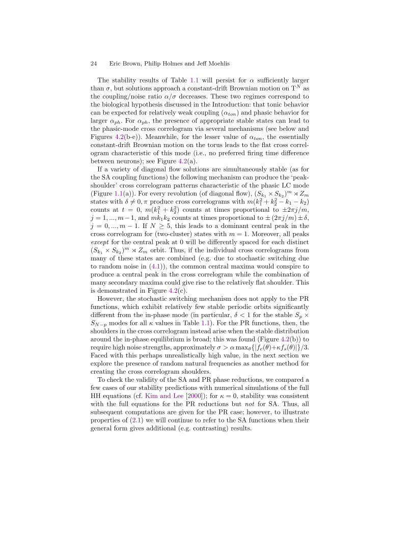
The stability results of Table 1.1 will persist for α sufficiently largerthan σ, but solutions approach a constant-drift Brownian motion on TN asthe coupling/noise ratio α/σ decreases. These two regimes correspond tothe biological hypothesis discussed in the Introduction: that tonic behaviorcan be expected for relatively weak coupling (αton) and phasic behavior forlarger αph. For αph, the presence of appropriate stable states can lead tothe phasic-mode cross correlogram via several mechanisms (see below andFigures 4.2(b-e)). Meanwhile, for the lesser value of αton, the essentiallyconstant-drift Brownian motion on the torus leads to the flat cross correl-ogram characteristic of this mode (i.e., no preferred firing time differencebetween neurons); see Figure 4.2(a).

If a variety of diagonal flow solutions are simultaneously stable (as forthe SA coupling functions) the following mechanism can produce the ‘peak-shoulder’ cross correlogram patterns characteristic of the phasic LC mode(Figure 1.1(a)). For every revolution (of diagonal flow), (Sk1 ×Sk2)

moZmstates with δ 6= 0, π produce cross correlograms with m(k21 + k22 − k1 − k2)counts at t = 0, m(k21 + k22) counts at times proportional to ±2πj/m,j = 1, ...,m−1, and mk1k2 counts at times proportional to ± (2πj/m)± δ,j = 0, ...,m − 1. If N ≥ 5, this leads to a dominant central peak in thecross correlogram for (two-cluster) states with m = 1. Moreover, all peaksexcept for the central peak at 0 will be differently spaced for each distinct(Sk1 × Sk2)

m o Zm orbit. Thus, if the individual cross correlograms frommany of these states are combined (e.g. due to stochastic switching dueto random noise in (4.1)), the common central maxima would conspire toproduce a central peak in the cross correlogram while the combination ofmany secondary maxima could give rise to the relatively flat shoulder. Thisis demonstrated in Figure 4.2(c).

However, the stochastic switching mechanism does not apply to the PRfunctions, which exhibit relatively few stable periodic orbits significantlydifferent from the in-phase mode (in particular, δ < 1 for the stable Sp ×SN−p modes for all κ values in Table 1.1). For the PR functions, then, theshoulders in the cross correlogram instead arise when the stable distributionaround the in-phase equilibrium is broad; this was found (Figure 4.2(b)) torequire high noise strengths, approximately σ > αmaxθ{|fe(θ)+κfs(θ)|}/3.Faced with this perhaps unrealistically high value, in the next section weexplore the presence of random natural frequencies as another method forcreating the cross correlogram shoulders.

To check the validity of the SA and PR phase reductions, we compared afew cases of our stability predictions with numerical simulations of the fullHH equations (cf. Kim and Lee [2000]); for κ = 0, stability was consistentwith the full equations for the PR reductions but not for SA. Thus, allsubsequent computations are given for the PR case; however, to illustrateproperties of (2.1) we will continue to refer to the SA functions when theirgeneral form gives additional (e.g. contrasting) results.


−0.2 0 0.20

2

4

6

x 104

−0.2 0 0.20

2

4

6

x 104

−0.2 0 0.20

2

4

6

x 104

−0.2 0 0.20

2

4

6

x 104

−0.2 0 0.20

2

4

6

x 104

a) b) c) d) e)

��

��

��

��

��

��

FIGURE 4.2. Cross correlograms for simulations of the tonic ‘low-coupling’ (a)and phasic ‘high-coupling’ (b-e) LC modes using the phase-difference model (4.1).To facilitate comparison, αph was chosen so that αph maxθ{|f(θ)|} = 2.25 for boththe SA and PR coupling functions; also, αton = αph/5, ω = 6π, and N = 24. (a)PR model with κ = 0, σ = 0.8, and α = αton; (b) same except with α = αph;(c) SA model with κ = 0 and σ = 0.2, α = αph. (d) As described in Section 4.2,phasic PR simulation as in (a) but with randomly distributed frequencies (drawnfrom the Cauchy distribution with parameter 0.2 and mean ω) and σ = 0.1.(e) as in (b), but with the addition of phase-dependent (synaptic) coupling ofstrength β = 0.23. The range of all histograms is [−.7τ, .7τ ], where τ = 1/3 secis the simulated natural period; all histograms are averaged over five simulatedrecordings with uniformly distributed initial conditions, with each trial 2 min induration.

Breaking the SN symmetry with random natural frequencies

By the standard theorems for normally hyperbolic invariant manifoldsFenichel [1971]; Wiggins [1994], many of our stability results persist un-der small perturbations from fully SN × T 1- or SN -equivariant systems.To study these effects, we performed numerical simulations: in particu-lar, we considered the phase-difference system (4.1) with randomly dis-tributed frequencies ω → ωi (so that the noise-free system has no nontriv-ial isotropy subgroups). This is appropriate because individual LC neuronsexhibit a range of natural frequencies Grant, Aston-Jones, and Redmond[1988]; Aston-Jones, Rajkowski, and Alexinsky [1994]. In Figure 4.2(d), weshow a reproduction of the phasic mode cross correlogram for the averagedPR coupling function with κ = 0 and frequencies randomly distributedaround ω with a Cauchy distribution with parameter 0.2. This correspondsto a tight distribution; nevertheless, the relatively low noise value σ = 0.1is sufficient to reproduce patterns similar to those in Figure 1.1.

We note that there are some analytical results (e.g. Kuramoto [1984];Strogatz [2000]; Crawford [1995]; Crawford and Davies [1999]) for the dis-tributed frequency, phase-difference system as N →∞. However, a finite-Nanalysis of the full equation (2.1) with distributed phases and phase prod-uct coupling term remains open, to the best of our knowledge.


Phase-dependent coupling

We now return to consider equation (3.1) with unaveraged synaptic (prod-uct) coupling. Since f(0) = 0 for electrotonic coupling, we may use equa-tion (3.8) to explicitly calculate a lower bound on α for this orbit to bestable. The resulting αloc < 0 (Figure 4.3), so that the in-phase state isstable for synaptic coupling and any positive α (since f ′(0) > 0). In ad-dition, the domain of attraction may be estimated: for example, takings = 2.14 in Proposition 3.2 gives R = 1/4 and h2 = 28.1 for PR couplingfunctions with κ = 0. Thus, the domain of attraction of the in-phase orbitincludes CR if α > αglob = 7.11β (equation (3.9) for N →∞). Figure 4.2(e)demonstrates the collapse of the cross correlogram (d) upon addition of thesynchronizing (cf. Section 4.2) product coupling.

For the SA coupling functions, the following observation is useful: sincethe denominator in the integrand of (3.4) is always positive, if h′(θ) < 0 forθ in the (essential) support of the positive function g then the integranditself will always be negative, giving stability for any α > 0. The plots inFigure 4.1 show that for delays td (which correspond to translations of g)taken in a wide range around 0.150 sec, stability holds for arbitrary g ofreasonably compact essential support and any α, β > 0 such that the in-phase periodic orbit exists. We note here that related stability conditionsare derived in van Vreeswijk, Abbot, and Ermentrout [1994]; Ermentrout[1996]; Gerstner, van Hemmen, and Cowan [1996], in which the time courseof g is also important.

4.3 Modeling firing rates in LC modes

Here we show that the depressed firing rates characteristic of the pha-sic mode can be captured by our LC model if explicitly phase-dependentsynaptic terms are included.

Phase-difference coupling

Under the assumption that the period of the in-phase state largely deter-mines average LC firing rates, the depressed firing rate observed in thephasic mode cannot be reproduced with averaged (phase-difference), PRcoupling functions. The period of the in-phase state of (4.1) is 2π

ω+αf(0) ,

and Figure 4.1 shows that f(0) > 0 for any κ > 0, so that the period willalways decrease as α increases. Hence, the (highly-coupled) phasic statewould actually have an increased firing rate. In contrast, we shall see that(3.1) allows us to correctly reproduce observed firing rates.

Phase-dependent coupling

For small β, where averaging is valid, the period of the SN symmetricorbit must decrease with β. However, Figure 4.3 also shows that for β


sufficiently large, the period increases with β (the term G(θ) in (3.2) slowsthe flow). Since the SN symmetric orbit is attracting, its increasing periodindicates a mechanism for lower firing rates in the phasic mode. This showsthe importance in this case of considering the explicit product couplingof (3.1); however, for other parameter values and neuron models phase-difference coupling may correctly capture trends in firing rates (cf. Brown,Moehlis, Holmes, Aston-Jones, and Clayton [2002]).

0 0.5 1 1.5 2−1

−0.5

0

0 0.5 1 1.5 20.32

0.34

0.36

0.38

0.4

0.42

� �

��

FIGURE 4.3. The β-dependence of (left) bounds for stability and (right) the pe-riod of the SN symmetric orbit with PR coupling functions, from equations (3.8)and (3.3) in the large-N limit.

4.4 LC response to stimulus

Figures 1.1(b,c) show averaged histograms of the times at which spikeswere recorded in LC neurons, in data accumulated from many stimulus-response trials. The phasic histogram displays a post-stimulus window inwhich the probability of a given LC neuron firing in an arbitrary trial isrelatively high; this represents increased activity following stimulus. Afterthis burst the histogram exhibits a ‘refractory’ period in which there is alower firing probability, followed by a gradual return to equilibrium firingprobability. We now indicate a mechanism by which this pattern can emergefrom averages over many trials of oscillator dynamics with the appropriateinitial conditions.

As noted in the Introduction, the LC response in the phasic mode isstronger than in the tonic mode. This effect can be shown to arise fromthe fact that phasic-mode LC neurons tend to have lower firing frequen-cies (Brown, Moehlis, Holmes, Aston-Jones, and Clayton [2002]). Here weonly study phase-difference models based on equation (4.1) for the phasic-mode LC response. We assume that external stimuli act (via other neuralgroups) by increasing the input current to each LC neuron identically viaa function I(t), contributing a term z(θ)I(t) to the phase velocities. Ap-proximating the phasic mode as perfectly synchronized so that the averageαN

∑nj 6=i f (θj − θi) may be replaced by the constant f(0), equation (4.1)

becomes

dθ = [ω + αf(0) + z(θ)I(t)] dt+ σdWt4= v(θ, t)dt+ σdWt . (4.2)


Initial conditions θ(0) = θ0 are drawn from the appropriate distribution(see below).

The probability density of oscillator phases for this stochastic ODE (4.2)evolves according to the forward Kolmogorov equation

∂ρ(θ, t)

∂t= −

∂

∂θ[v(θ, t)ρ(θ, t)] +

σ2

2

∂2ρ(θ, t)

∂θ2, (4.3)

with ρ(θ, t = 0) = δ(θ − θ0). Due to the linearity of (4.3), histogramsto be compared with Figure 1.1 may be produced from (4.3) with initialdensity representing an average over many trials, in which case ρ(θ, t)dθrepresents the probability that a given neuron observed in an arbitrarytrial has phase in the interval [θ, θ+ dθ) at time t. This ‘density’ approachto modeling experimental firing time histograms is also employed in Rittand Kopell [2002]. The experimentally relevant initial condition ρ0 may befound by reasoning as follows: if v lacks explicit t-dependence (i.e. I(t) = 0),then the probability that an oscillator obeying (4.2) is in [θ, θ+ dθ] shouldscale with 1/T (θ), where T (θ) is the time spent in this interval during onecycle. To lowest order in dθ and neglecting noise, this implies ρ(θ, t = 0) =C/v(θ) for some constant C; normalization gives ρ0 itself, which is simply1/2π in this case. Histograms of firing times may be extracted from thesolutions of (4.3) by noting that the firing probability (for an arbitrarilychosen neuron) at time t is proportional to the threshold probability flux

FL(t)4= v(θs, t)ρ(θs, t).

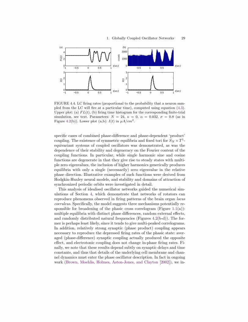
We can develop explicit solutions to (4.3) for certain classes of stimuliand PRCs in the absence of noise for comparison with experimental data;these analyses will appear in a future paper (Brown, Moehlis, Holmes,Aston-Jones, and Clayton [2002]). Figure 4.4 illustrates preliminary resultsrelevant to the data of Figure 1.1(b,c) via numerical solutions of (4.3) anddirect simulations of (4.1) (with identical stimuli), which show that FL(t),derived from (4.3), provides a reasonable approximation for post-stimulusfiring probabilities. We note that FL(t) displays the characteristic peak andrefractory period of Figures 1.1(b,c), but the subsequent return to equilib-rium is slow and exhibits prolonged ‘ringing’ not seen in the experimentaldata. The ringing is due to a ‘resonance’ between the stimulus durationand the oscillator frequency; it is diminished or disappears entirely, givinghistograms more similar to Figures 1.1(b,c), when data is averaged overa distribution of frequencies (Brown, Moehlis, Holmes, Aston-Jones, andClayton [2002]).

5 Conclusions

The dynamics of a finite set of identically (mean field) coupled oscilla-tors were analyzed in general cases of phase-difference coupling and in


−1 −0.5 0 0.5 10

2

4

−1 −0.5 0 0.5 10

1

2

3

−0.5 1 0.50

1000

2000

−1 −0.5 0 0.5 10

1

2

3

(a) (b)

coun

ts

FL

(t)

t(sec)

t(sec)t(sec)

t(sec)

I(t)

I(t)

FIGURE 4.4. LC firing rates (proportional to the probability that a neuron sam-pled from the LC will fire at a particular time), computed using equation (4.3).Upper plot: (a) FL(t), (b) firing time histogram for the corresponding finite-trialsimulation, see text. Parameters: N = 24, κ = 0, α = 0.032, σ = 0.8 (as inFigure 4.2(b)). Lower plot (a,b): I(t) in µA/cm2.

specific cases of combined phase-difference and phase-dependent ‘product’coupling. The existence of symmetric equilibria and fixed tori for SN ×T

1-equivariant systems of coupled oscillators was demonstrated, as was thedependence of their stability and degeneracy on the Fourier content of thecoupling functions. In particular, while single harmonic sine and cosinefunctions are degenerate in that they give rise to steady states with multi-ple zero eigenvalues, the inclusion of higher harmonics generically producesequilibria with only a single (necessarily) zero eigenvalue in the relativephase direction. Illustrative examples of such functions were derived fromHodgkin-Huxley neural models, and stability and domains of attraction ofsynchronized periodic orbits were investigated in detail.

This analysis of idealised oscillator networks guided the numerical sim-ulations of Section 4, which demonstrate that networks of rotators canreproduce phenomena observed in firing patterns of the brain organ locuscoeruleus. Specifically, the model suggests three mechanisms potentially re-sponsible for broadening of the phasic cross correlogram (Figure 1.1(a)):multiple equilibria with distinct phase differences, random external effects,and randomly distributed natural frequencies (Figures 4.2(b-d)). The for-mer is perhaps least likely, since it tends to give multi-peaked correlograms.In addition, relatively strong synaptic (phase product) coupling appearsnecessary to reproduce the depressed firing rates of the phasic state: aver-aged (phase-difference) synaptic coupling actually produced the oppositeeffect, and electrotonic coupling does not change in-phase firing rates. Fi-nally, we note that these results depend subtly on synaptic delays and timeconstants, and thus that details of the underlying cell membrane and chan-nel dynamics must enter the phase oscillator description. In fact in ongoingwork (Brown, Moehlis, Holmes, Aston-Jones, and Clayton [2002]), we in-


corporate an additional slow calcium-dependent potassium current, leadingto coupling functions differing from those of Figure 4.1, and, in some cases,remarkably close to the degenerate pure sinusoids.

A general point of contact between the present study and neurosciencelies in the relationship between explicitly modeling individual neurons andtheir couplings, and averaging the behavior of a (sub-)population into asingle connectionist-type ‘unit’ (e.g. Rumelhart and McClelland [1986]).Domain of attraction and probability density results for synchronized statesmay inform conditions under which such approximations are justifiable.In the present paper, a simple probabilistic evolution (equation (4.3)) forcoherent phase states produces acceptable results (Figure 4.4). Extensionof this result to a true population average for systems with distributedfrequencies and non-uniform couplings would bring it closer to the work ofSirovich, Knight, and Omurtag [2000], and help unify detailed (Hodgkin-Huxley type) neural models, simpler integrate-and-fire and phase models,and connectionist networks.

Acknowledgments: This work was partially supported by DoE: DE-FG02-95ER25238 and NIMH: MH62196 (Cognitive and Neural Mecha-nisms of Conflict and Control, Silvio M. Conte Center). Eric Brown wassupported by a National Science Foundation Graduate Fellowship and aBurroughs-Wellcome Training Grant in Biological Dynamics: 1001782, andJeff Moehlis by a National Science Foundation Postdoctoral Research Fel-lowship. We thank Jason Ritt for assistance with incorporating the stim-ulus into the density approach as well as other helpful comments, GeorgiMedvedev for useful suggestions and discussions, and Martin Golubitsky foran insightful and stimulating communication early in this project. WeinanE provided motivation for studying and insights about symmetric solutionsin the N →∞ limit.

This is page 31Printer: Opaque this

Bibliography

Arnold, V. [1973], Ordinary Differential Equations. MIT Press, Boston.

Ashwin, P. and J. Swift [1992], The dynamics of N weakly coupled identicaloscillators, J. Nonlin. Sci. 2, 69–108.

Aston-Jones, G., J. Rajkowski, and T. Alexinsky [1994], Locus coeruleusneurons in the monkey are selectively activated by attended stimuli in avigilance task., J. Neurosci. 14, 4467–4480.

Bressloff, P. and S. Coombes [1998], Spike train dynamics underlying pat-tern formation in integrate-and-fire oscillator networks, Phys. Rev. Lett.81, 2384–2387.

Brown, E., J. Moehlis, P. Holmes, G. Aston-Jones, and E. Clayton [2002],The influence of spike rate on response in locus coeruleus, Unpub-lished manuscript, Program in Applied and Computational Mathematics,Princeton University, 2002.

Chow, C. and N. Kopell [2000], Dynamics of spiking neurons with electro-tonic coupling, Neural Comp. 12, 1643–1678.

Crawford, J. [1995], Scaling and singularities in the entrainment of globallycoupled oscillators, Phys. Rev. Lett. 74, 4341–4344.

Crawford, J. and K. Davies [1999], Synchronization of globally coupledphase oscillators: singularities and scaling for general couplings, PhysicaD 125 (1-2), 1–46.

Daido, H. [1994], Generic scaling at the onset of macroscopic mutual en-trainment in limit cycles with uniform all-to-all coupling, Phys. Rev. Lett.73(5), 760–763.

E, W. [2001], personal communication, 2001.

Ermentrout, B. [1996], Type I membranes, phase resetting curves, and syn-chrony, Neural Comp. 8, 979–1001.

Ermentrout, G. and N. Kopell [1990], Oscillator death in systems of coupledneural oscillators, SIAM J. on Appl. Math. 50, 125–146.


Fenichel, N. [1971], Persistence and smoothness of invariant manifolds forflows, Ind. Univ. Math. J. 21, 193–225.

Freidlin, M. and A. Wentzell [1998], Random perturbations of dynamicalsystems. Springer, New York.

Gerstner, W., L. van Hemmen, and J. Cowan [1996], What matters inneuronal locking?, Neural Comp. 8, 1653–1676.

Golomb, D., D. Hansel, B. Shraiman, and H. Sompolinsky [1992], Cluster-ing in globally coupled phase oscillators, Phys. Rev. A 45(6), 3516–3530.

Golubitsky, M., I. Stewart, and D. Schaeffer [1988], Singularities andGroups in Bifurcation Theory, Vol. 2. Springer, New York.

Grant, S., G. Aston-Jones, and D. Redmond [1988], Responses of primatelocus coeruleus neurons to simple and complex sensory stimuli., BrainRes. Bull. 21 (3), 401–410.

Guckenheimer, J. and P. Holmes [1983], Nonlinear Oscillations, DynamicalSystems and Bifurcations of Vector Fields. Springer-Verlag, New York.

Hansel, D., G. Mato, and C. Meunier [1995], Synchrony in excitatory neuralnetworks, Neural Comp. 7, 307–337.

Hodgkin, A. and A. Huxley [1952], A quantitative description of membranecurrent and its application to conduction and excitation in nerve, J.Physiol. 117, 500–544.

Honeycutt, R. [1992], Stochastic Runge-Kutta Algorithms I. White Noise,Phys. Rev. A 45, 600–603.

Hoppensteadt, F. and E. Izhikevich [1997], Weakly Connected Neural Net-works. Springer-Verlag, New York.

Izhikevich, E. [2000], Phase equations for relaxation oscillators, SIAM J.on Appl. Math. 60, 1789–1804.

Johnston, D. and S. Wu [1997], Foundations of Cellular Neurophysiology.MIT Press, Cambridge, MA.

Keener, J. and J. Sneyd [1998], Mathematical Physiology. Springer, NewYork.

Kim, S. and S. Lee [2000], Phase dynamics in the biological neural networks,Physica D 288, 380–396.

Kopell, N. and G. Ermentrout [1990], Phase transitions and other phe-nomena in chains of coupled oscillators, SIAM J. on Appl. Math. 50,1014–1052.


Kopell, N. and G. Ermentrout [1994], Inhibition-produced patterning inchains of coupled nonlinear oscillators, SIAM J. Appl. Math. 54, 478–507.

Kopell, N., G. Ermentrout, and T. Williams [1991], On chains of osciallatorsforced at one end, SIAM J. on Appl. Math. 51, 1397–1417.

Kuramoto, Y. [1984], Chemical Oscillations, Waves, and Turbulence.Springer, Berlin.

Kuramoto, Y. [1997], Phase- and center-manifold reductions for large pop-ulations of coupled oscillators with application to non-locally coupledsystems, Int. J. Bif. Chaos 7, 789–805.

Murray, J. [2001], Mathematical Biology, 3rd. Ed. Springer, New York.

Nichols, S. and K. Wiesenfeld [1992], Ubiquitous neutral stability of splaystates, Phys. Rev. A 45(12), 8430–8435.

Okuda, K. [1993], Variety and generality of clustering in globally coupledoscillators, Physica D 63, 424–436.

Ritt, J. and N. Kopell [2002], In preparation, 2002.

Rumelhart, D. and J. McClelland [1986], Parallel Distributed Processing:Explorations in the Microstructure of Cognition. MIT Press, Cambridge,MA.

Servan-Schreiber, D., H. Printz, and J. Cohen [1990], A network model ofcatecholamine effects: Gain, signal-to-noise ratio, and behavior, Science249, 892–895.

Sirovich, L., B. Knight, and A. Omurtag [2000], Dynamics of neuronal pop-ulations: The equilibrium solution, SIAM J. on Appl. Math. 60, 2009–2028.

Strogatz, S. [2000], From Kuramoto to Crawford: Exploring the onset ofsynchronization in populations of coupled oscillators, Physica D 143,1–20.

Taylor, D. and P. Holmes [1998], Simple models for excitable and oscillatoryneural networks, J. Math. Biol. 37, 419–446.

Tsang, K., R. Mirollo, and S. Strogatz [1991], Dynamics of a globally cou-pled oscillator array, Physica D 48, 102–112.

Usher, M., J. Cohen, D. Servan-Schreiber, J. Rajkowski, and G. Aston-Jones [1999], The role of locus coeruleus in the regulation of cognitiveperformance, Science 283, 549–554.


van Vreeswijk, C., L. Abbot, and B. Ermentrout [1994], When inhibitionnot excitation synchronizes neural firing, J. Comp. Neurosci. 1, 313–321.

Watanabe, S. and S. Strogatz [1994], Constants of the motion for super-conducting Josephson arrays, Physica D 74, 195–253.

Watanabe, S. and J. Swift [1997], Stability of periodic solutions in seriesarrays of Josephson Junctions with internal capacitance, J. Nonlin. Sci.7, 503–536.

Wiesenfeld, K., P. Colet, and S. Strogatz [1998], Frequency locking inJosephson arrays: Connection with the Kuramoto model, Phys. Rev. E57 (2), 1563–1569.

Wiggins, S. [1994], Normally Hyperbolic Invariant Manifolds in DynamicalSystems. Springer, New York.

Williams, J., R. North, A. Shefner, S. Nishi, and T. Egan [1984], Membraneproperties of rat locus coeruleus neurons, Neuroscience 13, 137–156.

Zhu, W. [1988], Stochastic averaging methods in random vibration, Appl.Mech. Rev. 41, 189–199.

globally coupled oscillator networks

Documents