government intervention and strategic trading in the u.s
TRANSCRIPT

JOURNAL OF FINANCIAL AND QUANTITATIVE ANALYSIS Vol. 55, No. 1, Feb. 2020, pp. 117–157COPYRIGHT 2018, MICHAEL G. FOSTER SCHOOL OF BUSINESS, UNIVERSITY OF WASHINGTON, SEATTLE, WA 98195doi:10.1017/S0022109018001552
Government Intervention and Strategic Tradingin the U.S. Treasury Market
Paolo Pasquariello, Jennifer Roush, and Clara Vega*
AbstractWe study the impact of permanent open market operations (POMOs) by the Federal Re-serve on U.S. Treasury market liquidity. Using a parsimonious model of speculative trad-ing, we conjecture that i) this form of government intervention improves market liquidity,contrary to conclusions drawn by existing literature; and ii) the extent of this improve-ment depends on the market’s information environment. Evidence from a novel sampleof Federal Reserve POMOs during the 2000s indicates that bid–ask spreads of on-the-runTreasury securities decline when POMOs are executed, by an amount increasing in prox-ies for information heterogeneity among speculators, fundamental volatility, and POMOpolicy uncertainty, consistent with our model.
I. IntroductionDuring the recent financial crisis, several central banks (e.g., the Federal
Reserve, the Bank of England, and the European Central Bank) traded largeamounts of securities. While the motives and effectiveness of these trades con-tinue to be intensely debated (e.g., see Acharya and Richardson (2009)), theirpotential externalities on the “quality” of the process of price formation have re-ceived much less attention.
In this article, we investigate, both theoretically and empirically, the effectsof direct government intervention in a financial market (like central bank trades of
*Pasquariello (corresponding author), [email protected], University of Michigan Ross Schoolof Business; Roush, [email protected]; and Vega, [email protected], Federal Reserve Boardof Governors. We thank Michael Gulick for outstanding research assistance, and an anonymous ref-eree, Gara Afonso, Hendrik Bessembinder (the editor), Sugato Bhattacharyya, Tarun Chordia, RobertEngle, Andreas Fischer, Michael Fleming, Thierry Foucault, Larry Harris, Kentaro Iwatsubo, CollinJones, Andrew Karolyi, Marc Lipson, Anna Obizhaeva, Maureen O’Hara, Amiyatosh Purnanandam,Marti Subrahmanyam, Rufei Zhu, and seminar participants at the Banque de France, University ofWarwick, Swiss National Bank, University College London, the 2011 EFA meetings, the 2011 NBERMarket Microstructure meetings, the 2014 AFA meetings, Washington State University, and the 2014International Conference on Sovereign Bond Markets for comments. The views in this article aresolely the responsibility of the authors and should not be interpreted as reflecting the views of theBoard of Governors of the Federal Reserve System or of any other person associated with the FederalReserve System. All errors are ours.
117
https://doi.org/10.1017/S0022109018001552D
ownloaded from
https://ww
w.cam
bridge.org/core . Univ of M
ichigan Law Library , on 08 Jan 2020 at 16:38:34 , subject to the Cam
bridge Core terms of use, available at https://w
ww
.cambridge.org/core/term
s .

118 Journal of Financial and Quantitative Analysis
securities) on that market’s liquidity. We do so by studying one market in whichmonetary authorities have long been active, the secondary market for U.S. govern-ment bonds. U.S. Treasury securities are widely held and traded by domestic andforeign investors. The secondary market for these securities is among the largest,most liquid financial markets. There, the Federal Reserve (through the “Desk” ofthe Federal Reserve Bank of New York (FRBNY)) routinely buys or sells Trea-sury securities on an outright (i.e., definitive) basis, with trades known as perma-nent open market operations (POMOs), to permanently add or drain bank reservestoward a nonpublic target level consistent with the monetary policy stance (andaccompanying federal funds target rate) previously set and publicly announced bythe Federal Open Market Committee (FOMC).
The frequency and magnitude of POMO trades are nontrivial: Even prior tothe recent crisis, between Jan. 2001 and Dec. 2007, the FRBNY executed POMOsnearly once every 8 working days, for an average daily principal amount of $1.11billion. Importantly, while the FOMC’s decisions are public and informative aboutits current and planned stance of monetary policy, the Federal Reserve’s nonpublictargeted level of reserves has been uninformative about that stance since the mid-1990s (see Akhtar (1997), Edwards (1997), Harvey and Huang (2002), Sokolov(2009), and Cieslak, Morse, and Vissing-Jorgensen (2016), among others).1 Thisconstitutes a crucial difference between POMOs and government interventions incurrency markets, the latter being typically deemed informative about economicpolicy or fundamentals (e.g., Sarno and Taylor (2001), Payne and Vitale (2003),and Dominguez (2006)).
To guide our analysis of the impact of POMOs on the Treasury market, wedevelop a parsimonious model of trading based on Kyle (1985). This model aimsto capture an important feature of that market highlighted by several empiricalstudies (e.g., Brandt and Kavajecz (2004), Green (2004), and Pasquariello andVega (2007), (2009)): namely, the role of informed trading in Treasury securitiesfor their process of price formation. In the model’s basic setting, strategic trad-ing in a risky asset by heterogeneously informed speculators leads uninformedmarket-makers (MMs) to worsen that asset’s equilibrium market liquidity. Morevaluable or diverse information among speculators magnifies this effect by mak-ing their trading activity more cautious and MMs more vulnerable to adverseselection.
The introduction of a stylized central bank consistent in spirit with the natureof the Federal Reserve’s POMO policy in this setting significantly alters equi-librium market quality. We model the central bank as an informed agent facinga trade-off between policy motives (a nonpublic and uninformative price targetfor the risky asset) and the expected cost of its intervention, in the spirit of Stein(1989), Bhattacharya and Weller (1997), Vitale (1999), and Pasquariello (2010),(2018). In particular, the price target is a modeling device for the FRBNY’s ob-jective of targeting the supply of nonborrowed reserves by trading in Treasurysecurities in a market where demand for these securities is downward sloping(Krishnamurthy (2002), Vayanos and Vila (2009), Greenwood and Vayanos(2010), and Krishnamurthy and Vissing-Jorgensen (2012)). We then show that
1See also the FRBNY Web site at https://www.newyorkfed.org/markets/pomo/display/index.cfm.
https://doi.org/10.1017/S0022109018001552D
ownloaded from
https://ww
w.cam
bridge.org/core . Univ of M
ichigan Law Library , on 08 Jan 2020 at 16:38:34 , subject to the Cam
bridge Core terms of use, available at https://w
ww
.cambridge.org/core/term
s .

Pasquariello, Roush, and Vega 119
allowing such a central bank to trade alongside noise traders and speculators im-proves equilibrium market liquidity. Intuitively, the presence of a central bankameliorates adverse selection concerns for the MMs, not only because a portionof its trading activity is uninformative about fundamentals but also because thatactivity induces speculators to trade less cautiously on their private signals. Thisinsight differs markedly from those in the aforementioned literature on the mi-crostructure of government intervention in currency markets. In many of thosestudies (e.g., Bossaerts and Hillion (1991), Vitale (1999), and Naranjo and Nimal-endran (2000)), the central bank is typically assumed to act as the only informedagent. Thus, its presence generally leads to deteriorating market liquidity.2
A further, interesting (and novel) insight of our model is that the magnitudeof the improvement in market liquidity stemming from the central bank’s tradingactivity is sensitive to the information environment of the market. Specifically, weshow that this effect is greater when the economy’s fundamentals are more volatileand when speculators’ private signals about them are more heterogeneous. As dis-cussed previously, either circumstance worsens market liquidity, but less so whenthe MMs perceive the threat of adverse selection as less serious because the cen-tral bank is intervening. Accordingly, we also show that greater uncertainty amongmarket participants about the central bank’s policy target magnifies the improve-ment in market liquidity accompanying its trades. Greater policy uncertainty bothmakes it more difficult for the MMs to learn about the policy target from the orderflow and alleviates their perceived adverse selection from trading with informedspeculators.3
We assess the empirical relevance of our model using a comprehensive, re-cently available sample of intraday price data for the secondary U.S. Treasurybond market from BrokerTec, the electronic platform where the majority of suchtrading migrated, since its inception, from the voice-brokered GovPX network(Mizrach and Neely (2006), (2009), Fleming, Mizrach, and Nguyen (2018)), and anovel data set of all POMOs conducted by the FRBNY during the 2000s. POMOsare typically aimed at all securities within specific maturity segments of the yieldcurve rather than at specific securities. However, most of these securities rarelytrade, and assessing their liquidity is problematic (Fabozzi and Fleming (2004),Pasquariello and Vega (2009)). Thus, we study the effects of POMOs on the mostliquid Treasury securities in those segments: on-the-run (i.e., most recently issued,or benchmark) 2-year, 3-year, 5-year, and 10-year Treasury notes and 30-yearTreasury bonds.
Our empirical analysis provides support for our model’s main prediction.Over the pre-crisis period, 2001–2007, we find that bid–ask price spreads fornotes and bonds nearly uniformly decline from prior near-term levels, both ondays when the FRBNY executed POMOs in the corresponding maturity bracketand on days when POMOs of any maturity occurred. The latter may be due to therelatively high degree of substitutability among Treasury securities documented in
2See also the surveys in Lyons (2001) and Neely (2005). Other studies (e.g., Evans and Lyons(2005), Chari (2007), and Pasquariello (2010)) postulate that government intervention in currencymarkets may worsen their liquidity because of inventory management considerations.
3We overview model extensions and robustness in Section II.C; for economy of space, furtherdetails and analysis are in Section 1 of the Supplementary Material.
https://doi.org/10.1017/S0022109018001552D
ownloaded from
https://ww
w.cam
bridge.org/core . Univ of M
ichigan Law Library , on 08 Jan 2020 at 16:38:34 , subject to the Cam
bridge Core terms of use, available at https://w
ww
.cambridge.org/core/term
s .

120 Journal of Financial and Quantitative Analysis
prior studies (e.g., Cohen (1999), Greenwood and Vayanos (2010), and D’Amicoand King (2013)). The estimated improvement in liquidity is both economicallyand statistically significant. For instance, on days when any POMO occurred,quoted bid–ask spreads decline by an average of 7% (for 3-year notes) to 16%(for 5-year notes) of their sample means and 25% (for 30-year bonds) to 46%(for 2-year notes) of the sample standard deviation of their daily changes. Only aportion of these effects takes place within the 90-minute morning interval duringwhich the FRBNY executes its trades, suggesting that the impact of POMOs onMMs’ adverse selection risk may not be short-lived.
Importantly, bid–ask spreads in the Treasury market do not affect theFRBNY’s explicitly stated reserve policy, as implemented by the Desk withits outright operations (see, e.g., Akhtar (1997), Edwards (1997), and FederalReserve Board of Governors (FRBG) FRBG (2005), among others). Our basicevidence is also unlikely to stem from interactions between POMOs and Treasurymarket conditions.4 First, it is robust to (and often stronger when) controlling forvarious calendar effects and bond-specific characteristics as well as for changesin overnight repo specialness, the latest Treasury auction results, the latest pre-POMO on-the-run illiquidity, the Desk’s repo trading activity, the reserve mainte-nance periods, the latest FOMC meetings, and the release of U.S. macroeconomicannouncements. Second, it is obtained over a sample period when the FRBNYneither sold Treasury securities nor traded in “scarce” ones. Third, it is unaffectedby extending our sample to the financial crisis of 2008 and 2009 and holds dur-ing that subperiod as well, despite the special nature of both the crisis period andthe FRBNY’s intervention activity in the Treasury market. Last, it is reproducedover a partly overlapping sample of quotes on the previously dominant GovPXplatform.5
Further, more direct support for our model (hence further mitigating poten-tial omitted variable biases) comes from tests of its unique, additional predictionsabout the effects of POMOs on Treasury market liquidity. In particular, our anal-ysis also reveals that the magnitude of POMOs’ positive liquidity externalities isrelated to the information environment of the Treasury market, consistent withour model. We find that bid–ask spreads decline significantly more when i) Trea-sury market liquidity is worse (especially in the earlier portion of the sample(2001–2004)); ii) the marketwide dispersion of beliefs about U.S. macroeconomicfundamentals (measured by the standard deviation of professional forecasts ofmacroeconomic news releases) is greater; iii) the marketwide uncertainty sur-rounding U.S. macroeconomic fundamentals (measured by Eurodollar or Trea-sury bond option implied volatility) is greater; and iv) marketwide uncertainty
4For instance, over our pre-crisis sample period, the Desk minimized the risk that those tradesmay disrupt Treasury market conditions by explicitly avoiding trading in such highly desirable andliquid securities as on-the-run notes and bonds or on days when important events for Treasury yieldsare scheduled (e.g., see FRBNY (2005), (2008)) but market liquidity tends to be high (Pasquarielloand Vega (2007), (2009), except immediately around the event time; e.g., Green (2004)). Treasurymarket conditions are also related to alternative interpretations of our basic findings (based on inven-tory, search costs, reserves, or liquidity provision considerations), noted in Section IV.B and furtherdiscussed in Section 2.4 of the Supplementary Material.
5We summarize this robustness analysis in Section IV.B; for economy of space, its details andensuing additional evidence are in Section 2 of the Supplementary Material.
https://doi.org/10.1017/S0022109018001552D
ownloaded from
https://ww
w.cam
bridge.org/core . Univ of M
ichigan Law Library , on 08 Jan 2020 at 16:38:34 , subject to the Cam
bridge Core terms of use, available at https://w
ww
.cambridge.org/core/term
s .

Pasquariello, Roush, and Vega 121
surrounding the Federal Reserve’s POMO policy (measured by federal funds ratevolatility) is greater.
Open market operations (OMOs) have received surprisingly little attention inthe literature.6 In the only published empirical study on the topic of which we areaware, Harvey and Huang (2002) find that the FRBNY’s OMOs between 1982and 1988 (when those trades were still deemed informative about the FederalReserve’s monetary policy stance) are, on average, accompanied by higher in-traday T-Bill, Eurodollar, and T-Bond futures return volatility. Inoue (1999) alsofinds that informative POMOs by the Bank of Japan are accompanied by higherintraday trading volume and price volatility in the secondary market for 10-yearon-the-run Japanese government bonds. Harvey and Huang (2002) conjecture thatsuch an increase may be attributed to the effect of OMOs on market participants’expectations. This evidence is consistent with that from several studies of the im-pact of potentially informative central bank interventions on the microstructureof currency markets (e.g., Dominguez (2003), (2006), Pasquariello (2007b)). Asmentioned previously, the focus of our article is on the impact of uninformativecentral bank trades on the liquidity of government bond markets in the presenceof strategic, informed speculation.7
We proceed as follows: In Section II, we construct a model of trading in thepresence of an active central bank to guide our empirical analysis. In Section III,we describe the data. In Section IV, we present the empirical results. We concludein Section V.
II. A Model of POMOsThe objective of this article is to analyze the impact of POMOs by the
Federal Reserve on the liquidity of the secondary U.S. Treasury bond market.Trading in this market occurs in an interdealer, over-the-counter setting in whichprimary and nonprimary dealers act as market-makers, trading with customers ontheir own accounts and among themselves via interdealer brokers (for more de-tails on the microstructure of the U.S. Treasury market, see Fabozzi and Fleming(2004), Mizrach and Neely (2009)). In this section, we develop a parsimonious
6One exception is recent studies of the effectiveness of unconventional monetary policy (includingthe auction-based purchase of extraordinarily large amounts of government bonds) at lowering long-term interest rates during the recent financial crisis (e.g., Gagnon, Raskin, Remache, and Sack (2011),Hamilton and Wu (2011), Krishnamurthy and Vissing-Jorgensen (2011), Christensen and Rudebusch(2012), D’Amico, English, Lopez-Salido, and Nelson (2012), D’Amico and King (2013), Eser andSchwaab (2016), and Krishnamurthy, Nagel, and Vissing-Jorgensen (2018)). Relatedly, Song and Zhu(2018) find that the Federal Reserve mitigated the execution costs of these extraordinary purchasesbetween Nov. 2010 and Sept. 2011 by concentrating on undervalued Treasury securities (relative toan algorithm that includes, among others, pre-auction bid–ask spreads as a measure of bond illiq-uidity) even in the presence of strategic primary dealers partly predicting (and so profiting from) itsdemand (see also Kitsul (2013)). As noted earlier, we discuss the role of POMOs during the financialcrisis period (2008–2009) and ascertain the robustness of our inference to pre-auction Treasury mar-ket illiquidity over the pre-crisis period (2001–2007) in Section IV.B and Sections 2.2 and 2.4 of theSupplementary Material.
7In a follow-up study, Pasquariello (2018) investigates the effect of government intervention pur-suing a partially informative policy target in currency markets on violations of the law of one price(LOP) in the market for American depositary receipts (ADRs). Further discussion is in Section III.Cand Section 1 of the Supplementary Material.
https://doi.org/10.1017/S0022109018001552D
ownloaded from
https://ww
w.cam
bridge.org/core . Univ of M
ichigan Law Library , on 08 Jan 2020 at 16:38:34 , subject to the Cam
bridge Core terms of use, available at https://w
ww
.cambridge.org/core/term
s .

122 Journal of Financial and Quantitative Analysis
representation of the process of price formation in the Treasury bond market aptfor our objective. First, we describe a model of trading in Treasury securitiesbased on Kyle (1985) and derive closed-form solutions for the equilibrium depthas a function of the information environment of the market. Then, we enrich themodel by introducing a central bank attempting to achieve a policy target while ac-counting for the cost of the intervention and consider the properties of the ensuingequilibrium. We test for the statistical and economic significance of our theoreticalargument in the remainder of the article. All proofs are in the Appendix.
A. The Basic ModelThe basic model is a 2-date (t=0,1) economy in which a single risky asset
is exchanged. Trading occurs only at date t=1, after which the payoff of the riskyasset, a normally distributed random variable v with mean p0 and variance σ 2
v,
is realized. The economy is populated by three types of risk-neutral traders: adiscrete number (M) of informed, risk-neutral traders (henceforth speculators),liquidity traders, and perfectly competitive market-makers (MMs) in the riskyasset. All traders know the structure of the economy and the decision processleading to order flow and prices.
At date t=0 there is neither information asymmetry about v nor trading, andthe price of the risky asset is p0. Recent studies provide evidence of privately anddiversely informed trading in the secondary market for Treasury securities (e.g.,see Brandt and Kavajecz (2004), Green (2004), and Pasquariello and Vega (2007),(2009)). Accordingly, some time between t=0 and t=1, we endow each specu-lator m with a private and noisy signal of v, Sv (m). We assume that each signalSv (m) is drawn from a normal distribution with mean p0 and variance σ 2
s andthat, for any two speculators m and j , cov
[Sv (m) , Sv ( j)
]=cov[v, Sv (m)]=σ 2
v.
As in Pasquariello and Vega (2009), we also parameterize the dispersion of spec-ulators’ private information by imposing that σ 2
s =σ2v/ρ and ρ∈(0,1), such that
each speculator’s information advantage (or endowment) about v at t=1, beforetrading with the MMs, is given by δv (m)≡E[v|Sv (m)]− p0=ρ
[Sv (m)− p0
]and
that E[δv ( j) |δv (m)
]=ρδv (m). Thus, the parameter ρ represents the correlation
between any two information endowments δv (m) and δv ( j): The lower (higher)ρ is, the less (more) correlated (i.e., the more (less) heterogeneous) speculators’private information is.8
At date t=1, both liquidity traders and speculators submit their orders to theMMs before the equilibrium price p1 has been set. We define the market order ofeach speculator m as x (m), such that her profit is given by π (m)=(v− p1) x (m).Liquidity traders generate a random, normally distributed demand z, with mean0 and variance σ 2
z . For simplicity, we assume that z is independent of all otherrandom variables. The uninformed MMs observe the ensuing aggregate orderflow ω1=
∑Mm=1 x (m)+ z and then set the market-clearing price p1= p1 (ω1).
Consistently with Kyle (1985), we define a Bayesian Nash equilibrium of this
8Similar implications ensue from the (trivial) limiting case where speculators’ private informationis homogeneous (i.e., ρ=1 such that Sv (m)= Sv ( j)=v) as well as from more general informationstructures (albeit at the cost of greater analytical complexity, e.g., as in Foster and Viswanathan (1996),Pasquariello (2007a), and Pasquariello and Vega (2007)).
https://doi.org/10.1017/S0022109018001552D
ownloaded from
https://ww
w.cam
bridge.org/core . Univ of M
ichigan Law Library , on 08 Jan 2020 at 16:38:34 , subject to the Cam
bridge Core terms of use, available at https://w
ww
.cambridge.org/core/term
s .

Pasquariello, Roush, and Vega 123
economy as a set of M+1 functions x (m)(·) and p1 (·) such that the followingtwo conditions hold:
1. Utility maximization: x (m)(δv (m))=argmaxE[π (m) |δv (m)];
2. Semi-strong market efficiency: p1 (ω1)=E(v|ω1).
The following proposition characterizes the unique linear, rational expecta-tions equilibrium for this economy satisfying Conditions 1 and 2.
Proposition 1. There exists a unique linear equilibrium given by the pricefunction
(1) p1 = p0+ λω1
and by each speculator m’s demand strategy
(2) x (m) =σz
σv√
Mρδv (m) ,
where
(3) λ =σv√
Mρσz [2+ (M − 1)ρ]
> 0.
In equilibrium, imperfectly competitive speculators are aware of the poten-tial impact of their trades on prices; thus, despite being risk-neutral, they trade ontheir private information cautiously (|x (m)|<∞) to dissipate less of it. Accord-ingly, speculators’ optimal trading strategies depend both on their informationendowments about the traded asset’s payoff v (δv (m)) and market liquidity (λ):x (m)=δv (m)/ {λ [2+(M−1)ρ]} in equation (2). A positive λ allows MMs tooffset losses from trading with speculators with profits from noise trading (z). Assuch, liquidity deteriorates (λ is greater) as the traded asset’s payoff v (higher σ 2
v)
becomes more uncertain, for speculators’ information advantage becomes greaterand MMs become more vulnerable to adverse selection.
Importantly, x (m) and λ also depend on ρ, the correlation among specula-tors’ information endowments. Intuitively, when speculators’ private informationis more heterogeneous (ρ closer to 0), each speculator perceives herself to havegreater monopoly power on her signal because more of it is perceived to be knownto her alone. Hence, each speculator trades on her signal more cautiously (i.e.,her market order is lower: ∂ |x (m)|/∂ρ=
[σz/
(2σvρ√
Mρ)]|δv (m)|>0) to reveal
less of it. Lower trading aggressiveness makes the aggregate order flow less in-formative and the adverse selection of MMs more severe, worsening equilibriummarket liquidity (higher λ), except when accompanied by greater signal noise(∂σ 2
s /∂ρ=−σ2v/ρ2<0) in the presence of few or very heterogeneously informed
(thus already very cautious) speculators (low M or ρ) (see also Pasquariello andVega (2015)). The following corollary summarizes these basic properties of λ ofequation (3):
Corollary 1. Equilibrium market liquidity is decreasing in σ 2v
and generally de-creasing in ρ.
https://doi.org/10.1017/S0022109018001552D
ownloaded from
https://ww
w.cam
bridge.org/core . Univ of M
ichigan Law Library , on 08 Jan 2020 at 16:38:34 , subject to the Cam
bridge Core terms of use, available at https://w
ww
.cambridge.org/core/term
s .

124 Journal of Financial and Quantitative Analysis
Pasquariello and Vega (2007), (2009) find strong empirical support for the predic-tions of our model in the U.S. Treasury market (see also Fleming (2003), Brandtand Kavajecz (2004), Green (2004), and Li, Wang, Wu, and He (2009)).
B. Central Bank InterventionThe Federal Reserve routinely intervenes in the secondary U.S. Treasury
market via open market operations (OMOs) to implement its monetary policy.9
OMOs are trades in previously issued U.S. Treasury securities executed by theOpen Market Desk (“the Desk”) at the Federal Reserve Bank of New York(FRBNY) on behalf of the entire Federal Reserve System, via an auction pro-cess with primary dealers (described in Section III.B), to ensure that the supply ofnonborrowed reserves in the banking system is consistent with the target for thefederal funds rate set by the FOMC.
The federal funds rate is the rate clearing the federal funds market, the mar-ket where financial institutions trade reserves (deposits held by those institutionsat the Federal Reserve) on a daily basis.10 Purchases (sales) of government bondsby the Desk expand (contract) the aggregate supply of nonborrowed reserves (i.e.,those not originating from the Federal Reserve’s discount window (which is meantas a source of last resort)) in the monetary system. Permanent OMOs (POMOs)are outright trades of government bonds affecting the supply of nonborrowed re-serves permanently. Temporary OMOs (TOMOs) are repurchasing agreements bywhich the Desk either buys (repos) or sells (reverse repos or matched-sale pur-chases) government bonds with the agreement to an equivalent transaction of theopposite sign at a specified price and on a specified later date (overnight or termbasis) affecting the supply of nonborrowed reserves only temporarily.
For many years, the FOMC did not publicly announce changes in its stanceof monetary policy, forcing market participants to infer them from the Desk’sOMOs and the observed level of the federal funds rate. Media reports would thenpublicize the resulting market consensus. As such, the Desk conducted outrightoperations (i.e., POMOs) only infrequently (e.g., a few times a year) and onlywhen pursuing sizable permanent changes in the supply for reserves. Accordingto Edwards ((1997), p. 862), this “could, and on a few occasions did, lead tomisunderstandings about the stance of policy or to delays in recognizing changes.”However, on Feb. 4, 1994, after the FOMC voted to tighten monetary policy forthe first time in 5 years, Chairman Alan Greenspan decided to disclose that new
9Akhtar (1997), Edwards (1997), Harvey and Huang (2002), FRBG (2005), and Afonso, Kovner,and Schoar (2011) provide detailed discussions of U.S. monetary policy and its implementation.Further information is also available on the FRBNY Web site (https://www.newyorkfed.org/markets/domestic-market-operations).
10As noted in Section I, the main focus of our investigation is on FRBNY interventions prior to the2008 financial crisis. The implementation process of U.S. monetary policy has significantly changedsince then. For instance, the Federal Reserve has been paying interest on reserve balances since Oct.1, 2008; those deposits were instead noninterest bearing over our sample period (2001–2007). Furfine(1999) provides a detailed analysis of the microstructure of the federal funds market prior to the2008 financial crisis. We consider the implications of the financial crisis for our inference in Section2.2 of the Supplementary Material (see also Section IV.B). For detailed information on the currentU.S. monetary policy tools, see the FRBG Web site (https://www.federalreserve.gov/monetarypolicy/policytools.htm) and D’Amico and King (2013), Song and Zhu (2018), and references therein.
https://doi.org/10.1017/S0022109018001552D
ownloaded from
https://ww
w.cam
bridge.org/core . Univ of M
ichigan Law Library , on 08 Jan 2020 at 16:38:34 , subject to the Cam
bridge Core terms of use, available at https://w
ww
.cambridge.org/core/term
s .

Pasquariello, Roush, and Vega 125
stance immediately and unequivocally to the public in a press release “to avoid anymisunderstanding of the Committee’s purposes” (see https://www.federalreserve.gov/fomc/19940204default.htm). Since then, the FOMC has made its monetarypolicy decisions increasingly transparent (e.g., by preannouncing its intentionsand disclosing the federal funds target rate to all market participants), thereforemaking the Desk’s OMOs virtually uninformative about the Federal Reserve’sfuture monetary policy stance over our sample period (Akhtar (1997), Edwards(1997), Harvey and Huang (2002), Sokolov (2009), and Cieslak et al. (2016)).
Importantly, while uninformative about the FOMC’s monetary policy stance,the actions by the Desk at the FRBNY are neither meaningless nor “mechanical”(Akhtar (1997), p. 34). Given that stance, the timing, direction, and magnitudeof FRBNY trades along the Treasury maturity structure are driven by nonbor-rowed reserve paths (or targets) based on its projections of current and futurereserve excesses or shortages (as well as by its assessment of current and futureU.S. Treasury market conditions) in an environment in which those reserve im-balances are subject to many factors outside of the central bank’s control (e.g.,Edwards (1997), Harvey and Huang (2002), FRBG (2005), and FRBNY (2005),(2008)).11 Every day, the FRBNY sets a nonborrowed reserve target consistentwith the FOMC’s monetary policy stance and the federal funds target rate (see,e.g., Edwards (1997)). If the FRBNY expects persistent imbalances between thedemand and supply of nonborrowed reserves (e.g., due to trends in the demandfor U.S. currency in circulation) leading to a persistent violation of its reserve tar-get, it may affect the supply through POMOs.12 If those imbalances are insteadexpected to be temporary, the FRBNY may enter TOMOs; accordingly, TOMOsoccur much more frequently (nearly every trading day) than POMOs. These ob-servations imply that at any point in time there may be considerable uncertaintyamong market participants as to the nature of the trading activity by the FRBNYin the secondary U.S. Treasury market (i.e., about its reserve targets).
In this article, we intend to analyze the process of price formation in thesecondary Treasury market in the presence of outright trades (i.e., POMOs) bythe FRBNY’s Desk in that market. To that purpose, we amend the basic one-shotmodel of outright trading of Section II.A to allow for the presence of a stylizedcentral bank alongside speculators and liquidity traders.
As noted earlier, the Desk also routinely executes short-lived round-triptrades (i.e., TOMOs) in the Treasury repo market. As such, our setting is inad-equate at capturing TOMOs’ transitory nature and heterogeneous holding-periodintervals (i.e., overnight or term basis). TOMOs’ significantly higher recurrence(e.g., virtually every day over 2001–2007) also makes it difficult to identifytheir effect on Treasury market liquidity. In addition, as we will discuss, un-certainty about government intervention plays an important role in our model.
11See https://www.newyorkfed.org/aboutthefed/fedpoint/fed32.html for a discussion of theFRBNY’s review of financial conditions in advance of its OMOs.
12For instance, according to Akhtar ((1997), p. 18), “currency demand is the largest single factorrequiring [nonborrowed] reserve injections [i.e., POMO purchases], because it has a strong growthtrend which reflects, primarily, the growth trend of the economy.”
https://doi.org/10.1017/S0022109018001552D
ownloaded from
https://ww
w.cam
bridge.org/core . Univ of M
ichigan Law Library , on 08 Jan 2020 at 16:38:34 , subject to the Cam
bridge Core terms of use, available at https://w
ww
.cambridge.org/core/term
s .

126 Journal of Financial and Quantitative Analysis
According to Edwards (1997), temporary reserve imbalances (i.e., those leadingthe federal funds rate to temporarily move away from the FOMC’s target and theDesk to execute TOMOs) are “more technical” (i.e., more mechanical in nature).13
Thus, there may be considerably less uncertainty among market participants aboutthe Desk’s short-term reserve objectives behind its TOMOs. Nevertheless, inSection 2.4 of the Supplementary Material, we establish the robustness of oursubsequent empirical analysis to explicitly controlling for any spillover effect ofTOMOs on Treasury market liquidity (see also Section IV.B).
We model the main features of FRBNY’s POMO policy in a parsimoniousfashion by assuming that i) some time between t=0 and t=1, the central bank isgiven a nonpublic price target pT for the traded asset, drawn from a normal dis-tribution with mean pT and variance σ 2
T ; and ii) at date t=1, before the equilib-rium price p1 has been set, the central bank (CB) submits to the MMs an outrightmarket order xCB minimizing the expected value of the following separable lossfunction:
(4) L = γ (p1− pT )2+ (1− γ )(p1− v) xCB,
where γ ∈(0,1) is known to all market participants.The specification of equation (4) is similar in spirit to Stein (1989),
Bhattacharya and Weller (1997), Vitale (1999), and Pasquariello (2010), (2018).The first component, (p1− pT )
2, captures the FRBNY’s policy motives in its trad-ing activity by the squared distance between the traded asset’s equilibrium pricep1 and the target pT . The price target pT captures the Desk’s efforts to targetthe supply of nonborrowed reserves (via outright purchases or sales of Trea-sury securities affecting dealers’ deposits at the Federal Reserve) while facinga downward-sloping demand for Treasury securities (e.g., Krishnamurthy (2002),Vayanos and Vila (2009), Greenwood and Vayanos (2010), and Krishnamurthyand Vissing-Jorgensen (2012)). Intuitively, in the presence of downward-slopingdemand curves for Treasury securities, changes in their supply induced by theDesk’s outright trades affect their prices. Hence, the Desk’s reserve targets canbe represented as either Treasury price targets or Treasury supply targets. In oursetting, we choose the former for analytical convenience.
The second component, (p1−v) xCB, captures the cost of the intervention asany deviation from purely speculative trading motives (e.g., as in Bhattacharyaand Weller (1997), eq. (1)). Intuitively, if γ =0 the central bank would trade asjust another speculator (i.e., would maximize the expected profit from trading therisky asset at p1 before its payoff v is realized). Hence, deviating from optimalspeculation to pursue policy is costly. Accordingly, the Federal Reserve has oftenvoiced concern about the effects of capital losses from its OMOs on its balancesheet and remittances to the U.S. Treasury.14 The greater γ is, the more importantis the first component relative to the second in the central bank’s loss function (i.e.,the more important it deems the pursuit of pT relative to its cost). In other words,
13Accordingly, Harvey and Huang ((2002), p. 229) observe that “one might characterize [POMOs]as offensive operations whereas [TOMOs] are more defensively oriented operations.”
14For example, see the published minutes of the FOMC meetings in Dec. 2012, Jan. 2013, andMar. 2013 (https://www.federalreserve.gov/monetarypolicy/fomc.htm).
https://doi.org/10.1017/S0022109018001552D
ownloaded from
https://ww
w.cam
bridge.org/core . Univ of M
ichigan Law Library , on 08 Jan 2020 at 16:38:34 , subject to the Cam
bridge Core terms of use, available at https://w
ww
.cambridge.org/core/term
s .

Pasquariello, Roush, and Vega 127
the coefficient γ can be interpreted as the relative preference weight placed by thecentral bank on its policy motives. The restriction that 0<γ <1 in equation (4)then ensures that the central bank does not trade unlimited amounts of the riskyasset to achieve its policy target pT .
The FRBNY is likely to have first-hand knowledge of macroeconomic funda-mentals. Thus, we assume that the central bank is also given a private signal of therisky asset’s payoff v, SCB, a normally distributed variable with mean p0 and vari-ance σ 2
CB=1ψσ 2v, where the precision parameter ψ ∈(0,1) and cov[Sv (m) , SCB]=
cov(v, SCB)=σ2v
(as for Sv (m) in Section II.A). However, as noted earlier, sincethe mid-1990s, the FOMC no longer employs POMOs to communicate changesin its monetary policy stance to market participants. Hence, POMOs no longerconvey payoff-relevant information about traded Treasury securities. We makethis observation operational in our model by further imposing that the centralbank’s policy target pT is uninformative about the traded asset’s liquidation valuev (i.e., that cov(v, pT )=cov
[Sv (m) , pT
]=cov(SCB, pT )=0). Both uncertainty
about and uninformativeness of pT are meant to capture the unanticipated natureof FRBNY trades in government bonds following public, informational FOMCdecisions. In our setting, we can think of these policy decisions as translating intothe commonly known distribution of the risky asset’s liquidation value v givenat date t=0. This distribution is independent of the FRBNY’s subsequent trad-ing activity in that asset. Thus, our assumptions about pT reflect the uncertaintysurrounding the FRBNY’s implementation of the announced informative FOMCpolicy in the marketplace (e.g., about the Desk’s uninformative targets for nonbor-rowed reserves). These assumptions also imply that the central bank’s informationendowments about v and pT at t=1, before trading with the MMs, are given byδCB≡E(v|SCB)− p0=ψ (SCB− p0) and δT ≡ pT − pT , respectively.
As in Section II.A, the MMs set the equilibrium price p1 at date t=1 af-ter observing the aggregate order flow, composed of the market orders of liquiditytraders, speculators, and the central bank, ω1= xCB+
∑Mm=1 x (m)+ z. Importantly,
these simplifying assumptions about intervention activity xCB and ensuing marketclearing via ω1 allow us to abstract from explicitly modeling the separate auc-tion process through which the Desk actually executes its POMOs. As we furtherdiscuss in Section III.B, these auctions are attended exclusively by primary deal-ers, who play a crucial role in liquidity provision in the tightly linked secondarymarket for the auctioned Treasury securities and targeted maturities by interme-diating their affected outright supply and aforementioned downward-sloping de-mand (see, e.g., Fabozzi and Fleming (2004)). Accordingly, prior research findsthat both U.S. Treasury and FRBNY auction outcomes quickly and significantlyaffect price formation in the secondary Treasury market (Pasquariello and Vega(2009), D’Amico and King (2013), and references therein). Proposition 2 accom-plishes the task of solving for the unique linear Bayesian Nash equilibrium of thiseconomy.
Proposition 2. There exists a unique linear equilibrium given by the pricefunction
(5) p1 =[
p0+ 2dλCB
(p0− pT
)]+ λCBω1,
https://doi.org/10.1017/S0022109018001552D
ownloaded from
https://ww
w.cam
bridge.org/core . Univ of M
ichigan Law Library , on 08 Jan 2020 at 16:38:34 , subject to the Cam
bridge Core terms of use, available at https://w
ww
.cambridge.org/core/term
s .

128 Journal of Financial and Quantitative Analysis
by each speculator m’s demand strategy
(6) x (m) =2(1+ dλCB)−ψ
λCB {2[2+ (M − 1)ρ](1+ dλCB)−Mψρ (1+ 2dλCB)}δv (m) ,
and by the central bank’s demand strategy
xCB = 2d(
pT − p0
)+
d1+ dλCB
δT(7)
+[2+ (M − 1)ρ]−Mρ (1+ 2dλCB)
λCB {2[2+ (M − 1)ρ](1+ dλCB)−Mψρ (1+ 2dλCB)}δCB,
where the ratio d≡γ /(1−γ ) is the central bank’s relative degree of commitmentto its policy target and λCB is the unique positive real root of the sextic polynomialof equation (A-25) in the Appendix.
In equilibrium, each speculator m accounts not only for the potentially com-peting trading activity of the other speculators (via E
[δv ( j) |δv (m)
], as in the
equilibrium of Proposition 1) but also for the trading activity of the central bank(via E[δCB|δv (m)]) when setting her cautious optimal demand strategy x (m) toexploit her information advantage δv (m). As such, x (m) of equation (6) also de-pends on the commonly known parameters controlling the government’s interven-tion policy: the quality of its private information (ψ), the uncertainty surroundingits policy target (σ 2
T ), and its commitment to it (d).Similarly, the central bank uses its information advantage δCB to account for
speculators’ trading activity (via E[δv (m) |δCB]) when devising its optimal tradingstrategy xCB. As such, xCB of equation (7) also depends on the number of spec-ulators (M) and the heterogeneity of their private information (ρ). According toProposition 2, xCB is composed of three terms. The first term depends on the ex-pected deviation of the policy target pT from the equilibrium price in absenceof government intervention
(pT − p0
)and is fully anticipated by the MMs when
setting the market-clearing price p1 of equation (5). The second term depends onthe portion of that target that is known exclusively to the central bank, δT ; ceterisparibus, the more liquid the market (i.e., the lower λCB is), the more aggressivelythe central bank trades on δT to achieve its policy objectives — the more so themore important it is for the central bank to narrow the gap between p1 and pT inits loss function (the higher d is). The third term depends on the central bank’sattempt to minimize the expected cost of the intervention given its private funda-mental information, δCB ; as such, it may either amplify or dampen its magnitude.
One cannot solve for the unique equilibrium price impact λCB ofProposition 2 in closed form. Therefore, we characterize its properties by meansof numerical examples rather than formal comparative statics. To that purpose,we select model parameters such that not only can the previous equilibriumbe found (see the Appendix) but also the ensuing intervention xCB of equa-tion (7) neither closely resembles (otherwise already material) informed spec-ulation in the secondary Treasury market (high M ; e.g., Pasquariello and Vega(2007), (2009)) nor is nearly unbounded (i.e., d in Proposition 2 is nontriviallylarge; Pasquariello (2018)), consistent with the FRBNY’s aforementioned pol-icy motives and actions. In particular, we set σ 2
v=σ 2
z =σ2T =1, ρ=0.5, ψ=0.5,
https://doi.org/10.1017/S0022109018001552D
ownloaded from
https://ww
w.cam
bridge.org/core . Univ of M
ichigan Law Library , on 08 Jan 2020 at 16:38:34 , subject to the Cam
bridge Core terms of use, available at https://w
ww
.cambridge.org/core/term
s .

Pasquariello, Roush, and Vega 129
γ =0.5, and M=500. Alternative such parameter selection generally affects onlythe scale of the economy; we discuss nonrobust, extreme exceptions and no-table model extensions in Section 1 of the Supplementary Material (see alsoSection II.C). We then plot the ensuing difference between equilibrium priceimpact in the presence and in the absence of the central bank of equation (4),1λ≡λCB−λ=λCB−
{σv√
Mρ/ {σz [2+(M−1)ρ]}}, as a function of either γ ,
σ 2T , ρ, or σ 2
v, in Graphs A–D of Figure 1, respectively.
First, government intervention improves market liquidity: 1λ<0 inFigure 1. Intuitively, the central bank’s optimal trading strategy stems fromthe resolution of a trade-off between pursuing a nonpublic, uninformative tar-get (pT ) and the cost of deviating from optimal informed speculation (xCB=
{(2−ρ)/ {λCB {2[2+(M−1)ρ]−Mψρ}}}δCB when γ =0). The former leads thecentral bank to trade more (or less) to achieve its policy target than it other-wise would given the latter. Hence, a portion of its trading activity in equation(7) is uninformative about fundamentals (v). Further uninformative trading inthe order flow also induces the speculators to trade more aggressively on their
FIGURE 1Market Liquidity and Central Bank Intervention
Figure 1 plots the difference between equilibrium price impact in the presence and in the absence of the central bank ofequation (4),
1λ ≡ λCB − λ = λCB −{σv√Mρ/ {σz [2+ (M −1)ρ]}
},
as a function of either γ (the central bank’s commitment to achieve its policy, in Graph A), σ2T (the uncertainty surrounding
that policy, in Graph B), ρ (the degree of correlation of the speculators’ private signals, in Graph C), or σ2v (the fundamental
uncertainty, in Graph D), when σ2v =σ
2z =σ
2T =1, ρ=0.5, ψ=0.5, γ=0.5, and M =500.
0.00
–0.01
–0.02
–0.03
ΔλΔλ Δλ
Δλ
–0.04
–0.05
0.00
–0.01
–0.02
–0.03
–0.04
–0.05
0.00
–0.01
–0.02
–0.03
–0.04
–0.05
0.00
–0.01
–0.02
–0.03
–0.04
–0.050.20 0.30 0.40
γ
Graph A. versus Δλ γ
0.50 0.60 1.00 1.50 2.00 2.50 3.00
1.00 1.50 2.00 2.50 3.000.00 0.20 0.40
ρ
Graph C. versus Δλ ρ
0.60 0.80 1.00
2Tσ
Graph B. versus Δλ 2Tσ
ΔλGraph D. versus 2vσ
2vσ
https://doi.org/10.1017/S0022109018001552D
ownloaded from
https://ww
w.cam
bridge.org/core . Univ of M
ichigan Law Library , on 08 Jan 2020 at 16:38:34 , subject to the Cam
bridge Core terms of use, available at https://w
ww
.cambridge.org/core/term
s .

130 Journal of Financial and Quantitative Analysis
private signals.15 Both in turn imply that the MMs perceive the threat of adverseselection to be less serious than in the absence of the central bank, thereby mak-ing the market more liquid.16 Along those lines, equilibrium market liquidity isbetter (and 1λ is more negative) as either the central bank’s policy commitment(i.e., for higher γ in Graph A of Figure 1) or the uncertainty surrounding its pol-icy (i.e., for higher σ 2
T in Graph B of Figure 1) becomes greater, since in bothcircumstances the perceived intensity of uninformative government trading in theaggregate order flow is greater.
Second, the extent of this improvement in market liquidity is sensitive to theinformation environment of the market. In particular, |1λ| is increasing in theheterogeneity of speculators’ signals (i.e., for lower ρ in Graph C of Figure 1)and in the economy’s fundamental uncertainty (i.e., for higher σ 2
vin Graph D of
Figure 1). As discussed in Section II.A, less correlated (ρ closer to 0) or morevaluable (higher σ 2
v) private information enhances speculators’ incentives to be-
have cautiously when trading.17 This worsens market liquidity regardless ofwhether the central bank is intervening or not, yet less so when it is doing so(i.e., when adverse selection is already less severe). Thus, the liquidity differentialincreases. The following conclusion summarizes these implications of our model.
Conclusion 1. The presence of a central bank improves market liquidity (1λ<0)by an extent (|1λ|) increasing in γ , σ 2
T , and σ 2v, and decreasing in ρ.
C. Model Extensions and RobustnessIn Section 1 of the Supplementary Material, we discuss in detail both note-
worthy model extensions and the robustness of their implications to parameterselection and key assumptions.
In particular, we show that government intervention would have no effecton market liquidity if its policy target pT were public, would make the marketinfinitely deep for noise trading (λCB=0) if pT were fully informative about as-set fundamentals (i.e., pT =v), and would yield qualitatively similar implicationsfor market liquidity if pT were at least partially correlated with those fundamen-tals (cov(v, pT )>0, as in Pasquariello (2018)). As noted previously, we also findthose implications to be broadly robust to parameter selection (with a notewor-thy yet nonrobust and arguably implausible exception to Conclusion 1 arisingfrom a central bank de facto acting as an additional speculator, that is, displayinglow or 0 γ ). Last, we argue that those implications are likely to be robust to any
15That is, Propositions 1 and 2 imply that x (m) of equations (2) and (6) can be rewritten as x (m)=B1ρ
[Sv (m)− p0
]and x (m)= BCB
1 ρ[Sv (m)− p0
], respectively; it can then be shown numerically that
1B1 ≡ BCB1 − B1 =
2(1+ dλCB)−ψ
λCB {2[2+ (M − 1)ρ](1+ dλCB)−Mψρ (1+ 2dλCB)}−
σz
σv√
Mρ> 0.
Accordingly, unreported numerical analysis also shows that 1λ is more negative in the presence offewer speculators (i.e., for smaller M) since their trading activity is more cautious and the market inabsence of government intervention less liquid.
16Consistently, Kumar and Seppi (1992) argue that uninformed futures-cash price manipulationmay transfer liquidity from an infinitely deep futures market to a spot market plagued by adverseselection risk. See also the discussion in Pasquariello (2018).
17For instance, unreported numerical analysis shows that |1B1ρ| is increasing in ρ.
https://doi.org/10.1017/S0022109018001552D
ownloaded from
https://ww
w.cam
bridge.org/core . Univ of M
ichigan Law Library , on 08 Jan 2020 at 16:38:34 , subject to the Cam
bridge Core terms of use, available at https://w
ww
.cambridge.org/core/term
s .

Pasquariello, Roush, and Vega 131
alternative loss function yielding nontrivial optimal intervention driven by at leastpartly uninformative policy goals, as for the stylized government of equation (4).
III. Data DescriptionWe test the implications of the model of Section II in a comprehensive sam-
ple of intraday price formation in the secondary U.S. Treasury bond market andof open market operations executed by the Federal Reserve Bank of New Yorkduring the 2000s.
A. Bond Market DataOur basic sample is made of intraday, interdealer U.S. Treasury bond price
quotes from BrokerTec for the most recently issued (i.e., benchmark, or on-the-run) 2-year, 3-year, 5-year, and 10-year Treasury notes and 30-year Treasurybonds between Jan. 1, 2001, and Dec. 31, 2007 (i.e., immediately prior to therecent financial crisis). We analyze the more turbulent crisis period (2008–2009)in Section 2.2 of the Supplementary Material (see also Section IV.B). We focuson on-the-run issues because those securities display the greatest liquidity andinformed trading (e.g., Fleming (1997), Brandt and Kavajecz (2004), Goldreich,Hanke, and Nath (2005), and Pasquariello and Vega (2007)). Trading in more sea-soned (i.e., off-the-run) Treasury securities is scarce, and their liquidity is moredifficult to assess (Fabozzi and Fleming (2004), Pasquariello and Vega (2009)).
Since the early 2000s, interdealer trading in benchmark Treasury securi-ties has migrated from voice-assisted brokers (whose data are consolidated byGovPX) to either of two fully electronic trading platforms, BrokerTec (our datasource) and eSpeed. BrokerTec accounts for nearly two-thirds of such tradingactivity (Mizrach and Neely (2006)). Fleming et al. (2018) find that liquidity andtrading volume in BrokerTec are significantly greater than reported in earlier stud-ies of the secondary Treasury bond market based on GovPX data. The BrokerTec’selectronic interface displays, for each security (i), the best five bid (Bi ) and ask(Ai ) prices and accompanying quantities; traders either enter limit orders or hitthese quotes anonymously. Our sample includes every quote posted during “NewYork trading hours,” from 7:30AM (“open”) to 5:00PM (“close”) Eastern Time(ET).18 To eliminate interdealer brokers’ posting errors, we filter all quotes withinthis interval following the procedure described in Fleming (2003).19 Last, we aug-ment the BrokerTec database with information on important fundamental charac-teristics (daily modified duration, Di ,t , and convexity, Ci ,t ) of all notes and bondsin our sample (from Morgan Markets, JPMorgan’s data portal).
18Although trading takes place nearly continuously during the week, 95% of trading volume occursduring those hours (e.g., Fleming (1997)). Outside that interval, fluctuations in bond prices are likelydue to illiquidity.
19We also eliminate federal holidays, days in which BrokerTec recorded unusually low tradingactivity, and the days immediately following the terrorist attack to the World Trade Center (Sept. 11 toSept. 21, 2001) because of the accompanying significant illiquidity in the Treasury market (e.g., Hu,Pan, and Wang (2013)).
https://doi.org/10.1017/S0022109018001552D
ownloaded from
https://ww
w.cam
bridge.org/core . Univ of M
ichigan Law Library , on 08 Jan 2020 at 16:38:34 , subject to the Cam
bridge Core terms of use, available at https://w
ww
.cambridge.org/core/term
s .

132 Journal of Financial and Quantitative Analysis
Measuring Treasury Market Liquidity
The model of Section II yields implications of the occurrence of POMOsfor the liquidity of the secondary U.S. Treasury bond market. These implicationsstem from the role of informed speculation for Treasury market liquidity. To bettercapture this role, we focus our analysis on daily measures of market liquidity foreach security in our sample. The econometrician does not observe the precise tim-ing and extent of informed speculation throughout the day; hence, narrowing theestimation window may lead us to underestimate its full effects on market liquid-ity around POMOs (e.g., since those effects may manifest nonuniformly over sev-eral hours after POMOs occurred).20 In addition, noninformational microstructurefrictions (e.g., bid–ask bounce, quote clustering, price staleness, inventory effects)affecting estimates of intraday market liquidity generally become immaterial overlonger horizons (Hasbrouck (2007)). We nonetheless analyze intraday measuresof liquidity in Section 2.3 of the Supplementary Material (see also Section IV.B).
In the context of our model, market liquidity for a traded asset i is defined asthe marginal impact of unexpected aggregate order flow on its equilibrium price,λi . When transaction-level data are available, this variable is typically estimatedas the slope λi ,t of the regression of intraday yield or price changes on the un-expected portion of intraday aggregate net volume. While our BrokerTec sampledoes not include such data, direct estimation of λi ,t suffers from several short-comings. First, the occasional scarcity of trades at certain maturities may makethe estimation of λi ,t at the daily frequency problematic. Even when possible, thisestimation requires the econometrician to i) model expected intraday aggregateorder flow and ii) explicitly control for the effect of the aforementioned nonin-formational microstructure frictions on its dynamics (e.g., Brandt and Kavajecz(2004), Green (2004), and Pasquariello and Vega (2007)). Thus, any ensuing in-ference may be subject to both misspecification and biases from measurementerror in the dependent variable (e.g., Greene (1997)).
Accordingly, in this article we measure the liquidity of each on-the-run Trea-sury security i with Si ,t , the daily (i.e., from open to close) average of its quotedintraday price bid–ask spreads Si= Ai− Bi . Treasury notes and bonds trade inunits of par notional (i.e., of face value), which is set at $1,000. Consistent withmarket conventions (e.g., Fleming (2003)), Treasury notes and bond prices Ai andBi in our sample are in points (i.e., expressed as a percentage of par (where 1 pointis 1% of par) multiplied by 100). Thus, bid–ask spreads Si are in basis points (bps,where 1 basis point is 1% of 1 point) further multiplied by 100. Bid–ask spreadsare virtually without measurement error. There is an extensive literature relat-ing their magnitude and dynamics to informed trading (see O’Hara (1995) for areview). In addition, price spreads are comparable over time and across all Trea-sury securities in our sample since each security’s spread is computed relative tothe same face value. Accordingly, we show in Section 2.3 of the SupplementaryMaterial that percentage spreads (e.g., Song and Zhu (2018)) yield nearly iden-tical inference (see also Section IV.B). Last, when comparing several alternativemeasures of liquidity in the U.S. Treasury market, Fleming (2003) finds that the
20Neely (2005) and Pasquariello (2007b) further discuss these issues when surveying the vast em-pirical literature on central bank interventions in currency markets.
https://doi.org/10.1017/S0022109018001552D
ownloaded from
https://ww
w.cam
bridge.org/core . Univ of M
ichigan Law Library , on 08 Jan 2020 at 16:38:34 , subject to the Cam
bridge Core terms of use, available at https://w
ww
.cambridge.org/core/term
s .

Pasquariello, Roush, and Vega 133
quoted bid–ask spread is the most highly correlated with both direct estimates ofprice impact and well-known episodes of poor liquidity in that market.21 Panel Aof Table 1 reports summary statistics over the basic sample period (2001–2007)for average daily quoted bid–ask spread (Si ,t ) and daily trading volume (Vi ,t ) foreach of the benchmark Treasury securities in our sample. We also plot the corre-sponding time series of Si ,t in Figure 2.
The secondary market for on-the-run Treasury notes and bonds is extremelyliquid. Average trading volumes are high and quoted bid–ask spreads are small;both are close to what is reported in other studies (e.g., Fleming (2003), Fleminget al. (2018), among others). Not surprisingly, bid–ask spreads display large, pos-itive first-order autocorrelation (ρ (1)>0). Notably, Figure 2 suggests that bid–ask spreads are wider in the earlier portion of the sample (2001–2004) before
TABLE 1BrokerTec: Descriptive Statistics
Table 1 reports the mean (µ), standard deviation (σ), and first-order autocorrelation coefficient (ρ(1)) for variables ofinterest in the BrokerTec database of quotes for on-the-run 2-year, 3-year, 5-year, and 10-year U.S. Treasury notes and30-year U.S. Treasury bonds (i ). Summary statistics are computed over i) the basic sample period (Jan. 1, 2001, toDec. 31, 2007, in Panel A); ii) the earlier subsample (Jan. 1, 2001, to Dec. 31, 2004, in Panel B); iii) the later subsample(Jan. 1, 2005, to Dec. 31, 2007, in Panel C); and iv) the crisis sample (Jan. 1, 2008, to Dec. 31, 2009, in Panel D). Datafor 3-year notes are available only between May 7, 2003 and Mar. 30, 2007. N is the number of observations. Treasurynote and bond prices are quoted in points (i.e., are reported as fraction of par multiplied by 100). Si ,t is the average dailyquoted bid–ask price spread in basis points (bps), that is, further multiplied by 100. 1SBi ,t ≡Si ,t −S
Bi ,t , where S
Bi ,t is the
average bid–ask price spread over the most recent previous 22 trading days when no permanent open market operation(POMO) occurred. Vi ,t is the daily trading volume, in billions of U.S. dollars. *, **, and *** indicate statistical significanceat the 10%, 5%, and 1% levels, respectively.
Si ,t 1SBi ,t Vi ,t
Segment N µ σ ρ(1) µ σ ρ(1) µ σ ρ(1)
Panel A. BrokerTec: 01/2001–12/2007
2-year 1,680 1.096 0.46 0.97*** −0.030*** 0.28 0.43*** $20.890 $15.21 0.93***3-year 964 1.334 0.77 0.97*** −0.028*** 0.30 0.33*** $7.829 $4.95 0.95***5-year 1,684 1.535 0.97 0.95*** −0.064*** 0.58 0.48*** $17.595 $12.99 0.95***
10-year 1,561 2.975 1.70 0.96*** −0.083*** 0.91 0.39*** $15.243 $12.44 0.94***30-year 1,514 8.322 6.97 0.96*** −0.237*** 3.06 0.46*** $1.878 $1.82 0.93***
Panel B. BrokerTec: 01/2001–12/2004
2-year 972 1.299 0.52 0.96*** −0.052*** 0.37 0.43*** $11.790 $5.80 0.94***3-year 407 1.947 0.88 0.97*** −0.058** 0.47 0.33*** $3.960 $1.97 0.94***5-year 976 2.009 1.04 0.94*** −0.112*** 0.76 0.48*** $9.025 $5.36 0.95***
10-year 854 4.036 1.67 0.95*** −0.153*** 1.22 0.39*** $5.951 $4.47 0.94***30-year 803 13.086 6.56 0.96*** −0.442*** 4.18 0.46*** $0.525 $0.47 0.92***
Panel C. BrokerTec: 01/2005–12/2007
2-year 708 0.816 0.03 0.99*** 0.001** 0.01 0.35*** $33.383 $15.27 0.92***3-year 557 0.886 0.04 0.99*** −0.006*** 0.04 0.46*** $10.656 $4.55 0.95***5-year 708 0.881 0.05 0.99*** 0.001 0.03 0.58*** $29.409 $10.99 0.94***
10-year 707 1.693 0.07 0.99*** 0.002 0.05 0.53*** $26.466 $9.34 0.94***30-year 711 2.942 0.41 0.99*** −0.005 0.30 0.54*** $3.405 $1.55 0.93***
Panel D. BrokerTec: 01/2008–12/2009
2-year 469 0.848 0.09 0.99*** −0.003 0.09 0.32*** $31.350 $16.47 0.93***3-year n/a n/a n/a n/a n/a n/a n/a n/a n/a n/a5-year 469 1.019 0.21 0.98*** −0.006 0.19 0.51*** $27.596 $12.61 0.95***
10-year 469 1.959 0.46 0.98*** −0.005 0.42 0.50*** $22.980 $9.03 0.95***30-year 463 6.137 3.92 0.98*** −0.026*** 2.44 0.79*** $3.531 $1.53 0.92***
21See also Chordia, Sarkar, and Subrahmanyam (2005) and Goldreich et al. (2005). Data availabil-ity considerations prevent us from estimating alternative measures of illiquidity or the portion of thebid–ask spread due to adverse selection, that is, net of order processing or inventory costs (see, e.g.,Stoll (1989), George, Kaul, and Nimalendran (1991)).
https://doi.org/10.1017/S0022109018001552D
ownloaded from
https://ww
w.cam
bridge.org/core . Univ of M
ichigan Law Library , on 08 Jan 2020 at 16:38:34 , subject to the Cam
bridge Core terms of use, available at https://w
ww
.cambridge.org/core/term
s .

134 Journal of Financial and Quantitative Analysis
FIGURE 2U.S. Treasury Notes and Bonds: Bid–Ask Spreads
Figure 2 plots daily bid–ask price spreads Si ,t for on-the-run 2-year (Graph A), 3-year (Graph B), 5-year (Graph C), and10-year U.S. Treasury notes (Graph D), and 30-year U.S. Treasury bonds (Graph E) on the BrokerTec platform betweenJan. 1, 2001, and Dec. 31, 2009. Data for 3-year notes are available only between May 7, 2003, and Mar. 30, 2007.Treasury note and bond prices are quoted in points (i.e., are reported as fraction of par multiplied by 100). Si ,t is theaverage daily quoted bid–ask price spread for security i in basis points (bps) (i.e., further multiplied by 100).
0
Date
1
2
3
Si,t (i
n bp
s)
4
5
0
2
4
6
Si,t (i
n bp
s)
Si,t (i
n bp
s)
10
8
12
024
8
6Si,t (i
n bp
s)
14
1210
16
0
1
2
3
Si,t (i
n bp
s) 45
6
7
Jan.-
01
June
-02
Dec.-0
3
June
-05
Dec.-0
6
June
-08
Dec.-0
9
Date
Jan.-
01
June
-02
Dec.-0
3
June
-05
Dec.-0
6
June
-08
Dec.-0
9
Date
Jan.-
01
June
-02
Dec.-0
3
June
-05
Dec.-0
6
June
-08
Dec.-0
9
Date
Jan.-
01
June
-02
Dec.-0
3
June
-05
Dec.-0
6
June
-08
Dec.-0
9
Date
Jan.-
01
June
-02
Dec.-0
3
June
-05
Dec.-0
6
June
-08
Dec.-0
9
0
10
20
30
40
50
Graph A. 2-Year U.S. Treasury Notes
Graph C. 5-Year U.S. Treasury Notes
Graph E. 30-Year U.S. Treasury Bonds
Graph D. 10-Year U.S. Treasury Notes
Graph B. 3-Year U.S. Treasury Notes
sharply declining afterward (2005–2007). Corresponding summary statistics (inPanels B and C of Table 1, respectively) confirm this pattern in Treasury bondmarket liquidity. We further discuss this feature of the data and address its im-plications for our analysis in Section 2.1 of the Supplementary Material (see alsoSection IV.B). Since being discontinued in 1998, 3-year notes have been issuedby the U.S. Treasury only between Feb. 2003 and May 2007 and from Nov. 2008onward (e.g., see https://www.treasurydirect.gov/indiv/research/history/histtime/histtime notes.htm.). Data for 3-year notes also have significant gaps in BrokerTecmarket coverage, restricting our analysis of that maturity segment to the subperiod
https://doi.org/10.1017/S0022109018001552D
ownloaded from
https://ww
w.cam
bridge.org/core . Univ of M
ichigan Law Library , on 08 Jan 2020 at 16:38:34 , subject to the Cam
bridge Core terms of use, available at https://w
ww
.cambridge.org/core/term
s .

Pasquariello, Roush, and Vega 135
May 2003 to Mar. 2007 (see Graph B of Figure 2). Graphs D and E of Figure 2reveal occasional gaps in coverage for 10-year notes and 30-year bonds as well;however, coverage is nearly continuous for 2-year and 5-year notes (Graphs A andC of Figure 2). Bid–ask spreads for Treasury securities are increasing (and theirliquidity is generally decreasing) with their maturity. 2-year Treasury notes arecharacterized by the highest average daily trading volume ($20.9 billion) and thesmallest average spread, 1.096 bps (i.e., 1.096% of 1 point). The latter implies anaverage round-trip cost of about $22,000 for trading $200 million par notional ofthese notes (i.e., $200,000,000×1.096/10,000=$21,920), an amount routinelyavailable on BrokerTec at the best bid and ask prices (Fleming et al. (2018)).BrokerTec bid–ask spreads for 30-year Treasury bonds are not only the highestamong the securities in our sample (8.322 bps, or $166,440 per $200 million facevalue) but also higher than those typically observed on the eSpeed platform (e.g.,Mizrach and Neely (2006)). This may reflect the historical dominance of Can-tor Fitzgerald (eSpeed’s founder) in interdealer trading at the “long end” of theTreasury yield curve.
B. Permanent Open Market OperationsOur basic sample is a database of all permanent (outright) open market
operations (POMOs) executed by the Federal Reserve Bank of New York(FRBNY) between Jan. 1, 2001, and Dec. 31, 2007 (available at https://www.newyorkfed.org/markets/OMO transaction data.html). As noted previously, weconsider POMO activity during the crisis period (2008–2009) in Section 2.2 ofthe Supplementary Material (see also Section IV.B). POMOs are executed bythe Desk through an auction with primary dealers usually taking place between10:00AM and 11:30AM ET (“Fed Time;” see Akhtar (1997), Harvey and Huang(2002), and D’Amico and King (2013)), when intraday market liquidity is rela-tively high (Fleming (1997), Fleming et al. (2018)). This process consists of multi-ple steps. Between 10:00AM and 10:30AM (“Release Time”), the Desk announcesa list of eligible Treasury securities (i.e., of CUSIPs) for the auction. This listtypically includes all securities within a specific maturity segment targeted by theDesk (in order to “achieve a liquid and diversified portfolio structure;” FRBNY(2005), p. 20), with the exception of the cheapest-to-deliver in the futures marketand any highly scarce (i.e., on special) security in the repo market. The auctioncloses between 10:45AM and 11:30AM (“Close Time”). Within a few minutes, theDesk selects from among the submitted bids using a proprietary algorithm andpublishes the auction results. Following these trades, the reserve accounts of theDesk’s counterparties (the dealers’ banks) at the FRBNY are credited or debitedaccordingly, permanently altering the aggregate supply of nonborrowed reservesin the monetary system.
Our database contains salient information on the Desk’s POMOs: their dates,release and close times, actual securities traded (CUSIPs), descriptions (couponrate and maturity), and par amounts accepted at the auction. In order to capturethe Desk’s stated focus on broad maturity segments (rather than on specific secu-rities), we group all auctioned securities based on their remaining maturity intofive brackets centered around the maturities of the on-the-run securities availablein the BrokerTec database: 2-year, 3-year, 5-year, 10-year, and 30-year POMOs.
https://doi.org/10.1017/S0022109018001552D
ownloaded from
https://ww
w.cam
bridge.org/core . Univ of M
ichigan Law Library , on 08 Jan 2020 at 16:38:34 , subject to the Cam
bridge Core terms of use, available at https://w
ww
.cambridge.org/core/term
s .

136 Journal of Financial and Quantitative Analysis
Characterizing these maturity brackets is unavoidably subjective. As in D’Amicoand King (2013), we label a FRBNY transaction as i) a 2-year POMO if the re-maining maturity of the traded security is 0–4 years; ii) a 3-year POMO if theremaining maturity of the traded security is 1–5 years; iii) a 5-year POMO ifthe remaining maturity of the traded security is 3–7 years; iv) a 10-year POMOif the remaining maturity of the traded security is 8–12 years; and v) a 30-yearPOMO if the remaining maturity of the traded security is greater than 12 years.The first three brackets overlap partially because of the high substitutability ofshorter-maturity Treasury securities (e.g., D’Amico and King (2013)). As we dis-cuss subsequently, our inference is unaffected by this sorting procedure and robustto alternative and/or nonoverlapping bracket definitions. The extremely scarce liq-uidity of most off-the-run issues precludes a security-level analysis of price for-mation in the presence of POMOs. Our inference is likely only weakened by thisaggregation.
Table 2 contains summary statistics of POMOs for each maturity bracket andfor every intervention day (labeled Total), over three partitions of our basic sam-ple: 2001–2007 (Panel A), 2001–2004 (Panel B), and 2005–2007 (Panel C). TheFRBNY’s Desk executed POMOs on 217 days between 2001 and 2007. Whendoing so, the Desk traded an average of about 25 different securities on any singleday in which it intervened. As mentioned previously, this suggests that POMOsdo not target (nor appear to significantly affect the supply of) any particular secu-rity within a maturity bracket. POMOs occur most frequently at the shortest, mostliquid segments of the yield curve: the 2-year to 5-year maturities. As Table 2shows, occasionally the Desk trades securities in more than one maturity bracket.Daily total par amounts accepted (POMOi ,t ) average between $343 million for10-year notes and $1.152 billion for 3-year notes. While sizeable, these amountsare significantly lower than sample average daily trading volume not only in theon-the-run Treasury securities in our data set (between $1.9 billion and $20.9 bil-lion; see Vi ,t in Table 1) but also in the whole secondary U.S. Treasury market($469 billion).22
Figure 3 plots the daily total par amount of the FRBNY’s POMOs (POMOt ,solid column), the end-of-day federal funds rate (dotted line), and the correspond-ing target rate set by the FOMC (solid line) over our sample period. POMOs ap-pear to cluster in time, especially during the earlier, less liquid, and more volatileinterval 2001–2004 (see Panel B of Tables 1 and 2), but still occur in every yearof the sample. Importantly, the Desk executed exclusively purchases (POMOt ,POMOi ,t >0) between 2001 and 2007, regardless of the interest rate environment,both in aggregate (Figure 3) and in each of the maturity brackets (Table 2). Thisbehavior reflects the Desk’s efforts to accommodate the persistent growth in thedemand for U.S. money (mirroring the growth in the economy) by expanding thesupply of nonborrowed reserves (Akhtar (1997), Edwards (1997)) and is consis-tent with our prior observation that POMOs are uninformative about the FOMC’smonetary policy stance over our sample period.
22This average is computed from trading volume data reported by primary dealers to the FRBNYand available at https://www.newyorkfed.org/markets/gsds/search.html. Government interventions incurrency markets are of similar relative magnitude (see, e.g., Neely (2005), Pasquariello (2007b)).
https://doi.org/10.1017/S0022109018001552D
ownloaded from
https://ww
w.cam
bridge.org/core . Univ of M
ichigan Law Library , on 08 Jan 2020 at 16:38:34 , subject to the Cam
bridge Core terms of use, available at https://w
ww
.cambridge.org/core/term
s .

Pasquariello, Roush, and Vega 137
FIGURE 3POMOs and Federal Funds Rates
Figure 3 plots the daily total principal amounts of U.S. Treasury securities purchased (POMOt >0) or sold (POMOt <0)by the Federal Reserve Bank of New York (FRBNY) as permanent open market operations (POMOs, left axis, in billionsof dollars) as well as both the federal funds effective daily rate from overnight trading in the federal funds market (dottedline, right axis, in percentage terms (i.e., multiplied by 100)) and its corresponding target set by the Federal Open MarketCommittee (FOMC, solid line, right axis), between Jan. 1, 2001, and Dec. 31, 2009.
–25
–20
–15
–10
–5
0
5
10POMOsFed Funds target
Fed Funds rate
$ bi
llions
Date
Jan.-01 June-02 Dec.-03 June-05 Dec.-06 June-08 Dec.-090
1
2
3
4
%
5
6
7
TABLE 2POMOs: Descriptive Statistics
Table 2 reports summary statistics for all permanent open market operations (POMOs) conducted by the Federal ReserveBank of New York (FRBNY) in the secondary U.S. Treasury market over i) the basic sample period (Jan. 1, 2001, toDec. 31, 2007, in Panel A); ii) the earlier subsample (Jan. 1, 2001, to Dec. 31, 2004, in Panel B); iii) the later subsample(Jan. 1, 2005, to Dec. 31, 2007, in Panel C); and iv) the crisis sample (Jan. 1, 2008, to Dec. 31, 2009, in Panel D). AllPOMOs executed over this sample period were purchases of Treasury securities (POMOi ,t >0). POMOs are sorted bythe segment (i ) of the yield curve targeted by the FRBNY, each centered around the maturities of the following on-the-runsecurities available in the BrokerTec database: 2-year, 3-year, 5-year, and 10-year U.S. Treasury notes and 30-year U.S.Treasury bonds. Specifically, we label a FRBNY transaction as i) a 2-year POMO if the remaining maturity of the tradedsecurity is between 0 and 4 years; ii) a 3-year POMO if the remaining maturity of the traded security is between 1 and 5years; iii) a 5-year POMO if the remaining maturity of the traded security is between 3 and 7 years; iv) a 10-year POMO ifthe remaining maturity of the traded security is between 8 and 12 years; and v) a 30-year POMO if the remaining maturityof the traded security is greater than 12 years. N is the number of days when POMOs occurred over the sample period.Nd is the average number of intraday POMOs executed (i.e., of securities traded on POMO days) by the FRBNY. µ is themean total daily principal traded, in billions of U.S. dollars; σ is the corresponding standard deviation.
POMOi ,t
Panel A. Panel B. Panel C. Panel D.
01/2001–12/2007 01/2001–12/2004 01/2005–12/2007 01/2008–12/2009
Segm
ent
N Nd µ σ N Nd µ σ N Nd µ σ N Nd µ σ
Total 217 25 $1.108 $0.44 153 26 $1.073 $0.48 64 23 $1.194 $0.29 75 73 $2.020 $6.52
2-year 162 23 $1.152 $0.51 117 24 $1.136 $0.55 45 21 $1.194 $0.40 35 69 −$0.981 $7.983-year 120 20 $0.852 $0.39 80 19 $0.734 $0.34 40 22 $1.088 $0.38 40 63 $2.687 $4.865-year 78 16 $0.565 $0.40 50 15 $0.430 $0.30 28 19 $0.805 $0.45 39 53 $3.071 $4.04
10-year 36 10 $0.343 $0.25 24 10 $0.306 $0.21 12 11 $0.416 $0.32 21 32 $1.086 $1.3330-year 32 15 $0.390 $0.24 23 16 $0.375 $0.17 9 13 $0.428 $0.38 16 49 $1.856 $1.03
https://doi.org/10.1017/S0022109018001552D
ownloaded from
https://ww
w.cam
bridge.org/core . Univ of M
ichigan Law Library , on 08 Jan 2020 at 16:38:34 , subject to the Cam
bridge Core terms of use, available at https://w
ww
.cambridge.org/core/term
s .

138 Journal of Financial and Quantitative Analysis
IV. Empirical AnalysisIn this section, we test the implications of our model for the impact of PO-
MOs on the process of price formation in the secondary market for U.S. Trea-sury securities. We proceed in two steps. First, we test whether POMOs improveTreasury market liquidity. Second, we assess whether this effect depends on thatmarket’s information environment, as postulated by our model.
A. POMOs and Market LiquidityThe main prediction of our model is that outright trades by the FRBNY
(POMOs) lower the equilibrium price impact of order flow (1λ≡λCB−λ<0,Conclusion 1). Intuitively, this outcome stems from uninformative POMOs alle-viating adverse selection risk for the MMs. As discussed in Section III.A.1, in thisarticle, we capture a Treasury security’s daily market liquidity with that security’saverage daily bid–ask price spread, Si ,t . Accordingly, our model predicts a tighterbid–ask spread (i.e., a lower Si ,t ) for the targeted maturity bracket on days whenPOMOs occur.
To test this prediction, we use an event-study methodology based on a well-established literature analyzing the impact of exogenous public announcementson asset prices (e.g., see Andersen, Bollerslev, Diebold, and Vega (2003), (2007),and references therein). These studies estimate that impact using only announce-ment days to mitigate omitted variable biases. We begin by defining liquiditychanges on any POMO day as 1SB
i ,t≡ Si ,t− SBi ,t , the difference between the aver-
age bid–ask price spread on the day a POMO occurred, Si ,t , and a benchmark pre-intervention level, SB
i ,t . Because POMOs often cluster in time (e.g., see Figure 3),we do not compare Si ,t to the average bid–ask price spread on the day before aPOMO occurred (i.e., SB
i ,t= Si ,t−1). Instead, we compute SBi ,t as the average bid–
ask price spread over the most recent previous 22 trading days when no POMOoccurred (e.g., Pasquariello (2007b)). In Section 2.3 of the Supplementary Mate-rial, we show that alternative pre-intervention intervals lead to similar inference(see also Section IV.B). We then compute means of these differences for each on-the-run Treasury note and bond in our BrokerTec sample i) over days when PO-MOs occurred in the corresponding maturity bracket (i.e., when the event dummyI CB
i ,t =1) and ii) over days when any POMO occurred (i.e., when the event dummyI CB
t =1) because of extant evidence of relatively high substitutability of on-the-run Treasury securities (e.g., Cohen (1999), Greenwood and Vayanos (2010), andD’Amico and King (2013)).23 We report these averages, labeled1SB
i ,t , in Table 3.24
Consistent with our model, these univariate tests show that mean daily bid–ask spreads decline on both same-maturity and any-maturity POMO days. Es-timates for 1SB
i ,t in Table 3 are always negative, much larger than their sample
23Spillover of the positive liquidity externalities of government intervention described inConclusion 1 across highly substitutable assets would likely occur in any model of multi-asset tradingin which adverse selection considerations affect equilibrium market liquidity (e.g., see Pasquariello(2007a) and references therein).
24The occasional gaps in BrokerTec coverage and the quote-filtering procedures described inSection III.A result in a loss of some event days in the merged BrokerTec/POMO sample, especiallyfor on-the-run 3-year notes (the issuance of which only resumed in 2003 after a 5-year hiatus; seeSection III.A.1).
https://doi.org/10.1017/S0022109018001552D
ownloaded from
https://ww
w.cam
bridge.org/core . Univ of M
ichigan Law Library , on 08 Jan 2020 at 16:38:34 , subject to the Cam
bridge Core terms of use, available at https://w
ww
.cambridge.org/core/term
s .
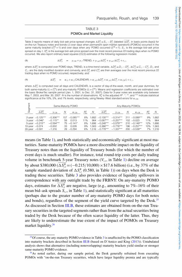
Pasquariello, Roush, and Vega 139
TABLE 3POMOs and Market Liquidity
Table 3 reports means of daily bid–ask price spread changes 1SBi ,t ≡Si ,t −SBi ,t (labeled 1S
Bi ,t , in basis points (bps)) for
on-the-run Treasury notes and bonds (i ) over days when permanent open market operations (POMOs) occurred in thesame maturity bracket (ICBi ,t =1) and over days when any POMO occurred (ICBt =1). Si ,t is the average bid–ask pricespread on day t ; SBi ,t is the average bid–ask price spread over the most recent previous 22 trading days when no POMOoccurred. We also report ordinary least squares (OLS) estimates of the following regression models:
(8) 1SBi ,t = γi ,CB + γi ,T TRENDt + γi ,1D1DBi ,t + γi ,1C1C
Bi ,t + εi ,t ,
where 1SBi ,t is computed over POMO days, TRENDt is a time-trend variable, 1DBi ,t ≡Di ,t −D
Bi ,t , 1C
Bi ,t ≡Ci ,t −C
Bi ,t , Di ,t and
Ci ,t are the daily modified duration and convexity, and DBi ,t and C
Bi ,t are their averages over the most recent previous 22
trading days when no POMO occurred, respectively; and
(9) 1SBi ,t = αi ,0 +αi ,CCALENDARt +αi ,1D1DBi ,t +αi ,1C1C
Bi ,t +αi ,CBIt + εi ,t ,
where 1SBi ,t is computed over all days and CALENDARt is a vector of day-of-the-week, month, and year dummies, forboth same-maturity (It = ICBi ,t ) and any-maturity POMOs (It = ICBt ). Means and regression coefficients are estimated overthe basic BrokerTec sample period (Jan. 1, 2001, to Dec. 31, 2007). Data for 3-year notes are available only betweenMay 7, 2003, and Mar. 30, 2007. N is the number of observations. R 2
a is the adjusted R 2. *, **, and *** indicate statisticalsignificance at the 10%, 5%, and 1% levels, respectively, using Newey–West standard errors for αi ,CB.
Same-Maturity POMO Any-Maturity POMOs
Segm
ent
1SBi ,t γi ,CB N αi ,CB R 2a N 1SBi ,t γi ,CB N αi ,CB R 2
a N
2-year −0.125*** −0.306*** 157 −0.085*** 8% 1,682 −0.130*** −0.314*** 211 −0.089*** 9% 1,6823-year −0.046* −0.115** 58 0.013 11% 964 −0.087*** −0.257*** 102 −0.023 11% 9645-year −0.215** −0.594*** 75 −0.141* 8% 1,686 −0.248*** −0.579*** 210 −0.149*** 12% 1,686
10-year −0.074 −0.002 33 0.028 9% 1,563 −0.366*** −0.776*** 196 −0.257*** 10% 1,56330-year −0.591 −1.316 28 −0.294 6% 1,516 −0.778*** −1.337*** 200 −0.539** 7% 1,516
means (in Table 1), and both statistically and economically significant at most ma-turities. Same-maturity POMOs have a more discernible impact on the liquidity ofTreasury notes than on the liquidity of Treasury bonds (for which the number ofevent days is much smaller). For instance, total round-trip costs per daily tradingvolume in benchmark 5-year Treasury notes (Vi ,t , in Table 1) decline on averageby about $380,000 (1SB
i ,t=(−0.215/10,000)×$17.6 billion) (i.e., by 37% of thesample standard deviation of 1SB
i ,t (0.580, in Table 1)) on days when the Desk istrading these securities. Table 3 also provides evidence of liquidity spillovers incorrespondence with any outright trade by the FRBNY: On any-maturity POMOdays, estimates for 1SB
i ,t are negative, large (e.g., amounting to 7%–16% of theirmean bid–ask spreads Si ,t , in Table 1), and statistically significant at all maturities(perhaps due to the greater number of any-maturity POMO days for both notesand bonds), regardless of the segment of the yield curve targeted by the Desk.25
As discussed in Section III.B, these estimates are obtained from on-the-run Trea-sury securities in the targeted segments rather than from the actual securities beingtraded by the Desk because of the often scarce liquidity of the latter. Thus, theyare likely to underestimate the true extent of the impact of POMOs on Treasurymarket liquidity.26
25Of course, the any-maturity POMO evidence in Table 3 is unaffected by the POMO classificationinto maturity brackets described in Section III.B (based on D’Amico and King (2013)). Untabulatedanalysis shows that alternative (including nonoverlapping) maturity brackets yield similar or strongersame-maturity POMO evidence.
26As noted earlier, during our sample period, the Desk generally refrained from executingPOMOs with “on-the-run Treasury securities, which have larger liquidity premia and are typically
https://doi.org/10.1017/S0022109018001552D
ownloaded from
https://ww
w.cam
bridge.org/core . Univ of M
ichigan Law Library , on 08 Jan 2020 at 16:38:34 , subject to the Cam
bridge Core terms of use, available at https://w
ww
.cambridge.org/core/term
s .

140 Journal of Financial and Quantitative Analysis
Improvements in Treasury market liquidity in proximity to POMOs may bedue to changes in bond characteristics and calendar effects unrelated to FRBNYinterventions. For instance, changes in Treasury securities’ sensitivity to yield dy-namics (as proxied by modified duration, Di ,t , and convexity, Ci ,t ) may affect theirperceived riskiness to dealers and investors (e.g., Strebulaev (2002), Goldreichet al. (2005), and Pasquariello and Vega (2009)). Bid–ask spreads and tradingactivity also display weekly seasonality and time trends (e.g., Fleming (1997),(2003), Pasquariello and Vega (2007)). In particular, as noted previously, bid–ask spreads on the BrokerTec platform have considerably tightened (and tradingvolume has likewise increased) over our sample period, especially from 2005 on-ward. These effects may either enhance or distort the impact of POMOs on theprocess of price formation in the Treasury bond market.
We assess the robustness of our univariate inference to these considerationsby specifying a multiple regression event-study model of bid–ask price spreadchanges, that is, for only same-maturity (I CB
i ,t =1) or any-maturity POMO days(I CB
t =1), as follows:
(8) 1SBi ,t = γi ,C B + γi ,T TRENDt + γi ,1D1DB
i ,t + γi ,1C1C Bi ,t + εi ,t ,
where TRENDt is a time-trend variable,1DBi ,t≡Di ,t−DB
i ,t ,1C Bi ,t≡Ci ,t−C B
i ,t , andDB
i ,t and C Bi ,t are average modified duration and convexity over the most recent
previous 22 trading days when no POMO occurred, respectively. We consideradditional explicit controls in Section 2.4 of the Supplementary Material (see alsoSection IV.B). Estimates of the intercept γi ,CB in equation (8) measure averagechanges in Treasury bid–ask spreads on POMO days (i.e., relative to the prior 22non-POMO days) net of calendar effects and contemporaneous changes in bondcharacteristics. We also specify a similar model using all trading days:
1SBi ,t = αi ,0+αi ,C CALENDARt +αi ,1D1DB
i ,t(9)+αi ,1C1C B
i ,t +αi ,CB It + εi ,t ,
where either It= I CBi ,t or It= I CB
t and CALENDARt is a vector of day-of-the-week,month, and year dummies.27 Estimates of the event dummy coefficient αi ,CB inequation (9) capture any additional effect of POMOs on 1SB
i ,t relative to its aver-age over all other trading days in the sample period (i.e., the constant αi ,0).
We estimate equations (8) and (9) for each on-the-run maturity in ourdatabase separately using ordinary least squares (OLS). We evaluate the statisticalsignificance of the coefficients’ estimates, reported in Table 3, with Newey–Weststandard errors to correct for heteroskedasticity and serial correlation. The resultsin Table 3 provide further support for our model’s main prediction. Consistentwith the prior univariate evidence, bid–ask spreads tend to decline (i.e., γi ,CB<0
most susceptible to liquidity squeezes, so as to avoid adverse market impact” (FRBNY (2005), p. 20).Specifically, the Desk never executed POMOs with on-the-run securities over the pre-crisis period(2001–2007) and purchased only six of them (one per separate POMO day) during the financial crisisperiod (2008–2009) (versus an average of 73 Treasury securities per POMO day over 75 POMO days;Panel D of Table 2) (see also the discussion in Sections 2.2 and 2.4 of the Supplementary Material).
27The time series Si ,t are made of several on-the-run securities stacked on one another over thesample period (as in Brandt and Kavajecz (2004), Green (2004), and Pasquariello and Vega (2007),(2009)). Unreported analysis shows our inference to be insensitive to the inclusion of security fixedeffects in equations (8) and (9).
https://doi.org/10.1017/S0022109018001552D
ownloaded from
https://ww
w.cam
bridge.org/core . Univ of M
ichigan Law Library , on 08 Jan 2020 at 16:38:34 , subject to the Cam
bridge Core terms of use, available at https://w
ww
.cambridge.org/core/term
s .

Pasquariello, Roush, and Vega 141
and αi ,CB<0) both when same-maturity and any-maturity POMOs occur, and thisdecline is especially significant for the latter (i.e., in correspondence with liquid-ity spillovers and a greater number of any-maturity POMO days). Controlling forcalendar effects and bond characteristics strengthens our inference: For instance,all estimated intercepts γi ,CB in equation (8) are larger (in absolute magnitude)than the corresponding means 1SB
i ,t . As in prior event-study research, POMOs’liquidity externalities are instead smaller when estimated over all trading days(i.e.,
∣∣αi ,CB
∣∣< ∣∣γi ,CB
∣∣). Regardless of the methodology used, the estimated declinein bid–ask spread accompanying POMO days remains both statistically and eco-nomically significant (e.g., amounting on average to 53% (14%) of the corre-sponding sample mean (in Table 1), and to more than 50% (25%) of the standarddeviation of the corresponding spread change (also in Table 1), when measuredby γi ,C B (αi ,CB)).
Last, we note that our empirical strategy follows Harvey and Huang (2002)in that we use an indicator variable for POMO days rather than estimate the effectof the magnitude of POMOs on Treasury market liquidity. As Harvey and Huangemphasize, such an estimation is problematic since the econometrician does notknow how much of each POMO trade is unexpected by market participants.28
In addition, our model predicts that the mere presence of government interventionimproves market liquidity (Conclusion 1). However, both the actual central banktrade (xCB) and market depth (1/λCB) are endogenously determined in equilib-rium, as for any strategic order flow in Kyle (1985). Accordingly, most empiricalliterature advocates the use of order imbalance (number of transactions per pe-riod, in the spirit of equations (8) and (9)) instead of trading volume when assess-ing the impact of order flow on price formation in financial markets (see, e.g.,Hasbrouck (1991), (2007), Jones, Kaul, and Lipson (1994), Evans and Lyons(2002), Chordia and Subrahmanyam (2004), Green (2004), Pasquariello andVega (2007), Chordia, Hu, Subrahmanyam, and Tong (2019), and Pasquariello(2018)).29
B. POMOs and Market Liquidity: RobustnessThe evidence in Table 3 suggests that Treasury market liquidity improves
on POMO days, consistent with the main prediction of our model. In Section 2of the Supplementary Material, we assess the robustness of this evidence and itsconformity to alternative interpretations.
28For instance, the FRBNY has only recently begun to preannounce monthly and daily ex-pected POMO amounts, while executing extraordinary monetary policy measures in the aftermathof the 2008–2009 financial crisis (i.e., since Aug. 2010, at https://www.newyorkfed.org/markets/totoperation schedule.html; see also Section 2.2 of the Supplementary Material and Section IV.B). Es-timating those amounts would introduce generated-regressor biased standard errors in our empiricalanalysis. We nonetheless develop a proxy for uncertainty surrounding POMO policy in Section IV.C.3.The ensuing evidence suggests that our baseline empirical results in Table 3 are only weakened by as-suming uniform POMO policy uncertainty on every POMO day in our sample.
29For example, when studying the microstructure of the U.S. stock market, (Jones et al. (1994),p. 631) find that “it is the occurrence of transactions per se, and not their size, that generates[price] volatility; trade size has no information beyond that contained in the frequency [i.e., number]of transactions.” (Hasbrouck (2007), p. 90) attributes such findings to the fact that, as in our modelof Section II, “agents trade large amounts when price impact is low, and small amounts when priceimpact is high.” See also the discussion in Pasquariello (2018).
https://doi.org/10.1017/S0022109018001552D
ownloaded from
https://ww
w.cam
bridge.org/core . Univ of M
ichigan Law Library , on 08 Jan 2020 at 16:38:34 , subject to the Cam
bridge Core terms of use, available at https://w
ww
.cambridge.org/core/term
s .

142 Journal of Financial and Quantitative Analysis
In particular, we find our inference to be qualitatively similar yet strongerwithin the earlier portion of our sample (2001–2004), when bid–ask spreads aremuch wider and more volatile, than in the calmer latter period (2005–2007), aswell as robust to extending our analysis to all available GovPX data within oursample period (i.e., over 2001–2004) to account for the aforementioned gradualmigration of most trading in on-the-run Treasury securities from voice-brokered(GovPX) to electronic intermediation (BrokerTec and eSpeed) (see Section 2.1and Table IA1 of the Supplementary Material). We also find that the estimatedliquidity externalities of the more numerous and larger POMOs executed duringthe recent financial crisis (2008–2009; Panel D of Table 2 and Figure 3) are con-sistent with our model’s main prediction in Conclusion 1, despite the ensuingeconomic and financial turmoil (see, e.g., Figure 4) and likely effects on both liq-uidity provision (otherwise worsening; Figure 2 and Panel D of Table 1) and theFederal Reserve’s policy goals in the Treasury market (see Section 2.2 and TableIA2 of the Supplementary Material).
We then ascertain that our inference is robust to such alternative specifica-tions as the estimation of1SB
i ,t , γi ,CB, and αi ,CB over different pre-intervention peri-ods, during the intraday 90-minute Fed Time interval when the FRBNY typicallyannounces and executes its POMOs (10:00AM to 11:30AM; see Section III.B) aswell as for percentage bid–ask spreads Si≡(Ai− Bi)/
[12 (Ai+ Bi)
](see Section
2.3 and Table IA3 of the Supplementary Material). Last, we consider several alter-native interpretations of the evidence in Table 3 related to Treasury market condi-tions during POMO activity (like dealers’ inventory levels, pre-auction illiquidity,bank reserves, or relative security supply) and show that our inference is robustto explicitly controlling for such additional factors related to those conditions asrepo specialness, Treasury auction outcomes, pre–Fed Time and end-of-year on-the-run illiquidity, the Desk’s repo-trading activity, reserve maintenance periods,dates of and distance from FOMC meetings, and the release of important U.S.macroeconomic announcements (listed in Section IV.C.1), hence mitigating po-tential omitted variable biases in that inference (notwithstanding the discussion inSection I) (see Section 2.4 and Table IA4 of the Supplementary Material).
C. POMOs and the Information Environment of the MarketThe evidence in Table 3 provides support for our model’s main prediction
(in Conclusion 1): POMOs executed by the FRBNY’s Desk in the secondary mar-ket for Treasury securities meaningfully improve Treasury market liquidity. Ourmodel attributes this effect to the impact of government intervention on the Trea-sury market’s information environment. In this section, we assess more directlythis basic, novel premise of our theory by testing its unique, additional predictionsfor Treasury market liquidity (also in Conclusion 1).
1. Information Heterogeneity
The first prediction from Conclusion 1 states that, ceteris paribus, greater in-formation heterogeneity among speculators (i.e., lower ρ) magnifies the positiveliquidity externalities of government intervention (i.e., a more negative 1λ, asin Graph C of Figure 1). Intuitively, more heterogeneously informed speculatorstrade more cautiously to protect their perceived private information monopoly.
https://doi.org/10.1017/S0022109018001552D
ownloaded from
https://ww
w.cam
bridge.org/core . Univ of M
ichigan Law Library , on 08 Jan 2020 at 16:38:34 , subject to the Cam
bridge Core terms of use, available at https://w
ww
.cambridge.org/core/term
s .

Pasquariello, Roush, and Vega 143
FIGURE 4Marketwide Information Variables
Figure 4 plots SSDFq (Graph A), the scaled simple average of standardized standard deviation of professional fore-casts of six U.S. macroeconomic variables (unemployment, nonfarm payroll, nominal gross domestic product (GDP),consumer price index (CPI), industrial production, and housing starts) from the Survey of Professional Forecasters (SPF,see Section IV.C.1); SSDNFm (Graph B), the scaled standardized standard deviation of professional forecasts of nonfarmpayroll from Bloomberg (Section IV.C.1); EURVOLm (Graph C), the monthly average of daily Eurodollar implied volatility(in percentage) from Bloomberg (Section IV.C.2); TOVOLm (Graph D), the monthly average of daily implied volatility on1-month Treasury options from Merrill Lynch (Section IV.C.2); FEDVOLm (Graph E), the monthly average of daily volatilityof the federal funds rate (in percentage) from the Federal Reserve Bank of New York (FRBNY) (Section IV.C.3), betweenJan. 2001 and Dec. 2009.
4.0
4.5
5.0
5.5
SS
DF q
EU
RV
OL m
TOV
OL m
FED
VO
L m
SS
DN
F m
6.0
6.5
7.0Graph A. SSDFq
Graph C. EURVOLm
Graph E. FEDVOLm
Graph D. TOVOLm
Graph B. SSDNFm
Date
Jan.-
01
June
-02
Dec.-0
3
June
-05
Dec.-0
6
June
-08
Dec.-0
9
Date
Jan.-
01
June
-02
Dec.-0
3
June
-05
Dec.-0
6
June
-08
Dec.-0
9
Date
Jan.-
01
June
-02
Dec.-0
3
June
-05
Dec.-0
6
June
-08
Dec.-0
9
Date
Jan.-
01
June
-02
Dec.-0
3
June
-05
Dec.-0
6
June
-08
Dec.-0
93
4
5
6
7
8
0.0
0.1
0.2
0.3
0.4
0.5
0.6
0.7
0.0
0.1
0.2
0.3
0.4
0.5
0.6
0.7
507090
110130150170190210230
Date
Jan.-
01
June
-02
Dec.-0
3
June
-05
Dec.-0
6
June
-08
Dec.-0
9
The ensuing greater adverse selection risk for the MMs worsens market liquid-ity (i.e., increases the equilibrium price impact of aggregate order flow). In thosecircumstances, central bank trades attempting to achieve a nonpublic, uninforma-tive policy target more significantly mitigate the more severe threat of adverseselection in market-making.
https://doi.org/10.1017/S0022109018001552D
ownloaded from
https://ww
w.cam
bridge.org/core . Univ of M
ichigan Law Library , on 08 Jan 2020 at 16:38:34 , subject to the Cam
bridge Core terms of use, available at https://w
ww
.cambridge.org/core/term
s .

144 Journal of Financial and Quantitative Analysis
Testing for this prediction requires measurement of the heterogeneity ofprivate information about fundamentals among sophisticated Treasury marketparticipants. Marketwide information heterogeneity is commonly proxied by thestandard deviation across professional forecasts of economic and financial vari-ables (e.g., Diether, Malloy, and Scherbina (2002), Green (2004), and Yu (2011)).In this article we consider two proxies for ρ based on the notion that U.S. macroe-conomic variables may contain payoff-relevant information for U.S. Treasury se-curities; accordingly, numerous studies find that government bond returns andmarket quality are sensitive to the release of these variables to the public (e.g., seePasquariello and Vega (2007), Brenner, Pasquariello, and Subrahmanyam (2009),and references therein). These proxies employ the only continuously availablesurveys of U.S. macroeconomic forecasts over our sample period, namely thosecollected by the Federal Reserve Bank of Philadelphia (the Survey of ProfessionalForecasters (SPF)) and by Bloomberg.
The SPF, initiated in 1968 by the American Statistical Association and theNational Bureau of Economic Research, is commonly used in empirical researchon the formation of macroeconomic expectations. Croushore (1993) provides adetailed description of the SPF database. SPF data are available exclusively at thequarterly frequency. For each quarter q , the SPF database contains tens of indi-vidual forecasts by private sector economists (working at financial firms, banks,economic consulting firms, university research centers, and Fortune 500 compa-nies) for various macroeconomic variables and at various future horizons. Wefocus on next-quarter forecasts for the most important of them: nonfarm payroll,unemployment, nominal gross domestic product (GDP), consumer price index(CPI), industrial production, and housing starts (e.g., Andersen and Bollerslev(1998), Andersen et al. (2003), (2007), Pasquariello and Vega (2007), Brenneret al. (2009), and Gilbert, Scotti, Strasser, and Vega (2017); see also Section 2.4 ofthe Supplementary Material and Section IV.B). Bloomberg surveys professionalforecasts of U.S. macroeconomic announcements at the frequency of their releaseto the public. These data are available to us only for nonfarm payroll, which isreleased monthly and is labeled by (Andersen and Bollerslev (1998), p. 240) asthe “king” of macroeconomic announcements because of its significant impact onfinancial markets.
We define the dispersion of beliefs among speculators for each macroeco-nomic variable p in the SPF data set in quarter q as the standard deviation of allof that variable’s next-quarter forecasts available in that quarter, SDFp,q . We sim-ilarly compute the monthly standard deviation of all of the nonfarm payroll fore-casts available in Bloomberg in month m, SDNFm . Since units of measurementdiffer across macroeconomic variables, we then divide the difference betweeneach SDFp,q (or SDNFm) and its sample mean by its sample standard deviation(e.g., Pasquariello and Vega (2007)) and then add 5 (to ensure that each infor-mation variable is always positive). This yields time series of scaled, standardizeddispersion of analyst forecasts, SSDFp,q and SSDNFm . Last, we compute our prox-ies for the aggregate degree of information heterogeneity about U.S. macroeco-nomic fundamentals as either SSDFq (the simple average of all available SSDFp,q ;see Graph A of Figure 4) or SSDNFm (see Graph B), such that the greater eitherproxy is, the lower ρ may be in the U.S. Treasury market.
https://doi.org/10.1017/S0022109018001552D
ownloaded from
https://ww
w.cam
bridge.org/core . Univ of M
ichigan Law Library , on 08 Jan 2020 at 16:38:34 , subject to the Cam
bridge Core terms of use, available at https://w
ww
.cambridge.org/core/term
s .

Pasquariello, Roush, and Vega 145
As in Section IV.A, we assess the impact of marketwide informationheterogeneity on POMOs’ positive liquidity externalities in several ways. Weestimate univariate regressions of average bid–ask spread changes 1SB
i ,t over(same-maturity or any-maturity) POMO days alone (I CB
i ,t =1 or I CBt =1) on the
contemporaneous realizations of either X t=SSDFq or X t=SSDNFPm :
(10) 1SBi ,t = βi ,CB+β
xi ,CB X t + εi ,t .
We also amend the multiple regression models of equations (8 ) and (9) to includeeither the information variable X t (SSDFq or SSDNFPm) using only POMO days:
1SBi ,t = γi ,C B + γi ,T CALENDARt + γi ,1D1DB
i ,t(11)+γi ,1C1C B
i ,t + γx
i ,C B X t + εi ,t ,
or both X t and its cross-products with same-maturity and any-maturity POMOdummies (It= I CB
i ,t and It= I CBt ) using all trading days:
1SBi ,t = αi ,0+αi ,C CALENDARt +αi ,1D1DB
i ,t +αi ,1C1C Bi ,t +αi ,x X t(12)
+αi ,CB It +αxi ,CB It X t + εi ,t .
Estimates of the slope coefficient β xi ,CB in equation (10) capture any state depen-
dency (from X t ) in bid–ask spread changes on POMO days alone. Estimates of theinteraction coefficient γ x
i ,CB in equation (11) capture that state dependency whilecontrolling for calendar effects and changes in bond characteristics. Estimates ofthe interaction coefficient αx
i ,CB in equation (12) capture that state dependency withrespect to changes over the whole sample period.30
The linear specifications of equations (10)–(12) are standard in the litera-ture (e.g., see Pasquariello and Vega (2015), Pasquariello (2018)) and allow usto estimate the statistical significance of the continuous effect of any state vari-able X t on POMOs’ liquidity externalities. However, the scale of X t affects thescale of the resulting OLS estimates for β x
i ,CB, γ xi ,CB, and αx
i ,CB. Thus, exclusivelyto ease their interpretation and assess their economic significance, we multiplyeach of those coefficients by a hypothetical discrete increase in the informa-tion variable X t from the bottom (i.e., “low”) 30th percentile (X 30th
t ) to the top(i.e., “high”) 70th percentile (X 70th
t ) of its empirical distribution. We report thesescaled estimates 11SB,x
i ,t ≡βxi ,CB
(X 70th
t − X 30tht
), 1γ x
i ,CB≡γx
i ,CB
(X 70th
t − X 30tht
), and
1αxi ,CB≡α
xi ,CB
(X 70th
t − X 30tht
)for either X t=SSDFq or X t=SSDNFPm in Panels A
and B of Table 4, respectively. By construction,11SB,xi ,t ,1γ x
i ,CB, and1αxi ,CB are in
the same unit as the dependent variable 1SBi ,t (i.e., bps); their sign and statistical
significance are unaffected by alternative scaling factors (e.g., different high–lowranges for X t or the sample standard deviation of X t ).
30According to our basic model (see Proposition 1, in Section II.A) and extant empirical evidence(e.g., Pasquariello and Vega (2007)), the Treasury market’s information environment may affect itsequilibrium liquidity (λ of equation (3)) even in the absence of central bank interventions (i.e., evenon non-POMO days). Thus, our low-frequency information measures X t are likely to impact both Si ,t
and SBi ,t , such that these effects may cancel out in1SB
i ,t≡ Si ,t− SBi ,t . Consistently, untabulated estimates
of αi ,x in equation (12) reveal 1SBi ,t to be largely insensitive to X t on non-POMO days.
https://doi.org/10.1017/S0022109018001552D
ownloaded from
https://ww
w.cam
bridge.org/core . Univ of M
ichigan Law Library , on 08 Jan 2020 at 16:38:34 , subject to the Cam
bridge Core terms of use, available at https://w
ww
.cambridge.org/core/term
s .

146 Journal of Financial and Quantitative Analysis
TABLE 4POMOs and Information Heterogeneity
Table 4 reports ordinary least squares (OLS) slope coefficients βxi ,CB of the following regression of average daily bid–ask spread and price changes 1SBi ,t (in basis points (bps), defined in Section IV.A) for on-the-run Treasury notes andbonds (i ) over same -maturity or any -maturity permanent open market operation (POMO) days (ICBi ,t =1 or ICBt =1 ) on thecontemporaneous realizations of either Xt =SSDFq (the simple scaled average of the standardized dispersion of analystforecasts of six macroeconomic variables from the Survey of Professional Forecasters (SPF), see Section IV.C.1; in PanelA) or Xt =SSDNFm (the scaled standardized dispersion of analyst forecasts of nonfarm payroll from Bloomberg, seeSection IV.C.1; in Panel B) multiplied by the difference between X 70th
t (the top 70th percentile of its empirical distribution)and X 30th
t (the bottom 30th percentile of its empirical distribution):
(10) 1SBi ,t = βi ,CB +βxi ,CBXt + εi ,t .
We label these differences as 11SB ,xi ,t ≡βxi ,CB
(X 70tht −X 30th
t
). We also estimate, again by OLS, both the effect of either
Xt =SSDFq or Xt =SSDNFm on 1SBi ,t in event time (slope γ xi ,CB):
(11) 1SBi ,t = γi ,CB + γi ,T TRENDt + γi ,1D1DBi ,t + γi ,1C1C
Bi ,t + γ
xi ,CBXt + εi ,t ,
as well as the interaction of either It = ICBi ,t or It = ICBt with either Xt =SSDFq or Xt =SSDNFm over the full sample (interactionαxi ,CB):
(12) 1SBi ,t = αi ,0 +αi ,CCALENDARt +αi ,1D1DBi ,t +αi ,1C1C
Bi ,t +αi ,xXt +αi ,CBIt +α
xi ,CB ItXt + εi ,t .
We report these slope and interaction coefficients as1γ xi ,CB≡γxi ,CB
(X 70tht −X 30th
t
)and1αxi ,CB≡α
xi ,CB
(X 70tht −X 30th
t
), again in
bps. Means and regression coefficients are estimated over the basic BrokerTec sample period (Jan. 1, 2001, to Dec. 31,2007). Data for 3-year notes are available only between May 7, 2003, and Mar. 30, 2007. N is the number of observations.R 2a is the adjusted R 2. *, **, and *** indicate statistical significance at the 10%, 5%, or 1% levels, respectively, using
Newey–West standard errors for αxi ,CB.
Same-Maturity POMOs Any-Maturity POMOs
Segm
ent
11SB ,xi ,t 1γ xi ,CB N 1αxi ,CB R 2a N 11SB ,xi ,t 1γ xi ,CB N 1αxi ,CB R 2
a N
Panel A. Xt =SSDFq
2-year −0.099*** −0.061*** 157 −0.086*** 9% 1,682 −0.107*** −0.067*** 211 −0.092*** 11% 1,6823-year 0.011 0.003 58 0.014 10% 964 −0.023 −0.047** 102 −0.017 11% 9645-year −0.220*** −0.150 75 −0.172 9% 1,686 −0.206*** −0.137*** 210 −0.167*** 13% 1,686
10-year −0.274* −0.461* 33 −0.297* 9% 1,563 −0.361*** −0.248*** 196 −0.295*** 11% 1,56330-year −1.537** −1.897* 28 −1.664** 7% 1,516 −0.247 −0.051 200 −0.373 7% 1,516
Panel B. Xt =SSDNFm
2-year −0.064*** −0.065*** 157 −0.056** 9% 1,682 −0.068*** −0.015** 211 −0.058** 10% 1,6823-year 0.002 0.008 58 0.006 11% 964 −0.008 −0.028* 102 0.018 11% 9645-year 0.080 0.096 75 0.059 9% 1,686 −0.074* −0.051 210 −0.062 12% 1,686
10-year −0.337* −0.329 33 −0.282 9% 1,563 −0.117** −0.011 196 −0.118** 10% 1,56330-year −0.425 −0.541 28 −0.223 6% 1,516 −0.098 −0.069 200 0.075 7% 1,516
Consistent with Conclusion 1, POMOs’ positive liquidity externalities areincreasing in our proxies for marketwide information heterogeneity (i.e., decreas-ing in ρ) (11SB,x
i ,t , 1γ xi ,CB, and 1αx
i ,CB are negative and statistically significant)in correspondence with both same-maturity (I CB
i ,t =1) and any-maturity POMOs(I CB
t =1) for both on-the-run Treasury notes and bonds. For instance, Panel A ofTable 4 shows that, on average, bid–ask spreads for 2-year, 5-year, and 10-yearTreasury notes on any-maturity POMO days when our broad-based proxy formarketwide dispersion of beliefs X t=SSDFq is high decline by roughly 110%(of the baseline effect in Table 3) more (or about 0.185 bps more) than whenSSDFq is low (i.e., mean significant 1αx
i ,CB/αi ,CB=1.10). Panel A of Table 4 fur-ther indicates that, in correspondence with government intervention at the long-end of the yield curve, bid–ask spreads for 30-year Treasury bonds when SSDFq
is high are nearly 2 bps lower than when SSDFq is low (i.e., 11SB,xi ,t =−1.537,
1γ xi ,CB=−1.897, and1αx
i ,CB=−1.664). Those estimates are qualitatively similar,
https://doi.org/10.1017/S0022109018001552D
ownloaded from
https://ww
w.cam
bridge.org/core . Univ of M
ichigan Law Library , on 08 Jan 2020 at 16:38:34 , subject to the Cam
bridge Core terms of use, available at https://w
ww
.cambridge.org/core/term
s .

Pasquariello, Roush, and Vega 147
albeit smaller and less often statistically significant, when obtained from the (nois-ier) monthly series of dispersion of nonfarm payroll forecasts alone (i.e., whenX t=SSDNFm ; see Graph B of Figure 4) in Panel B. This evidence suggests thatgovernment interventions have a greater impact on the process of price formationin the secondary market for Treasury securities when information heterogeneityamong speculators is high, as postulated by our model.
2. Fundamental Uncertainty
The second prediction from Conclusion 1 states that, ceteris paribus, greateruncertainty about the traded asset’s payoff (i.e., higher σ 2
v) amplifies the impact
of government intervention on market liquidity (i.e., leads to higher |1λ| (GraphD of Figure 1)). Greater fundamental uncertainty worsens equilibrium market liq-uidity because it makes speculators’ private information more valuable and theaccompanying adverse selection risk for the MMs more severe. As discussed pre-viously, this enhances the positive liquidity externalities of central bank trades.
To evaluate this implication of our model, we use two proxies for σ 2v. The
first is EURVOLm (plotted in Graph C of Figure 4), the monthly average (tosmooth daily variability) of daily Eurodollar implied volatility from Bloomberg.The second is TOVOLm (in Graph D of Figure 4), the monthly average of dailyrealizations of the yield-curve-weighted MOVE index of the normalized impliedvolatility on 1-month Treasury options from Merrill Lynch. Both EURVOLm
and TOVOLm are commonly used as measures of market participants’ perceiveduncertainty surrounding U.S. macroeconomic fundamentals (e.g., Bernanke andKuttner (2005), Pasquariello and Vega (2009)). We then run the same uni-variate and multiple regressions for spread change differentials described inSection IV.C.1, which yield scaled estimates 11SB,x
i ,t for the former, 1γ xi ,CB and
1αxi ,CB for the latter, after imposing that either X t=EURVOLm or X t=TOVOLm .
We report these estimates in Panels A and B of Table 5, respectively.Consistent with Conclusion 1, 11SB,x
i ,t , 1γ xi ,CB, and 1αx
i ,CB are always neg-ative in Table 5 and nearly always statistically significant when proxying forfundamental uncertainty with X t=TOVOLm . For example, Panel B of Table 5shows that during any-maturity POMO days when TOVOLm is historically high,the bid–ask spreads for 10-year Treasury notes decline by roughly 0.3 bps morethan when TOVOLm is low (i.e., a statistically significant 11SB,x
i ,t =−0.309,1γ x
i ,CB=−0.271, and1αxi ,CB=−0.295). This effect is economically significant as
well because it amounts to roughly 32% of the sample standard deviation of1SBi ,t
in Table 1. Those estimates are rarely statistically significant for X t=EURVOLm ,in Panel A of Table 5. However, in those circumstances bid–ask spreads tightenmuch more pronouncedly on POMO days characterized by higher Eurodollarvolatility (e.g., by no less than 100% of the baseline decline in spread reportedin Table 3). This evidence suggests that government interventions are accompa-nied by a greater improvement in Treasury market liquidity when fundamentaluncertainty is greater, as implied by our model.
3. POMO Policy Uncertainty
The last prediction from Conclusion 1 states that, ceteris paribus, greater un-certainty about the central bank’s uninformative policy target pT among market
https://doi.org/10.1017/S0022109018001552D
ownloaded from
https://ww
w.cam
bridge.org/core . Univ of M
ichigan Law Library , on 08 Jan 2020 at 16:38:34 , subject to the Cam
bridge Core terms of use, available at https://w
ww
.cambridge.org/core/term
s .

148 Journal of Financial and Quantitative Analysis
TABLE 5POMOs and Fundamental Uncertainty
Table 5 reports ordinary least squares (OLS) estimates of the slope coefficient βxi ,CB from equation (10) and the interactioncoefficients γ xi ,CB and αxi ,CB from equations (11) and (12) for on-the-run Treasury notes and bonds and same-maturity orany -maturity permanent open market operations (POMOs, as in Table 4) over the basic BrokerTec sample period (Jan.1, 2001, to Dec. 31, 2007) when either Xt =EURVOLm (the monthly average of daily Eurodollar implied volatility fromBloomberg, see Section IV.C.2; in Panel A) or Xt =TOVOLm (the monthly average of daily implied volatility on Treasury op-tions fromMerrill Lynch, see Section IV.C.2; in Panel B), multiplied by the difference between X 70th
t (the top 70th percentileof its empirical distribution) and X 30th
t (the bottom 30th percentile of its empirical distribution). We label these differences
(in basis points (bps)) as11SB ,xi ,t ≡βxi ,CB
(X 70tht −X 30th
t
),1γ xi ,CB ≡γ
xi ,CB
(X 70tht −X 30th
t
), and1αxi ,CB≡α
xi ,CB
(X 70tht −X 30th
t
). N is
the number of observations. R 2a is the adjusted R 2. *, **, and *** indicate statistical significance at the 10%, 5%, or 1%
levels, respectively, using Newey–West standard errors for αxi ,CB.
Same-Maturity POMOs Any-Maturity POMOs
Segm
ent
11SB ,xi ,t 1γ xi ,CB N 1αxi ,CB R 2a N 11SB ,xi ,t 1γ xi ,CB N 1αxi ,CB R 2
a N
Panel A. Xt =EURVOLm
2-year −0.015 −0.091*** 157 −0.027 9% 1,682 −0.026 −0.076*** 211 −0.034 10% 1,6823-year −0.051* −0.008 58 −0.025 10% 964 −0.130*** 0.024 102 −0.086** 11% 9645-year −0.039 −0.154 75 −0.060 9% 1,686 −0.023 −0.182*** 210 −0.049 13% 1,686
10-year −0.398 −0.513 33 −0.323*** 9% 1,563 −0.123 0.192 196 −0.154** 11% 1,56330-year −0.898 −1.171 28 −0.479 7% 1,516 −0.452 −0.246 200 −0.340 8% 1,516
Panel B. Xt =TOVOLm
2-year −0.102*** −0.107*** 157 −0.093*** 9% 1,682 −0.117*** −0.123*** 211 −0.102*** 10% 1,6823-year −0.076** −0.069* 58 −0.049 11% 964 −0.159*** −0.150*** 102 −0.126*** 12% 9645-year −0.198* −0.206* 75 −0.176** 9% 1,686 −0.185*** −0.176** 210 −0.147*** 12% 1,686
10-year −0.355 −0.301 33 −0.372*** 9% 1,563 −0.309*** −0.271*** 196 −0.295*** 11% 1,56330-year −1.500 −1.959 28 −1.407** 6% 1,516 −0.584 −0.652* 200 −0.578** 7% 1,516
participants (i.e., higher σ 2T ) enhances the improvement in equilibrium market liq-
uidity accompanying its trades (1λ, as in Graph B of Figure 1). Greater policyuncertainty complicates the MMs’ attempt at accounting for the extent of unin-formative government intervention in the aggregate order flow before setting theequilibrium price p1. However, it also lowers their perceived adverse selectionrisk from trading with informed speculators.
As discussed in Sections II.B and III.B, the FRBNY’s Desk targets the ag-gregate level of nonborrowed reserves available in the banking system via unin-formative POMOs to ensure that conditions in the federal funds rate market are“consistent” with the publicly known target rate set by the FOMC.31 Thus, un-certainty among market participants about the FRBNY’s nonpublic and uninfor-mative reserve target for POMOs may manifest itself in the federal funds market.Accordingly, we measure marketwide policy uncertainty surrounding the Desk’sPOMOs with FEDVOLm (plotted in Graph E of Figure 4), the monthly average(to smooth daily variability) of daily standard deviation of the federal funds rate,from the FRBNY (these data are available at https://apps.newyorkfed.org/markets/autorates/fed%20funds). Importantly, in unreported analysis we find FEDVOLm
to be virtually unrelated to our proxies for marketwide dispersion of beliefs(ρ) and uncertainty (σ 2
v) about U.S. macroeconomic fundamentals described in
Sections IV.C.1 and IV.C.2. We then assess the sensitivity of spread changes in
31For example, the Web site of the FRBNY (https://www.newyorkfed.org/markets/pomo landing.html) states that “purchases or sales of Treasury securities on an outright basis have been used histor-ically to manage the supply of reserves in the banking system. . . to maintain conditions in the marketfor bank reserves consistent with the federal funds target rate set by the [FOMC].”
https://doi.org/10.1017/S0022109018001552D
ownloaded from
https://ww
w.cam
bridge.org/core . Univ of M
ichigan Law Library , on 08 Jan 2020 at 16:38:34 , subject to the Cam
bridge Core terms of use, available at https://w
ww
.cambridge.org/core/term
s .

Pasquariello, Roush, and Vega 149
correspondence with POMOs to X t=FEDVOLm by means of the same univariateand multiple regressions of Section IV.C.1.
Both sets of tests in Table 6 provide further support for our model. As postu-lated by Conclusion 1, once again the resulting scaled estimates 11SB,x
i ,t , 1γ xi ,CB,
and 1αxi ,CB are negative for most maturities and in correspondence with both
same-maturity (I CBi ,t =1) and any-maturity POMOs (I CB
t =1). Hence, these esti-mates suggest that liquidity improves more pronouncedly on POMO days whenuncertainty about the Desk’s policy (proxied by FEDVOLm) is greater. This ef-fect is especially strong for 30-year Treasury bonds. According to Table 6, thosebonds’ bid–ask price spreads on same-maturity POMO days when FEDVOLm ishistorically high are about 1.7 bps (11SB,x
i ,t =−1.657 and 1αxi ,CB=−1.740, or
about 20% of its sample mean in Table 1) lower than when FEDVOLm is low.Table 6 also shows that, when negative and statistically significant, the estimatedslope and cross-product coefficients 1γ x
i ,CB and 1αxi ,CB for Treasury securities of
shorter maturity are also large (e.g., 14%–63% of the baseline estimated declineof their bid–ask spreads on any-maturity POMO days in Table 3 (i.e., of γi ,CB andαi ,CB of equations (8) and (9), respectively)).
TABLE 6POMOs and POMO Policy Uncertainty
Table 6 reports ordinary least squares (OLS) estimates of the slope coefficient βxi ,CB from equation (10) and the interactioncoefficients γ xi ,CB and αxi ,CB from equations (11) and (12) for on-the-run Treasury notes and bonds and same-maturityor any -maturity permanent open market operations (POMOs, as in Table 4) over the basic BrokerTec sample period(Jan. 1, 2001, to Dec. 31, 2007) when Xt =FEDVOLm (the monthly average of daily volatility of the federal funds rate,from the Federal Reserve Bank of New York (FRBNY), see Section IV.C.3), multiplied by the difference between X 70th
t
(the top 70th percentile of its empirical distribution) and X 30tht (the bottom 30th percentile of its empirical distribution). We
label these differences (in basis points (bps)) as 11SB ,xi ,t ≡βxi ,CB
(X 70tht −X 30th
t
), 1γ xi ,CB ≡γ
xi ,CB
(X 70tht −X 30th
t
), and 1αxi ,CB≡
αxi ,CB(X 70tht −X 30th
t
). N is the number of observations. R 2
a is the adjusted R 2. *, **, and *** indicate statistical significanceat the 10%, 5%, or 1% levels, respectively, using Newey–West standard errors for αxi ,CB.
Xt =FEDVOLm
Same-Maturity POMOs Any-Maturity POMOs
Segm
ent
11SB ,xi ,t 1γ xi ,CB N 1αxi ,CB R 2a N 11SB ,xi ,t 1γ xi ,CB N 1αxi ,CB R 2
a N
2-year −0.061*** −0.062*** 157 −0.046* 9% 1,682 −0.076*** −0.076*** 211 −0.056** 10% 1,6823-year 0.048** 0.041 58 0.012 11% 964 0.082*** 0.073*** 102 0.044*** 12% 9645-year −0.183* −0.174* 75 −0.157 9% 1,686 −0.094** −0.083*** 210 −0.055 12% 1,686
10-year 0.157 0.071 33 0.039 9% 1,563 −0.105** −0.106*** 196 −0.111*** 10% 1,56330-year −1.657* −1.627 28 −1.740*** 7% 1,516 0.012 0.004 200 −0.124 7% 1,516
In short, the evidence in Tables 4–6 indicates that the Treasury market’s in-formation environment importantly affects the impact of government interven-tions on its process of price formation, as uniquely predicated by our model, thusalso further alleviating the aforementioned concerns about alternative interpreta-tions and potential omitted variable biases plaguing our inference from Table 3.
V. ConclusionsThe many severe episodes of financial turmoil affecting the global economy
in the past decade have led to increasing calls for greater, more direct involvementof governments and monetary authorities in the process of price formation in fi-nancial markets. The objective of this article is to shed light on the implicationsof this involvement for financial market quality.
https://doi.org/10.1017/S0022109018001552D
ownloaded from
https://ww
w.cam
bridge.org/core . Univ of M
ichigan Law Library , on 08 Jan 2020 at 16:38:34 , subject to the Cam
bridge Core terms of use, available at https://w
ww
.cambridge.org/core/term
s .

150 Journal of Financial and Quantitative Analysis
To that purpose, we investigate the impact of permanent open market opera-tions (POMOs) by the Federal Reserve Bank of New York (FRBNY) (on behalfof the Federal Reserve System) on the liquidity of the secondary U.S. Treasurybond market. POMOs are outright (i.e., definitive) trades in previously issuedU.S. Treasury securities (i.e., permanently affecting the supply of nonborrowedreserves in the banking system) to accomplish a nonpublic, uninformative reservetarget consistent with the monetary policy stance set and publicly announcedby the Federal Open Market Committee (FOMC). To guide our analysis, weconstruct a parsimonious model of trading in the Treasury market in which(consistent with much recent empirical evidence) the presence of strategic, hetero-geneously informed speculators enhances adverse selection risk for uninformedmarket-makers (MMs). In this basic setting, we introduce a stylized central bankfacing a trade-off between a nonpublic, uninformative policy goal and its expectedcost. The main novel insight of our model is twofold. First, contrary to existing lit-erature, the central bank’s trading activity improves equilibrium market liquiditybecause it alleviates MMs’ adverse selection concerns when facing the aggregateorder flow, thanks to the uninformativeness of its nonpublic target. Second, theextent of this improvement is sensitive to the market’s information environment.
Our subsequent empirical analysis of a comprehensive sample of price for-mation and FRBNY trades in the secondary U.S. Treasury market during the2000s provides support for these predictions. Our evidence shows that i) bid–ask spreads for on-the-run Treasury notes and bonds decline on days when theFRBNY executes POMOs and ii) the estimated magnitude of this decline onPOMO days is greater when Treasury market liquidity is lower, and it is increas-ing in measures of volatility of U.S. economic fundamentals, marketwide disper-sion of beliefs about them, and uncertainty about the FRBNY’s POMO policy, asimplied by our model.
Overall, these findings indicate that the externalities of government interven-tion in financial markets for their process of price formation may be economicallyand statistically significant as well as crucially related to the information envi-ronment of the targeted markets. We believe these are important contributions tocurrent and future research on official trading activity and market manipulation.
AppendixProof of Proposition 1. The proof is by construction: We first conjecture general linearfunctions for the pricing rule and speculators’ demands; we then solve for their parameterssatisfying Conditions 1 and 2; finally, we show that these parameters and functions repre-sent a rational expectations equilibrium. We start by guessing that equilibrium p1 and x (m)are given by p1= A0+ A1ω1 and x (m)= B0+ B1δv (m), respectively, where A1>0. Thoseexpressions and the definition of ω1 imply that, for each speculator m,
(A-1) E[
p1|δv (m)]= A0+ A1x (m)+ A1 B0 (M − 1)+ A1 B1 (M − 1)ρδv (m) .
Using equation (A-1), the first-order condition of the maximization of each speculator m’sexpected profit E[π (m) |δv (m)] with respect to x (m) is given by
(A-2) p0+ δv (m)− A0− (M + 1) A1 B0− 2A1 B1δv (m)− (M − 1) A1 B1ρδv (m) = 0.
https://doi.org/10.1017/S0022109018001552D
ownloaded from
https://ww
w.cam
bridge.org/core . Univ of M
ichigan Law Library , on 08 Jan 2020 at 16:38:34 , subject to the Cam
bridge Core terms of use, available at https://w
ww
.cambridge.org/core/term
s .

Pasquariello, Roush, and Vega 151
The second-order condition is satisfied since 2A1>0. For equation (A-2) to be true, it mustbe that
p0− A0 = (M + 1) A1 B0,(A-3)
2A1 B1 = 1− (M − 1) A1 B1ρ.(A-4)
The distributional assumptions of Section II.A imply that the order flow ω1 is normallydistributed with mean E(ω1)=M B0 and variance var(ω1)=M B2
1ρσ2v
[1+(M−1)ρ]+σ 2z .
Since cov(v,ω1)=M B1ρσ2v, it ensues that
(A-5) E (v|ω1) = p0+M B1ρσ
2v
M B21ρσ
2v
[1+ (M − 1)ρ]+ σ 2z
(ω1−M B0) .
According to the definition of a Bayesian Nash equilibrium in this economy (Section II.A),p1=E(v|ω1). Therefore, our conjecture for p1 yields
A0 = p0−M A1 B0,(A-6)
A1 =M B1ρσ
2v
M B21ρσ
2v
[1+ (M − 1)ρ]+ σ 2z
.(A-7)
The expressions for A0, A1, B0, and B1 in Proposition 1 must solve the system made ofequations (A-3), (A-4), (A-6), and (A-7) to represent a linear equilibrium. Defining A1 B0
from equation (A-3) and plugging it into equation (A-6) leads us to A0= p0. Thus, it mustbe that B0=0 to satisfy equation (A-3). We are left with the task of finding A1 and B1.Solving equation (A-4) for A1, we get
(A-8) A1 =1
B1 [2+ (M − 1)ρ].
It then follows from equating equation (A-8) to equation (A-7) that B21 =σ
2z /(σ 2v
Mρ), (i.e.,
that B1=σz/(σv√
Mρ)). Substituting this expression back into equation (A-8) implies that
A1=σv√
Mρ/ {σz [2+(M−1)ρ]}. Finally, we observe that Proposition 1 is equivalent toa symmetric Cournot equilibrium with M speculators. Therefore, the “backward reactionmapping” introduced by Novshek (1984) to find n-firm Cournot equilibriums can be usedto prove that, given any linear pricing rule, the symmetric linear strategies x (m) of equation(2) indeed represent the unique Bayesian Nash equilibrium of the Bayesian game amongspeculators (Caballe and Krishnan (1994)). �
Proof of Corollary 1. The first part of the statement stems from the fact that ∂λ/∂σv=√Mρ/{σz[2+ (M−1)ρ]}>0. Furthermore, ∂λ/∂ρ=−σv
√M[(M−1)ρ−2]/{2σz
√ρ
[2+ (M−1)ρ]2}<0 except in the small region of {M ,ρ} where ρ≤2/(M−1). �
Proof of Proposition 2. The outline of the proof is similar to that of Proposition 1 (see alsothe proof of Proposition 2 in Pasquariello (2018)). We begin by conjecturing the follow-ing functional forms for the equilibrium price and trading activity of speculators and thecentral bank: p1= A0+ A1ω1, x (m)= B0+ B1δv (m) and xCB=C0+C1δCB+C2δT , respec-tively, where A1>0. Since E[δCB|δv (m)]=ψδv (m) and E[δv (m) |δCB]=ρδCB, the previousexpressions and the definition of ω1 imply that, for each speculator m and the central bank,
E[
p1|δv (m)]= A0+ A1x (m)+ A1 B0 (M − 1)(A-9)
+ A1 B1 (M − 1)ρδv (m)+ A1C0+ A1C1ψδv (m) ,
(A-10) E[
p1|δCB,δT
]= A0+ A1xCB+M A1 B0+M A1 B1ρδCB,
https://doi.org/10.1017/S0022109018001552D
ownloaded from
https://ww
w.cam
bridge.org/core . Univ of M
ichigan Law Library , on 08 Jan 2020 at 16:38:34 , subject to the Cam
bridge Core terms of use, available at https://w
ww
.cambridge.org/core/term
s .
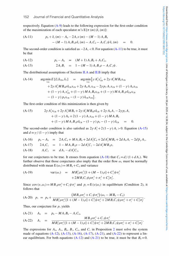
152 Journal of Financial and Quantitative Analysis
respectively. Equation (A-9) leads to the following expression for the first-order conditionof the maximization of each speculator m’s E[π (m) |δv (m)]:
p0+ δv (m)− A0− 2A1x (m)− (M − 1) A1 B0(A-11)
− (M − 1) A1 B1ρδv (m)− A1C0− A1C1ψδv (m) = 0.
The second-order condition is satisfied as−2A1<0. For equation (A-11) to be true, it mustbe that
p0− A0 = (M + 1) A1 B0+ A1C0,(A-12)
2A1 B1 = 1− (M − 1) A1 B1ρ− A1C1ψ.(A-13)
The distributional assumptions of Sections II.A and II.B imply that
argminxCB
E [L|δCB,δT ] = argminxCB
[γ A2
1x 2CB+ 2γ A2
1 M B0xCB(A-14)
+2γ A21 M B0ρδCBxCB+ 2γ A0 A1xCB− 2γ pT A1xCB+ (1− γ ) A0xCB
+ (1− γ ) A1x 2CB+ (1− γ )M A1 B0xCB+ (1− γ )M A1 B1ρδCBxCB
− (1− γ ) p0xCB− (1− γ )δCBxCB
].
The first-order condition of this minimization is then given by
2γ A21xCB+ 2γ A2
1 M B0+ 2γ A21 M B0ρδCB+ 2γ A0 A1− 2γ pT A1(A-15)
+ (1− γ ) A0+ 2(1− γ ) A1xCB+ (1− γ )M A1 B0
+ (1− γ )M A1 B1ρδCB− (1− γ ) p0− (1− γ )δCB = 0.
The second-order condition is also satisfied as 2γ A21+2(1−γ ) A1>0. Equation (A-15)
and d≡γ /(1−γ ) imply that
p0− A0 = 2A1C0+M A1 B0+ 2d A21C0+ 2d A2
1 M B0+ 2d A0 A1− 2d pT A1,(A-16)
2A1C1 = 1−M A1 B1ρ− 2d A21C1− 2d A2
1 M B1ρ,(A-17)
A1C2 = d A1− d A21C2,(A-18)
for our conjectures to be true. It ensues from equation (A-18) that C2=d/(1+d A1). Wefurther observe that those conjectures also imply that the order flow ω1 must be normallydistributed with mean E(ω1)=M B0+C0 and variance
var(ω1) = M B21ρσ
2v
[1+ (M − 1)ρ]+C 21ψσ
2v
(A-19)
+2M B1C1ψρσ2v+ σ 2
z +C 22σ
2T .
Since cov(v,ω1)=M B1ρσ2v+C1ψσ
2v
and p1=E(v|ω1) in equilibrium (Condition 2), itfollows that
(A-20) p1 = p0+
(M B1ρσ
2v+C1ψσ
2v
)(ω1−M B0−C0)
M B21ρσ
2v
[1+ (M − 1)ρ]+C 21ψσ
2v+ 2M B1C1ψρσ 2
v+ σ 2
z +C 22σ
2T
.
Thus, our conjecture for p1 yields
A0 = p0−M A1 B0− A1C0,(A-21)
A1 =M B1ρσ
2v+C1ψσ
2v
M B21ρσ
2v
[1+ (M − 1)ρ]+C 21ψσ
2v+ 2M B1C1ψρσ 2
v+ σ 2
z +C 22σ
2T
.(A-22)
The expressions for A0, A1, B0, B1, C0, and C1 in Proposition 2 must solve the systemmade of equations (A-12), (A-13), (A-16), (A-17), (A-21), and (A-22) to represent a lin-ear equilibrium. For both equations (A-12) and (A-21) to be true, it must be that B0=0.
https://doi.org/10.1017/S0022109018001552D
ownloaded from
https://ww
w.cam
bridge.org/core . Univ of M
ichigan Law Library , on 08 Jan 2020 at 16:38:34 , subject to the Cam
bridge Core terms of use, available at https://w
ww
.cambridge.org/core/term
s .

Pasquariello, Roush, and Vega 153
Defining A1C0= p0− A0 from equation (A-12) and plugging it into equation (A-16) leadsus to A0= p0+2d A1
(p0− pT
)and C0=2d
(pT − p0
). We are left with the task of finding
A1, B1, and C1. Solving equation (A-13) for B1 and equation (A-17) for C1 we get
B1 =1− A1C1ψ
A1 [2+ (M − 1)ρ],(A-23)
C1 =1−M A1 B1ρ (1+ 2d A1)
2A1 (1+ d A1),(A-24)
respectively. The system made of equations (A-23) and (A-24) implies that B1=
[2(1+d A1)−ψ]/[A1 f (A1)
]and C1={[2+(M−1)ρ]−Mρ (1+2d A1)}/
[A1 f (A1)
],
where f (A1)=2[2+(M−1)ρ](1+d A1)−Mψρ (1+2d A1). Next, we replace the pre-vious expressions for B1 and C1 in equation (A-22) to get the following sextic polynomialin A1,
(A-25) g6 A61+ g5 A5
1+ g4 A41+ g3 A3
1+ g2 A21+ g1 A1+ g0 = 0,
where it is a straightforward but tedious exercise to show that, for the parameter restrictionsin Sections II.A and II.B,
g0 = −σ 2v
[Mρ (2−ψ)2
+ψ (2− ρ)2]
< 0,(A-26)
g1 = −2σ 2vd{
Mρ[8− 6ψ −ψ 2 (1− ρ)
]+ 2ψ (2− ρ)2
}< 0,(A-27)
g2 = σ 2z Mρ
[Mρ (2−ψ)2
+ 4(2− ρ)(2−ψ)]
(A-28)
+σ 2T d2 [Mρ (2−ψ)+ 2(2− ρ)]2
+σ 2vd2{
Mρ[4Mρψ (1−ψ)+ψ 2 (7− 4ρ)+ 5ψ (4− ρ)− 24
]+ 5ψρ (4− ρ)− 20ψ
},
g3 = 2σ 2z d Mρ {Mρ [8−ψ (10− 3ψ)]+ 2[16− 5ψ (2− ρ)+ 8ρ]}(A-29)
+2σ 2vd3{4M 2ρ2ψ (1−ψ)+ 2Mρ
[ψ 2 (1− ρ)
+ ψ (5− 2ρ)− 4]−ψ (2− ρ)2
}+4σ 2
T d3{
M 2ρ2 [2−ψ (3−ψ)]
+ Mρ [8− 3ψ (2− ρ)− 4ρ]+ 2(2− ρ)2}
,
g4 = 4σ 2T d4 [Mρ (1−ψ)+ (2− ρ)]2(A-30)
+4σ 2vd4 Mρ [Mρψ (1−ψ)+ψ (2− ρ)− 1]
+σ 2z d2
{M 2ρ2 [24+ψ (13ψ − 36)]
+ 12Mρ [8− 3ψ (2− ρ)− 4ρ]+ 24(2− ρ)2}
,
g5 = 4σ 2z d3
{M 2ρ2 [4−ψ (7− 3ψ)](A-31)
+ Mρ [16− 7ψ (2− ρ)− 8ρ]+ 4(2− ρ)2}
> 0,
(A-32) g6 = 4σ 2z d4 [Mρ (1−ψ)+ (2− ρ)]2
> 0,
as well as (by numerical inspection) that sign(g3)=sign(g2)=sign(g1) and sign(g4)=
sign(g5), sign(g4)=sign(g3)=sign(g2), or sign(g3)=sign(g4)=sign(g5) and sign(g2)=
sign(g1) (i.e., that only one change of sign is possible while proceeding from the lowest tothe highest power). Descartes’ Rule then implies that the polynomial of equation (A-25)has only one positive real root satisfying the second-order conditions for both the specula-tors’ and the central bank’s optimization problems. This root, λCB, is therefore the uniquelinear Bayesian Nash equilibrium of the amended economy of Section II.B. According to
https://doi.org/10.1017/S0022109018001552D
ownloaded from
https://ww
w.cam
bridge.org/core . Univ of M
ichigan Law Library , on 08 Jan 2020 at 16:38:34 , subject to the Cam
bridge Core terms of use, available at https://w
ww
.cambridge.org/core/term
s .

154 Journal of Financial and Quantitative Analysis
Abel’s Impossibility Theorem, the polynomial of equation (A-25) cannot be solved withrational operations and finite root extractions. In the numerical examples of Figure 1, wefind λCB using the 3-stage algorithm proposed by Jenkins and Traub (1970a), (1970b). Un-fortunately, this algorithm does not always identify all roots of the polynomial of equation(A-25). Thus, those examples are based on exogenous parameter values such that λCB canbe found. For instance, this is the case under most model parameterizations when the cen-tral bank is nontrivially concerned about the cost of pursuing its uninformative policy targetpT (i.e., γ is sufficiently lower than 1). �
Supplementary MaterialSupplementary Material for this article is available at https://doi.org/10.1017/
S0022109018001552.
ReferencesAcharya, V., and M. Richardson (eds.), Restoring Financial Stability: How to Repair a Failed System—
An Independent View from New York University Stern School of Business, John Wiley & Sons(2009).
Afonso, G.; A. Kovner; and A. Schoar. “Stressed, Not Frozen: The Federal Funds Market in the Fi-nancial Crisis.” Journal of Finance, 66 (2011), 1109–1139.
Akhtar, M. “Understanding Open Market Operations.” Federal Reserve Bank of New York, PublicInformation Department (1997).
Andersen, T., and T. Bollerslev. “Deutsche Mark-Dollar Volatility: Intraday Activity Patterns, Macroe-conomic Announcements, and Longer Run Dependencies.” Journal of Finance, 53 (1998),219–265.
Andersen, T.; T. Bollerslev; F. Diebold; and C. Vega. “Micro Effects of Macro Announcements: Real-Time Price Discovery in Foreign Exchange.” American Economic Review, 93 (2003), 38–62.
Andersen, T.; T. Bollerslev; F. Diebold; and C. Vega. “Real-Time Price Discovery in Stock, Bond, andForeign Exchange Markets.” Journal of International Economics, 73 (2007), 251–277.
Bernanke, B., and K. Kuttner. “What Explains the Stock Market’s Reaction to Federal Reserve Pol-icy?” Journal of Finance, 60 (2005), 1221–1257.
Bhattacharya, U., and P. Weller. “The Advantage of Hiding One’s Hand: Speculation and CentralBank Intervention in the Foreign Exchange Market.” Journal of Monetary Economics, 39 (1997),251–277.
Bossaerts, P., and P. Hillion. “Market Microstructure Effects of Government Intervention in the For-eign Exchange Market.” Review of Financial Studies, 4 (1991), 513–541.
Brandt, M., and K. Kavajecz. “Price Discovery in the U.S. Treasury Market: The Impact of OrderFlow and Liquidity on the Yield Curve.” Journal of Finance, 59 (2004), 2623–2654.
Brenner, M.; P. Pasquariello; and M. Subrahmanyam. “On the Volatility and Comovement of U.S. Fi-nancial Markets around Macroeconomic News Announcements.” Journal of Financial and Quan-titative Analysis, 44 (2009), 1265–1289.
Caballe, J., and M. Krishnan. “Imperfect Competition in a Multi-Security Market with Risk Neutral-ity.” Econometrica, 62 (1994), 695–704.
Chari, A. “Heterogeneous Market-Making in Foreign Exchange Markets: Evidence from Individ-ual Bank Responses to Central Bank Interventions.” Journal of Money, Credit, and Banking, 39(2007), 1131–1161.
Chordia, T.; J. Hu; A. Subrahmanyam; and Q. Tong. “Order Flow Volatility and Equity Costs ofCapital.” Management Science, 65 (2019), 1520–1551.
Chordia, T.; A. Sarkar; and A. Subrahmanyam. “An Empirical Analysis of Stock and Bond MarketLiquidity.” Review of Financial Studies, 18 (2005), 85–129.
Chordia, T., and A. Subrahmanyam. “Order Imbalance and Individual Stock Returns: Theory andEvidence.” Journal of Financial Economics, 72 (2004), 485–518.
Christensen, J., and G. Rudebusch. “The Response of Interest Rates to U.S. and U.K. QuantitativeEasing.” Economic Journal, 122 (2012), 385–414.
Cieslak, A.; A. Morse; and A. Vissing-Jorgensen. “Stock Returns over the FOMC Cycle.” WorkingPaper, University of California-Berkeley (2016).
Cohen, B. “Monetary Policy Procedures and Volatility Transmission along the Yield Curve.” WorkingPaper, Bank for International Settlements (1999).
https://doi.org/10.1017/S0022109018001552D
ownloaded from
https://ww
w.cam
bridge.org/core . Univ of M
ichigan Law Library , on 08 Jan 2020 at 16:38:34 , subject to the Cam
bridge Core terms of use, available at https://w
ww
.cambridge.org/core/term
s .

Pasquariello, Roush, and Vega 155
Croushore, D. “Introducing: The Survey of Professional Forecasters.” Business Review, Federal Re-serve Bank of Philadelphia (1993), 3–15.
D’Amico, S.; W. English; D. Lopez-Salido; and E. Nelson. “The Federal Reserve’s Large-Scale AssetPurchase Programs: Rationale and Effects.” Economic Journal, 122 (2012), 415–446.
D’Amico, S., and T. King. “Flow and Stock Effects of Large-Scale Treasury Purchases: Evidence onthe Importance of Local Supply.” Journal of Financial Economics, 108 (2013), 425–448.
Diether, K.; C. Malloy; and A. Scherbina. “Differences of Opinion and the Cross Section of StockReturns.” Journal of Finance, 57 (2002), 2113–2141.
Dominguez, K. “The Market Microstructure of Central Bank Intervention.” Journal of InternationalEconomics, 59 (2003), 25–45.
Dominguez, K. “When Do Central Bank Interventions Influence Intra-Daily and Longer-Term Ex-change Rate Movements?” Journal of International Money and Finance, 25 (2006), 1051–1071.
Edwards, C. “Open Market Operations in the 1990s.” Federal Reserve Bulletin, 83 (1997), 859–874.Eser, F., and B. Schwaab. “Evaluating the Impact of Unconventional Monetary Policy Measures:
Empirical Evidence from the ECB’s Securities Markets Programme.” Journal of Financial Eco-nomics, 119 (2016), 147–167.
Evans, M., and R. Lyons. “Order Flow and Exchange Rate Dynamics.” Journal of Political Economy,110 (2002), 170–180.
Evans, M., and R. Lyons. “Are Different-Currency Assets Imperfect Substitutes?” In Exchange RateEconomics: Where Do We Stand?, P. De Grauwe, ed. MIT Press (2005), 1–34.
Fabozzi, F., and M. Fleming. “U.S. Treasury and Agency Securities.” In The Handbook of FixedIncome Securities, F. Fabozzi, ed. New York, NY: McGraw Hill (2004), 229–250.
Federal Reserve Bank of New York (FRBNY). Domestic Open Market Operations during 2004. Fed-eral Reserve System Publication (2005).
Federal Reserve Bank of New York (FRBNY). Domestic Open Market Operations during 2007. Fed-eral Reserve System Publication (2008).
Federal Reserve Board of Governors (FRBG). The Federal Reserve System: Purposes and Functions.Federal Reserve System Publication (2005).
Fleming, M. “The Round-the-Clock Market of U.S. Treasury Securities.” Economic Policy Review,Federal Reserve Bank of New York, 3 (1997), 9–32.
Fleming, M. “Measuring Treasury Market Liquidity.” Economic Policy Review, Federal Reserve Bankof New York, 9 (2003) 83–108.
Fleming, M.; B. Mizrach; and G. Nguyen. “The Microstructure of a U.S. Treasury ECN: The Bro-kerTec Platform.” Journal of Financial Markets, 40 (2018), 2–22.
Foster, F., and S. Viswanathan. “Strategic Trading When Agents Forecast the Forecasts of Others.”Journal of Finance, 51 (1996), 1437–1478.
Furfine, C. “The Microstructure of the Federal Funds Market.” Financial Markets, Institutions & In-struments, 8 (1999), 24–44.
Gagnon, J.; M. Raskin; J. Remache; and B. Sack. “The Financial Market Effects of the FederalReserve’s Large-Scale Asset Purchases.” International Journal of Central Banking, 7 (2011),3–43.
George, T.; G. Kaul; and M. Nimalendran. “Estimation of the Bid–Ask Spread and Its Components:A New Approach.” Review of Financial Studies, 4 (1991), 623–656.
Gilbert, T.; C. Scotti; G. Strasser; and C. Vega. “Is the Intrinsic Value of a Macroeconomic NewsAnnouncement Related to Its Asset Price Impact?” Journal of Monetary Economics, 92 (2017),78–95.
Goldreich, D.; B. Hanke; and P. Nath. “The Price of Future Liquidity: Time-Varying Liquidity in theU.S. Treasury Market.” Review of Finance, 9 (2005), 1–32.
Green, C. “Economic News and the Impact of Trading on Bond Prices.” Journal of Finance, 59 (2004),1201–1233.
Greene, W. Econometric Analysis. Upper Saddle River, NJ: Prentice Hall (1997).Greenwood, R., and D. Vayanos. “Price Pressure in the Government Bond Market.” American Eco-
nomic Review: Papers and Proceedings, 100 (2010), 585–590.Hamilton, J., and C. Wu. “The Effectiveness of Alternative Monetary Policy Tools in a Zero Lower
Bound Environment.” Journal of Money, Credit, and Banking, 44 (2011), 3–46.Harvey, C., and R. Huang. “The Impact of the Federal Reserve Bank’s Open Market Operations.”
Journal of Financial Markets, 5 (2002), 223–257.Hasbrouck, J. “Measuring the Information Content of Stock Trades.” Journal of Finance, 46 (1991),
179–207.Hasbrouck, J. Empirical Market Microstructure. Oxford, UK: Oxford University Press (2007).Hu, X.; J. Pan; and J. Wang. “Noise as Information for Illiquidity.” Journal of Finance, 68 (2013),
2223–2772.
https://doi.org/10.1017/S0022109018001552D
ownloaded from
https://ww
w.cam
bridge.org/core . Univ of M
ichigan Law Library , on 08 Jan 2020 at 16:38:34 , subject to the Cam
bridge Core terms of use, available at https://w
ww
.cambridge.org/core/term
s .

156 Journal of Financial and Quantitative Analysis
Inoue, H. “The Effects of Open Market Operations on the Price Discovery Process in the JapaneseGovernment Securities Market: An Empirical Study.” Working Paper, Bank of Japan (1999).
Jenkins, M., and J. Traub. “A Three-Stage Variables-Shift Iteration for Polynomial Zeros and Its Re-lation to Generalized Rayleigh Iteration.” Numerishe Mathematik, 14 (1970a), 252–263.
Jenkins, M., and J. Traub. “A Three-Stage Algorithm for Real Polynomials Using Quadratic Iteration.”SIAM Journal of Numerical Analysis, 7 (1970b), 545–566.
Jones, C.; G. Kaul; and M. Lipson. “Transactions, Volume, and Volatility.” Review of Financial Stud-ies, 7 (1994), 631–651.
Kitsul, Y. “Large-Scale Asset Purchases and Liquidity of Treasury Securities.” Working Paper, FederalReserve Board of Governors (2013).
Krishnamurthy, A. “The Bond/Old-Bond Spread.” Journal of Financial Economics, 66 (2002),463–506.
Krishnamurthy, A.; S. Nagel; and A. Vissing-Jorgensen. “ECB Policies Involving Government BondPurchases: Impact and Channel.” Review of Finance, 22 (2018), 1–44.
Krishnamurthy, A., and A. Vissing-Jorgensen. “The Effects of Quantitative Easing on Interest Rates.”Brookings Papers on Economic Activity, (2011), 215–287.
Krishnamurthy, A., and A. Vissing-Jorgensen. “The Aggregate Demand for Treasury Debt.” Journalof Political Economy, 120 (2012), 233–267.
Kumar, P., and D. Seppi. “Futures Manipulation with ‘Cash Settlement’.” Journal of Finance, 47(1992), 1485–1502.
Kyle, A. “Continuous Auctions and Insider Trading.” Econometrica, 53 (1985), 1315–1335.Li, H.; J. Wang; C. Wu; and Y. He. “Are Liquidity and Information Risks Priced in the Treasury Bond
Market?” Journal of Finance, 64 (2009), 467–503.Lyons, R. The Microstructure Approach to Exchange Rates. Cambridge, MA: MIT Press (2001).Mizrach, B., and C. Neely. “The Transition to Electronic Communications Networks in the Secondary
Treasury Market.” Federal Reserve Bank of St. Louis Review, 88 (2006), 527–541.Mizrach, B., and C. Neely. “The Microstructure of the U.S. Treasury Market.” In Encyclopedia of
Complexity and Systems Science, R. Meyers, ed. Springer-Verlag (2009), 9565–9577.Naranjo, A., and M. Nimalendran. “Government Intervention and Adverse Selection Costs in Foreign
Exchange Markets.” Review of Financial Studies, 13 (2000), 453–477.Neely, C. “Identifying the Effects of U.S. Intervention on the Levels of Exchange Rates.” Reserve
Bank of St. Louis Working Paper No. 2005-031C (2005).Novshek, W. “Finding All n-Firm Cournot Equilibria.” International Economic Review, 25 (1984),
61–70.O’Hara, M. Market Microstructure Theory. Cambridge, MA: Blackwell (1995).Pasquariello, P. “Imperfect Competition, Information Heterogeneity, and Financial Contagion.” Re-
view of Financial Studies, 20 (2007a), 391–426.Pasquariello, P. “Informative Trading or Just Costly Noise? An Analysis of Central Bank Interven-
tions.” Journal of Financial Markets, 10 (2007b), 107–143.Pasquariello, P. “Central Bank Intervention and the Intraday Process of Price Formation in the Cur-
rency Markets.” Journal of International Money and Finance, 29 (2010), 1045–1061.Pasquariello, P. “Government Intervention and Arbitrage.” Review of Financial Studies, 31 (2018),
3344–3408.Pasquariello, P., and C. Vega. “Informed and Strategic Order Flow in the Bond Markets.” Review of
Financial Studies, 20 (2007), 1975–2019.Pasquariello, P., and C. Vega. “The On-the-Run Liquidity Phenomenon.” Journal of Financial Eco-
nomics, 92 (2009), 1–24.Pasquariello, P., and C. Vega. “Strategic Cross-Trading in the U.S. Stock Market.” Review of Finance,
9 (2015), 229–282.Payne, R., and P. Vitale. “A Transaction Level Study of the Effects of Central Bank Intervention on
Exchange Rates.” Journal of International Economics, 61 (2003), 331–352.Sarno, L., and M. Taylor. “Official Intervention in the Foreign Exchange Market: Is It Effective, and
If So, How Does It Work?” Journal of Economic Literature, 39 (2001), 839–868.Sokolov, V. “The Impact of Open Market Operations on the Government Bond Market: Microstructure
Evidence.” Working Paper, Higher School of Economics (2009).Song, Z., and H. Zhu. “Quantitative Easing Auctions of Treasury Bonds.” Journal of Financial Eco-
nomics, 128 (2018), 103–124.Stein, J. “Cheap Talk and the Fed: A Theory of Imprecise Policy Announcements.” American Eco-
nomic Review, 79 (1989), 32–42.Stoll, H. “Inferring the Components of the Bid-Ask Spread: Theory and Empirical Tests.” Journal of
Finance, 44 (1989), 115–134.
https://doi.org/10.1017/S0022109018001552D
ownloaded from
https://ww
w.cam
bridge.org/core . Univ of M
ichigan Law Library , on 08 Jan 2020 at 16:38:34 , subject to the Cam
bridge Core terms of use, available at https://w
ww
.cambridge.org/core/term
s .

Pasquariello, Roush, and Vega 157
Strebulaev, I. “Liquidity and Asset Pricing: Evidence from the U.S. Treasury Securities Market.”Working Paper, London Business School (2002).
Vayanos, D., and J. Vila. “A Preferred-Habitat Model of the Term Structure of Interest Rates.” NBERWorking Paper No. 15487 (2009).
Vitale, P. “Sterilised Central Bank Intervention in the Foreign Exchange Market.” Journal of Interna-tional Economics, 49 (1999), 245–267.
Yu, J. “Disagreement and Return Predictability of Stock Portfolios.” Journal of Financial Economics,99 (2011), 162–183.
https://doi.org/10.1017/S0022109018001552D
ownloaded from
https://ww
w.cam
bridge.org/core . Univ of M
ichigan Law Library , on 08 Jan 2020 at 16:38:34 , subject to the Cam
bridge Core terms of use, available at https://w
ww
.cambridge.org/core/term
s .