grammar a disser - university of...
TRANSCRIPT
AUTOMATIC GRAMMAR GENERATION FROM TWO
DIFFERENT PERSPECTIVES
Fei Xia
A DISSERTATION
in
Computer and Information Science
Presented to the Faculties of the University of Pennsylvania
in Partial Ful�llment of the Requirements for the Degree of Doctor of Philosophy
2001
Professor Martha Palmer and Aravind JoshiSupervisors of Dissertation
Val TannenGraduate Group Chair

COPYRIGHT
Fei Xia
2001

To my family
iii

Acknowledgements
I thank everyone at the University of Pennsylvania (UPenn) and elsewhere who has helped
me to mature not only as a scientist but also as a human being.
I thank my advisors Martha Palmer and Aravind Joshi. Martha is not only a wonderful
mentor, but also a dear friend. Her steady support and encouragement helped me to go
through many diÆcult times. Dr. Joshi has always been my role model. He taught me to
trust myself and follow my heart.
I thank my dissertation committee members | ChuRen Huang from the Academia
Sinica in Taiwan, Vijay Shanker from the University of Delaware, Mitch Marcus, Steven
Bird, and Tony Kroch from UPenn | for their valuable suggestions and comments about
my thesis research. I would also like to thank Hiyan Alshawi from the AT&T Research
Lab for being a great mentor when I worked there as a summer intern.
I thank people at the Computer and Information Science Department (CIS) and the
Institute for Research in Cognitive Science (IRCS) at the University of Pennsylvania from
whom I have learned a lot about natural language processing, linguistics, psycholinguistics,
and more. This includes people in the XTAG group (Bangalore Srinivas, Christy Doran,
Beth Ann Hockey, Seth Kulick, Rajesh Bhatt, Rashmi Prasad, Carlos Prolo, Karin Kip-
per, William Schuler, Hoa Trang Dang, Alexandra Kinyon, Libin Shen, David Chiang),
CIS/IRCS faculty members (Bonnie Webber, Mark Steedman, Lyle Ungar, Scott Wein-
stein, Jean Gallier, Sampath Kannan, Insup Lee, Peter Buneman, Susan Davison, Val Tan-
nen, Carl Gunter, Dale Miller, Robin Clark, and Ellen Prince), students/alumni (Michael
Collins, Adwait Ratnaparkhi, Jason Eisner, Dan Melamed, Matthew Stone, Breck Bald-
win, Je� Raynar, Owen Rambow, Nobo Komagata, Jong Park, Joseph Rosenzweig, Tom
iv

Morton, Dan Bikel, Szuting Yi, Dimitris Samaras, Kyle Hart, Wenfei Fan, Hongliang Xie,
Jianping Shi, Liwei Zhao, Suejung Huh, Hee-Hwan Kwak, Peggi Li, Alexander Williams,
John Bell, and Allan Lee), visiting scholars and PostDocs (Michelle Strube, Paola Merlo,
Mark Dras, Mickey Chandrashekhar, and Shuly Wintner), and stu� members (Mike Felker,
Gail Shannon, Amy Dunn, Amy Deitz, Christine Metz, Laurel Sweeney, Ann Bies, Nicole
Bolden, Trisha Yannuzzi, and Jennifer MacDougall). I especially like to thank Anoop
Sarkar, Chunghye Han, Susan Converse, Tonia Bleam and Je�rey Lidz for their supports
and friendships.
I thank Nianwen Xue, Fu-Dong Chiou, Shizhe Huang, Zhibiao Wu, Shudong Huang,
John Kovarik, Mary Ellen Okurowski, James Huang, Shengli Feng, Andi Wu, Zhixing
Jiang, DeKai Wu, Jin Wang, Shiwen Yu, Huang Changning, and others for helping me
and my team to build the Chinese Penn Treebank. I especially thank Tony Kroch for
inspiring my love for linguistics.
I would like to thank my friends with whom I have spent time enjoying life itself. Spe-
cial thanks go to Xiaobai Wang, Zheng Xue, Mingkang Xu, Yujin Zhao, Yuanyuan Zhou,
Hong Jin, Zhijun Zhang, Zhijun Liu, Qin Lin, Aimin Sun, and Jin Yu.
Last, but not the least, I thank my family for supporting me all these years. I thank
my parents for their unconditional love and for letting me to pursue my dreams. I thank
my two sisters for supporting me in every stage of my life. I thank my kids for bringing
so much joy to my life. I especially thank my husband for showing me a totally di�erent
perspective of life and for making me a better person.
v

Abstract
AUTOMATIC GRAMMAR GENERATION FROM TWO DIFFERENT
PERSPECTIVES
Fei Xia
Supervisors: Professor Martha Palmer and Aravind Joshi
Grammars are valuable resources for natural language processing. We divide the pro-
cess of grammar development into three tasks: selecting a formalism, de�ning the proto-
types, and building a grammar for a particular human language. After a brief discussion
about the �rst two tasks, we focus on the third task. Traditionally, grammars are built
by hand and there are many problems with this approach. To address these problems,
we built two systems that automatically generate grammars. The �rst system (LexOrg)
solves two major problems in grammar development: namely, the redundancy caused by
the reuse of structures in a grammar and the lack of explicit generalizations over the
structures in a grammar. LexOrg takes several types of speci�cation as input and com-
bines them to automatically generate a grammar. The second system (LexTract) extracts
Lexicalized Tree Adjoining Grammars (LTAGs) and Context-free Grammars (CFGs) from
Treebanks, and builds derivation trees that can be used to train statistical LTAG parsers
directly. In addition to creating Treebank grammars and producing training materials for
parsers, LexTract is also used to evaluate the coverage of existing hand-crafted grammars,
to compare grammars for di�erent languages, to detect annotation errors in Treebanks,
and to test certain linguistic hypotheses. LexOrg and LexTract provide two di�erent per-
spectives on grammars. In LexOrg, elementary trees in an LTAG grammar are the result
vi

of combining language speci�cations such as tree descriptions. In LexTract, elementary
trees are building blocks of syntactic structures in a Treebank. LexOrg makes explicit the
language speci�cations that form elementary trees, whereas LexTract makes explicit the
elementary trees that form syntactic structures. The systems provide a rich set of tools
for language description and comparison that greatly enhances our ability to build and
maintain grammars and Treebanks e�ectively.
vii
Contents
Acknowledgements iv
Abstract vi
1 Introduction 1
1.1 Problems with the traditional approach . . . . . . . . . . . . . . . . . . . . 2
1.2 Our approach to grammar development . . . . . . . . . . . . . . . . . . . . 3
1.2.1 Task 1: selecting a formalism . . . . . . . . . . . . . . . . . . . . . . 3
1.2.2 Task 2: de�ning the prototypes . . . . . . . . . . . . . . . . . . . . . 5
1.2.3 Task 3: building a grammar for a human language . . . . . . . . . . 5
1.3 Chapter summaries . . . . . . . . . . . . . . . . . . . . . . . . . . . . . . . . 7
2 Overview of LTAG 10
2.1 Basics of the LTAG formalism . . . . . . . . . . . . . . . . . . . . . . . . . . 11
2.1.1 Elementary trees . . . . . . . . . . . . . . . . . . . . . . . . . . . . . 11
2.1.2 Two operations . . . . . . . . . . . . . . . . . . . . . . . . . . . . . . 11
2.1.3 Derived trees and derivation trees . . . . . . . . . . . . . . . . . . . 13
2.1.4 Multi-anchor trees . . . . . . . . . . . . . . . . . . . . . . . . . . . . 13
2.1.5 Feature structures . . . . . . . . . . . . . . . . . . . . . . . . . . . . 15
2.2 LTAG for natural languages . . . . . . . . . . . . . . . . . . . . . . . . . . . 16
2.3 Multi-component TAGs (MCTAGs) . . . . . . . . . . . . . . . . . . . . . . 18
2.4 Components of LTAG grammars for natural languages . . . . . . . . . . . . 20
2.4.1 An LTAG grammar is divided into a set of templates and a lexicon . 20
viii

2.4.2 A lexicon is split into a syntactic database and a morphological
database . . . . . . . . . . . . . . . . . . . . . . . . . . . . . . . . . . 22
2.4.3 Templates are grouped into tree families . . . . . . . . . . . . . . . . 23
2.5 The XTAG grammar . . . . . . . . . . . . . . . . . . . . . . . . . . . . . . . 24
2.6 Summary . . . . . . . . . . . . . . . . . . . . . . . . . . . . . . . . . . . . . 25
3 The target grammars 26
3.1 Four types of structural information . . . . . . . . . . . . . . . . . . . . . . 26
3.1.1 Head and its projections . . . . . . . . . . . . . . . . . . . . . . . . . 27
3.1.2 Arguments of a head . . . . . . . . . . . . . . . . . . . . . . . . . . . 28
3.1.3 Modi�ers of a head . . . . . . . . . . . . . . . . . . . . . . . . . . . . 29
3.1.4 Syntactic variations . . . . . . . . . . . . . . . . . . . . . . . . . . . 29
3.2 The prototypes of the target grammars . . . . . . . . . . . . . . . . . . . . . 29
3.3 GTable: a grammar generated from three tables . . . . . . . . . . . . . . . . 32
3.4 The problems with GTable . . . . . . . . . . . . . . . . . . . . . . . . . . . . 35
3.5 Two approaches . . . . . . . . . . . . . . . . . . . . . . . . . . . . . . . . . . 38
3.5.1 LexOrg: building grammars from descriptions . . . . . . . . . . . . . 39
3.5.2 LexTract: extracting grammars from Treebanks . . . . . . . . . . . . 40
3.6 Summary . . . . . . . . . . . . . . . . . . . . . . . . . . . . . . . . . . . . . 41
4 LexOrg: a system that builds LTAGs from descriptions 42
4.1 Structure sharing among templates . . . . . . . . . . . . . . . . . . . . . . . 43
4.2 The overall approach of LexOrg . . . . . . . . . . . . . . . . . . . . . . . . . 44
4.3 The de�nition of a description . . . . . . . . . . . . . . . . . . . . . . . . . . 46
4.3.1 A compact representation of LTAG grammars . . . . . . . . . . . . . 46
4.3.2 The previous de�nition of description . . . . . . . . . . . . . . . . . 49
4.3.3 The de�nition of descriptions in LexOrg . . . . . . . . . . . . . . . . 51
4.4 The types of descriptions . . . . . . . . . . . . . . . . . . . . . . . . . . . . 55
4.4.1 Head and its projections . . . . . . . . . . . . . . . . . . . . . . . . . 56
4.4.2 Arguments of a head . . . . . . . . . . . . . . . . . . . . . . . . . . . 57
4.4.3 Modi�ers of a head . . . . . . . . . . . . . . . . . . . . . . . . . . . . 57
ix

4.4.4 Syntactic variations . . . . . . . . . . . . . . . . . . . . . . . . . . . 58
4.5 The Tree Generator . . . . . . . . . . . . . . . . . . . . . . . . . . . . . . . 59
4.5.1 Step 1: Combine descriptions to form a new description . . . . . . . 59
4.5.2 Step 2: Generate a set of trees from the new description . . . . . . . 61
4.5.3 Step 3: Build templates from the trees . . . . . . . . . . . . . . . . . 67
4.6 The Description Selector . . . . . . . . . . . . . . . . . . . . . . . . . . . . . 68
4.6.1 The function of the Description Selector . . . . . . . . . . . . . . . . 68
4.6.2 The de�nition of a subcategorization frame . . . . . . . . . . . . . . 70
4.6.3 The algorithm for the Description Selector . . . . . . . . . . . . . . . 72
4.7 The Frame Generator . . . . . . . . . . . . . . . . . . . . . . . . . . . . . . 74
4.7.1 The function of the Frame Generator . . . . . . . . . . . . . . . . . . 75
4.7.2 The de�nition of a lexical rule . . . . . . . . . . . . . . . . . . . . . 76
4.7.3 The algorithm for the Frame Generator . . . . . . . . . . . . . . . . 76
4.8 The experiments . . . . . . . . . . . . . . . . . . . . . . . . . . . . . . . . . 77
4.9 Creating language-speci�c information . . . . . . . . . . . . . . . . . . . . . 79
4.9.1 Subcategorization frames and lexical rules . . . . . . . . . . . . . . . 79
4.9.2 Descriptions . . . . . . . . . . . . . . . . . . . . . . . . . . . . . . . . 80
4.10 Comparison with other work . . . . . . . . . . . . . . . . . . . . . . . . . . 83
4.10.1 Becker's HyTAG . . . . . . . . . . . . . . . . . . . . . . . . . . . . . 86
4.10.2 The DATR system . . . . . . . . . . . . . . . . . . . . . . . . . . . . 92
4.10.3 Candito's system . . . . . . . . . . . . . . . . . . . . . . . . . . . . . 95
4.11 Summary . . . . . . . . . . . . . . . . . . . . . . . . . . . . . . . . . . . . . 98
5 LexTract: a system that extracts LTAGs from Treebanks 100
5.1 Overview of the English Penn Treebank . . . . . . . . . . . . . . . . . . . . 101
5.2 Overall approach of LexTract . . . . . . . . . . . . . . . . . . . . . . . . . . 102
5.3 Three input tables to LexTract . . . . . . . . . . . . . . . . . . . . . . . . . 106
5.3.1 Head percolation table . . . . . . . . . . . . . . . . . . . . . . . . . . 106
5.3.2 Argument table . . . . . . . . . . . . . . . . . . . . . . . . . . . . . . 107
5.3.3 Tagset table . . . . . . . . . . . . . . . . . . . . . . . . . . . . . . . . 108
5.4 Extracting LTAG grammars from Treebanks . . . . . . . . . . . . . . . . . . 108
x

5.4.1 Stage 1: Converting ttrees into derived trees . . . . . . . . . . . . . . 109
5.4.2 Stage 2: Building etrees . . . . . . . . . . . . . . . . . . . . . . . . . 109
5.4.3 Uniqueness of decomposition . . . . . . . . . . . . . . . . . . . . . . 114
5.4.4 Relations between nodes in ttrees and etrees . . . . . . . . . . . . . . 118
5.5 Creating derivation trees . . . . . . . . . . . . . . . . . . . . . . . . . . . . . 118
5.6 Building multi-component tree sets . . . . . . . . . . . . . . . . . . . . . . . 122
5.7 Building context-free rules and sub-templates . . . . . . . . . . . . . . . . . 126
5.8 Some special cases . . . . . . . . . . . . . . . . . . . . . . . . . . . . . . . . 128
5.8.1 Coordination . . . . . . . . . . . . . . . . . . . . . . . . . . . . . . . 128
5.8.2 Empty categories . . . . . . . . . . . . . . . . . . . . . . . . . . . . . 129
5.8.3 Punctuation marks . . . . . . . . . . . . . . . . . . . . . . . . . . . . 131
5.8.4 Predicative auxiliary trees . . . . . . . . . . . . . . . . . . . . . . . . 134
5.9 Comparison with other work . . . . . . . . . . . . . . . . . . . . . . . . . . 136
5.9.1 CFG extraction algorithms . . . . . . . . . . . . . . . . . . . . . . . 136
5.9.2 LTAG extraction algorithms . . . . . . . . . . . . . . . . . . . . . . . 138
5.10 Summary . . . . . . . . . . . . . . . . . . . . . . . . . . . . . . . . . . . . . 140
6 Applications of LexTract 142
6.1 Treebank grammars as stand-alone grammars . . . . . . . . . . . . . . . . . 142
6.1.1 Two Treebank grammars for English . . . . . . . . . . . . . . . . . . 143
6.1.2 Coverage of a Treebank grammar . . . . . . . . . . . . . . . . . . . . 144
6.1.3 Quality of a Treebank grammar . . . . . . . . . . . . . . . . . . . . . 148
6.2 Treebank grammars combined with other grammars . . . . . . . . . . . . . 149
6.2.1 Methodology . . . . . . . . . . . . . . . . . . . . . . . . . . . . . . . 150
6.2.2 Stage 1: Extracting templates from Treebanks . . . . . . . . . . . . 151
6.2.3 Stage 2: Matching templates in the two grammars . . . . . . . . . . 151
6.2.4 Stage 3: Classifying unmatched templates . . . . . . . . . . . . . . . 154
6.2.5 Stage 4: Combining two grammars . . . . . . . . . . . . . . . . . . . 155
6.3 Comparison of Treebank grammars for di�erent languages . . . . . . . . . . 156
6.3.1 Three Treebanks for three languages . . . . . . . . . . . . . . . . . . 157
xi
6.3.2 Stage 1: Extracting Treebank grammars that are based on the same
tagset . . . . . . . . . . . . . . . . . . . . . . . . . . . . . . . . . . . 159
6.3.3 Stage 2: Matching templates . . . . . . . . . . . . . . . . . . . . . . 159
6.3.4 Stage 3: Classifying unmatched templates . . . . . . . . . . . . . . . 164
6.3.5 The next step . . . . . . . . . . . . . . . . . . . . . . . . . . . . . . . 166
6.4 Lexicons as training data for Supertaggers . . . . . . . . . . . . . . . . . . . 169
6.4.1 Overview of Supertaggers . . . . . . . . . . . . . . . . . . . . . . . . 169
6.4.2 Experiments on training and testing Supertaggers . . . . . . . . . . 171
6.5 Derivation trees as training data for statistical LTAG parsers . . . . . . . . 175
6.5.1 Overview of Sarkar's parser . . . . . . . . . . . . . . . . . . . . . . . 175
6.5.2 Adjustments to the Treebank grammars for parsing . . . . . . . . . 176
6.6 LexTract as a tool for error detection in Treebank annotation . . . . . . . . 177
6.6.1 Algorithm for error detection . . . . . . . . . . . . . . . . . . . . . . 177
6.6.2 Types of error that LexTract detects . . . . . . . . . . . . . . . . . . 178
6.6.3 Experimental results . . . . . . . . . . . . . . . . . . . . . . . . . . . 182
6.7 MC sets for testing the Tree-locality Hypothesis . . . . . . . . . . . . . . . . 183
6.7.1 Stage 1: Finding \non-local" examples . . . . . . . . . . . . . . . . . 183
6.7.2 Stage 2: Classifying \non-local" examples . . . . . . . . . . . . . . . 183
6.7.3 Stage 3: Studying \non-local" constructions . . . . . . . . . . . . . . 185
6.8 Summary . . . . . . . . . . . . . . . . . . . . . . . . . . . . . . . . . . . . . 189
7 Phrase structures and dependency structures 191
7.1 Dependency structures . . . . . . . . . . . . . . . . . . . . . . . . . . . . . . 192
7.2 Converting phrase structures to dependency structures . . . . . . . . . . . . 194
7.3 Converting dependency structures to phrase structures . . . . . . . . . . . . 196
7.3.1 Algorithm 1 . . . . . . . . . . . . . . . . . . . . . . . . . . . . . . . . 197
7.3.2 Algorithm 2 . . . . . . . . . . . . . . . . . . . . . . . . . . . . . . . . 198
7.3.3 Algorithm 3 . . . . . . . . . . . . . . . . . . . . . . . . . . . . . . . . 199
7.3.4 Algorithm 1 and 2 as special cases of Algorithm 3 . . . . . . . . . . 206
7.4 Experiments . . . . . . . . . . . . . . . . . . . . . . . . . . . . . . . . . . . . 210
7.5 Discussion . . . . . . . . . . . . . . . . . . . . . . . . . . . . . . . . . . . . . 212
xii
7.5.1 Extending Algorithm 3 . . . . . . . . . . . . . . . . . . . . . . . . . 212
7.5.2 Empty categories in dependency structures . . . . . . . . . . . . . . 213
7.5.3 Running LexTract on a dependency Treebank . . . . . . . . . . . . . 213
7.6 Summary . . . . . . . . . . . . . . . . . . . . . . . . . . . . . . . . . . . . . 217
8 Conclusion 219
8.1 Contributions . . . . . . . . . . . . . . . . . . . . . . . . . . . . . . . . . . . 219
8.1.1 The prototypes of elementary trees . . . . . . . . . . . . . . . . . . . 219
8.1.2 LexOrg: a system that generates grammars from descriptions . . . . 220
8.1.3 LexTract: a system that extracts grammars from Treebanks . . . . . 221
8.1.4 The role of linguistic experts in grammar development . . . . . . . . 223
8.1.5 Relationship between two types of syntactic representation . . . . . 224
8.2 Future work . . . . . . . . . . . . . . . . . . . . . . . . . . . . . . . . . . . . 224
8.2.1 Combining the strengths of LexOrg and LexTract . . . . . . . . . . 225
8.2.2 Building and using parallel Treebanks . . . . . . . . . . . . . . . . . 226
A Language-speci�c tables 229
A.1 The formats of the language-speci�c tables . . . . . . . . . . . . . . . . . . 229
A.1.1 Tagset table . . . . . . . . . . . . . . . . . . . . . . . . . . . . . . . . 230
A.1.2 Head percolation table . . . . . . . . . . . . . . . . . . . . . . . . . . 230
A.1.3 Argument table . . . . . . . . . . . . . . . . . . . . . . . . . . . . . . 231
A.1.4 Modi�cation table . . . . . . . . . . . . . . . . . . . . . . . . . . . . 232
A.1.5 Head projection table . . . . . . . . . . . . . . . . . . . . . . . . . . 232
A.2 Tables for the English Penn Treebank . . . . . . . . . . . . . . . . . . . . . 232
A.2.1 Tagset table . . . . . . . . . . . . . . . . . . . . . . . . . . . . . . . . 232
A.2.2 Head percolation table . . . . . . . . . . . . . . . . . . . . . . . . . . 237
A.2.3 Argument table . . . . . . . . . . . . . . . . . . . . . . . . . . . . . . 238
A.2.4 Modi�cation table . . . . . . . . . . . . . . . . . . . . . . . . . . . . 238
A.2.5 Head projection table . . . . . . . . . . . . . . . . . . . . . . . . . . 239
A.3 Tables for the Chinese Penn Treebank . . . . . . . . . . . . . . . . . . . . . 241
A.3.1 Tagset table . . . . . . . . . . . . . . . . . . . . . . . . . . . . . . . . 241
xiii
A.3.2 Head percolation table . . . . . . . . . . . . . . . . . . . . . . . . . . 244
A.3.3 Argument table . . . . . . . . . . . . . . . . . . . . . . . . . . . . . . 245
A.4 Tables for the Korean Penn Treebank . . . . . . . . . . . . . . . . . . . . . 246
A.4.1 Tagset table . . . . . . . . . . . . . . . . . . . . . . . . . . . . . . . . 246
A.4.2 Head percolation table . . . . . . . . . . . . . . . . . . . . . . . . . . 248
A.4.3 Argument table . . . . . . . . . . . . . . . . . . . . . . . . . . . . . . 248
B Building a high-quality Treebank 250
B.1 Overview of the Chinese Penn Treebank Project . . . . . . . . . . . . . . . 251
B.1.1 Project inception . . . . . . . . . . . . . . . . . . . . . . . . . . . . . 252
B.1.2 Annotation process . . . . . . . . . . . . . . . . . . . . . . . . . . . . 253
B.2 Methodology for guideline preparation . . . . . . . . . . . . . . . . . . . . . 254
B.3 Segmentation guidelines . . . . . . . . . . . . . . . . . . . . . . . . . . . . . 256
B.3.1 Notions of word . . . . . . . . . . . . . . . . . . . . . . . . . . . . . . 256
B.3.2 An experiment . . . . . . . . . . . . . . . . . . . . . . . . . . . . . . 258
B.3.3 Tests of wordness . . . . . . . . . . . . . . . . . . . . . . . . . . . . . 260
B.4 POS tagging guidelines . . . . . . . . . . . . . . . . . . . . . . . . . . . . . . 262
B.4.1 Criteria for POS tagging . . . . . . . . . . . . . . . . . . . . . . . . . 262
B.4.2 Choice of a POS tagset . . . . . . . . . . . . . . . . . . . . . . . . . 263
B.5 Syntactic bracketing guidelines . . . . . . . . . . . . . . . . . . . . . . . . . 265
B.5.1 Representation scheme . . . . . . . . . . . . . . . . . . . . . . . . . . 265
B.5.2 Syntactic constructions . . . . . . . . . . . . . . . . . . . . . . . . . 267
B.5.3 Ambiguities . . . . . . . . . . . . . . . . . . . . . . . . . . . . . . . . 268
B.6 Quality control . . . . . . . . . . . . . . . . . . . . . . . . . . . . . . . . . . 269
B.6.1 Two passes in each phase . . . . . . . . . . . . . . . . . . . . . . . . 269
B.6.2 Double re-annotation in the bracketing phase . . . . . . . . . . . . . 269
B.6.3 Error detection using LexTract . . . . . . . . . . . . . . . . . . . . . 270
B.7 The role of NLP tools . . . . . . . . . . . . . . . . . . . . . . . . . . . . . . 271
B.7.1 Preprocessing tools . . . . . . . . . . . . . . . . . . . . . . . . . . . . 271
B.7.2 Annotation and conversion tools . . . . . . . . . . . . . . . . . . . . 272
B.7.3 Corpus search tools . . . . . . . . . . . . . . . . . . . . . . . . . . . 272
xiv
B.7.4 Quality-control tools . . . . . . . . . . . . . . . . . . . . . . . . . . . 273
B.8 Treebank guidelines and hand-crafted grammars . . . . . . . . . . . . . . . 273
B.9 Summary . . . . . . . . . . . . . . . . . . . . . . . . . . . . . . . . . . . . . 274
Bibliography 275
xv
List of Tables
1.1 The comparison between three approaches for grammar development . . . . 7
3.1 An algorithm that builds templates using three tables . . . . . . . . . . . . 34
4.1 The de�nition of a description given in (Rogers & Vijay-shanker, 1994) . . . 49
4.2 The de�nition of a tree given in (Rogers & Vijay-shanker, 1994) . . . . . . . 50
4.3 The new de�nition of description used in LexOrg . . . . . . . . . . . . . . . 52
4.4 The new de�nition of tree used in LexOrg . . . . . . . . . . . . . . . . . . . 53
4.5 A naive algorithm for buildingModmin(�) . . . . . . . . . . . . . . . . . . . 62
4.6 A revised version of the naive algorithm for building Modmin(�) . . . . . . 63
4.7 A much more eÆcient algorithm for building Modmin(�) . . . . . . . . . . . 64
4.8 An algorithm that builds a template from a tree . . . . . . . . . . . . . . . 69
4.9 The algorithm for the Description Selector . . . . . . . . . . . . . . . . . . . 73
4.10 Some examples of subcategorization frames, lexical rules, and descriptions
for English and Chinese . . . . . . . . . . . . . . . . . . . . . . . . . . . . . 79
4.11 The similarities and the di�erences between metarules, lexical rules, and
descriptions . . . . . . . . . . . . . . . . . . . . . . . . . . . . . . . . . . . . 89
5.1 Treebank tags that appear in this chapter . . . . . . . . . . . . . . . . . . . 102
5.2 Algorithm for �nding head-child of a node . . . . . . . . . . . . . . . . . . . 110
5.3 Algorithm that marks a node as either an argument or an adjunct . . . . . 111
5.4 Algorithm for building a derived tree . . . . . . . . . . . . . . . . . . . . . . 112
5.5 Algorithm for building etrees from a derived tree . . . . . . . . . . . . . . . 115
5.6 The bidirectional function between nodes in ttrees and etrees . . . . . . . . 118
xvi
5.7 Algorithm for building derivation trees . . . . . . . . . . . . . . . . . . . . . 121
5.8 Algorithm for building MC sets and testing whether the coindexation be-
tween a pair of nodes is tree-local . . . . . . . . . . . . . . . . . . . . . . . . 125
6.1 The tags in the PTB that are merged to a single tag in the XTAG grammar
and in G2 . . . . . . . . . . . . . . . . . . . . . . . . . . . . . . . . . . . . . 143
6.2 Two LTAG grammars extracted from the PTB . . . . . . . . . . . . . . . . 143
6.3 The types of unknown (word, template) pairs in Section 23 of the PTB . . 147
6.4 The numbers of templates in G1 and G2 with the threshold set to various
values . . . . . . . . . . . . . . . . . . . . . . . . . . . . . . . . . . . . . . . 148
6.5 Matched templates and their coverage . . . . . . . . . . . . . . . . . . . . . 153
6.6 Matched templates when certain annotation di�erences are disregarded . . 154
6.7 Classi�cation of 289 unmatched templates . . . . . . . . . . . . . . . . . . . 155
6.8 Sizes of the Treebanks and their tagsets . . . . . . . . . . . . . . . . . . . . 158
6.9 Grammars extracted from the three Treebanks . . . . . . . . . . . . . . . . 158
6.10 Treebank grammars with the new tagset . . . . . . . . . . . . . . . . . . . . 159
6.11 Numbers of matched templates, context-free rules, and sub-templates in
three grammar pairs . . . . . . . . . . . . . . . . . . . . . . . . . . . . . . . 161
6.12 The numbers of templates in the Treebank grammars with the threshold set
to various values . . . . . . . . . . . . . . . . . . . . . . . . . . . . . . . . . 162
6.13 Matched templates in the Treebank grammars with various threshold values 163
6.14 The distribution of the Chinese templates that do not match any English
templates . . . . . . . . . . . . . . . . . . . . . . . . . . . . . . . . . . . . . 166
6.15 The top 40 words with highest numbers of Supertags in G2 . . . . . . . . . 172
6.16 Supertagging results based on three di�erent conversion algorithms . . . . . 174
6.17 Algorithm for error detection . . . . . . . . . . . . . . . . . . . . . . . . . . 178
6.18 Numbers of tree sets and their frequencies in the PTB . . . . . . . . . . . . 183
6.19 Classi�cation of 999 MC sets that look non-tree-local . . . . . . . . . . . . . 184
7.1 Algorithm 3 for converting d-trees to phrase structures . . . . . . . . . . . . 203
xvii
7.2 Algorithm for attaching the phrase structure for the dependent to that for
the head . . . . . . . . . . . . . . . . . . . . . . . . . . . . . . . . . . . . . . 204
7.3 Algorithm for handling Chomsky modi�ers . . . . . . . . . . . . . . . . . . 207
7.4 Algorithm for moving up conjunctions . . . . . . . . . . . . . . . . . . . . . 207
7.5 Algorithm for attaching punctuation marks to phrase structures . . . . . . 208
7.6 The complete Algorithm 3 for converting d-tree to phrase structure . . . . . 208
7.7 Performance of three conversion algorithms on Section 0 of the PTB . . . . 211
7.8 Some examples of heads with more than one projection chain . . . . . . . . 212
7.9 Algorithm for building elementary trees directly from a d-tree . . . . . . . . 215
7.10 Algorithm for updating the elementary trees for the head and the dependent 216
8.1 The comparison between three approaches for grammar development . . . . 220
B.1 Comparison of word segmentation results from seven groups . . . . . . . . . 259
B.2 The process of creating and revising POS guidelines . . . . . . . . . . . . . 266
xviii
List of Figures
1.1 Combining elementary trees to generate a parse tree for a sentence . . . . . 4
1.2 Three prototypes of elementary trees in the target grammars . . . . . . . . 5
1.3 The organization of the dissertation . . . . . . . . . . . . . . . . . . . . . . 8
2.1 The substitution operation . . . . . . . . . . . . . . . . . . . . . . . . . . . 12
2.2 The adjoining operation . . . . . . . . . . . . . . . . . . . . . . . . . . . . . 12
2.3 Elementary trees, derived tree and derivation tree for underwriters still draft
policies. . . . . . . . . . . . . . . . . . . . . . . . . . . . . . . . . . . . . . . 13
2.4 Two derivation trees for a derived tree . . . . . . . . . . . . . . . . . . . . . 14
2.5 Multi-anchor trees . . . . . . . . . . . . . . . . . . . . . . . . . . . . . . . . 14
2.6 The substitution operation with features . . . . . . . . . . . . . . . . . . . . 15
2.7 The adjoining operation with features . . . . . . . . . . . . . . . . . . . . . 15
2.8 Features for the subject-verb agreement . . . . . . . . . . . . . . . . . . . . 16
2.9 An LTAG grammar that generates the language fanbncndng . . . . . . . . . 16
2.10 Cross-serial dependencies in Dutch . . . . . . . . . . . . . . . . . . . . . . . 18
2.11 Trees for the wh-question What does John like . . . . . . . . . . . . . . . . 19
2.12 Trees for the wh-question What does Mary think Mike believes John likes . 19
2.13 Tree-local MCTAG . . . . . . . . . . . . . . . . . . . . . . . . . . . . . . . . 20
2.14 An elementary tree is equivalent to a (word, template) pair . . . . . . . . . 21
2.15 A set of elementary trees is equivalent to a set of templates plus a lexicon . 21
2.16 A lexicon is split into two databases . . . . . . . . . . . . . . . . . . . . . . 22
2.17 A tree family . . . . . . . . . . . . . . . . . . . . . . . . . . . . . . . . . . . 23
2.18 The components of an LTAG grammar . . . . . . . . . . . . . . . . . . . . . 24
xix
3.1 The notions of head in X-bar theory and GB-theory . . . . . . . . . . . . . 28
3.2 Four templates in the transitive tree family . . . . . . . . . . . . . . . . . . 28
3.3 The three forms of elementary trees in the target grammar . . . . . . . . . 30
3.4 A spine-etree in which an argument is further expanded . . . . . . . . . . . 31
3.5 A spine-etree which is also an auxiliary tree . . . . . . . . . . . . . . . . . . 32
3.6 An example that shows the input and the output of the algorithm in Table
3.1 . . . . . . . . . . . . . . . . . . . . . . . . . . . . . . . . . . . . . . . . . 36
3.7 Among four of the templates in GTable for ditransitive verbs, the last two
are implausible. . . . . . . . . . . . . . . . . . . . . . . . . . . . . . . . . . . 37
3.8 Among four of the templates in GTable for relative clauses, the last two are
implausible. . . . . . . . . . . . . . . . . . . . . . . . . . . . . . . . . . . . . 38
3.9 The algorithm that generates grammars from tables alone . . . . . . . . . . 39
3.10 The input and output of LexOrg . . . . . . . . . . . . . . . . . . . . . . . . 39
3.11 Tree description for a relative clause . . . . . . . . . . . . . . . . . . . . . . 40
3.12 The conceptual approach of LexTract . . . . . . . . . . . . . . . . . . . . . 40
3.13 The relations between GTable, GL and G�Table . . . . . . . . . . . . . . . . . 41
4.1 Templates in two tree families . . . . . . . . . . . . . . . . . . . . . . . . . . 43
4.2 Structures shared by the templates in Figure 4.1 . . . . . . . . . . . . . . . 44
4.3 Combining descriptions to generate templates . . . . . . . . . . . . . . . . . 45
4.4 The architecture of LexOrg . . . . . . . . . . . . . . . . . . . . . . . . . . . 45
4.5 The fragment of the lexicon given in (Vijay-shanker & Schabes, 1992) . . . 47
4.6 The de�nition of six verb classes given in (Vijay-shanker & Schabes, 1992) . 47
4.7 Rules to handle wh-movement and passive . . . . . . . . . . . . . . . . . . . 48
4.8 A description and two templates that subsume it . . . . . . . . . . . . . . . 49
4.9 Two representations of a description . . . . . . . . . . . . . . . . . . . . . . 52
4.10 Two representations of a tree . . . . . . . . . . . . . . . . . . . . . . . . . . 55
4.11 A tree and the template that is built from the tree . . . . . . . . . . . . . . 56
4.12 Two sets of descriptions that generate the same tree . . . . . . . . . . . . . 57
4.13 Subcategorization descriptions . . . . . . . . . . . . . . . . . . . . . . . . . 58
4.14 A description for purpose clauses . . . . . . . . . . . . . . . . . . . . . . . . 58
xx

4.15 A description for wh-movement . . . . . . . . . . . . . . . . . . . . . . . . . 59
4.16 The function of the Tree Generator . . . . . . . . . . . . . . . . . . . . . . . 60
4.17 An example that illustrates how the new algorithm works . . . . . . . . . . 65
4.18 A tree and the template built from it . . . . . . . . . . . . . . . . . . . . . . 68
4.19 The function of the Tree Generator . . . . . . . . . . . . . . . . . . . . . . . 70
4.20 The function of the Description Selector . . . . . . . . . . . . . . . . . . . . 71
4.21 Templates in two tree families . . . . . . . . . . . . . . . . . . . . . . . . . . 75
4.22 The lexical rule for the causative/inchoative alternation . . . . . . . . . . . 75
4.23 The architecture of LexOrg . . . . . . . . . . . . . . . . . . . . . . . . . . . 78
4.24 A template and a set of descriptions that can generate it . . . . . . . . . . . 81
4.25 A more desirable description set if the template is for English . . . . . . . . 81
4.26 Descriptions built from language-speci�c tables . . . . . . . . . . . . . . . . 83
4.27 A description for wh-movement . . . . . . . . . . . . . . . . . . . . . . . . . 84
4.28 The lexical hierarchy given in (Vijay-Shanker & Schabes, 1992) . . . . . . . 85
4.29 A di�erent hierarchy for English verb classes . . . . . . . . . . . . . . . . . 85
4.30 Applying metarules to templates . . . . . . . . . . . . . . . . . . . . . . . . 87
4.31 The result of applying a metarule to a template may not be unique . . . . . 88
4.32 The ways that templates in a tree family are related in two systems . . . . 91
4.33 The ways that templates in di�erent tree families are related in two systems 92
4.34 An elementary tree and its DATR representation . . . . . . . . . . . . . . . 92
4.35 The principal lexical hierarchy and the de�nitions of two classes which are
given in (Evans et. al., 1995) . . . . . . . . . . . . . . . . . . . . . . . . . . 93
4.36 The lexical rules for topicalization, wh-movement, and passive in the DATR
system . . . . . . . . . . . . . . . . . . . . . . . . . . . . . . . . . . . . . . . 94
4.37 The di�erent ways that two systems handle wh-movement . . . . . . . . . . 98
5.1 Architecture of LexTract . . . . . . . . . . . . . . . . . . . . . . . . . . . . . 101
5.2 The Treebank annotation for the sentence Supply troubles were on the minds
of Treasury investors yesterday, who worried about the ood. . . . . . . . . . 103
5.3 The conceptual approach of LexTract . . . . . . . . . . . . . . . . . . . . . 103
5.4 The real implementation of LexTract . . . . . . . . . . . . . . . . . . . . . . 105
xxi
5.5 Two LTAG grammars that generate the same ttree . . . . . . . . . . . . . . 105
5.6 The percolation of lexical items from heads to higher projections . . . . . . 107
5.7 A ttree and the derived tree . . . . . . . . . . . . . . . . . . . . . . . . . . . 110
5.8 The etree set is a decomposition of the derived tree. . . . . . . . . . . . . . 114
5.9 The extracted etrees from the derived tree. . . . . . . . . . . . . . . . . . . 116
5.10 Several tree sets for a derived tree . . . . . . . . . . . . . . . . . . . . . . . 117
5.11 An example of the bidirectional function between nodes in ttrees and etrees 119
5.12 LTAG derivation trees for the sentence . . . . . . . . . . . . . . . . . . . . . 120
5.13 The ttree as a derived tree. . . . . . . . . . . . . . . . . . . . . . . . . . . . 122
5.14 Etrees for co-indexed constituents . . . . . . . . . . . . . . . . . . . . . . . . 123
5.15 The coindexation between two nodes may or may not be tree-local . . . . . 124
5.16 The LTAG derivation tree for the sentence when multi-adjunction is allowed 124
5.17 The etrees that connect the ones for *ICH*-2 and SBAR-2 in the derivation
tree. . . . . . . . . . . . . . . . . . . . . . . . . . . . . . . . . . . . . . . . . 126
5.18 The context-free rules derived from a template . . . . . . . . . . . . . . . . 126
5.19 The decomposition of etree templates (In sub-templates, @ marks the anchor
in a subcategorization frame, * marks the modi�ee in a modi�er-modi�ee
pair) . . . . . . . . . . . . . . . . . . . . . . . . . . . . . . . . . . . . . . . . 127
5.20 Spines, subcategorization chains, and subcategorization frames . . . . . . . 128
5.21 Two ways to handle a coordinated VP in the sentence John bought a book
and has read it four times . . . . . . . . . . . . . . . . . . . . . . . . . . . . 129
5.22 Handling a sentence with ellipsis: fMary came yesterday,g John did too . . 131
5.23 Handling a sentence with wh-movement from an argument position . . . . . 132
5.24 Handling a sentence with wh-movement from an adjunct position . . . . . . 132
5.25 Elementary trees with punctuation marks . . . . . . . . . . . . . . . . . . . 133
5.26 A sentence with quotation marks . . . . . . . . . . . . . . . . . . . . . . . . 133
5.27 An example in which the etree for believed should be a predicative auxiliary
tree: the person who Mary believed bought the book . . . . . . . . . . . . . . 134
5.28 Two alternatives for the verb believed when there is no long-distance movement135
5.29 The etree for gerund in the XTAG grammar . . . . . . . . . . . . . . . . . . 135
xxii
5.30 An example in which the etree for believed should not be a predicative aux-
iliary tree: the person who believed Mary bought the book . . . . . . . . . . . 136
6.1 The growth of templates in G1 . . . . . . . . . . . . . . . . . . . . . . . . . 144
6.2 Frequency of etree templates versus rank (both on log scales) . . . . . . . . 145
6.3 The growth of templates in the core of G1 . . . . . . . . . . . . . . . . . . . 146
6.4 A frequent, incorrect etree template . . . . . . . . . . . . . . . . . . . . . . 148
6.5 The templates for pure intransitive verbs and ergative verbs in XTAG t-
match the template for all intransitive verbs in G2 . . . . . . . . . . . . . . 151
6.6 Templates in XTAG with expanded subtrees t-match the one in G2 when
the expanded subtrees are disregarded . . . . . . . . . . . . . . . . . . . . . 152
6.7 An example of s-match . . . . . . . . . . . . . . . . . . . . . . . . . . . . . . 153
6.8 Templates for adjectives modifying nouns . . . . . . . . . . . . . . . . . . . 154
6.9 Some templates that appear in both the English and Chinese grammars . . 160
6.10 The percentages of matched template tokens in the English and Chinese
Treebanks with various threshold values . . . . . . . . . . . . . . . . . . . . 163
6.11 Spuriously unmatched templates . . . . . . . . . . . . . . . . . . . . . . . . 165
6.12 Truly unmatched templates . . . . . . . . . . . . . . . . . . . . . . . . . . . 166
6.13 Creating etree-to-etree mapping from a parallel Treebank . . . . . . . . . . 168
6.14 Handling instances of structural divergence . . . . . . . . . . . . . . . . . . 170
6.15 Marking the inserted nodes in the fully bracketed ttree and the correspond-
ing etrees . . . . . . . . . . . . . . . . . . . . . . . . . . . . . . . . . . . . . 177
6.16 An error caused by incompatible labels . . . . . . . . . . . . . . . . . . . . . 179
6.17 An error caused by a missing function tag . . . . . . . . . . . . . . . . . . . 180
6.18 An error caused by a missing subject node . . . . . . . . . . . . . . . . . . . 181
6.19 Three templates and corresponding context-free rules . . . . . . . . . . . . . 182
6.20 An example of the NP-extraposition construction . . . . . . . . . . . . . . . 185
6.21 An example of extraction from coordinated phrases . . . . . . . . . . . . . . 186
6.22 An example of the it-extraposition construction . . . . . . . . . . . . . . . . 186
6.23 An example of the comparative construction . . . . . . . . . . . . . . . . . . 187
6.24 An example of the of-PP construction . . . . . . . . . . . . . . . . . . . . . 187
xxiii

6.25 An example of the parenthetical construction . . . . . . . . . . . . . . . . . 188
6.26 An example of the so ... that construction . . . . . . . . . . . . . . . . . . . 188
7.1 A dependency analysis. Heads are connected to dependents by downward-
sloping lines. . . . . . . . . . . . . . . . . . . . . . . . . . . . . . . . . . . . 193
7.2 A dependency tree. Heads are parents of their dependents in an ordered tree.193
7.3 A phrase structure with a non-projective construction . . . . . . . . . . . . 193
7.4 Two alternative d-trees for the sentence in Figure 7.3 . . . . . . . . . . . . . 194
7.5 A phrase structure . . . . . . . . . . . . . . . . . . . . . . . . . . . . . . . . 195
7.6 The dependency tree produced by the conversion algorithm . . . . . . . . . 195
7.7 Rules in X-bar theory and the algorithm that is based on it . . . . . . . . . 197
7.8 The phrase structure built by algorithm 1 for the d-tree in Figure 7.6 . . . . 198
7.9 The scheme for Algorithm 2 . . . . . . . . . . . . . . . . . . . . . . . . . . . 199
7.10 The phrase structure built by Algorithm 2 for the d-tree in Figure 7.6 . . . 199
7.11 The scheme for Algorithm 3 . . . . . . . . . . . . . . . . . . . . . . . . . . . 202
7.12 The phrase structure produced by Algorithm 3 . . . . . . . . . . . . . . . . 205
7.13 Three alternative representations for a coordinated phrase in a d-tree . . . . 206
7.14 Coordinated phrases before and after applying the algorithm in Table 7.4 . 206
7.15 The ow chart of the experiment . . . . . . . . . . . . . . . . . . . . . . . . 210
7.16 A dependency tree that marks the argument/adjunct distinction . . . . . . 214
7.17 The elementary trees built directly from the dependency tree in Figure 7.16 217
7.18 The dependency units that form the dependency tree in Figure 7.16 . . . . 217
7.19 The operations that combine dependency units to form a dependency tree . 218
8.1 One way to combine LexOrg and LexTract . . . . . . . . . . . . . . . . . . 225
8.2 The etrees in GT and G�T . . . . . . . . . . . . . . . . . . . . . . . . . . . . 227
B.1 The �rst phase: segmentation and POS tagging . . . . . . . . . . . . . . . . 253
B.2 The second phase: bracketing and data release . . . . . . . . . . . . . . . . 253
B.3 Words, POS tagset and positions . . . . . . . . . . . . . . . . . . . . . . . . 264
B.4 Accuracy and inter-annotator consistency during the second pass . . . . . . 271
xxiv

Chapter 1
Introduction
Grammars are valuable resources for natural language processing (NLP). A large-scale
grammar may incorporate a vast amount of information on morphology, syntax, and se-
mantics for a human language, and it takes tremendous human e�ort to build and maintain.
The last decade has seen a surge of research on various statistical approaches, which do not
rely on hand-crafted grammars. In many NLP tasks such as parsing, statistical approaches
often outperform rule-based approaches. A question that has often been raised is do we
need grammars for NLP tasks such as parsing and machine translation?
We believe that the answer is positive. Instead of listing all the bene�ts of having
a grammar, we just want to point out the following. First, the notions of statistical
approaches and grammars are not mutually exclusive. A statistical system might not
use a hand-crafted grammar, but that does not necessarily mean that it does not bene�t
from grammars that are implicit in the data that the system used. For instance, most,
if not all, statistical parsers such as (Collins, 1997; Goodman, 1997; Charniak, 1997;
Ratnaparkhi, 1998) are trained and tested on Treebanks.1 Some of these parsers explicitly
use the grammars extracted from the Treebanks, whereas others choose a more indirect
way. In Appendix B, we shall show that the process of building a Treebank is very similar
to the process of manually crafting a grammar. Therefore, we can say that the parsers
that are trained on Treebanks actually bene�t from the implicit grammars provided by
1A Treebank is a collection of sentences annotated with syntactic structures.
1
Treebank developers via the Treebanks. Second, there are statistical systems that do
not use grammars at all. These systems were designed this way either because no high-
quality grammars were available or the designers of the systems did not �nd a way to
take advantage of grammars. It is likely that the performance of such systems could be
improved if the information in high-quality grammars were properly used.
Traditionally, grammars are built by hand. As the sizes of grammars grow, this ap-
proach presents a series of problems. The main goal of this dissertation is to provide two
alternatives for grammar development. This chapter is organized as follows: in Section
1.1, we discuss the problems with the traditional approach; in Section 1.2, we present
an overview of our approach; in Section 1.3, we give a summary of the chapters in the
dissertation.
1.1 Problems with the traditional approach
Traditionally, grammars are built by hand. As the sizes of grammars grow, this approach
presents several problems as follows:
Human e�ort: The process of creating a grammar is very labor-intensive and time-
consuming.
Flexibility: Because making a grammar requires much human e�ort, it is impossible
for grammar developers to provide a set of di�erent grammars for the same human
language so that grammar users can choose the ones that best �t their applications.
Coverage: It is diÆcult to evaluate the coverage of a hand-crafted grammar on naturally
occurring data. The most common way to evaluate a grammar is to create a test suite
and check whether the grammar can generate the grammatical sentences and reject
the ungrammatical ones in the test suite. It is diÆcult to extend this evaluation
method to large-scale naturally occurring data.
Statistical information: There are no weights associated with the primitive elements in
a hand-crafted grammar. To use the grammar for parsing, other sources of informa-
tion (such as heuristic rules) have to be found to help us select the most likely parse
2
trees.
Consistency: Primitive elements of a grammar often share common structures. For in-
stance, the primitive elements of a lexicalized tree adjoining grammar are called
elementary trees. The structures for syntactic movement such as wh-movement ap-
pear in many elementary trees. To make certain changes in a grammar, all the
related primitive elements have to be manually checked. The process is ineÆcient
and cannot guarantee consistency.
Generalization: Quite often, the underlying linguistic information (such as the descrip-
tion for wh-movement) is not expressed explicitly in a grammar. As a result, from
the grammar itself (which includes hundreds of primitive elements), it is diÆcult to
grasp the characteristics of a particular language, to compare languages, and to build
a grammar for a new language given existing grammars for other languages.
To address these problems, we built two systems that generate grammars automatically,
one from descriptions and the other from Treebanks, as described in the next section.
1.2 Our approach to grammar development
We divide the work of grammar development into three tasks: (1) selecting a formalism,
(2) de�ning the prototypes, and (3) building a grammar for a particular human language.
Our main focus is on the third task.
1.2.1 Task 1: selecting a formalism
Various formalisms have been proposed for natural languages, such as Context-Free Gram-
mars (CFGs), Head-Driven Phrase Structure Grammars (HPSGs), and Combinatory Cat-
egorial Grammars (CCGs). In this dissertation, we choose the Lexicalized Tree-Adjoining
Grammar (LTAG) formalism because its linguistic and computational properties make it
appealing for representing various phenomena in natural languages and it has been used in
several aspects of natural language understanding (e.g., parsing (Schabes, 1990; Srinivas,
3

1997), semantics (Joshi and Vijay-Shanker, 1999; Kallmeyer and Joshi, 1999), lexical se-
mantics (Palmer et al., 1999; Kipper et al., 2000), and discourse (Webber and Joshi, 1998;
Webber et al., 1999)) and a number of NLP applications (e.g., machine translation (Palmer
et al., 1998), information retrieval (Chandrasekar and Srinivas, 1997), generation (Stone
and Doran, 1997; McCoy et al., 1992), and summarization applications (Baldwin et al.,
1997)). Many issues and strategies covered in this dissertation apply to other formalisms
as well.
The primitive elements of an LTAG grammar are called elementary trees. They are
combined by two operations: substitution and adjoining. Each elementary tree is anchored
by a lexical item. As an example, Figure 1.1 shows a set of elementary trees that are used to
generate a parse tree for the sentence They still draft policies. A more detailed introduction
to LTAG is given in Chapter 2.
NP
they
PN VP
draft
V
policies
NP
N
S
VP
ADVP
ADV
still
NP
PN
They
VP
VP*ADVP
ADV
still
NP
S
NP VP
draft
Vpolicies
N
NP
They still draft policies
(a) a sentence
(c) a set of elementary trees
(b) a parse tree
Figure 1.1: Combining elementary trees to generate a parse tree for a sentence
4
lexical item
CC
X
X
m
mXm
Y X
X
X Z
m-1
1
p
k
0
X
X
X Z
W
W
X
Y
lexical item
m-1
1
p
q
q
m
k
0
X
X
X Z
lexical item
X
Y m-1
1
p
m
k
0
(for coordination relation)
(c) conj-etree
(for modification relation)
(b) mod-etree
(for pred-arg relation)
(a) spine-etree
Figure 1.2: Three prototypes of elementary trees in the target grammars
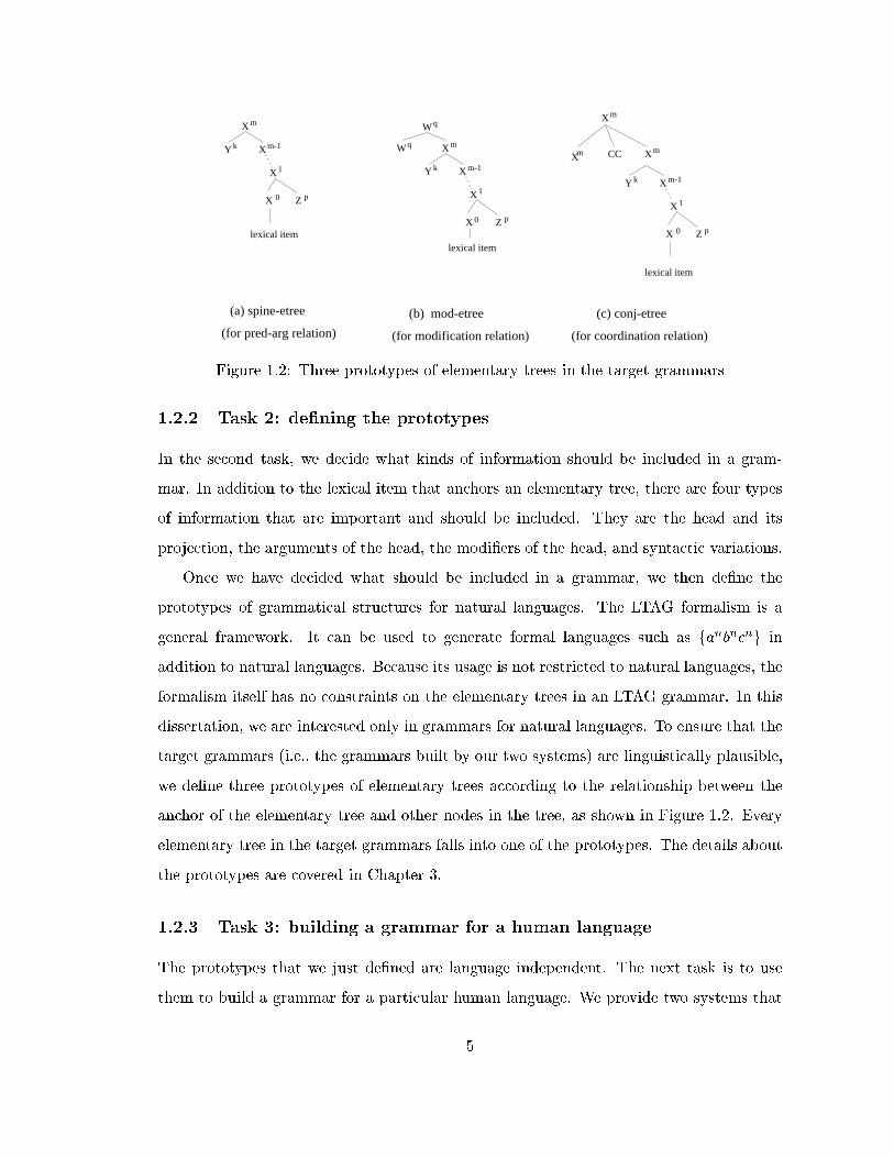
1.2.2 Task 2: de�ning the prototypes
In the second task, we decide what kinds of information should be included in a gram-
mar. In addition to the lexical item that anchors an elementary tree, there are four types
of information that are important and should be included. They are the head and its
projection, the arguments of the head, the modi�ers of the head, and syntactic variations.
Once we have decided what should be included in a grammar, we then de�ne the
prototypes of grammatical structures for natural languages. The LTAG formalism is a
general framework. It can be used to generate formal languages such as fanbncng in
addition to natural languages. Because its usage is not restricted to natural languages, the
formalism itself has no constraints on the elementary trees in an LTAG grammar. In this
dissertation, we are interested only in grammars for natural languages. To ensure that the
target grammars (i.e., the grammars built by our two systems) are linguistically plausible,
we de�ne three prototypes of elementary trees according to the relationship between the
anchor of the elementary tree and other nodes in the tree, as shown in Figure 1.2. Every
elementary tree in the target grammars falls into one of the prototypes. The details about
the prototypes are covered in Chapter 3.
1.2.3 Task 3: building a grammar for a human language
The prototypes that we just de�ned are language independent. The next task is to use
them to build a grammar for a particular human language. We provide two systems that
5
automatically generate grammars.
The �rst system, called LexOrg, generates elementary trees in a grammar by combining
tree descriptions. The main idea is as follows. Each elementary tree includes one or
more of the four types of information mentioned previously. They are the head and its
projections, the arguments of the head, the modi�ers of the head, and syntactic variations.
Each type of information by itself provides only a partial description of an elementary
tree, but combining these partial descriptions will provide complete information about
the elementary tree. LexOrg requires its users to specify tree descriptions for these four
types of information. To produce the grammar, LexOrg takes these tree descriptions as
the input and combines them to automatically generate the elementary trees. LexOrg
has two major advantages: �rst, grammars created by LexOrg are consistent because
elementary trees are generated automatically from tree descriptions; second, the underlying
linguistic information is expressed explicitly as tree descriptions, subcategorization frames,
and lexical rules. The details about LexOrg are covered in Chapter 4.
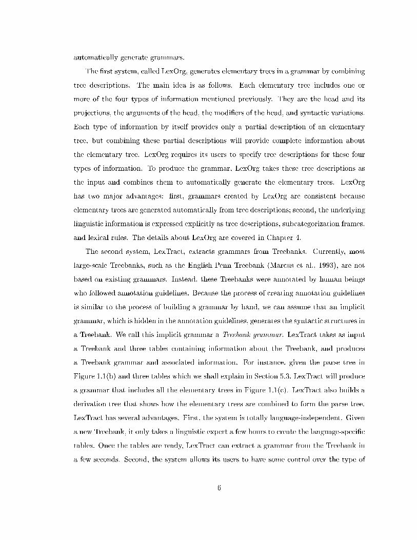
The second system, LexTract, extracts grammars from Treebanks. Currently, most
large-scale Treebanks, such as the English Penn Treebank (Marcus et al., 1993), are not
based on existing grammars. Instead, these Treebanks were annotated by human beings
who followed annotation guidelines. Because the process of creating annotation guidelines
is similar to the process of building a grammar by hand, we can assume that an implicit
grammar, which is hidden in the annotation guidelines, generates the syntactic structures in
a Treebank. We call this implicit grammar a Treebank grammar. LexTract takes as input
a Treebank and three tables containing information about the Treebank, and produces
a Treebank grammar and associated information. For instance, given the parse tree in
Figure 1.1(b) and three tables which we shall explain in Section 5.3, LexTract will produce
a grammar that includes all the elementary trees in Figure 1.1(c). LexTract also builds a
derivation tree that shows how the elementary trees are combined to form the parse tree.
LexTract has several advantages. First, the system is totally language-independent. Given
a new Treebank, it only takes a linguistic expert a few hours to create the language-speci�c
tables. Once the tables are ready, LexTract can extract a grammar from the Treebank in
a few seconds. Second, the system allows its users to have some control over the type of
6

traditional approach LexOrg LexTract
human e�ort tremendous (�) some (2) little (p)
exibility very little (�) some (2) some (2)
coverage hard to can be inferred covers the sourceevaluate (�) from the input (2) Treebank (2)
statistical info not available (�) not available (�) available (p)
consistency not guaranteed (�) consistent (p) not guaranteed (�)
generalization hidden in elementary expressed hidden in elementarytrees (�) explicitly (
p) trees (�)
Table 1.1: The comparison between three approaches for grammar development
Treebank grammar to be extracted. The users can run LexTract with di�erent settings to
get several di�erent Treebank grammars, and then choose the one that best �ts their goals.
Third, the system produces not only a Treebank grammar, but also the information about
how frequently certain elementary structures are combined to form syntactic structures.
This information can be used to train statistical parsers. In Chapters 5 and 6, we describe
LexTract and its applications in detail.
The di�erences between the traditional approach, LexOrg, and LexTract are summa-
rized in Table 1.1. We use the symbols �, 2, and p to indicate that an approach did not
solve the problem, partially solved the problem, and solved the problem, respectively. From
the table, it is clear that both LexOrg and LexTract have advantages over the traditional
approach.
1.3 Chapter summaries
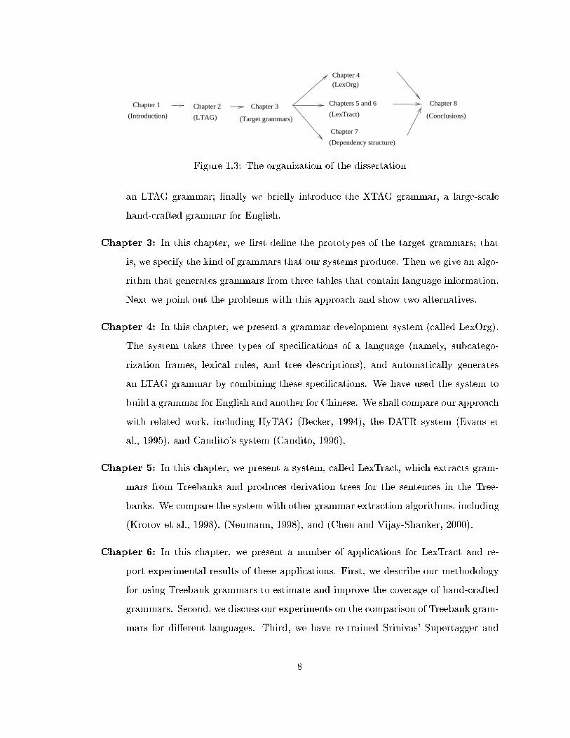
The structure of the dissertation is shown in Figure 1.3. An arrow from one chapter to an-
other indicates that the former should be read before the latter. Unlike many dissertations
that have a separate chapter for a literature survey, we include the comparison between
our approaches and related work in three individual chapters (i.e., Chapter 4, 5, and 7).
The following is a summary of the chapters in this dissertation:
Chapter 2: In this chapter, we �rst give a brief overview of the LTAG formalism; then
we discuss the properties of LTAG grammars; next we describe an extension of the
formalism (namely, multi-component TAGs); later we discuss the components of
7
(Introduction)
Chapter 1 Chapter 2
(LTAG)
Chapter 3
(Target grammars)
Chapter 7
(Dependency structure)
Chapters 5 and 6
(LexOrg)Chapter 4
Chapter 8
(Conclusions)(LexTract)
Figure 1.3: The organization of the dissertation
an LTAG grammar; �nally we brie y introduce the XTAG grammar, a large-scale
hand-crafted grammar for English.
Chapter 3: In this chapter, we �rst de�ne the prototypes of the target grammars; that
is, we specify the kind of grammars that our systems produce. Then we give an algo-
rithm that generates grammars from three tables that contain language information.
Next we point out the problems with this approach and show two alternatives.
Chapter 4: In this chapter, we present a grammar development system (called LexOrg).
The system takes three types of speci�cations of a language (namely, subcatego-
rization frames, lexical rules, and tree descriptions), and automatically generates
an LTAG grammar by combining these speci�cations. We have used the system to
build a grammar for English and another for Chinese. We shall compare our approach
with related work, including HyTAG (Becker, 1994), the DATR system (Evans et
al., 1995), and Candito's system (Candito, 1996).
Chapter 5: In this chapter, we present a system, called LexTract, which extracts gram-
mars from Treebanks and produces derivation trees for the sentences in the Tree-
banks. We compare the system with other grammar extraction algorithms, including
(Krotov et al., 1998), (Neumann, 1998), and (Chen and Vijay-Shanker, 2000).
Chapter 6: In this chapter, we present a number of applications for LexTract and re-
port experimental results of these applications. First, we describe our methodology
for using Treebank grammars to estimate and improve the coverage of hand-crafted
grammars. Second, we discuss our experiments on the comparison of Treebank gram-
mars for di�erent languages. Third, we have re-trained Srinivas' Supertagger and
8
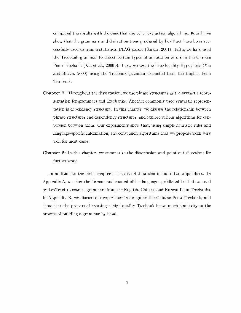
compared the results with the ones that use other extraction algorithms. Fourth, we
show that the grammars and derivation trees produced by LexTract have been suc-
cessfully used to train a statistical LTAG parser (Sarkar, 2001). Fifth, we have used
the Treebank grammar to detect certain types of annotation errors in the Chinese
Penn Treebank (Xia et al., 2000b). Last, we test the Tree-locality Hypothesis (Xia
and Bleam, 2000) using the Treebank grammar extracted from the English Penn
Treebank.
Chapter 7: Throughout the dissertation, we use phrase structures as the syntactic repre-
sentation for grammars and Treebanks. Another commonly used syntactic represen-
tation is dependency structure. In this chapter, we discuss the relationship between
phrase structures and dependency structures, and explore various algorithms for con-
version between them. Our experiments show that, using simple heuristic rules and
language-speci�c information, the conversion algorithms that we propose work very
well for most cases.
Chapter 8: In this chapter, we summarize the dissertation and point out directions for
further work.
In addition to the eight chapters, this dissertation also includes two appendices. In
Appendix A, we show the formats and content of the language-speci�c tables that are used
by LexTract to extract grammars from the English, Chinese and Korean Penn Treebanks.
In Appendix B, we discuss our experience in designing the Chinese Penn Treebank, and
show that the process of creating a high-quality Treebank bears much similarity to the
process of building a grammar by hand.
9

Chapter 2
Overview of LTAG
There are various grammar frameworks proposed for natural languages: Context-free gram-
mars (CFGs), Head Grammars (HGs), Head-driven Phrase Structure Grammars (HPSGs),
Combinatory Categorial Grammars (CCGs) and so on. For a discussion of the relations
among these formalisms, see (Weir, 1988; Kasper et al., 1995) among others. We take
Lexicalized Tree-adjoining Grammars (LTAGs) as representative of a class of lexicalized
grammars. LTAG is appealing for representing various phenomena in natural languages
due to its linguistic and computational properties. In the last decade, LTAG has been used
in several aspects of natural language understanding (e.g., parsing (Schabes, 1990; Srini-
vas, 1997), semantics (Joshi and Vijay-Shanker, 1999; Kallmeyer and Joshi, 1999), lexical
semantics (Palmer et al., 1999; Kipper et al., 2000), and discourse (Webber and Joshi,
1998; Webber et al., 1999)) and a number of NLP applications (e.g., machine translation
(Palmer et al., 1998), information retrieval (Chandrasekar and Srinivas, 1997), generation
(Stone and Doran, 1997; McCoy et al., 1992), and summarization applications (Baldwin
et al., 1997)).
LTAG is a formalism, rather than a grammar. To avoid the confusion, from now on,
we shall use the LTAG formalism to refer to the formalism, and use an LTAG grammar to
refer to a grammar that is based on the LTAG formalism.
In this chapter, we give an overview of the LTAG formalism and its relevance to natural
languages. Due to the large amount of work based on LTAG, the overview is not intended
to be comprehensive. Instead, we shall focus on the aspects that are most relevant to this
10

dissertation. For a more comprehensive discussion on the formalism, see (Joshi et al., 1975;
Joshi, 1985; Joshi, 1987; Joshi and Schabes, 1997). This chapter is organized as follows.
In Section 2.1, we give a brief introduction of the basic LTAG formalism. In Section
2.2, we discuss the properties of LTAG that make it an appealing formalism for natural
language processing. In Section 2.3, we describe an extension of the LTAG formalism,
namely, Multi-component TAG (MCTAG). In Section 2.4, we introduce the components
of an LTAG grammar. In Section 2.5, we brie y discuss the XTAG English grammar,
which is going to be used in later chapters.
2.1 Basics of the LTAG formalism
LTAGs are based on the Tree Adjoining Grammar (TAG) formalism developed by Joshi,
Levy, and Takahashi (Joshi et al., 1975; Joshi and Schabes, 1997).
2.1.1 Elementary trees
The primitive elements of an LTAG are elementary trees. An LTAG is lexicalized, as each
elementary tree is associated with at least one lexical item (which is called the anchor of
the tree) on its frontier. The elementary trees are minimal in the sense that all and only
the arguments of the anchor are encapsulated in the tree. The elementary trees of LTAG
possess an extended domain of locality. The grammatical constraints are stated over the
elementary trees, and are independent of all recursive processes. There are two types of
elementary trees: initial trees and auxiliary trees. Each auxiliary tree has a unique leaf
node, called the foot node, which has the same label as the root. In both types of trees,
leaf nodes other than anchors and foot nodes are called substitution nodes.
2.1.2 Two operations
Elementary trees are combined by two operations: substitution and adjoining. In the sub-
stitution operation (see Figure 2.1), a substitution node in an elementary tree is replaced
by another elementary tree whose root has the same label as the substitution node. In an
adjoining operation (see Figure 2.2), an auxiliary tree is inserted into another elementary
11

=>
X
Y
Y X
Y
Figure 2.1: The substitution operation
=>Y
Y
X
Y
X
Y
Y
Figure 2.2: The adjoining operation
tree. The root and the foot nodes of the auxiliary tree must match the node label at which
the auxiliary tree adjoins. The resulting structure of the combined elementary trees is
called a parse tree or a derived tree. The history of the combination process is recorded as
a derivation tree.
In Figure 2.3, the four elementary trees in (a) are anchored by words in the sentence
underwriters still draft policies. �1 | �3 are initial trees, and �1 is an auxiliary tree. Foot
and substitution nodes are marked by � and #, respectively. To generate the derived tree
for the sentence, �1 and �3 substitute into the nodes NP0 and NP1 in �2 respectively, and
�1 adjoins to the VP node in �2, thus forming the derived tree in (b). The solid and dash
arrows between the elementary trees stand for the substitution and adjoining operations,
respectively. The history of the composition of the elementary trees is recorded in the
derivation tree in (c). In a derivation tree, a dash line is used for an adjoining operation
and a solid line for substitution. The number within square brackets is the address of the
node at which the substitution/adjoining operation took place. The address is useful when
there are two or more nodes with the same label in an elementary tree. For the sake of
simplicity, from now on we shall drop these addresses from derivation trees.
12

(underwriters)α1β1(still)
α3(policies)
α2 (draft)
[2.2][2]
[1]
(a) elementary trees
0
1
underwriters
ADVP VP*
still
VP
NP
S
VP
NP
draft
NP
policies
NP
NNADV V
(b) derived tree
underwriters
NP VP
ADVP VP
still draft
NP
S
policies
N
ADV V
N
α1:αα2: 3:β1:
(c) derivation tree
Figure 2.3: Elementary trees, derived tree and derivation tree for underwriters still draftpolicies.
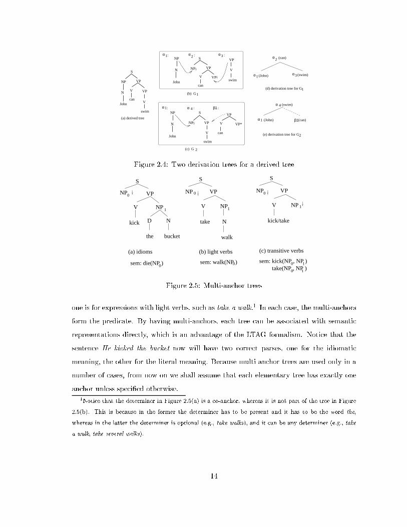
2.1.3 Derived trees and derivation trees
Unlike in CFGs, the derived trees and derivation trees in the LTAG formalism are not
identical; that is, several derivation trees may produce the same derived tree. For instance,
in Figure 2.4, G1 in (b) and G2 in (c) are two di�erent grammars. The derived tree in (a)
can be produced by combining either the elementary trees in G1 or the ones in G2. The
corresponding derivation trees are shown in (d) and (e). This property becomes relevant in
Chapter 5, where we discuss a system, LexTract, that automatically constructs elementary
trees and derivation trees from derived trees.
2.1.4 Multi-anchor trees
An elementary tree is normally anchored by a single lexical item, but multi-anchor trees
are used in a number of cases. Two of them are shown in Figure 2.5(a) and 2.5(b). The
�rst one is for idioms such as kick the bucket (which means someone dies), and the second
13
α3 (swim)α1 (John)
α2 (can)
(d) derivation tree for G1
α 4
α1 (John) β1(can)
(swim)
(e) derivation tree for G2
S
VP
VPV
canV
swim
John
NP
N
(a) derived tree
NP
N
John
α2 α3α1
NP
N
John
β1α 4α1
S
VPNP
V
can
VP
VP
V
swim
: : :
(b) G1
(c) G 2
S
V
swim
VP
can
NP VP V
: : :
VP*
Figure 2.4: Two derivation trees for a derived tree
take(NP , NP )0 1
10sem: kick(NP , NP )0sem: walk(NP )0sem: die(NP )
1
0
1
0
1
0NP VP
V NP
kick/take
S
VPNP
NP
Ntake
walk
S
V
(a) idioms (c) transitive verbs(b) light verbs
bucketthe
kick ND
NPV
VPNP
S
Figure 2.5: Multi-anchor trees
one is for expressions with light verbs, such as take a walk.1 In each case, the multi-anchors
form the predicate. By having multi-anchors, each tree can be associated with semantic
representations directly, which is an advantage of the LTAG formalism. Notice that the
sentence He kicked the bucket now will have two correct parses, one for the idiomatic
meaning, the other for the literal meaning. Because multi-anchor trees are used only in a
number of cases, from now on we shall assume that each elementary tree has exactly one
anchor unless speci�ed otherwise.
1Notice that the determiner in Figure 2.5(a) is a co-anchor, whereas it is not part of the tree in Figure
2.5(b). This is because in the former the determiner has to be present and it has to be the word the,
whereas in the latter the determiner is optional (e.g., take walks), and it can be any determiner (e.g., take
a walk, take several walks).
14
tr
brY
t U tr
X
Ybr
t
=>
X
Y
Figure 2.6: The substitution operation with features
>
X
tYb
Y
Y*
br
tf
bf
trX
t U tr
b U bf
tf
br
Y
Y
Figure 2.7: The adjoining operation with features
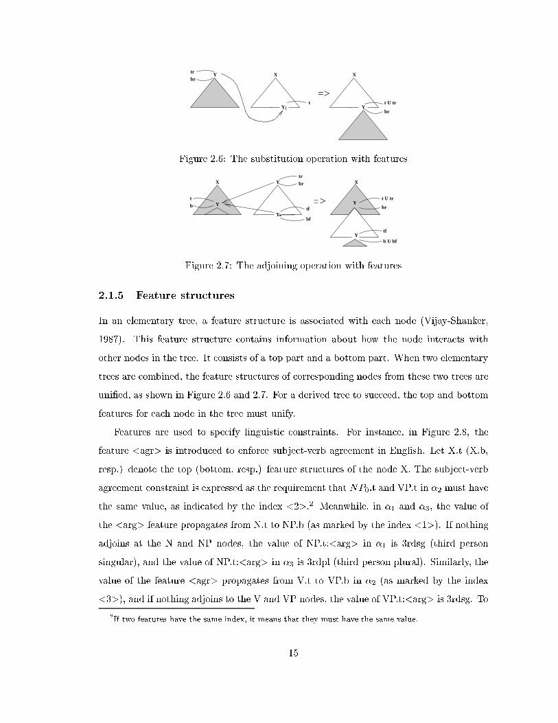
2.1.5 Feature structures
In an elementary tree, a feature structure is associated with each node (Vijay-Shanker,
1987). This feature structure contains information about how the node interacts with
other nodes in the tree. It consists of a top part and a bottom part. When two elementary
trees are combined, the feature structures of corresponding nodes from these two trees are
uni�ed, as shown in Figure 2.6 and 2.7. For a derived tree to succeed, the top and bottom
features for each node in the tree must unify.
Features are used to specify linguistic constraints. For instance, in Figure 2.8, the
feature <agr> is introduced to enforce subject-verb agreement in English. Let X.t (X.b,
resp.) denote the top (bottom, resp.) feature structures of the node X. The subject-verb
agreement constraint is expressed as the requirement that NP0.t and VP.t in �2 must have
the same value, as indicated by the index <2>.2 Meanwhile, in �1 and �3, the value of
the <arg> feature propagates from N.t to NP.b (as marked by the index <1>). If nothing
adjoins at the N and NP nodes, the value of NP.t:<arg> in �1 is 3rdsg (third person
singular), and the value of NP.t:<arg> in �3 is 3rdpl (third person plural). Similarly, the
value of the feature <agr> propagates from V.t to VP.b in �2 (as marked by the index
<3>), and if nothing adjoins to the V and VP nodes, the value of VP.t:<arg> is 3rdsg. To
2If two features have the same index, it means that they must have the same value.
15

John
N
NP
[agr: <1>]
[agr:<1>][]
[agr: 3rdsg]
VP
α1:
NP0 [][arg:<2>]
V
likes
[agr:3rdsg][agr:<3>]
[agr:<3>][agr:<2>]
NP1
Sα2: α3:
N
NP
[agr: <1>]
[agr:<1>][]
dogs
[agr: 3rdpl]
Figure 2.8: Features for the subject-verb agreement
S
a S d
S
b S cNA
NA
ε
Figure 2.9: An LTAG grammar that generates the language fanbncndng
parse the sentence John likes dogs, �1 substitutes into the NP0 node in �2, and the values
of NP0.t:<agr> and VP.t:<agr> agree. For the sentence Dogs likes John, �3 substitutes
into the NP0 node, but the values of NP0.t:<agr> and VP.t:<agr> are di�erent and
cannot unify; therefore, the subject-verb agreement constraint is violated. This example
shows that, with the subject-verb agreement constraint, the toy grammar that consists
of only three elementary trees in Figure 2.8 can correctly accept the former sentence and
reject the latter.
From now on, for the sake of simplicity, we shall not show the feature structures in
elementary trees unless necessary.
2.2 LTAG for natural languages
LTAG is a constrained mathematical formalism. As a formalism, LTAG is more powerful
than CFG in that an LTAG grammar can generate a mildly context-sensitive language.
For example, the grammar in Figure 2.9 generates the language fanbncndng, which is a
content-sensitive language. The NAs in the �rst elementary tree mark that no adjoining
operations are allowed at the S nodes.
16

LTAG is an appealing formalism for representing various phenomena, especially syntac-
tic phenomena, in natural languages because of its linguistic and computational properties,
some of which are listed below:
� Lexicalized grammar: A grammar in the LTAG formalism is fully lexicalized in the
sense that each elementary tree is associated with a lexical item. It is generally
agreed that lexicalized grammars are preferred over non-lexicalized grammars for
NLP tasks such as parsing (Schabes, 1990).
� Extended Domain of Locality: Every elementary tree encapsulates all and only the
arguments of the anchor; thus, elementary trees provide extended locality over which
the syntactic and semantic constraints can be speci�ed. This is in contrast with
CFGs, where the arguments of the predicate may appear in separate context-free
rules. For example, the subject and the object of a transitive verb appear in two
rules: (1) S ! subject VP, and (2) VP ! V object.
� Generative capacity: Recent research (Bresnan et al., 1982; Higginbotham, 1984;
Shieber, 1984) has found that natural languages are beyond context free. For in-
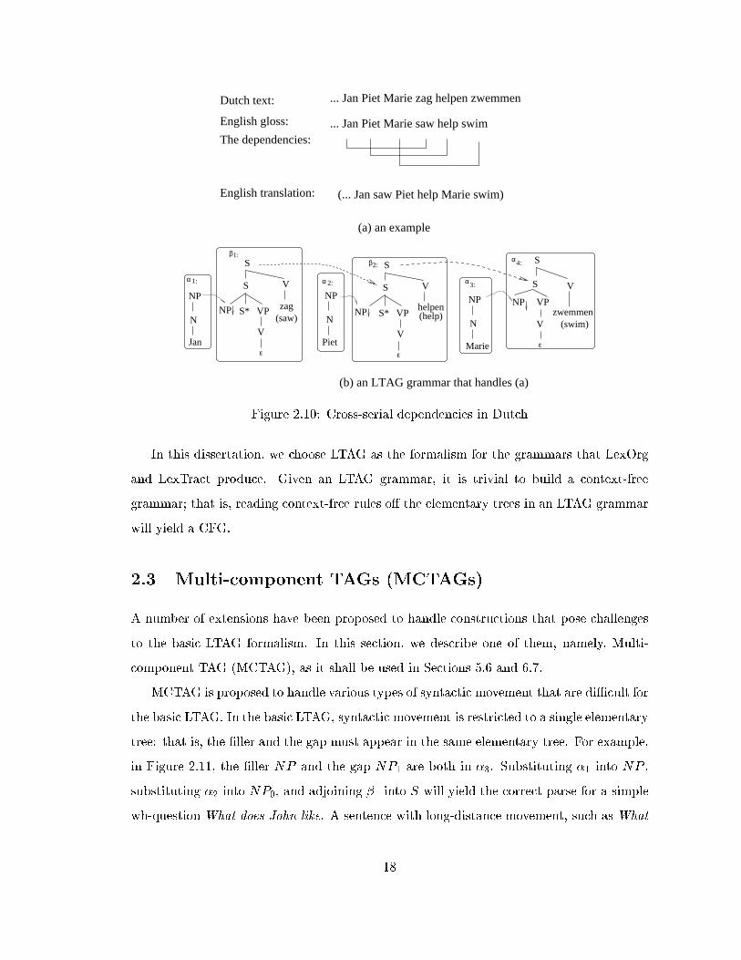
stance, the cross-serial dependency relation in Dutch is context-sensitive. In this
aspect, LTAG is appealing because it is more powerful than CFG, but only \mildly"
so (Joshi et al., 1975; Joshi, 1985; Joshi, 1987). As shown in (Joshi, 1985), LTAG, but
not CFG, can handle cross-serial dependencies in Dutch. An example of cross-serial
dependencies and its treatment in LTAG are shown in Figure 2.10.3
On the other hand, the parsing time for an LTAG grammar is O(n6), where n is the
sentence length; that is, given an LTAG grammar, an LTAG parser can produce a tree
forest that includes all possible parse trees for a sentence of length n in O(n6). This is
much longer than the parsing time for a CFG grammar, which is O(n3). To address the
eÆciency issue, people have proposed some variances of the LTAG formalism. One of them
is the Tree Insertion Grammar (Schabes and Waters, 1995), which is weakly equivalent to
CFG and has O(n3) parsing time.
3Both the example and the grammar in Figure 2.10 come from (Joshi, 1985). We changed the grammar
slightly to be consistent with current notation conventions.
17
S
S V
helpenVPS* (help)NP
V
ε
β1:
NP
N
Jan
N
NP
Piet
NP
N
Marie
2:β
α 1: α3:
α4:
α 2: V
NP VP
V
ε
(swim)zwemmen
S
S
VP
VS
S
S*
V
ε
zag(saw)
NP
(... Jan saw Piet help Marie swim)
... Jan Piet Marie saw help swim
Dutch text:
English gloss:
The dependencies:
English translation:
(a) an example
... Jan Piet Marie zag helpen zwemmen
(b) an LTAG grammar that handles (a)
Figure 2.10: Cross-serial dependencies in Dutch
In this dissertation, we choose LTAG as the formalism for the grammars that LexOrg
and LexTract produce. Given an LTAG grammar, it is trivial to build a context-free
grammar; that is, reading context-free rules o� the elementary trees in an LTAG grammar
will yield a CFG.
2.3 Multi-component TAGs (MCTAGs)
A number of extensions have been proposed to handle constructions that pose challenges
to the basic LTAG formalism. In this section, we describe one of them, namely, Multi-
component TAG (MCTAG), as it shall be used in Sections 5.6 and 6.7.
MCTAG is proposed to handle various types of syntactic movement that are diÆcult for
the basic LTAG. In the basic LTAG, syntactic movement is restricted to a single elementary
tree: that is, the �ller and the gap must appear in the same elementary tree. For example,
in Figure 2.11, the �ller NP and the gap NP1 are both in �3. Substituting �1 into NP ,
substituting �2 into NP0, and adjoining �1 into S will yield the correct parse for a simple
wh-question What does John like. A sentence with long-distance movement, such as What
18

S
S*V
does
NP
N
John
NP
N
what
α2:
α1: α 3:β1:
(a) elementary trees (b) derived tree
S
NP S
NP VP
V NP
εlike
0
1
NP VP
V NP
εlike
0
1N
John
S
SNP
N
what
V
does
S
Figure 2.11: Trees for the wh-question What does John like
S
S*V
does
think
S
NP VP
V S*
S
NP VP
V S*
S
NP S
NP VP
V NP
εlikes
0
1
believes
2:β β3:α1: β1:
(b) derived tree(a) elementary trees
S
V
think
NP VP
NP
NP
S
V S
NP
N
VP
S
VPNP
S
John
N
V
N
ε
Mary
Mike believes
doesN
what
V
likes
Figure 2.12: Trees for the wh-question What does Mary think Mike believes John likes
does Mary think Mike believes John likes, is handled similarly, as shown in Figure 2.12.
This type of movement is \unbounded" in the sense that in the sentence there can be an
unbounded number of verbs between the �ller and the gap, but the treatment in the LTAG
formalism is still elementary tree bound in the sense that the gap and the �ller are in the
same elementary tree.
This analysis runs into problems when the moved constituent is an adjunct. In Figure
2.13(a), the NP trace and the �ller NP cannot be in the same elementary tree because
the PP (the parent of the NP trace) is a modi�er of the VP and therefore should not be
part of the elementary tree anchored by the verb stay. An MCTAG is required to handle
such cases. MCTAG extends the basic LTAG so that the adjoining operation in MCTAG
is de�ned on elementary tree sets rather than on a single elementary tree. Weir (1988)
gave four ways of de�ning the adjoining operation. Two of them are commonly used in
the literature. One is called tree-local MCTAG, which requires the elementary trees in a
19
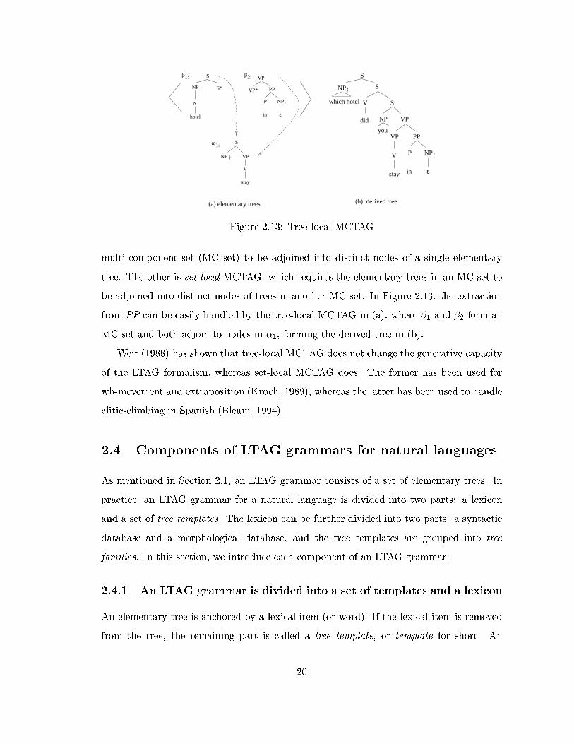
NP
N
hotel
S*
S
NP VP
V
stay
S
VP
PP
NP
ε
VP*
P
in
i
i
α 1:
β1: β2:
NP
which hotel
iS
V
did
S
NP
you
VP
VP
V
stay
PP
P NP
in ε
i
S
(a) elementary trees (b) derived tree
Figure 2.13: Tree-local MCTAG
multi-component set (MC set) to be adjoined into distinct nodes of a single elementary
tree. The other is set-local MCTAG, which requires the elementary trees in an MC set to
be adjoined into distinct nodes of trees in another MC set. In Figure 2.13, the extraction
from PP can be easily handled by the tree-local MCTAG in (a), where �1 and �2 form an
MC set and both adjoin to nodes in �1, forming the derived tree in (b).
Weir (1988) has shown that tree-local MCTAG does not change the generative capacity
of the LTAG formalism, whereas set-local MCTAG does. The former has been used for
wh-movement and extraposition (Kroch, 1989), whereas the latter has been used to handle
clitic-climbing in Spanish (Bleam, 1994).
2.4 Components of LTAG grammars for natural languages
As mentioned in Section 2.1, an LTAG grammar consists of a set of elementary trees. In
practice, an LTAG grammar for a natural language is divided into two parts: a lexicon
and a set of tree templates. The lexicon can be further divided into two parts: a syntactic
database and a morphological database, and the tree templates are grouped into tree
families. In this section, we introduce each component of an LTAG grammar.
2.4.1 An LTAG grammar is divided into a set of templates and a lexicon
An elementary tree is anchored by a lexical item (or word). If the lexical item is removed
from the tree, the remaining part is called a tree template, or template for short. An
20
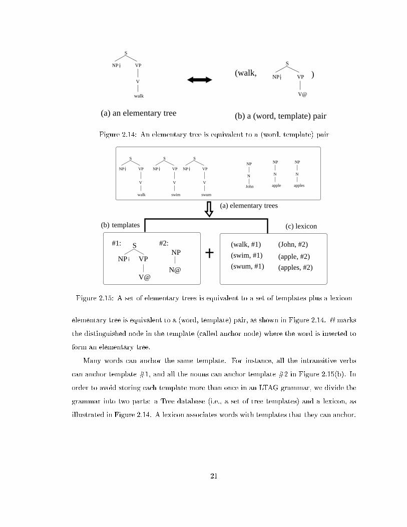
S
V
walk
NP VP S
V@
NP VP(walk, )
(a) an elementary tree (b) a (word, template) pair
Figure 2.14: An elementary tree is equivalent to a (word, template) pair
S
V
walk
NP VP
S
V
NP VP
swim
S
V
NP VPNP
John
N
NP
N
apple
NP
N
apples
(walk, #1)
(swim, #1)
(swum, #1)
(John, #2)
(apple, #2)
(apples, #2)
templates(b)
(a) elementary trees
#1: #2:NP
N@V@
VPNP
S
swum
(c) lexicon
Figure 2.15: A set of elementary trees is equivalent to a set of templates plus a lexicon
elementary tree is equivalent to a (word, template) pair, as shown in Figure 2.14. @ marks
the distinguished node in the template (called anchor node) where the word is inserted to
form an elementary tree.
Many words can anchor the same template. For instance, all the intransitive verbs
can anchor template #1, and all the nouns can anchor template #2 in Figure 2.15(b). In
order to avoid storing each template more than once in an LTAG grammar, we divide the
grammar into two parts: a Tree database (i.e., a set of tree templates) and a lexicon, as
illustrated in Figure 2.14. A lexicon associates words with templates that they can anchor.
21
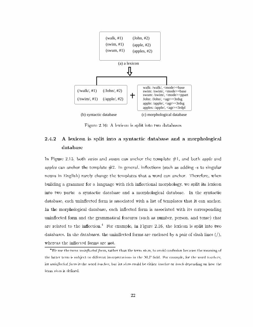
(walk, #1)
(swim, #1)
(swum, #1)
(John, #2)
(apple, #2)
(apples, #2)
walk: /walk/, <mode>=baseswim: /swim/, <mode>=baseswum: /swim/, <mode>=ppartJohn: /John/, <agr>=3rdsgapple: /apple/, <agr>=3rdsgapples: /apple/, <agr>=3rdpl
(/John/, #2)
(/apple/, #2)
(/walk/, #1)
(/swim/, #1)
(a) a lexicon
(c) morphological database(b) syntactic database
Figure 2.16: A lexicon is split into two databases
2.4.2 A lexicon is split into a syntactic database and a morphological
database
In Figure 2.15, both swim and swam can anchor the template #1, and both apple and
apples can anchor the template #2. In general, in ections (such as adding -s to singular
nouns in English) rarely change the templates that a word can anchor. Therefore, when
building a grammar for a language with rich in ectional morphology, we split its lexicon
into two parts: a syntactic database and a morphological database. In the syntactic
database, each unin ected form is associated with a list of templates that it can anchor.
In the morphological database, each in ected form is associated with its corresponding
unin ected form and the grammatical features (such as number, person, and tense) that
are related to the in ection.4 For example, in Figure 2.16, the lexicon is split into two
databases. In the databases, the unin ected forms are enclosed by a pair of slash lines (/),
whereas the in ected forms are not.
4We use the term unin ected form, rather than the term stem, to avoid confusion because the meaning of
the latter term is subject to di�erent interpretations in the NLP �eld. For example, for the word teachers,
its unin ected form is the word teacher, but its stem could be either teacher or teach depending on how the
term stem is de�ned.
22
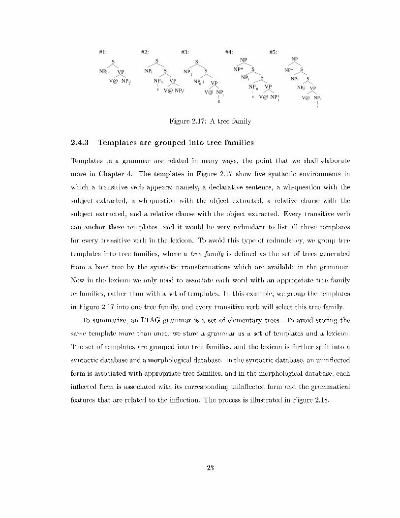
0
1
VPNP
S
V@ NP
NP
ε
NP 0
S
VP
V@ NP1
S
ε
0
1V@
NP
NP
VP
SNP
S
NP*
S
NP
S
NP
ε
NP 0
V@
VP
1NP
0
NP
NP* S
NP S
NP VP
V@ NP1
ε
#3: #4: #5:#2:#1:
Figure 2.17: A tree family
2.4.3 Templates are grouped into tree families
Templates in a grammar are related in many ways, the point that we shall elaborate
more in Chapter 4. The templates in Figure 2.17 show �ve syntactic environments in
which a transitive verb appears; namely, a declarative sentence, a wh-question with the
subject extracted, a wh-question with the object extracted, a relative clause with the
subject extracted, and a relative clause with the object extracted. Every transitive verb
can anchor these templates, and it would be very redundant to list all these templates
for every transitive verb in the lexicon. To avoid this type of redundancy, we group tree
templates into tree families, where a tree family is de�ned as the set of trees generated
from a base tree by the syntactic transformations which are available in the grammar.
Now in the lexicon we only need to associate each word with an appropriate tree family
or families, rather than with a set of templates. In this example, we group the templates
in Figure 2.17 into one tree family, and every transitive verb will select this tree family.
To summarize, an LTAG grammar is a set of elementary trees. To avoid storing the
same template more than once, we store a grammar as a set of templates and a lexicon.
The set of templates are grouped into tree families, and the lexicon is further split into a
syntactic database and a morphological database. In the syntactic database, an unin ected
form is associated with appropriate tree families, and in the morphological database, each
in ected form is associated with its corresponding unin ected form and the grammatical
features that are related to the in ection. The process is illustrated in Figure 2.18.
23

S
V
NP VP S
NP VP
V
S
NP
S
NP S
NP VP
V NP
S
NP VP
V NP
S
NP VP
S
NP
V@
S
NP VP
NPV@
templates(b) (c) lexicon
(a) elementary trees
buysswumswum buys
(/swim/, Tnx0V)
(/buy/, Tnx0Vnx1)
(/walk/, Tnx0V)
(/die/, Tnx0V)......
......
swum: /swim/, <mode>=ppart
buys: /buy/, <mode>=present
<agr> = 3rdsing
walk: /walk/, <mode>=base
died: /die/, <mode>=ppart/past......
morphological databasesyntactic database
......
S
NP S
NP VP
NP
NP
S
VP
V@
V@
Tnx0Vnx1:
Tnx0V:
Figure 2.18: The components of an LTAG grammar
2.5 The XTAG grammar
There have been a number of LTAG grammars developed at the University of Pennsylvania
and elsewhere in the world for languages such as English, French, Chinese, and Korean.
Among them, arguably the most well-known one is the XTAG English grammar, which is
a large-scale English grammar that has been developed by the XTAG Research Group at
the University of Pennsylvania since the early 1990s.5 The latest version of the grammar
was released to the public in March 2001. It has 1226 templates. The templates for verbs
are grouped into 57 tree families. The morphological database has entries for about 317
thousand in ected words, and the syntactic database has entries for about 30 thousand
unin ected words. Conceptually, there are 1.8 million elementary trees in total. The
templates of the grammar were built by hand, whereas the lexicon was extracted from two
dictionaries (Oxford Dictionary for Contemporary Idiomatic English and Oxford Advanced
Learner's Dictionary) and then manually checked. For more information about the XTAG
5XTAG is the name of a system that allows grammar developers to build and test LTAG grammars
in the X-window environment. The name is also used to refer to the research group at the University of
Pennsylvania who has built and used the system for language processing.
24
grammar, please refer to (Group, 2001).
In Sections 4.8 and 6.2, we compare the grammars built by LexOrg and LexTract with
an early version of the XTAG grammar, which has 1004 tree templates. The templates
for verbs are grouped into 53 tree families. Some common families are intransitive (e.g.,
sleep), transitive (e.g., buy), ditransitive (e.g., ask), ergative (e.g., melt), intransitive verb
particle (e.g., sign o�), transitive verb particle (e.g., pick up), and so on.
2.6 Summary
To summarize this chapter, LTAG is a tree rewriting system. An LTAG consists of a set of
elementary trees, which are combined via two operations (substitution and adjoining) to
form a parse tree (derived tree) for a sentence. LTAG is appealing for the representation of
various phenomena in natural languages due to its linguistic and computational properties.
To handle various phenomena in natural language, a number of extensions of the basic
LTAG have been proposed. MCTAG is one of them, and it is aimed at handling various
types of syntactic movement. In practice, an LTAG grammar is divided into a lexicon
and a set of templates. The lexicon can be further divided into two parts: a syntactic
database and a morphological database, and the tree templates are grouped into tree
families. Finally, we brie y discuss the XTAG English grammar, which is going to be used
in later chapters.
25
Chapter 3
The target grammars
In Chapter 2, we gave a brief introduction to the LTAG formalism and its main properties.
In the next two chapters, we describe two systems that we designed to facilitate gram-
mar development: LexOrg generates grammars from descriptions, and LexTract extracts
grammars from Treebanks. Before getting into the detail of the systems, we would like to
�rst de�ne the prototypes of the target grammars; that is, we specify the kind of gram-
mars that our systems produce. Then we give an algorithm that generates grammars from
language-speci�c tables. Next we point out the problems with this approach and show the
two alternatives that address these problems.
3.1 Four types of structural information
In this chapter, we �rst de�ne the kind of LTAG grammars that our systems build for
natural languages. Recall that the LTAG formalism is a general framework. It can be used
to generate formal languages such as fanbncng in addition to natural languages. Because
its usage is not restricted to natural languages, the formalism itself has no constraints on
the elementary trees in an LTAG grammar other than the basic requirements that each
elementary tree must be anchored by a lexical item and an auxiliary tree should have
exactly one foot node which has the same category as the root node. In this dissertation,
we are interested only in grammars for natural languages. To ensure that the target
grammars (i.e., the grammars built by LexOrg or LexTract) are linguistically plausible,
26

we de�ne three prototypes such that every elementary tree in the target grammars should
fall into one of the prototypes.1
Before we de�ne prototypes of elementary trees, let us �rst determine what kind of
information should be included in elementary trees. In addition to the lexical item that
anchors an elementary tree, there are four types of information that are important and
should be included. In this section, we look at each type in detail and discuss how it
is represented in LTAG grammars and linguistic theories such as X-bar theory and GB
theory.
3.1.1 Head and its projections
An important notion in many contemporary linguistic theories such as X-bar theory and
GB theory is the notion of head. A head determines the main properties of the phrase that
it belongs to. A head may project to various levels, and the head and its projections form
a projection chain. For instance, in X-bar theory (see Figure 3.1(a)), a head X projects to
�X, and the �X projects to XP . The X in this paradigm can be any part of speech such as
a verb, where the XP is a phrase such as a verb phrase. GB theory divides heads into two
types: lexical heads and functional heads. In Figure 3.1(b), V (for verb) is a lexical head,
whereas C (for complementizer) and I (for in ection) are functional heads. The projections
of lexical and functional heads are called lexical and functional projections, respectively.
An LTAG grammar does not have to strictly follow a linguistic theory. In practice,
to make the elementary trees simple and theory neutral, LTAG grammar developers often
choose to omit certain projections, to treat function projections and lexical projections dif-
ferently, and not to represent certain internal movements. Figure 3.2 shows four templates
in the XTAG grammar. Among them, template #2 can be seen as a simpli�ed version of
the structure in Figure 3.1(b): the template does not have the �V , �I, and �C levels; it uses
the same label S for IP and CP nodes; it does not include the complementizer C and the
INFL nodes; it does not show the movement of the subject from the [Spec, VP] position
to the [Spec, IP] position.
1Another possible name for a prototype is template. We do not use this name because the term template
in the LTAG formalism is used to refer to an unlexicalized elementary tree.
27
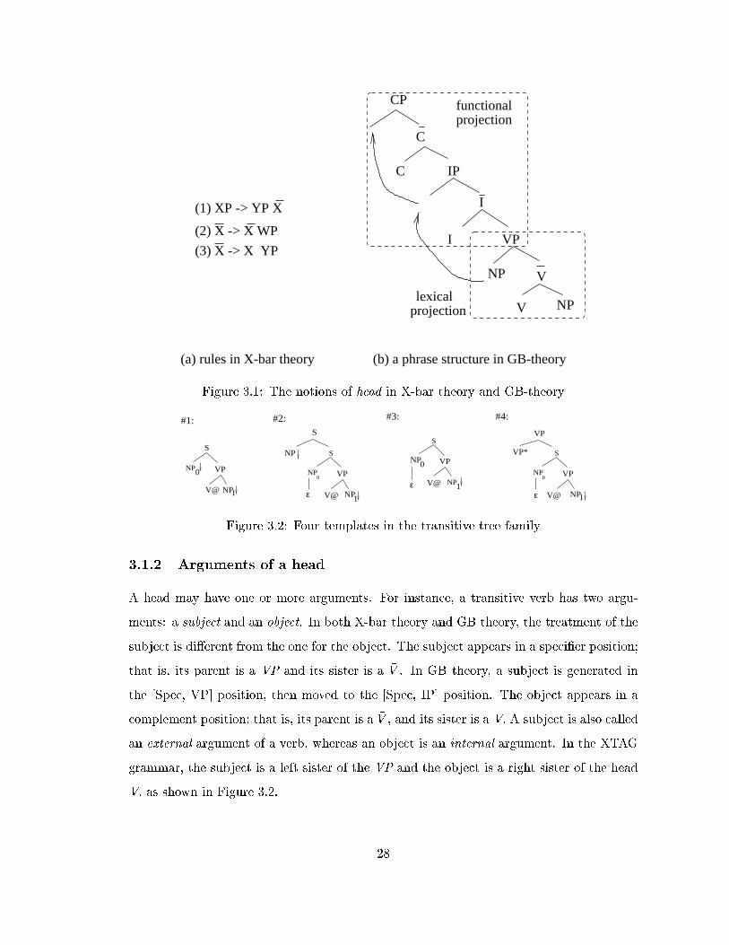
projectionlexical
functionalprojection
CP
C
C IP
I
I
VP
V
NPV
NP
(1) XP -> YP X
(3) X -> X YP
(2) X -> X WP
(a) rules in X-bar theory (b) a phrase structure in GB-theory
Figure 3.1: The notions of head in X-bar theory and GB-theory
S
NPV@
VPNP 0
1ε
#1: #4:
S
0NP
#2:
S
NP 0
#3:
VP*
V@ NP
VP
NPV@
VPNP VP
V@ NP1
NP
S
1 1
0
VP
S
ε ε
Figure 3.2: Four templates in the transitive tree family
3.1.2 Arguments of a head
A head may have one or more arguments. For instance, a transitive verb has two argu-
ments: a subject and an object. In both X-bar theory and GB theory, the treatment of the
subject is di�erent from the one for the object. The subject appears in a speci�er position;
that is, its parent is a VP and its sister is a �V . In GB theory, a subject is generated in
the [Spec, VP] position, then moved to the [Spec, IP] position. The object appears in a
complement position; that is, its parent is a �V , and its sister is a V. A subject is also called
an external argument of a verb, whereas an object is an internal argument. In the XTAG
grammar, the subject is a left sister of the VP and the object is a right sister of the head
V, as shown in Figure 3.2.
28
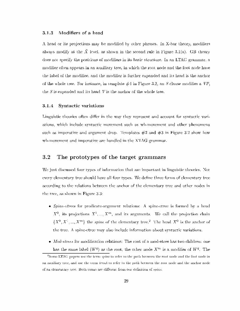
3.1.3 Modi�ers of a head
A head or its projections may be modi�ed by other phrases. In X-bar theory, modi�ers
always modify at the �X level, as shown in the second rule in Figure 3.1(a). GB theory
does not specify the positions of modi�ers in its basic structure. In an LTAG grammar, a
modi�er often appears in an auxiliary tree, in which the root node and the foot node have
the label of the modi�ee, and the modi�er is further expanded and its head is the anchor
of the whole tree. For instance, in template #4 in Figure 3.2, an S clause modi�es a VP,
the S is expanded and its head V is the anchor of the whole tree.
3.1.4 Syntactic variations
Linguistic theories often di�er in the way they represent and account for syntactic vari-
ations, which include syntactic movement such as wh-movement and other phenomena
such as imperative and argument drop. Templates #2 and #3 in Figure 3.2 show how
wh-movement and imperative are handled in the XTAG grammar.
3.2 The prototypes of the target grammars
We just discussed four types of information that are important in linguistic theories. Not
every elementary tree should have all four types. We de�ne three forms of elementary tree
according to the relations between the anchor of the elementary tree and other nodes in
the tree, as shown in Figure 3.3:
� Spine-etrees for predicate-argument relations: A spine-etree is formed by a head
X0, its projections X1; :::;Xm, and its arguments. We call the projection chain
fX0;X1; :::;Xmg the spine of the elementary tree.2 The head X0 is the anchor of
the tree. A spine-etree may also include information about syntactic variations.
� Mod-etrees for modi�cation relations: The root of a mod-etree has two children: one
has the same label (W q) as the root, the other node Xm is a modi�er of W q. The2Some LTAG papers use the term spine to refer to the path between the root node and the foot node in
an auxiliary tree, and use the term trunk to refer to the path between the root node and the anchor node
of an elementary tree. Both terms are di�erent from our de�nition of spine.
29
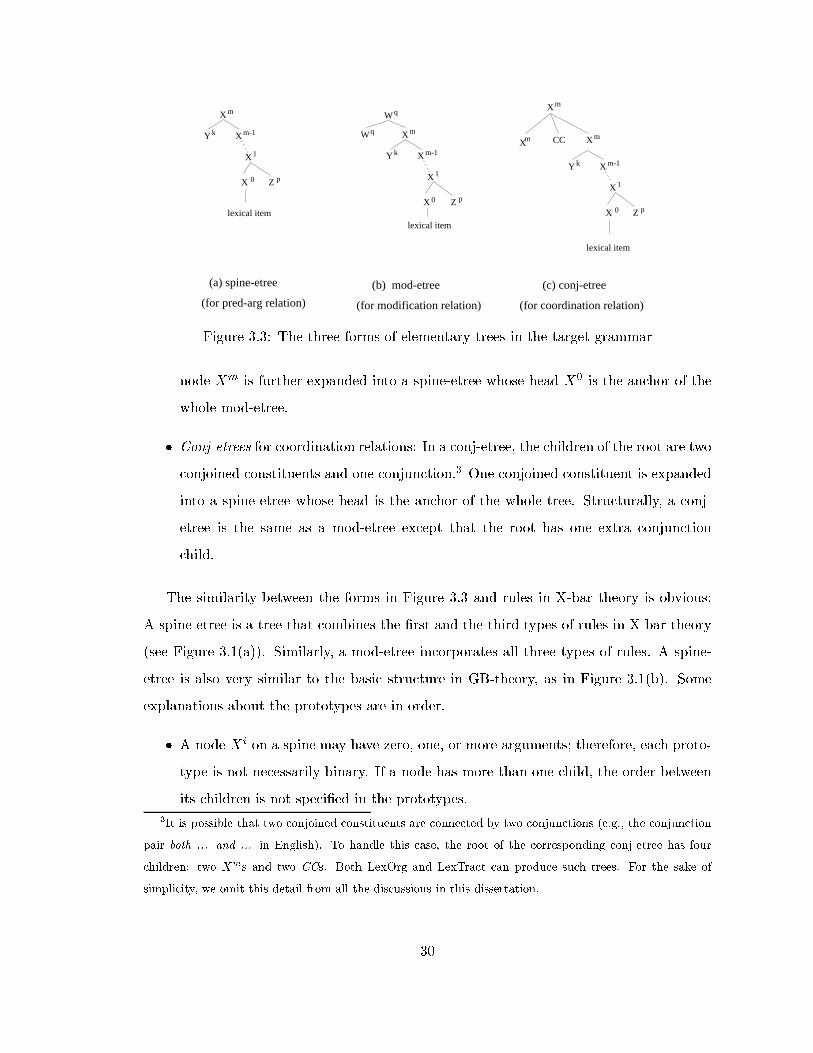
lexical item
CC
X
X
m
mXm
Y X
X
X Z
m-1
1
p
k
0
X
X
X Z
W
W
X
Y
lexical item
m-1
1
p
q
q
m
k
0
X
X
X Z
lexical item
X
Y m-1
1
p
m
k
0
(for coordination relation)
(c) conj-etree
(for modification relation)
(b) mod-etree
(for pred-arg relation)
(a) spine-etree
Figure 3.3: The three forms of elementary trees in the target grammar
node Xm is further expanded into a spine-etree whose head X0 is the anchor of the
whole mod-etree.
� Conj-etrees for coordination relations: In a conj-etree, the children of the root are two
conjoined constituents and one conjunction.3 One conjoined constituent is expanded
into a spine-etree whose head is the anchor of the whole tree. Structurally, a conj-
etree is the same as a mod-etree except that the root has one extra conjunction
child.
The similarity between the forms in Figure 3.3 and rules in X-bar theory is obvious:
A spine-etree is a tree that combines the �rst and the third types of rules in X-bar theory
(see Figure 3.1(a)). Similarly, a mod-etree incorporates all three types of rules. A spine-
etree is also very similar to the basic structure in GB-theory, as in Figure 3.1(b). Some
explanations about the prototypes are in order.
� A node Xi on a spine may have zero, one, or more arguments; therefore, each proto-
type is not necessarily binary. If a node has more than one child, the order between
its children is not speci�ed in the prototypes.
3It is possible that two conjoined constituents are connected by two conjunctions (e.g., the conjunction
pair both ... and ... in English). To handle this case, the root of the corresponding conj-etree has four
children: two Xms and two CCs. Both LexOrg and LexTract can produce such trees. For the sake of
simplicity, we omit this detail from all the discussions in this dissertation.
30
S
VP
NPV
ND
bucketthe
kick
NP 0
1
Figure 3.4: A spine-etree in which an argument is further expanded
� By default, the lower W q node in a mod-etree and one of the lower Xm nodes in a
conj-etree are foot nodes; the Y k, Zp, and CC are substitution nodes. The prototypes
allow this default to be overridden. For example, to handle idiomatic expressions (see
Section 2.1.4), an argument in a spine-etree may be expanded, as shown in Figure
3.4.
� In the LTAG formalism elementary trees are divided into two types: initial trees and
auxiliary trees. In this section, we de�ne three forms of elementary trees. These two
classi�cations are based on di�erent criteria. The traditional classi�cation is based
on the existence of a foot node in the tree and the operation by which the tree is
joined to another tree: an initial tree does not have a foot node and it is substituted
into a leaf node in another tree; an auxiliary tree has a foot node and it is adjoined to
a leaf or an internal node in another tree. Our classi�cation is based on the relation
between the anchor of the tree and other nodes in the tree. In general, spine-etrees
are initial trees; mod-etrees and conj-etrees are auxiliary trees. There are exceptions
to this generalization. One exception is the predicative auxiliary tree for verbs such
as think. As shown in Figure 3.5, the elementary tree for think is an auxiliary tree
because the leaf S node is a foot node. It is also a spine-etree because it shows the
predicate-argument relation of the verb.4
� The notions of head and anchor do not always coincide. For example, the anchor of
4The internal argument of think is marked as a foot node in order to handle long-distance movement.
For more discussion on predicative auxiliary trees, see Section 5.8.4.
31

S
VP
V
NP 0
think
S 1*
Figure 3.5: A spine-etree which is also an auxiliary tree
a spine-etree is the head of the whole phrase, whereas the anchor of a mod-etree is
the head of the modi�er phrase, but it is not the head of the whole phrase.
Now that we have de�ned the prototypes, we require each elementary tree produced
by LexOrg or LexTract to fall into one of three prototypes. For a little abuse of notation,
we also use the terms spine-etree, mod-etree, and conj-etree to refer to the corresponding
templates.
3.3 GTable: a grammar generated from three tables
The prototypes that we de�ned in the previous section are language independent. To build
a grammar for a particular language, we need to instantiate the prototypes. For instance,
we have to replace labels such as Xi with the real labels for that language, determine the
order among sisters, and decide whether a node in the tree should be further expanded. In
this section, we give a simple algorithm that builds grammars from three language-speci�c
tables.
Recall that up to four types of information can appear in an elementary tree: the head
and its projections, the arguments of the head, the modi�ers of the head, and syntactic
variations. At �rst sight, it seems that the following three tables are suÆcient to express
the �rst three types of information:
� A head projection table is a set of (x; y) pairs, where y projects to x.
� An argument table is a set of tuples of the form (head tag, left arg num, right arg num,
y1=y2=:::=yn), where head tag is the category of a head, fyig is the set of possible
32

categories of the arguments of the head, left arg num and right arg num specify the
maximal numbers of arguments that a head can have at both sides. For example,
the entry (P, 0, 1, NP/S) says that a preposition cannot take left arguments, and it
has at most one right argument which is either an NP or an S.
� A modi�cation table speci�es the types of modi�ers a constituent can take. The
entry of the table is of the form (mod tag, x1=:::=xn, y1=:::=ym), which means a
constituent whose category is mod tag can be modi�ed by xi from the left and by yi
from the right. For instance, the entry (VP, ADVP, PP/S) says that an ADVP can
modify a VP from the left, and a PP or S can modify a VP from the right.
The information for syntactic variations cannot be easily expressed in a table. In this
section, we assume that the only syntactic variation in a language is that arguments in a
spine-etree can dominate empty categories. For instance, in each of the last three templates
in Figure 3.2, the subject NP dominates an empty category. Given a �nite set TagSet
of POS tags and three tables as input, a simple algorithm such as the one in Table 3.1
can produce all the templates that abide by our de�nitions of prototypes. For instance, to
build the spine-etrees of depth n, the algorithm �rst �nds all possible spines of length n
using the head projection table, then it adds arguments to the spines using the argument
table, next it adds syntactic variation information to the tree.5
Figure 3.6(b) shows the templates produced by the algorithm given the input in Figure
3.6(a). Let G(n) denote the set of templates of depth n that satis�es the de�nition of the
prototypes. The dashed line between two templates indicates that the algorithm builds one
template by adding one more level to the other template in step (D). In this example, G(0)
has three singleton templates, each is anchored by a POS tag.6 G(1) has two spine-etrees
and three conj-etrees. It does not have mod-etrees because, according to ModTb, none of
the root nodes in G(0) can be a modi�er. G(2) includes two mod-etrees because, according
to ModTb, an NP | which is the root of #5 in G(1) | can modify a VP from the right,
and modify an S from the left. G(3) does not have any spine-etree, because S cannot be
5To simplify the algorithm, we de�ne the depth of a template to be the distance between its root node
and its anchor node.
6A singleton tree is a spine-etree, which does not have any projection and argument.
33
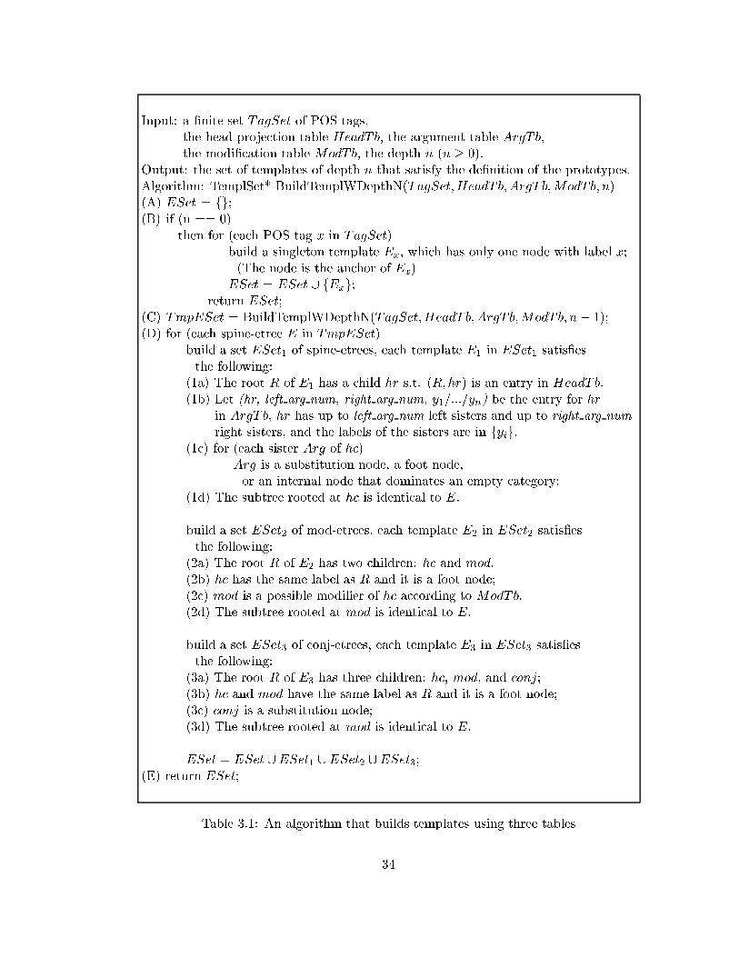
Input: a �nite set TagSet of POS tags,the head projection table HeadTb, the argument table ArgTb,the modi�cation table ModTb, the depth n (n � 0).
Output: the set of templates of depth n that satisfy the de�nition of the prototypes.Algorithm: TemplSet* BuildTemplWDepthN(TagSet;HeadTb;ArgTb;ModTb; n)(A) ESet = fg;(B) if (n == 0)
then for (each POS tag x in TagSet)build a singleton template Ex, which has only one node with label x;(The node is the anchor of Ex)
ESet = ESet [ fExg;return ESet;
(C) TmpESet = BuildTemplWDepthN(TagSet;HeadTb;ArgTb;ModTb; n� 1);(D) for (each spine-etree E in TmpESet)
build a set ESet1 of spine-etrees, each template E1 in ESet1 satis�esthe following:
(1a) The root R of E1 has a child hr s.t. (R; hr) is an entry in HeadTb.(1b) Let (hr, left arg num, right arg num, y1=:::=yn) be the entry for hr
in ArgTb, hr has up to left arg num left sisters and up to right arg numright sisters, and the labels of the sisters are in fyig.
(1c) for (each sister Arg of hc)Arg is a substitution node, a foot node,or an internal node that dominates an empty category;
(1d) The subtree rooted at hc is identical to E.
build a set ESet2 of mod-etrees, each template E2 in ESet2 satis�esthe following:
(2a) The root R of E2 has two children: hc and mod.(2b) hc has the same label as R and it is a foot node;(2c) mod is a possible modi�er of hc according to ModTb.(2d) The subtree rooted at mod is identical to E.
build a set ESet3 of conj-etrees, each template E3 in ESet3 satis�esthe following:
(3a) The root R of E3 has three children: hc, mod, and conj;(3b) hc and mod have the same label as R and it is a foot node;(3c) conj is a substitution node;(3d) The subtree rooted at mod is identical to E.
ESet = ESet [ESet1 [ESet2 [ESet3;(E) return ESet;
Table 3.1: An algorithm that builds templates using three tables
34
projected further according to HeadTb. Finally, G(n) (n > 3) is empty because G(3) does
not include any spine-etree. Now that we have an algorithm that calculates G(n) for any
integer n, we de�ne GTable to beSn2N G(n). GTable is the set of all possible templates
that satisfy the prototypes according to the three language-speci�c tables.
3.4 The problems with GTable
We have just shown that we can build a grammar GTable using three tables if we make
a certain assumption about syntactic variations (e.g., we assume that the only syntactic
variation in a language is that the arguments in a spine-etree can dominate empty cate-
gories). Given a natural language L, if the three tables for L are complete and error-free,
is GTable a good grammar for L? In other words, if GL is the ideal LTAG grammar for
the language L, is GTable a good approximation of GL? The answer is negative because
GTable overgenerates; that is, many templates in GTable are not in GL. In this section, we
discuss the sources of this overgeneration.
In Table 3.1, we wrote the algorithm as a recursive function. Conceptually, the algo-
rithm buildsGTable in four steps: �rst, it produces all possible spines according to the head
projection table; second, it adds arguments to the templates; third, for mod-etrees and
conj-etrees, the algorithm adds the top layer (i.e., a new root node and its children nodes);
fourth, it adds structures for syntactic variations. Each step may produce structures that
are not acceptable in language L.
� In the �rst step, the algorithm builds spines using a head projection table. When
people build LTAG grammars, they may use a label for more than one projection of
a head. For instance, both IP and CP nodes in GB theory have the label S in the
XTAG grammar. As a result, a label may appear on a spine more than once. For
instance, the label S appears twice on the spine for the template #2 in Figure 3.2.
In order to generate such template, the head projection table has to include entries
such as (S, S). Because of such an entry, the algorithm will produce spines with
an arbitrarily large number of S nodes; that is, the algorithm is not sophisticated
enough to know that the S label can appear once or twice on a spine, but not more
35
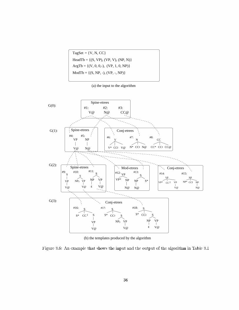
V*
V
CC V@
#6:
N*
N
N@CC
#7:
CC*
CC
CC CC@
#8:
S
VP
V@
S
VPNP
V@
CCS*
S S
S* CC
#18:
S
VPNP
V@ε
S
S* CC
#16: #17:
S
NP
N@
S*
VP
VP* NP
N@
#12:
Mod-etrees#13:
S
VPNP
V@
S
VP
V@
NP
NP
N@
CCNP*
VP
VP* VP
V@
CC
(a) the input to the algorithm
G(0):
G(1):
VP
V@
NP
N@
#4: #5:
Conj-etreesSpine-etrees
(b) the templates produced by the algorithm
G(2):
G(3): Conj-etrees
S
VPNP
V@ε
#11:Spine-etrees
#9: #10: #15:#14:
Conj-etrees
#2:V@
#1:N@ CC@
#3:
Spine-etrees
ModTb = {(S, NP, -), (VP, -, NP)}
ArgTb = {(V, 0, 0,-), (VP, 1, 0, NP)}
HeadTb = {(S, VP), (VP, V), (NP, N)}
TagSet = {V, N, CC}
Figure 3.6: An example that shows the input and the output of the algorithm in Table 3.1
36

VP
V@ NP
S
NP
NP
VP
V@
S
NP
NP
VP
V@
S
NPVP
V@ NP
S
NP
S S S S
#1: #2: #3: #4:
Figure 3.7: Among four of the templates in GTable for ditransitive verbs, the last two areimplausible.
than twice. As a result, the spines produced by the algorithm can be arbitrary long
and GTable is an in�nite set. Clearly, most of the spines and the templates with these
spines are implausible.
� In the second step, the algorithm adds zero or more arguments to the templates.
Let the argument table entry for a head hc be (hc, left max num, right max num,
y1=y2=::=yn), the algorithm tries every argument sequence that is consistent with
the entry.7 The number of such sequences is (Plm
i=0 ni) � (
Prmj=0 n
j), where ln is
left max num and rm is right max num. Not every sequence is plausible for language
L. For example, assuming that the argument table entry for English verbs is (V, 1,
2, NP/S), the algorithm will try all twenty-one argument sequences, but only ten
of them are actually allowed in English. The templates in Figure 3.7 show four of
the twenty-one argument sequences. They are (NP; NP, NP), (NP; NP, S), (NP;
S, NP), and (NP; S, S). Only the �rst two are allowed in English.
� In the third step, the algorithm adds a top layer for a mod-etree or a conj-etree. It
is possible, although not common, that the modi�ee may impose constraints on the
internal structure of the modi�er. For example, when an S modi�es an NP as in a
relative clause, exactly one constituent within the S must undergo wh-movement (see
templates #1 and #2 in Figure 3.8). Such constraints cannot be expressed in the
modi�cation table, As a result, GTable includes templates in which the constraints
are not satis�ed, such as #3 and #4 in Figure 3.8.
7An argument sequence is consistent with the entry if the number of left arguments in the sequence
is no more than left max num, the number of right arguments is no more than right max num, and each
argument has an label in fy1; y2; :::; yng.
37
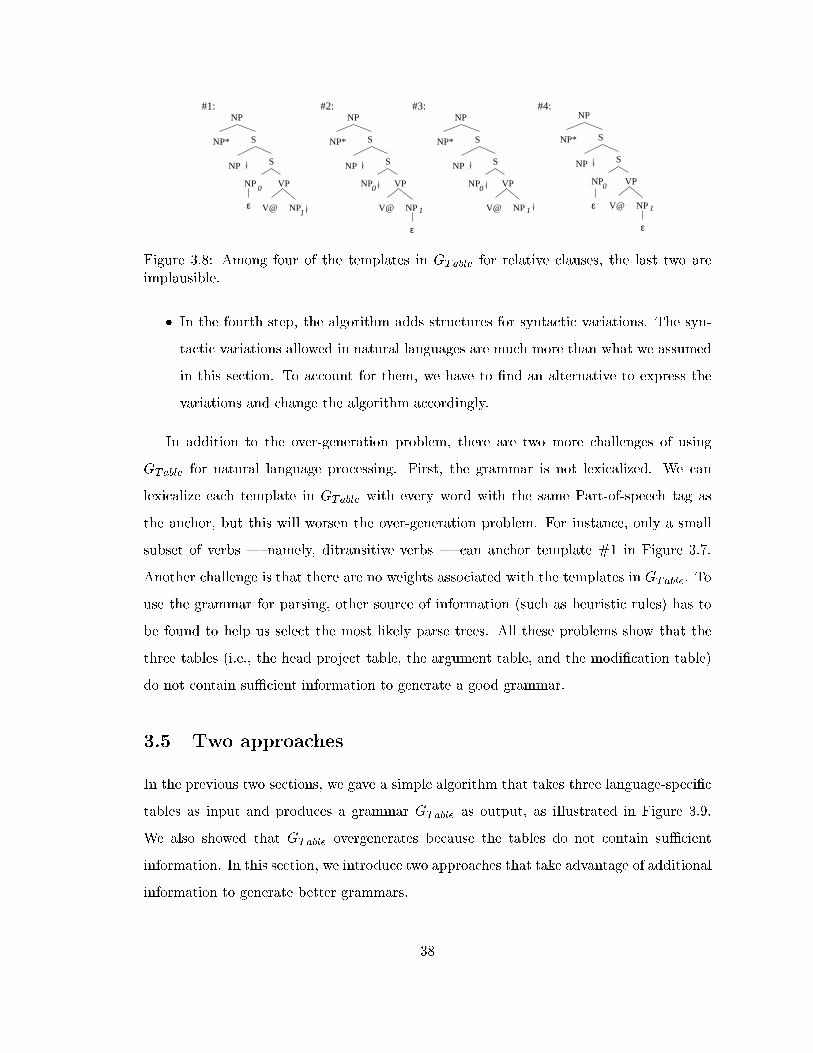
S
NPV@
NP
NP
VP
ε
NP
NP* S
#1: #3:#2:
1
0
S
NPV@
NP
NP
VP
NP
NP* S
ε
0
1
#4:
S
NPV@
NP
NP
VP
NP
NP* S
0
1
S
NPV@
NP
NP
VP
NP
NP* S
0
1ε
ε
Figure 3.8: Among four of the templates in GTable for relative clauses, the last two areimplausible.
� In the fourth step, the algorithm adds structures for syntactic variations. The syn-
tactic variations allowed in natural languages are much more than what we assumed
in this section. To account for them, we have to �nd an alternative to express the
variations and change the algorithm accordingly.
In addition to the over-generation problem, there are two more challenges of using
GTable for natural language processing. First, the grammar is not lexicalized. We can
lexicalize each template in GTable with every word with the same Part-of-speech tag as
the anchor, but this will worsen the over-generation problem. For instance, only a small
subset of verbs | namely, ditransitive verbs | can anchor template #1 in Figure 3.7.
Another challenge is that there are no weights associated with the templates in GTable. To
use the grammar for parsing, other source of information (such as heuristic rules) has to
be found to help us select the most likely parse trees. All these problems show that the
three tables (i.e., the head project table, the argument table, and the modi�cation table)
do not contain suÆcient information to generate a good grammar.
3.5 Two approaches
In the previous two sections, we gave a simple algorithm that takes three language-speci�c
tables as input and produces a grammar GTable as output, as illustrated in Figure 3.9.
We also showed that GTable overgenerates because the tables do not contain suÆcient
information. In this section, we introduce two approaches that take advantage of additional
information to generate better grammars.
38
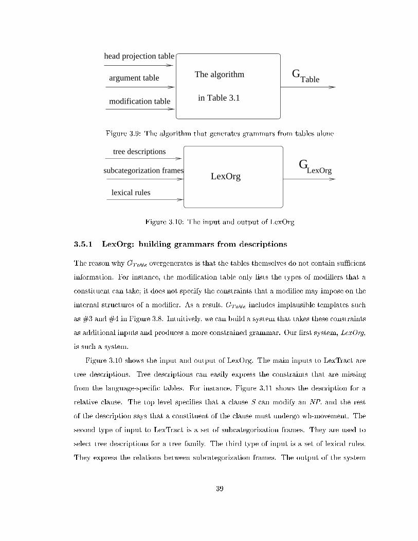
in Table 3.1
The algorithm
modification table
argument table
head projection table
GTable
Figure 3.9: The algorithm that generates grammars from tables alone
subcategorization frames
tree descriptions
lexical rules
LexOrgG
LexOrg
Figure 3.10: The input and output of LexOrg
3.5.1 LexOrg: building grammars from descriptions
The reason why GTable overgenerates is that the tables themselves do not contain suÆcient
information. For instance, the modi�cation table only lists the types of modi�ers that a
constituent can take; it does not specify the constraints that a modi�ee may impose on the
internal structures of a modi�er. As a result, GTable includes implausible templates such
as #3 and #4 in Figure 3.8. Intuitively, we can build a system that takes these constraints
as additional inputs and produces a more constrained grammar. Our �rst system, LexOrg,
is such a system.
Figure 3.10 shows the input and output of LexOrg. The main inputs to LexTract are
tree descriptions. Tree descriptions can easily express the constraints that are missing
from the language-speci�c tables. For instance, Figure 3.11 shows the description for a
relative clause. The top level speci�es that a clause S can modify an NP, and the rest
of the description says that a constituent of the clause must undergo wh-movement. The
second type of input to LexTract is a set of subcategorization frames. They are used to
select tree descriptions for a tree family. The third type of input is a set of lexical rules.
They express the relations between subcategorization frames. The output of the system
39

NPS
NP S
NP
ε
NP*
Figure 3.11: Tree description for a relative clause
The algorithm
in Table 3.1
GTable
G *Table
a filter
LexTract
head projection table
modification table
argument table
a treebank
Figure 3.12: The conceptual approach of LexTract
is a grammar GLexOrg, which is a subset of GTable and should not include implausible
templates.8 In chapter 4, we shall describe this system in detail.
3.5.2 LexTract: extracting grammars from Treebanks
In LexOrg, the overgeneration problem is solved by adding more information to the input.
An alternative is to keep the input intact but add a new module which chooses a subset
of GTable. Our second system, named LexTract, uses this alternative.
As shown in Figure 3.12, the inputs to LexTract are three language-speci�c tables and
a Treebank. Conceptually, LexTract �rst uses the tables to generate GTable, then uses the
Treebank to select a subset G�Table of GTable such that each template in the subset is used at
least once to produce correct derived trees for the grammatical sentences in the Treebank.
It is obvious that G�Table is a subset of GL. If a Treebank included all the grammatical
8It goes without saying that the quality of GLexOrg depends on the quality of the input to LexOrg.
40

G
G
GTable
L
Table*
Figure 3.13: The relations between GTable, GL and G�Table
sentences for a language L, G�Table would be identical to GL. In reality, a Treebank is �nite
and therefore cannot include all the grammatical sentences. Nevertheless, if a Treebank
is a good representative of a language itself, G�Table is a good approximation of GL. The
relation between GTable, GL and G�Table are shown in Figure 3.13. The better a Treebank
is, the closer G�Table is to GL. In Chapter 5, we describe LexTract in detail.
3.6 Summary
In this chapter, we �rst discuss four types of information that should be included in el-
ementary trees: the head and its projections. the arguments of the head, the modi�ers
of the head, and syntactic variations. Then we de�ne three forms of elementary trees in
our target grammar: spine-etrees, mod-etrees, and conj-etrees. Next we describe a sim-
ple algorithm that takes three language-speci�c tables as input and produces a grammar
GTable as output. The grammar overgenerates because the tables do not contain suÆcient
information. Finally, we give an overview of two systems that address this overgeneration
problem: the �rst system (LexOrg) overcomes the problem by requiring additional infor-
mation from the input; the second system (LexTract) uses a Treebank as a �lter to choose
a subset of GTable. The details of the systems are covered in the next two chapters.
41
Chapter 4
LexOrg: a system that builds
LTAGs from descriptions
Elementary trees in an LTAG grammar often share some common structures. The reuse
of the common structures creates redundancy. This redundancy problem was addressed
in several previous works, including (Vijay-Shanker and Schabes, 1992), (Becker, 1994),
(Evans et al., 1995), and (Candito, 1996). In (Vijay-Shanker and Schabes, 1992), Vijay-
Shanker and Schabes presented a scheme for eÆciently representing an LTAG grammar
using descriptions (a.k.a. tree descriptions or descriptions of trees). We extended the
concept of descriptions and built a system, called LexOrg, that generates templates from
a set of descriptions.1 2
The chapter is organized as follows: In Section 4.1, we describe the problems caused by
the reuse of structures among templates. In Section 4.2, we introduce the overall approach
of LexOrg. In Section 4.3, we de�ne the notions of descriptions and trees in a simpli�ed
�rst-order logic. In Section 4.4, we introduce four types of descriptions. In Sections 4.5 {
4.7, we discuss three components of LexOrg. In Section 4.8, we report our experiments on
1LexOrg produces elementary trees exactly the same way as it produces templates. In this chapter,
very often we use the term trees to refer to structures in a simpli�ed �rst-order logic (see Table 4.4). To
prevent the potential confusion between trees as structures and trees as elementary trees, we shall discuss
the generation of templates, rather than the generation of elementary trees.
2Our previous work on LexOrg can be found in (Xia et al., 1998) and (Xia et al., 1999).
42

0
NP
VP
1
NPNP
NP
S
ε
VP
NP
0
V@
#2:
S NP S
V@1
NP1
0
V@
ε
#3:
S
S
VP1
V@
NP VP
S
NP
Transitive verbs: (NP0 V NP1)
#1: #4:
Ergative verbs: (NP1 V)
NP
S
ε
S
NP VP
VP
VP* S
VP
ε
NP
1
V@
1
V@
#5: #7:#6:
VP
VP* S
0 VP
NPε
NP
1V@
Figure 4.1: Templates in two tree families
using LexOrg to generate grammars for English and Chinese. In Section 4.9, we discuss
how the users of LexOrg can create the input to LexOrg. In Section 4.10, we compare
LexOrg with related work. In Section 4.11, we summarize the whole chapter.
4.1 Structure sharing among templates
The templates in an LTAG grammar often share some common structures. Figure 4.1
shows seven templates for ergative verbs such as break. The top four templates show the
syntactic environments for ergative verbs when they act as transitive verbs, such as break
in He broke two windows. #1 is for a declarative sentence, #2 and #3 are for wh-questions,
and #4 is for a purpose clause.3 There are two templates for wh-questions because the
moved constituent can be either the subject (as in #2) or the object (as in #3). The
bottom three templates show the syntactic environments for ergative verbs when they act
as intransitive verbs, such as break in The window broke.
Among the seven templates in Figure 4.1, #1, #2, #3, and #4 all have the structure
in Figure 4.2(a), templates #2, #3, and #6 have the structure in Figure 4.2(b), templates
#4 and #7 have the structure in Figure 4.2(c), and so on. The dashed line in Figure 4.2(b)
3Template #4 is anchored by a verb such as please in the sentence John bought a book to please Mary,
where the subordinating clause to please Mary modi�es the verb phrase bought a book in the matrix clause.
43
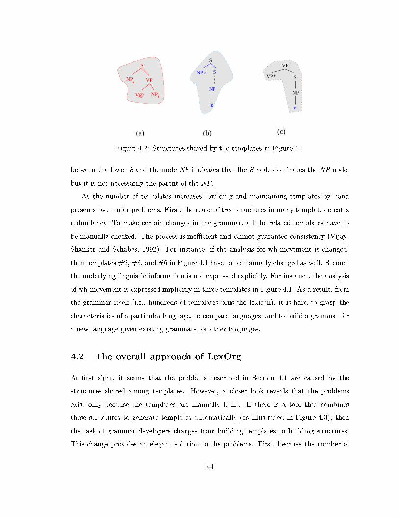
S
0VP
NP1V@
NP SVP*
NP
ε
VP
(b)(a)
NP
ε
NP
S
S
(c)
Figure 4.2: Structures shared by the templates in Figure 4.1
between the lower S and the node NP indicates that the S node dominates the NP node,
but it is not necessarily the parent of the NP.
As the number of templates increases, building and maintaining templates by hand
presents two major problems. First, the reuse of tree structures in many templates creates
redundancy. To make certain changes in the grammar, all the related templates have to
be manually checked. The process is ineÆcient and cannot guarantee consistency (Vijay-
Shanker and Schabes, 1992). For instance, if the analysis for wh-movement is changed,
then templates #2, #3, and #6 in Figure 4.1 have to be manually changed as well. Second,
the underlying linguistic information is not expressed explicitly. For instance, the analysis
of wh-movement is expressed implicitly in three templates in Figure 4.1. As a result, from
the grammar itself (i.e., hundreds of templates plus the lexicon), it is hard to grasp the
characteristics of a particular language, to compare languages, and to build a grammar for
a new language given existing grammars for other languages.
4.2 The overall approach of LexOrg
At �rst sight, it seems that the problems described in Section 4.1 are caused by the
structures shared among templates. However, a closer look reveals that the problems
exist only because the templates are manually built. If there is a tool that combines
these structures to generate templates automatically (as illustrated in Figure 4.3), then
the task of grammar developers changes from building templates to building structures.
This change provides an elegant solution to the problems. First, because the number of
44

S
0VPNP
1NPV@
NP
ε
NP
S
S
VP
NP1
S
0
NP
ε
NP
V@
S
(b)(a) (c)
Figure 4.3: Combining descriptions to generate templates
GeneratorFrame Description
Selector
framedescriptions
sets of
GeneratorTree
templates
descriptions
a subcatframessubcat
lexical rules
Figure 4.4: The architecture of LexOrg
these structures is much less than that of the templates, and the structures are smaller
and simplier than templates, the grammar development time will be reduced. If grammar
developers want to change the analysis of a certain phenomenon (e.g., wh-movement), they
need to modify only the structure that represents the phenomenon (e.g., the structure in
Figure 4.3(b) for wh-movement). LexOrg will propagate the modi�cation in the structure
to all the templates that subsume the structure. Therefore, the templates are consistent.
Second, the underlying linguistic information (such as wh-movement) is expressed explicitly
as a structure, so it is easy to grasp the main characteristics of a language, to compare
languages, and so on.
Based on this intuition, we built a system, LexOrg, which combines tree structures to
generate templates. Following (Vijay-Shanker and Schabes, 1992), we represent the shared
structures as descriptions. The inputs to LexOrg are a set of subcategorization frames, a
�nite set of lexical rules, and a �nite set of descriptions. As shown in Figure 4.4, LexOrg
has three components: a Frame Generator, a Description Selector, and a Tree Generator.
For each subcategorization frame fr that is a member of the input subcategorization
frames, the Frame Generator applies the set of input lexical rules to it and builds a set of
subcategorization frames that are related to fr. For each subcategorization frame produced
45

by the Frame Generator, the Description Selector chooses a subset of the input description
set. For each subset of descriptions, the Tree Generator combines the descriptions in
the subset to produce a set of templates. Therefore, the outputs of LexOrg are a set of
templates for fr and all the subcategorization frames that are derived from fr by applying
lexical rules. In the following sections, we �rst de�ne the notions of descriptions and trees,
then discuss each component of LexOrg in detail.4
4.3 The de�nition of a description
Vijay-Shanker and Schabes (1992) presented a scheme for eÆciently representing an LTAG
grammar using descriptions. Rogers and Vijay-Shanker (1994) later gave a formal de�-
nition of description. We extend their de�nition to include feature structures. In this
section, we �rst give a brief introduction to these two pieces of work, then introduce our
extended de�nition of description that is used in LexOrg.
4.3.1 A compact representation of LTAG grammars
Vijay-Shanker and Schabes (1992) presented a scheme for eÆciently representing an LTAG
grammar using descriptions. The scheme adopts two mechanisms. The �rst mechanism is
the use of hierarchy for lexical entries, a fragment of which is shown in Figure 4.5. The
value of an attribute of a lexical entry in the lexicon is either obtained by inheritance or
by local speci�cation. A class in a hierarchy (such as DITRANS-1) may have more than
one superclass, and the local speci�cation can overwrite inherited attributes. Figure 4.6
shows the lexicon entries for six classes of verbs; namely, VERB, TRANSITIVE, IOBJ,
NP-IOBJ, PP-IOBJ, and DITRANS1.5
The second mechanism is the use of lexical and syntactic rules to capture in ectional
4To make it easier for readers to understand the system, we describe the three components of LexOrg
in reverse order; that is, we cover the Tree Generator �rst, then the Description Selector, and �nally the
Frame Generator.5A class is an abstract data type. The notion of class in this context is more similar to the notion of
class in a program language such as C++ than to that of verb class in (Levin, 1993).
46

TRANSITIVE BQUI INTRANSITIVE
PP-IOBJ NP-IOBJ
DITRANS-1 DITRANS-2 OBJ-BQUI SIMPLE-TRANS
IOBJ
VERB
eatgive donate
Figure 4.5: The fragment of the lexicon given in (Vijay-shanker & Schabes, 1992)
v np
vp
v = head-daughter(vp)anchor = v
s = completion(v)arg: npconstraints equations: ....
superclasses: VERBnodes: vp, v, np
description:
TRANSITIVE
vp
v np
constraints equations: ...arg: npanchor = v
description:
nodes: vp, v, np
superclasses: VERB
IOBJ
PP-IOBJ
superclasses: IOBJnodes: vp, v, pp, p, np
description: vp
v pp
p npconstraints equations: ....arg: ppnp = arg(IOBJ)anchor = v
DITRANS1
superclasses: TRANSITIVE, PP-IOBJ
LP: arg(TRANSITIVE) < arg(PP-IOBJ)
constraints equation: { s.<cat> = Snp.<agr> = vp.<arg>np.<case> = nom
...
description:
s
np vp
v
vp = head-daughter(s)
np < vpanchor = v
s = completion(v)agr: np
NP-IOBJ
superclasses: IOBJ
description: vp
npvconstraints equations: ...arg: np
anchor = vnp = arg(IOBJ)
nodes: vp, v, np
VERB
nodes: s, np, vp, v
(d) (e) (f)
(a) (b) (c)
Figure 4.6: The de�nition of six verb classes given in (Vijay-shanker & Schabes, 1992)
47

args(LE )i
output: LEo
LE .tree-description = x’
S
S
y
x
ε
o
input: LEi
v (pp)
vp
by
npp
LE .tree-descriptiono
passive LE .CLASSESo
output: LEo
input: LEi
y = completion (LEi )x’ = copy(x)
x
WH-QUESTION PASSIVE
LE .CLASSESoLE .CLASSESoLE .CLASSi
CHANGE-ARITY(LE .CLASS) i
(a) (b)
Figure 4.7: Rules to handle wh-movement and passive
and derivational relationships among lexical entries. Figure 4.7 shows the rules for wh-
question and passive. The rules may make reference to the class hierarchy. For instance,
the passive rule uses the CHANGE ARITY relation, where C2 = CHANGE�ARITY (C1)
means that C2 is the immediate superclass of C1 distinct from TRANSITIVE.
Both mechanisms make use of descriptions. In a description, a dashed line from node
a to b means that a dominates b; a solid line means that a is the parent of b. Descriptions
di�er from trees in that descriptions can leave things underspeci�ed. This underspeci�ca-
tion is desirable because we want descriptions to be general enough. For instance, in the
description of the class IOBJ (see Figure 4.6(c)), the vp node dominates the np, but it is
not necessarily the parent of np. Leaving the number of intermediate nodes between vp
and np underspeci�ed makes the relation between them hold in both of IOBJ's subclasses:
in NP-IOBJ, the vp is the parent of the np; in PP-IOBJ, it is the grandparent of the
np. Similarly, in the description for wh-movement as shown in Figure 4.8(a), the node S1
dominates NP1. The description is general enough to cover both cases in Figure 4.8(b)
and (c). In the former case, NP1 is the subject of the sentence and a child of S1; in the
latter case, NP1 is the object of the sentence and a grandchild of S1.
48
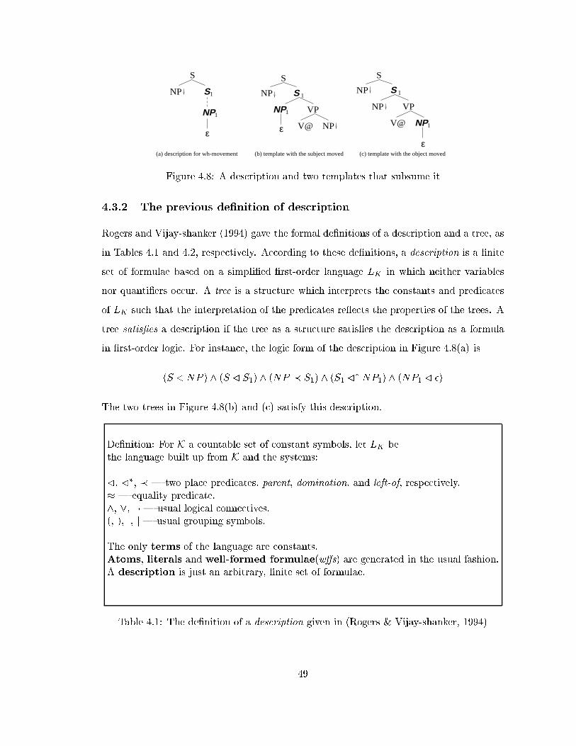
S
NP
ε
NP
1
1
S
VP
NP
S
NP
ε V@
S
NP1
1
VP
S
NP
ε
V@
NP
S
NP1
1
(a) description for wh-movement (b) template with the subject moved (c) template with the object moved
Figure 4.8: A description and two templates that subsume it
4.3.2 The previous de�nition of description
Rogers and Vijay-shanker (1994) gave the formal de�nitions of a description and a tree, as
in Tables 4.1 and 4.2, respectively. According to these de�nitions, a description is a �nite
set of formulae based on a simpli�ed �rst-order language LK in which neither variables
nor quanti�ers occur. A tree is a structure which interprets the constants and predicates
of LK such that the interpretation of the predicates re ects the properties of the trees. A
tree satis�es a description if the tree as a structure satis�es the description as a formula
in �rst-order logic. For instance, the logic form of the description in Figure 4.8(a) is
(S �NP ) ^ (S � S1) ^ (NP � S1) ^ (S1 �� NP1) ^ (NP1 � �)
The two trees in Figure 4.8(b) and (c) satisfy this description.
De�nition: For K a countable set of constant symbols, let LK bethe language built up from K and the systems:
�, ��, � | two place predicates, parent, domination, and left-of, respectively.� | equality predicate.^, _, : | usual logical connectives.(, ), [, ] | usual grouping symbols.
The only terms of the language are constants.Atoms, literals and well-formed formulae(w�s) are generated in the usual fashion.A description is just an arbitrary, �nite set of formulae.
Table 4.1: The de�nition of a description given in (Rogers & Vijay-shanker, 1994)
49

De�nition: For any language LK , a model for LK is a tuple (U ; I;P;D;L), whereU is a nonempty universe,I is a function from K to U ,P;D;L are binary relations over U (interpreting �, ��, �, respectively).
A tree is a model satisfying the conditions:(I) For some R 2 U and all w; x; y; z 2 U ,
/* T1 requires a tree to have a root */T1: (R; x) 2 D
/* T2 | T4 require the domination relation to be re exive,anti-symmetric, and transitive */
T2: (x; x) 2 DT3: (x; y); (y; x) 2 D ) x = yT4: (x; y); (y; z) 2 D ) (x; z) 2 D
/* T5 | T7 relate the parent and domination relations */T5: (x; y) 2 P ) [(x; y) 2 D and (y; x) 62 D]T6: [(x; z) 2 P and (x; y); (y; z) 2 D]) [(x = y or (y = z)]T7: (x; y) 2 D ) (y; x) 2 D or
(9x0; y0)[(x; x0); (y0; y) 2 P and (x; y0); (x0; y) 2 D]
/* T8 | T10 relate the domination and left-of relations */T8: (x; y) 2 D or (y; x) 2 D or (x; y) 2 L or (y; x) 2 LT9: (x; y) 2 L ) (x; y) 62 D; (y; x) 62 D; and (y; x) 62 LT10: [(x; y) 2 L and (x;w); (y; z) 2 D]) (w; z) 2 L
/* T11 requires the left-of relation to be transitive */T11: (x; y); (y; z) 2 L ) (x; z) 2 L
(II) For every x 2 U , the setsBx = fy j (y; x) 2 Dg andLx = fy j (9z)[(z; y); (z; x) 2 P and (y; x) 2 L]gare �nite.
Table 4.2: The de�nition of a tree given in (Rogers & Vijay-shanker, 1994)
50

4.3.3 The de�nition of descriptions in LexOrg
When we built LexOrg, we extended the previous de�nitions of descriptions and trees.
The new de�nition of description
The major extension that we made to the previous de�nition is that we now include feature
structures. This extension is necessary for three reasons. First, in the LTAG formalism, fea-
ture structures are associated with the nodes in a template to specify linguistic constraints
(see Section 2.1.5). They should be included in descriptions so that when descriptions are
combined by LexOrg, the features are carried over to the resulting templates. Second, in
addition to features appearing in templates, each node in a description has three special
features. The �rst one, cat, is the category of the node. The second feature, type, is the
type of the node. The feature has four possible values: an internal node, a foot node, an
anchor node, or a substitution node. The third feature subsc is the subscript of the node.
An LTAG grammar may use subscripts to distinguish the nodes in a template with the
same category. For instance, it may name the subject NP0 and the object NP1. The third
reason why we include features in descriptions is that LexOrg can use feature uni�cation
to rule out incompatible combinations of descriptions (see Section 4.5). The new de�nition
of description is shown in Table 4.3. In the new de�nition, an atomic formula is either an
atomic formula in the original de�nition or is a feature equation, and a description is a w�
rather than a �nite set of w�s.
Figure 4.9 shows two ways of representing the same description: the left one is in the
logical form; the right one is a graph, in which the features of nodes (including the cate-
gories of nodes) are enclosed in parentheses. The graphic representation is more intuitive
and easier to read, but not every description can be displayed as a graph because a de-
scription may use negation and disjunctive connectives. In the following sections, we shall
use the graphical representation when possible and use the logic representation in other
cases.
51

De�nition: For K a countable set of constant symbols,let L
Kbe the language built up from K and the systems:
�, ��, � | two place predicates, parent, domination, and left-of, respectively.� | equality predicate.^, _, : | usual logical connectives.(, ), [, ] | usual grouping symbols.F | a �nite set of feature names.V | a �nite set of feature values.cat, type, subsc | three features in F .
cat is the syntactic category (e.g., S, NP ) of a node,type is the type of a node (e.g., internal node, foot node, and anchor node).subsc is the subscript of the node.
� | the empty category, one of the values in V for the feature cat.internal, foot, anchor, and subst | four values in V for the feature type.
The only terms of the language are constants.
An atomic formula is one of the following:(1) t12t2, where 2 is �, ��, or �, and t1 and t2 are terms.(2) t:f = v, where t is a term, f 2 F , and v 2 V.(3) t1:f1 = t2:f2, where t1 and t2 are terms, and f1, f2 2 F .
Well-formed formulae(w�s) are generated in the usual fashion.
A description is a w�.
Table 4.3: The new de�nition of description used in LexOrg
(a) the logical representation
S
NP S
NP
0
0
1
1
(’S’)
(’S’)
(’NP’)
(’NP’)
(b) the graphical representation
Trace (’ε’)
(S0 �NP0) ^ (S0 � S1)^(NP0 � S1) ^ (S1 �
� NP1)^(NP1 � �) ^ (S0:label =
0 S0)^(NP0:label =
0 NP 0) ^ (S1:label =0 S0)
^(NP1:label =0 NP 0) ^ (Trace:label =0 �0)
Figure 4.9: Two representations of a description
52
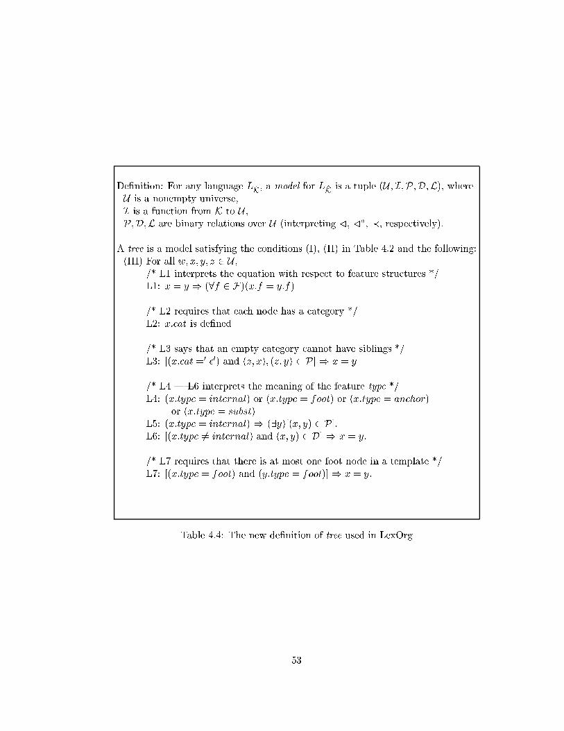
De�nition: For any language LK, a model for LK is a tuple (U ; I;P;D;L), whereU is a nonempty universe,I is a function from K to U ,P;D;L are binary relations over U (interpreting �, ��, �, respectively).
A tree is a model satisfying the conditions (I), (II) in Table 4.2 and the following:(III) For all w; x; y; z 2 U ,
/* L1 interprets the equation with respect to feature structures */L1: x = y ) (8f 2 F)(x:f = y:f)
/* L2 requires that each node has a category */L2: x:cat is de�ned
/* L3 says that an empty category cannot have siblings */L3: [(x:cat =0 �0) and (z; x); (z; y) 2 P] ) x = y
/* L4 | L6 interprets the meaning of the feature type */L4: (x:type = internal) or (x:type = foot) or (x:type = anchor)
or (x:type = subst)L5: (x:type = internal) ) (9y)[(x; y) 2 P].L6: [(x:type 6= internal) and (x; y) 2 D] ) x = y.
/* L7 requires that there is at most one foot node in a template */L7: [(x:type = foot) and (y:type = foot)] ) x = y.
Table 4.4: The new de�nition of tree used in LexOrg
53

The new de�nition of tree
Now that we have extended the de�nition of description, the de�nition of tree needs to be
revised as well. The new de�nition is in Table 4.4. Under this new de�nition, each node in
U is associated with a feature structure. For each feature in the feature structure, there are
three possibilities for its value: (1) the feature value is not de�ned; (2) the feature value
is equal to one of the constants in V; (3) the feature value is equal to the feature value ofanother node. A tree is a model if it satis�es all the conditions in the original de�nition
plus the additional requirements L1 | L7. L1 says that, if two nodes are equal, all the
features of the nodes should have the same values. L2 requires each node to be assigned
a category. L3 says that an empty category cannot have any sibling. L4 | L6 give the
interpretation of four types of nodes: a node in a tree is either an internal node or a leaf
node; a leaf node is a foot or an anchor or a substitution node. L7 says that each tree
has at most one foot node.
This de�nition of tree is closely related to the traditional de�nition of rooted, ordered
tree. To avoid confusion, in this chapter, we use trees to refer to the former, and rooted,
ordered trees to the latter. The de�nition of tree in LexOrg is more complicated than the
traditional de�nition of rooted, ordered trees. First, each node in a tree is associated with
a feature structure. Second, a tree has a component I, which is a function from K to U .6
Given a tree T = (U ;I;P;D;L), we can draw a graphic tree T as follows:
� For every x 2 U , build a unique node x in T .
� The edge (x; y) is in T if and only if (x,y) is a pair in P.
� The node x appears to the left of y in T if and only if (x; y) is in L.
To represent the function I and features in T , we write the node x in the form
fkig(ffm = vmg), where fkig is a subset of K such that I(ki) = x; that is, x represents the
set of symbols in K that map to x. For any kj in fkig, if kj :fm is equal to vm, we include
fm = vm in the parentheses. We often omit the curly brackets and all the features but cat
6If two nodes in K map to the same node in U , it means that these two nodes which appear in descriptionsare merged into a single node in the templates that are derived from the descriptions.
54
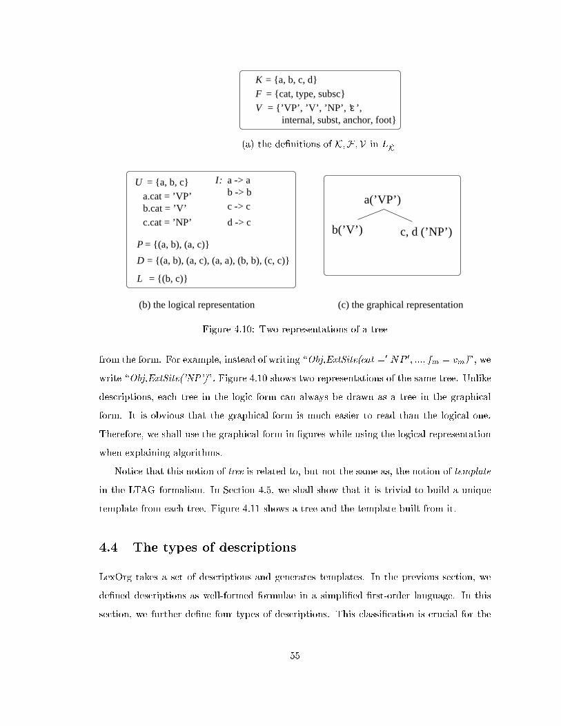
b -> b
c -> c
I: a -> a
d -> c
= {(a, b), (a, c)}
= {(a, b), (a, c), (a, a), (b, b), (c, c)}
= {(b, c)}
P
D
L
a(’VP’)
b(’V’) c, d (’NP’)
internal, subst, anchor, foot}
(b) the logical representation (c) the graphical representation
= {a, b, c, d}
= {cat, type, subsc}
= {’VP’, ’V’, ’NP’, ’
FK
V ε ’,
= {a, b, c}
a.cat = ’VP’b.cat = ’V’
c.cat = ’NP’
U
(a) the de�nitions of K;F ;V in LK
Figure 4.10: Two representations of a tree
from the form. For example, instead of writing \Obj,ExtSite(cat =0 NP 0; :::; fm = vm)", we
write \Obj,ExtSite('NP')". Figure 4.10 shows two representations of the same tree. Unlike
descriptions, each tree in the logic form can always be drawn as a tree in the graphical
form. It is obvious that the graphical form is much easier to read than the logical one.
Therefore, we shall use the graphical form in �gures while using the logical representation
when explaining algorithms.
Notice that this notion of tree is related to, but not the same as, the notion of template
in the LTAG formalism. In Section 4.5, we shall show that it is trivial to build a unique
template from each tree. Figure 4.11 shows a tree and the template built from it.
4.4 The types of descriptions
LexOrg takes a set of descriptions and generates templates. In the previous section, we
de�ned descriptions as well-formed formulae in a simpli�ed �rst-order language. In this
section, we further de�ne four types of descriptions. This classi�cation is crucial for the
55
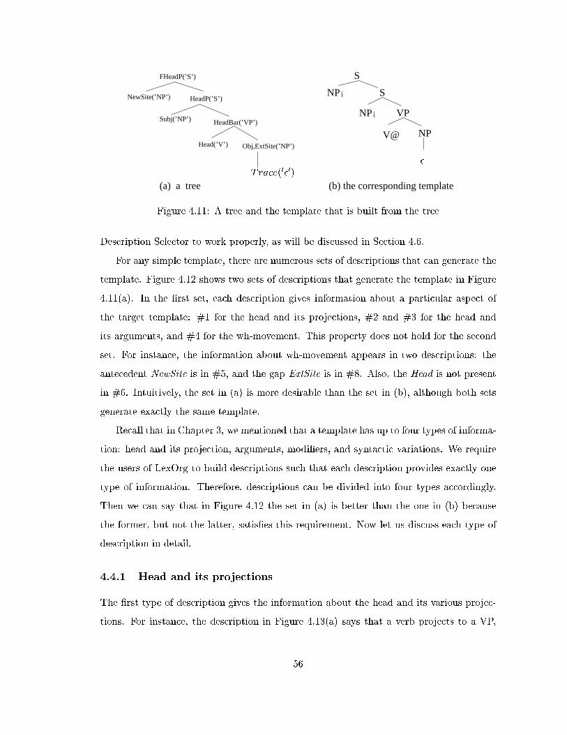
Subj(’NP’) HeadBar(’VP’)
Head(’V’) Obj,ExtSite(’NP’)
HeadP(’S’)NewSite(’NP’)
FHeadP(’S’)
(a) a tree (b) the corresponding template
S
NP S
NP VP
NPV@
Trace(0�0)�
Figure 4.11: A tree and the template that is built from the tree
Description Selector to work properly, as will be discussed in Section 4.6.
For any simple template, there are numerous sets of descriptions that can generate the
template. Figure 4.12 shows two sets of descriptions that generate the template in Figure
4.11(a). In the �rst set, each description gives information about a particular aspect of
the target template: #1 for the head and its projections, #2 and #3 for the head and
its arguments, and #4 for the wh-movement. This property does not hold for the second
set. For instance, the information about wh-movement appears in two descriptions: the
antecedent NewSite is in #5, and the gap ExtSite is in #8. Also, the Head is not present
in #6. Intuitively, the set in (a) is more desirable than the set in (b), although both sets
generate exactly the same template.
Recall that in Chapter 3, we mentioned that a template has up to four types of informa-
tion: head and its projection, arguments, modi�ers, and syntactic variations. We require
the users of LexOrg to build descriptions such that each description provides exactly one
type of information. Therefore, descriptions can be divided into four types accordingly.
Then we can say that in Figure 4.12 the set in (a) is better than the one in (b) because
the former, but not the latter, satis�es this requirement. Now let us discuss each type of
description in detail.
4.4.1 Head and its projections
The �rst type of description gives the information about the head and its various projec-
tions. For instance, the description in Figure 4.13(a) says that a verb projects to a VP,
56

HeadP(’S’)
HeadBar(’VP’)
Head(’V’)
HeadP
HeadBarSubj(’NP’)
HeadBar
Head Obj(’NP’)
FHeadP
HeadP(’S’)
HeadBar
HeadBar
Head Obj(’NP’)
#1: #4:#3:#2:
(a) a more desirable set
(b) a less desirable set
FHead(’S’)
NewSite HeadP(’S’)
ExtSite
#5: #6: #7:
HeadP
Subj(’NP’)
Head(’V’)
#9:#8:
FHeadP(’S’)
NewSite
HeadBar(’VP’)
ExtSite
HeadP
Trace(0�0)
Trace(0�0)
Figure 4.12: Two sets of descriptions that generate the same tree
and the VP projects to an S. In this chapter,
4.4.2 Arguments of a head
The second type of description speci�es the number, the types, and the positions of argu-
ments that a head can take, and the constraints that a head imposes on its arguments. For
instance, the description in Figure 4.13(b) says that the subject | a left argument of the
head | is a sister of the HeadBar. The feature equation in the description ensures that the
subject and the HeadBar must agree on numbers, persons, and so on. The description in
Figure 4.13(c) says that a head can take a right argument, which appears as a sister of the
head. Combining the descriptions for the �rst two types forms a description for the whole
subcategorization frame, as in Figure 4.13(d); therefore, we use the term subcategorization
descriptions to refer to descriptions in either the �rst or the second type.
4.4.3 Modi�ers of a head
The third type of description speci�es the type and the position of a modi�er with respect to
the modi�ee, and any constraint on the modi�cation relation. For instance, the description
57
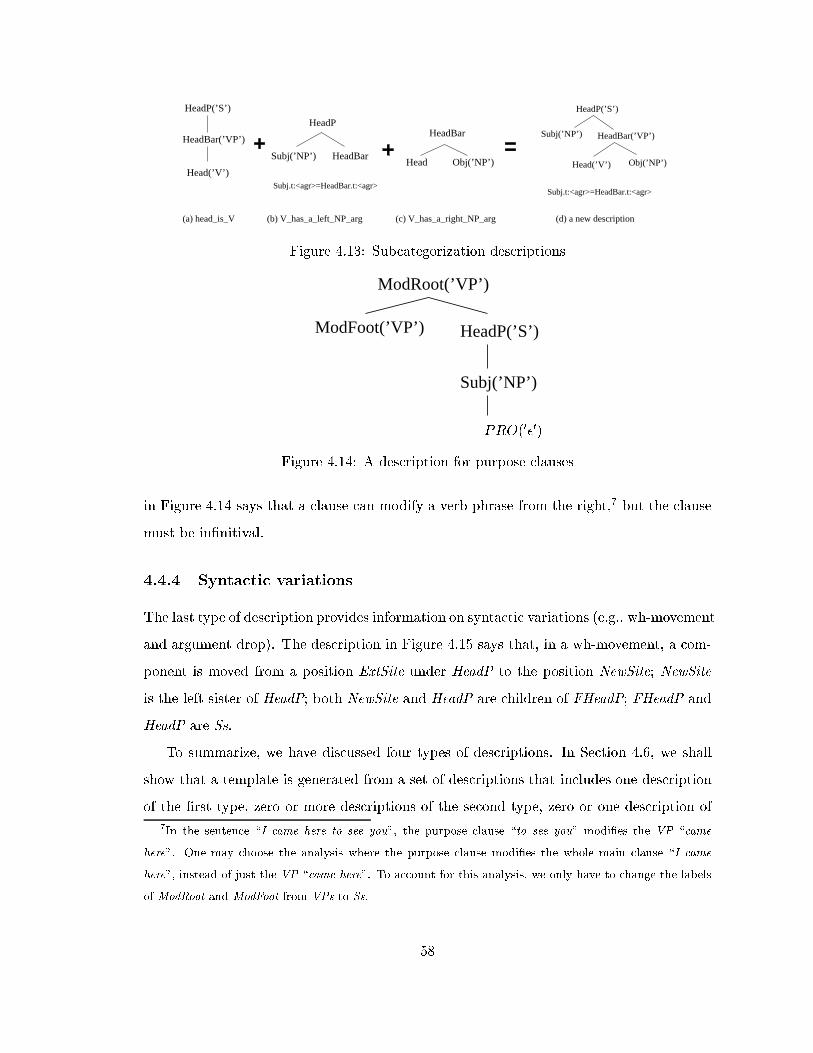
HeadP(’S’)
HeadBar(’VP’)
Head(’V’)
Subj(’NP’) HeadBar
HeadP
HeadP(’S’)
Head(’V’) Obj(’NP’)
Subj(’NP’) HeadBar(’VP’)
Subj.t:<agr>=HeadBar.t:<agr>
Obj(’NP’)
HeadBar
Head
Subj.t:<agr>=HeadBar.t:<agr>
(c) V_has_a_right_NP_arg(b) V_has_a_left_NP_arg(a) head_is_V (d) a new description
Figure 4.13: Subcategorization descriptions
ModFoot(’VP’)
ModRoot(’VP’)
HeadP(’S’)
Subj(’NP’)
PRO(0�0)
Figure 4.14: A description for purpose clauses
in Figure 4.14 says that a clause can modify a verb phrase from the right,7 but the clause
must be in�nitival.
4.4.4 Syntactic variations
The last type of description provides information on syntactic variations (e.g., wh-movement
and argument drop). The description in Figure 4.15 says that, in a wh-movement, a com-
ponent is moved from a position ExtSite under HeadP to the position NewSite; NewSite
is the left sister of HeadP; both NewSite and HeadP are children of FHeadP; FHeadP and
HeadP are Ss.
To summarize, we have discussed four types of descriptions. In Section 4.6, we shall
show that a template is generated from a set of descriptions that includes one description
of the �rst type, zero or more descriptions of the second type, zero or one description of
7In the sentence \I came here to see you", the purpose clause \to see you" modi�es the VP \came
here". One may choose the analysis where the purpose clause modi�es the whole main clause \I came
here", instead of just the VP \came here". To account for this analysis, we only have to change the labels
of ModRoot and ModFoot from VPs to Ss.
58

FHeadP(’S’)
HeadP(’S’)NewSite
ExtSite
Trace(0�0)
Figure 4.15: A description for wh-movement
the third type, and zero or more descriptions of the last type.
4.5 The Tree Generator
The most complicated component of LexOrg is called Tree Generator (TreeGen). The
function of the Tree Generator is to take a set of descriptions as input, and generate
templates as output. This is done in three steps: �rst, TreeGen combines the input set of
descriptions to get a new description; second, TreeGen builds a set of trees such that each
tree in the set satis�es the new description and has the minimal number of nodes; third,
TreeGen builds a template for each tree in the set. In Figure 4.16, the descriptions in (a)
are the input to TreeGen. The new description is in (b). Notice that in (b) the position
of ExtSite with respect to Subj and HeadBar is not speci�ed. There are many trees that
satisfy this description, but the two trees in (c) are the only ones with the minimal number
of nodes. From these two trees, TreeGen builds two templates in (d). In this section, we
explain each step in detail.
4.5.1 Step 1: Combine descriptions to form a new description
In this step, TreeGen combines a set of descriptions to form a new description. Recall
that a description is a w� in a simpli�ed �rst-order logic. Given a set of descriptions
f�i j 1 � i � ng, the new description �, which combines f�ig, is simply the conjunction of
�i; that is, � = �1 ^ �2::: ^ �n.
59
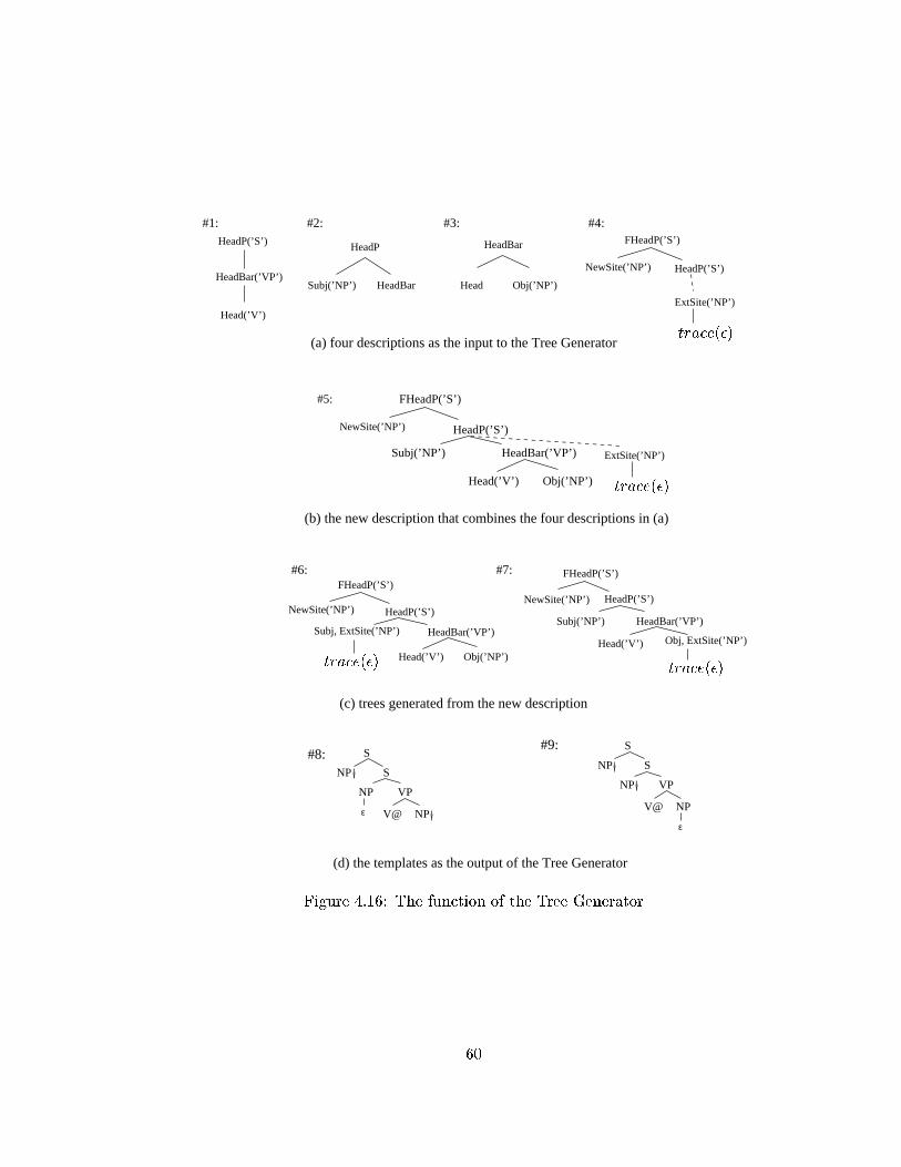
HeadP(’S’)
HeadBar(’VP’)
Head(’V’)
S
NP S
NP VP
V@ NPε
HeadBar
Head Obj(’NP’)
FHeadP(’S’)
HeadP(’S’)
Subj(’NP’) HeadBar
HeadP
#2: #3: #4:#1:
(b) the new description that combines the four descriptions in (a)
(a) four descriptions as the input to the Tree Generator
NewSite(’NP’)
#6: #7:FHeadP(’S’)
NewSite(’NP’) HeadP(’S’)
HeadBar(’VP’)
Head(’V’) Obj(’NP’)
S
NP S
NP VP
V@ NP
ε
#8:#9:
Subj, ExtSite(’NP’)
#5: FHeadP(’S’)
HeadP(’S’)
Subj(’NP’) HeadBar(’VP’)
Head(’V’) Obj(’NP’)
NewSite(’NP’)
ExtSite(’NP’)
NewSite(’NP’)
FHeadP(’S’)
HeadP(’S’)
Subj(’NP’)
Head(’V’) Obj, ExtSite(’NP’)
HeadBar(’VP’)
(c) trees generated from the new description
(d) the templates as the output of the Tree Generator
ExtSite(’NP’)
trace(�)
trace(�)trace(�)
trace(�)
Figure 4.16: The function of the Tree Generator
60
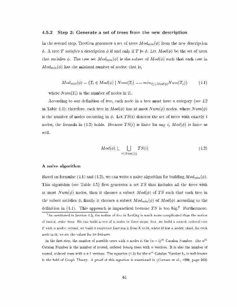
4.5.2 Step 2: Generate a set of trees from the new description
In the second step, TreeGen generates a set of trees Modmin(�) from the new description
�. A tree T satis�es a description � if and only if T j= �. Let Mod(�) be the set of trees
that satis�es �. The tree set Modmin(�) is the subset of Mod(�) such that each tree in
Modmin(�) has the minimal number of nodes; that is,
Modmin(�) = fTi 2Mod(�) j Num(Ti) ==minTj2Mod(�)Num(Tj)g (4.1)
where Num(Ti) is the number of nodes in Ti.
According to our de�nition of tree, each node in a tree must have a category (see L2
in Table 4.4); therefore, each tree in Mod(�) has at most Num(�) nodes, where Num(�)
is the number of nodes occurring in �. Let TS(i) denotes the set of trees with exactly i
nodes, the formula in (4.2) holds. Because TS(i) is �nite for any i, Mod(�) is �nite as
well.
Mod(�) �[
i�Num(�)
TS(i) (4.2)
A naive algorithm
Based on formulae (4.1) and (4.2), we can write a naive algorithm for buildingModmin(�).
This algorithm (see Table 4.5) �rst generates a set TS that includes all the trees with
at most Num(�) nodes, then it chooses a subset Mod(�) of TS such that each tree in
the subset satis�es �, �nally it chooses a subset Modmin(�) of Mod(�) according to the
de�nition in (4.1). This approach is impractical because TS is too big.8 Furthermore,
8As mentioned in Section 4.3, the notion of tree in LexOrg is much more complicated than the notion
of rooted, order trees. We can build a tree of n nodes in three steps: �rst, we build a rooted, ordered tree
T with n nodes; second, we build a surjective function I from K to U , where U has n nodes; third, for each
node in U , we set the values for its features.In the �rst step, the number of possible trees with n nodes is the (n � 1)th Catalan Number. The nth
Catalan Number is the number of rooted, ordered binary trees with n vertices. It is also the number of
rooted, ordered trees with n+1 vertices. The equation (4.3) for the nth Catalan Number bn is well-known
in the �eld of Graph Theory. A proof of this equation is mentioned in (Cormen et al., 1990, page 262)
61
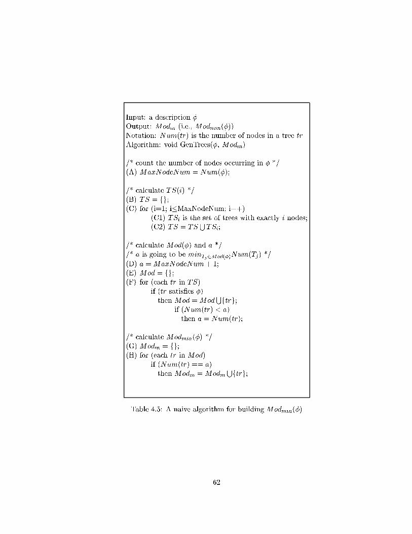
Input: a description �Output: Modm (i.e., Modmin(�))Notation: Num(tr) is the number of nodes in a tree trAlgorithm: void GenTrees(�, Modm)
/* count the number of nodes occurring in � */(A) MaxNodeNum = Num(�);
/* calculate TS(i) */(B) TS = fg;(C) for (i=1; i�MaxNodeNum; i++)
(C1) TSi is the set of trees with exactly i nodes;(C2) TS = TS
STSi;
/* calculate Mod(�) and a *//* a is going to be minTj2Mod(�)Num(Tj) */
(D) a =MaxNodeNum+ 1;(E) Mod = fg;(F) for (each tr in TS)
if (tr satis�es �)then Mod =Mod
Sftrg;if (Num(tr) < a)then a = Num(tr);
/* calculate Modmin(�) */(G) Modm = fg;(H) for (each tr in Mod)
if (Num(tr) == a)then Modm =Modm
Sftrg;
Table 4.5: A naive algorithm for buildingModmin(�)
62

the majority of trees in TS are not in Mod(�), let alone in Modmin(�); these trees are
produced in Line (C1) and then thrown away in Lines (F) and (H). A revised version of
the algorithm is shown in Table 4.6, but it still needs to calculate TS(i).
Input: a description �Output: Modm (i.e., Modmin(�))Algorithm: void GenTreesRevised(�, Modm)
/* count the number of nodes occurring in � */(A) MaxNodeNum = Num(�);
/* calculate TS(i) and Modm */(B) Modm = fg;(C) for (i=1; i�MaxNodeNum; i++)
(C1) TSi is the set of trees with exactly i nodes;(C2) for (each tr in TSi)
if (tr satis�es �)then Modm =Modm
Sftrg;(C3) if (Modm is not empty)
break;
Table 4.6: A revised version of the naive algorithm for buildingModmin(�)
A more eÆcient algorithm
The problem of the naive algorithm is that the algorithm calculates the set TS(i) without
considering �; as a result, most trees in TS(i) do not satisfy � and have to be thrown away
in later steps.
among others.
bn =1
n+ 1�
2n
n
!=
4np� � n3=2
� (1 +O(1=n)): (4.3)
In the second step, the number of possible surjective functions from K to U is S(j K j; n) � n!, whereS(m;n) is a Stirling number of the second kind; that is, S(m;n) is the number of ways that a set with m
distinguishable elements can be partitioned into n pair-wise disjoint, non-empty subsets.
Therefore, even if we don't consider feature structures, the number of trees with n nodes | the size of
TS(n) | is S(j K j; n)� n!� bn�1, which is a huge number.
63
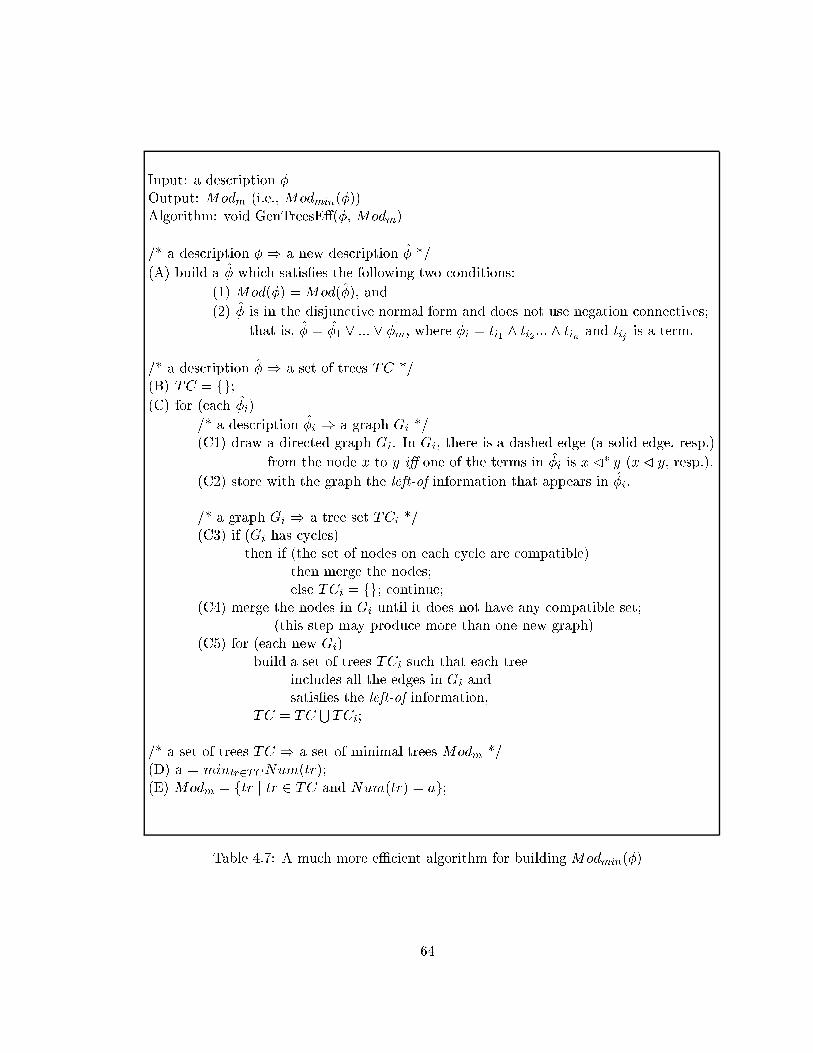
Input: a description �Output: Modm (i.e., Modmin(�))Algorithm: void GenTreesE�(�, Modm)
/* a description � ) a new description � */
(A) build a � which satis�es the following two conditions:
(1) Mod(�) =Mod(�), and
(2) � is in the disjunctive normal form and does not use negation connectives;
that is, � = �1 _ ::: _ �m, where �i = ti1 ^ ti2 ::: ^ tin and tij is a term.
/* a description � ) a set of trees TC */(B) TC = fg;(C) for (each �i)
/* a description �i ) a graph Gi */(C1) draw a directed graph Gi. In Gi, there is a dashed edge (a solid edge, resp.)
from the node x to y i� one of the terms in �i is x�� y (x� y, resp.).
(C2) store with the graph the left-of information that appears in �i.
/* a graph Gi ) a tree set TCi */(C3) if (Gi has cycles)
then if (the set of nodes on each cycle are compatible)then merge the nodes;else TCi = fg; continue;
(C4) merge the nodes in Gi until it does not have any compatible set;(this step may produce more than one new graph)
(C5) for (each new Gi)build a set of trees TCi such that each tree
includes all the edges in Gi andsatis�es the left-of information,
TC = TCSTCi;
/* a set of trees TC ) a set of minimal trees Modm */(D) a = mintr2TCNum(tr);(E) Modm = ftr j tr 2 TC and Num(tr) = ag;
Table 4.7: A much more eÆcient algorithm for building Modmin(�)
64

B(’b’)
A(’a’)
D(’d’)
C,E(’c’)
F(’b’)
G(’b’)B(’b’) C(’c’)
A(’a’)
D(’d’) E
F(’b’)
G(’b’)
B(’b’)
A(’a’)
D(’d’)
C,E(’c’)
F,G(’b’)
A(’a’)
D(’d’)
B,G(’b’) C,E(’c’)
F(’b’)
(e) the trees built from the graphs
(d) the graphs after compatible sets are merged
(c) the graph after cycles are removed(b) a graph built from the description
(a) a description
A(’a’)
D(’d’)
C,E(’c’)B,G(’b’)
F(’b’)
B(’b’)
A(’a’)
D(’d’)
C,E(’c’)
F,G(’b’)
#3:
#1:
#2:
#4: #5:
#7:#6:
(A�� B) ^ (A�� C) ^ (C �D) ^ (C �� E)^(E �� C) ^ (E � F ) ^ (G�H) ^ (B � E)^(A:label =0 a0) ^ (B:label =0 b0) ^ (C:label =0 c0) ^ (D:label =0 d0)(F:label =0 b0) ^ (G:label =0 b0) ^ (H:label =0 �0)
Left-of information: B � E
Left-of information: B � C;E
Left-of information: B � C;E
Left-of information: B;G � C;E
H(�)
H(�)
H(�)
H(�)
H(�)
H(�)
Figure 4.17: An example that illustrates how the new algorithm works
65

We propose an algorithm that is much more eÆcient. The main idea is as follows.
First, we build a new description � such that a tree satis�es � if and only it satis�es �, and
� is in disjunctive normal form and it does not use negative connectives. Second, for each
branch �i in �, we build a graph Gi. A graph is a model for LK as de�ned in Table 4.4,
but it is not necessarily a tree. Third, we turn each Gi into a tree. There may be more
than one possible tree; as a result, we get a set of trees TCi. Last, we choose the subset
ofSTCi with the minimal number of nodes.
The new algorithm is in Table 4.7. Figure 4.17 shows a description and the output
after each major step. Some explanations about the algorithm are in order.
� Line (A): The algorithm builds � from � in line (A) in order to create a graph for
each component �i of �. � is not necessarily equivalent to �. In �rst-order logic,
two formulae are equivalent if any model that satis�es one formula also satis�es the
other formula and vice versa. The condition (1) in Table 4.7 requires that the sets of
trees (not models) that satisfy � and � are identical. � is built in three steps. First,
the algorithm builds a formula �0 which is equivalent to � and is in the disjunctive
normal form. In �0, negation connectives negate only terms, rather than formulae.
Second, if �0 includes negations of terms, the algorithm builds a new description �00
by replacing negations of terms with disjunctions of terms without negations. For
instance, it replaces :(a � b) with (a �� b) _ (b �� a) _ (b � a). This replacement
is possible because any tree | including the ones in Mod(�) | has to satisfy the
conditions in Tables 4.2 and 4.4. The resulting formula �00 does not include any
negative connective. Last, we build a formula � in the disjunctive normal form
which is equivalent to �00, and � does not include negative connectives.
� Lines (C3) and (C4): the process in Line (C1) can be easily reversed to build a
description �(G) from a graph G. We call a graph G consistent if there is at least
one tree that satis�es �(G). We call a set of nodes in a graph compatible if after
merging them into a single node, the resulting graph is still consistent. When nodes
are merged, the left-of information and dashed/solid edges in the graph have to be
updated accordingly, as shown in Figure 4.17(c){(d).
66
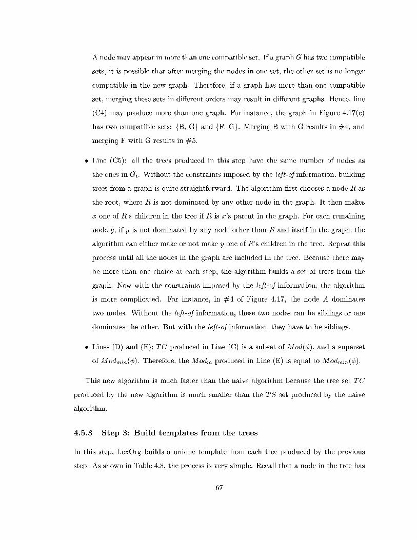
A node may appear in more than one compatible set. If a graphG has two compatible
sets, it is possible that after merging the nodes in one set, the other set is no longer
compatible in the new graph. Therefore, if a graph has more than one compatible
set, merging these sets in di�erent orders may result in di�erent graphs. Hence, line
(C4) may produce more than one graph. For instance, the graph in Figure 4.17(c)
has two compatible sets: fB, Gg and fF, Gg. Merging B with G results in #4, and
merging F with G results in #5.
� Line (C5): all the trees produced in this step have the same number of nodes as
the ones in Gi. Without the constraints imposed by the left-of information, building
trees from a graph is quite straightforward. The algorithm �rst chooses a node R as
the root, where R is not dominated by any other node in the graph. It then makes
x one of R's children in the tree if R is x's parent in the graph. For each remaining
node y, if y is not dominated by any node other than R and itself in the graph, the
algorithm can either make or not make y one of R's children in the tree. Repeat this
process until all the nodes in the graph are included in the tree. Because there may
be more than one choice at each step, the algorithm builds a set of trees from the
graph. Now with the constraints imposed by the left-of information, the algorithm
is more complicated. For instance, in #4 of Figure 4.17, the node A dominates
two nodes. Without the left-of information, these two nodes can be siblings or one
dominates the other. But with the left-of information, they have to be siblings.
� Lines (D) and (E): TC produced in Line (C) is a subset of Mod(�), and a superset
of Modmin(�). Therefore, the Modm produced in Line (E) is equal to Modmin(�).
This new algorithm is much faster than the naive algorithm because the tree set TC
produced by the new algorithm is much smaller than the TS set produced by the naive
algorithm.
4.5.3 Step 3: Build templates from the trees
In this step, LexOrg builds a unique template from each tree produced by the previous
step. As shown in Table 4.8, the process is very simple. Recall that a node in the tree has
67

Subj(’NP’) HeadBar(’VP’)
Head(’V’) Obj,ExtSite(’NP’)
HeadP(’S’)NewSite(’NP’)
FHeadP(’S’)
(a) a tree (b) the corresponding template
S
NP S
NP VP
NPV@
Trace(0�0)�
Figure 4.18: A tree and the template built from it
the form fkig(ffm = vng). LexOrg replaces fkig(ffm = vng) with l(ffm = vng), where l isthe category of ki. If the type of a leaf node is unspeci�ed, LexOrg sets the type according
to the defaults given in line (A2) in Table 4.8. Figure 4.11 (repeated as Figure 4.18) shows
a tree and the template built from the tree.
4.6 The Description Selector
In this section, we introduce a second component of LexOrg named Description Selector,
which takes as input a subcategorization frame Fr and a set of description DescSet, and
outputs subsets of DescSet.
4.6.1 The function of the Description Selector
In the previous section, we showed that the Tree Generator builds elementary trees from
a set of descriptions, as illustrated in Figure 4.16. A simpli�ed version of the �gure is
repeated as Figure 4.19. The set of descriptions given to the Tree Generator is a subset
of the descriptions provided by the users. The function of the Description Selector is to
select the descriptions for the Tree Generator; that is, it takes as input a subcategorization
frame and a �nite set of descriptions, and produces sets of descriptions, which are then fed
to the Tree Generator. An example is given in Figure 4.20. In this example, the inputs
to the Description Selector are a set DescSet of descriptions (i.e., fD1, D2, D3, D4, D5g)and a subcategorization frame Fr; the output is a set with four members: SD1, SD2,
SD3, and SD4. Each SDi is a subset of DescSet. The Tree Generator takes each SDi and
68

Input: a tree TrOutput: a template TempAlgorithm: void GenTemp(Tr, Temp)(A) for (each node n in Tr)
(A1) Let n be of the form \fkig(cat = a; type = b; subsc = c; f1 = v1; :::; fn = vn)",create a new node n0 of the form \a(f1 = v1; :::; fn = vn)";
(A2) if (n is a leaf node)if (n:type is unspeci�ed)then if (one of the symbols in fkig is Head)
then mark n0 as an anchor node;else if (one of the symbols in fkig is ModFoot)
then mark n0 as a foot node;else mark n0 as a substitution node;
else mark n0 according to the value of n:type;
(A3) if (n:subsc is de�ned)then set the subscript of n0 to be n:subsc;
(B) for (each edge from n1 to n2 in Tr)add an edge from n01 to n
02 in Temp
Table 4.8: An algorithm that builds a template from a tree
69
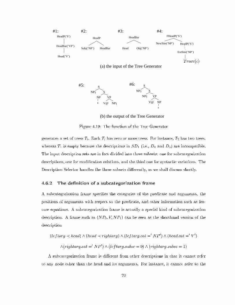
HeadP(’S’)
HeadBar(’VP’)
Head(’V’)
S
NP S
NP VP
V@ NPε
S
NP S
NP VP
V@ NP
ε
HeadBar
Head Obj(’NP’)
FHeadP(’S’)
HeadP(’S’)
Subj(’NP’) HeadBar
HeadP
NewSite(’NP’)
ExtSite(’NP’)
(a) the input of the Tree Generator
#5: #6:
#1: #2: #3: #4:
(b) the output of the Tree Generator
Trace(�)
Figure 4.19: The function of the Tree Generator
generates a set of trees Ti. Each Ti has zero or more trees. For instance, T2 has two trees,
whereas T4 is empty because the descriptions in SD4 (i.e., D4 and D5) are incompatible.
The input description sets are in fact divided into three subsets: one for subcategorization
descriptions, one for modi�cation relations, and the third one for syntactic variations. The
Description Selector handles the three subsets di�erently, as we shall discuss shortly.
4.6.2 The de�nition of a subcategorization frame
A subcategorization frame speci�es the categories of the predicate and arguments, the
positions of arguments with respect to the predicate, and other information such as fea-
ture equations. A subcategorization frame is actually a special kind of subcategorization
description. A frame such as (NP0; V;NP1) can be seen as the shorthand version of the
description
(leftarg � head) ^ (head � rightarg) ^ (leftarg:cat =0 NP 0) ^ (head:cat =0 V 0)
^(rightarg:cat =0 NP 0) ^ (leftarg:subsc = 0) ^ (rightarg:subsc = 1)
A subcategorization frame is di�erent from other descriptions in that it cannot refer
to any node other than the head and its arguments. For instance, it cannot refer to the
70

HeadP(’S’)
HeadBar(’VP’)
Head(’V’)
Subj(’NP’) HeadBar
HeadP HeadBar
Head Obj(’NP’)
S
V@ NP
VPNP
ε1
0
S
NP
S
NP SNP VP
NPV@
ε
1
0
VP*
VP
S
V@ NP
VPNP
ε1
0
S
NP VP
V@ NP1
0
S
NP VP
V@ NP1
0
VP*
VP
S
V@ NP
VPNP
ε1
0
S
V@ NP
VPNP
ε1
0
S
NP
S
NP SNP VP
NPV@
ε
1
0
Tree Generator
Description Selector
FHeadP(’S’)
HeadP(’S’)NewSite(’NP’)
ExtSite(’NP’)
ModRoot(’VP’)
ModFoot(’VP’) HeadP(’S’)
Subj(’NP’)
tree family for the transitive verb
the union of the sets T
(D )
(T ) 41 2(T ) (T ) (T )
3
(SD )(SD )(SD )1 2 3
(D ) (D ) (D ) (D )1 2 3 54
(NP0, V, NP1)
D3, D4, D5Fr, D1, D2,
(SD )4
Fr:
Fr, D1, D2, D3 Fr, D1, D2,D3, D4
Fr, D1, D2, D3, D5
i
Trace(�) PRO(�)
Figure 4.20: The function of the Description Selector
71

VP which is the parent of the verb head. Another di�erence is that the categories of the
nodes in a subcategorization frame must be speci�ed.
4.6.3 The algorithm for the Description Selector
Now that we have described the function of the Description Selector, the next question is
how does it work? In Section 4.4, we classify descriptions into four types: the ones for head
projections, head-argument relations, syntactic variations, and modi�cation relations. The
�rst two types (e.g., D1;D2 andD3 in Figure 4.20) are also called subcategorization descrip-
tions since they specify structures for a particular subcategorization frame. Because the
elementary trees in a tree family have the same subcategorization frame, the Description
Selector should put in every SDi all the subcategorization descriptions for that subcate-
gorization frame. In addition to subcategorization information, an elementary tree may
include information about zero or more syntactic variations, and zero or one modi�cation
relation. Therefore, each SDi built by the Description Selector should include all the
related subcategorization descriptions, zero or more syntactic variation descriptions, and
zero or one modi�cation description.
The algorithm for the Description Selector is in Table 4.9. Some explanations are in
order.
� In Line (A), the algorithm chooses a subset of subcategorization descriptions by
matching the \headers" of descriptions with the \headers" that are automatically
generated from a subcategorization frame. To see how it works, just imagine that
each description is a function with a header and a body. The header is made
of a function name and a list of parameters in particular formats. The body is
a w� as de�ned before. For instance, the headers of the descriptions in D1 |
D3 in Figure 4.20 are head is V (Head), head V has left arg NP (Head, Subj), and
head V has right arg NP (Head, Obj), respectively. Given a subcategorization frame
(L1; L2; :::; Ln;X;R1; R2; :::; Rm), the algorithm generates a set of headers such as
head is X (Head), head X has a left arg Li (Head, LArgi), and head X has a right arg Ri
(Head, RArgi). Then it uses this set of headers to fetch the descriptions with the
72
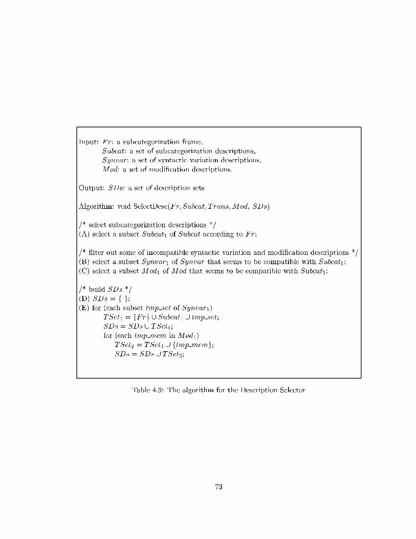
Input: Fr: a subcategorization frame,Subcat: a set of subcategorization descriptions,Synvar: a set of syntactic variation descriptions,Mod: a set of modi�cation descriptions.
Output: SDs: a set of description sets
Algorithm: void SelectDesc(Fr; Subcat; T rans;Mod, SDs)
/* select subcategorization descriptions */(A) select a subset Subcat1 of Subcat according to Fr;
/* �lter out some of incompatible syntactic variation and modi�cation descriptions */(B) select a subset Synvar1 of Synvar that seems to be compatible with Subcat1;(C) select a subset Mod1 of Mod that seems to be compatible with Subcat1;
/* build SDs */(D) SDs = f g;(E) for (each subset tmp set of Synvar1)
TSet1 = fFrg [ Subcat1 [ tmp set;SDs = SDs [ TSet1;for (each tmp mem in Mod1)
TSet2 = TSet1 [ ftmp memg;SDs = SDs [ TSet2;
Table 4.9: The algorithm for the Description Selector
73
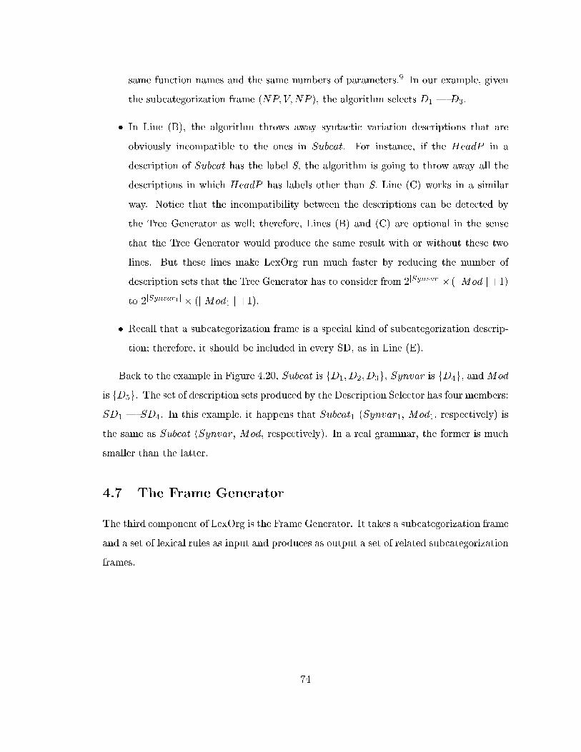
same function names and the same numbers of parameters.9 In our example, given
the subcategorization frame (NP; V;NP ), the algorithm selects D1 | D3.
� In Line (B), the algorithm throws away syntactic variation descriptions that are
obviously incompatible to the ones in Subcat. For instance, if the HeadP in a
description of Subcat has the label S, the algorithm is going to throw away all the
descriptions in which HeadP has labels other than S. Line (C) works in a similar
way. Notice that the incompatibility between the descriptions can be detected by
the Tree Generator as well; therefore, Lines (B) and (C) are optional in the sense
that the Tree Generator would produce the same result with or without these two
lines. But these lines make LexOrg run much faster by reducing the number of
description sets that the Tree Generator has to consider from 2jSynvarj�(jMod j +1)to 2jSynvar1j � (jMod1 j +1).
� Recall that a subcategorization frame is a special kind of subcategorization descrip-
tion; therefore, it should be included in every SD, as in Line (E).
Back to the example in Figure 4.20, Subcat is fD1;D2;D3g, Synvar is fD4g, andMod
is fD5g. The set of description sets produced by the Description Selector has four members:SD1 | SD4. In this example, it happens that Subcat1 (Synvar1, Mod1, respectively) is
the same as Subcat (Synvar, Mod, respectively). In a real grammar, the former is much
smaller than the latter.
4.7 The Frame Generator
The third component of LexOrg is the Frame Generator. It takes a subcategorization frame
and a set of lexical rules as input and produces as output a set of related subcategorization
frames.
74
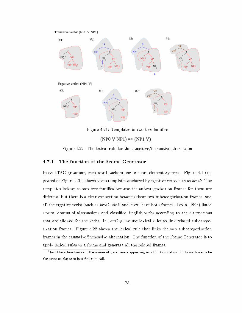
0
NP
VP
1
NPNP
NP
S
ε
VP
NP
0
V@
#2:
S NP S
V@1
NP1
0
V@
ε
#3:
S
S
VP1
V@
NP VP
S
NP
Transitive verbs: (NP0 V NP1)
#1: #4:
Ergative verbs: (NP1 V)
NP
S
ε
S
NP VP
VP
VP* S
VP
ε
NP
1
V@
1
V@
#5: #7:#6:
VP
VP* S
0 VP
NPε
NP
1V@
Figure 4.21: Templates in two tree families
(NP0 V NP1) => (NP1 V)
Figure 4.22: The lexical rule for the causative/inchoative alternation
4.7.1 The function of the Frame Generator
In an LTAG grammar, each word anchors one or more elementary trees. Figure 4.1 (re-
peated as Figure 4.21) shows seven templates anchored by ergative verbs such as break. The
templates belong to two tree families because the subcategorization frames for them are
di�erent, but there is a clear connection between these two subcategorization frames, and
all the ergative verbs (such as break, sink, and melt) have both frames. Levin (1993) listed
several dozens of alternations and classi�ed English verbs according to the alternations
that are allowed for the verbs. In LexOrg, we use lexical rules to link related subcatego-
rization frames. Figure 4.22 shows the lexical rule that links the two subcategorization
frames in the causative/inchoative alternation. The function of the Frame Generator is to
apply lexical rules to a frame and generate all the related frames.
9Just like a function call, the names of parameters appearing in a function de�nition do not have to be
the same as the ones in a function call.
75

4.7.2 The de�nition of a lexical rule
The term lexical rule is heavily overloaded. For instance, the lexical rules in (Evans et al.,
1995) can manipulate tree structures. They are used to account for wh-movement, topical-
ization, and so on. In LexOrg, lexical rules can only manipulate subcategorization frames.
A lexical rule is of the form fr1 ) fr2, where fr1 and fr2 are just like subcategorization
frames except that the categories of the nodes in fr1 and fr2 do not have to be speci�ed.
A lexical rule fr1 ) fr2 is said to be applicable to a frame fr if fr and fr1 are
compatible; that is, fr and fr1 have the same number of arguments and the features of
the corresponding nodes can be uni�ed. Applying this rule to fr yields a new frame which
combines the information in fr and fr2. For instance, the lexical rule (Subj; V; S) )(Subj; V;NP ) says that if a verb can take an S object, it can also take an NP object.
Applying this rule to the frame (NP0 V S1) generates a new frame (NP0 V NP). In this
new frame, the category of the subject comes from the input frame, where the category
of the object comes from the right frame of the lexical rule. Because the category of the
Subj in the lexical rule is not speci�ed, the lexical rule is also applicable to the frame (S0
V S1).
In addition to categories, the nodes in a lexical rule may include other features. For
instance, a lexical rule for passivization would look exactly like the one in Figure 4.22
except that the feature voice has the value 'active' for the verb in the left frame, and has
the value 'passive' for the same verb in the right frame. This feature will prevent the rule
from being applied to a verb that is already in the passive voice, such as given in John is
given a book.
4.7.3 The algorithm for the Frame Generator
The Frame Generator takes a subcategorization frame Fr and a set of lexical rules Rules
as input and produces as output a set of related frames. Initially, Fr is the only member
of FrSet . Then the Frame Generator applies each rule in Rules to each frame in FrSet,
and adds the resulting frames to FrSet. It repeats this step until no more new frames are
added to FrSet.
In this process, the Frame Generator may apply a rule r1 to a frame f1 and generate a
76
frame f2, and then apply r2 to f2 and generate f3, and so on. When that happens, we say
that a sequence [r1; r2; :::; rn] of lexical rules is applied to the frame f1 . The order of the
lexical rules in the sequence is important. For example, a passivization rule is applicable
after the dative shift rule is applied to the subcategorization frame for ditransitive verbs,
but the dative shift rule is not applicable after a passivization rule is applied to the same
frame. Also, the set of possible sequences of lexical rules is �nite because the set of distinct
lexical rules is �nite and in general each lexical rule appears in a sequence at most once.10
Therefore, this three-step process will eventually terminate.
Lexical rules and syntactic variation descriptions are very di�erent in several aspects.
First, a lexical rule is a function that takes a subcategorization frame as input, and produces
another frame as output; a syntactic variation description is a w� in a simpli�ed �rst-order
logic. Second, lexical rules are more idiosyncratic than syntactic variations. For instance,
the lexical rule in Figure 4.22 is only applicable to ergative verbs, rather than all the
transitive verbs. In contrast, the description for wh-movement applies to all the verbs.
Third, when lexical rules are applied to a subcategorization frame in a series, the order
of the lexical rules matters. In contrast, if a set of descriptions includes more than one
syntactic variation description (e.g., the descriptions for topicalization and argument drop
in Chinese), the order between the descriptions does not matter. Last, lexical rules can be
non-additive, allowing arguments to be removed; descriptions are strictly additive, meaning
a description can only add information, not remove information.
4.8 The experiments
In previous sections, we have described three components of LexOrg, which can be sum-
marized as follows:
� The goal of LexOrg is to provide an eÆcient way to generate templates for a language.
As shown in Figure 4.4 (repeated here as Figure 4.23), the inputs to LexOrg are a
10An arguable exception to this claim is the double causative construction in languages such as Hungarian
(Shibatani, 1976). But in this construction it is not clear whether the second causativization is done in
morphology or in syntax. Even if it is done at the morphological level, the two causativizations are not
exactly the same and they will be represented as two di�erent lexical rules in LexOrg.
77
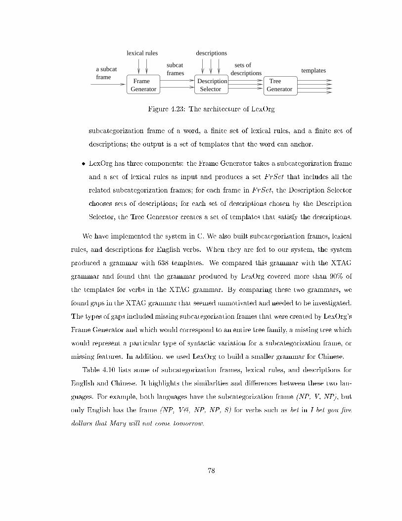
GeneratorFrame Description
Selector
framedescriptions
sets of
GeneratorTree
templates
descriptions
a subcatframessubcat
lexical rules
Figure 4.23: The architecture of LexOrg
subcategorization frame of a word, a �nite set of lexical rules, and a �nite set of
descriptions; the output is a set of templates that the word can anchor.
� LexOrg has three components: the Frame Generator takes a subcategorization frame
and a set of lexical rules as input and produces a set FrSet that includes all the
related subcategorization frames; for each frame in FrSet, the Description Selector
chooses sets of descriptions; for each set of descriptions chosen by the Description
Selector, the Tree Generator creates a set of templates that satisfy the descriptions.
We have implemented the system in C. We also built subcategorization frames, lexical
rules, and descriptions for English verbs. When they are fed to our system, the system
produced a grammar with 638 templates. We compared this grammar with the XTAG
grammar and found that the grammar produced by LexOrg covered more than 90% of
the templates for verbs in the XTAG grammar. By comparing these two grammars, we
found gaps in the XTAG grammar that seemed unmotivated and needed to be investigated.
The types of gaps included missing subcategorization frames that were created by LexOrg's
Frame Generator and which would correspond to an entire tree family, a missing tree which
would represent a particular type of syntactic variation for a subcategorization frame, or
missing features. In addition, we used LexOrg to build a smaller grammar for Chinese.
Table 4.10 lists some of subcategorization frames, lexical rules, and descriptions for
English and Chinese. It highlights the similarities and di�erences between these two lan-
guages. For example, both languages have the subcategorization frame (NP, V, NP), but
only English has the frame (NP, V@, NP, NP, S) for verbs such as bet in I bet you �ve
dollars that Mary will not come tomorrow.
78

English Chinese
subcategorization (NP, V, NP) (NP, V, NP)frames (NP, V, NP, NP, S) (V)
lexical passive short bei-construles dative-shift V-de construction
subcategorization head is V head is Vdescriptions V has 3 right arg V has 2 right arg
syntactic variation wh-question topicalizationdescriptions imperative argument drop
modi�cation S modify VP from right S modify VP from rightdescriptions S modify NP from right S modify NP from left
Table 4.10: Some examples of subcategorization frames, lexical rules, and descriptions forEnglish and Chinese
4.9 Creating language-speci�c information
LexOrg generates templates from subcategorization frames, lexical rules, and descriptions.
It presumes that users of LexOrg provide this information to the system. A natural
question arises: how does a user create such information? We address this question in this
section.
4.9.1 Subcategorization frames and lexical rules
Only a limited number of categories (such as verbs and prepositions) take arguments and
therefore have nontrivial subcategorization frames and lexical rules. By nontrivial, we
mean subcategorization frames with at least one argument. Among these categories, verbs
are the most complicated ones. To create subcategorization frames and lexical rules for
verbs, the user of LexOrg can refer to the literature on verb classes such as (Levin, 1993).
In this book, Levin discussed verb classes and alternations for verbs. Many alternations in
her book are represented as lexical rules in LexOrg. In the next chapter, we shall discuss
another system (LexTract) which can extract subcategorization frames from bracketed
corpora.
79
4.9.2 Descriptions
In addition to subcategorization frames and lexical rules, the users of LexOrg need to
build descriptions. They can choose one or more of the following three approaches to build
descriptions.
From templates
In the �rst approach, users start with some templates that they want LexOrg to build and
see how they can decompose the templates into sets of descriptions. For instance, given a
template in Figure 4.24(a), we know that it is for a predicate-argument relation, and there-
fore the set of descriptions should include zero modi�cation descriptions, a head projection
description, several head-argument descriptions, and one or more syntactic variation de-
scriptions. One thing that is not clear from the template alone is whether the root S node
in the template is a lexical projection or a functional projection of the anchor V. If it is a
lexical projection, the verb has three NP arguments: two appears before the verb, and one
appears after the verb and it is dropped (recall that arguments can be dropped in Chinese
and Korean). In this case, the description set in Figure 4.24(b) should be used. In this
set, #1 is for the head and its projection, #2, #3, and #4 are for arguments of the head,
#5 is for a syntactic variation such as argument-drop. If the root S node is a functional
projection, the verb has two NP arguments: one appears before the verb, and the other is
generated after the verb but it is later moved to the sentence-initial position (e.g., it may
undergo wh-movement). In this case, the description set in Figure 4.25 should be used,
where #1 is for the head and its projection, #2 and #3 are for arguments, and #4 is for
a syntactic variation such as wh-movement. Although the template alone does not pro-
vide suÆcient information to make the decomposition unique, with the knowledge about
a language (e.g., the verb's projection levels and the existence of overt wh-movement and
argument-drop in the language), the users should be able to choose the correct description
set.
In Section 4.4, we classi�ed descriptions according to four types of information (i.e.,
head and it projections, arguments of a head, modi�ers of a head, and syntactic variations)
expressed in the descriptions. This classi�cation greatly reduces the number of possible
80

S
NP S
NP VP
V NP
ε
Y1(’NP’) X1(’S’)
X0(’S’)
Y3(’NP’)
X2
Head
Y2(’NP’)
X1
X2
(a) a template
#1:#2:
#3:
(b) a set of descriptions
#4:
#5:Y3(’NP’)
εZ1(’ ’)
X1(’S’)
X2(’VP’)
Head(’V’)
X0(’S’)
Figure 4.24: A template and a set of descriptions that can generate it
HeadP(’S’)
HeadBar(’VP’)
Head(’V’)
HeadBar
Head Obj(’NP’)
FHeadP(’S’)
HeadP(’S’)
Subj(’NP’) HeadBar
HeadP
#2: #3: #4:#1:
NewSite(’NP’)
ExtSite(’NP’)
trace(�)
Figure 4.25: A more desirable description set if the template is for English
81
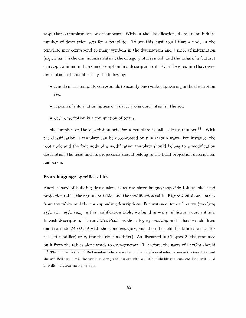
ways that a template can be decomposed. Without the classi�cation, there are an in�nite
number of description sets for a template. To see this, just recall that a node in the
template may correspond to many symbols in the descriptions and a piece of information
(e.g., a pair in the dominance relation, the category of a symbol, and the value of a feature)
can appear in more than one description in a description set. Even if we require that every
description set should satisfy the following:
� a node in the template corresponds to exactly one symbol appearing in the description
set.
� a piece of information appears in exactly one description in the set.
� each description is a conjunction of terms.
the number of the description sets for a template is still a huge number.11 With
the classi�cation, a template can be decomposed only in certain ways. For instance, the
root node and the foot node of a modi�cation template should belong to a modi�cation
description, the head and its projections should belong to the head projection description,
and so on.
From language-speci�c tables
Another way of building descriptions is to use three language-speci�c tables: the head
projection table, the argument table, and the modi�cation table. Figure 4.26 shows entries
from the tables and the corresponding descriptions. For instance, for each entry (mod tag
x1=:::=xn y1=:::=ym) in the modi�cation table, we build m+ n modi�cation descriptions.
In each description, the root ModRoot has the category mod tag and it has two children:
one is a node ModFoot with the same category, and the other child is labeled as xi (for
the left modi�er) or yi (for the right modi�er). As discussed in Chapter 3, the grammar
built from the tables alone tends to over-generate. Therefore, the users of LexOrg should
11The number is the nth Bell number, where n is the number of pieces of information in the template, and
the nth Bell number is the number of ways that a set with n distinguishable elements can be partitioned
into disjoint, non-empty subsets.
82
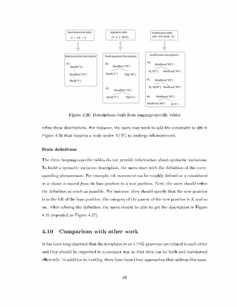
head projection table:
V -> VP -> S
argument table
(V 0 2 NP/S)
HeadBar(’VP’)
Head(’V’) Obj(’S’)
HeadBar(’VP’)
Head(’V’) Obj(’NP’)
Head(’V’)
HeadP(’S’)
HeadBar(’VP’)X(’DT’) ModFoot(’NP’)
ModRoot(’NP’)
modification descriptions:
X(’ADJP’) ModFoot(’NP’)
ModRoot(’NP’)
ModRoot(’NP’)
#4:
#5:
#6:
X(’S’)ModFoot(’NP’)
head-argument descriptions:head projection description:
#1: #2:
#3:
modification table(NP DT/ADJP S)
Figure 4.26: Descriptions built from language-speci�c tables
re�ne these descriptions. For instance, the users may want to add the constraint to #6 in
Figure 4.26 that requires a node under X('S') to undergo wh-movement.
From de�nitions
The three language-speci�c tables do not provide information about syntactic variations.
To build a syntactic variation description, the users start with the de�nition of the corre-
sponding phenomenon. For example, wh-movement can be roughly de�ned as a constituent
in a clause is moved from its base position to a new position. Next, the users should re�ne
the de�nition as much as possible. For instance, they should specify that the new position
is to the left of the base position, the category of the parent of the new position is S, and so
on. After re�ning the de�nition, the users should be able to get the description in Figure
4.15 (repeated as Figure 4.27).
4.10 Comparison with other work
It has been long observed that the templates in an LTAG grammar are related to each other
and they should be organized in a compact way so that they can be built and maintained
eÆciently. In addition to LexOrg, there have been three approaches that address this issue.
83
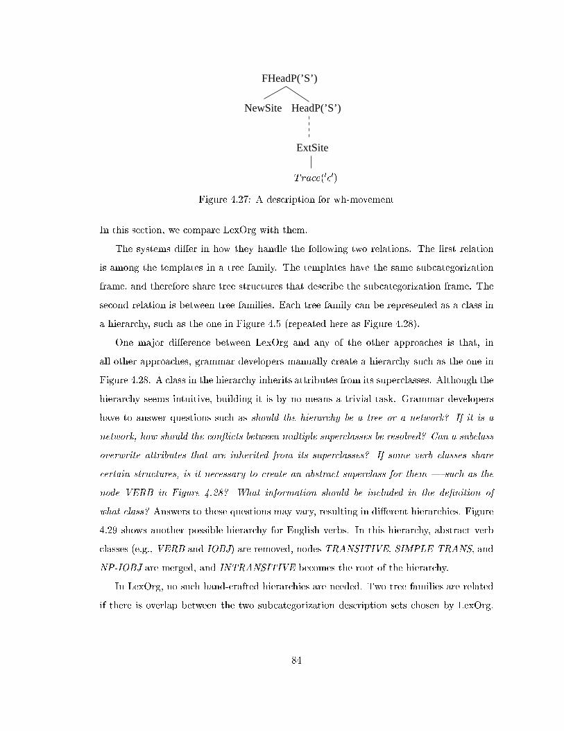
FHeadP(’S’)
HeadP(’S’)NewSite
ExtSite
Trace(0�0)
Figure 4.27: A description for wh-movement
In this section, we compare LexOrg with them.
The systems di�er in how they handle the following two relations. The �rst relation
is among the templates in a tree family. The templates have the same subcategorization
frame, and therefore share tree structures that describe the subcategorization frame. The
second relation is between tree families. Each tree family can be represented as a class in
a hierarchy, such as the one in Figure 4.5 (repeated here as Figure 4.28).
One major di�erence between LexOrg and any of the other approaches is that, in
all other approaches, grammar developers manually create a hierarchy such as the one in
Figure 4.28. A class in the hierarchy inherits attributes from its superclasses. Although the
hierarchy seems intuitive, building it is by no means a trivial task. Grammar developers
have to answer questions such as should the hierarchy be a tree or a network? If it is a
network, how should the con icts between multiple superclasses be resolved? Can a subclass
overwrite attributes that are inherited from its superclasses? If some verb classes share
certain structures, is it necessary to create an abstract superclass for them | such as the
node VERB in Figure 4.28? What information should be included in the de�nition of
what class? Answers to these questions may vary, resulting in di�erent hierarchies. Figure
4.29 shows another possible hierarchy for English verbs. In this hierarchy, abstract verb
classes (e.g., VERB and IOBJ) are removed, nodes TRANSITIVE, SIMPLE-TRANS, and
NP-IOBJ are merged, and INTRANSITIVE becomes the root of the hierarchy.
In LexOrg, no such hand-crafted hierarchies are needed. Two tree families are related
if there is overlap between the two subcategorization description sets chosen by LexOrg.
84
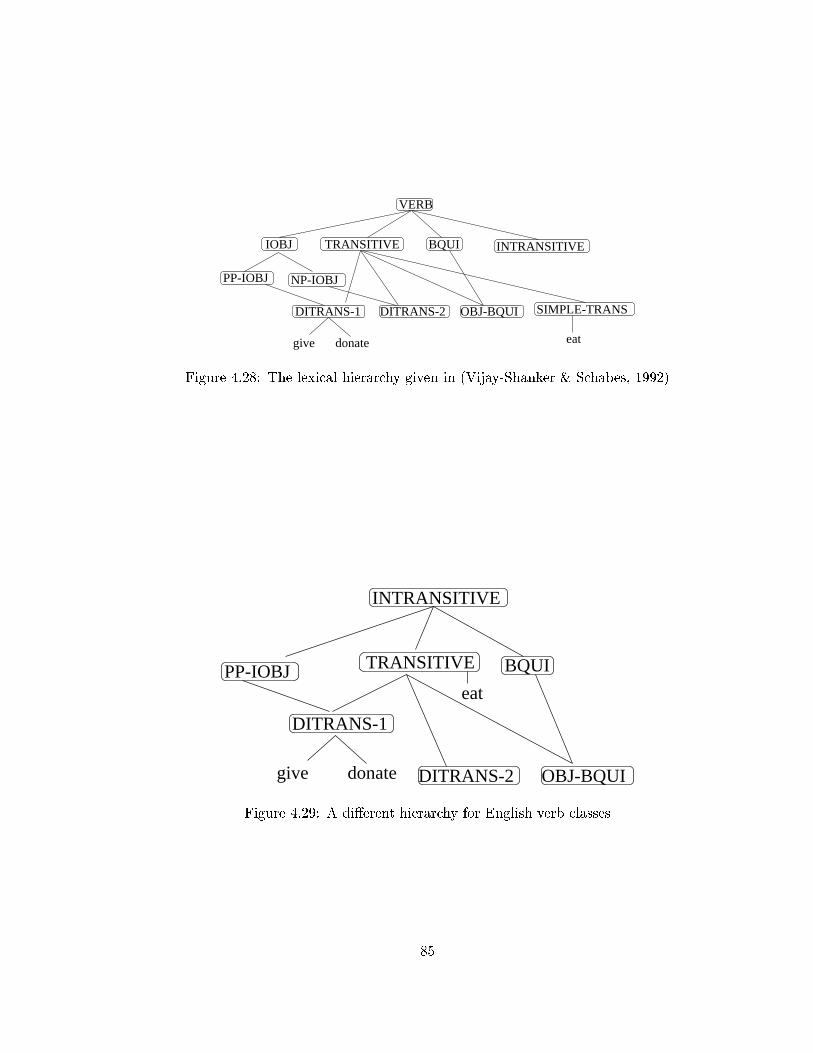
TRANSITIVE BQUI INTRANSITIVE
PP-IOBJ NP-IOBJ
DITRANS-1 DITRANS-2 OBJ-BQUI SIMPLE-TRANS
IOBJ
VERB
eatgive donate
Figure 4.28: The lexical hierarchy given in (Vijay-Shanker & Schabes, 1992)
BQUIPP-IOBJ
DITRANS-1
INTRANSITIVE
DITRANS-2 OBJ-BQUI
TRANSITIVE
give donate
eat
Figure 4.29: A di�erent hierarchy for English verb classes
85
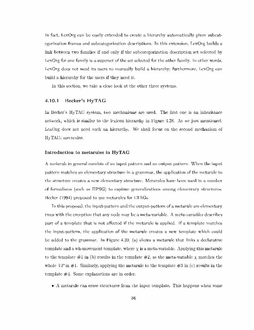
In fact, LexOrg can be easily extended to create a hierarchy automatically given subcat-
egorization frames and subcategorization descriptions. In this extension, LexOrg builds a
link between two families if and only if the subcategorization description set selected by
LexOrg for one family is a superset of the set selected for the other family. In other words,
LexOrg does not need its users to manually build a hierarchy; furthermore, LexOrg can
build a hierarchy for the users if they need it.
In this section, we take a close look at the other three systems.
4.10.1 Becker's HyTAG
In Becker's HyTAG system, two mechanisms are used. The �rst one is an inheritance
network, which is similar to the lexicon hierarchy in Figure 4.28. As we just mentioned,
LexOrg does not need such an hierarchy. We shall focus on the second mechanism of
HyTAG: metarules.
Introduction to metarules in HyTAG
A metarule in general consists of an input pattern and an output pattern. When the input
pattern matches an elementary structure in a grammar, the application of the metarule to
the structure creates a new elementary structure. Metarules have been used in a number
of formalisms (such as HPSG) to capture generalizations among elementary structures.
Becker (1994) proposed to use metarules for LTAGs.
In this proposal, the input-pattern and the output-pattern of a metarule are elementary
trees with the exception that any node may be a meta-variable. A meta-variables describes
part of a template that is not a�ected if the metarule is applied. If a template matches
the input-pattern, the application of the metarule creates a new template which could
be added to the grammar. In Figure 4.30, (a) shows a metarule that links a declarative
template and a wh-movement template, where � is a meta-variable. Applying this metarule
to the template #1 in (b) results in the template #2, as the meta-variable � matches the
whole VP in #1. Similarly, applying the metarule to the template #3 in (c) results in the
template #4. Some explanations are in order.
� A metarule can erase structures from the input template. This happens when some
86
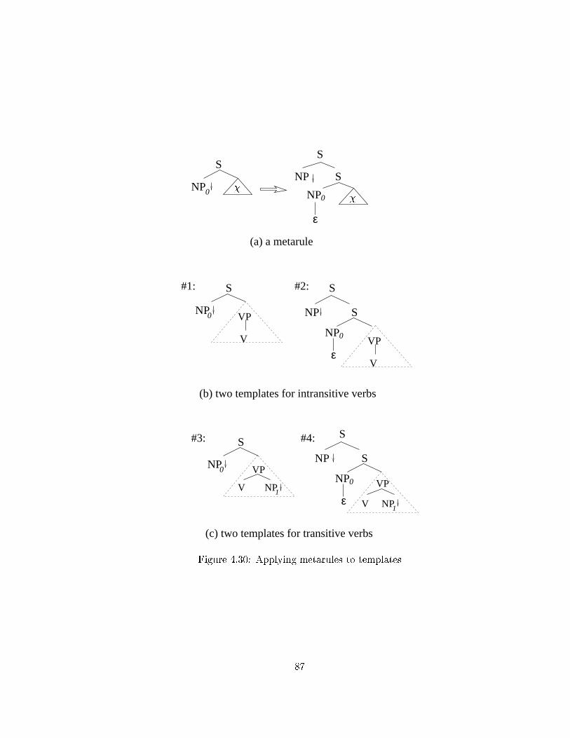
VP
V NP1
(a) a metarule
S
NP0 NP0
ε
S
S
NP
#1: #2:S
NP S
NP
S
NP
ε
0
0V
VP
VP
V
(b) two templates for intransitive verbs
#4:#3: S
NP0S
NP
S
NP
ε
0 VP
V NP1
(c) two templates for transitive verbs
��
Figure 4.30: Applying metarules to templates
87
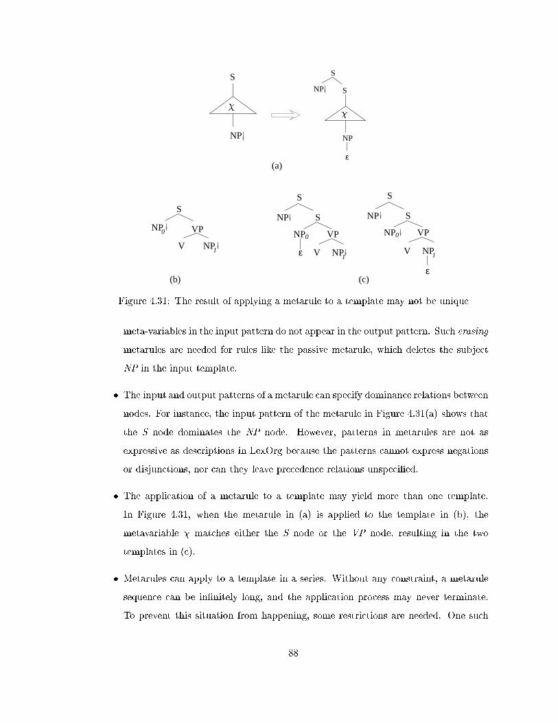
S
NP VP0
V NP1
S
NP VP
S
NP
ε
0
V NP1
S
NP
S
NP
ε
S
NP
S
NP VP
S
NP
0
V NP1
ε(c)(b)
(a)
��
Figure 4.31: The result of applying a metarule to a template may not be unique
meta-variables in the input pattern do not appear in the output pattern. Such erasing
metarules are needed for rules like the passive metarule, which deletes the subject
NP in the input template.
� The input and output patterns of a metarule can specify dominance relations between
nodes. For instance, the input pattern of the metarule in Figure 4.31(a) shows that
the S node dominates the NP node. However, patterns in metarules are not as
expressive as descriptions in LexOrg because the patterns cannot express negations
or disjunctions, nor can they leave precedence relations unspeci�ed.
� The application of a metarule to a template may yield more than one template.
In Figure 4.31, when the metarule in (a) is applied to the template in (b), the
metavariable � matches either the S node or the VP node, resulting in the two
templates in (c).
� Metarules can apply to a template in a series. Without any constraint, a metarule
sequence can be in�nitely long, and the application process may never terminate.
To prevent this situation from happening, some restrictions are needed. One such
88
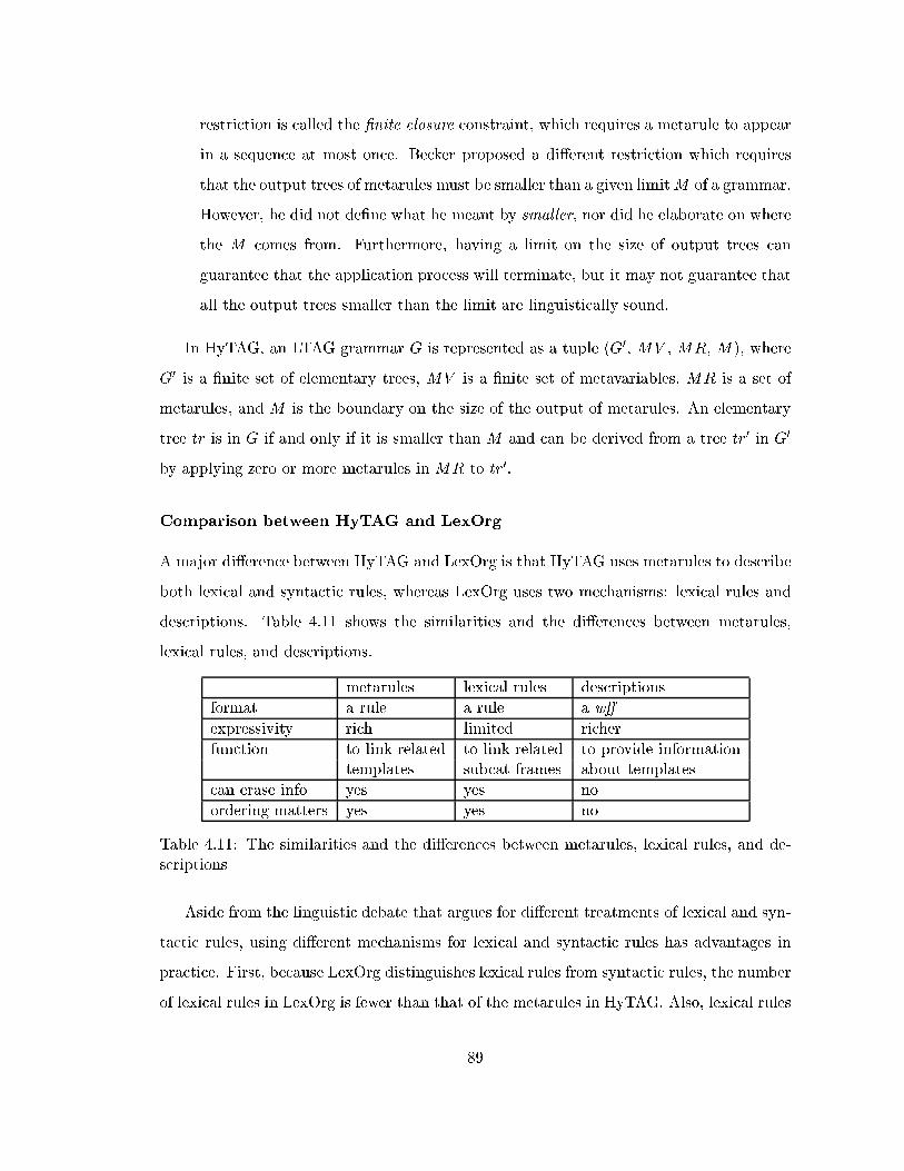
restriction is called the �nite closure constraint, which requires a metarule to appear
in a sequence at most once. Becker proposed a di�erent restriction which requires
that the output trees of metarules must be smaller than a given limitM of a grammar.
However, he did not de�ne what he meant by smaller, nor did he elaborate on where
the M comes from. Furthermore, having a limit on the size of output trees can
guarantee that the application process will terminate, but it may not guarantee that
all the output trees smaller than the limit are linguistically sound.
In HyTAG, an LTAG grammar G is represented as a tuple (G0, MV , MR, M), where
G0 is a �nite set of elementary trees, MV is a �nite set of metavariables, MR is a set of
metarules, and M is the boundary on the size of the output of metarules. An elementary
tree tr is in G if and only if it is smaller than M and can be derived from a tree tr0 in G0
by applying zero or more metarules in MR to tr0.
Comparison between HyTAG and LexOrg
A major di�erence between HyTAG and LexOrg is that HyTAG uses metarules to describe
both lexical and syntactic rules, whereas LexOrg uses two mechanisms: lexical rules and
descriptions. Table 4.11 shows the similarities and the di�erences between metarules,
lexical rules, and descriptions.
metarules lexical rules descriptions
format a rule a rule a w�
expressivity rich limited richer
function to link related to link related to provide informationtemplates subcat frames about templates
can erase info yes yes no
ordering matters yes yes no
Table 4.11: The similarities and the di�erences between metarules, lexical rules, and de-scriptions
Aside from the linguistic debate that argues for di�erent treatments of lexical and syn-
tactic rules, using di�erent mechanisms for lexical and syntactic rules has advantages in
practice. First, because LexOrg distinguishes lexical rules from syntactic rules, the number
of lexical rules in LexOrg is fewer than that of the metarules in HyTAG. Also, lexical rules
89

are much simpler than metarules because there are no metavariables in lexical rules. As
a result, it is easier to ensure the termination of the application process when the rules
are lexical rules rather than metarules. Second, lexical rules are more idiosyncratic than
syntactic rules. For instance, the causative/inchoative alternation only applies to ergative
verbs, rather than to all the transitive verbs, whereas any verb with an NP argument
anchors an elementary tree in which the NP argument undergoes wh-movement. To rep-
resent such idiosyncrasy, Becker proposed that the grammar developers \state for each
entry in the (syntactic) lexicon and for each tree family in this entry, which metarules
are applicable for this entry in this tree family". If LexOrg adopted this approach, the
grammar developers (i.e., the users of LexOrg) would specify only the lexical rules that
are applicable, and not the syntactic rules. Syntactic rules are represented by syntactic
variation descriptions, whose applicability is checked by the Tree Generator automatically
and therefore does not needed to be speci�ed by grammar developers.
Another di�erence between HyTAG and LexOrg is the way templates are related. For
the templates in the same tree family, the users of HyTAG �rst build one template as
the basic tree, and then create metarules that link the basic tree and other trees in the
family. When creating a metarule m, the users should consider all the templates t1 to
which m is applied and all the templates t2 that are to be generated from t1 when m is
applied. The users have to specify in the input pattern all the information that is in t1
but not in t2, and specify in the output pattern all the information that is in t2 but not in
t1. For example, the users may choose the tree for declarative sentences as the basic tree,
and then build metarules to derive the trees for imperative, wh-movement, and so on. If
there is information that is in the declarative tree but not in other trees, the users have to
repeat this information in all the input patterns of the metarules that are applied to the
declarative tree. In contrast, the users of LexOrg provide a subcategorization frame and
a set of descriptions. For each tree in the tree family, the Description Selector of LexOrg
chooses the same set of subcategorization descriptions (according to the subcategorization
frame) but a di�erent set of syntactic variation and modi�cation descriptions. The trees
are related by the descriptions that they share, rather than by some rules that link them
explicitly. Figure 4.32 illustrates these two di�erent approaches. In this �gure, mi are
90

4 5 6 7d d d d d9d81 2 3
t 1
2t
t3
m2
4t
m3
1m m
4 t5
t6
t7
m6
5m
t t tttt t1 2 3 4 5 6 7
d d d
modificationsubcategorization transformationdescriptions descriptionsdescriptions
(a) HyTAG (b) LexOrg
Input: t1 and fmigOutput: fti j i > 1g
Input: a subcat frame and fdigOutput: ftig and the lines between fdig and ftig
Figure 4.32: The ways that templates in a tree family are related in two systems
metarules, ti are templates, and di are descriptions. The inputs to HyTAG are t1 and fmig,and the inputs to LexOrg are fdig and a subcategorization frame. LexTract generates all
the templates, whereas HyTAG generates all but t1.
For templates in two related tree families, HyTAG uses a metarule to link the basic
trees in the tree families. Once again, the input and output patterns have to specify
what information is in one tree but not in the other. Figure 4.33(a) shows a metarule
that links the transitive tree and the ergative tree. In the transitive tree, the surface
subject is NP0 and the subject-verb agreement is between NP0 and V P , whereas in the
ergative tree the surface subject is NP1 and the subject-verb agreement is between NP1
and V P . To get it right, the metarule has to specify the agreement features in both sides
of the metarule, although the agreement is always between the surface subject and the VP
and it has nothing to do with the causative/inchoative alternation. In contrast, to relate
templates in two tree families, LexOrg uses a lexical rule to link two subcategorization
frames of the tree families, which is much simpler than a metarule. In this example, the
lexical rule (see Figure 4.33(b)) does not include subject-verb agreement features because
for both subcategorization frames LexOrg will select a description head V has left NP arg,
in which the agreement feature is speci�ed.
91
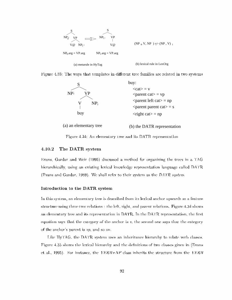
S
NP VP
V@ NP
0
1
NP .arg = VP.arg0
NP VP
S
V@
1
NP .arg = VP.arg1
(a) metarule in HyTag (b) lexical rule in LexOrg
(NP , V, NP ) => (NP , V)0 1 1
Figure 4.33: The ways that templates in di�erent tree families are related in two systems
S
NP VP
V NP
buy
(a) an elementary tree
buy:
<cat> = v<parent cat> = vp
<parent left cat> = np
<parent parent cat> = s
<right cat> = np
(b) the DATR representation
Figure 4.34: An elementary tree and its DATR representation
4.10.2 The DATR system
Evans, Gazdar and Weir (1995) discussed a method for organizing the trees in a TAG
hierarchically, using an existing lexical knowledge representation language called DATR
(Evans and Gazdar, 1989). We shall refer to their system as the DATR system.
Introduction to the DATR system
In this system, an elementary tree is described from its lexical anchor upwards as a feature
structure using three tree relations : the left, right, and parent relations. Figure 4.34 shows
an elementary tree and its representation in DATR. In the DATR representation, the �rst
equation says that the category of the anchor is v, the second one says that the category
of the anchor's parent is vp, and so on.
Like HyTAG, the DATR system uses an inheritance hierarchy to relate verb classes.
Figure 4.35 shows the lexical hierarchy and the de�nitions of two classes given in (Evans
et al., 1995). For instance, the VERB+NP class inherits the structure from the VERB
92
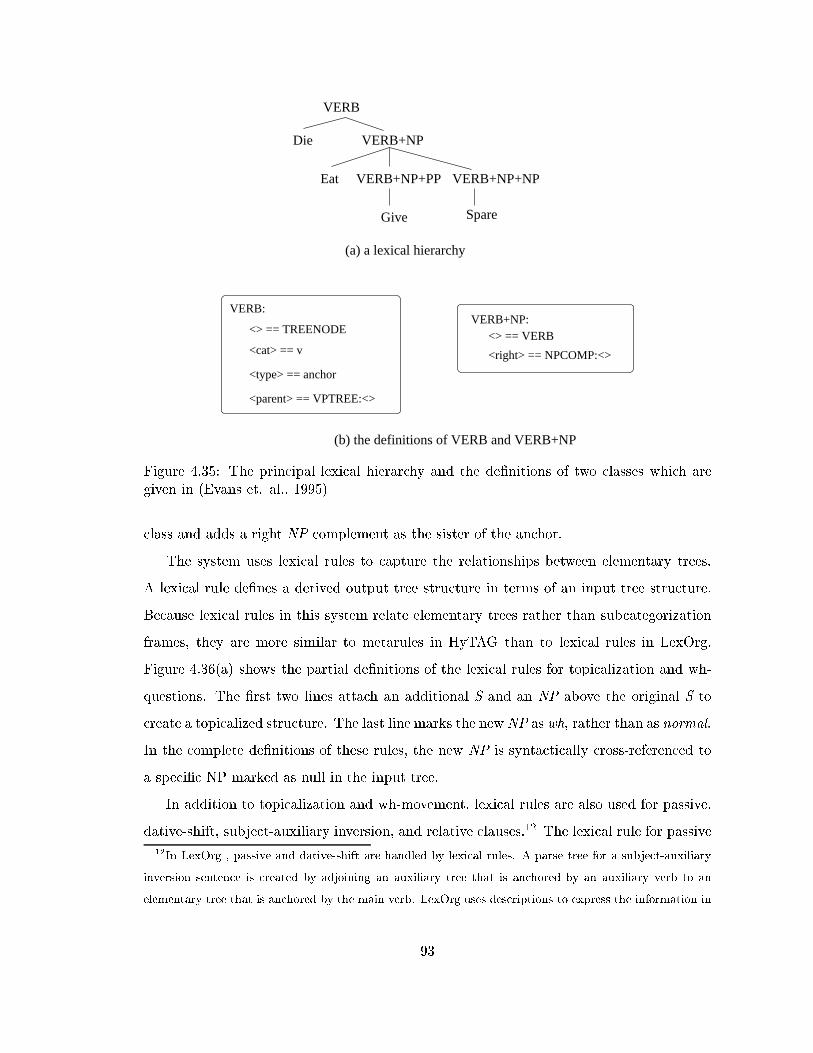
VERB
Die VERB+NP
VERB+NP+PP VERB+NP+NP
SpareGive
Eat
VERB:
<> == TREENODE
<cat> == v
<type> == anchor
<parent> == VPTREE:<>
VERB+NP:<> == VERB
<right> == NPCOMP:<>
(a) a lexical hierarchy
(b) the definitions of VERB and VERB+NP
Figure 4.35: The principal lexical hierarchy and the de�nitions of two classes which aregiven in (Evans et. al., 1995)
class and adds a right NP complement as the sister of the anchor.
The system uses lexical rules to capture the relationships between elementary trees.
A lexical rule de�nes a derived output tree structure in terms of an input tree structure.
Because lexical rules in this system relate elementary trees rather than subcategorization
frames, they are more similar to metarules in HyTAG than to lexical rules in LexOrg.
Figure 4.36(a) shows the partial de�nitions of the lexical rules for topicalization and wh-
questions. The �rst two lines attach an additional S and an NP above the original S to
create a topicalized structure. The last line marks the newNP as wh, rather than as normal.
In the complete de�nitions of these rules, the new NP is syntactically cross-referenced to
a speci�c NP marked as null in the input tree.
In addition to topicalization and wh-movement, lexical rules are also used for passive,
dative-shift, subject-auxiliary inversion, and relative clauses.12 The lexical rule for passive
12In LexOrg , passive and dative-shift are handled by lexical rules. A parse tree for a subject-auxiliary
inversion sentence is created by adjoining an auxiliary tree that is anchored by an auxiliary verb to an
elementary tree that is anchored by the main verb. LexOrg uses descriptions to express the information in
93
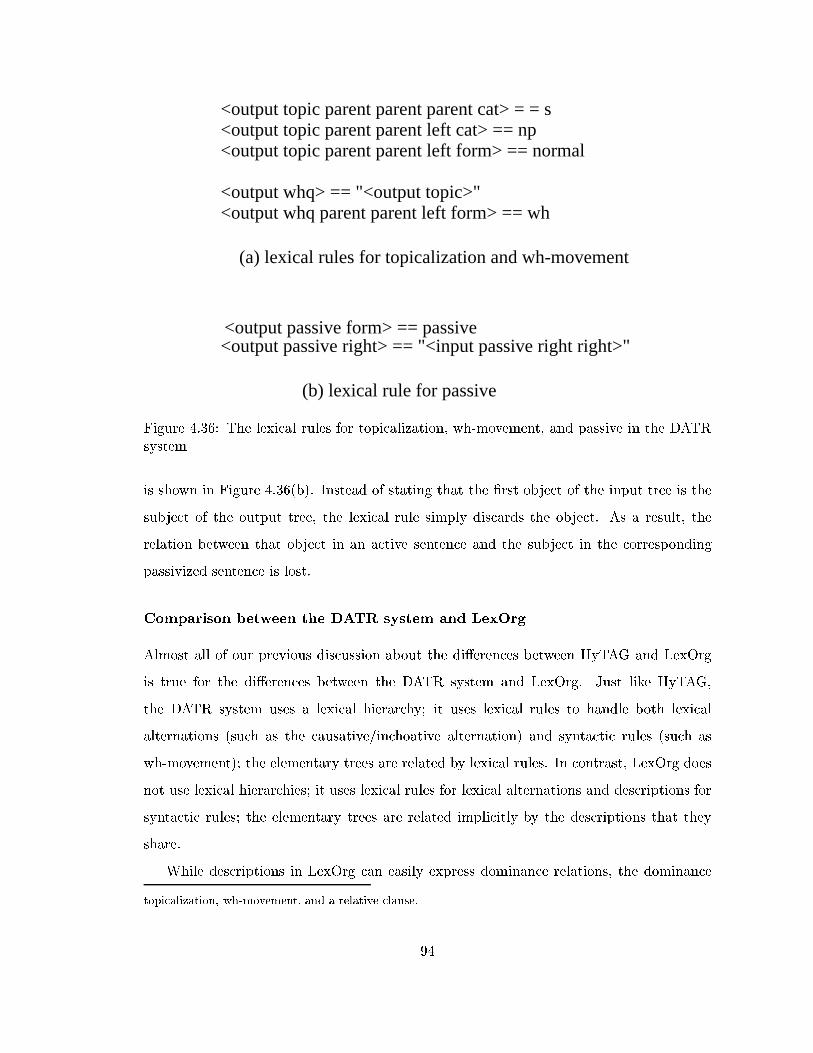
<output topic parent parent parent cat> = = s<output topic parent parent left cat> == np<output topic parent parent left form> == normal
<output whq> == "<output topic>"<output whq parent parent left form> == wh
(b) lexical rule for passive
(a) lexical rules for topicalization and wh-movement
<output passive form> == passive<output passive right> == "<input passive right right>"
Figure 4.36: The lexical rules for topicalization, wh-movement, and passive in the DATRsystem
is shown in Figure 4.36(b). Instead of stating that the �rst object of the input tree is the
subject of the output tree, the lexical rule simply discards the object. As a result, the
relation between that object in an active sentence and the subject in the corresponding
passivized sentence is lost.
Comparison between the DATR system and LexOrg
Almost all of our previous discussion about the di�erences between HyTAG and LexOrg
is true for the di�erences between the DATR system and LexOrg. Just like HyTAG,
the DATR system uses a lexical hierarchy; it uses lexical rules to handle both lexical
alternations (such as the causative/inchoative alternation) and syntactic rules (such as
wh-movement); the elementary trees are related by lexical rules. In contrast, LexOrg does
not use lexical hierarchies; it uses lexical rules for lexical alternations and descriptions for
syntactic rules; the elementary trees are related implicitly by the descriptions that they
share.
While descriptions in LexOrg can easily express dominance relations, the dominance
topicalization, wh-movement, and a relative clause.
94
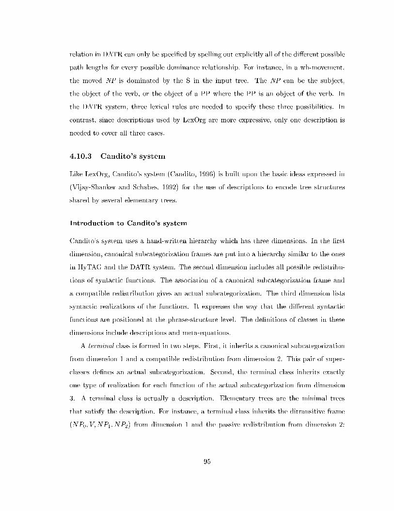
relation in DATR can only be speci�ed by spelling out explicitly all of the di�erent possible
path lengths for every possible dominance relationship. For instance, in a wh-movement,
the moved NP is dominated by the S in the input tree. The NP can be the subject,
the object of the verb, or the object of a PP where the PP is an object of the verb. In
the DATR system, three lexical rules are needed to specify these three possibilities. In
contrast, since descriptions used by LexOrg are more expressive, only one description is
needed to cover all three cases.
4.10.3 Candito's system
Like LexOrg, Candito's system (Candito, 1996) is built upon the basic ideas expressed in
(Vijay-Shanker and Schabes, 1992) for the use of descriptions to encode tree structures
shared by several elementary trees.
Introduction to Candito's system
Candito's system uses a hand-written hierarchy which has three dimensions. In the �rst
dimension, canonical subcategorization frames are put into a hierarchy similar to the ones
in HyTAG and the DATR system. The second dimension includes all possible redistribu-
tions of syntactic functions. The association of a canonical subcategorization frame and
a compatible redistribution gives an actual subcategorization. The third dimension lists
syntactic realizations of the functions. It expresses the way that the di�erent syntactic
functions are positioned at the phrase-structure level. The de�nitions of classes in these
dimensions include descriptions and meta-equations.
A terminal class is formed in two steps. First, it inherits a canonical subcategorization
from dimension 1 and a compatible redistribution from dimension 2. This pair of super-
classes de�nes an actual subcategorization. Second, the terminal class inherits exactly
one type of realization for each function of the actual subcategorization from dimension
3. A terminal class is actually a description. Elementary trees are the minimal trees
that satisfy the description. For instance, a terminal class inherits the ditransitive frame
(NP0; V;NP1; NP2) from dimension 1 and the passive redistribution from dimension 2;
95
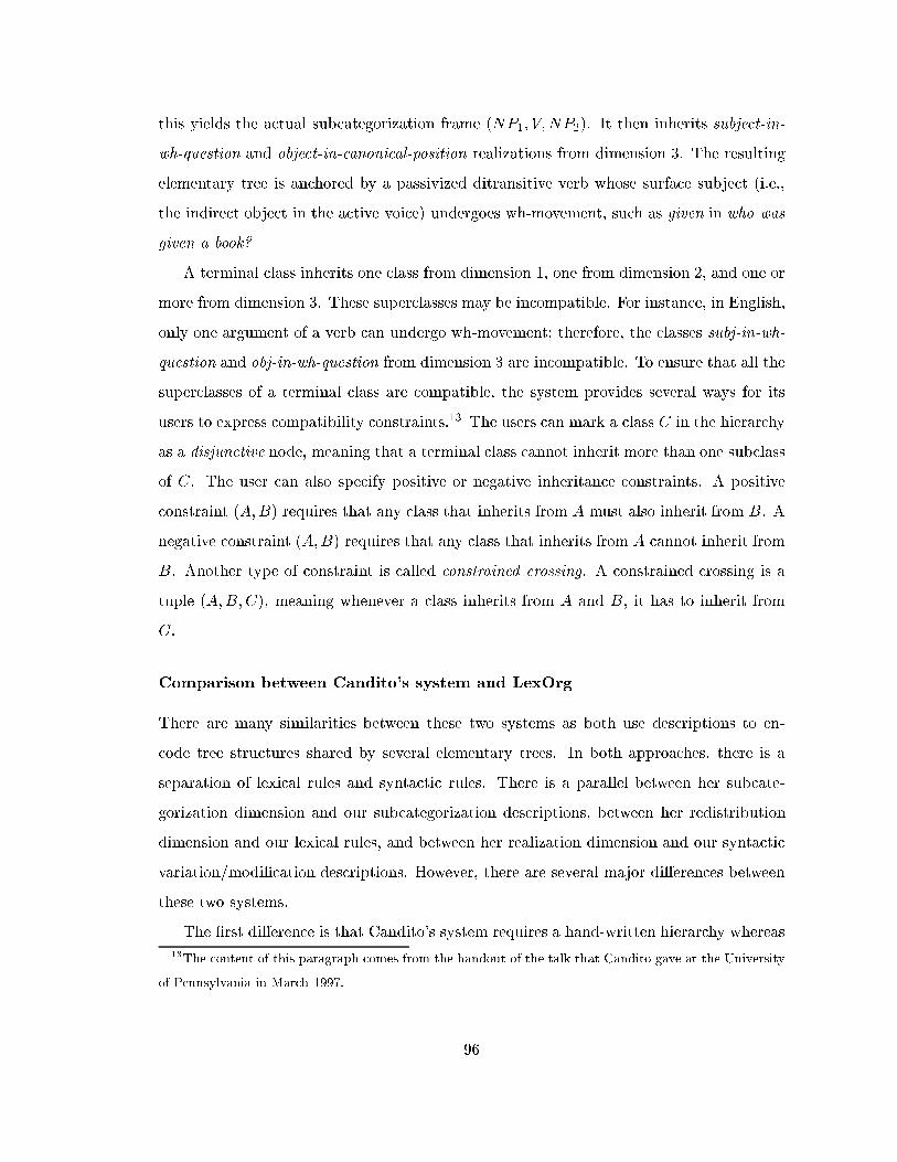
this yields the actual subcategorization frame (NP1; V;NP2). It then inherits subject-in-
wh-question and object-in-canonical-position realizations from dimension 3. The resulting
elementary tree is anchored by a passivized ditransitive verb whose surface subject (i.e.,
the indirect object in the active voice) undergoes wh-movement, such as given in who was
given a book?
A terminal class inherits one class from dimension 1, one from dimension 2, and one or
more from dimension 3. These superclasses may be incompatible. For instance, in English,
only one argument of a verb can undergo wh-movement; therefore, the classes subj-in-wh-
question and obj-in-wh-question from dimension 3 are incompatible. To ensure that all the
superclasses of a terminal class are compatible, the system provides several ways for its
users to express compatibility constraints.13 The users can mark a class C in the hierarchy
as a disjunctive node, meaning that a terminal class cannot inherit more than one subclass
of C. The user can also specify positive or negative inheritance constraints. A positive
constraint (A;B) requires that any class that inherits from A must also inherit from B. A
negative constraint (A;B) requires that any class that inherits from A cannot inherit from
B. Another type of constraint is called constrained crossing. A constrained crossing is a
tuple (A;B;C), meaning whenever a class inherits from A and B, it has to inherit from
C.
Comparison between Candito's system and LexOrg
There are many similarities between these two systems as both use descriptions to en-
code tree structures shared by several elementary trees. In both approaches, there is a
separation of lexical rules and syntactic rules. There is a parallel between her subcate-
gorization dimension and our subcategorization descriptions, between her redistribution
dimension and our lexical rules, and between her realization dimension and our syntactic
variation/modi�cation descriptions. However, there are several major di�erences between
these two systems.
The �rst di�erence is that Candito's system requires a hand-written hierarchy whereas
13The content of this paragraph comes from the handout of the talk that Candito gave at the University
of Pennsylvania in March 1997.
96
LexOrg does not. We have mentioned that LexOrg can automatically generate a lexical
hierarchy | which is similar to Candito's dimension 1 | when given a set of subcatego-
rization frames. As for dimension 2, Candito's system requires that each terminal class
should select exactly one class from this dimension. This means that if two lexical rules
can be applied in a series (such as passive and causative) to a subcategorization frame, a
node that represents that sequence must be manually created and added to her dimension
2. In other words, her dimension 2 should have a node for every lexical-rule sequence that
is applicable to some subcategorization frame. LexOrg does not need users to build this
dimension manually because LexOrg (the Frame Generator, to be more precise) automat-
ically tries all the lexical-rule sequences when given a subcategorization frame.
The two systems also di�er in the way that syntactic variations are represented. In
Candito's third dimension, each terminal node speci�es the way a speci�c function is real-
ized. Therefore, each argument/function in a subcategorization frame requires a terminal
node for each possible syntactic realization. For example, the subject of a ditransitive verb
has a di�erent terminal node for the canonical position, for wh-extraction, and so on. So
do the direct object and indirect object. To generate templates for wh-questions of ditran-
sitive verbs, Candito's system needs to build three terminal classes, as shown in Figure
4.37(a). In contrast, LexOrg does not need descriptions for various positions that each
argument/function can be in. It only needs one description for wh-movement. To generate
the template for wh-questions, LexOrg only needs one wh-movement description from this
dimension. Combining this description with the set of subcategorization descriptions will
yield all the templates for wh-questions, as in Figure 4.37(b).
Another di�erence between the two systems is that Candito's system requires its users
to specify constraints on the selection of superclasses. For instance, the user has to build a
class for wh-movement and a subclass for each position from which a constituent is moved
(e.g., subj-in-wh-position, indobj-in-wh-question, and dobj-in-wh-question). The users then
have to mark the extraction class as a disjunctive node, so that the system will not choose
more than one of its children for a terminal class. In LexOrg, only one description for
wh-movement is needed, which covers all possible cases of wh-movement. The description
appears in a description set at most once. As a result, there is no need to write constraints
97

#2:
#3:
#4:
#5:
#6:
#7:
indobj-in-wh-question
indobj-in-canon-pos
subj-in-wh-quest
subj-in-canon-pos#1: subcat desc
#1 + #3 + #4 + #6 => wh-subj
dobj-in-canon-pos
dobj-in-wh-question
#1 + #2 + #5 + #6 => wh-indobj
#1 + #2 + #4 + #7 => wh-dobj
(a) Candito’s system
#1’: subcat desc
#2’: wh-movement
wh-dobj
wh-subj#1’ + #2’ => wh-indobj
(b) LexOrg
Figure 4.37: The di�erent ways that two systems handle wh-movement
to rule out illegal combinations such as the ones with both subj-in-wh-position and indobj-
in-wh-question.
In summary, LexOrg has several advantages over other systems. First, unlike all three
other systems, not only does LexOrg not require its users to build any lexical hierarchy,
but it can actually produce a hierarchy automatically by checking the descriptions selected
by subcategorization frames. Second, unlike HyTAG and the DATR system, LexOrg dis-
tinguishes lexical rules from syntactic rules and uses two di�erent mechanisms to represent
these rules. Making such distinction has advantages both in theory and in practice. Third,
unlike Candito's system, LexOrg does not require users to provide various kinds of con-
straints to ensure that a terminal class inherits the correct combinations of superclasses
from three dimensions. Fourth, unlike the DATR system and the Candito's system, LexOrg
needs only one description to specify the information for wh-movement.
4.11 Summary
In summary, we have presented a system, LexOrg, that takes three types of information
(i.e., subcategorization frames, lexical rules, and descriptions) as input and produces LTAG
grammars as output. Descriptions are further divided into four types according to the
information that they provide. The abstract level of representation for the grammar both
98

necessitates and facilitates an examination of the linguistic analyses. This can be very
useful for gaining an overview of the theory that is being implemented and exposing gaps
that remain unmotivated and need to be investigated. We have used LexOrg to build
grammars for English and Chinese. We also showed that LexOrg has several advantages
over other systems.
99
Chapter 5
LexTract: a system that extracts
LTAGs from Treebanks
In Chapter 3, we gave an algorithm that generates a grammar, GTable, from three tables |
the head projection table, the argument table, and the modi�cation table. The grammar
overgenerates because the tables do not provide suÆcient information about a language.
In Chapter 4, we presented a system, LexOrg, that solves this problem by requesting
more informative input (such as descriptions) from its users. Creating such input requires
linguistic expertise. Furthermore, there is no frequency information associated with the
grammars produced by LexOrg. To use the grammars for parsing, other sources of infor-
mation (such as heuristic rules) have to be found to help us select the most likely parse
trees.
To address these problems, we built another system, called LexTract. LexTract takes
a Treebank and three tables as input and produces as output LTAG grammars, derivation
trees and other types of information, as shown in Figure 5.1. The system has been used
in a number of applications. In this chapter, we describe core components of the system,
and leave the discussion of its applications to the next chapter.
This chapter is organized as follows. In Section 5.1, we give a brief introduction to
the English Penn Treebank, which is widely used in the NLP �eld. In Section 5.2, we
describe the overall approach of LexTract. In Section 5.3, we discuss three input tables to
100

LexTract
Treebank
Language-specificinformation
Derivation trees
LTAGs
CFGs
MC sets
Figure 5.1: Architecture of LexTract
LexTract. In Section 5.4, we give an algorithm that extracts grammars from Treebanks.
In Section 5.5, we describe a method for building derivation trees for the sentences in the
Treebank. In Section 5.6, we demonstrate the process for building the multi-component
(MC) sets from derivation trees. In Section 5.7, we show that context-free grammars and
subcategorization information can be easily obtained from extracted LTAGs. In Section
5.8, we explain our treatment for several special cases. In Section 5.9, we compare LexTract
with other grammar extraction methods.
5.1 Overview of the English Penn Treebank
The English Penn Treebank (PTB) is widely used in the NLP community for training and
testing statistical tools such as POS taggers and parsers. It is also the �rst Treebank on
which LexTract was used. Therefore, we shall use examples from the PTB throughout this
chapter to demonstrate how LexTract works. The PTB was developed at the University
of Pennsylvania in the early 1990s. It includes about one million words of text from the
Wall Street Journal annotated in Treebank II style (Marcus et al., 1994). Its tagset has 72
syntactic labels (36 POS tags, 26 syntactic category tags, 10 tags for empty categories1)
and 20 function tags. Each bracketed item is labeled with one syntactic category, zero
or more function tags, and zero or more reference indices. For details, please refer to
(Santorini, 1990) and (Bies et al., 1995). The meanings of the tags that appear in this
chapter are listed in Table 5.1. Figure 5.2 is a simple example that shall be used throughout
1The PTB uses -NONE- for all empty categories, but it also uses 10 more speci�c tags to mark di�erent
types of empty categories. For example, a trace is marked as (-NONE- *T*-1), where -1 can be replaced
by any reference index.
101
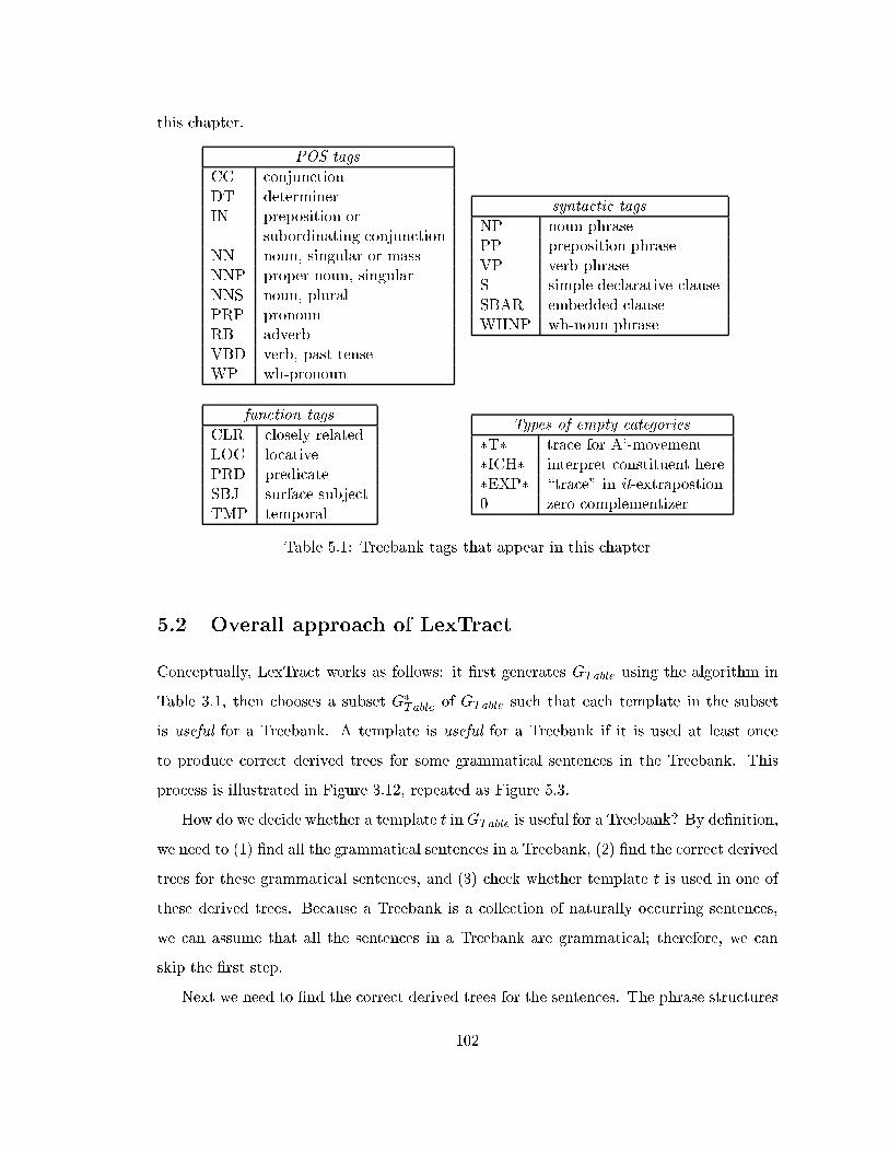
this chapter.
POS tags
CC conjunctionDT determinerIN preposition or
subordinating conjunctionNN noun, singular or massNNP proper noun, singularNNS noun, pluralPRP pronounRB adverbVBD verb, past tenseWP wh-pronoun
syntactic tags
NP noun phrasePP preposition phraseVP verb phraseS simple declarative clauseSBAR embedded clauseWHNP wh-noun phrase
function tags
CLR closely relatedLOC locativePRD predicateSBJ surface subjectTMP temporal
Types of empty categories
�T� trace for A'-movement�ICH� interpret constituent here�EXP� \trace" in it-extrapostion0 zero complementizer
Table 5.1: Treebank tags that appear in this chapter
5.2 Overall approach of LexTract
Conceptually, LexTract works as follows: it �rst generates GTable using the algorithm in
Table 3.1, then chooses a subset G�Table of GTable such that each template in the subset
is useful for a Treebank. A template is useful for a Treebank if it is used at least once
to produce correct derived trees for some grammatical sentences in the Treebank. This
process is illustrated in Figure 3.12, repeated as Figure 5.3.
How do we decide whether a template t inGTable is useful for a Treebank? By de�nition,
we need to (1) �nd all the grammatical sentences in a Treebank, (2) �nd the correct derived
trees for these grammatical sentences, and (3) check whether template t is used in one of
these derived trees. Because a Treebank is a collection of naturally occurring sentences,
we can assume that all the sentences in a Treebank are grammatical; therefore, we can
skip the �rst step.
Next we need to �nd the correct derived trees for the sentences. The phrase structures
102
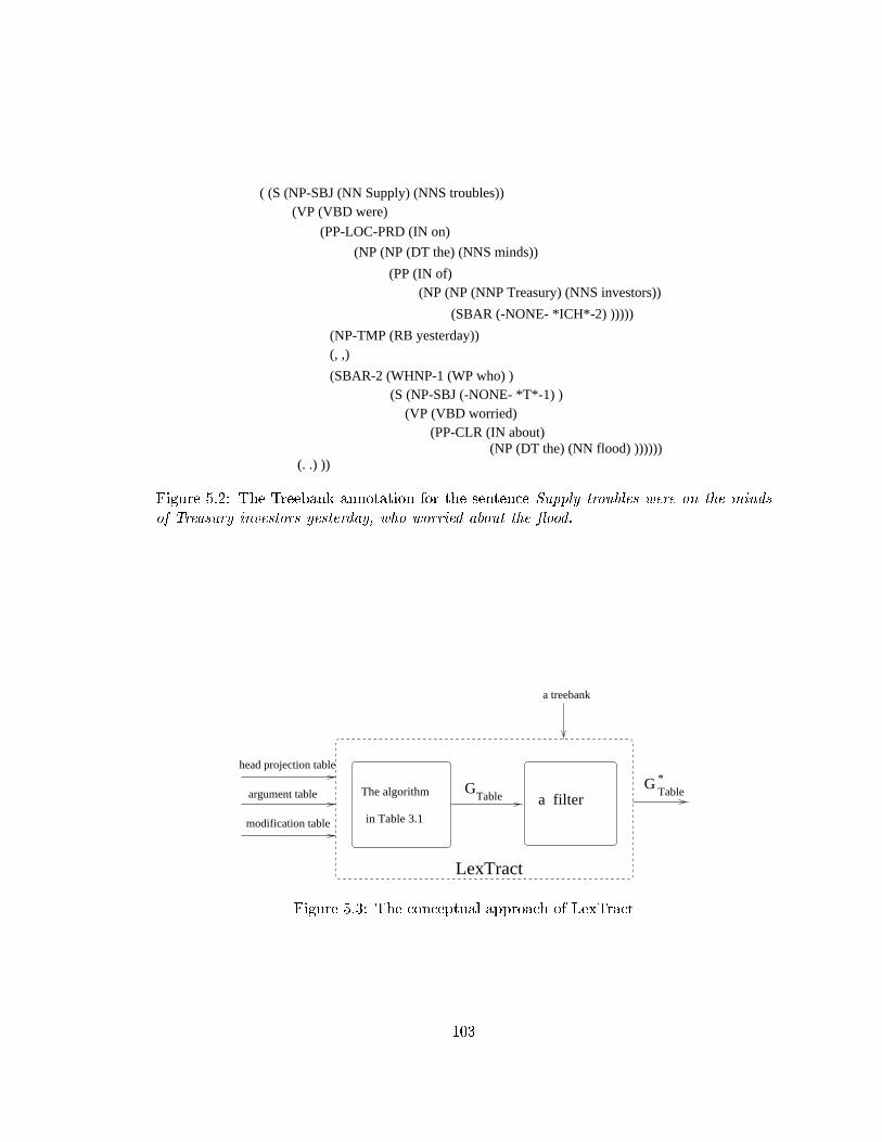
( (S (NP-SBJ (NN Supply) (NNS troubles))(VP (VBD were)
(PP-LOC-PRD (IN on)
(NP (NP (DT the) (NNS minds))
(PP (IN of)(NP (NP (NNP Treasury) (NNS investors))
(SBAR (-NONE- *ICH*-2) )))))
(NP-TMP (RB yesterday))(, ,)
(SBAR-2 (WHNP-1 (WP who) ) (S (NP-SBJ (-NONE- *T*-1) ) (VP (VBD worried) (PP-CLR (IN about)
(. .) )) (NP (DT the) (NN flood) ))))))
Figure 5.2: The Treebank annotation for the sentence Supply troubles were on the mindsof Treasury investors yesterday, who worried about the ood.
The algorithm
in Table 3.1
GTable
G *Table
a filter
LexTract
head projection table
modification table
argument table
a treebank
Figure 5.3: The conceptual approach of LexTract
103

in a Treebank are not always identical to the correct parse trees because of two reasons.
First, Treebank were built by humans; therefore, annotation errors in a Treebank are
inevitable. Second, the phrase structures in a Treebank are not based on the LTAG
formalism; therefore, they may have di�erent formats from the derived trees. For instance,
LTAG grammars distinguish heads, argument, and adjuncts. Recall that in Section 3.2,
we de�ned three prototypes of elementary trees: spine-etrees, mod-etrees, and conj-etrees.
Heads, arguments, and adjuncts occur at di�erent positions in these prototypes. The
arguments and adjuncts are never siblings in an LTAG derived tree. In a Treebank, quite
often the arguments and adjuncts are siblings, and the head/argument/adjunct distinction
is not explicitly marked. Therefore, we have to convert the phrase structures in a Treebank
into derived trees.
Once we build derived trees, the next step is to determine what elementary trees are
used to form the derived tree. A derived tree can be generated by more than one set of ele-
mentary trees. Figure 5.5(b){(c) show two sets of elementary trees. Both sets can generate
the derived tree in (a), but the corresponding derivations are di�erent, as shown in (d) and
(e). Nevertheless, we shall show that, if we know the type (i.e., head/argument/adjunct)
of each node in a derived tree, there is only one set of elementary trees that can form the
derived tree. For instance, in Figure 5.5(a), if verb can is marked as the head of V P1, the
derived tree in (a) can only come from the set in (b); if verb speak is marked as the head of
V P1, the derived tree can only come from the set in (c). In fact, we can simply decompose
the derived tree into a set of elementary trees.
In summary, LexTract builds an LTAG grammar in two stages: �rst, it converts the
phrase structures in a Treebank into derived trees; second, it decomposes the derived trees
into a set of elementary trees. The second stage is the reverse process of LTAG parsing.
The real implementation of LexTract is shown in Figure 5.4. You may notice that the
three input tables in Figures 5.3 and 5.4 are di�erent. We shall explain this in the next
section.
For the sake of clarity, from now on, we shall call the original phrase structures in a
Treebank ttrees, and the elementary trees in LTAG grammars etrees.
104
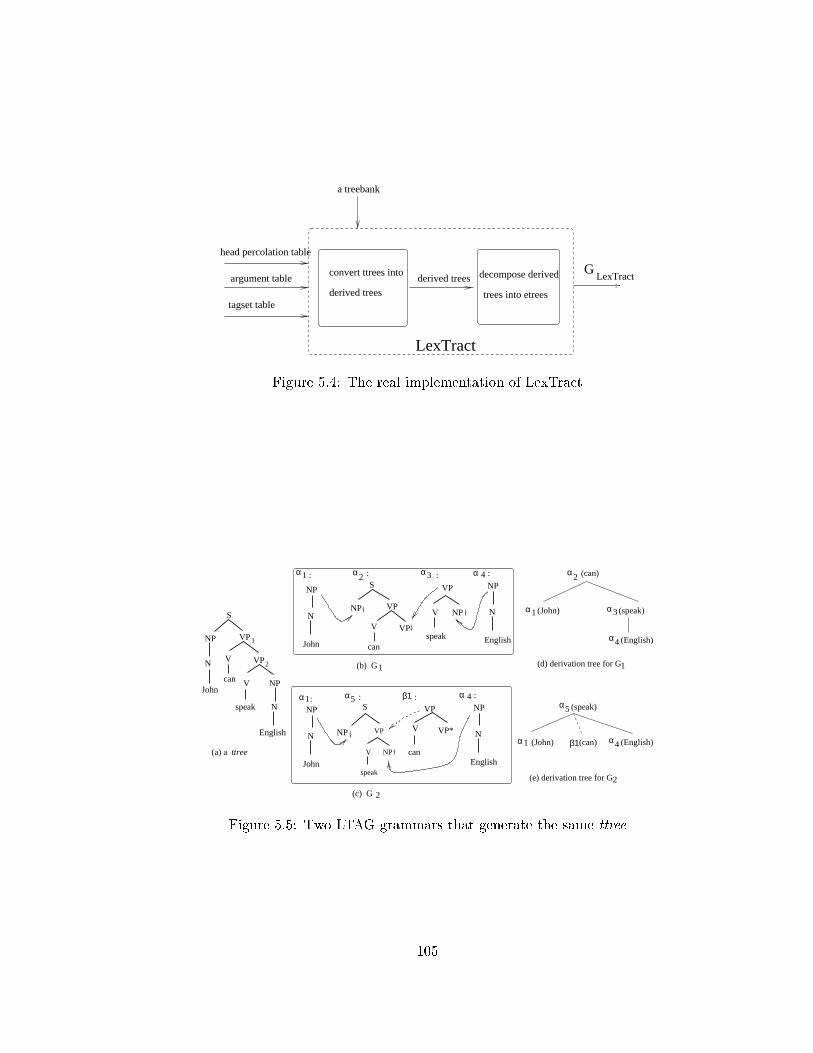
GLexTract
LexTract
tagset table
argument table
head percolation table
a treebank
derived treesconvert ttrees into
derived trees trees into etrees
decompose derived
Figure 5.4: The real implementation of LexTract
α1
NP
N
John
S
VPNP
V
can
VP
α2α1 α3
VP
V NP
speak
NP
N
John
VP
V NP
speak
β1
α 4 :
NP
N
English
α 4 :
NP
N
English
α2 (can)
α1 (John) α3
α4 (English)
α1 (John) β1(can) α4 (English)
α5 (speak)
(b) G1
(c) G 2
:
S
VP
VPV
canJohn
NP
N
V
speak
NP
N
English
ttree(a) a
:: :
:S
NP
:VP
V
can
VP*
α5
(speak)
(d) derivation tree for G1
(e) derivation tree for G2
1
2
Figure 5.5: Two LTAG grammars that generate the same ttree
105

5.3 Three input tables to LexTract
In the English Penn Treebank (PTB), the phrase structures are partially at because
heads, arguments and adjuncts are not explicitly marked, and arguments and adjuncts
can be siblings. In contrast, heads, arguments and adjuncts are treated di�erently in the
target grammars (i.e., the LTAG grammars that LexTract generates): heads are anchors
of spine-etrees, arguments are sisters of nodes on the spines, and adjuncts are sisters of
the foot nodes in mod-etrees.
To build a derived tree from a ttree, LexTract �rst determines the type of each node in
the ttree. People often do not agree on the types of certain nodes. For example, in Figure
5.5, some users may prefer to treat speak as the head of V P1, while others rather have
the word can as the head. To take the users' preferences into account and also to make
LexTract language independent so that it can run on Treebanks for other languages, we
do not include language-speci�c information or decisions on the head/argument/adjunct
distinction in the source code of LexTract. Instead, we require the users of LexTract
to provide three tables as input to LexTract. They are the head percolation table, the
argument table, and the tagset table.
5.3.1 Head percolation table
Head is an important notion in the target grammar, but it is not marked in the PTB. To
help LexTract to identify heads, the user needs to make a head percolation table. The
head percolation table was introduced in a statistical parser called SPATTER (Magerman,
1995), and later used in Collins' parsers (Collins, 1997) among others. It is called a head
percolation table because, in order for those parsers to extract lexicalized context-free rules
from a Treebank, the lexical items are percolated like features from the heads to their
various projections, as marked by the dashed lines in Figure 5.6(a).
Given a node X and its head Y in a ttree, each node on the path from X to Y is
called the head-child of its parent. For example, in Figure 5.6(a), the VBP node is the
head-child of the VP node, the VP is the head-child of the S node, and the NNP is the
head-child of the NP. LexTract uses the head percolation table to select the head-child
106

S(likes)
NP(John)
NNP(John)
John
VBP(likes) NP(apples)
NNS(apples)
apples
VP(likes) -> VBP(likes) NP(apples)NP(apples) -> NNS(apples)
NP(John) -> NNP (John)S(likes) -> NP(John) VP(likes)
VP(likes)
likes
(a) a ttree (b) a lexicalized CFG
Figure 5.6: The percolation of lexical items from heads to higher projections
of a node. The entry in the table is of the form (x direct y1=y2=:::=yn), where x and
yi are syntactic category tags, direct is either LEFT or RIGHT . fyig is the set of
possible tags of x's head-child. For instance, the entry for V P in the PTB can be (VP
left VP/VB/VBN/VBP/VBZ/VBG/VBD). The algorithm for selecting the head-child is
in Table 5.2 of Section 5.4. The head percolation table is essentially the same as the head
projection table except that it has an extra �eld direct.
5.3.2 Argument table
The argument/adjunct distinction is not explicitly marked in the PTB. LexTract marks
each sibling of a head-child as either an argument or an adjunct according to the tag of the
sibling, the tag of the head-child, and the position of the sibling with respect to the head-
child. An argument table informs LexTract about the types of arguments that a head-child
can take. As de�ned in Section 3.3, the entry in an argument table is of the form (head tag,
left arg num, right arg num, y1=y2=:::=yn). head tag is the syntactic tag of the head-child,
fyig is the set of possible tags for the head-child's arguments, left arg num (right arg num,
respectively.) is the maximal number of arguments to the left (right, respectively) of the
head-child. For example, the entry (IN, 0, 1, NP/S/SBAR) says that a preposition (IN)
can take at most one argument whose label is NP, S, or SBAR, and the argument appears
after the preposition. The algorithm for distinguishing arguments from adjuncts is shown
in Table 5.3 of Section 5.4.
107

5.3.3 Tagset table
The tagset table provides types and attributes of the tags in the Treebank's tagset, which
are used in many modules of LexTract. The most important attributes are as follows:
(1) the type of each tag in the tagset; namely, POS tag, syntactic tag, function tag, empty
category tag
(2) the tag(s) for conjunctions (e.g., CC in the PTB)
(3) the empty categories that mark \syntactic movement" (e.g., *T* for a trace)
(4) the function tags that always mark arguments (e.g., SBJ for a subject)
(5) the function tags that always mark adjuncts (e.g., TMP for a temporal phrase)
(6) the function tags that always mark heads (e.g., PRD for a predicate)
The last three attributes helps LexTract to make the head/argument/adjunct distinc-
tion. Recall that the algorithm in Table 3.1 which generates GTable requires the head
projection table, argument table, and modi�cation table. LexTract requires the head
percolation table, which has more information than the head projection table. LexTract
requires the argument table but not the modi�cation table because it assumes that any
category can modify any category. LexTract uses the tagset table to determine how the
function tags should be treated. Therefore, the three input tables to LexTract provide
more information than the three input tables to the algorithm that generates GTable. For
more details on all �ve types of tables, see Appendix A.
5.4 Extracting LTAG grammars from Treebanks
As discussed in Section 5.2, LexTract builds grammars in two stages: �rst, LexTract
converts a ttree into a derived tree; second, it decomposes the derived tree into a set of
etrees. In this section, we describe each stage in detail.
108
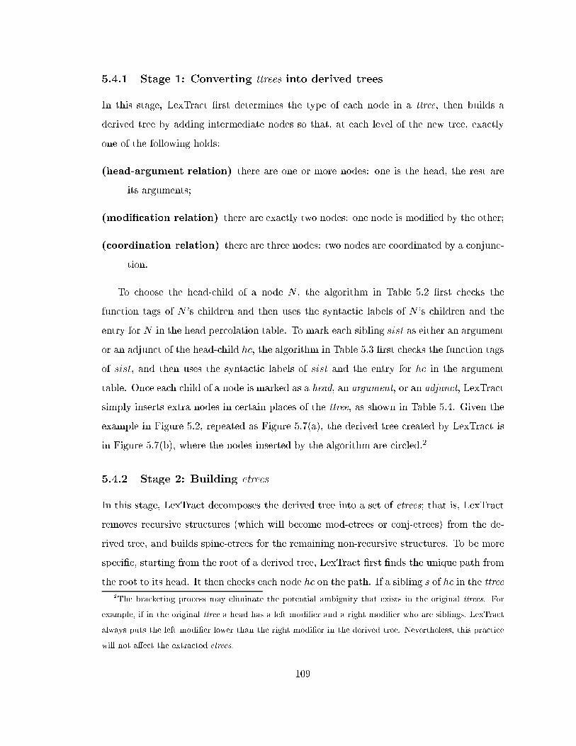
5.4.1 Stage 1: Converting ttrees into derived trees
In this stage, LexTract �rst determines the type of each node in a ttree, then builds a
derived tree by adding intermediate nodes so that, at each level of the new tree, exactly
one of the following holds:
(head-argument relation) there are one or more nodes: one is the head, the rest are
its arguments;
(modi�cation relation) there are exactly two nodes: one node is modi�ed by the other;
(coordination relation) there are three nodes: two nodes are coordinated by a conjunc-
tion.
To choose the head-child of a node N , the algorithm in Table 5.2 �rst checks the
function tags of N 's children and then uses the syntactic labels of N 's children and the
entry for N in the head percolation table. To mark each sibling sist as either an argument
or an adjunct of the head-child hc, the algorithm in Table 5.3 �rst checks the function tags
of sist, and then uses the syntactic labels of sist and the entry for hc in the argument
table. Once each child of a node is marked as a head, an argument, or an adjunct, LexTract
simply inserts extra nodes in certain places of the ttree, as shown in Table 5.4. Given the
example in Figure 5.2, repeated as Figure 5.7(a), the derived tree created by LexTract is
in Figure 5.7(b), where the nodes inserted by the algorithm are circled.2
5.4.2 Stage 2: Building etrees
In this stage, LexTract decomposes the derived tree into a set of etrees; that is, LexTract
removes recursive structures (which will become mod-etrees or conj-etrees) from the de-
rived tree, and builds spine-etrees for the remaining non-recursive structures. To be more
speci�c, starting from the root of a derived tree, LexTract �rst �nds the unique path from
the root to its head. It then checks each node hc on the path. If a sibling s of hc in the ttree
2The bracketing process may eliminate the potential ambiguity that exists in the original ttrees. For
example, if in the original ttree a head has a left modi�er and a right modi�er who are siblings, LexTract
always puts the left modi�er lower than the right modi�er in the derived tree. Nevertheless, this practice
will not a�ect the extracted etrees.
109
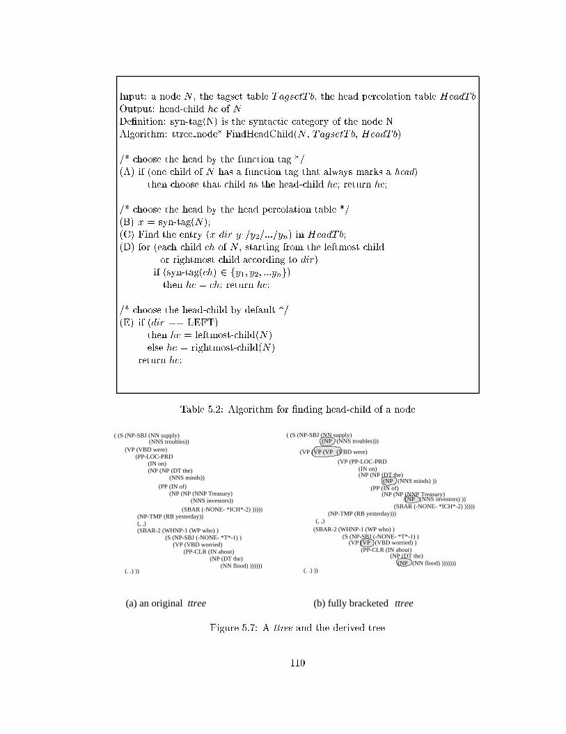
Input: a node N , the tagset table TagsetT b, the head percolation table HeadTbOutput: head-child hc of NDe�nition: syn-tag(N) is the syntactic category of the node NAlgorithm: ttree node* FindHeadChild(N , TagsetT b, HeadTb)
/* choose the head by the function tag */(A) if (one child of N has a function tag that always marks a head)
then choose that child as the head-child hc; return hc;
/* choose the head by the head percolation table */(B) x = syn-tag(N);(C) Find the entry (x dir y1=y2=:::=yn) in HeadTb;(D) for (each child ch of N , starting from the leftmost child
or rightmost child according to dir)if (syn-tag(ch) 2 fy1; y2; :::yng)then hc = ch; return hc;
/* choose the head-child by default */(E) if (dir == LEFT)
then hc = leftmost-child(N)else hc = rightmost-child(N)
return hc;
Table 5.2: Algorithm for �nding head-child of a node
( (S (NP-SBJ (NN supply)
(VP (VP (VP
(NP (NNS troubles)))
(VP (PP-LOC-PRD
(VBD were)
(IN on)(NP (NP (DT the)
(NP (NNS minds) ))(PP (IN of)
(NP (NP (NNP Treasury) (NP (NNS investors) ))
(SBAR (-NONE- *ICH*-2) )))))(NP-TMP (RB yesterday)))
(, ,)(SBAR-2 (WHNP-1 (WP who) ) (S (NP-SBJ (-NONE- *T*-1) )
(VP (VP (VBD worried) )(PP-CLR (IN about)
(NP (DT the) (NP (NN flood) )))))))
(. .) ))
(a) an original (b) fully bracketed ttreettree
(SBAR (-NONE- *ICH*-2) )))))
(VP (VBD were) (PP-LOC-PRD
(IN on)(NP (NP (DT the)
(NNS minds))
(PP (IN of)(NP (NP (NNP Treasury)
(NNS investors))
(NP-TMP (RB yesterday))(, ,)(SBAR-2 (WHNP-1 (WP who) ) (S (NP-SBJ (-NONE- *T*-1) ) (VP (VBD worried)
(PP-CLR (IN about) (NP (DT the)
(NN flood) ))))))(. .) ))
( (S (NP-SBJ (NN supply) (NNS troubles))
Figure 5.7: A ttree and the derived tree
110

Input: a head-child hc, a sister sist of hc, the position pos of sist with respect to hc,the tagset table TagsetT b, the argument table ArgTb
Output: mark sist as either an argument or an adjunct of hcAlgorithm: void MarkSisterOfHead(sist, hc, pos, TagsetT b, ArgTb)
/* mark sist according to its function tags */(A) if (sist has a function tag that always marks argument)
then mark sist as an argument; return;(B) if (sist has a function tag that always marks adjunct)
then mark sist as an adjunct; return;
/* mark sist according to the argument table */(C) head tag = syn-tag(hc);(D) Find the entry (head tag, left arg num, right arg num, y1=y2=:::=yn) in ArgTb(E) if ( ((pos == LEFT ) and (left arg num == 0)) or
((pos == RIGHT ) and (right arg num == 0)) )then /* hc does not have left (right, resp.) arguments */
mark sist as an adjunct;return;
(F) if (the tag of sist matches any yi)then mark sist as an argument; return;
/* mark sist using the default */(G) mark sist as an adjunct.
Table 5.3: Algorithm that marks a node as either an argument or an adjunct
111

Input: a ttree T from a Treebank, the tagset table TagsetT b,the head percolation table HeadTb, the argument table ArgTb
Output: T becomes a derived treeAlgorithm: void BuildDerivedTree(T , TagsetT b, HeadTb, ArgTb)
/* TargetList is a list of nodes below which the subtrees need to be checked */(A) TargetList = fRootg, Root is the root of T ;(B) while (TargetList is not empty)
Let R be the �rst node in TargetList;TargetList = TargetList - fRg;if (R is a leaf node)then continue;
hc = FindHeadChild(R, TagsetTb, HeadTb); /* see Table 5.2 */if (one of R's children is a conjunction)then f/* R's children are a list of coordinated nodes */use conjunction(s) to partition non-conjunction children into m groups;for (each group gr) f
if (gr has more than one node)then insert a node R1 with the label syn-tag(R) as the new root
of the nodes in the group;TargetList = TargetList [ fR1g
else TargetList = TargetList [ fchg, where ch is the only child in grgif (m > 2)then insert m� 2 new nodes with the label syn-tag(R) so that each level
has exactly two groups plus one conjunctiongelse f/* R's children consist of a head, 0 or more arguments, 0 or more adjuncts */add each child of R to TargetList;mark each child other than hc as an argument or an adjunct (see Table 5.3)put adjacent arguments into groups according to the argument table;if (at least one child is marked as an adjunct)then insert new nodes fRig between R and hc so that at each level
between R and hc exactly one of the following holds:{ there are exactly one new node Ri and one adjunct,where Ri has the same syntactic tag as its parent, or
{ there are a node (hc or a new node Ri) with the label syn-tag(hc)and zero or a group of arguments of hc
g
Table 5.4: Algorithm for building a derived tree
112
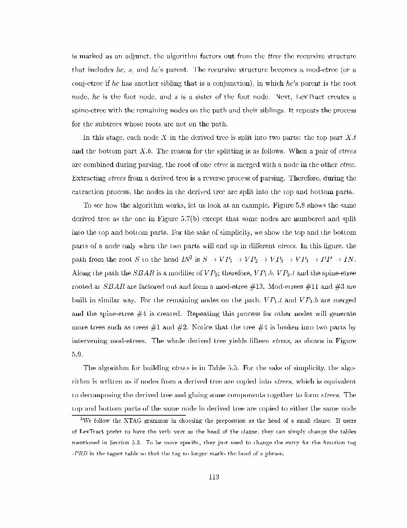
is marked as an adjunct, the algorithm factors out from the ttree the recursive structure
that includes hc, s, and hc's parent. The recursive structure becomes a mod-etree (or a
conj-etree if hc has another sibling that is a conjunction), in which hc's parent is the root
node, hc is the foot node, and s is a sister of the foot node. Next, LexTract creates a
spine-etree with the remaining nodes on the path and their siblings. It repeats the process
for the subtrees whose roots are not on the path.
In this stage, each node X in the derived tree is split into two parts: the top part X:t
and the bottom part X:b. The reason for the splitting is as follows. When a pair of etrees
are combined during parsing, the root of one etree is merged with a node in the other etree.
Extracting etrees from a derived tree is a reverse process of parsing. Therefore, during the
extraction process, the nodes in the derived tree are split into the top and bottom parts.
To see how the algorithm works, let us look at an example. Figure 5.8 shows the same
derived tree as the one in Figure 5.7(b) except that some nodes are numbered and split
into the top and bottom parts. For the sake of simplicity, we show the top and the bottom
parts of a node only when the two parts will end up in di�erent etrees. In this �gure, the
path from the root S to the head IN3 is S ! V P1 ! V P2 ! V P3 ! V P4 ! PP ! IN .
Along the path the SBAR is a modi�er of V P2; therefore, V P1:b, V P2:t and the spine-etree
rooted at SBAR are factored out and form a mod-etree #13. Mod-etrees #11 and #3 are
built in similar way. For the remaining nodes on the path, V P1:t and V P4:b are merged
and the spine-etree #4 is created. Repeating this process for other nodes will generate
more trees such as trees #1 and #2. Notice that the tree #4 is broken into two parts by
intervening mod-etrees. The whole derived tree yields �fteen etrees, as shown in Figure
5.9.
The algorithm for building etrees is in Table 5.5. For the sake of simplicity, the algo-
rithm is written as if nodes from a derived tree are copied into etrees, which is equivalent
to decomposing the derived tree and gluing some components together to form etrees. The
top and bottom parts of the same node in derived tree are copied to either the same node
3We follow the XTAG grammar in choosing the preposition as the head of a small clause. If users
of LexTract prefer to have the verb were as the head of the clause, they can simply change the tables
mentioned in Section 5.3. To be more speci�c, they just need to change the entry for the function tag
-PRD in the tagset table so that the tag no longer marks the head of a phrase.
113

S
NP
NN
Supply VPVPNNS
troubles VBD
IN
on
were
VP
yesterday
RB
NP
VP
worried
SBAR
#1
#2
#3
#4
#11
#13
#4
3.t
3.b
VP4.tVP 4.b
2.b
2.t
1.t
1.bNP
2.t
NP 2.b
NP
VP 1.tVP 1.b
NP 3.bNP 3.t
PP
Figure 5.8: The etree set is a decomposition of the derived tree.
in one etree or two nodes in two distinct etrees. The lines labeled (EC1) and (EC2)
in Table 5.5 are used to handle empty categories, and their usage shall be explained in
Section 5.8.2.
Annotation errors in ttrees will result in linguistically implausible etrees. For example,
in the sentence in Figure 5.7(a), the word yesterday is incorrectly tagged as RB (adverb).
As a result, one of the etrees, #11 in Figure 5.9, is created. The etree is linguistically
implausible because an adverb should not be the head of an NP (noun phrase). In Section
6.1.3, we shall propose two methods for �ltering out implausible etrees.
5.4.3 Uniqueness of decomposition
So far, we have discussed the extraction algorithm used by LexTract. The algorithm takes
three tables with language-speci�c information and a ttree T , and creates (1) a derived
tree T �, and (2) a set Eset of etrees. One advantageous property of ESet is that it is the
only tree set that satis�es all the following conditions:
(C1) Decomposition: The tree set is a decomposition of T �; that is, T � can be generated
by combining the trees in the set via the substitution and adjoining operations.
114
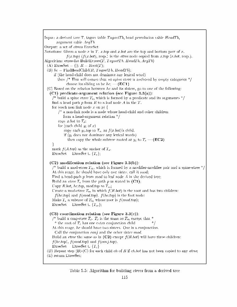
Input: a derived tree T, tagset table TagsetT b, head percolation table HeadTb,argument table ArgTb
Output: a set of etrees EtreeSetNotations: Given a node x in T , x:top and x:bot are the top and bottom part of x.
f(x:top) (f(x:bot), resp.) is the etree node copied from x:top (x:bot, resp.).Algorithm: etree-list BuildEtrees(T , TagsetT b, HeadTb, ArgTb)(A) EtreeSet = fg; R = Root(T );(B) hc = FindHeadChild(R, TagsetT b, HeadTb);
if (the head-child does not dominate any lexical word)then /* This will ensure that no spine etree is anchored by empty categories */
choose its sibling to be hc; | (EC1)(C) Based on the relation between hc and its sisters, go to one of the following:(C1) predicate-argument relation (see Figure 3.3(a)):/* build a spine-etree Ts, which is formed by a predicate and its arguments */�nd a head-path p from R to a leaf node A in the T .for (each non-link node x on p) f
/* a non-link node is a node whose head-child and other childrenform a head-argument relation */
copy x:bot to Ts;for (each child yi of x)
copy each yi:top to Ts, as f(x:bot)'s child.if (yi does not dominate any lexical words)then copy the whole subtree rooted at yi to Ts | (EC2)
gmark f(A:top) as the anchor of Ts.EtreeSet = EtreeSet [ fTsg;
(C2) modi�cation relation (see Figure 3.3(b)):/* build a mod-etree Tm, which is formed by a modi�er-modi�ee pair and a spine-etree */At this stage, hc should have only one sister, call it mod;Find a head-path p from mod to leaf node A in the derived tree;Build an etree Ts from the path p as stated in (C1);Copy R:bot, hc:top, mod:top to Tm;Create a mod-etree Tm in which f(R:bot) is the root and has two children:f(hc:top) and f(mod:top). f(hc:top) is the foot node;
Make Ts a subtree of Tm whose root is f(mod:top);EtreeSet = EtreeSet [ fTmg;
(C3) coordination relation (see Figure 3.3(c)):/* build a conj-etree Tc. Tc is the same as Tm except that ** the root of Tc has one extra conjunction child */
At this stage, hc should have two sisters. One is a conjunction.Call the conjunction conj and the other sister mod.
Build an etree the same as in (C2) except f(R:bot) will have three children:f(hc:top), f(mod:top) and f(conj:top).EtreeSet = EtreeSet [ fTcg
(D) Repeat step (B)-(C) for each child ch of R if ch:bot has not been copied to any etree;(E) return EtreeSet;
Table 5.5: Algorithm for building etrees from a derived tree
115
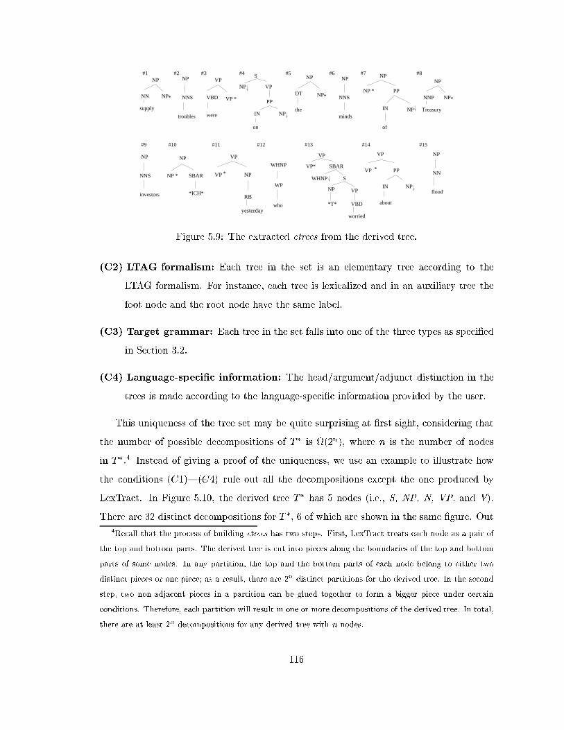
NP
NPNN *
supply
NP
NNS
troubles
NP
the
NP
DT *
NP
NNS
minds
NP
NPNNP *
Treasury
NP
NNS
investors
VP
VP PP
IN NP
about
*
VP
VP NP
RB
yesterday
*
NP
NN
flood
#1 #2 #3 #4 #5 #6 #7 #8
#9 #10 #11 #12 #13 #14 #15
VP
VP* SBAR
S
NP VP
NPIN
PP
on
WHNP
WHNP
who
WP
VP
VBD VP
were
*ICH*
NP
NP * SBAR S
NP VP
VBD*T*
worried
NP
NP
NP PP
of
*
IN
*
Figure 5.9: The extracted etrees from the derived tree.
(C2) LTAG formalism: Each tree in the set is an elementary tree according to the
LTAG formalism. For instance, each tree is lexicalized and in an auxiliary tree the
foot node and the root node have the same label.
(C3) Target grammar: Each tree in the set falls into one of the three types as speci�ed
in Section 3.2.
(C4) Language-speci�c information: The head/argument/adjunct distinction in the
trees is made according to the language-speci�c information provided by the user.
This uniqueness of the tree set may be quite surprising at �rst sight, considering that
the number of possible decompositions of T � is (2n), where n is the number of nodes
in T �.4 Instead of giving a proof of the uniqueness, we use an example to illustrate how
the conditions (C1)|(C4) rule out all the decompositions except the one produced by
LexTract. In Figure 5.10, the derived tree T � has 5 nodes (i.e., S, NP, N, VP, and V).
There are 32 distinct decompositions for T �, 6 of which are shown in the same �gure. Out
4Recall that the process of building etrees has two steps. First, LexTract treats each node as a pair of
the top and bottom parts. The derived tree is cut into pieces along the boundaries of the top and bottom
parts of some nodes. In any partition, the top and the bottom parts of each node belong to either two
distinct pieces or one piece; as a result, there are 2n distinct partitions for the derived tree. In the second
step, two non-adjacent pieces in a partition can be glued together to form a bigger piece under certain
conditions. Therefore, each partition will result in one or more decompositions of the derived tree. In total,
there are at least 2n decompositions for any derived tree with n nodes.
116
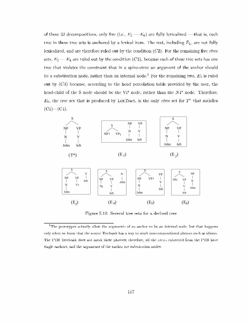
of these 32 decompositions, only �ve (i.e., E2 | E6) are fully lexicalized | that is, each
tree in these tree sets is anchored by a lexical item. The rest, including E1, are not fully
lexicalized, and are therefore ruled out by the condition (C2). For the remaining �ve etree
sets, E2 | E4 are ruled out by the condition (C3), because each of these tree sets has one
tree that violates the constraint that in a spine-etree an argument of the anchor should
be a substitution node, rather than an internal node.5 For the remaining two, E5 is ruled
out by (C4) because, according to the head percolation table provided by the user, the
head-child of the S node should be the VP node, rather than the NP node. Therefore,
E6, the tree set that is produced by LexTract, is the only etree set for T � that satis�es
(C1)|(C4).
N
NP VP
John left
V
S
N
NP VP
John
V
SV
left
E 1 E 2 T*
3E
N
NP VP
John left
V
SNP
N
John
VP
V
left
NP VP
S
NP VP
left
V
S
E 4 E5 E6
N
NP VP
left
V
SN
JohnN
NP VP
John
S
V
left
VP NP
N
John
)
) ( ) )
( )( )
( (
(
( )
Figure 5.10: Several tree sets for a derived tree
5The prototypes actually allow the arguments of an anchor to be an internal node, but that happens
only when we know that the source Treebank has a way to mark non-compositional phrases such as idioms.
The PTB Treebank does not mark these phrases; therefore, all the etrees extracted from the PTB have
single anchors, and the arguments of the anchor are substitution nodes.
117
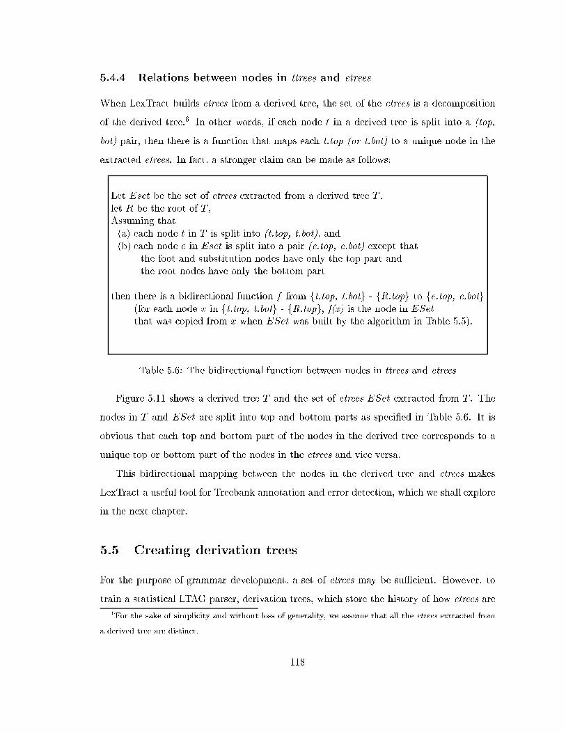
5.4.4 Relations between nodes in ttrees and etrees
When LexTract builds etrees from a derived tree, the set of the etrees is a decomposition
of the derived tree.6 In other words, if each node t in a derived tree is split into a (top,
bot) pair, then there is a function that maps each t.top (or t.bot) to a unique node in the
extracted etrees. In fact, a stronger claim can be made as follows:
Let Eset be the set of etrees extracted from a derived tree T ,let R be the root of T ,Assuming that(a) each node t in T is split into (t.top, t.bot), and(b) each node e in Eset is split into a pair (e.top, e.bot) except that
the foot and substitution nodes have only the top part andthe root nodes have only the bottom part
then there is a bidirectional function f from ft.top, t.botg - fR.topg to fe.top, e.botg(for each node x in ft.top, t.botg - fR.topg, f(x) is the node in ESetthat was copied from x when ESet was built by the algorithm in Table 5.5).
Table 5.6: The bidirectional function between nodes in ttrees and etrees
Figure 5.11 shows a derived tree T and the set of etrees ESet extracted from T . The
nodes in T and ESet are split into top and bottom parts as speci�ed in Table 5.6. It is
obvious that each top and bottom part of the nodes in the derived tree corresponds to a
unique top or bottom part of the nodes in the etrees and vice versa.
This bidirectional mapping between the nodes in the derived tree and etrees makes
LexTract a useful tool for Treebank annotation and error detection, which we shall explore
in the next chapter.
5.5 Creating derivation trees
For the purpose of grammar development, a set of etrees may be suÆcient. However, to
train a statistical LTAG parser, derivation trees, which store the history of how etrees are
6For the sake of simplicity and without loss of generality, we assume that all the etrees extracted from
a derived tree are distinct.
118
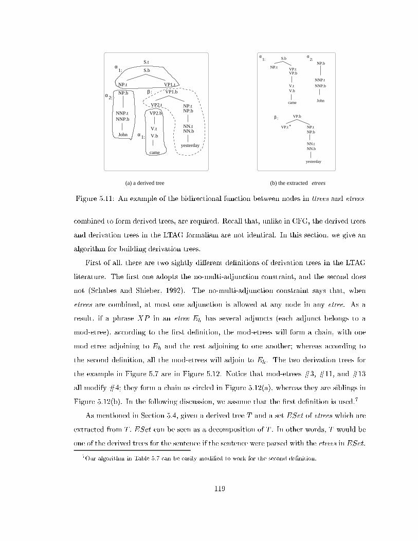
S.t
S.b
NP.t VP1.t
VP1.b
VP2.t
VP2.b
V.t
V.b
came
NP.b
NNP.tNNP.b
John
NP.tNP.b
NN.tNN.b
yesterday
α1:
α2:
α1:
β :
S.b
NP.t VP.tVP.b
V.tV.b
came
α1:
NP.b
NNP.t
NNP.b
John
α2:
VP.t NP.t*
NP.b
NN.tNN.b
yesterday
VP.bβ :
(a) a derived tree (b) the extracted etrees
Figure 5.11: An example of the bidirectional function between nodes in ttrees and etrees
combined to form derived trees, are required. Recall that, unlike in CFG, the derived trees
and derivation trees in the LTAG formalism are not identical. In this section, we give an
algorithm for building derivation trees.
First of all, there are two sightly di�erent de�nitions of derivation trees in the LTAG
literature. The �rst one adopts the no-multi-adjunction constraint, and the second does
not (Schabes and Shieber, 1992). The no-multi-adjunction constraint says that, when
etrees are combined, at most one adjunction is allowed at any node in any etree. As a
result, if a phrase XP in an etree Eh has several adjuncts (each adjunct belongs to a
mod-etree), according to the �rst de�nition, the mod-etrees will form a chain, with one
mod-etree adjoining to Eh and the rest adjoining to one another; whereas according to
the second de�nition, all the mod-etrees will adjoin to Eh. The two derivation trees for
the example in Figure 5.7 are in Figure 5.12. Notice that mod-etrees #3, #11, and #13
all modify #4; they form a chain as circled in Figure 5.12(a), whereas they are siblings in
Figure 5.12(b). In the following discussion, we assume that the �rst de�nition is used.7
As mentioned in Section 5.4, given a derived tree T and a set ESet of etrees which are
extracted from T , ESet can be seen as a decomposition of T . In other words, T would be
one of the derived trees for the sentence if the sentence were parsed with the etrees in ESet.
7Our algorithm in Table 5.7 can be easily modi�ed to work for the second de�nition.
119
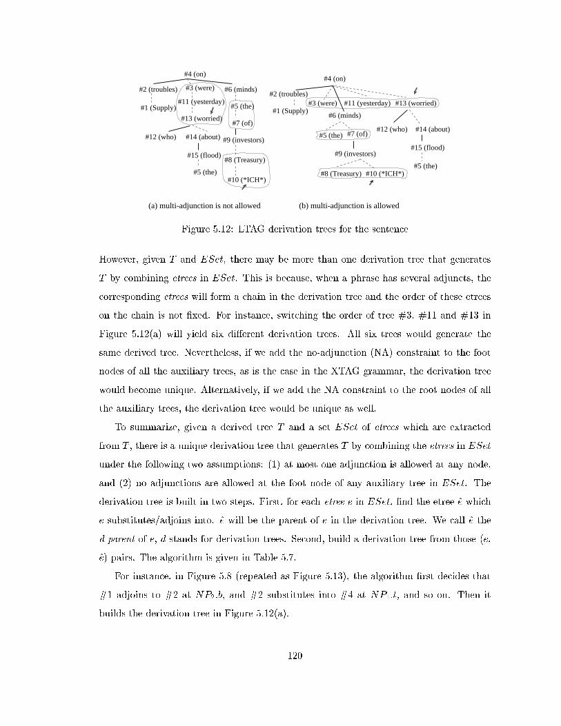
#1 (Supply)
#2 (troubles)
#10 (*ICH*)
#8 (Treasury)
#7 (of)
#5 (the)
#6 (minds)#3 (were)
#4 (on)
#13 (worried)
#12 (who) #14 (about)
#5 (the)
#15 (flood)
#9 (investors)
(a) multi-adjunction is not allowed (b) multi-adjunction is allowed
#4 (on)
#2 (troubles)
#1 (Supply)#13 (worried)#11 (yesterday)
#6 (minds)
#5 (the) #7 (of)
#9 (investors)
#8 (Treasury) #10 (*ICH*)
#12 (who) #14 (about)
#15 (flood)
#5 (the)
#11 (yesterday) #3 (were)
Figure 5.12: LTAG derivation trees for the sentence
However, given T and ESet, there may be more than one derivation tree that generates
T by combining etrees in ESet. This is because, when a phrase has several adjuncts, the
corresponding etrees will form a chain in the derivation tree and the order of these etrees
on the chain is not �xed. For instance, switching the order of tree #3, #11 and #13 in
Figure 5.12(a) will yield six di�erent derivation trees. All six trees would generate the
same derived tree. Nevertheless, if we add the no-adjunction (NA) constraint to the foot
nodes of all the auxiliary trees, as is the case in the XTAG grammar, the derivation tree
would become unique. Alternatively, if we add the NA constraint to the root nodes of all
the auxiliary trees, the derivation tree would be unique as well.
To summarize, given a derived tree T and a set ESet of etrees which are extracted
from T , there is a unique derivation tree that generates T by combining the etrees in ESet
under the following two assumptions: (1) at most one adjunction is allowed at any node,
and (2) no adjunctions are allowed at the foot node of any auxiliary tree in ESet. The
derivation tree is built in two steps. First, for each etree e in ESet, �nd the etree e which
e substitutes/adjoins into. e will be the parent of e in the derivation tree. We call e the
d-parent of e, d stands for derivation trees. Second, build a derivation tree from those (e,
e) pairs. The algorithm is given in Table 5.7.
For instance, in Figure 5.8 (repeated as Figure 5.13), the algorithm �rst decides that
#1 adjoins to #2 at NP2:b, and #2 substitutes into #4 at NP1:t, and so on. Then it
builds the derivation tree in Figure 5.12(a).
120
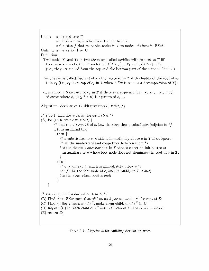
Input: a derived tree T ,an etree set ESet which is extracted from T ,a function f that maps the nodes in T to nodes of etrees in ESet
Output: a derivation tree DDe�nitions:Two nodes Y1 and Y2 in two etrees are called buddies with respect to T i�there exists a node X in T such that f(X:top) = Y1 and f(X:bot) = Y2.(i.e., they are copied from the top and the bottom part of the same node in T )
An etree e1 is called t-parent of another etree e2 in T if the buddy of the root of e2is in e1 (i.e., e1 is on top of e2 in T when ESet is seen as a decomposition of T ).
ex is called a t-ancestor of ey in T if there is a sequence (e0 = ex; e1; :::; en = ey)of etrees where ei (0 � i < n) is t-parent of ei+1.
Algorithm: deriv-tree* BuildDerivTree(T , ESet, f)
/* step 1: �nd the d-parent for each etree */(A) for (each etree e in ESet) f
/* �nd the d-parent e of e, i.e., the etree that e substitutes/adjoins to */if (e is an initial tree)then f/* e substitutes to e, which is immediately above e in T if we ignore* all the mod-etrees and conj-etrees between them */e is the closest t-ancestor of e in T that is either an initial tree oran auxiliary tree whose foot node does not dominate the root of e in T .g
else f/* e adjoins to e, which is immediately below e */Let fn be the foot node of e, and its buddy in T is bud;e is the etree whose root is bud;g
g
/* step 2: build the derivation tree D */(B) Find eR 2 ESet such that eR has no d-parent, make eR the root of D.(C) Find all the d-children of eR, make them children of eR in D.(D) Repeat (C) for each child of eR until D includes all the etrees in ESet;(E) return D;
Table 5.7: Algorithm for building derivation trees
121
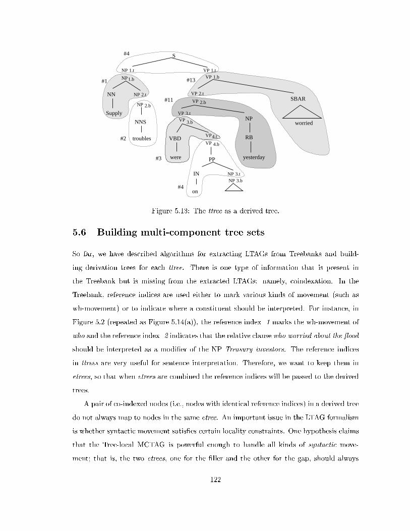
S
NP
NN
Supply VPVPNNS
troubles VBD
IN
on
were
VP
yesterday
RB
NP
VP
worried
SBAR
#1
#2
#3
#4
#11
#13
#4
3.t
3.b
VP4.tVP 4.b
2.b
2.t
1.t
1.bNP
2.t
NP 2.b
NP
VP 1.tVP 1.b
NP 3.bNP 3.t
PP
Figure 5.13: The ttree as a derived tree.
5.6 Building multi-component tree sets
So far, we have described algorithms for extracting LTAGs from Treebanks and build-
ing derivation trees for each ttree. There is one type of information that is present in
the Treebank but is missing from the extracted LTAGs: namely, coindexation. In the
Treebank, reference indices are used either to mark various kinds of movement (such as
wh-movement) or to indicate where a constituent should be interpreted. For instance, in
Figure 5.2 (repeated as Figure 5.14(a)), the reference index -1 marks the wh-movement of
who and the reference index -2 indicates that the relative clause who worried about the ood
should be interpreted as a modi�er of the NP Treasury investors. The reference indices
in ttrees are very useful for sentence interpretation. Therefore, we want to keep them in
etrees, so that when etrees are combined the reference indices will be passed to the derived
trees.
A pair of co-indexed nodes (i.e., nodes with identical reference indices) in a derived tree
do not always map to nodes in the same etree. An important issue in the LTAG formalism
is whether syntactic movement satis�es certain locality constraints. One hypothesis claims
that the Tree-local MCTAG is powerful enough to handle all kinds of syntactic move-
ment; that is, the two etrees, one for the �ller and the other for the gap, should always
122
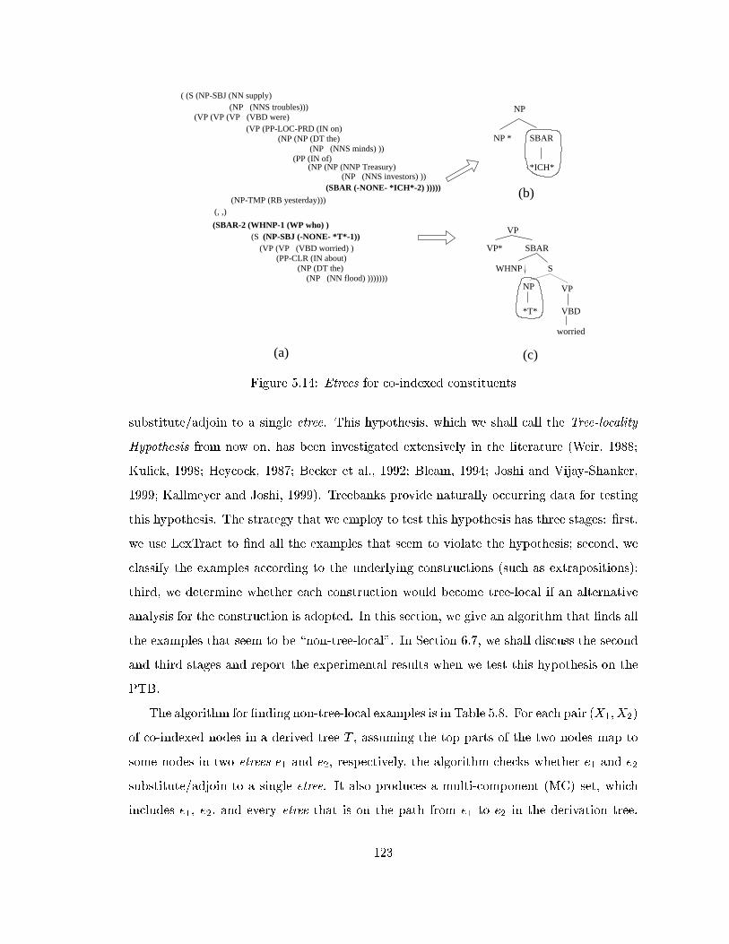
( (S (NP-SBJ (NN supply)(NP (NNS troubles)))
(VP (VP (VP (VBD were)(VP (PP-LOC-PRD (IN on)
(NP (NP (DT the)(NP (NNS minds) ))
(PP (IN of)(NP (NP (NNP Treasury)
(NP-TMP (RB yesterday)))(, ,)
(SBAR-2 (WHNP-1 (WP who) )
(VP (VP (VBD worried) )(PP-CLR (IN about)
(NP (DT the) (NP (NN flood) )))))))
(S (NP-SBJ (-NONE- *T*-1))
(NP (NNS investors) ))(SBAR (-NONE- *ICH*-2) )))))
(a)
(b)
(c)
VP
VP* SBAR
WHNP S
NP VP
VBD*T*
worried
*ICH*
NP
NP * SBAR
Figure 5.14: Etrees for co-indexed constituents
substitute/adjoin to a single etree. This hypothesis, which we shall call the Tree-locality
Hypothesis from now on, has been investigated extensively in the literature (Weir, 1988;
Kulick, 1998; Heycock, 1987; Becker et al., 1992; Bleam, 1994; Joshi and Vijay-Shanker,
1999; Kallmeyer and Joshi, 1999). Treebanks provide naturally occurring data for testing
this hypothesis. The strategy that we employ to test this hypothesis has three stages: �rst,
we use LexTract to �nd all the examples that seem to violate the hypothesis; second, we
classify the examples according to the underlying constructions (such as extrapositions);
third, we determine whether each construction would become tree-local if an alternative
analysis for the construction is adopted. In this section, we give an algorithm that �nds all
the examples that seem to be \non-tree-local". In Section 6.7, we shall discuss the second
and third stages and report the experimental results when we test this hypothesis on the
PTB.
The algorithm for �nding non-tree-local examples is in Table 5.8. For each pair (X1;X2)
of co-indexed nodes in a derived tree T , assuming the top parts of the two nodes map to
some nodes in two etrees e1 and e2, respectively, the algorithm checks whether e1 and e2
substitute/adjoin to a single etree. It also produces a multi-component (MC) set, which
includes e1, e2, and every etree that is on the path from e1 to e2 in the derivation tree.
123

Figure 5.15 shows three scenarios of a derivation tree. In (a), e1 and e2 are identical; that
is, the co-indexed nodes appear in the same etree. In (b), e1 and e2 substitute/adjoin
to the same etree ea. In (c), e1 and e2 do not substitute/adjoin to the same etree. The
relation between X1 and X2 is tree-local in (a) and (b), but it is not tree-local in (c).
X .top2
1X .top
1X .topX .top
2
1X .top X .top2
e 1 e 2
e a
e 1 e 2
e ae = e
21
(c) not tree-local(b) tree-local(a) within one tree
Figure 5.15: The coindexation between two nodes may or may not be tree-local
In Figure 5.14(a), theWHNP-1 and *T*-1 map to nodes in the same etree in (c), so the
movement from *T*-1 to WHNP-1 can be handled by the Tree-local MCTAG. In contrast,
as shown in Figures 5.16 and 5.17, the etrees for *ICH*-2 and SBAR-2 (i.e., #10 and
#13) do not adjoin to a single etree; therefore, the \movement" from *ICH*-2 to SBAR-2
cannot be handled by the Tree-local MCTAG according to the current annotation in the
ttree.8
8In (Xia and Bleam, 2000), we argue that this type of example (called NP-extraposition) is not syntactic
movement; therefore, it is not a counter-example to the Tree-locality Hypothesis.
#12 (who) #14 (about)
#15 (flood)
#11 (yesterday)#2 (troubles)
#1 (Supply)#3 (were)
#5 (the)
#8 (Treasury) #10 (*ICH*)
#9 (investors)
#7 (of)
#6 (minds)
#4 (on)
#13 (worried)
#5 (the)
Figure 5.16: The LTAG derivation tree for the sentence when multi-adjunction is allowed
124
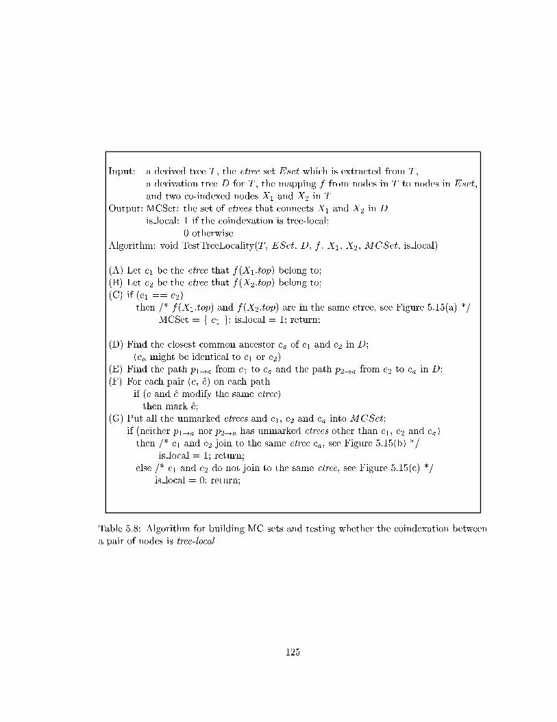
Input: a derived tree T , the etree set Eset which is extracted from T ,a derivation tree D for T , the mapping f from nodes in T to nodes in Eset,and two co-indexed nodes X1 and X2 in T
Output: MCSet: the set of etrees that connects X1 and X2 in Dis local: 1 if the coindexation is tree-local;
0 otherwiseAlgorithm: void TestTreeLocality(T , ESet, D, f , X1, X2, MCSet, is local)
(A) Let e1 be the etree that f(X1:top) belong to;(B) Let e2 be the etree that f(X2:top) belong to;(C) if (e1 == e2)
then /* f(X1:top) and f(X2:top) are in the same etree, see Figure 5.15(a) */MCSet = f e1 g; is local = 1; return;
(D) Find the closest common ancestor ea of e1 and e2 in D;(ea might be identical to e1 or e2)
(E) Find the path p1!a from e1 to ea and the path p2!a from e2 to ea in D;(F) For each pair (e, e) on each path
if (e and e modify the same etree)then mark e;
(G) Put all the unmarked etrees and e1, e2 and ea into MCSet;if (neither p1!a nor p2!a has unmarked etrees other than e1, e2 and ea)then /* e1 and e2 join to the same etree ea, see Figure 5.15(b) */
is local = 1; return;else /* e1 and e2 do not join to the same etree, see Figure 5.15(c) */
is local = 0; return;
Table 5.8: Algorithm for building MC sets and testing whether the coindexation betweena pair of nodes is tree-local
125

NP
NNS
investors
α3:
β1:
NP
NP
NP PP
of
*
IN
NP
NNS
minds
α2:
α 1: VP
IN
on
NP
PP
S
NP
*
i
NP
NP SBAR
ε
β2:
*
β3:
VP SBAR i
VP
NP
worried
VBD
VP
SWHNP
ε
Figure 5.17: The etrees that connect the ones for *ICH*-2 and SBAR-2 in the derivationtree.
5.7 Building context-free rules and sub-templates
LexTract is designed to extract LTAGs, but simply reading context-free rules o� the tem-
plates in an extracted LTAG will yield a CFG. For example, the template in Figure 5.18(a)
will yield two context-free rules in 5.18(b).
S
NP VP
NPVBD@
(1) S -> NP VP
(2) VP -> VBD NP
(a) a template (b) CFG rules derived from (a)
Figure 5.18: The context-free rules derived from a template
We can also obtain subcategorization information from a template by decomposing
the template into a set of sub-templates as follows: a spine-etree template is decomposed
into a subcategorization chain and a subcategorization frame; a mod-etree template is
126
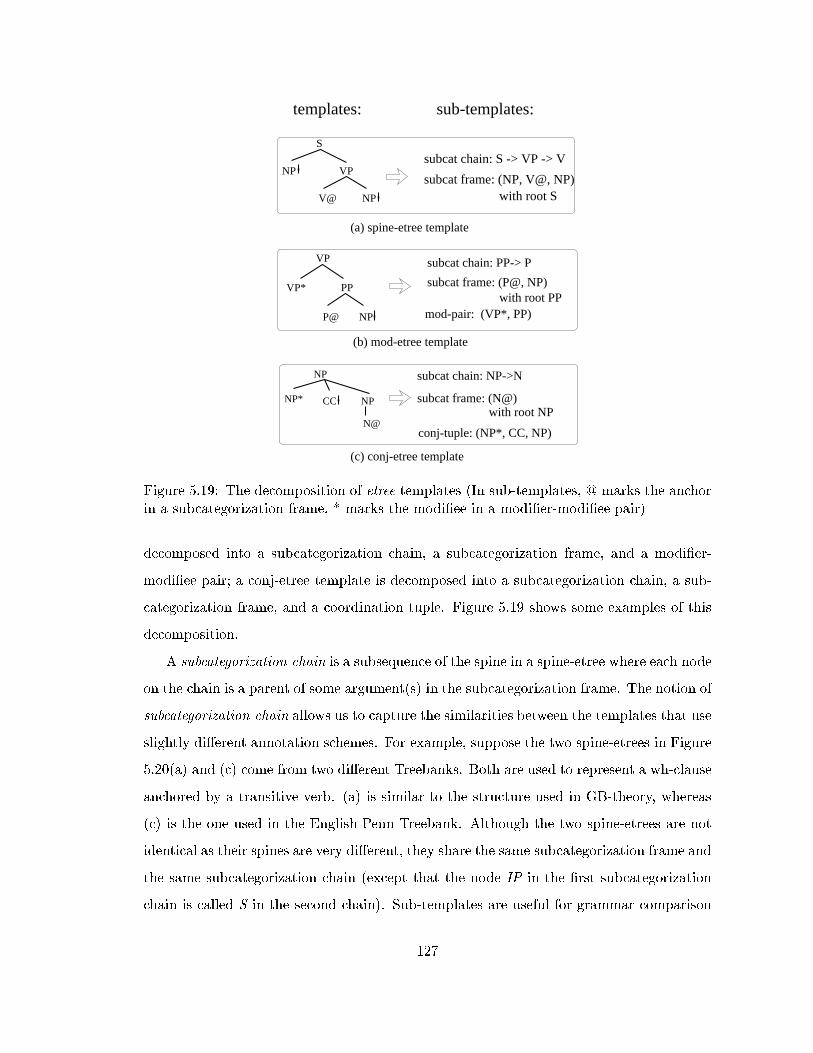
VP
VP* PP
P@ NP
NP
NP* CC NP
N@
sub-templates:templates:
(a) spine-etree template
(b) mod-etree template
S
NP VP
NPV@
subcat frame: (NP, V@, NP)
subcat chain: S -> VP -> V
with root S
mod-pair: (VP*, PP)
subcat frame: (P@, NP)
subcat chain: PP-> P
with root PP
subcat chain: NP->N
subcat frame: (N@)with root NP
(c) conj-etree template
conj-tuple: (NP*, CC, NP)
Figure 5.19: The decomposition of etree templates (In sub-templates, @ marks the anchorin a subcategorization frame, * marks the modi�ee in a modi�er-modi�ee pair)
decomposed into a subcategorization chain, a subcategorization frame, and a modi�er-
modi�ee pair; a conj-etree template is decomposed into a subcategorization chain, a sub-
categorization frame, and a coordination tuple. Figure 5.19 shows some examples of this
decomposition.
A subcategorization chain is a subsequence of the spine in a spine-etree where each node
on the chain is a parent of some argument(s) in the subcategorization frame. The notion of
subcategorization chain allows us to capture the similarities between the templates that use
slightly di�erent annotation schemes. For example, suppose the two spine-etrees in Figure
5.20(a) and (c) come from two di�erent Treebanks. Both are used to represent a wh-clause
anchored by a transitive verb. (a) is similar to the structure used in GB-theory, whereas
(c) is the one used in the English Penn Treebank. Although the two spine-etrees are not
identical as their spines are very di�erent, they share the same subcategorization frame and
the same subcategorization chain (except that the node IP in the �rst subcategorization
chain is called S in the second chain). Sub-templates are useful for grammar comparison
127

spine: CP -> C’ -> IP -> I’ -> VP -> V
subcat chain: IP -> VP -> V
subcat frame: (NP, V@, NP)
spine: SBAR -> S -> VP -> V
subcat chain: S -> VP -> V
subcat frame: (NP, V@, NP)
(a)
(c)
(b)
(d)
SBAR
WHNP
NP VP
V@ NP
S
COMP
NP
IP
CP
WHNP
INFL VP
V@ NP
I’
C’
Figure 5.20: Spines, subcategorization chains, and subcategorization frames
and language comparison (See Sections 6.2 and 6.3).
5.8 Some special cases
In this section, we discuss four cases that require special consideration from LexTract.
5.8.1 Coordination
In this chapter, we de�ne a conj-etree as an etree with the conjunction represented as a
substitution node, one XP as the foot node and the other XP expanded (e.g., �1 in Figure
5.21). An alternative is to treat the conjunction as the anchor, one XP as the foot, and
the other XP as a substitution node (e.g., �2 in Figure 5.21). Figure 5.21 shows how these
two approaches handle a VP coordination in the sentence John bought a book and has read
it four times. In the �rst approach, the second verb read anchors the conj-etree �1, and
the singleton etree �1 substitutes into the CC node in �1. In the second approach, the
conj-etree �2 is anchored by the conjunction, and the etree �2 substitutes into the VP node
in �2. In either approach, the conj-etree adjoins to the etree �3.
Currently, we choose the �rst approach for two reasons. First, it can easily capture the
128
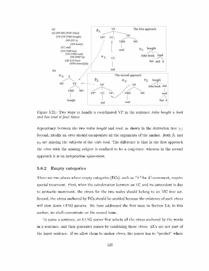
read
(QP (CD four)
S
NP VP
VBD NP
bought
and
CC
(NNS times)))))))
(b)
VP
VP
VBD NP
read
CCVP*
VP* CC VP
VP
and
(a)
VBD NP
VP
(NP (PRP it))(VP (VBD read)
(NN book))
(NP (DT a)
(VP (VP (VBD bought)
((S (NP-SBJ (NNP John))
(CC and)1:γ
1:
1:β
The second approach
The first approach
γβ2: 2:α2:
α
(VP (VBP has)
read
and it
John book
bought
has
John bookand
read
bought
ithas
α 3:
Figure 5.21: Two ways to handle a coordinated VP in the sentence John bought a bookand has read it four times
dependency between the two verbs bought and read, as shown in the derivation tree 1;
Second, ideally an etree should encapsulate all the arguments of the anchor. Both �1 and
�2 are missing the subjects of the verb read. The di�erence is that in the �rst approach
the etree with the missing subject is con�ned to be a conj-etree, whereas in the second
approach it is an independent spine-etree.
5.8.2 Empty categories
There are two places where empty categories (ECs), such as *T* for A'-movement, require
special treatment. First, when the coindexation between an EC and its antecedent is due
to syntactic movement, the etrees for the two nodes should belong to an MC tree set.
Second, the etrees anchored by ECs should be avoided because the existence of such etrees
will slow down LTAG parsers. We have addressed the �rst issue in Section 5.6, in this
section, we shall concentrate on the second issue.
To parse a sentence, an LTAG parser �rst selects all the etrees anchored by the words
in a sentence, and then generates parses by combining these etrees. ECs are not part of
the input sentence. If we allow them to anchor etrees, the parser has to \predict" where
129
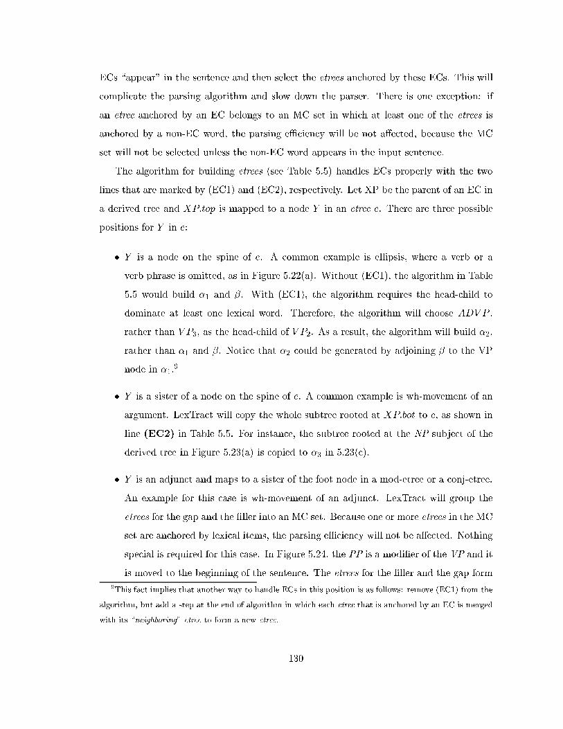
ECs \appear" in the sentence and then select the etrees anchored by these ECs. This will
complicate the parsing algorithm and slow down the parser. There is one exception: if
an etree anchored by an EC belongs to an MC set in which at least one of the etrees is
anchored by a non-EC word, the parsing eÆciency will be not a�ected, because the MC
set will not be selected unless the non-EC word appears in the input sentence.
The algorithm for building etrees (see Table 5.5) handles ECs properly with the two
lines that are marked by (EC1) and (EC2), respectively. Let XP be the parent of an EC in
a derived tree and XP:top is mapped to a node Y in an etree e. There are three possible
positions for Y in e:
� Y is a node on the spine of e. A common example is ellipsis, where a verb or a
verb phrase is omitted, as in Figure 5.22(a). Without (EC1), the algorithm in Table
5.5 would build �1 and �. With (EC1), the algorithm requires the head-child to
dominate at least one lexical word. Therefore, the algorithm will choose ADV P ,
rather than V P3, as the head-child of V P2. As a result, the algorithm will build �2,
rather than �1 and �. Notice that �2 could be generated by adjoining � to the VP
node in �1.9
� Y is a sister of a node on the spine of e. A common example is wh-movement of an
argument. LexTract will copy the whole subtree rooted at XP:bot to e, as shown in
line (EC2) in Table 5.5. For instance, the subtree rooted at the NP subject of the
derived tree in Figure 5.23(a) is copied to �3 in 5.23(c).
� Y is an adjunct and maps to a sister of the foot node in a mod-etree or a conj-etree.
An example for this case is wh-movement of an adjunct. LexTract will group the
etrees for the gap and the �ller into an MC set. Because one or more etrees in the MC
set are anchored by lexical items, the parsing eÆciency will not be a�ected. Nothing
special is required for this case. In Figure 5.24, the PP is a modi�er of the VP and it
is moved to the beginning of the sentence. The etrees for the �ller and the gap form
9This fact implies that another way to handle ECs in this position is as follows: remove (EC1) from the
algorithm, but add a step at the end of algorithm in which each etree that is anchored by an EC is merged
with its \neighboring" etree to form a new etree.
130

NP VP
*?*
Sα1: VP
VP* ADVP
RB
too
β:α2: S
NP VP
too*?*
VP ADVP
RB
NP
John VBD
did
VP
VP ADVP
RB
too
VP
S
1
2
3
*?*
without (EC1)(b) (c) with (EC1)
(a) a ttree
Figure 5.22: Handling a sentence with ellipsis: fMary came yesterday,g John did too
an MC set, and both etrees adjoin to �1.
5.8.3 Punctuation marks
Punctuation marks help humans to comprehend sentences. They can help NLP tools as
well if used appropriately. In the XTAG grammar, there are 47 templates that contain
punctuation marks. Doran (1998) discussed all of the templates in detail. She divided
punctuation marks into three classes: balanced, structural, and terminal. The balanced
punctuation marks are quotes and parentheses; structural marks are commas, dashes,
semi-colons and colons; and terminals are periods, exclamation points and question marks.
Figure 5.25 shows four etrees with punctuation marks: �1 is an etree for non-peripheral
NP appositive, �2 is for a sentence such as \John will come, I think", �3 and �4 are for
balanced and terminal punctuation marks, respectively.10
This approach is appealing when the grammar is built by hand. However, automatically
extracting those etrees from Treebanks is not trivial. For example, in Figure 5.25, the
comma anchors �1, but it is a substitution node in �2. Given a sentence with a comma,
it is not clear how an extraction tool can decide whether the comma should anchor an
10�1 and �2 in Figure 5.25 come from (Doran, 2000).
131

WHNPi
SBAR
S
NP
ε
i VP
V
WP
who
bought the books
NP
NP
ε
SBARα α
1: 2:
SWHNP
NP VP
V NP
bought
WHNP
SBAR
S
VP
NPV
bought
NP
ε
α 3:
(b) without (EC2) (c) with (EC2)
ttree(a) a
Figure 5.23: Handling a sentence with wh-movement from an argument position
NP VP
V
stay
S
β β2:
α 1:
1:
(b) extracted (a) a
S
PP iS
V
did
S
NP
you
VP
VP
V
stay
PP
ε
hotelat which
i
S
PP S*
P NP
at
VP
PPVP* i
ε
i
ttree etrees
Figure 5.24: Handling a sentence with wh-movement from an adjunct position
etree as in �1, and it should be a substitution node as in �2. Another problem is that the
usage of punctuation marks in naturally occurring data is very complicated. For instance,
balanced punctuation marks such as quotation marks are supposed to appear in pairs and
enclose a constituent in a ttree, but they are often not annotated that way in a Treebank
for various reasons. For example, the sentence He said , \S1 . S2 . S3 ." (Si's are clauses)
is broken into three ttrees in the PTB, according to the positions of three periods. The
left quotation mark belongs to the �rst ttree and the right quotation mark belongs to the
third ttree. Another example is in Figure 5.26, where the left quotation mark is a child of
132
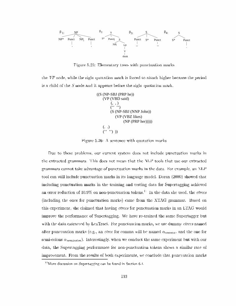
S
S*Punct Punct
‘‘ ’’
β3:
S* Punct
.
Sβ4:
S*
S
Punct S
VPNP
β2:
V
think
NP
NP* Punct NP Punct
, ,
β 1:
Figure 5.25: Elementary trees with punctuation marks
the VP node, while the right quotation mark is forced to attach higher because the period
is a child of the S node and it appears before the right quotation mark.
((S (NP-SBJ (PRP he)) (VP (VBD said) (, , )
(‘‘ ‘‘)(S (NP-SBJ (NNP John))
(VP (VBZ likes)(NP (PRP her)))))
(. .)(’’ ’’) ))
Figure 5.26: A sentence with quotation marks
Due to these problems, our current system does not include punctuation marks in
the extracted grammars. This does not mean that the NLP tools that use our extracted
grammars cannot take advantage of punctuation marks in the data. For example, an NLP
tool can still include punctuation marks in its language model. Doran (2000) showed that
including punctuation marks in the training and testing data for Supertagging achieved
an error reduction of 10.9% on non-punctuation tokens.11 In the data she used, the etrees
(including the ones for punctuation marks) came from the XTAG grammar. Based on
this experiment, she claimed that having etrees for punctuation marks in an LTAG would
improve the performance of Supertagging. We have re-trained the same Supertagger but
with the data extracted by LexTract. For punctuation marks, we use dummy etrees named
after punctuation marks (e.g., an etree for comma will be named �comma, and the one for
semi-colons �semicolon). Interestingly, when we conduct the same experiment but with our
data, the Supertagging performance for non-punctuation tokens shows a similar rate of
improvement. From the results of both experiments, we conclude that punctuation marks
11More discussion on Supertagging can be found in Section 6.4.
133

are de�nitely useful for NLP tools such as a Supertagger, but there is more than one way
to take them into account: for example, they can be included in the etrees of an LTAG, or
they can be part of a language model, or both. Which approach works the best depends
on the application and the particular models used by the NLP tools.
5.8.4 Predicative auxiliary trees
Predicative auxiliary trees, such as the one in Figure 5.27(c) for the verb believe, represent
the head-argument relation, and therefore are spine-etrees. Nevertheless, the structures of
the trees are recursive in that the root and one leaf node have the same label. Following
(Kroch and Joshi, 1985; Kroch, 1989), the XTAG grammar treats this type of tree as an
auxiliary tree to account for long-distance movement such as the sentence what does Mary
think Mike believes John likes (see Section 2.3).
(NP (NP (DT the)
(NN person))
(SBAR (WHNP-1 (WP who))
(VP (VBD believed)(SBAR (-NONE- 0)
(VP (VBD bought)(NP (DT the) (NN book)))))))))
(NP-SBJ (NNP Mary))
(NP-SBJ (-NONE- *T*-1))
(S
(S
(c)(b)(a)
believed
VBD
VP
S
SBAR
NP
WHNP
SBAR*
NP
NP*
VP
VBD NP
S
SBAR
0
bought
NP
*T*
Figure 5.27: An example in which the etree for believed should be a predicative auxiliarytree: the person who Mary believed bought the book
Several things are worth noting:
� When there is no long-distance movement, it does not make much di�erence whether
such an etree is treated as an auxiliary tree or not. For instance, to parse the sentence
Mary believed John would come, either G1 or G2 in Figure 5.28 will work although
the order between come and believed is ipped in the derivation trees. For more
discussion on this topic, see (Joshi and Vijay-Shanker, 1999).
� The shape of the etree alone cannot determine whether it should be an initial tree
or an auxiliary tree. For instance, the etree in Figure 5.29 comes from the XTAG
grammar and it is used to handle gerund phrases such as Mary having a child in the
sentence Nobody heard of Mary having a child. The root of the etree is an NP because
134

S
come
NP VP
VB
S
come
NP VP
VB
3 (come)
1 (believed)
G1
G2
NP VP
S*
believed
S
NP VP
S
believed
S
VBD
VBD
α
β
1: α2:
α1: 3:
α
2(come)α
1 (believed)
α
β
γ2:
γ1:
Figure 5.28: Two alternatives for the verb believed when there is no long-distance movement
the gerund phrase has the same distribution as other NPs. The etree is treated as
an initial tree, although the object of the anchor has the same syntactic tag as the
root.
NP VP
NP
having
VBG NP
Figure 5.29: The etree for gerund in the XTAG grammar
� In some cases, the positions of ECs in the ttrees would determine whether an etree
should be a predicative auxiliary tree. For example, the ttree for the noun phrase
\the person who Mary believed bought the book" in Figure 5.27(a) looks identical to
the ttree for the noun phrase \the person who believed Mary bought the book" in
Figure 5.30(a) except that the positions for Mary and *T* are swapped. But the
etrees needed to parse the two sentences are very di�erent, as in (b) and (c) of Figure
135

5.27 and Figure 5.30. Only the ttree in Figure 5.27(a) requires the etree for the word
believed to be a predicative auxiliary tree.12
NP*
NP
(b)
believed
*T* VBD
VP
S
SBAR
NP
WHNP
SBAR
(NP (NP (DT the)
(NN person))
(WHNP-1 (WP who))
(VP (VBD believed)(SBAR (-NONE- 0)
(VP (VBD bought)(NP (DT the) (NN book)))))))))
(NP-SBJ (-NONE- *T*-1))(S
(S (NP-SBJ (NNP Mary))
(SBAR
(a) (c)
VP
VBD
S
SBAR
0
bought
NP
NP
Figure 5.30: An example in which the etree for believed should not be a predicative auxiliarytree: the person who believed Mary bought the book
To conclude, it is not true that every spine-etree whose root and a leaf node have the
same syntactic tag should be treated as a predicative auxiliary tree. We shall leave the
task of detecting predicative auxiliary trees for future study.
5.9 Comparison with other work
In this section, we compare LexTract with other extraction algorithms for CFGs and
LTAGs proposed in the literature.
5.9.1 CFG extraction algorithms
Many systems that use Treebank context-free grammars simply read context-free rules o�
the phrase structures in Treebanks. Because the phrase structures in the source Treebanks
are partially at, the resulting grammars are very large. One of the most recent works that
address this problem is (Krotov et al., 1998), which gave an algorithm that reduces the size
of the derived grammar by eliminating redundant rules. A rule is redundant if it can be
\parsed" (in the familiar sense of context-free parsing) using other rules of the grammar.
The algorithm checks each rule in the grammar in turn and removes the redundant rules
from the grammar.13 The rules that remain when all rules have been checked constitute
12The etree in Figure 5.30(b) is an auxiliary tree, but it is not a predicative auxiliary tree.13For example, given a grammar that has the following rules: (1) VP ! VB NP PP, (2) VP ! VB NP,
and (3) NP ! NP PP, the algorithm would remove rule (1) because rule (1) can be parsed by rules (2)
136
the compacted grammar. The compact grammar for the PTB has 1122 context-free rules,
and the recall and precision of a CFG parser with the compact grammar are 30.93% and
19.18% respectively, in contrast to 70.78% and 77.66% of the same parser with the full
grammar, which has 15,421 context-free rules.
Krotov's method di�ers dramatically from LexTract in several ways. First, it does not
use the notion of head and it does not distinguish adjuncts and arguments. Second, the
compacting process may result in di�erent grammars depending on the order in which the
rules in the full grammar are checked. To maintain the order-independence, their algorithm
removed all unary and epsilon rules by collapsing them with the sister nodes. Because of
frequent occurrences of empty categories and unary rules in the Treebank, we suspect that
this practice will make the resulting grammars less intuitive and it might also contribute
to the low parsing accuracy when the compact grammar was used. Third, the growth of
their grammar is non-monotonic in that, as the corpus grows, the size of the grammar may
actually decrease because the new rules in the grammar may cause the existing rules to
become redundant and get eliminated. Although the size of the compact grammar might
approach a limit eventually in their experiment, it is not clear how stable the grammar
really is, considering the existence of annotation errors in the Treebank. For example, it is
possible that a few bad rules (e.g. fX ) X ZPg, where ZP can be any syntactic label) can
ruin the whole grammar because they make many good rules become redundant and get
eliminated. They mentioned in their paper that they developed a linguistic compaction
algorithm that could retain redundant but linguistically valid rules, and they gave the sizes
of two grammars built by this new algorithm. Unfortunately, the description is too sketchy
for us to determine exactly how that algorithm works.
In contrast, LexTract uses the notion of head and it distinguishes arguments from
adjuncts. The CFG produced by LexTract is order-independent, and it allows unary
rules and epsilon rules. In addition, the growth of the grammar is monotonic, and the
existence of bad rules would not a�ect the good rules. As for the number of context-free
rules, the CFG built by LexTract from the PTB has 1524 rules (see Section 6.1), whereas
in Krotov's approach, the compact grammar has 1122 rules and the two linguistically
and (3).
137

compact grammars have 4820 and 6417 rules, respectively.14
5.9.2 LTAG extraction algorithms
In addition to LexTract, there are two systems that extract LTAGs from Treebanks.
Neumann's lexicalized tree grammars
Neumann (1998) describes an extraction algorithm and tests it on the PTB and a German
Treebank called Negra (Skut et al., 1997). There are several similarities between his
approach and LexTract. First, both approaches adopt notions of head and use a head
percolation table to identify the head-child at each level. Second, both decompose the
ttrees from the top downwards such that the subtrees rooted by non-head children are cut
o� and the cutting point is marked for substitution. The main di�erence between the two
is that Neumann's system does not distinguish arguments from adjuncts, and therefore it
does not factor out the majority of recursive structures with adjuncts. As a result, only
7.97% of the templates in his grammar are auxiliary trees, and the size of his grammar
is much larger than ours: his system extracts 11,979 templates from three sections of
the PTB (i.e., Sections 02-04), whereas LexTract extracts 6926 templates from the whole
corpus (i.e., Sections 00-24). It is also not clear from his paper how he treats conjunctions,
empty categories and coindexation; therefore, we cannot compare these two approaches on
these issues.
Chen & Vijay-shanker's approach
Chen & Vijay-shanker's method (2000) is similar to LexTract in that both use a head
percolation table to �nd the head and both distinguish arguments from adjuncts. Never-
theless, there are several di�erences.
The two systems di�er in their overall architectures. When we designed LexTract, we
explicitly de�ned three prototypes of elementary trees in the target grammars. The pro-
totypes are language independent and every etree built by LexTract falls into one of three
14Unfortunately, we don't have access to the CFG parser they used; therefore, we cannot compare our
grammar with their grammars with respect to the precision and recall rates of the parser.
138
prototypes. Given a Treebank and three tables containing language-speci�c information,
for each phrase structure (ttree) in the Treebank, LexTract �rst explicitly creates a derived
tree. It then decomposes the derived tree into a set of etrees. The bidirectional mapping
between the nodes in this derived tree and the etrees makes LexTract a useful tool for
Treebank annotation and error detection (see Section 6.6). LexTract also explicitly builds
a derivation tree and an MC set. Chen & Vijay-shanker's system does not explicitly de�ne
the prototypes of elementary trees. It does not create a derived tree; therefore, there are
no one-to-one mappings between the nodes in a ttree and the nodes in the extracted etrees.
The system does not build derivation trees and MC sets, either.
The two systems also di�er in their algorithms for making argument/adjunct distinc-
tions. Chen & Vijay-shanker's system uses a two-step procedure to determine whether a
node sist is an argument of the head hc. The �rst step considers the syntactic tags and
function tags of sist and its parent. Exactly this information is used as an index into a
manually constructed table. An example of an entry in this table is \if the current node
is PP-DIR and the parent node is VP, then assign adjunct to the current node". If the
index is not found in the table, then the second step of the following procedure is invoked:
� Nonterminal PRN is an adjunct.
� Nonterminal with semantic tags NOM, DTV, LGS, PRD, PUT, SBJ are comple-
ments.
� Nonterminals with semantic tags ADV, VOC, LOC, PRP are adjuncts.
� If none of the other conditions apply, the nonterminal is an adjunct.
In LexTract, the argument/adjunct distinction is made in two steps as well. In the
�rst step, LexTract checks the function tags of sist, which corresponds to the second step
in Chen and Vijay-shanker's system. The di�erence is that, rather than using a �xed
procedure, LexTract allows its users to specify in the tagset table their treatments for the
function tags. For instance, if the users include the entry (PRD HEAD) in the tagset
table, LexTract will treat every phrase with the -PRD (predicate) tag as a head-child.
If the users replace the entry with (PRD ARGUMENT), LexTract will then treat these
139
phrases as arguments. If sist does not have a function tag with which LexTract can decide
the type of the phrase in the �rst step, LexTract invokes a second step, which determines
the type of sist according to the entry for the head sibling hc in the argument table. Recall
that the argument table speci�es not only the possible tags of hc's arguments, but also
the maximal numbers of arguments to the left or the right of hc. In contrast, the �rst step
of Chen & Vijay-shanker's system considers the tags of sist and sist's parent. We believe
that the tag of hc is a better indicator of the type of sist than is the tag of sist's parent,
and the argument table is more informative than the manually constructed table in their
system.
These two systems also di�er in their treatments for coordinations, punctuation marks,
and so forth. Another way to compare these systems is to evaluate the performances of
a common NLP tool that is trained by the data produced by the systems. One of such
tools is Srinivas's Supertagger. In Section 6.4, we shall report the performances of the
Supertagger with the data produced by these two systems.
5.10 Summary
In this chapter, we have outlined a system named LexTract, which takes a Treebank
and language-speci�c information and produces grammars (LTAGs and CFGs), derivation
trees, and MC sets. LexTract has several advantageous properties. First, it takes very
little human e�ort to build three tables (i.e., the tagset table, the head percolation table,
and the argument table). Once the tables are ready, LexTract can extract grammars from
Treebank in little time. Because LexTract does not include any language-independent
code, it can be applied to various Treebanks for di�erent languages.15 Second, LexTract
builds a unique derivation tree for each sentence in the Treebank, which can be used to
train statistical LTAG parsers directly. Third, LexTract allows its users to have some
control over the kind of Treebank grammar to be extracted. For example, by changing
the entries in the head percolation table, the argument table, and the tagset table, users
can get di�erent Treebank grammars and then choose the ones that best �t their goals.
15In the next chapter, we shall apply LexTract to Treebanks for English, Chinese, and Korean.
140

Fourth, the grammar produced by LexTract is guaranteed to cover the source Treebank.
In the next chapter, we shall discuss several applications of LexTract.
141
Chapter 6
Applications of LexTract
In the previous chapter, we introduced a grammar extraction tool LexTract, which takes
Treebanks as input and produces grammars and derivation trees. In this chapter, we
discuss some applications of LexTract and report experimental results. These applications
roughly fall into four types:
� The Treebank grammars built by LexTract are useful for grammar development and
comparison (see Sections 6.1 { 6.3).
� The lexicon and derivation trees derived from Treebanks can be used to train statis-
tical tools such as Supertaggers and parsers (see Sections 6.4 { 6.5).
� The bidirectional mappings between ttree nodes and etree nodes makes LexTract a
useful tool for Treebank annotation (see Section 6.6).
� LexTract can retrieve the data from Treebanks to test theoretical linguistic hypothe-
ses (see Section 6.7).
We have conducted experiments on all of these applications except for parsing, which
was done by Anoop Sarkar at the University of Pennsylvania.
6.1 Treebank grammars as stand-alone grammars
The Treebank grammars extracted by LexTract can be used as stand-alone grammars for
languages that do not have wide-coverage grammars.
142

6.1.1 Two Treebank grammars for English
We ran LexTract on the English Penn Treebank (PTB) and extracted two Treebank gram-
mars. The �rst one, G1, uses PTB's tagset. The second Treebank grammar, G2, uses a
reduced tagset, where some tags in the PTB tagset are merged into a single tag, as shown
in Table 6.1. The reduced tagset is basically the same as the one used in the XTAG gram-
mar (XTAG-Group, 1998). We built G2 with this reduced tagset for two reasons. First,
we use G2 to estimate the coverage of the XTAG grammar (see Section 6.2). Second, G2
is much smaller than G1 and presumably the sparse data problem is less severe when G2 is
used. For some applications such as Supertagging and testing the Tree-locality Hypothesis,
our experiments show that G2 is preferred over G1.
tags in the PTB tags in XTAGand G1 and G2
adjectives JJ/JJR/JJS Aadverbs RB/RBR/RBS/WRB Addeterminers DT/PDT/WDT/PRP$/WP$ Dnouns CD/NN/NNS/NNP/NNPS/PRP/WP/EX/$/# Nverbs MD/VB/VBP/VBZ/VBN/VBD/VBG/TO Vclauses S/SQ/SBAR/SBARQ/SINV Snoun phrases NAC/NP/NX/QP/WHNP NPadjective phrases ADJP/WHADJP APadverbial phrases ADVP/WHADVP AdvPpreposition phrases PP/WHPP PP
Table 6.1: The tags in the PTB that are merged to a single tag in the XTAG grammarand in G2
The sizes of the two grammars are in Table 6.2. LexTract is designed to extract LTAGs,
but, as discussed in Section 5.7, simply reading context-free rules o� the templates in an
extracted LTAG yields a context-free grammar. The last column of the table shows the
number of context-free rules.
template etree etree word etree types context-freetypes tokens types types per word type rules
LTAG G1 6926 1,173,756 131,397 49,206 2.67 1524
LTAG G2 2920 1,173,756 117,356 49,206 2.38 675
Table 6.2: Two LTAG grammars extracted from the PTB
143
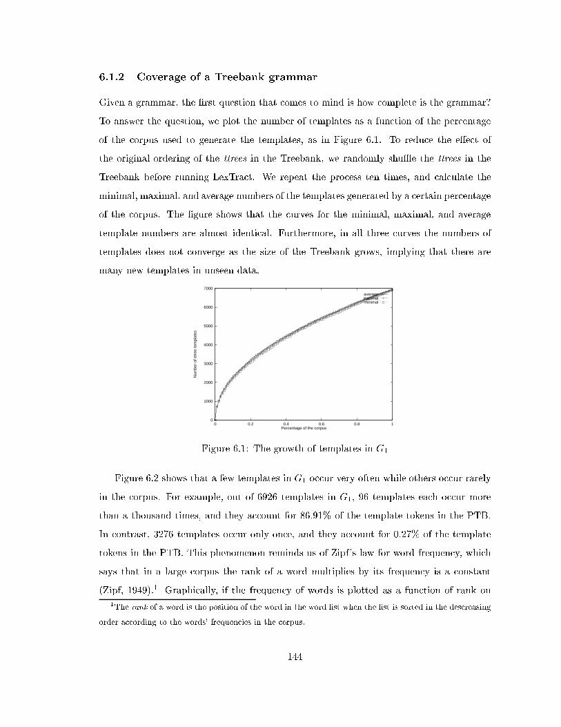
6.1.2 Coverage of a Treebank grammar
Given a grammar, the �rst question that comes to mind is how complete is the grammar?
To answer the question, we plot the number of templates as a function of the percentage
of the corpus used to generate the templates, as in Figure 6.1. To reduce the e�ect of
the original ordering of the ttrees in the Treebank, we randomly shu�e the ttrees in the
Treebank before running LexTract. We repeat the process ten times, and calculate the
minimal, maximal, and average numbers of the templates generated by a certain percentage
of the corpus. The �gure shows that the curves for the minimal, maximal, and average
template numbers are almost identical. Furthermore, in all three curves the numbers of
templates does not converge as the size of the Treebank grows, implying that there are
many new templates in unseen data.
0
1000
2000
3000
4000
5000
6000
7000
0 0.2 0.4 0.6 0.8 1
Num
ber
of e
tree
tem
plat
es
Percentage of the corpus
averagemaximalminimal
Figure 6.1: The growth of templates in G1
Figure 6.2 shows that a few templates in G1 occur very often while others occur rarely
in the corpus. For example, out of 6926 templates in G1, 96 templates each occur more
than a thousand times, and they account for 86.91% of the template tokens in the PTB.
In contrast, 3276 templates occur only once, and they account for 0.27% of the template
tokens in the PTB. This phenomenon reminds us of Zipf's law for word frequency, which
says that in a large corpus the rank of a word multiplies by its frequency is a constant
(Zipf, 1949).1 Graphically, if the frequency of words is plotted as a function of rank on
1The rank of a word is the position of the word in the word list when the list is sorted in the descreasing
order according to the words' frequencies in the corpus.
144
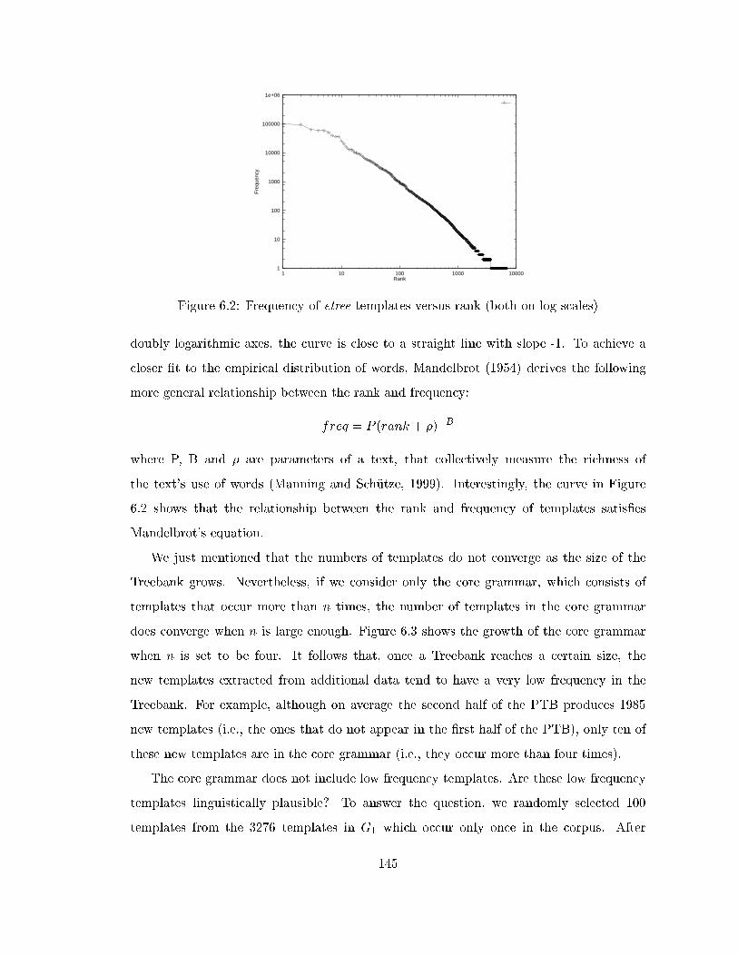
1
10
100
1000
10000
100000
1e+06
1 10 100 1000 10000
Fre
quen
cy
Rank
Figure 6.2: Frequency of etree templates versus rank (both on log scales)
doubly logarithmic axes, the curve is close to a straight line with slope -1. To achieve a
closer �t to the empirical distribution of words, Mandelbrot (1954) derives the following
more general relationship between the rank and frequency:
freq = P (rank + �)�B
where P, B and � are parameters of a text, that collectively measure the richness of
the text's use of words (Manning and Sch�utze, 1999). Interestingly, the curve in Figure
6.2 shows that the relationship between the rank and frequency of templates satis�es
Mandelbrot's equation.
We just mentioned that the numbers of templates do not converge as the size of the
Treebank grows. Nevertheless, if we consider only the core grammar, which consists of
templates that occur more than n times, the number of templates in the core grammar
does converge when n is large enough. Figure 6.3 shows the growth of the core grammar
when n is set to be four. It follows that, once a Treebank reaches a certain size, the
new templates extracted from additional data tend to have a very low frequency in the
Treebank. For example, although on average the second half of the PTB produces 1985
new templates (i.e., the ones that do not appear in the �rst half of the PTB), only ten of
these new templates are in the core grammar (i.e., they occur more than four times).
The core grammar does not include low frequency templates. Are these low frequency
templates linguistically plausible? To answer the question, we randomly selected 100
templates from the 3276 templates in G1 which occur only once in the corpus. After
145

0
200
400
600
800
1000
1200
1400
1600
1800
2000
0 0.2 0.4 0.6 0.8 1
Num
ber
of e
tree
tem
plat
es
Percentage of the corpus
averagemaximalminimal
Figure 6.3: The growth of templates in the core of G1
manually examining them, we found that 41 templates resulted from annotation errors,
two from missing entries in the language-speci�c tables that we made for the PTB, and the
remaining 57 were linguistically plausible. This experiment shows that, although the PTB
is pretty large, it is unlikely that G1 includes all the plausible templates for English.2 On
the other hand, 5276 ttrees (about 10.7% of the corpus) can produce all the 6926 templates
in G1 and 1428 ttrees (about 2.9% of the corpus) can produce all the 1967 templates in
the core grammar with the threshold set to four.3 Therefore, the question is: if we are
going to build a Treebank of a certain size from scratch, how can we choose the raw data
to maximize the number of plausible templates in the resulting Treebank grammar? If we
randomly select 5276 ttrees from the PTB, the resulting Treebank grammar has only 2360
templates (about one third the size of G1). Similarly, randomly selected 1428 ttrees yield
1263 templates, 1043 of which are in the core grammar (about half the size of the core
2Chiang (2000) did similar experiments for the tree insertion grammar that he extracted from the PTB.
His grammar has 3626 templates, of which 1587 occur once. He found that out of 100 randomly selected
once-seen templates, 34 results from annotation errors, 50 from de�ciences in the heuristics used by his
extraction algorithm, four from performance errors, and only twelve appeared to be genuine. It is hard to
compare the results of these two experiments because the Treebank grammars and the extraction algorithms
in the experiments are di�erent, as mentioned in Section 5.9.23Finding the minimal number of ttrees that generate all the templates in a grammar is a set-covering
problem, which is NP-complete. Instead of computing the minimal number, we just count the ttrees that
produce the �rst occurrence of those templates as the extraction process goes, and the counts for G1 and
the core grammar are 5276 and 1428, respectively.
146
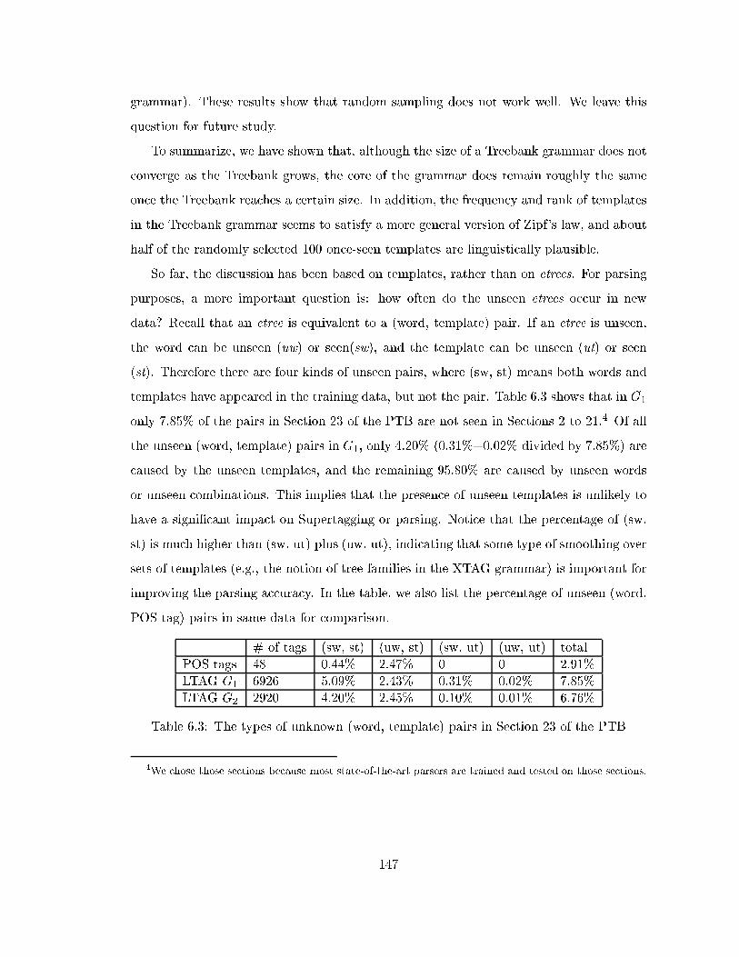
grammar). These results show that random sampling does not work well. We leave this
question for future study.
To summarize, we have shown that, although the size of a Treebank grammar does not
converge as the Treebank grows, the core of the grammar does remain roughly the same
once the Treebank reaches a certain size. In addition, the frequency and rank of templates
in the Treebank grammar seems to satisfy a more general version of Zipf's law, and about
half of the randomly selected 100 once-seen templates are linguistically plausible.
So far, the discussion has been based on templates, rather than on etrees. For parsing
purposes, a more important question is: how often do the unseen etrees occur in new
data? Recall that an etree is equivalent to a (word, template) pair. If an etree is unseen,
the word can be unseen (uw) or seen(sw), and the template can be unseen (ut) or seen
(st). Therefore there are four kinds of unseen pairs, where (sw, st) means both words and
templates have appeared in the training data, but not the pair. Table 6.3 shows that in G1
only 7.85% of the pairs in Section 23 of the PTB are not seen in Sections 2 to 21.4 Of all
the unseen (word, template) pairs in G1, only 4.20% (0.31%+0.02% divided by 7.85%) are
caused by the unseen templates, and the remaining 95.80% are caused by unseen words
or unseen combinations. This implies that the presence of unseen templates is unlikely to
have a signi�cant impact on Supertagging or parsing. Notice that the percentage of (sw,
st) is much higher than (sw, ut) plus (uw, ut), indicating that some type of smoothing over
sets of templates (e.g., the notion of tree families in the XTAG grammar) is important for
improving the parsing accuracy. In the table, we also list the percentage of unseen (word,
POS tag) pairs in same data for comparison.
# of tags (sw, st) (uw, st) (sw, ut) (uw, ut) total
POS tags 48 0.44% 2.47% 0 0 2.91%
LTAG G1 6926 5.09% 2.43% 0.31% 0.02% 7.85%
LTAG G2 2920 4.20% 2.45% 0.10% 0.01% 6.76%
Table 6.3: The types of unknown (word, template) pairs in Section 23 of the PTB
4We chose those sections because most state-of-the-art parsers are trained and tested on those sections.
147
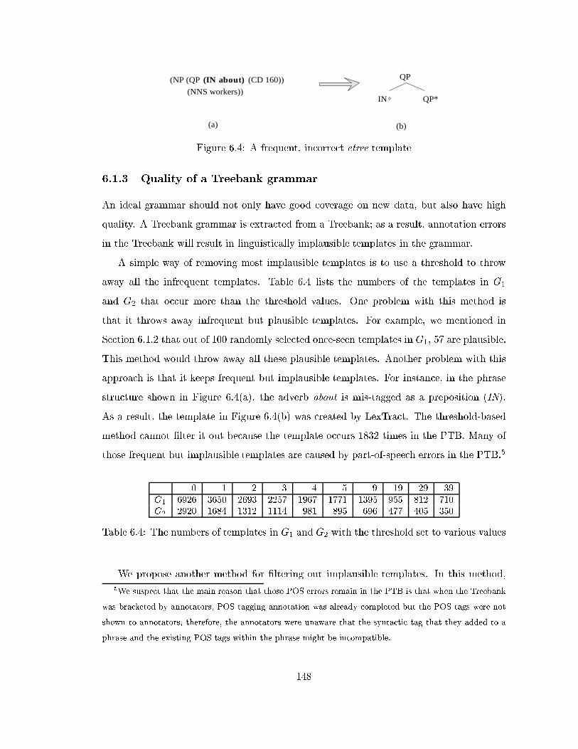
(NP (QP
(NNS workers))
QP
IN QP*
(a) (b)
(IN about) (CD 160))
Figure 6.4: A frequent, incorrect etree template
6.1.3 Quality of a Treebank grammar
An ideal grammar should not only have good coverage on new data, but also have high
quality. A Treebank grammar is extracted from a Treebank; as a result, annotation errors
in the Treebank will result in linguistically implausible templates in the grammar.
A simple way of removing most implausible templates is to use a threshold to throw
away all the infrequent templates. Table 6.4 lists the numbers of the templates in G1
and G2 that occur more than the threshold values. One problem with this method is
that it throws away infrequent but plausible templates. For example, we mentioned in
Section 6.1.2 that out of 100 randomly selected once-seen templates in G1, 57 are plausible.
This method would throw away all these plausible templates. Another problem with this
approach is that it keeps frequent but implausible templates. For instance, in the phrase
structure shown in Figure 6.4(a), the adverb about is mis-tagged as a preposition (IN).
As a result, the template in Figure 6.4(b) was created by LexTract. The threshold-based
method cannot �lter it out because the template occurs 1832 times in the PTB. Many of
those frequent but implausible templates are caused by part-of-speech errors in the PTB.5
0 1 2 3 4 5 9 19 29 39G1 6926 3650 2693 2257 1967 1771 1395 955 812 710G2 2920 1684 1312 1114 981 895 696 477 405 350
Table 6.4: The numbers of templates in G1 and G2 with the threshold set to various values
We propose another method for �ltering out implausible templates. In this method,
5We suspect that the main reason that those POS errors remain in the PTB is that when the Treebank
was bracketed by annotators, POS tagging annotation was already completed but the POS tags were not
shown to annotators; therefore, the annotators were unaware that the syntactic tag that they added to a
phrase and the existing POS tags within the phrase might be incompatible.
148

we �rst decompose a template into a set of sub-templates (see Section 5.7), then mark
the template as plausible if and only if every sub-template is plausible. The plausibility of
the subcategorization chain, the subcategorization frame, and the modi�er-modi�ee pair
are checked against the entries in the head percolation table, the argument table, and the
modi�cation table, respectively.
This �lter works well when these three tables (the head percolation table, the argument
table and the modi�cation table) are correct and complete (i.e., there are no missing entries
in the tables). In that case, the templates that are marked as implausible by the �lter are
de�nitely implausible, but not vice versa. That is, it is possible, even though unlikely,
that a template made up of plausible sub-templates is not plausible. Our �lter marks
the template in Figure 6.4(b) as implausible because a preposition (IN) cannot modify a
quanti�er phrase (QP) according to the modi�cation table.
So far, we have discussed two �lters: one is based on the frequency of the templates,
and the other checks the sub-structures of the templates. Each �lter has its strengths and
weaknesses. The choice of them should be based on the size of the Treebank, the common
types of annotation errors in the Treebank, and other factors.
6.2 Treebank grammars combined with other grammars
If a language already has a wide-coverage hand-crafted grammar such as the XTAG gram-
mar, is a Treebank grammar still useful? De�nitely. A Treebank grammar can help a
hand-crafted grammar in two ways:
� To evaluate and improve the coverage of a hand-crafted grammar on a large Treebank
� To provide statistical information to the hand-crafted grammar
In this section, we shall concentrate on the former and leave the latter for future work.
Previous evaluations (Doran et al., 2000; Srinivas et al., 1998) of hand-crafted gram-
mars use raw data (i.e., a set of sentences without syntactic bracketing). The data are �rst
parsed by an LTAG parser and the coverage of the grammar is measured as the percentage
149

of sentences in the data that can be parsed.6 For more discussion on this approach, see
(Prasad and Sarkar, 2000).
We propose a new evaluation method that takes advantage of Treebanks and LexTract.
In this method, the coverage of a hand-crafted grammar is measured by the overlap of the
hand-crafted grammar and the Treebank grammar.
6.2.1 Methodology
The central idea of our method is as follows: given a Treebank T and a grammar Gh and
letting Gt be the set of templates extracted from T by LexTract, the coverage of Gh on
T can be measured as the percentage of template tokens in T that are covered by the
intersection of Gt and Gh. One complication is that the Treebank and Gh may choose
di�erent analyses for certain syntactic constructions; that is, although some constructions
are covered by both grammars, the corresponding templates in these grammars would look
very di�erent. To account for this, our method has four stages:
1. Extract a Treebank grammar from T . Let Gt be the set of templates in the Treebank
grammar.
2. Put into G0t all the templates in Gt that match some templates in Gh.
3. Check each template in Gt � G0t and decide whether the construction represented
by the template is handled di�erently in Gh. If so, put the template in G00t . The
coverage of Gh on T is measured as count(G0t [ G00
t )=count(Gt). The templates in
Gt �G0t �G00
t are the ones that are truly missing from Gh.
4. To improve the coverage of Gh, check templates in Gt�G0t�G00
t and consider adding
the plausible ones to Gh.
In this experiment, we are focusing on general syntactic structures in two grammars,
rather than the completeness of lexicons. Therefore, for grammar coverage we use tem-
plates, instead of etrees. The method can be easily extended to compare etrees. Each stage6There should be two measures for the coverage. The �rst one is the percentage of sentences for which
the correct parses are generated; the second one is the percentage of sentences for which at least one parse
is generated.
150

of the method is described in detail as follows.
6.2.2 Stage 1: Extracting templates from Treebanks
We choose G2 as our Treebank grammar (see Table 6.2 in Section 6.1) and the XTAG
grammar as the hand-crafted grammar. The former has 2920 templates, and the latter
has 1004 templates.
6.2.3 Stage 2: Matching templates in the two grammars
To calculate the coverage of the XTAG grammar, we need to �nd out how many templates
in G2 match some template in the XTAG grammar. We de�ne two types of matching:
t-match and s-match.
t-match
An obvious distinction between the two grammars is that feature structures and subscripts7
are present only in the XTAG grammar, whereas frequency information is available only
in G2. We say that two templates t-match (t for template) if they are identical barring the
types of information present only in one grammar. In Figure 6.5, the XTAG trees in (a)
and (b) t-match the G2 tree in (c).
S
NP VP
V
S
NP VP
V
S
NP VP
V
0 1
break sleep/break
(a) pure intransitive verbs (b) ergative verbs (c) intransitive verbsin XTAG in XTAG
sleep
in G2
Figure 6.5: The templates for pure intransitive verbs and ergative verbs in XTAG t-matchthe template for all intransitive verbs in G2
7In the XTAG grammar, the subscripts on the nodes mark the same semantic arguments in related
subcategorization frames. For example, an ergative verb break can be either transitive (e.g., Mike broke the
window.) or intransitive (e.g., The window broke.). The object of the transitive frame and the subject of
the intransitive frame are both labeled as NP1, whereas the subject of the transitive frame is labeled NP0.
151

XTAG also di�ers from G2 in that XTAG uses multi-anchor trees to handle idioms
(Figure 6.6(a)), light verbs (Figure 6.6(b)) and so on.8 In each of these cases, the multiple
anchors form the predicate. By having multiple anchors, each tree can be associated
with semantic representations directly (as shown in Figure 6.6), which is an advantage
of the LTAG formalism. These trees are the spine-etrees where some arguments of the
main anchor are expanded. G2 does not have multi-anchor trees because semantics is not
marked in the Treebank and consequently LexTract cannot distinguish idiomatic meanings
from literal meanings. Since expanded subtrees are present only in the XTAG grammar,
we disregard them when comparing templates.
sem: die(NP ) 0 0 1
1
0
1
0
1
0
sem: kick(NP , NP )sem: walk(NP )0
the bucket
S
NP
kick/take
VP
V
NP VP
NP
Ntake
walk
kick
S
N
V
(a) idioms (c) transitive verbsin XTAG in XTAG
(b) light verbs in G
D
NPV
VPNP
S
NP
2
Figure 6.6: Templates in XTAG with expanded subtrees t-match the one in G2 when theexpanded subtrees are disregarded
s-match
t-match requires two trees to have exactly the same structure barring expanded subtrees;
therefore, it does not tolerate minor annotation di�erences between the two grammars.
For instance, in XTAG, a relative pronoun such as which and the complementizer that
occupy distinct positions in the template for relative clauses, whereas the Penn Treebank
treats both as pronouns and therefore they occupy the same position in G2, as shown in
Figure 6.7. Because the circled substructures occur in every template for relative clauses
and wh-movement, none of these templates would t-match their counterparts in the other
grammar. Nevertheless, the two trees share the set of sub-templates; namely, the same
subcategorization chain S ! V P ! V , the same subcategorization frame (NP, V, NP),
8For details on multi-anchor trees, see Section 2.1.4.
152

and the same modi�cation pair (NP;S). To capture this kind of similarity, we de�ne
the notion of s-match (s for sub-template). Two templates are said to s-match if they
are decomposed into the same set of sub-templates. According to this de�nition, the two
templates in Figure 6.7 s-match.
NP
NP
S NP
NP
* *
1
1
NP S
NP VP
S
NP*T*
S
NP VP
S
NP*T* V@
V@
(a) in XTAG
extroot
bar
lexroot
ext
Comp
NPnew
extroot
ext
newlexroot
(b) in G2
Figure 6.7: An example of s-match
Matching results
So far, we have de�ned two types of matching. Notice that neither type of matching is
one-to-one. Table 6.5 lists the numbers of matched templates in two grammars. The
last row lists the percentage of the template tokens in the PTB that are covered by the
templates in G2 that match some templates in XTAG. For instance, the second column
says 162 templates in XTAG t-match 54 templates in G2, and these 54 templates account
for 54.6% of the template tokens in the PTB.
t-match s-match matched unmatched totalsubtotal subtotal
XTAG 162 314 476 528 1004
G2 54 133 187 2733 2920
coverage 54.6% 5.3% 59.9% 40.1% 100%
Table 6.5: Matched templates and their coverage
Another di�erence between the XTAG and the Treebank annotation is that an adjective
modi�es a noun directly in the former, whereas in the latter an adjective projects to an
adjective phrase (AP) which in turn modi�es an NP, as shown in Figure 6.8. Similarly, in
XTAG an adverb modi�es a VP directly, whereas in the Treebank an adverb sometimes
projects to an ADVP �rst. If we disregard these annotation di�erences, the percentage
153
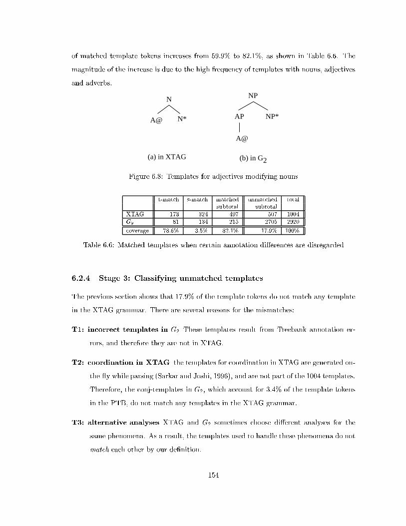
of matched template tokens increases from 59.9% to 82.1%, as shown in Table 6.6. The
magnitude of the increase is due to the high frequency of templates with nouns, adjectives
and adverbs.
N*
N
A@
NP
NP*
(a) in XTAG
AP
A@
(b) in G2
Figure 6.8: Templates for adjectives modifying nouns
t-match s-match matched unmatched totalsubtotal subtotal
XTAG 173 324 497 507 1004
G2 81 134 215 2705 2920
coverage 78.6% 3.5% 82.1% 17.9% 100%
Table 6.6: Matched templates when certain annotation di�erences are disregarded
6.2.4 Stage 3: Classifying unmatched templates
The previous section shows that 17.9% of the template tokens do not match any template
in the XTAG grammar. There are several reasons for the mismatches:
T1: incorrect templates in G2 These templates result from Treebank annotation er-
rors, and therefore they are not in XTAG.
T2: coordination in XTAG the templates for coordination in XTAG are generated on-
the- y while parsing (Sarkar and Joshi, 1996), and are not part of the 1004 templates.
Therefore, the conj-templates in G2, which account for 3.4% of the template tokens
in the PTB, do not match any templates in the XTAG grammar.
T3: alternative analyses XTAG and G2 sometimes choose di�erent analyses for the
same phenomena. As a result, the templates used to handle these phenomena do not
match each other by our de�nition.
154

T4: constructions not covered by XTAG Some constructions, such as the unlike co-
ordination phrase (UCP), parenthetical (PRN), and ellipsis, are not currently covered
by the XTAG grammar.
For the �rst three types, the XTAG grammar can handle the corresponding construc-
tions although the templates used in two grammars look di�erent and do not match ac-
cording to our de�nition. To �nd out what constructions are not covered by XTAG, we
manually classi�ed the 289 most frequent unmatched templates in G2 according to the
reason that they are absent from XTAG. These 289 templates account for 93.9% of all the
unmatched template tokens in the Treebank. The results are shown in Table 6.7, where the
percentage is with respect to all the tokens in the Treebank. From the table, it is clear that
most unmatched template tokens are due to (T3); that is, alternative analyses adopted in
the two grammars. Combining the results in Table 6.6 and 6.7, we conclude that 97.2%
of template tokens in the Treebank are covered by XTAG,9 while another 1.7% are not
covered. The remaining 1.1% of template tokens are covered by the 2416 unmatched tem-
plates in G2, which we have not checked manually. Therefore, it is not clear how many of
this remaining 1.1% template tokens are covered by XTAG.
T1 T2 T3 T4 total
# of template types 51 52 93 93 289
% of template tokens 1.1% 3.4% 10.6% 1.7% 16.8%
Table 6.7: Classi�cation of 289 unmatched templates
6.2.5 Stage 4: Combining two grammars
Given the XTAG grammar and the Treebank grammar, simply taking the union of two
template sets will yield an inconsistent grammar. One way of improving the coverage of
the XTAG grammar is to analyze the constructions in T4, build new trees for them (or
use the corresponding trees in the Treebank grammar), and add these trees to the XTAG
grammar.
9The number 97.2% is the sum of two numbers: the �rst one is the percentage of matched template
tokens (82.1% from Table 6.6). The second number is the percentage of template tokens in T1|T3 (16.8%-
1.7%=15.1% from Table 6.7).
155
Another possibility is to use LexOrg to generate a new grammar. This process has
several steps. First, LexTract decomposes templates in both grammars into a set of sub-
templates such as subcategorization chains, subcategorization frames, and modi�cation
pairs. Second, we use LexTract's �lter to automatically rule out all the implausible sub-
templates in XTAG and G2. Third, we manually check the remaining sub-templates. If
two grammars adopt di�erent treatments for a certain construction, choose one treatment
and its corresponding sub-templates. Last, we use LexOrg to generate a new grammar
from these sub-templates. The new grammar will be consistent and have a good coverage
of the Treebank. We plan to explore this possibility in the future.
To summarize this section, we have presented a method for evaluating the coverage of a
hand-crafted grammar | the XTAG grammar | on a Treebank. First, we used LexTract
to automatically extract a Treebank grammar. Second, we matched the templates in
the two grammars. Third, we manually classi�ed unmatched templates in the Treebank
grammar to decide how many of them were due to missing constructions in the hand-crafted
grammar. Some of the unmatched templates can be added to the hand-crafted grammar
to improve its coverage. Our experiments showed that the XTAG grammar could cover at
least 97.2% of the template tokens in the English Penn Treebank.
This method has several advantages. First, the whole process is semi-automatic and
requires little human e�ort. Second, the coverage can be calculated at the sentence level,
template level and sub-structure level. Third, the method provides a list of templates that
can be added to the grammar to improve its coverage. Fourth, there is no need to parse
the whole corpus, which could have been very time-consuming.
6.3 Comparison of Treebank grammars for di�erent lan-
guages
In the last section, we compared a hand-crafted grammar with a Treebank grammar. In
this section, we shall compare grammars for di�erent languages for two reasons. First, we
want to know how similar or di�erent the languages are with respect to the elementary
trees in their grammars. Second, the links between the elementary trees in the grammars
156
are valuable resources for NLP applications such as machine translation (MT).
To compare grammars for di�erent languages, we can choose either hand-crafted gram-
mars or Treebank grammars. We chose Treebank grammars for the following reasons.
First, Treebank grammars can be easily extracted from Treebanks with little human ef-
fort. Second, the extracted grammars are guaranteed to cover the source Treebanks. Third,
the grammars built by the same extraction tool are based on the same formalisms, making
grammar comparison possible. A potential problem for using Treebank grammars is that
the grammars may include linguistic implausible templates while missing plausible ones
due to the imperfection of the source Treebanks. To alleviate this problem, a threshold-
based �lter is used to throw away low frequency templates.
Our approach for grammar comparison has three stages: First, we extract grammars
from Treebanks; Second, given a grammar pair, we count the number of templates that
appear in both grammars; Third, we classify the templates that appear in one but not
in the other grammar. In this section, we �rst introduce the three Treebanks used for
grammar comparison. Then, we report experimental results on grammar comparison.
Next, we point out the directions for future work.
6.3.1 Three Treebanks for three languages
The languages whose grammars are being compared are English, Chinese, and Korean.
They belong to di�erent language families: English is Germanic, Chinese is Sino-Tibetan,
and Korean is Altaic (Comrie, 1987). There are several major di�erences between these
languages. First, both English and Chinese have predominantly subject-verb-object (SVO)
word order, whereas Korean has underlying SOV order. Second, the word order in Korean
is freer than in English and Chinese in the sense that argument NPs are freely permutable
(subject to certain discourse constraints). Third, Korean and Chinese allow subject and
object deletion, but English does not. Fourth, Korean has richer in ectional morphology
than English, whereas Chinese has little, if any, in ectional morphology.
The Treebanks that we used in this section are the English Penn Treebank II (Marcus et
al., 1993), the Chinese Penn Treebank (Xia et al., 2000b), and the Korean Penn Treebank
(Han et al., 2001). All three Treebanks were developed at the University of Pennsylvania
157

in the last decade. The main parameters of these Treebanks are summarized in Table 6.8.
The tagsets include four types of tags: POS tags for head-level annotation, syntactic tags
for phrase-level annotation, function tags for grammatical function annotation, and empty
category (EC) tags for dropped arguments, traces, and so on. The average sentence length
for the Korean Treebank is much shorter than those for English and Chinese because the
Korean Treebank is a collection of military messages, whereas English and Chinese corpora
consist of newspaper articles. Because the Korean Treebank is a small corpus of a limited
sub-language, we shall mainly focus on the comparison between the English and Chinese
grammars.
Language corpus size ave sentence POS syntactic function EC(words) length (words) tags tags tags tags
English 1,174K 23.85 words 36 26 20 10Chinese 100K 23.81 words 34 25 26 7Korean 54K 10.71 words 27 14 6 4
Table 6.8: Sizes of the Treebanks and their tagsets
We chose these Treebanks for two reasons: First, their annotation schemata are similar,
which facilitates the comparison between the extracted Treebank grammars. For example,
all three Treebanks use phrase structures, rather than dependency structures. They all
include empty categories, reference indexes, and function tags in addition to syntactic
labels. Second, all three Treebanks were designed by linguists and computational linguists
and the annotation were at least double checked. Therefore, the grammars extracted from
the Treebanks should have good quality.
The results of running LexTract on English, Chinese, and Korean Treebanks are shown
in Table 6.9. The last column in the table shows the numbers of the non-lexicalized context-
free rules.
template etree word context-freetypes types types rules
English 6926 131,397 49,206 1524
Chinese 1140 21,125 10,772 515
Korean 632 13,941 10,035 152
Table 6.9: Grammars extracted from the three Treebanks
158
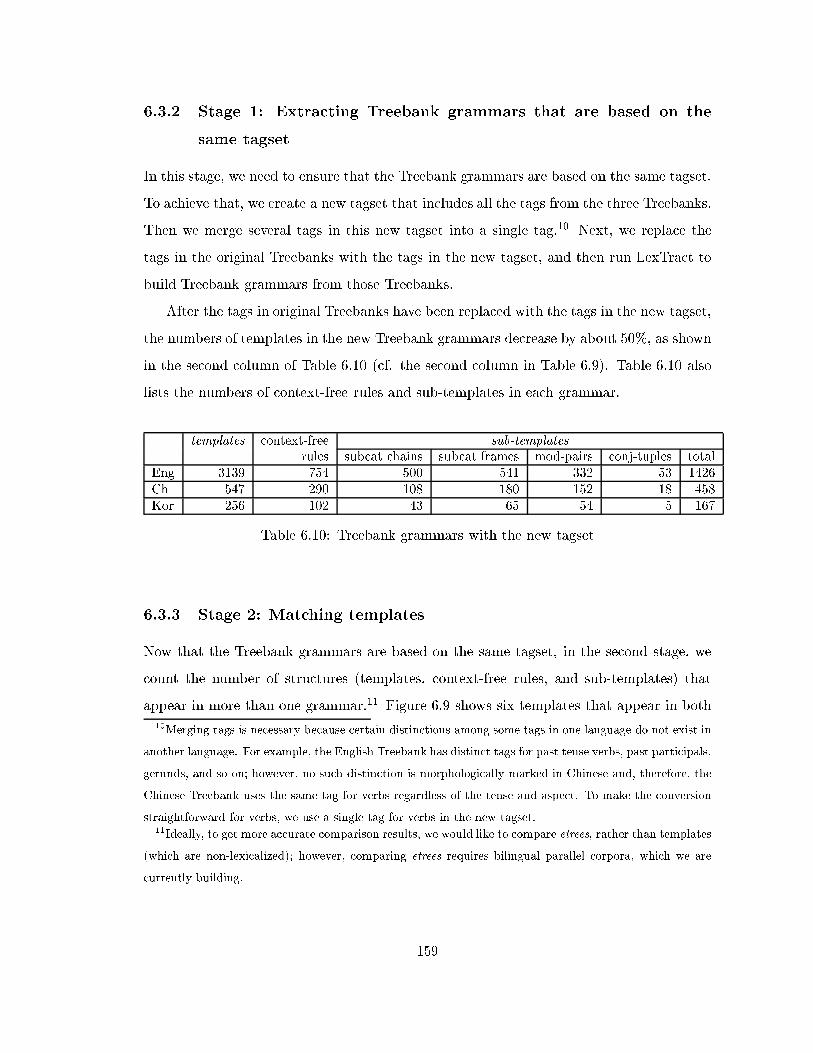
6.3.2 Stage 1: Extracting Treebank grammars that are based on the
same tagset
In this stage, we need to ensure that the Treebank grammars are based on the same tagset.
To achieve that, we create a new tagset that includes all the tags from the three Treebanks.
Then we merge several tags in this new tagset into a single tag.10 Next, we replace the
tags in the original Treebanks with the tags in the new tagset, and then run LexTract to
build Treebank grammars from those Treebanks.
After the tags in original Treebanks have been replaced with the tags in the new tagset,
the numbers of templates in the new Treebank grammars decrease by about 50%, as shown
in the second column of Table 6.10 (cf. the second column in Table 6.9). Table 6.10 also
lists the numbers of context-free rules and sub-templates in each grammar.
templates context-free sub-templates
rules subcat chains subcat frames mod-pairs conj-tuples totalEng 3139 754 500 541 332 53 1426Ch 547 290 108 180 152 18 458Kor 256 102 43 65 54 5 167
Table 6.10: Treebank grammars with the new tagset
6.3.3 Stage 2: Matching templates
Now that the Treebank grammars are based on the same tagset, in the second stage, we
count the number of structures (templates, context-free rules, and sub-templates) that
appear in more than one grammar.11 Figure 6.9 shows six templates that appear in both
10Merging tags is necessary because certain distinctions among some tags in one language do not exist in
another language. For example, the English Treebank has distinct tags for past tense verbs, past participals,
gerunds, and so on; however, no such distinction is morphologically marked in Chinese and, therefore, the
Chinese Treebank uses the same tag for verbs regardless of the tense and aspect. To make the conversion
straightforward for verbs, we use a single tag for verbs in the new tagset.11Ideally, to get more accurate comparison results, we would like to compare etrees, rather than templates
(which are non-lexicalized); however, comparing etrees requires bilingual parallel corpora, which we are
currently building.
159

NP
N@
VP
V@ VP*
NP
N@ NP*ADV@
VP
ADVP VP*
S
VPNP
V@ S
S
NP VP
V@ NP
α
β
1:
3:
β1:β2:
α 3:α 2:
9.98%/12.03% 0.90%/4.94%20.91%/20.83%
6.31%/0.81% 1.50%/2.18% 1.33%/1.08%
Figure 6.9: Some templates that appear in both the English and Chinese grammars
the English and the Chinese grammars.12 The numbers x/y under each template are
the percentages of the template tokens in the English Treebank (ETB) and the Chinese
Treebank (CTB), respectively. For example, the numbers under �1 says that the template
accounts for 20.91% of template tokens in the ETB, and 20.83% in the CTB.
Initial results
Table 6.11 lists the number of matched templates for each language pair. The third column
lists the numbers of template types shared by each pair of Treebank grammars and the
percentage of the template tokens in each Treebank that are covered by these matched
template types. For example, there are 237 template types that appear in both English
and Chinese Treebank grammars. These 237 template types account for 80.1% of the
template tokens in the ETB, and 81.5% of the template tokens in the CTB. There are
a few things worth mentioning. First, although the numbers of matched templates are
not very high, some of these templates have high frequency and therefore the percentages
of matched template tokens are pretty high. For example, the six templates in Figure
6.9 accounts for 40.95% of template tokens in the ETB and 41.90% in the CTB. Second,
the frequency of the same template in di�erent Treebanks may di�er substantially. For
example, �3 in Figure 6.9 accounts for 6.31% of template tokens in the ETB but 0.81% in
the CTB, while �2 accounts for 0.90% in the ETB but 4.94% in the CTB. A major reasons
12�1, �1, and �2 also appear in the Korean grammar. For �3, �2, and �3, if we reverse the positions of
the verb and its sister, the resulting templates are in the Korean grammar as well.
160

for this di�erence is that the set of words that anchor the same template may di�er across
languages; that is, if a word w in language l anchors a template f , it is possible that
the translation of w in language l0 does not anchor f . For example, in English the �3 is
anchored by auxiliary verbs including modals, be verbs as in progressive (e.g., is eating)
and passive (e.g., is eaten), and have verbs as in present perfect (e.g., have eaten). In
contrast, in Chinese the �3 is anchored only by modals. The be and have verbs in English
are translated into adverbs or aspect markers in Chinese. The adverbs anchor �2, and the
template for the aspect markers appears only in the Chinese grammar.
templates context-free rules sub-templates(Eng, Ch) type (#) 237 154 246
token (%) 80.1/81.5 88.0/85.2 91.4/85.2(Eng, Kor) type (#) 54 61 96
token (%) 47.6/85.6 53.4/92.2 58.9/98.4(Ch, Kor) type (#) 43 44 69
token (%) 55.9/81.0 63.2/89.3 65.7/96.0
Table 6.11: Numbers of matched templates, context-free rules, and sub-templates in threegrammar pairs
If we compare context-free rules, rather than templates, the percentages of matched
context-free rules (as shown in the fourth column in Table 6.11) are higher than the
percentages of matched template tokens. This is because two distinct templates may share
common context-free rules. Similarly, the percentages of matched sub-templates (see the
last column in Table 6.11) are higher than the percentages of matched template tokens.
Results using thresholds
The comparison results shown in Table 6.11 used every template in the Treebank gram-
mars regardless of the frequency of the template in the corresponding Treebank. One
potential problem with this approach is that annotation errors in the Treebanks could
have a substantial e�ect on the comparison results. One such scenario is as follows: To
compare languages A and B, we use Treebanks TA for language A and Treebank TB for
language B. Let GA and GB be the grammars extracted from TA and TB, respectively, and
let t be a template that appears in both grammars. Now suppose that t is a linguistically
161
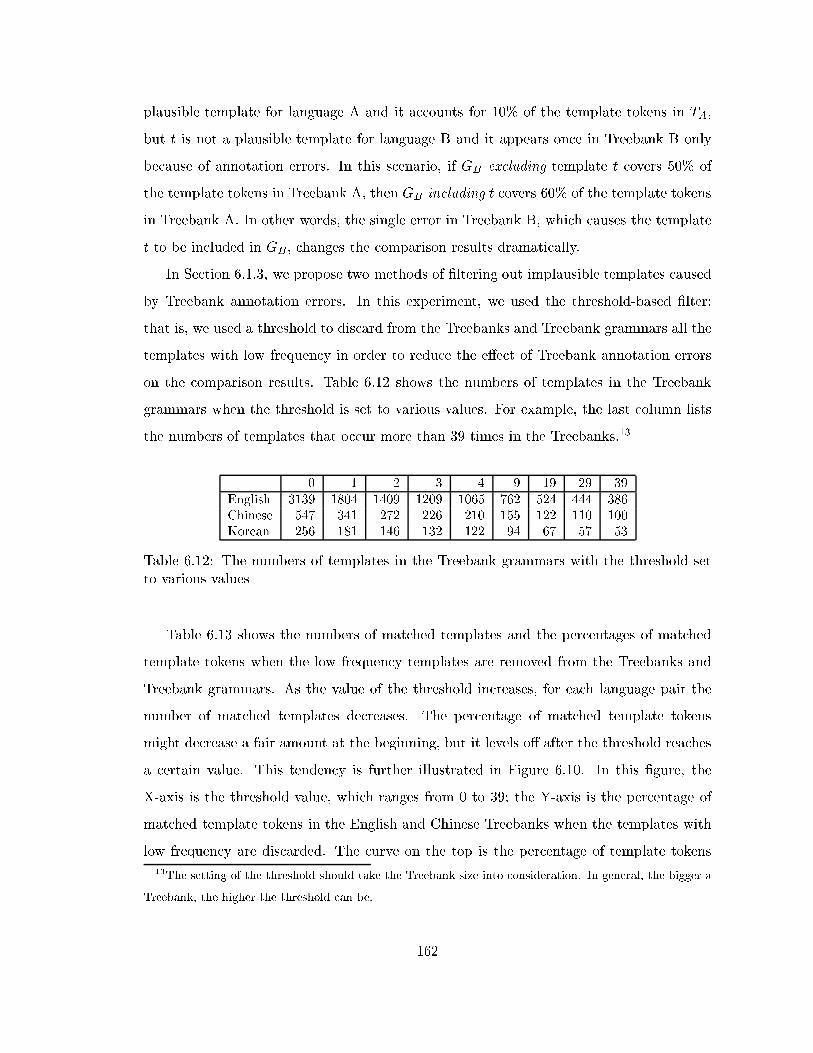
plausible template for language A and it accounts for 10% of the template tokens in TA,
but t is not a plausible template for language B and it appears once in Treebank B only
because of annotation errors. In this scenario, if GB excluding template t covers 50% of
the template tokens in Treebank A, then GB including t covers 60% of the template tokens
in Treebank A. In other words, the single error in Treebank B, which causes the template
t to be included in GB , changes the comparison results dramatically.
In Section 6.1.3, we propose two methods of �ltering out implausible templates caused
by Treebank annotation errors. In this experiment, we used the threshold-based �lter;
that is, we used a threshold to discard from the Treebanks and Treebank grammars all the
templates with low frequency in order to reduce the e�ect of Treebank annotation errors
on the comparison results. Table 6.12 shows the numbers of templates in the Treebank
grammars when the threshold is set to various values. For example, the last column lists
the numbers of templates that occur more than 39 times in the Treebanks.13
0 1 2 3 4 9 19 29 39English 3139 1804 1409 1209 1065 762 524 444 386Chinese 547 341 272 226 210 155 122 110 100Korean 256 181 146 132 122 94 67 57 53
Table 6.12: The numbers of templates in the Treebank grammars with the threshold setto various values
Table 6.13 shows the numbers of matched templates and the percentages of matched
template tokens when the low frequency templates are removed from the Treebanks and
Treebank grammars. As the value of the threshold increases, for each language pair the
number of matched templates decreases. The percentage of matched template tokens
might decrease a fair amount at the beginning, but it levels o� after the threshold reaches
a certain value. This tendency is further illustrated in Figure 6.10. In this �gure, the
X-axis is the threshold value, which ranges from 0 to 39; the Y-axis is the percentage of
matched template tokens in the English and Chinese Treebanks when the templates with
low frequency are discarded. The curve on the top is the percentage of template tokens
13The setting of the threshold should take the Treebank size into consideration. In general, the bigger a
Treebank, the higher the threshold can be.
162

0.3
0.4
0.5
0.6
0.7
0.8
0.9
0 5 10 15 20 25 30 35
Per
cent
age
of m
atch
ed te
mpl
ate
toke
ns
Cutoffs
EnglishChinese
Figure 6.10: The percentages of matched template tokens in the English and ChineseTreebanks with various threshold values
in the Chinese Treebank that are covered by the English grammar, and the curve on the
bottom is the percentage of template tokens in the English Treebank that are covered by
the Chinese grammar. Both curves become almost at once the threshold value reaches 5
or larger.
threshold 0 1 2 3 4 5 19
(Eng, type (#) 237 165 128 111 100 73 54Ch) token (%) 80.1/81.5 76.5/80.8 64.3/80.6 64.1/80.6 63.8/78.5 58.1/77.9 57.3/76.9
(Eng, type (#) 54 47 37 35 32 29 23Kor) token (%) 47.6/85.6 47.5/81.0 47.2/81.0 47.3/80.7 47.3/80.7 47.3/80.4 47.5/79.3
(Ch, type (#) 43 36 34 29 27 22 18Kor) token (%) 55.9/81.0 56.0/81.0 56.0/77.0 56.1/76.0 55.8/76.1 56.0/74.3 56.1/74.5
Table 6.13: Matched templates in the Treebank grammars with various threshold values
To summarize, in order to get a better estimate of the percentage of matched template
tokens, we disregard the low frequency templates in the Treebanks. We hope that this
strategy reduces the e�ect of annotation errors on the comparison results. This strategy
also makes the di�erence between the sizes of the three Treebanks less important because,
once a Treebank reaches a certain size, the new templates extracted from additional data
tend to have very low frequency in the whole Treebank (See Section 6.1.2) and they will
be thrown away by the threshold-based �lter.
163
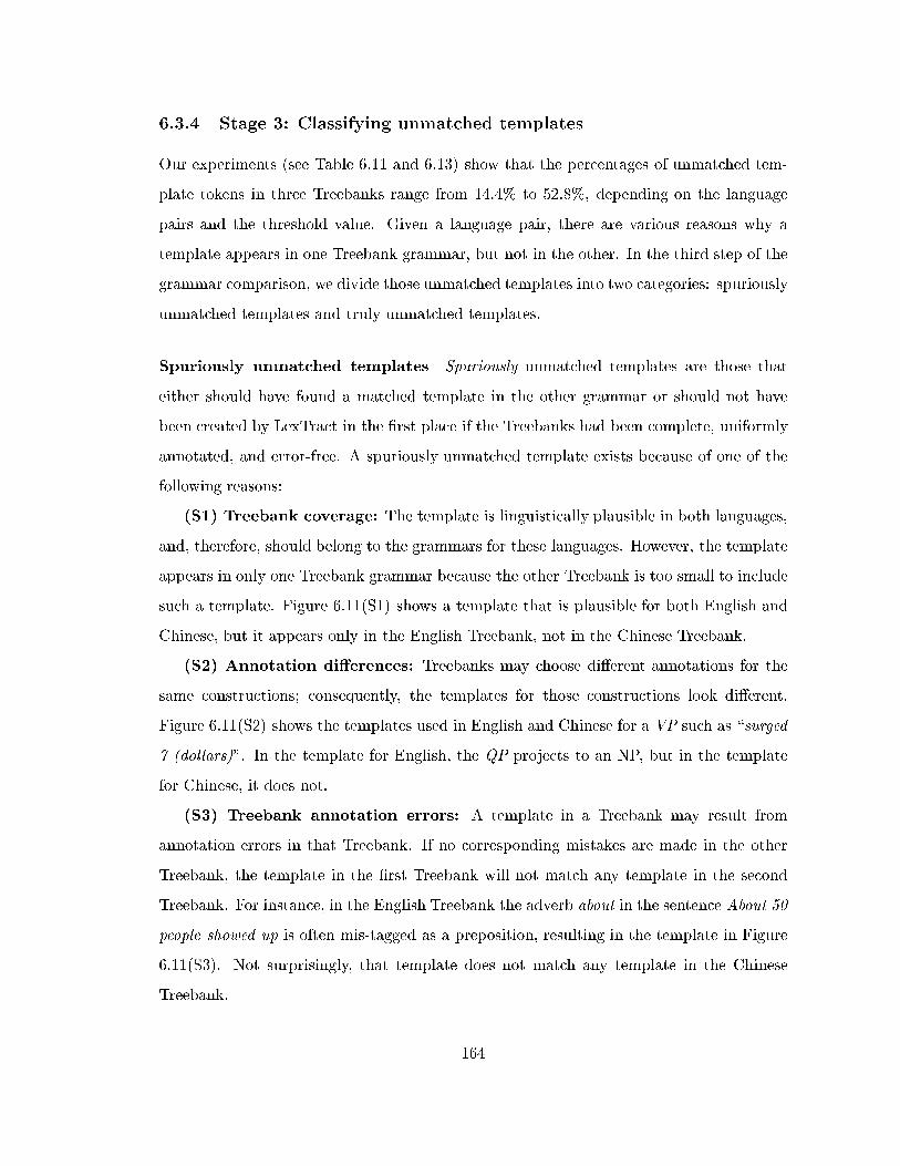
6.3.4 Stage 3: Classifying unmatched templates
Our experiments (see Table 6.11 and 6.13) show that the percentages of unmatched tem-
plate tokens in three Treebanks range from 14.4% to 52.8%, depending on the language
pairs and the threshold value. Given a language pair, there are various reasons why a
template appears in one Treebank grammar, but not in the other. In the third step of the
grammar comparison, we divide those unmatched templates into two categories: spuriously
unmatched templates and truly unmatched templates.
Spuriously unmatched templates Spuriously unmatched templates are those that
either should have found a matched template in the other grammar or should not have
been created by LexTract in the �rst place if the Treebanks had been complete, uniformly
annotated, and error-free. A spuriously unmatched template exists because of one of the
following reasons:
(S1) Treebank coverage: The template is linguistically plausible in both languages,
and, therefore, should belong to the grammars for these languages. However, the template
appears in only one Treebank grammar because the other Treebank is too small to include
such a template. Figure 6.11(S1) shows a template that is plausible for both English and
Chinese, but it appears only in the English Treebank, not in the Chinese Treebank.
(S2) Annotation di�erences: Treebanks may choose di�erent annotations for the
same constructions; consequently, the templates for those constructions look di�erent.
Figure 6.11(S2) shows the templates used in English and Chinese for a VP such as \surged
7 (dollars)". In the template for English, the QP projects to an NP, but in the template
for Chinese, it does not.
(S3) Treebank annotation errors: A template in a Treebank may result from
annotation errors in that Treebank. If no corresponding mistakes are made in the other
Treebank, the template in the �rst Treebank will not match any template in the second
Treebank. For instance, in the English Treebank the adverb about in the sentence About 50
people showed up is often mis-tagged as a preposition, resulting in the template in Figure
6.11(S3). Not surprisingly, that template does not match any template in the Chinese
Treebank.
164
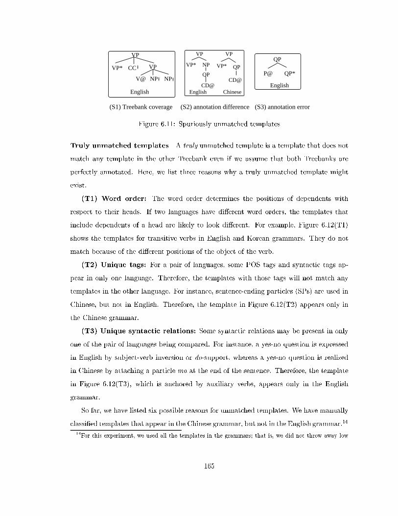
VP*
VP
CC
V@ NP NP
VP
English English ChineseCD@
QP
NPVP*
VP VP
VP* QP
CD@
QP
P@ QP*
English
(S1) Treebank coverage (S2) annotation difference (S3) annotation error
Figure 6.11: Spuriously unmatched templates
Truly unmatched templates A truly unmatched template is a template that does not
match any template in the other Treebank even if we assume that both Treebanks are
perfectly annotated. Here, we list three reasons why a truly unmatched template might
exist.
(T1) Word order: The word order determines the positions of dependents with
respect to their heads. If two languages have di�erent word orders, the templates that
include dependents of a head are likely to look di�erent. For example, Figure 6.12(T1)
shows the templates for transitive verbs in English and Korean grammars. They do not
match because of the di�erent positions of the object of the verb.
(T2) Unique tags: For a pair of languages, some POS tags and syntactic tags ap-
pear in only one language. Therefore, the templates with those tags will not match any
templates in the other language. For instance, sentence-ending particles (SPs) are used in
Chinese, but not in English. Therefore, the template in Figure 6.12(T2) appears only in
the Chinese grammar.
(T3) Unique syntactic relations: Some syntactic relations may be present in only
one of the pair of languages being compared. For instance, a yes-no question is expressed
in English by subject-verb inversion or do-support, whereas a yes-no question is realized
in Chinese by attaching a particle ma at the end of the sentence. Therefore, the template
in Figure 6.12(T3), which is anchored by auxiliary verbs, appears only in the English
grammar.
So far, we have listed six possible reasons for unmatched templates. We have manually
classi�ed templates that appear in the Chinese grammar, but not in the English grammar.14
14For this experiment, we used all the templates in the grammars; that is, we did not throw away low
165
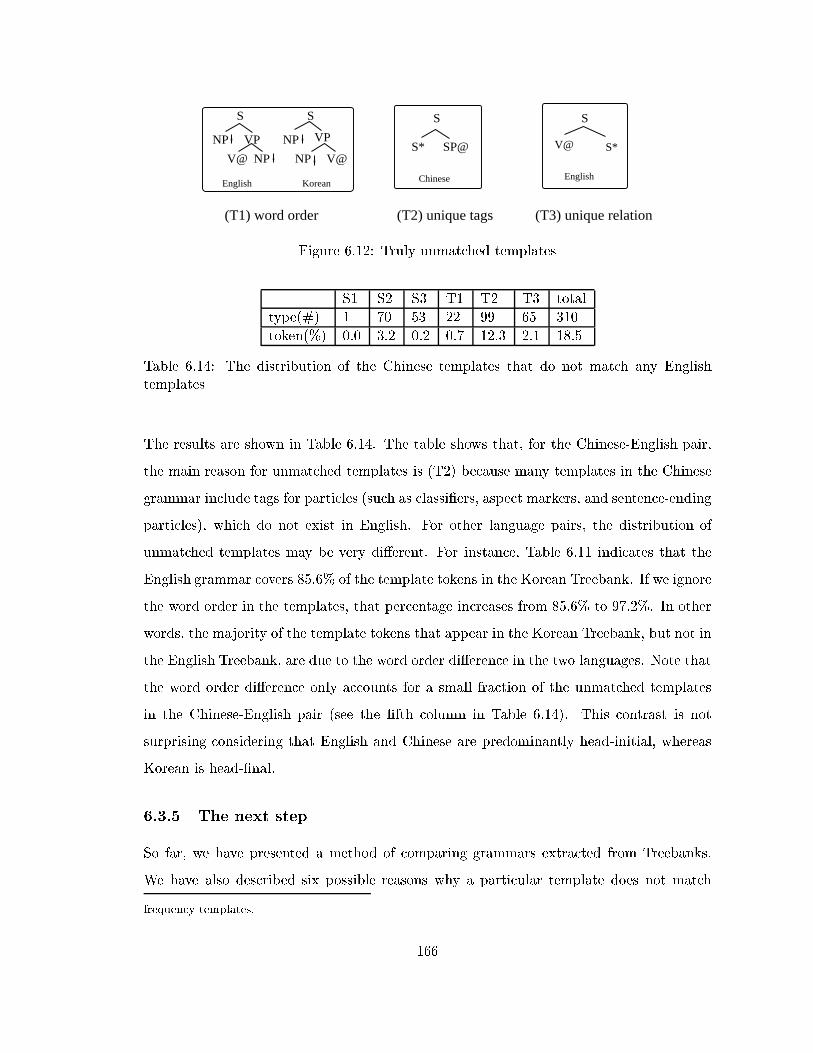
NPV@
VPNP
S
V@
NP
S
VP
NP
English Korean
(T3) unique relation(T2) unique tags(T1) word order
SP@S*
S
Chinese English
V@ S*
S
Figure 6.12: Truly unmatched templates
S1 S2 S3 T1 T2 T3 total
type(#) 1 70 53 22 99 65 310
token(%) 0.0 3.2 0.2 0.7 12.3 2.1 18.5
Table 6.14: The distribution of the Chinese templates that do not match any Englishtemplates
The results are shown in Table 6.14. The table shows that, for the Chinese-English pair,
the main reason for unmatched templates is (T2) because many templates in the Chinese
grammar include tags for particles (such as classi�ers, aspect markers, and sentence-ending
particles), which do not exist in English. For other language pairs, the distribution of
unmatched templates may be very di�erent. For instance, Table 6.11 indicates that the
English grammar covers 85.6% of the template tokens in the Korean Treebank. If we ignore
the word order in the templates, that percentage increases from 85.6% to 97.2%. In other
words, the majority of the template tokens that appear in the Korean Treebank, but not in
the English Treebank, are due to the word order di�erence in the two languages. Note that
the word order di�erence only accounts for a small fraction of the unmatched templates
in the Chinese-English pair (see the �fth column in Table 6.14). This contrast is not
surprising considering that English and Chinese are predominantly head-initial, whereas
Korean is head-�nal.
6.3.5 The next step
So far, we have presented a method of comparing grammars extracted from Treebanks.
We have also described six possible reasons why a particular template does not match
frequency templates.
166

any templates in another language. An ummatched template that include unique tags or
unique syntactic relations (i.e., (T2) and (T3)) often indicates that the two languages in
the language pair express certain syntactic features in di�erent ways. For example, a yes-
no question is realized in Chinese by attaching a particle ma at the end of the sentence;
that is, ma anchors the template in Figure 6.12(T2). In contrast, a yes-no question is
realized in English by subject-verb inversion or do-support; that is, auxiliary verbs anchor
the template in Figure 6.12(T3). A MT system should pay attention to the di�erence and
handle the templates properly.
In addition to building Treebank grammars, LexTract can also be used to build etree-
to-etree mappings automatically from parallel Treebanks. The process can be simpli�ed
as follows:
(1) Run bitext mapping algorithms, such as the Smooth Injective Map Recognizer (SIMR)
algorithm (Melamed, 1999), on parallel Treebanks to align sentences and produce a
word-to-word mapping function in the aligned sentences.
(2) For each aligned sentence pair, run LexTract to produce grammars and derivation
trees from the ttrees.
(3) Link the nodes in the derivation trees using the word-to-word mapping, thus, creating
a etree-to-etree mapping.
This process is illustrated in Figure 6.13. In (a), T and T 0 are two ttrees in a parallel
English-Chinese Treebank. In (b), a bitext mapping algorithm decides that the sentences
in T and T 0 form a parallel sentence pair. Then it builds the word-to-word mapping fw.
In (c), LexTract produces Treebank grammars G and G0 and the derivation trees D and
D0 for the sentences. In (d), the etree-to-etree mapping function ft is created.
Quite often, the translation of a word consists of several words in another language.
For instance, in Figure 6.14(a), the word q�u in Chinese is translated into go to in English
and the word did in English roughly corresponds to le ma in Chinese.15 As a result, the
15The sentence-ending particle ma in Chinese indicates that the sentence is a yes-no question, whereas
in English the same information is expressed by subject-verb inversion or do-support. The sentence-ending
particle le in Chinese indicates that the action q�u x�uexi�ao/go to school happens in the past, whereas in
167
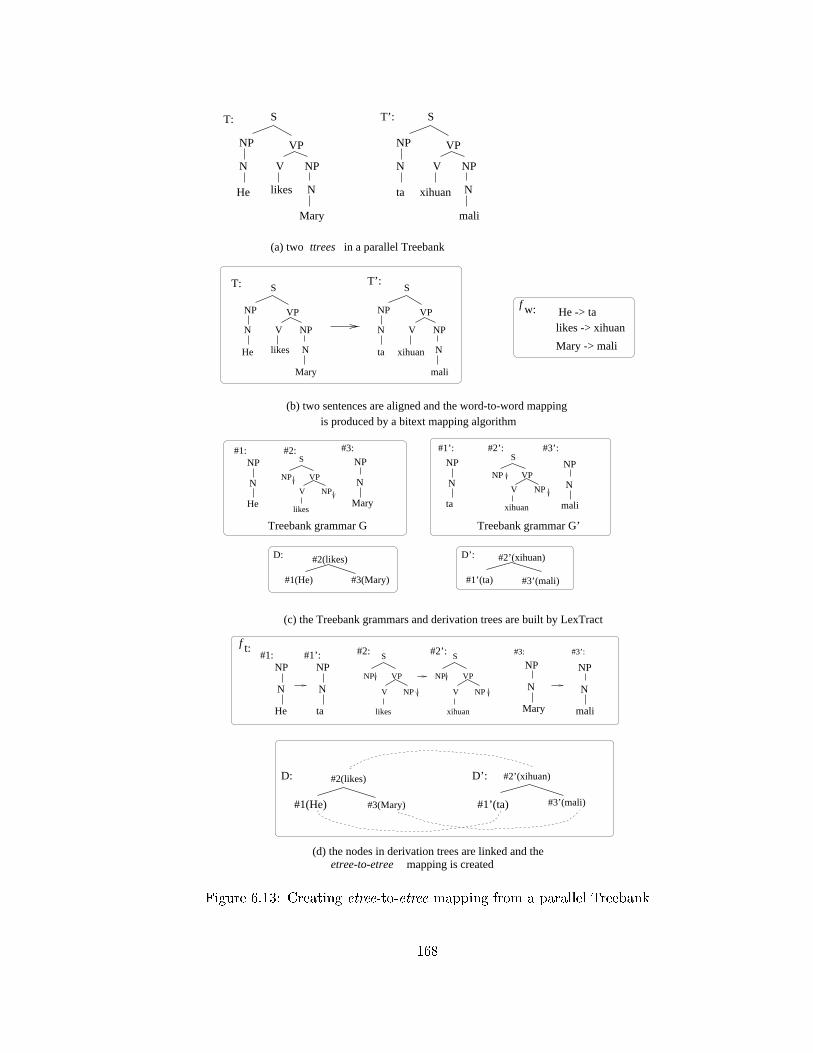
NP VP
N V NP
N
S
NP VP
N V
likes
NP
N
Mary
S
He ta xihuan
mali
T:
NP VP
N V NP
N
S
NP VP
N V
likes
NP
N
Mary
S
He ta xihuan
mali
T’:
(d) the nodes in derivation trees are linked and the etree-to-etree mapping is created
NP
N
He
NP
N
ta
#1’:#1:
NP
N
He
NP
N
ta
S
VPNP
V NP
likes
NP
Mary
N
S
VPNP
V NP
xihuan
NP
mali
N
S
VPNP
V NP
likes
S
VPNP
V NP
xihuan
NP
Mary
N
NP
mali
N
(a) two ttrees in a parallel Treebank
T: T’:
(b) two sentences are aligned and the word-to-word mapping is produced by a bitext mapping algorithm
(c) the Treebank grammars and derivation trees are built by LexTract
f t:
He -> talikes -> xihuan
Mary -> mali
f w:
#1: #2: #3:
Treebank grammar G
#1’: #2’: #3’:
Treebank grammar G’
#2(likes)
#1(He) #3(Mary)
D:
#1’(ta)
D’: #2’(xihuan)
#3’(mali)
#2: #3: #3’:#2’:
#1(He)
D:
#1’(ta)
D’:
#3(Mary)
#2’(xihuan)
#3’(mali)
#2(likes)
Figure 6.13: Creating etree-to-etree mapping from a parallel Treebank
168
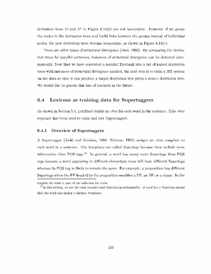
derivation trees D and D0 in Figure 6.14(b) are not isomorphic. However, if we group
the nodes in the derivation trees and build links between the groups instead of individual
nodes, the new derivation trees become isomorphic, as shown in Figure 6.14(c).
There are other types of structural divergence (Dorr, 1993). By comparing the deriva-
tion trees for parallel sentences, instances of structural divergence can be detected auto-
matically. Now that we have converted a parallel Treebank into a list of paired derivation
trees with instances of structural divergence marked, the next step is to train a MT system
on the data so that it can produce a target derivation tree given a source derivation tree.
We would like to pursue this line of research in the future.
6.4 Lexicons as training data for Supertaggers
As shown in Section 5.4, LexTract builds an etree for each word in the sentence. This etree
sequence has been used to train and test Supertaggers.
6.4.1 Overview of Supertaggers
A Supertagger (Joshi and Srinivas, 1994; Srinivas, 1997) assigns an etree template to
each word in a sentence. The templates are called Supertags because they include more
information than POS tags.16 In general, a word has many more Supertags than POS
tags because a word appearing in di�erent elementary trees will have di�erent Supertags
whereas its POS tag is likely to remain the same. For example, a preposition has di�erent
Supertags when the PP headed by the preposition modi�es a VP, an NP, or a clause. In the
English the tense is part of the in ection for verbs.16In this section, we use the term template and Supertag interchangeably. A word has x Supertags means
that the word can anchor x distinct templates.
169
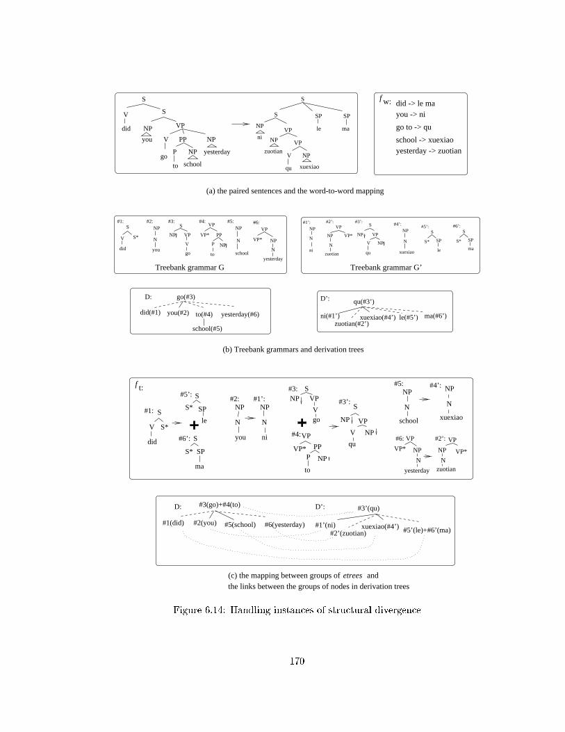
V
V
P
did
goto
NP
PP
school
yesterday
NPyou
NP
S
S
VP
S
VP
VP
V NP
SP SP
S
qu
NP
ni NP
zuotian
xuexiao
le ma
S*
S
V
did
#1:NP
N
you
#2:
PP
P
to
VP*
VP
NP
#4:
NP
S
VP
go
V
#3:NP
N
school
#5:
VP
VP* NP
N
yesterday
#6:NP
N
ni
#1’:
NP VP*
N
VP
zuotian
#2’:
NP
S
qu
NP VP
V
#3’:
NP
N
xuexiao
#4’:
S
SP
le
S*
#5’:S
SPS*
ma
#6’:
D’:
ni(#1’)zuotian(#2’)
xuexiao(#4’) ma(#6’)le(#5’)
qu(#3’)D:
did(#1)
school(#5)
to(#4)you(#2)
go(#3)
yesterday(#6)
#2’: VP
VP*NP
Nzuotian
#6:
yesterday
VP
VP* NP
N
#4’: NP
N
xuexiao
#5:NP
N
school
PP qu
NPV
VP
#3’:
NP
S
P NPVP*
#4:VP
#3: SNP VP
Vgo
to
#2:
N
NP
you
NP
N
ni
#1’:
V S*
didS*
S#6’:
SP
S#1:
ma
#5’: S
S*
le
SP
f t:
f w:
(a) the paired sentences and the word-to-word mapping
Treebank grammar G Treebank grammar G’
(b) Treebank grammars and derivation trees
D’:
#1’(ni)#2’(zuotian)
D:
#1(did) #2(you) #6(yesterday)#5(school)
#3(go)+#4(to) #3’(qu)
#5’(le)+#6’(ma)xuexiao(#4’)
did -> le mayou -> ni
go to -> qu
school -> xuexiaoyesterday -> zuotian
(c) the mapping between groups of etrees andthe links between the groups of nodes in derivation trees
Figure 6.14: Handling instances of structural divergence
170

PTB, on average, a word type has 2.67 Supertags, and a word token has 34.68 Supertags.17
In contrast, on average a word type has 1.17 POS tags, whereas a word token has 2.29 POS
tags.18 Table 6.15 shows the top 40 words with the most numbers of Supertags in G2.19
Srinivas implemented the �rst Supertagger and he also built a Lightweight Dependency
Analyzer (LDA) that assembles a Supertag sequence to create an almost-parse for a sen-
tence. A Supertagger can also be used as a preprocessor (just like a POS tagger) to speed
up parsing, because after the Supertagging stage an LTAG parser only needs to consider
one or a few templates (in case of n-best Supertagging) for each word in the sentence,
instead of every template that the word can anchor. Besides parsing, Srinivas (1997) has
shown in his thesis that Supertaggers are useful for other applications, such as information
retrieval, information extraction, language modeling, and simpli�cation.
6.4.2 Experiments on training and testing Supertaggers
One diÆculty in using Supertaggers is the lack of training and testing data. To use a
Treebank for that purpose, the phrase structures in the Treebank have to be converted
into (word, Supertag) sequences �rst. Besides LexTract, there have been two other at-
tempts at converting the English Penn Treebank to (word, Supertag) sequences in order
to train a Supertagger. To train his Supertagger, Srinivas (1997) �rst selects a subset of
templates from the XTAG grammar, then uses heuristics to map structural information
in the Treebank into the subset of templates. Chen & Vijay's method (2000) has been
17A word in this section, as usual, refers to an in ected word, rather than a lemma. The average number
of Supertags per word type is calculated as Pw2W
stag(w)
jW jThe average number of Supertags per word token is calculated asP
w2Wstag(w) � freq(w)Pw2W
freq(w)
where W is the set of distinct words in a Treebank, stag(w) is the number of Supertags that a word w has,
and freq(w) is the number of occurrences of w in the Treebank.18For these four numbers, we use PTB's tagset. The numbers would decrease a little bit if we use the
reduced tagset instead.19A word may appear to have more Supertags (or POS tags) in the Treebank than they should due to
Treebank annotation errors.
171
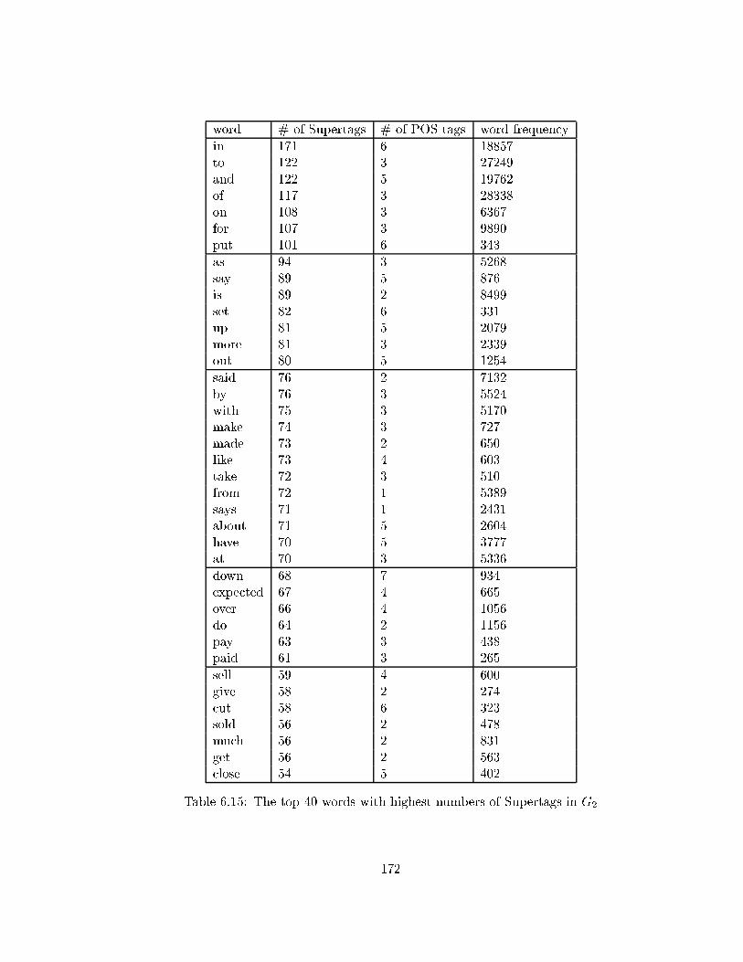
word # of Supertags # of POS tags word frequency
in 171 6 18857to 122 3 27249and 122 5 19762of 117 3 28338on 108 3 6367for 107 3 9890put 101 6 343
as 94 3 5268say 89 5 876is 89 2 8499set 82 6 331up 81 5 2079more 81 3 2339out 80 5 1254
said 76 2 7132by 76 3 5524with 75 3 5170make 74 3 727made 73 2 650like 73 4 603take 72 3 510from 72 1 5389says 71 1 2431about 71 5 2604have 70 5 3777at 70 3 5336
down 68 7 934expected 67 4 665over 66 4 1056do 64 2 1156pay 63 3 438paid 61 3 265
sell 59 4 600give 58 2 274cut 58 6 323sold 56 2 478much 56 2 831get 56 2 563close 54 5 402
Table 6.15: The top 40 words with highest numbers of Supertags in G2
172

discussed in Section 5.9.2.
To compare these three methods with respect to Supertagging, we use the data con-
verted by these methods to train a Supertagger. In the experiment, the Supertagger
(Srinivas, 1997), the evaluation tool, and the original PTB data are identical, but the con-
version algorithms and the data produced by the conversion algorithms are di�erent. The
results are given in Table 6.16.20 The results of Chen & Vijay's method come from their
paper (Chen and Vijay-Shanker, 2000). They built eight grammars. We list two of them
that seem to be most relevant: C4 uses a reduced tagset while C3 uses the PTB tagset. As
for Srinivas' results, we had to rerun his Supertagger using his data on the sections that
we have chosen, because his previous results were trained and tested on di�erent sections
of the PTB.21
We calculated two baselines for each set of data produced by the conversion algorithms.
For the �rst baseline, we tagged each word in testing data with the most common Supertag
with respect to that word in the training data. For an unknown word, the most common
Supertag was used. For the second baseline, we used a trigram POS tagger to tag the
20As usual, we use Sections 2-21 of the PTB for training and Section 22 or 23 for testing. We include
the results for Section 22 because (Chen and Vijay-Shanker, 2000) is tested on that section and its results
on Section 23 are not available.21Notably, the results we report on Srinivas' data, 85.78% on Section 23 and 85.53% on Section 22, are
lower than the 92.2% reported in (Srinivas, 1997), 91.37% in (Chen et al., 1999) and 88.0% in (Doran,
2000). There are several reasons for the di�erences. First, the size of training data in our experiment is
smaller than the one for his previous work, which was trained on Sections 0-24 except for Section 20 and
tested on Section 20. Second, we treat punctuation marks as normal words during evaluation because, like
other words, punctuation marks can anchor etrees, whereas he treated the Supertags for punctuation marks
as always correct. Third, he used some equivalence classes during evaluations. If a word is mis-tagged as
x, and its the correct Supertag is y, he did not consider that to be an error if x and y appeared in the
same equivalence class. We suspect that the reason that these Supertagging errors were disregarded is that
they might not a�ect parsing results when the Supertags are combined to form parse trees. For example,
both adjectives and nouns can modify other nouns. The two templates (i.e., Supertags) representing these
modi�cation relations look the same except for the POS tags of the anchors. If a word that should be
tagged with one Supertag is mis-tagged with the other Supertag, it is likely that the wrong Supertag can
still �t with other Supertags in the sentence to produce the correct parse tree. In our experiment, we did
not use these equivalence classes.
173
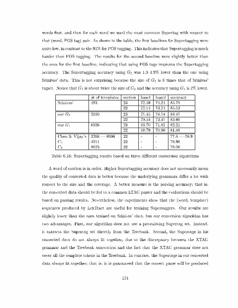
words �rst, and then for each word we used the most common Supertag with respect to
that (word, POS tag) pair. As shown in the table, the �rst baselines for Supertagging were
quite low, in contrast to the 91% for POS tagging. This indicates that Supertagging is much
harder than POS tagging. The results for the second baseline were slightly better than
the ones for the �rst baseline, indicating that using POS tags improves the Supertagging
accuracy. The Supertagging accuracy using G2 was 1.3{1.9% lower than the one using
Srinivas' data. This is not surprising because the size of G2 is 6 times that of Srinivas'
tagset. Notice that G1 is about twice the size of G2 and the accuracy using G1 is 2% lower.
# of templates section base1 base2 accuracy
Srinivas' 483 23 72.59 74.24 85.7822 72.14 73.74 85.53
our G2 2920 23 71.45 74.14 84.4122 70.54 73.41 83.60
our G1 6926 23 69.70 71.82 82.2122 68.79 70.90 81.88
Chen & Vijay's 2366 | 8996 22 - - 77.8 | 78.9C4 4911 22 - - 78.90C3 8623 22 - - 78.00
Table 6.16: Supertagging results based on three di�erent conversion algorithms
A word of caution is in order. Higher Supertagging accuracy does not necessarily mean
the quality of converted data is better because the underlying grammars di�er a lot with
respect to the size and the coverage. A better measure is the parsing accuracy; that is,
the converted data should be fed to a common LTAG parser and the evaluations should be
based on parsing results. Nevertheless, the experiments show that the (word, template)
sequences produced by LexTract are useful for training Supertaggers. Our results are
slightly lower than the ones trained on Srinivas' data, but our conversion algorithm has
two advantages. First, our algorithm does not use a pre-existing Supertag set. Instead,
it extracts the Supertag set directly from the Treebank. Second, the Supertags in his
converted data do not always �t together, due to the discrepancy between the XTAG
grammar and the Treebank annotation and the fact that the XTAG grammar does not
cover all the template tokens in the Treebank. In contrast, the Supertags in our converted
data always �t together; that is, it is guaranteed that the correct parse will be produced
174
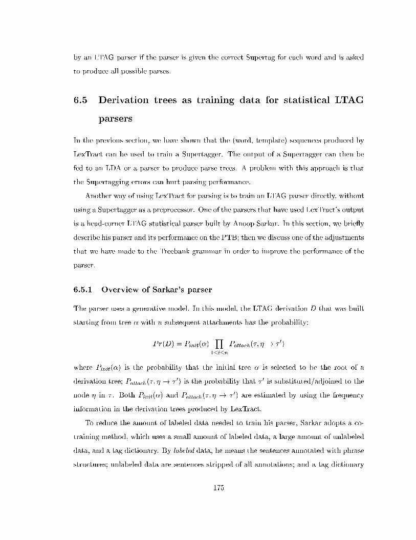
by an LTAG parser if the parser is given the correct Supertag for each word and is asked
to produce all possible parses.
6.5 Derivation trees as training data for statistical LTAG
parsers
In the previous section, we have shown that the (word, template) sequences produced by
LexTract can be used to train a Supertagger. The output of a Supertagger can then be
fed to an LDA or a parser to produce parse trees. A problem with this approach is that
the Supertagging errors can hurt parsing performance.
Another way of using LexTract for parsing is to train an LTAG parser directly, without
using a Supertagger as a preprocessor. One of the parsers that have used LexTract's output
is a head-corner LTAG statistical parser built by Anoop Sarkar. In this section, we brie y
describe his parser and its performance on the PTB; then we discuss one of the adjustments
that we have made to the Treebank grammar in order to improve the performance of the
parser.
6.5.1 Overview of Sarkar's parser
The parser uses a generative model. In this model, the LTAG derivation D that was built
starting from tree � with n subsequent attachments has the probability:
Pr(D) = Pinit(�)Y
1�i�n
Pattach(�; � ! � 0)
where Pinit(�) is the probability that the initial tree � is selected to be the root of a
derivation tree; Pattach(�; � ! � 0) is the probability that � 0 is substituted/adjoined to the
node � in � . Both Pinit(�) and Pattach(�; � ! � 0) are estimated by using the frequency
information in the derivation trees produced by LexTract.
To reduce the amount of labeled data needed to train his parser, Sarkar adopts a co-
training method, which uses a small amount of labeled data, a large amount of unlabeled
data, and a tag dictionary. By labeled data, he means the sentences annotated with phrase
structures; unlabeled data are sentences stripped of all annotations; and a tag dictionary
175

is a set of (word, template) pairs. In his experiment, the labeled data are Sections 02-06
of the PTB, the unlabeled data are Sections 07-21 stripped of all annotation, and the tag
dictionary includes all the (word, sequence) pairs from Sections 02-21. When tested on
Section 23 of the PTB, the labeled bracketing precision and recall are 80.02% and 79.64%,
respectively. Considering that the labeled data used by the parser are only about 25% of
the training data used by other parsers, we believe that the results are very promising.
The details of the generative model, the co-training method, and the experiment can be
found in (Sarkar, 2001).
6.5.2 Adjustments to the Treebank grammars for parsing
To create a Treebank grammar that is more suitable to parsing, we have made a few
adjustments to LexTract. In this section, we discuss one of them, which is to add insertion
markers to some nodes in fully bracketed ttrees and to the corresponding nodes in extracted
etrees. Let us explain why such tags are needed with an example. In Figure 6.15, to build
etrees, LexTract �rst fully brackets the phrase structure T1 in (a), then decomposes the
fully bracketed structure T2 in (b) into a set of etrees in (c). In the process, LexTract
inserts an extra node V P3 to T2, and the corresponding etree node for V P3:top is the foot
node of �1 in (c). If no insertion tags are used, when an LTAG parser uses the etrees
in (c) to parse the sentence John will come tomorrow, it will produce T2 as a parse tree,
rather than T1. When the parse tree T2 is compared with the original phrase structure in
the Treebank (which is T1), the precision is less than 100%. In other words, the parser is
punished for producing the fully bracketed structure. To avoid this, LexTract now adds
insertion tags to both V P3:top in T2 and the VP foot node of �1. Now when the parser
takes the same etrees in (c) but with this extra tag in the foot node of �1, it will produce
the same parse tree T2 but with the extra insertion tag in V P3:top. The parser can then
remove all the nodes in T2 whose top part has an insertion tag, resulting in the parse tree
T1.22
22LexTract inserts two types of nodes in the fully bracketed ttrees: one is for a modi�er that appears
outside the head and its arguments, as in this example; the other type is for a modi�er that appears between
the head and its arguments. For the �rst type, the insertion tag is added to the top part of the inserted
node in the fully bracketed ttree and to the corresponding node (which is the foot node of a mod-etree);
176
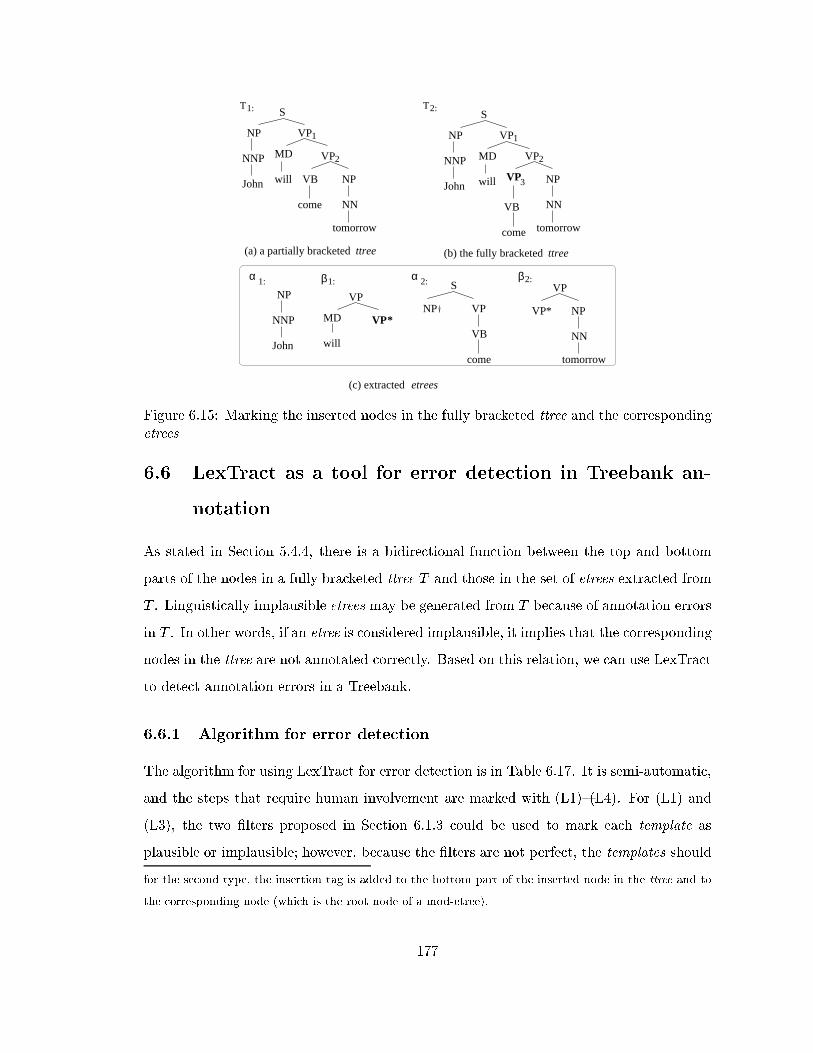
S
VPNNP
NP VP
John VB NP
NN
will
come
tomorrow
MD
NNP
NP
John
S
NP VP
VB
come
NP
NN
tomorrow
VP*
VPα 1: β2:
NNP
NP
John
ttree
etrees(c) extracted
(a) a partially bracketed ttree (b) the fully bracketed
VP
MD
will
VP*
S
VP
will
MD
3
2
1
VP
NP
NN
tomorrow
VP
come
VB
1
2
T T
β1: α 2:
1: 2:
Figure 6.15: Marking the inserted nodes in the fully bracketed ttree and the correspondingetrees
6.6 LexTract as a tool for error detection in Treebank an-
notation
As stated in Section 5.4.4, there is a bidirectional function between the top and bottom
parts of the nodes in a fully bracketed ttree T and those in the set of etrees extracted from
T . Linguistically implausible etrees may be generated from T because of annotation errors
in T . In other words, if an etree is considered implausible, it implies that the corresponding
nodes in the ttree are not annotated correctly. Based on this relation, we can use LexTract
to detect annotation errors in a Treebank.
6.6.1 Algorithm for error detection
The algorithm for using LexTract for error detection is in Table 6.17. It is semi-automatic,
and the steps that require human involvement are marked with (L1){(L4). For (L1) and
(L3), the two �lters proposed in Section 6.1.3 could be used to mark each template as
plausible or implausible; however, because the �lters are not perfect, the templates should
for the second type, the insertion tag is added to the bottom part of the inserted node in the ttree and to
the corresponding node (which is the root node of a mod-etree).
177

still be double checked by a linguistics expert. As for (L2) and (L4), the algorithm would
point out the nodes in ttrees that need to be checked, but it is up to the user of the tool
to decide what kind of modi�cation is needed to �x the errors in the ttree.
(A) run LexTract on the whole Treebank to generate a grammar G.(B) check each template in G and decide whether it is plausible or not. | (L1)
(C) for (each Treebank �le f)(C1) run LexTract to generate a grammar Gf ;(C2) for (each template ef 2 Gf )
if (9e 2 G, such that ef and e have the same structure)then if (e is marked as implausible in G)
then modify the ttree in f that generates ef ; | (L2)else
/* ef is a new template */check ef and decide whether it is plausible or not; | (L3)
add ef to G;if (ef is implausible)then modify the ttree in f that generates ef ; | (L4)
(C3) repeat (C1)-(C2) until Gf is a subset of G and Gf includesonly plausible templates;
Table 6.17: Algorithm for error detection
6.6.2 Types of error that LexTract detects
From the algorithm in Table 6.17, it is clear that annotation errors can be detected by
LexTract if and only if they result in implausible templates. These errors can be classi�ed
as follows:
� Formatting errors in ttrees such as unbalanced brackets and illegal tags: This type
of error can be totally avoided if the Treebank is built with proper annotation tools
(See Appendix B.7.2).23 When a ttree is not properly formatted, LexTract will give
a warning and exit without further processing of the ttree.
23For example, the English Penn Treebank uses a tool to add a left bracket and a right bracket in one
operation, so there should be no unbalanced brackets in that Treebank.
178

� Wrong syntactic labels (including POS tags, syntactic category tags and empty cat-
egory tags): Besides careless typos (e.g., using the tag LC (localizer) rather than CL
(classi�er) for a classi�er in the Chinese Treebank), wrong syntactic labels are often
due to incompatible labels at several levels. For example, in Chinese, a coordinat-
ing conjunction (CC) such as t�ong is also a preposition (IN); therefore, the sentence
\John t�ong/and with Mary z�ou/leave le/ASP" means either \John and Mary left"
or \John left with Mary", and both structures in Figure 6.16(a) and 6.16(b) are cor-
rect.24 However, the structure in Figure 6.16(c) is incorrect because the POS tag
CC and the syntactic category PP don't match, resulting in an implausible etree in
Figure 6.16(d). This type of error is relatively common because POS tagging and
bracketing are often done at separate annotation stages by di�erent annotators.
(c) the incompatible labels
(S (NP-SBJ (NNP John))(VP (PP (CC tong)
(NP (NNP Mary)))(VB zou)(AS le)))
VP
PP VP*
NPCC
tong
(d) the resulting etree
(b) tong as a preposition
(S (NP-SBJ (NNP John))(VP (PP (IN tong)
(NP (NNP Mary)))(VB zou)(AS le)))
(a) tong as a conjunction
(S (NP-SBJ (NP (NNP John))(CC tong)(NP (NNP Mary)))
(VP (VB zou)(AS le)))
Figure 6.16: An error caused by incompatible labels
� Wrong or missing function tags: LexTract uses syntactic labels and function tags to
24Because most of the readers are more familiar with the English Penn Treebank than the Chinese Penn
Treebank, in this example we adopt the annotation convention and the tagset that are used in the English
Penn Treebank (except for the tag AS for an aspect marker, which does not appear in the English tagset).
179
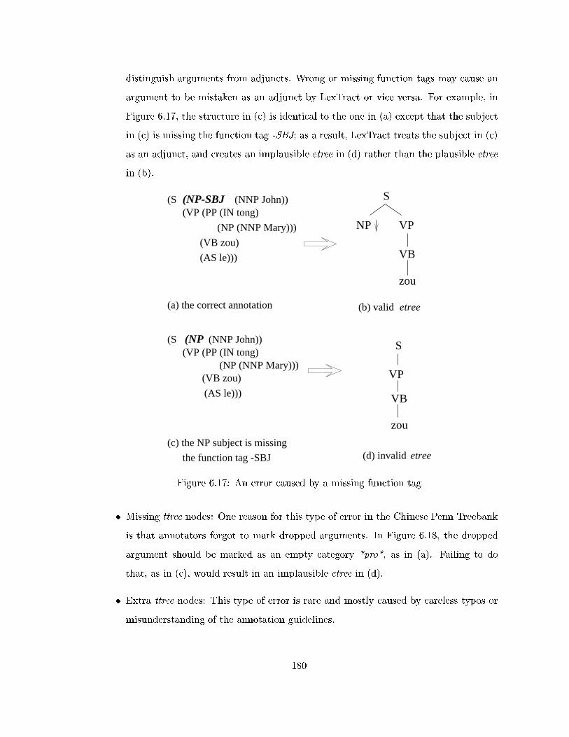
distinguish arguments from adjuncts. Wrong or missing function tags may cause an
argument to be mistaken as an adjunct by LexTract or vice versa. For example, in
Figure 6.17, the structure in (c) is identical to the one in (a) except that the subject
in (c) is missing the function tag -SBJ; as a result, LexTract treats the subject in (c)
as an adjunct, and creates an implausible etree in (d) rather than the plausible etree
in (b).
S
VB
VPNP
zou
VP
VB
zou
S
(d) invalid etree
(a) the correct annotation
(VP (PP (IN tong)
(NP (NNP Mary)))
(VB zou)
(AS le)))
(S (NP-SBJ (NNP John))
(NP(S(VP (PP (IN tong)
(NP (NNP Mary)))(VB zou)
(AS le)))
(NNP John))
(b) valid etree
(c) the NP subject is missing
the function tag -SBJ
Figure 6.17: An error caused by a missing function tag
� Missing ttree nodes: One reason for this type of error in the Chinese Penn Treebank
is that annotators forgot to mark dropped arguments. In Figure 6.18, the dropped
argument should be marked as an empty category *pro*, as in (a). Failing to do
that, as in (c), would result in an implausible etree in (d).
� Extra ttree nodes: This type of error is rare and mostly caused by careless typos or
misunderstanding of the annotation guidelines.
180

(VP (PP (IN tong)
(VB zou)
(AS le)))
(S
(c) the sentence missesthe subject node
VP
VB
zou
S
(d) invalid etree
(VP (PP (IN tong)
(NP (NNP Mary)))
(VB zou)
(AS le)))
(S (NP-SBJ (-NONE- *pro*))
(a) the correct annotation
(NP (NNP Mary)))
S
VB
VPNP
zou
*pro*
(b) valid etree
Figure 6.18: An error caused by a missing subject node
Two observations are in order. First, the main function of LexTract is extracting
LTAGs and building derivation trees to train LTAG parsers and Supertaggers. Error
detection is only a byproduct of the system. Consequently, there are errors that LexTract
cannot detect; namely, the errors that do not result in implausible etrees. For example, in
English, a PP can modify either an NP or a VP. Given a particular context, in general,
only one attachment makes sense. If the Treebank chooses the wrong attachment, LexTract
cannot detect that error.
The second observation is that using templates can detect more annotation errors than
using context-free rules. For example, in English either the subject or the object of a verb
can undergo wh-movement and leave a trace in its position, as shown in Figure 6.19(a)
and 6.19(b). But the subject and the object cannot be moved at the same time, as in
Figure 6.19(c). That is, the �rst two templates are plausible but the third template is
not. However, all three templates consist of the same set of context-free rules as in Figure
6.19(d), and all the context-free rules are plausible. Thus, the annotation errors that result
in the implausible template in Figure 6.19(c) can be detected if we use templates, rather
181

than context-free rules.
S
NP S
NP VP
V@ NPε
S
NP S
NP VP
ε
NPV@
S
NP S
NP VP
ε
NPε V@ NP -> ε
S -> NP S
S -> NP VP
VP -> V NP
(a) (b) (c) (d)
Figure 6.19: Three templates and corresponding context-free rules
6.6.3 Experimental results
We used LexTract for the �nal cleanup of the Chinese Penn Treebank. The Treebank
contains about 100 thousand words after word segmentation, and the average sentence
length is 23.8 words. Before LexTract was used for the �nal cleanup, each Treebank �le
had been manually checked at least twice and the annotation accuracy was already above
95%. More details on the Treebank can be found in Appendix B.
Before the �nal cleanup, the Treebank grammar Go contained 1245 etree templates. It
took a linguistics expert about 10 hours to manually examine all the templates in Go to
determine whether they were plausible. After that, it took another person (who was one
of the two annotators in the Chinese Treebank project) about 20 hours to run LexTract
and correct each Treebank �le. After the cleanup, 169 templates in the old grammar
disappeared, and 38 templates were added to the new grammar; so the new grammar has
1114 etree templates.
To report the number of errors found by LexTract, we could have classi�ed the errors
according to the types listed in Section 6.6.2, such as POS tagging errors, missing func-
tion tags, and so on. However, keeping such a record is time-consuming. Due to time
constraints, we did not do that. Instead, we automatically counted the number of word
tokens in the Treebank that anchored distinct templates before and after the cleanup. We
found 579 word tokens (which account for 0.58% of the total number of word tokens in the
Treebank) whose templates had changed after the cleanup. The di�erences may not be
huge, but considering the accuracy before running LexTract was already above 95% (see
182

Appendix B.6), the results of the �nal cleanup were satisfactory.
6.7 MC sets for testing the Tree-locality Hypothesis
In Section 5.6, we discussed our strategy for testing the Tree-locality Hypothesis. It has
three stages. First, LexTract �nds all the examples that seem to violate the hypothesis. We
call these examples \non-tree-local", or \non-local" for short. Second, we classify all the
non-local examples according to the underlying constructions (such as NP-extraposition).
Third, we determine whether each construction could become tree-local if an alternative
analysis for the construction were adopted. In this section, we report our experimental
results on the PTB.
6.7.1 Stage 1: Finding \non-local" examples
Section 5.6 gave an algorithm that �nds all the examples that seem to violate the Tree-
locality Hypothesis (see Table 4.8). We ran this algorithm on the PTB and found many
non-local examples. Table 6.18 lists the the numbers of tree sets with particular sizes.
A tree set, in this context, includes (1) the two etree templates e1 and e2 in which the
co-indexed constituents appear, and (2) the etree templates that connect e1 and e2 in
the derivation trees. Out of 3151 tree sets, 999 have more than three templates (i.e., the
templates for the gap and the �ller do not adjoin to the same template), and they account
for 8.7% of all the occurrences of tree sets.
size of tree sets � 3 (tree-local sets) 4 5 6 7 8 subtotal total
types 2152(68.3%) 874 94 26 4 1 999(31.7%) 3151
tokens 19994(91.3%) 1772 102 26 4 1 1905(8.7%) 21899
Table 6.18: Numbers of tree sets and their frequencies in the PTB
6.7.2 Stage 2: Classifying \non-local" examples
We have manually classi�ed the \non-local" examples found in Stage 1. The results are
given in Table 6.19. Among the 999 sets, 71 are caused by obvious annotation errors, 65 are
183

tree-local but our extraction algorithm does not recognize that.25 For the remaining ones,
we divide them into seven classes according to the underlying syntactic constructions.26
PTB LexTract NP- extraction it- comparative of-PP paren- so .. otherserrors errors EXP from coord. EXP construction thetical that
71 65 337 209 176 50 31 30 11 19
Table 6.19: Classi�cation of 999 MC sets that look non-tree-local
An example for each construction is given in (1) | (7). According to the Treebank an-
notation, every sentence except (2) has an empty category "i, which modi�es a constituent
Y P (in boldface) and is co-indexed with another constituent XP .27 Figures 6.20 to 6.26
show the simpli�ed Treebank annotation for these sentences and the corresponding etree
sets which include the etrees for "i, etrees for XP , and other etrees that connect them in
the derivation tree. The arrows in the �gures mark the positions of the empty categories
and the XPs that co-indexed with the empty categories.
(1) NP-extraposition:
Supply troubles were on the minds of Treasury investors "i yesterday, [who
worried about the ood]i.
(2) Extraction from coordinated phrases:
His departure was nothing [that]i we desired "i or worked for "i.
(3) It-extraposition:
It "i is too early [to say whether that will happen]i.
25The reason for the LexTract errors is that LexTract does not factor out predicative auxiliary trees
(such as the one for \think") in a relative clause, as discussed in Section 5.8.4.
26We also use an additional class for 19 examples that belong to a number of uncommon constructions.27All the examples come from the PTB. The treebank has 10 tags for empty categories. For example,
it uses *EXP* for the empty categories in the it-extraposition, *T* in the NP-extraposition, of-PP, and
parenthetical, and *ICH* in extraction from coordinated phrases, comparative construction, and so ... that
construction. For the sake of uniformity, in (1) | (7) and Figures 6.20 to 6.26, we use "i for all empty
categories.
184

Supply troubles
NP
S
VP
VBD
were IN
on
the minds IN
of NP
NP
PP
yesterday
NP
who worried
SBAR
Treasury investors
SBAR
NP
εi
i
NP PPabout the flood
NP
NNS
investors
α3:
β1:
NP
NP
NP PP
of
*
IN
NP
NNS
minds
α2:
α 1: VP
IN
on
NP
PP
S
NP
*
i
NP
NP SBAR
ε
β2:
*
β3:
VP SBAR i
VP
NP
worried
VBD
VP
SWHNP
ε
(a) (b)
Figure 6.20: An example of the NP-extraposition construction
(4) Comparative construction:
Federal Express goes further "i in this respect [than any company that I know
of]i.
(5) Of-PP:
[Of all the ethnic tensions in America]i, which "i is the most troublesome right
now?
(6) Parenthetical:
[He spends most weekends ying his helicopter to one of his nine courses, he said
"i, two of which were designed by Jack Nicklaus.]i
(7) So ... that construction:
The opposition parties are so often "i opposed to whatever LDP does [that it
would be a waste of time]i.
6.7.3 Stage 3: Studying \non-local" constructions
In the treebank, in addition to marking syntactic movement, empty categories and reference
indexes are also used to indicate where a constituent should be interpreted. If a constituent
185
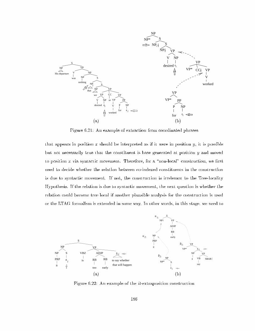
εi
NP
His departure
S
VP
V
was
nothing
NP
NP
S
NP
we VP
desired
V NP
CC
or PP
VP
VP
S
P NP
for ε i
NPi
worked
VP
V
that
CC
VP
VP
V
worked
VP*
εi
VP
VP* PP
P NP
for
εi
NP*
NP
S
S
NP
V
VP
desired
NP
NPi
(a) (b)
Figure 6.21: An example of extraction from coordinated phrases
that appears in position x should be interpreted as if it were in position y, it is possible
but not necessarily true that the constituent is base generated at position y and moved
to position x via syntactic movement. Therefore, for a \non-local" construction, we �rst
need to decide whether the relation between co-indexed constituents in the construction
is due to syntactic movement. If not, the construction is irrelevant to the Tree-locality
Hypothesis. If the relation is due to syntactic movement, the next question is whether the
relation could become tree-local if another plausible analysis for the construction is used
or the LTAG formalism is extended in some way. In other words, in this stage, we need to
NP
S
VP
ADJP S
is
VBZ
RB RB
it
PRP
NP
ε
S
to say whether
that will happentoo early
i
i
NP
PRP
itVP
VP* S
VP
ε
NP
say
VB SBAR
i
NP
NP* S
ε i
β2:
α 2:
α1:
β1:
ADJP
RB
early
S
VPNP
(a) (b)
Figure 6.22: An example of the it-extraposition construction
186
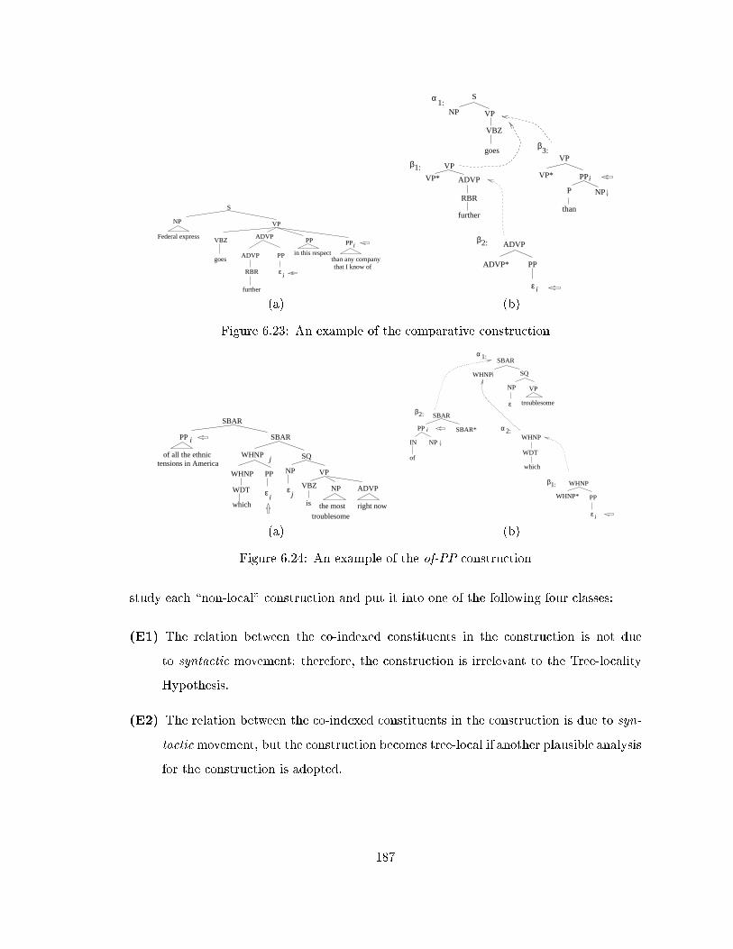
Federal express
S
NP
ADVPVBZ
goes
PP
in this respectthan any companythat I know of
PP
further
RBR
ADVP
ε
PP
i
i
VP
VP*
VP
PP
NPP
than
β3:
i
ADVP* PP
ADVP
ε
β2:
i
NP VP
VBZ
goes
Sα1:
VP
VP* ADVP
RBR
further
β1:
(a) (b)
Figure 6.23: An example of the comparative construction
PP SBAR
SQ
NP VP
VBZ NP
SBAR
of all the ethnic
WHNP
WDT
which
PP
WHNP
ADVP
right nowisε
iε
j
tensions in America
i
j
troublesomethe most
SBAR
SQ
NP VP
troublesomeε
WHNP
WHNP
WHNP*
ε
PP
β1:
WHNP
WDT
which
α 2:
α 1:
i
β2: SBAR
IN
SBAR*PP
NP
of
i
(a) (b)
Figure 6.24: An example of the of-PP construction
study each \non-local" construction and put it into one of the following four classes:
(E1) The relation between the co-indexed constituents in the construction is not due
to syntactic movement; therefore, the construction is irrelevant to the Tree-locality
Hypothesis.
(E2) The relation between the co-indexed constituents in the construction is due to syn-
tacticmovement, but the construction becomes tree-local if another plausible analysis
for the construction is adopted.
187

VBZ
spends
NP
S
mostweekends
S
NP VP
VBG NPεPP
IN
to
NP
NP
one
PP
IN
of
NP
PRN
VP
S
ε
i
isays
VP
SBAR
two of whichwere designedby Jack Nicklaus
NP
NP
he
VBZPRP
flyinghis
helicopter
He
NP
his ninecourses
α2: SNP VP
VBG
flying
NP
PP
IN
to
NP
VP
VP*
β1:
S
VP
SNPVBZ
spends
NP
α 1:
NP
CD
one
α3:
of
NP
NP* PP
IN NP
β2:
NP
NNS
courses
α 4:
β3:
NP
NP* PRN
NP VP
VBZ S
εsays
i
i
(a) (b)
Figure 6.25: An example of the parenthetical construction
The opposition
S
NP
ADVPVBP
ADVP
εi
VP
parties
are SBAR
ADJP
opposed to that it wouldbe a waste of time
whateverLDP doesso often
SBAR i
S
NP VP
waste
NP VP
Sα1:
opposed
VP
VP*
ADVP*
ADVP
ε
β1:
β2:
SBAR
i
ADVP
RB
often
VP*
VP
β3:
SBAR
IN
i
(a) (b)
Figure 6.26: An example of the so ... that construction
(E3) The relation between the co-indexed constituents in the construction is due to syn-
tactic movement, but the construction becomes tree-local if the de�nitions of substi-
tution and adjoining operations in the LTAG formalism are modi�ed. Some recent
work on modifying these de�nitions to account for certain syntactic movement can
be found in (Joshi and Vijay-Shanker, 1999; Kulick, 2000).
(E4) The relation between the co-indexed constituents in the construction is due to syn-
tactic movement, and the construction is truly non-local. Therefore, the construction
is a counter-example to the Tree-locality Hypothesis.
For some of the constructions in Section 6.7.2 (such as NP-extraposition), there is no
consensus in the linguistics community on their treatments. Providing good analyses for
them requires linguistic expertise, and is beyond the scope of this thesis. Nevertheless, we
188
want to point out that for each construction there is strong evidence to support the view
that the relation between the co-indexed constituents is not due to syntactic movement.
For instance, in (Xia and Bleam, 2000), we argued that one type of extraposed phrase in
the NP-extraposition construction is anaphoric in the sense that the dependency is not
represented in the syntax or in the semantics (such as in the synchronous TAG analysis
given in (Abeill�e, 1994)). Rather, a process more like pronoun resolution should be applied
in a pragmatic component to determine the nature of the dependency.
In summary, the Tree-locality Hypothesis is an important hypothesis in the LTAG
formalism and is relevant to linguistic theories in general; therefore, it should be thoroughly
tested. The method that we propose to test the hypothesis with naturally-occuring data
has three steps: �nding non-local examples in the data, classifying non-local examples
according to the underlying constructions, and studying the non-local constructions and
deciding whether the examples are genuine counter-examples to the hypothesis. LexTract
enables us to automate the �rst step; that is, it can automatically extract all the non-local
examples from Treebanks.
6.8 Summary
In this chapter, we have discussed four types of applications for LexTract. First, Treebank
grammars produced by LexTract are useful for grammar development and comparison.
For example, a Treebank grammar can be used as a stand-alone grammar. We also used a
Treebank grammar extracted from the English Penn Treebank to estimate and improve the
coverage of the XTAG grammar. In addition, we have compared Treebank grammars for
English, Chinese, and Korean, and shown that the majority of the core grammar structures
for these three languages are easily inter-mappable. Second, the Treebank grammar and
derivation trees produced by LexTract were used to train a Supertagger and a statistical
LTAG parser with satisfactory results. Third, we have used LexTract to detect annotation
errors in the Chinese Penn Treebank. Last, we have used LexTract to �nd all the non-
local examples from the English Penn Treebank. These examples should be examined to
determine whether they are counter-examples to the Tree-locality Hypothesis. All these
189

applications indicate that LexTract is not only an engineering tool of great value, but it is
also very useful for investigating theoretical linguistics.
190

Chapter 7
Phrase structures and dependency
structures
Treebanks are of two types according to their annotation schemata: phrase-structure Tree-
banks such as the English Penn Treebank (Marcus et al., 1993) and dependency Treebanks
such as the Czech dependency Treebank (Haji�c, 1998). In Chapters 5 and 6, we have run
LexTract on phrase-structure Treebanks. In this chapter, we address the following ques-
tions:
� What's the relationship between phrase structures and dependency structures?
� Can LexTract run on a dependency Treebank?
Long before Treebanks were developed and widely used for natural language process-
ing, there had been much discussion of comparison between dependency grammars and
context-free phrase-structure grammars. For instance, Gaifman (1965) shows that depen-
dency grammars and context-free grammars (CFGs) are weakly equivalent, and depen-
dency grammars are strongly equivalent to a subclass of CFGs. In this chapter, we address
the relationship between dependency structures and phrase structures from a practical per-
spective; namely, we want to explore di�erent algorithms that convert between dependency
structures and phrase structures, and to determine what information should be present in
the structures to facilitate the conversion.
191

The chapter is organized as follows. In Section 7.1, we discuss a particular representa-
tion for dependency structures, which we choose to use in this chapter. In Section 7.2, we
give an algorithm that converts phrase structures to dependency structures. In Section 7.3,
we propose a new algorithm that converts dependency structures into phrase structures,
and compare it with two existing algorithms. In Section 7.4, we evaluate the performance
of the three algorithms in Section 7.3 using an existing phrase-structure Treebank. In
Section 7.5, we argue that the inclusion of empty categories in dependency structures will
simplify the conversion between the two representations. We also give an algorithm that
builds grammars and derivation trees from dependency Treebanks directly.
7.1 Dependency structures
There is much variety of the representation of dependency structures. Figures 7.1 and 7.2
show two common representations. In the �rst representation, heads are connected to their
dependents by downward-sloping lines. In the second one (we call it a dependency tree,
or d-tree for short), heads are parents of their dependents in a tree. If a d-tree is ordered
(that is, the dependents of the same head are ordered according to their positions in the
sentence) and the sentence is projective,1 then traversing a d-tree will yield the correct
word order of the sentence and therefore the two representations are equivalent. In this
chapter, we use the second representation because of its close resemblance to the derivation
trees in the LTAG formalism. We further assume that a d-tree is ordered. In addition to
the dependency links, a d-tree may also include other information such as Part-of-Speech
Tags for words and the type of dependency links (argument, modi�er, and so on).
Another variation in the representation of dependency structures is on the treatment of
empty categories. Empty categories (such as traces) are often used in phrase structures for
syntactic movement, dropped arguments, and so on. For example, in Figure 7.3, the empty
category � is coindexed with the WHNP which to mark the wh-movement. The sentence
is not projective because the wh-word who depends on the verb win, but the word believe
(which appears between who and win) does not directly or indirectly depend on win. Figure
1A sentence w1w2:::wn is projective if the following holds: for any pair of words (wi; wj), if wi depends
on wj , then any word between wi and wj in the sentence directly or indirectly depends on wj .
192
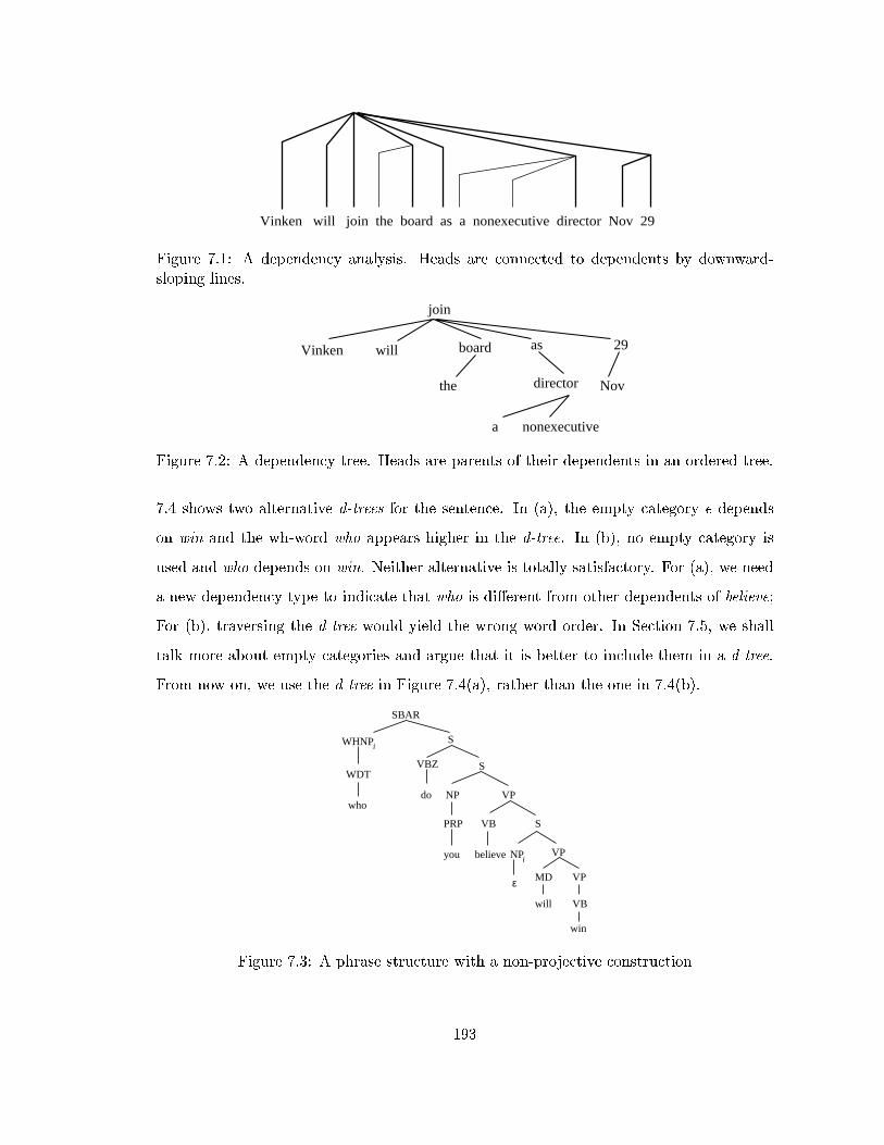
Vinken will join the board as a nonexecutive director Nov 29
Figure 7.1: A dependency analysis. Heads are connected to dependents by downward-sloping lines.
join
willVinken
nonexecutivea
board as
the
29
Novdirector
Figure 7.2: A dependency tree. Heads are parents of their dependents in an ordered tree.
7.4 shows two alternative d-trees for the sentence. In (a), the empty category � depends
on win and the wh-word who appears higher in the d-tree. In (b), no empty category is
used and who depends on win. Neither alternative is totally satisfactory. For (a), we need
a new dependency type to indicate that who is di�erent from other dependents of believe;
For (b), traversing the d-tree would yield the wrong word order. In Section 7.5, we shall
talk more about empty categories and argue that it is better to include them in a d-tree.
From now on, we use the d-tree in Figure 7.4(a), rather than the one in 7.4(b).
NP VP
MD VP
will VB
win
ε
NP VP
PRP
you
VB
believe
S
S
WHNP
SBAR
S
VBZ
do
WDT
who
i
i
Figure 7.3: A phrase structure with a non-projective construction
193

do you win
willwho
believe
who do you
willε
win
believe
(a) a d-tree that uses an empty category (b) a d-tree that does not use empty categories
Figure 7.4: Two alternative d-trees for the sentence in Figure 7.3
7.2 Converting phrase structures to dependency structures
The notion of head is important in both phrase structures and dependency structures. In
many linguistic theories such as X-bar theory and GB theory, each phrase structure has
a head that determines the main properties of the phrase and a head has several levels
of projections; whereas in a dependency structure the head is linked to its dependents.
In practice, the head information is explicitly marked in a dependency Treebank, but not
always so in a phrase-structure Treebank. A common way to �nd the head in a phrase
structure is to use a head percolation table (Magerman, 1995; Collins, 1997), as discussed
in Sections 5.3.1 and 5.4.1. For example, the entry (S right S/VP) in the head percolation
table says that the head-child2 of an S node is the �rst child of the node from the right
with the label S or VP.
Once the heads in phrase structures are found, the conversion from phrase structures
to dependency structures is straightforward, as shown below:
(a) Mark the head-child of each node in a phrase structure, using the head percolation
table (see Section 5.4.1).
(b) In the dependency structure, make the head of each non-head-child depend on the
head of the head-child.
Figure 7.5 shows a phrase structure in the English Penn Treebank (Marcus et al., 1993).
In addition to the syntactic labels (such as NP for a noun phrase), the Treebank also uses
function tags (such as SBJ for the subject) for grammatical functions. In this phrase
2The head-child of a node XP is the child of the node XP that is the ancestor of the head of the XP in
the phrase structure.
194
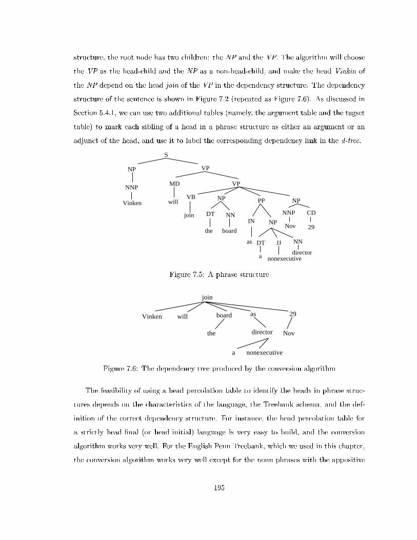
structure, the root node has two children: the NP and the VP. The algorithm will choose
the VP as the head-child and the NP as a non-head-child, and make the head Vinkin of
the NP depend on the head join of the VP in the dependency structure. The dependency
structure of the sentence is shown in Figure 7.2 (repeated as Figure 7.6). As discussed in
Section 5.4.1, we can use two additional tables (namely, the argument table and the tagset
table) to mark each sibling of a head in a phrase structure as either an argument or an
adjunct of the head, and use it to label the corresponding dependency link in the d-tree.
NP
S
VP
NNP
Vinken
MD
will
VP
PP NPVB
join
NP
DT NN
the board
as JJ
IN NP
NNP CD
29Nov
DT NN
nonexecutivedirector
a
Figure 7.5: A phrase structure
join
willVinken
nonexecutivea
board as
the
29
Novdirector
Figure 7.6: The dependency tree produced by the conversion algorithm
The feasibility of using a head percolation table to identify the heads in phrase struc-
tures depends on the characteristics of the language, the Treebank schema, and the def-
inition of the correct dependency structure. For instance, the head percolation table for
a strictly head-�nal (or head-initial) language is very easy to build, and the conversion
algorithm works very well. For the English Penn Treebank, which we used in this chapter,
the conversion algorithm works very well except for the noun phrases with the appositive
195

construction. For example, the conversion algorithm would choose the appositive \the
CEO of FNX" as the head child of the phrase \John Smith, the CEO of FNX", whereas
the correct head child should be \John Smith".
7.3 Converting dependency structures to phrase structures
The main information that is present in phrase structures but not in dependency structures
is the type of syntactic category (e.g., NP, VP, and S); therefore, to recover syntactic
categories, any algorithm that converts dependency structures to phrase structures needs
to address the following questions:
Projections for each category: for a category X, what kind of projections can X have?
Projection levels for dependents: Given a category Y depends on a category X in a
dependency structure, how far should Y project before it attaches to X's projection?
Attachment positions: Given a category Y depends on a category X in a dependency
structure, to what position on X's projection chain should Y's projection attach?
In this section, we discuss three conversion algorithms, each of which gives di�erent
answers to these three questions. To make the comparison easy, we shall apply each
algorithm to the d-tree in Figure 7.6 and compare the output of the algorithm with the
phrase structure for that sentence in the English Penn Treebank, as in Figure 7.5.
Evaluating these algorithms is tricky because just like dependency structures there is
often no consensus on what the correct phrase structure for a sentence should be. In this
chapter, we measure the performance of the algorithms by comparing their output with an
existing phrase-structure Treebank (namely, the English Penn Treebank) because of the
following reasons. First, the Treebank is available to the public, and provides an objective
although imperfect standard. Second, one goal of the conversion algorithms is to make it
possible to compare the performance of parsers that produce dependency structures with
the ones that produce phrase structures. Because most state-of-the-art phrase-structure
parsers are evaluated against an existing Treebank, we want to evaluate the conversion
algorithms in the same way. Third, a potential application of the conversion algorithms
196

is to help construct a phrase-structure Treebank for one language, given parallel corpora
and the phrase structures in the other language. One way to evaluate the quality of the
resulting Treebank is to compare it with an existing Treebank.
7.3.1 Algorithm 1
According to X-bar theory, a category X projects to X', which further projects to XP.
There are three types of rules, as shown in Figure 7.7(a).
(1) XP -> YP X’
(2) X’ -> X’ WP
(3) X’ -> X ZPY
(Spec)
XP
X’
X’
X
YP(Spec)
ZP(Arg)
WP(Mod)
(c) phrase structure(b) d-tree(a) rules in X-bar theory
W(Mod)
Z(Arg)
X
Figure 7.7: Rules in X-bar theory and the algorithm that is based on it
Algorithm 1, as adopted in (Covington, 1994b; Covington, 1994a), strictly follows X-
bar theory and uses the following heuristic rules to build phrase structures.
Two levels of projections for any head: X has two levels of projection: X' and XP
Maximal projections for dependents: If Y depends on X, it is always Y's maximal
projection YP that attaches to X's projection.
Fixed positions of attachment according to dependency types: If Y depends on
X, YP attaches to the head X's projection according to the dependency type:
� If Y is an argument of X, YP is a sister of X;
� If Y is a modi�er of X, YP adjoins to X';
� If Y is a speci�er of X, YP is a sister of X' and a child of XP.
The algorithm requires a d-tree to distinguish three types of dependents. If a head has
multiple modi�ers, the algorithm can assume that either a single X' or stacked X' is used.
The algorithm converts the d-tree in Figure 7.7(b) to the phrase structure in Figure 7.7(c).
197

Figure 7.8 shows the phrase structure for the d-tree in Figure 7.6, where the algorithm
uses single X' for multiple modi�ers of the same head.3
VP
V’
MD
will
VB
join
NP
Vinken
NNP
N’ PP
P’
IN
as
NP
V’
nonexecutive
VP
N’
Nov
NNP
N’
NP
N’
NP
CD
29ADJP
JJ
ADJ’
N’
NN
director
N’
V’
board
N’
NN
NP
DT
DT’
DTP
the
a
DT
DT’
DTP
Figure 7.8: The phrase structure built by algorithm 1 for the d-tree in Figure 7.6
7.3.2 Algorithm 2
Algorithm 2, as adopted by Collins and his colleagues (1999) when they converted the
Czech dependency Treebank (Haji�c, 1998) into a phrase-structure Treebank, produces a
phrase structure that is as at as possible. It uses the following heuristic rules to build
phrase structures:
One level of projection for any head: X has only one level of projection: XP.
Minimal projection for dependents: A dependent Y does not project to Y P unless
it has its own dependents.
Fixed position of attachment: A dependent is a sister of its head in the phrase struc-
ture.4
The algorithm treats all kinds of dependents equally. It converts the pattern in Figure
7.9(a) to the phrase structure in Figure 7.9(b). Notice that in Figure 7.9(b), Y does not3To make the phrase structure more readable, we use N' and NP as the X' and XP for all kinds of POS
tags for nouns (e.g., NNP, NN, and CD). Verbs and adjectives are treated similarly.4If a dependent Y has its own dependents, it projects to YP and YP is a sister of the head X; otherwise,
Y is a sister of the head X.
198
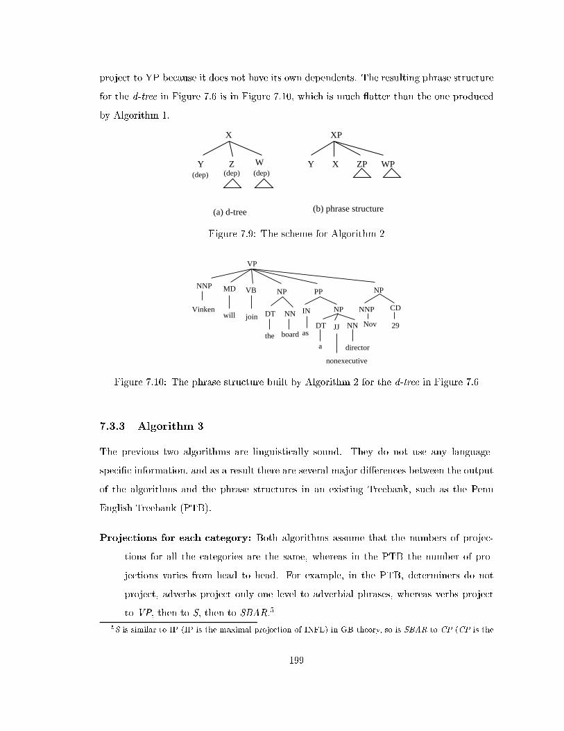
project to YP because it does not have its own dependents. The resulting phrase structure
for the d-tree in Figure 7.6 is in Figure 7.10, which is much atter than the one produced
by Algorithm 1.
Y W
XP
(dep) (dep) (dep)Z
X
(a) d-tree (b) phrase structure
X ZP WPY
Figure 7.9: The scheme for Algorithm 2
VP
VB
join
MD NP
DT
PP
IN
nonexecutive
NP
NNP CD
Nov 29
NP
NNJJDTthe
NN
board as
directora
will
NNP
Vinken
Figure 7.10: The phrase structure built by Algorithm 2 for the d-tree in Figure 7.6
7.3.3 Algorithm 3
The previous two algorithms are linguistically sound. They do not use any language-
speci�c information, and as a result there are several major di�erences between the output
of the algorithms and the phrase structures in an existing Treebank, such as the Penn
English Treebank (PTB).
Projections for each category: Both algorithms assume that the numbers of projec-
tions for all the categories are the same, whereas in the PTB the number of pro-
jections varies from head to head. For example, in the PTB, determiners do not
project, adverbs project only one level to adverbial phrases, whereas verbs project
to VP, then to S, then to SBAR.5
5S is similar to IP (IP is the maximal projection of INFL) in GB theory, so is SBAR to CP (CP is the
199
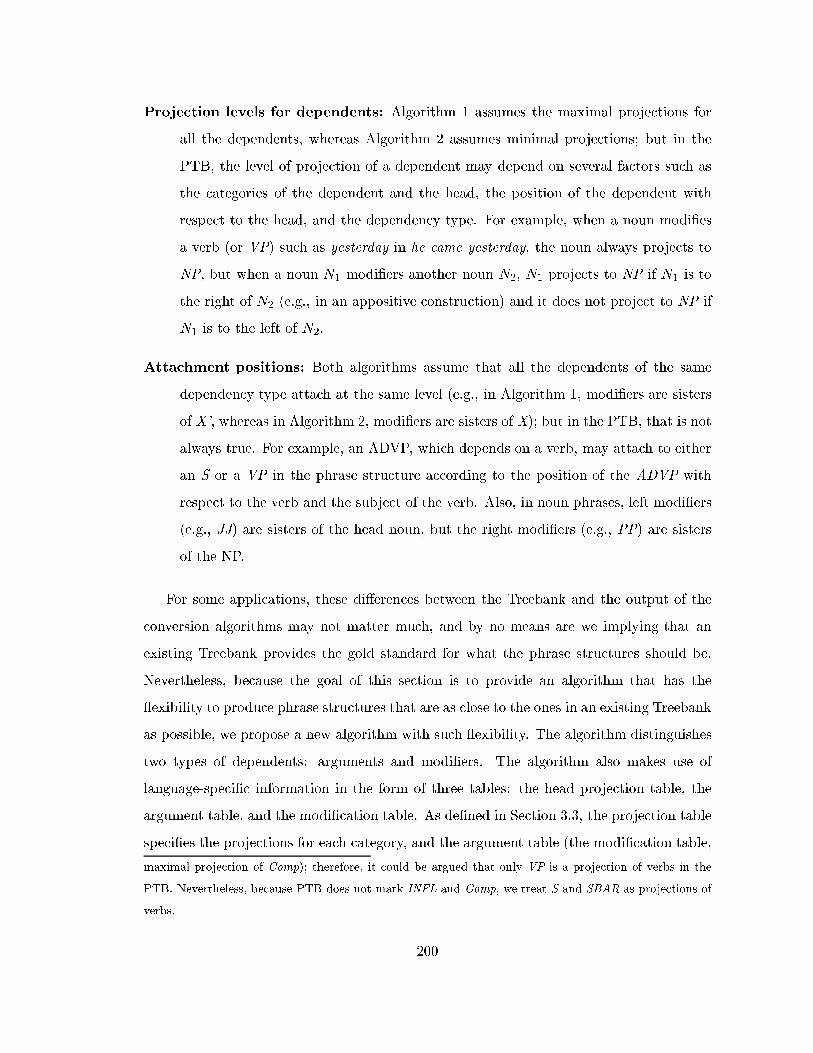
Projection levels for dependents: Algorithm 1 assumes the maximal projections for
all the dependents, whereas Algorithm 2 assumes minimal projections; but in the
PTB, the level of projection of a dependent may depend on several factors such as
the categories of the dependent and the head, the position of the dependent with
respect to the head, and the dependency type. For example, when a noun modi�es
a verb (or VP) such as yesterday in he came yesterday, the noun always projects to
NP, but when a noun N1 modi�ers another noun N2, N1 projects to NP if N1 is to
the right of N2 (e.g., in an appositive construction) and it does not project to NP if
N1 is to the left of N2.
Attachment positions: Both algorithms assume that all the dependents of the same
dependency type attach at the same level (e.g., in Algorithm 1, modi�ers are sisters
of X', whereas in Algorithm 2, modi�ers are sisters of X); but in the PTB, that is not
always true. For example, an ADVP, which depends on a verb, may attach to either
an S or a VP in the phrase structure according to the position of the ADVP with
respect to the verb and the subject of the verb. Also, in noun phrases, left modi�ers
(e.g., JJ) are sisters of the head noun, but the right modi�ers (e.g., PP) are sisters
of the NP.
For some applications, these di�erences between the Treebank and the output of the
conversion algorithms may not matter much, and by no means are we implying that an
existing Treebank provides the gold standard for what the phrase structures should be.
Nevertheless, because the goal of this section is to provide an algorithm that has the
exibility to produce phrase structures that are as close to the ones in an existing Treebank
as possible, we propose a new algorithm with such exibility. The algorithm distinguishes
two types of dependents: arguments and modi�ers. The algorithm also makes use of
language-speci�c information in the form of three tables: the head projection table, the
argument table, and the modi�cation table. As de�ned in Section 3.3, the projection table
speci�es the projections for each category, and the argument table (the modi�cation table,
maximal projection of Comp); therefore, it could be argued that only VP is a projection of verbs in the
PTB. Nevertheless, because PTB does not mark INFL and Comp, we treat S and SBAR as projections of
verbs.
200
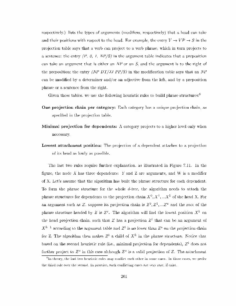
respectively.) lists the types of arguments (modi�ers, respectively) that a head can take
and their positions with respect to the head. For example, the entry V ! V P ! S in the
projection table says that a verb can project to a verb phrase, which in turn projects to
a sentence; the entry (P, 0, 1, NP/S) in the argument table indicates that a preposition
can take an argument that is either an NP or an S, and the argument is to the right of
the preposition; the entry (NP DT/JJ PP/S) in the modi�cation table says that an NP
can be modi�ed by a determiner and/or an adjective from the left, and by a preposition
phrase or a sentence from the right.
Given these tables, we use the following heuristic rules to build phrase structures:6
One projection chain per category: Each category has a unique projection chain, as
speci�ed in the projection table.
Minimal projection for dependents: A category projects to a higher level only when
necessary.
Lowest attachment position: The projection of a dependent attaches to a projection
of its head as lowly as possible.
The last two rules require further explanation, as illustrated in Figure 7.11. In the
�gure, the node X has three dependents: Y and Z are arguments, and W is a modi�er
of X. Let's assume that the algorithm has built the phrase structure for each dependent.
To form the phrase structure for the whole d-tree, the algorithm needs to attach the
phrase structures for dependents to the projection chain X0;X1; :::Xk of the head X. For
an argument such as Z, suppose its projection chain is Z0; Z1; :::Zu and the root of the
phrase structure headed by Z is Zs. The algorithm will �nd the lowest position Xh on
the head projection chain, such that Z has a projection Zt that can be an argument of
Xh�1 according to the argument table and Zt is no lower than Zs on the projection chain
for Z. The algorithm then makes Zt a child of Xh in the phrase structure. Notice that
based on the second heuristic rule (i.e., minimal projection for dependents), Zt does not
further project to Zu in this case although Zu is a valid projection of Z. The attachment6In theory, the last two heuristic rules may con ict each other in some cases. In those cases, we prefer
the third rule over the second. In practice, such con icting cases are very rare, if exist.
201

for modi�ers is similar except that the algorithm uses the modi�cation table instead of the
argument table.7
Z
X
Y W(Arg) (Arg) (Mod)
k
0
j
j-1
h
l
m
n
W
W
W
W00
h-1
X
X
X
X
X
X
Y
X i
Y
Y
Y
q
Z
Z
0
P
r
s
Zt
Zu
(b) phrase structure(a) d-tree
Figure 7.11: The scheme for Algorithm 3
The algorithm is in Table 7.1 and 7.2. We use a variable low visib index to store the
position of the lowest visible node on the chain; that is, the lowest node on the head chain
that the following dependents can attach to. The value of the variable is updated every
time a new dependent is attached to the head (see steps (E) and (G) in Table 7.1 and step
(F) in Table 7.2). We use another variable root index to store the position of the current
root of the phrase structure. Both variables start from 0 (i.e., the index of the head word
is 0).
The phrase structure produced by Algorithm 3 for the d-tree in Figure 7.6 is in Figure
7.12. In Figure 7.12, (a)-(e) are the phrase structures for �ve dependents of the head
join; (f) is the projection chain for the head. The arrows indicate the positions of the
attachment. Notice that to attach (a) to (f), the NNP Vinken needs to further project to
NP because according to the argument table, VP can take an NP, but not an NNP, as its
argument.
Algorithm 3 has been extended to handle two types of modi�ers, punctuation marks
and conjunctions. The extended algorithm is shown in Table 7.6:
7Note that once Zt becomes a child of Xh, other dependents of X (such as W) that are on the same
side as Z but are further away from X can attach only to Xh or higher on the projection chain of X.
202
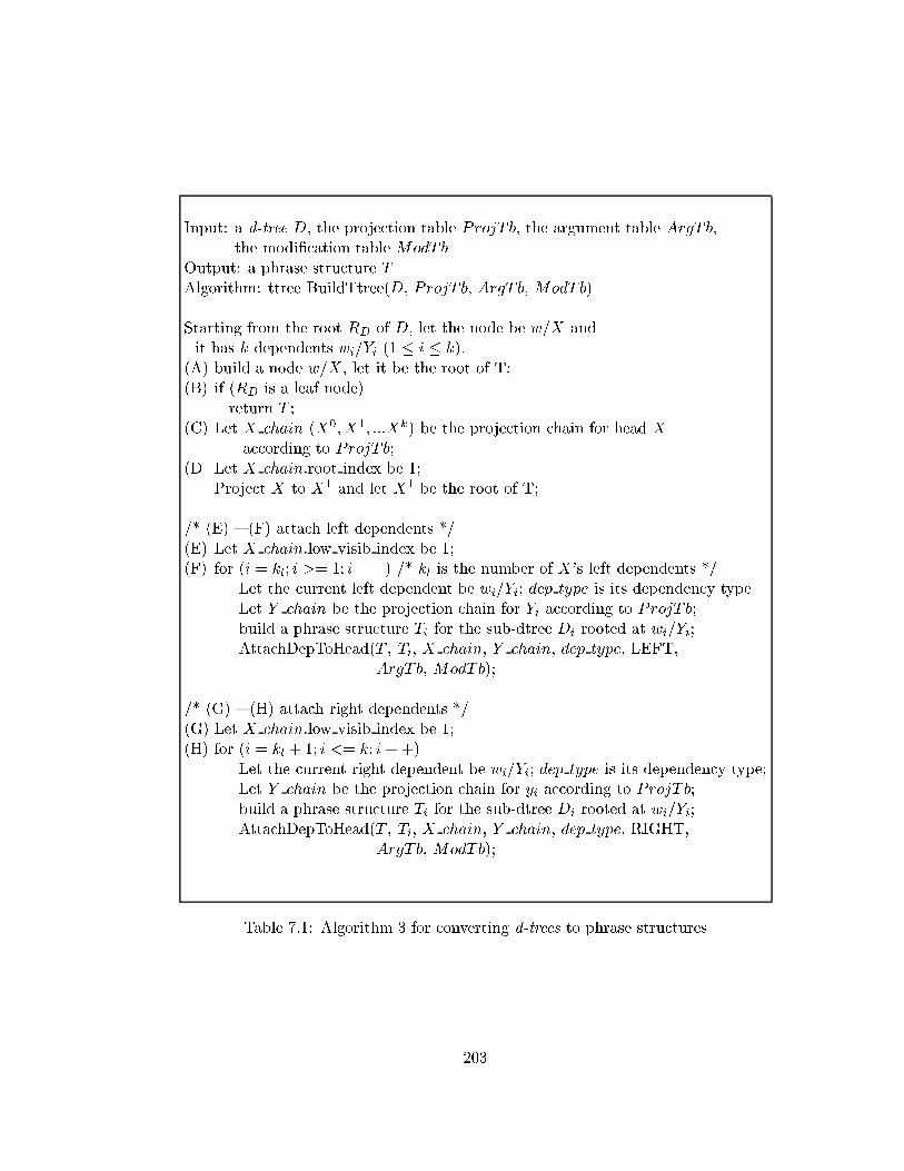
Input: a d-tree D, the projection table ProjT b, the argument table ArgTb,the modi�cation table ModTb
Output: a phrase structure TAlgorithm: ttree BuildTtree(D, ProjT b, ArgTb, ModTb)
Starting from the root RD of D, let the node be w/X andit has k dependents wi/Yi (1 � i � k).
(A) build a node w/X, let it be the root of T;(B) if (RD is a leaf node)
return T ;(C) Let X chain (X0;X1; :::Xk) be the projection chain for head X
according to ProjT b;(D Let X chain.root index be 1;
Project X to X1 and let X1 be the root of T;
/* (E) { (F) attach left dependents */(E) Let X chain.low visib index be 1;(F) for (i = kl; i >= 1; i ��) /* kl is the number of X's left dependents */
Let the current left dependent be wi/Yi; dep type is its dependency typeLet Y chain be the projection chain for Yi according to ProjT b;build a phrase structure Ti for the sub-dtree Di rooted at wi/Yi;AttachDepToHead(T , Ti, X chain, Y chain, dep type, LEFT,
ArgTb, ModTb);
/* (G) { (H) attach right dependents */(G) Let X chain.low visib index be 1;(H) for (i = kl + 1; i <= k; i++)
Let the current right dependent be wi/Yi; dep type is its dependency type;Let Y chain be the projection chain for yi according to ProjT b;build a phrase structure Ti for the sub-dtree Di rooted at wi/Yi;AttachDepToHead(T , Ti, X chain, Y chain, dep type, RIGHT,
ArgTb, ModTb);
Table 7.1: Algorithm 3 for converting d-trees to phrase structures
203
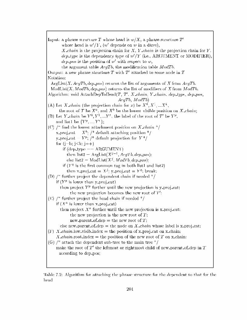
Input: a phrase structure T whose head is w=X, a phrase structure T 0
whose head is w0=Y , (w0 depends on w in a dtree),X chain is the projection chain for X, Y chain is the projection chain for Y ,dep type is the dependency type of w0=Y (i.e., ARGUMENT or MODIFIER),dep pos is the position of w0 with respect to w,the argument table ArgTb, the modi�cation table ModTb.
Output: a new phrase structure T with T 0 attached to some node in TNotation:ArgList(X;ArgTb; dep pos) returns the list of arguments of X from ArgTb.ModList(X;ModTb; dep pos) returns the list of modi�ers of X from ModTb.
Algorithm: void AttachDepToHead(T , T 0, X chain, Y chain, dep type, dep pos,ArgTb, ModTb)
(A) Let X chain (the projection chain for x) be X0;X1; :::Xk,the root of T be Xa, and Xb be the lowest visible position on X chain;
(B) Let Y chain be Y 0; Y 1; :::Y r, the label of the root of T 0 be Y p,and list1 be fY p; :::; Y rg;
(C) /* �nd the lowest attachment position on X chain */x proj cat = Xb; /* default attaching position */y proj cat = Y p; /* default projection for Y */for (j=b; j�k; j++)
if (dep type == ARGUMENT)then list2 = ArgList(Xj�1; ArgTb; dep pos);else list2 = ModList(Xj ;ModTb; dep pos);
if (Y q is the �rst common tag in both list1 and list2)then x proj cat = Xj ; y proj cat = Y q; break;
(D) /* further project the dependent chain if needed */if (Y p is lower than y proj cat)then project Y p further until the new projection is y proj cat;
the new projection becomes the new root of T 0;(E) /* further project the head chain if needed */
if (Xa is lower than x proj cat)then project Xa further until the new projection is x proj cat;
the new projection is the new root of T ;new parent of dep = the new root of T ;
else new parent of dep = the node on X chain whose label is x proj cat;(F) X chain.low visib index = the position of x proj cat on x chain;
X chain.root index = the position of the new root of T on x chain;(G) /* attach the dependent sub-tree to the main tree */
make the root of T 0 the leftmost or rightmost child of new parent of dep in Taccording to dep pos;
Table 7.2: Algorithm for attaching the phrase structure for the dependent to that for thehead
204
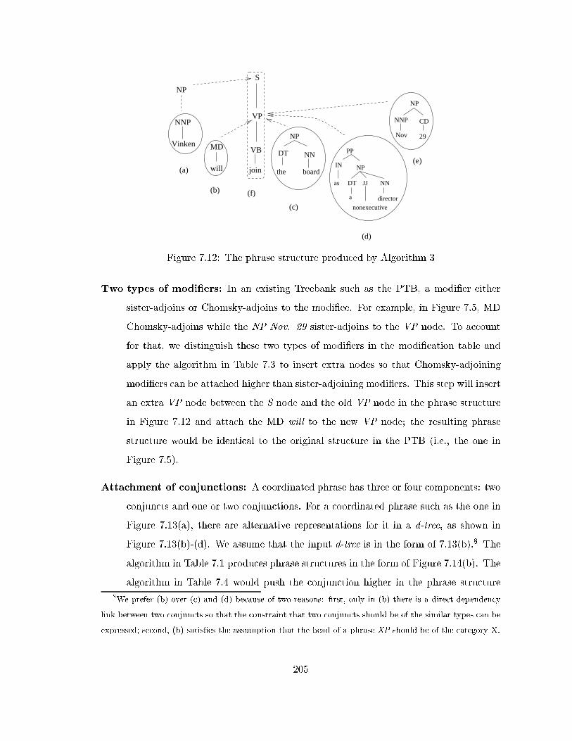
MD
will
VB
join
VP
S
NNP
VinkenNP
DT NN
boardthe
PP
NP
DT JJ NN
a directornonexecutive
IN
as
CD
NP
NNP
Nov 29
NP
(a)
(b)
(c)
(d)
(e)
(f)
Figure 7.12: The phrase structure produced by Algorithm 3
Two types of modi�ers: In an existing Treebank such as the PTB, a modi�er either
sister-adjoins or Chomsky-adjoins to the modi�ee. For example, in Figure 7.5, MD
Chomsky-adjoins while the NP Nov. 29 sister-adjoins to the VP node. To account
for that, we distinguish these two types of modi�ers in the modi�cation table and
apply the algorithm in Table 7.3 to insert extra nodes so that Chomsky-adjoining
modi�ers can be attached higher than sister-adjoining modi�ers. This step will insert
an extra VP node between the S node and the old VP node in the phrase structure
in Figure 7.12 and attach the MD will to the new VP node; the resulting phrase
structure would be identical to the original structure in the PTB (i.e., the one in
Figure 7.5).
Attachment of conjunctions: A coordinated phrase has three or four components: two
conjuncts and one or two conjunctions. For a coordinated phrase such as the one in
Figure 7.13(a), there are alternative representations for it in a d-tree, as shown in
Figure 7.13(b)-(d). We assume that the input d-tree is in the form of 7.13(b).8 The
algorithm in Table 7.1 produces phrase structures in the form of Figure 7.14(b). The
algorithm in Table 7.4 would push the conjunction higher in the phrase structure
8We prefer (b) over (c) and (d) because of two reasons: �rst, only in (b) there is a direct dependency
link between two conjuncts so that the constraint that two conjuncts should be of the similar types can be
expressed; second, (b) satis�es the assumption that the head of a phrase XP should be of the category X.
205
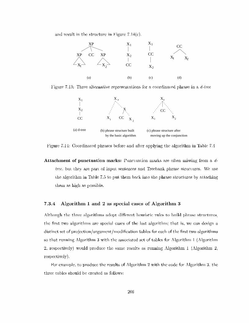
and result in the structure in Figure 7.14(c).
XP CC XP
XP
X X21
X
X
CC
1
2 CC
X
X
1
2
CC
X X1 2
(b) (d)(a) (c)
Figure 7.13: Three alternative representations for a coordinated phrase in a d-tree
X
X
CC
1
2
X
CC
X X1 2
a
X
X
X1 2
a
CC
X
(a) d-tree (c) phrase structure after
moving up the conjunction
(b) phrase structure built
by the basic algorithm
Figure 7.14: Coordinated phrases before and after applying the algorithm in Table 7.4
Attachment of punctuation marks: Punctuation marks are often missing from a d-
tree, but they are part of input sentences and Treebank phrase structures. We use
the algorithm in Table 7.5 to put them back into the phrase structures by attaching
them as high as possible.
7.3.4 Algorithm 1 and 2 as special cases of Algorithm 3
Although the three algorithms adopt di�erent heuristic rules to build phrase structures,
the �rst two algorithms are special cases of the last algorithm; that is, we can design a
distinct set of projection/argument/modi�cation tables for each of the �rst two algorithms
so that running Algorithm 3 with the associated set of tables for Algorithm 1 (Algorithm
2, respectively) would produce the same results as running Algorithm 1 (Algorithm 2,
respectively).
For example, to produce the results of Algorithm 2 with the code for Algorithm 3, the
three tables should be created as follows:
206
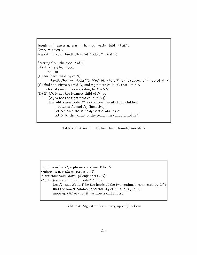
Input: a phrase structure T, the modi�cation table ModTbOutput: a new TAlgorithm: void HandleChomAdjNodes(T , ModTb)
Starting from the root R of T :(A) if (R is a leaf node)
return;(B) for (each child Ni of R)
HandleChomAdjNodes(Ti, ModTb), where Ti is the subtree of T rooted at Ni
(C) �nd the leftmost child Ni and rightmost child Nj that are notchomsky-modi�ers according to ModTb;
(D) if ((Ni is not the leftmost child of N) or(Nj is not the rightmost child of N))then add a new node N� as the new parent of the children
between Ni and Nj (inclusive);let N� have the same syntactic label as N ;let N be the parent of the remaining children and N�;
Table 7.3: Algorithm for handling Chomsky modi�ers
Input: a d-tree D, a phrase structure T for DOutput: a new phrase structure TAlgorithm: void MoveUpConjNode(T , D)(A) for (each conjunction node CC in T )
Let X1 and X2 in T be the heads of the two conjuncts connected by CC;�nd the lowest common ancestor Xa of X1 and X2 in T;move up CC so that it becomes a child of Xa;
Table 7.4: Algorithm for moving up conjunctions
207

Input: a phrase structure T, the input sentence W (w1w2:::wn)Output: a new phrase structure TAlgorithm: void AttachPuncMarkToTtree(T , W )(A) for (each punctuation mark w)
create a leaf node Nl for w;�nd the word wi (wj , resp.) such that wi (wj , resp.) is the closest word to wthat is to the left (right, resp.) of w and is not a punctuation mark;
if (both wi and wj exist)then �nd the leaf nodes Ni and Nj in T for the two words;
�nd the lowest common ancestor Nr of Ni and Nj in T ;make Nl a child of Nr;
else make Nl a child of the root of T ;
Table 7.5: Algorithm for attaching punctuation marks to phrase structures
Input: a sentence W , the d-tree D for W ,the projection table ProjT b, the argument table ArgTb,modi�cation table ModTb
Output: a phrase structure TAlgorithm: ttree ConvDtreeToTtree(W , D, ProjT b, ArgTb, ModTb)(A) T = BuildTtree(D, ProjT b, ArgTb, ModTb);(B) HandleChomAdjNodes(T , ModTb);(C) MoveUpConjNode(T , D);(D) AttachPuncMarkToTtree(T , W );(E) return T ;
Table 7.6: The complete Algorithm 3 for converting d-tree to phrase structure
208
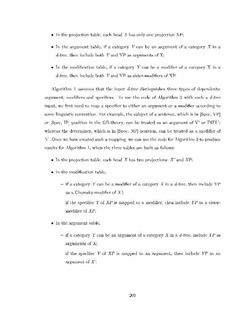
� In the projection table, each head X has only one projection XP;
� In the argument table, if a category Y can be an argument of a category X in a
d-tree, then include both Y and YP as arguments of X;
� In the modi�cation table, if a category Y can be a modi�er of a category X in a
d-tree, then include both Y and YP as sister-modi�ers of XP.
Algorithm 1 assumes that the input d-tree distinguishes three types of dependents:
argument, modi�ers and speci�ers. To use the code of Algorithm 3 with such a d-tree
input, we �rst need to map a speci�er to either an argument or a modi�er according to
some linguistic convention. For example, the subject of a sentence, which is in [Spec, VP]
or [Spec, IP] position in the GB-theory, can be treated as an argument of V' or INFL';
whereas the determiner, which is in [Spec, NP] position, can be treated as a modi�er of
N'. Once we have created such a mapping, we can use the code for Algorithm 3 to produce
results for Algorithm 1, when the three tables are built as follows:
� In the projection table, each head X has two projections: X' and XP;
� In the modi�cation table,
{ if a category Y can be a modi�er of a category X in a d-tree, then include YP
as a Chomsky-modi�er of X';
{ if the speci�er Y of XP is mapped to a modi�er, then include YP as a sister-
modi�er of XP.
� In the argument table,
{ if a category Y can be an argument of a category X in a d-tree, include YP as
arguments of X;
{ if the speci�er Y of XP is mapped to an argument, then include YP as an
argument of X'.
209
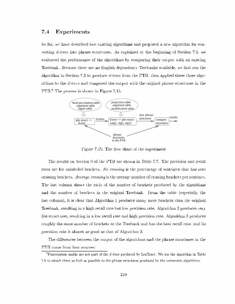
7.4 Experiments
So far, we have described two existing algorithms and proposed a new algorithm for con-
verting d-trees into phrase structures. As explained at the beginning of Section 7.3, we
evaluated the performance of the algorithms by comparing their output with an existing
Treebank. Because there are no English dependency Treebanks available, we �rst ran the
algorithm in Section 7.2 to produce d-trees from the PTB, then applied these three algo-
rithms to the d-trees and compared the output with the original phrase structures in the
PTB.9 The process is shown in Figure 7.15.
tagset tableargument table
head percolation table
modification table
resultsnew phrase
d-treephr-struct => d-tree => phr-struct
(alg1, alg2, alg3)
structures
structures
d-trees comparestructures
in the PTB
phrase
projection tableargument table
Figure 7.15: The ow chart of the experiment
The results on Section 0 of the PTB are shown in Table 7.7. The precision and recall
rates are for unlabeled brackets. No crossing is the percentage of sentences that has zero
crossing brackets. Average crossing is the average number of crossing brackets per sentence.
The last column shows the ratio of the number of brackets produced by the algorithms
and the number of brackets in the original Treebank. From the table (especially the
last column), it is clear that Algorithm 1 produces many more brackets than the original
Treebank, resulting in a high recall rate but low precision rate. Algorithm 2 produces very
at structures, resulting in a low recall rate and high precision rate. Algorithm 3 produces
roughly the same number of brackets as the Treebank and has the best recall rate, and its
precision rate is almost as good as that of Algorithm 2.
The di�erences between the output of the algorithms and the phrase structures in the
PTB come from four sources:
9Punctuation marks are not part of the d-trees produced by LexTract. We use the algorithm in Table
7.5 to attach them as high as possible to the phrase structures produced by the conversion algorithms.
210

recall precision no crossing average test/(%) (%) (%) crossing gold
Alg1 81.34 32.81 50.81 0.90 2.48Alg2 54.24 91.50 94.90 0.10 0.59Alg3 86.24 88.72 84.33 0.27 0.98
Table 7.7: Performance of three conversion algorithms on Section 0 of the PTB
(S1) Annotation errors in the PTB
(S2) Errors in the language-speci�c tables used by the algorithms in Sections 7.2 and 7.3
(e.g., the head percolation table, the projection table, the argument table, and the
modi�cation table)
(S3) The imperfection of the conversion algorithm in Section 7.2 (which converts phrase
structures to d-trees)
(S4) Mismatches between the heuristic rules used by the algorithms in Section 7.3 and
the annotation schemata adopted by the PTB
To estimate the contribution of (S1){(S4) to the di�erences between the output of
Algorithm 3 and the phrase structures in the PTB, we manually examined the �rst twenty
sentences in Section 0. Out of thirty-one di�erences in bracketing, seven are due to (S1),
three are due to (S2), seven are due to (S3), and the remaining fourteen mismatches are
due to (S4).
While correcting annotation errors to eliminate (S1) requires much human e�ort, it
is quite straightforward to correct the errors in the language-speci�c tables and therefore
eliminate the mismatches caused by (S2). For (S3), we mentioned in Section 7.2 that the
algorithm chose the wrong heads for the noun phrases with the appositive construction.
As for (S4), we found several exceptions (as shown in Table 7.8) to the one-projection-
chain-per-category assumption (i.e., the assumption that there is a unique projection chain
for each POS tag), an assumption which was used by all three algorithms in Section 7.3.
The performance of the conversion algorithms in Section 7.2 and 7.3 could be improved
by using additional heuristic rules or statistical information. For instance, Algorithm 3 in
Section 7.3 could use a heuristic rule that says that an adjective (JJ) projects to an NP if
211

the JJ follows the determiner the and the JJ is not followed by a noun as in the rich are
getting richer, and it projects to an ADJP in other cases. Notice that such heuristic rules
are Treebank-dependent.
most likely projection other projection(s)
JJ ! ADJP JJ ! NPCD ! NP CD ! QP ! NPVBN ! VP ! S VBN ! VP ! RRCNN ! NP NN ! NX ! NPVBG ! VP ! S VBG ! PP
Table 7.8: Some examples of heads with more than one projection chain
7.5 Discussion
In this section, we argue for including empty categories in dependency structures. We also
give an algorithm that builds grammars and derivation trees from dependency structures
directly.
7.5.1 Extending Algorithm 3
We can extend Algorithm 3 in two ways. First, in the current algorithm, we assume that
the argument/adjunct distinction is marked explicitly in the input dependency structure.
We can relax this constraint: instead of requiring the type of a dependency link to be AR-
GUMENT or ADJUNCT, the dependency type can be things such as agent and theme,
or no label at all. We treat these dependency types the same way as we treat the function
tags in a phrase-structure. Now to build a phrase structure from a dependency structure,
the only thing that we need to change in Algorithm 3 is line (C) in Table 7.2. Another
extension to Algorithm 3 is to relax the constraint that each category has only one pro-
jection chains for a category. Once the multiple projection chains are We then need to use
either heuristic rules or statistical information to
212
7.5.2 Empty categories in dependency structures
Empty categories are often explicitly marked in phrase-structures, but they are not always
included in dependency structures. We believe that including empty categories in depen-
dency structures has many bene�ts. First, empty categories are useful for NLP applications
such as machine translation. To translate a sentence from one language to another, many
machine translation systems �rst create the dependency structure for the sentence in the
source language, then produce the dependency structure for the target language, and �-
nally generate a sentence in the target language. If the source language (e.g., Chinese and
Korean) allows argument deletion and the target language (e.g., English) does not, it is
crucial that the dropped argument (which is a type of empty category) is explicitly marked
in the source dependency structure, so that the machine translation systems are aware of
the existence of the dropped argument and can handle the situation accordingly. The sec-
ond bene�t of including empty categories in dependency structures is that it can improve
the performance of the conversion algorithms in Section 7.3, because the phrase structures
produced by the algorithms would then have empty categories as well, just like the phrase
structures in the PTB. Third, if a sentence includes a non-projective construction such as
wh-movement in English, and if the dependency tree did not include an empty category to
show the movement, traversing the dependency tree would yield the wrong word order.10
7.5.3 Running LexTract on a dependency Treebank
In Chapter 5, we give algorithms that takes phrase-structure Treebanks as input, and
produce grammars (LTAGs and CFGs) and derivation trees as output. In Section 7.3,
we have proposed an algorithm for converting dependency structures to phrase structures.
Therefore, given a dependency Treebank, we can simply convert the dependency Treebank
to a phrase-structure Treebank using that conversion algorithm, then run algorithms in
Chapter 5 to produce Treebank grammars and derivation trees.
We can also produce grammars and derivation trees from the dependency structures
directly without �rst creating the corresponding phrase structures. The algorithm (shown
10For more discussion of non-projective constructions, see (Rambow and Joshi, 1997).
213

in Table 7.9 and 7.10) is very similar to the Algorithm 3 in Section 7.3 (see Table 7.1
and 7.2). The main di�erence is that the algorithm in Table 7.9 and 7.10 produces an
elementary tree for each word in the d-tree, whereas the algorithm in Section 7.3 produces
one phrase structure for the whole d-tree.
Figure 7.16 shows a d-tree, which is the same as the one in Figure 7.6 except that
it includes the POS tags for the words and marks dependents as either arguments (with
solid lines) or adjuncts (with dashed lines). Similar notation is used in Figures 7.18 and
7.19 later on. Given this d-tree, the algorithm will produce the elementary trees in Figure
7.17. Another way to understand the algorithm is: the algorithm decomposes the d-tree in
Figure 7.16 into a list of dependent units as in Figure 7.18, and each unit corresponds to an
elementary tree in Figure 7.17. By decompose, we mean that we can de�ne two operations
as shown in Figure 7.19. The �rst operation is similar to the substitution operation in the
LTAG formalism, where the lexical head wi of an argument is added to the dependency
tree. The second one is similar to the adjoining operation, where the lexical head wj of an
adjunct is added to the dependency tree.11 Combining the units in Figure 7.18 via these
two operations will produce the d-tree in Figure 7.16.
Vinken/NNP will/MD board/NN
the/DT
as/IN
nonexecutive/JJa/DT
director/NN Nov/NNP
29/CD
join/VB
Figure 7.16: A dependency tree that marks the argument/adjunct distinction
Once we have built an elementary tree for each word in the d-tree, adding those ele-
mentary trees to the nodes in the d-tree will result in the derivation tree for the sentence.
11In the second operation, the position of the adjunct with respect to the arguments of the head is not
speci�ed in the resulting d-tree. For example, a right modi�er can appear before the �rst right argument,
after the last right argument, or any position in between.
214

Input: a d-tree D, the projection table ProjT b, the argument table ArgTb,the modi�cation table ModTb
Output: a list of elementary trees ESetNotation: Ei is the current elementary tree for the word wi;
Di is the sub-dtree of D whose root is wi
ESeti is the set of elementary trees for the sub-dtree Di;Yi is the POS tag of the word wi;
Algorithm: etrees BuildEtrees(D, ProjT b, ArgTb, ModTb)
Starting from the root RD of D, let the node be w/X andit has k dependents wi/Yi (1 � i � k).
(A) build a node w/X, let E be a singleton elementary tree that includes onlythe node w/x as its anchor;
(B) if (RD is a leaf node)then ESet = f E g;
return ESet;(C) Let X chain (X0; :::;Xk) be the projection chain for head X according to ProjT b;(D) Let X chain.root index be 1;
Project X to X1 and let X1 be the root of E
/* (E) { (F) handle left dependents */(E) Let X chain.low visib index be 1;(F) for (i = kl; i >= 1; i��) /* kl is the number of X's left dependents */
Let the current left dependent be wi/Yi; dep type is its dependency type;Let Y chain be the projection chain for Yi according to ProjT b;build a set of elementary tree ESeti for the sub-dtree Di rooted at wi/Yi;let Ei be the current elementary tree anchored by wi;UpdateEtrees(E, Ei, X chain, Y chain, dep type, LEFT, ArgTb, ModTb);ESet = ESet [ ESeti;
/* (G)-(H) attach right dependents */(G) Let X chain.low visib index be 1;(H) for (i = kl + 1; i <= k; i++)
Let the current right dependent be wi/Yi; dep type is its dependency type;Let Y chain be the projection chain for yi according to ProjT b;build a set of elementary tree ESeti for the sub-dtree Di rooted at wi/Yi;let Ei be the current elementary tree anchored by wi;UpdateEtrees(E, Ei, X chain, Y chain, dep type, LEFT, ArgTb, ModTb);ESet = ESet [ ESeti;
(I) ESet = ESet [ fEg; return ESet;
Table 7.9: Algorithm for building elementary trees directly from a d-tree
215
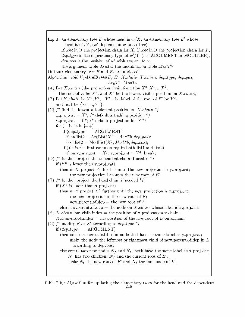
Input: an elementary tree E whose head is w=X, an elementary tree E0 whosehead is w0=Y , (w0 depends on w in a dtree),
X chain is the projection chain for X, Y chain is the projection chain for Y ,dep type is the dependency type of w0=Y (i.e. ARGUMENT or MODIFIER),dep pos is the position of w0 with respect to w,the argument table ArgTb, the modi�cation table ModTb
Output: elementary tree E and Ei are updatedAlgorithm: void UpdateEtrees(E, E0, X chain, Y chain, dep type, dep pos,
ArgTb, ModTb)(A) Let X chain (the projection chain for x) be X0;X1; :::Xk ,
the root of E be Xa, and Xb be the lowest visible position on X chain;(B) Let Y chain be Y 0; Y 1; :::Y r, the label of the root of E0 be Y p,
and list1 be fY p; :::; Y rg;(C) /* �nd the lowest attachment position on X chain */
x proj cat = Xb; /* default attaching position */y proj cat = Y p; /* default projection for Y */for (j=b; j�k; j++)
if (dep type == ARGUMENT)then list2 = ArgList(Xj�1; ArgTb; dep pos);else list2 = ModList(Xj ;ModTb; dep pos);
if (Y q is the �rst common tag in both list1 and list2)then x proj cat = Xj ; y proj cat = Y q; break;
(D) /* further project the dependent chain if needed */if (Y p is lower than y proj cat)then in E0 project Y p further until the new projection is y proj cat;
the new projection becomes the new root of E0.(E) /* further project the head chain if needed */
if (Xa is lower than x proj cat)then in E project Xa further until the new projection is x proj cat;
the new projection is the new root of E;new parent of dep = the new root of E;
else new parent of dep = the node on X chain whose label is x proj cat;(F) X chain.low visib index = the position of x proj cat on x chain;
X chain.root index = the position of the new root of E on x chain;(G) /* modify E or E0 according to dep type */
if (dep type == ARGUMENT)then create a new substitution node that has the same label as y proj cat;
make the node the leftmost or rightmost child of new parent of dep in Eaccording to dep pos;
else create two new nodes Nf and Nr, both have the same label as x proj cat;Nr has two children: Nf and the current root of E0;make Nr the new root of E0 and Nf the foot node of E0.
Table 7.10: Algorithm for updating the elementary trees for the head and the dependent216

NP
Vinken
NNP
S
NP
VB
join
NP
VPDT NP*
NP
the
NP
board
NN
(a) (b) (c) (d) (e)
VP
VP* PP
NPP
as
DT NP*
NP
a
NP
NP*JJ
nonexecutive
NP
NN
director
NP
CD
29
NP*NNP
Nov
NP
(f) (g) (h) (i) (k)(j)
VP
MD VP*
will
Figure 7.17: The elementary trees built directly from the dependency tree in Figure 7.16
-/VB
will/MD
join/VB
_/NNP _/NN
_/NN
the/DT
_/VB
as/IN
_/NN
_/NN
a/DT
_/NN
nonexecutive/JJ
CD
Nov/NNP
Vinken/NNP board/NN
NN/director 29/CD
(g)
(b)(a) (c) (d) (e)
(f) (h) (i) (j) (k)
Figure 7.18: The dependency units that form the dependency tree in Figure 7.16
7.6 Summary
In this chapter, we have proposed a new algorithm that converts dependency structures
to phrase structures and compared it with two existing ones. We have shown that our
algorithm subsumes the two existing ones. By using simple heuristic rules and taking as
input certain kinds of language-speci�c information such as the types of arguments and
modi�ers that a head can take, our algorithm produces phrase structures that are very
close to the ones in an existing phrase-structure Treebank; moreover, the quality of the
phrase structures produced by our algorithm can be further improved when more language-
speci�c information is used. We also give an algorithm that converts phrase structures to
dependency structures.
217
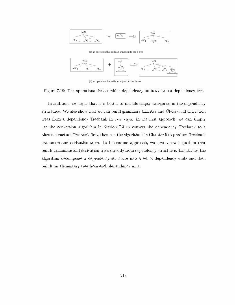
_/Yn
w/X
i-/Y 1 _/Y ... ...
... ... _/Yn
w/X
i-/Y 1
... ...
... ...w /Y i
_/Yn
w/X
i-/Y 1 _/Y ... ...
... ...w /Zj j w /Zj j_/Yn
w /Y ii
w/X
...
_/X
-/Y 1 ... _/Y i ...
...
(a) an operation that adds an argument to the d-tree
(b) an operation that adds an adjunct to the d-tree
Figure 7.19: The operations that combine dependency units to form a dependency tree
In addition, we argue that it is better to include empty categories in the dependency
structures. We also show that we can build grammars (LTAGs and CFGs) and derivation
trees from a dependency Treebank in two ways: in the �rst approach, we can simply
use the conversion algorithm in Section 7.3 to convert the dependency Treebank to a
phrase-structure Treebank �rst, then run the algorithms in Chapter 5 to produce Treebank
grammars and derivation trees. In the second approach, we give a new algorithm that
builds grammars and derivation trees directly from dependency structures. Intuitively, the
algorithm decomposes a dependency structure into a set of dependency units and then
builds an elementary tree from each dependency unit.
218

Chapter 8
Conclusion
Grammars are valuable resources for natural language processing. In this dissertation,
we pointed out the problems with the traditional approach to grammar development and
provided two systems that build grammars automatically from either descriptions or Tree-
banks. In this chapter, we summarize the contributions of this work and point out direc-
tions for further study.
8.1 Contributions
Traditionally, grammars are built by hand. In Chapter 1, we listed six problems with
this approach. To address these problems, we �rst de�ned the prototypes of the target
grammars, then built two systems, LexOrg and LexTract, that generate grammars auto-
matically from either descriptions or Treebanks. The di�erences between the traditional
approach, LexOrg, and LexTract are summarized in Table 1.1, repeated as Table 8.1. We
use symbols �, 2, and p to indicate that an approach did not solve the problem, partially
solved the problem, and solved the problem, respectively. From the table, it is clear that
LexOrg and LexTract have advantages over the traditional approach.
8.1.1 The prototypes of elementary trees
Before building a grammar for a particular language, we identi�ed four types of information
that should be included in elementary trees of a grammar. They are the head and its
219
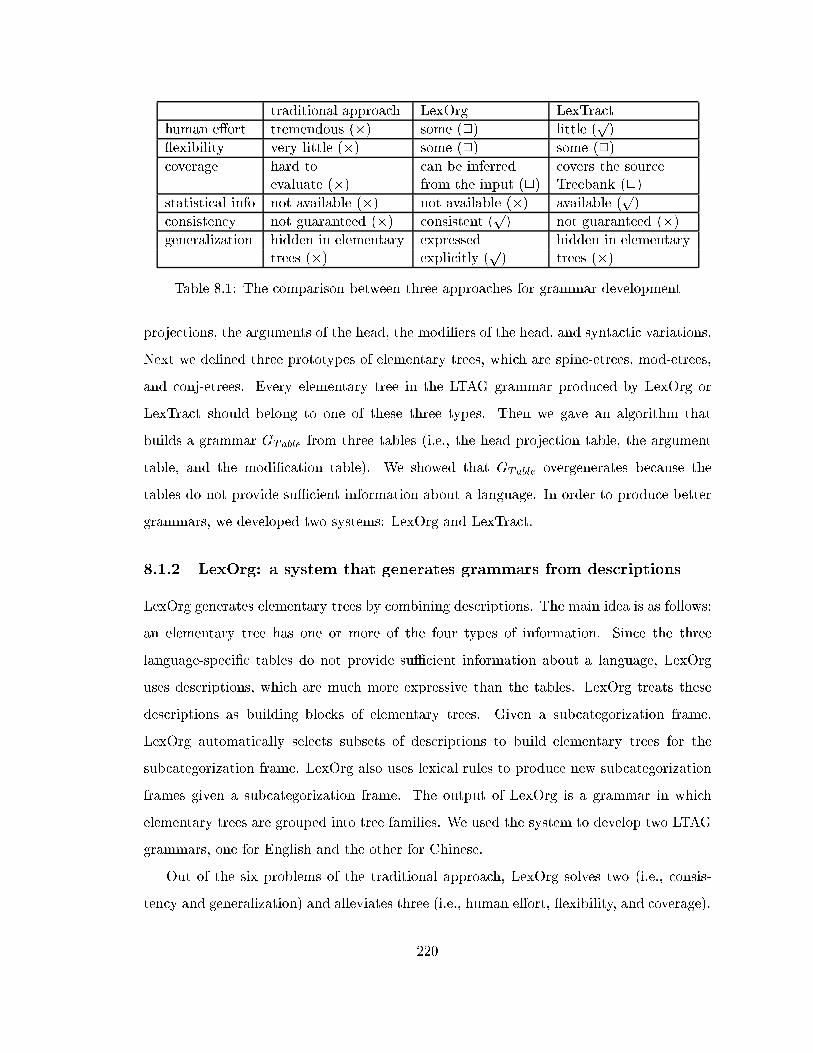
traditional approach LexOrg LexTract
human e�ort tremendous (�) some (2) little (p)
exibility very little (�) some (2) some (2)
coverage hard to can be inferred covers the sourceevaluate (�) from the input (2) Treebank (2)
statistical info not available (�) not available (�) available (p)
consistency not guaranteed (�) consistent (p) not guaranteed (�)
generalization hidden in elementary expressed hidden in elementarytrees (�) explicitly (
p) trees (�)
Table 8.1: The comparison between three approaches for grammar development
projections, the arguments of the head, the modi�ers of the head, and syntactic variations.
Next we de�ned three prototypes of elementary trees, which are spine-etrees, mod-etrees,
and conj-etrees. Every elementary tree in the LTAG grammar produced by LexOrg or
LexTract should belong to one of these three types. Then we gave an algorithm that
builds a grammar GTable from three tables (i.e., the head projection table, the argument
table, and the modi�cation table). We showed that GTable overgenerates because the
tables do not provide suÆcient information about a language. In order to produce better
grammars, we developed two systems: LexOrg and LexTract.
8.1.2 LexOrg: a system that generates grammars from descriptions
LexOrg generates elementary trees by combining descriptions. The main idea is as follows:
an elementary tree has one or more of the four types of information. Since the three
language-speci�c tables do not provide suÆcient information about a language, LexOrg
uses descriptions, which are much more expressive than the tables. LexOrg treats these
descriptions as building blocks of elementary trees. Given a subcategorization frame,
LexOrg automatically selects subsets of descriptions to build elementary trees for the
subcategorization frame. LexOrg also uses lexical rules to produce new subcategorization
frames given a subcategorization frame. The output of LexOrg is a grammar in which
elementary trees are grouped into tree families. We used the system to develop two LTAG
grammars, one for English and the other for Chinese.
Out of the six problems of the traditional approach, LexOrg solves two (i.e., consis-
tency and generalization) and alleviates three (i.e., human e�ort, exibility, and coverage).
220
First, the tree structures that are shared by many templates are represented as descrip-
tions. Users of LexOrg build and maintain descriptions, rather than templates. If they
want to change the analysis of a certain phenomenon (e.g., wh-movement), they need to
modify only the description that represents the phenomenon. LexOrg will propagate the
modi�cation in the description to all the templates that subsume the description. As a
result, LexOrg greatly improves the consistency of a grammar, reduces human e�ort, and
makes it easier to modify a grammar. It is also easy to infer from the input of LexOrg
(i.e., subcategorization frames, lexical rules, and descriptions) what syntactic phenomena
are covered by the resulting grammar. Second, the underlying linguistic information (such
as wh-movement) is expressed explicitly as descriptions and so forth, so it is easy to grasp
the main characteristics of a language and to compare languages. Compared with three
other systems (namely, HyTAG, the DATR system, and Candito's system), LexOrg is more
elegant in that it does not need hand-crafted lexical hierarchies (or inheritance networks),
it does not require users to provide constraints on how descriptions should be combined,
and it needs only one description to specify the information for a syntactic variation such
as wh-movement.
8.1.3 LexTract: a system that extracts grammars from Treebanks
Conceptually, LexTract uses a Treebank as a �lter to throw away the elementary trees in
GTable that are not used to handle the sentences in a Treebank. In practice, it extracts
grammars in two steps. In the �rst step, it determines the types (i.e., head, argument, or
adjunct) of each node in a ttree, and then creates a derived tree in which the three types
of nodes are treated di�erently. In the second step, it decomposes the derived tree into a
set of etrees.
Out of six problems of the traditional approach, LexOrg solves two (i.e., human e�ort
and statistical information) and alleviates two (i.e., exibility and coverage). First, given a
Treebank, it takes very little human e�ort to build three language-speci�c tables. Once the
tables are ready, running LexTract on the Treebank will produce a grammar in little time.
Second, LexTract produces not only a Treebank grammar, but also the information about
how frequently certain elementary structures are combined to form syntactic structures;
221
to be more speci�c, the system produces a unique derivation tree for each sentence in the
Treebank. This frequency information can be used to train a statistical LTAG parser.
Third, LexTract allows its users to have some control over the type of Treebank grammar
to be extracted. The users can run LexTract with di�erent settings of the tables and
other parameters to get several di�erent Treebank grammars, and then choose the one
that best �ts their goals. Fourth, the grammar produced by LexTract is guaranteed to
cover the source Treebank. If the Treebank is a good representative of the language itself,
the Treebank grammar will have very good coverage of the language.
In addition to providing Treebank grammars, LexTract is also used in several tasks:
� A Treebank grammar can be used as a stand-alone grammar. In addition, matching
templates in a Treebank grammar with the templates in a hand-crafted grammar
allows us to estimate the coverage of the hand-crafted grammar and �nd the con-
structions that are not covered by that grammar. Our experiments show that the
XTAG grammar covers 97.2% of the template tokens in the English Penn Treebank
(Xia and Palmer, 2000).
� We have compared the Treebank grammars for three languages (English, Chinese,
and Korean) and shown that the majority of the core grammar structures for these
three languages are easily inter-mappable (Xia et al., 2001).
� The Treebank grammar and derivation trees produced by LexTract are used to train
a Supertagger (Xia et al., 2000a) and a statistical LTAG parser (Sarkar, 2001) with
satisfactory results.
� We have used the Treebank grammar to detect certain types of annotation errors in
the Chinese Penn Treebank.
� We have used LexTract to �nd all the examples in the English Penn Treebank that
seem to violate the Tree-locality Hypothesis and classi�ed them according to the
underlying constructions (Xia and Bleam, 2000).
All these applications indicate that LexTract is not only an engineering tool of great
value, but it is also useful for investigating theoretical linguistics.
222
For people who want to use LexOrg or LexTract to build a grammar, they should
choose one system or the other based on the availability of Treebanks, the applications for
which the target grammar is used, and other considerations. If a Treebank is available,
LexTract is often more desirable because it requires little human e�ort, it allows its users to
change the language-speci�c tables or other parameters to get di�erent grammars from the
same Treebank, and it provides statistical information that can be used to train statistical
parsers or Supertaggers. If a Treebank is not available, there are two options: one is to
create descriptions, subcategorization frames, and lexical rules and then use LexOrg to
generate a grammar; the other is to create a Treebank and then use LexTract to extract a
grammar from it. Creating a Treebank requires more human e�orts than creating the input
to LexOrg. Nevertheless, once a Treebank is available, all kinds of NLP tools including
LexTract can bene�t from it.
8.1.4 The role of linguistic experts in grammar development
LexOrg and LexTract greatly reduce human e�ort in grammar development, but they
cannot replace the role of linguistic experts. In LexOrg, the users have to provide LexOrg
with descriptions, subcategorization frames, and lexical rules. Creating such input requires
linguistic knowledge. Building language-speci�c tables for LexTract does not require much
linguistic expertise but LexTract needs a Treebank which is often designed by scholars with
a solid linguistic background. In Appendix B, we discuss in detail the approach that we
used for building the Chinese Penn Treebank, including the development of the guidelines
for segmentation, POS tagging and syntactic bracketing, our methodology for quality
control, and the roles of various NLP tools. From this experience, we conclude that the
process of writing annotation guidelines for a Treebank | which is one of the major tasks
in Treebank development | is very similar to the process of manually crafting a grammar
in that both processes require a thorough study of the linguistics literature, extensive
discussion with linguists, and possible revisions to account for new data. Therefore, it is
not surprising that a grammar extracted from a high-quality Treebank by LexTract may
look very much like a hand-crafted grammar. We believe that the participation of linguistic
experts is crucial for the success of any grammar or Treebank development project.
223
8.1.5 Relationship between two types of syntactic representation
Two of the most commonly used syntactic representations are phrase structures and de-
pendency structures. In Chapter 7, we addressed the relationship between dependency
structures and phrase structures from a practical perspective; namely, we explored dif-
ferent algorithms that convert between dependency structures and phrase structures. We
proposed an algorithm that converts dependency structures into phrase structures. By us-
ing simple heuristic rules and taking three language-speci�c tables as input, our algorithm
produces phrase structures that are very close to the ones in a phrase-structure Treebank;
moreover, the quality of the phrase structures produced by our algorithm can be further
improved when more language-speci�c information is used. We also argue that including
empty categories in the dependency structures would make the conversion much easier. In
addition, we give an algorithm that converts phrase structures to dependency structures.
This experiment showed that the conversion between phrase structures and dependency
structures is pretty easy as long as suÆcient information (such as empty categories) is
included in the structures.
Furthermore, we proposed two ways to build grammars (LTAGs and CFGs) and deriva-
tion trees from a dependency Treebank: in the �rst approach, we can simply convert the
dependency Treebank to a phrase-structure Treebank using the conversion algorithm in
Section 7.3, and then run the algorithms in Section 5.4 to produce Treebank grammars
and derivation trees. In the second approach, we gave a new algorithm that builds gram-
mars and derivation trees directly from dependency structures. Intuitively, the algorithm
decomposes a dependency structure into a set of dependency units and then builds an
elementary tree from each dependency unit.
8.2 Future work
In this section, we point out directions for future work.
224

8.2.1 Combining the strengths of LexOrg and LexTract
From Table 8.1, it is clear that both LexOrg and LexTract have advantages over the
traditional approach. Grammars generated by LexOrg are consistent and linguistic gener-
alizations are expressed explicitly, whereas running LexTract on a Treebank requires little
human e�ort and the resulting grammar has statistical information. A natural question is
as follows: how can we combine the strengths of both systems?
modification table
argument tableother info
TGhead percolation table
G*T
subcat frames
lexical rules
descriptionsLexOrg
module
newLexTract
Treebank
Figure 8.1: One way to combine LexOrg and LexTract
One possible scenario is shown in Figure 8.1. In this scenario, LexTract extracts from a
Treebank T a grammar GT and other information (such as derivation trees and frequencies
of elementary trees in GT ). GT may include implausible elementary trees that are caused
by annotation errors in the Treebank T . It may also exclude plausible trees which do
not appear in the Treebank. To get a better grammar, we need a new module that takes
the output of LexTract as input and produces subcategorization frames, lexical rules, and
descriptions as output. In Sections 4.9.2 and 5.7, we show that it is possible to decompose
templates to get descriptions and subcategorization frames, but such decompositions are
not always unique. Ideally, the new module should be able to take advantage of frequency
information produced by LexTract to choose the most plausible decompositions. The
output of the new module is then fed to LexOrg to generate a new grammar G�T . If the
new module works properly, the new grammar G�T should be able to exclude implausible
elementary trees in GT that are caused by random annotation errors in the Treebank T ,
and to include plausible elementary trees that are missing from GT as long as other related
elementary trees appear in the Treebank.
To see how G�T can actually include elementary trees that are not in GT , let us assume
a Treebank T has only two sentences: one is who bought that car? the other one is
225

Mary gave John a book. GT built by LexTract has only two elementary trees that are
anchored by verbs, as shown in Figure 8.2(a). Decomposing the templates in GT would
yield the descriptions and subcategorization frames in Figure 8.2(b). When they are fed
to LexOrg, LexOrg builds a new grammar G�T , which has seven elementary trees for verbs,
as shown in Figure 8.2(c). Two of them (i.e., #2 and #4) are in GT , but the other �ve
are new. As a result, G�T can handle not only wh-questions anchored by transitive verbs
and declarative sentences anchored by ditransitive verbs, but also declarative sentences
anchored by transitive verbs and wh-questions anchored by ditransitive verbs.
In summary, the approach shown in Table 8.1 inherits the strengths of both LexOrg
and LexTract: the input to this new system requires little human e�ort, and the users can
change the input tables to get di�erent grammars; the output of the system is a consistent
grammar and linguistic generalizations are expressed explicitly; the output grammar G�T
also has a better coverage than the Treebank grammar GT , as illustrated in Figure 8.2. To
implement this approach, two details need to be worked out. First, how does the module
produce descriptions, subcategorization frames, and lexical rules, given the grammar GT
and frequency information produced by LexTract? Second, how do we assign probabilities
to the elementary trees in G�T , given the frequency information assigned to the trees in
GT ? We leave these for future work.
8.2.2 Building and using parallel Treebanks
Treebanks are a prerequisite for running LexTract and training NLP tools such as POS
taggers and parsers. In Appendix B, we discuss three topics in creating a monolingual
Treebank { making annotation guidelines, ensuring annotation accuracy, and using NLP
tools. Building a parallel Treebank will face a series of new challenges.
The �rst issue is the choice of the corpus for the Treebank. Unlike monolingual texts,
it is not trivial to �nd high-quality bilingual texts that are freely available to the public.
An alternative is to �nd a monolingual corpus and then have it translated into the other
language. A question about the translation is: should we choose the most natural trans-
lation or the one that is as literal as possible so that presumably it is easier for a machine
translation system to learn useful patterns from the parallel Treebank?
226
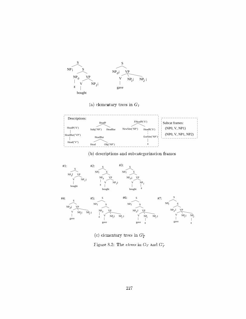
VPNP
V
S
NP NP
gave
1 2
0
S
bought
0
1
VPNP
V NP
NP
S
S
bought
0
1
VPNP
V NPε
VPNP
V
S
NP NP
gave
1 2
0
S
NP
ε
HeadP(’S’)
HeadBar(’VP’)
Head(’V")
Subj(’NP’) HeadBar
HeadP
Obj(’NP’)
HeadBar
Head
NewSite(’NP’)
FHeadP(’S’)
HeadP(’S’)
ExtSite(’NP’)
ε
NP
S
S
bought
0
1
VPNP
V
S
NP NP
gave
1 2
0VPNP
V NPε
NP
S
S
bought
0
1
VPNP
V NP
ε
VPNP
V
S
NP NP
gave
1 2
0
S
NP
ε
VPNP
V
S
NP NP
gave
1 2
0
S
NP
ε
#1: #2: #3:
#4: #5: #6: #7:
Subcat frames:
(NP0, V, NP1)
(NP0, V, NP1, NP2)
Descriptions:
(a) elementary trees in GT
(b) descriptions and subcategorization frames
(c) elementary trees in G�T
Figure 8.2: The etrees in GT and G�T
227

Another issue is the development of NLP tools for parallel Treebank annotation. For
example, given a bilingual text (A, B), if one side (say A) is already bracketed, is there
any way to speed up the annotation of the other side (i.e., B) using the information from
A? A possible approach is to �rst convert the phrase structure PA of language A into its
dependency structure DA (see Section 7.2), then map DA into the dependency structure
DB for language B, next convert DB into the phrase structure PB (see Section 7.3). A
diÆculty of this approach is the well-known structural divergence problem (Dorr, 1993);
that is, a sentence and its translation in other languages may have di�erent syntactic
structures. In another scenario, if A is bracketed and B is not, but there is a parser for
language B, which is trained and tested on a di�erent Treebank, could the information
from A help to improve the parser's performance on B?
Once a parallel Treebank becomes available, we plan to run LexTract on parallel Tree-
banks. For example, running an alignment algorithm on the Treebank would produce
word-to-word mappings. Given such word-to-word mappings and our template matching
algorithm in Section 6.3, we can automatically create lexicalized etree-to-etree mappings,
which can be used for semi-automatic transfer lexicon construction. Furthermore, Lex-
Tract can build derivation trees for each sentence in the corpora. By comparing derivation
trees for parallel sentences in two languages, instances of structural divergence can be
automatically detected.
228
Appendix A
Language-speci�c tables
In this dissertation, we have used �ve language-speci�c tables (namely, the head percolation
table, argument table, tagset table, modi�cation table, and head projection table) to
perform the following tasks:
� We use the head projection table, argument table, and modi�cation table to build the
grammar GTable (see Section 3.3), to �lter out linguistically implausible templates
(See Section 6.1.3), and to convert a dependency structure into a phrase structure
(See Section 7.3.3).
� We use the head percolation table, argument table, and tagset table to build elemen-
tary trees (See Section 5.4).
In this appendix, we �rst explain the formats of the tables, then show the tables that
we built for the English, Chinese and Korean Penn Treebanks.
A.1 The formats of the language-speci�c tables
We brie y mentioned the formats of the language-speci�c tables in Sections 3.3 and 5.3.
In this section, we describe the tables in detail.
229

A.1.1 Tagset table
Each tag in a Treebank tagset must have an entry in the tagset table. An entry has three
�elds. The �rst �eld uses a number to mark the type of the tag; namely, 0 for POS tag, 1
for syntactic tag, 2 for empty category, and 3 for function tag. The second �eld is the name
of the tag (e.g., JJ for an adjective). The third �eld is a possibly empty set of attributes
for the tag, as explained below:
� CONJ: a tag for conjunctions
� UCP: a tag for unlikely coordinated phrase
� PU: a tag for punctuation marks
� PRN: a tag for parenthetical
� ELLIPSIS: a tag for ellipsis
� IGNORE: the word with that tag will be ignored when LexTract builds etrees.
� BUILDMC: an empty category tag that marks \movement". LexTract will build
multi-component sets for the word with that tag and its antecedent (see Sections 5.6
and 6.7).
� HEAD: a tag that always marks heads
� ADJUNCT: a tag that always marks adjuncts
� ARGUMENT: a tag that always marks arguments
A user can use the last three attributes (HEAD, ADJUNCT, ARGUMENT) to inform
LexTract how a function tag should be interpreted when LexTract determines the types
(heads, arguments, and adjuncts) of nodes.
A.1.2 Head percolation table
LexTract uses the head percolation table and the tagset table to choose the head-child of
a category. Each entry in the head percolation table is of the form (x direct y1=y2=:::=yn),
230
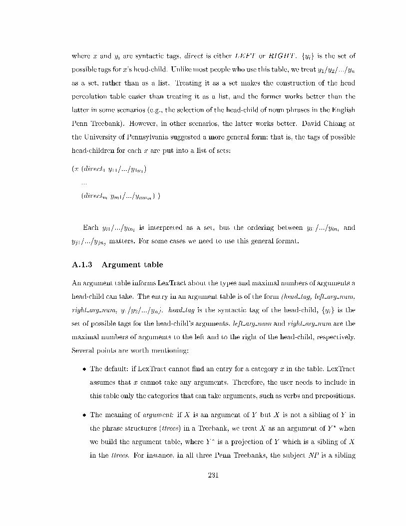
where x and yi are syntactic tags, direct is either LEFT or RIGHT . fyig is the set of
possible tags for x's head-child. Unlike most people who use this table, we treat y1=y2=:::=yn
as a set, rather than as a list. Treating it as a set makes the construction of the head
percolation table easier than treating it as a list, and the former works better than the
latter in some scenarios (e.g., the selection of the head-child of noun phrases in the English
Penn Treebank). However, in other scenarios, the latter works better. David Chiang at
the University of Pennsylvania suggested a more general form; that is, the tags of possible
head-children for each x are put into a list of sets:
(x (direct1 y11=:::=y1n1)
...
(directm ym1=:::=ymnm) )
Each yi1=:::=yini is interpreted as a set, but the ordering between yi1=:::=yini and
yj1=:::=yjnj matters. For some cases we need to use this general format.
A.1.3 Argument table
An argument table informs LexTract about the types and maximal numbers of arguments a
head-child can take. The entry in an argument table is of the form (head tag, left arg num,
right arg num, y1=y2=:::=yn). head tag is the syntactic tag of the head-child, fyig is the
set of possible tags for the head-child's arguments, left arg num and right arg num are the
maximal numbers of arguments to the left and to the right of the head-child, respectively.
Several points are worth mentioning:
� The default: if LexTract cannot �nd an entry for a category x in the table, LexTract
assumes that x cannot take any arguments. Therefore, the user needs to include in
this table only the categories that can take arguments, such as verbs and prepositions.
� The meaning of argument: if X is an argument of Y but X is not a sibling of Y in
the phrase structures (ttrees) in a Treebank, we treat X as an argument of Y � when
we build the argument table, where Y � is a projection of Y which is a sibling of X
in the ttrees. For instance, in all three Penn Treebanks, the subject NP is a sibling
231
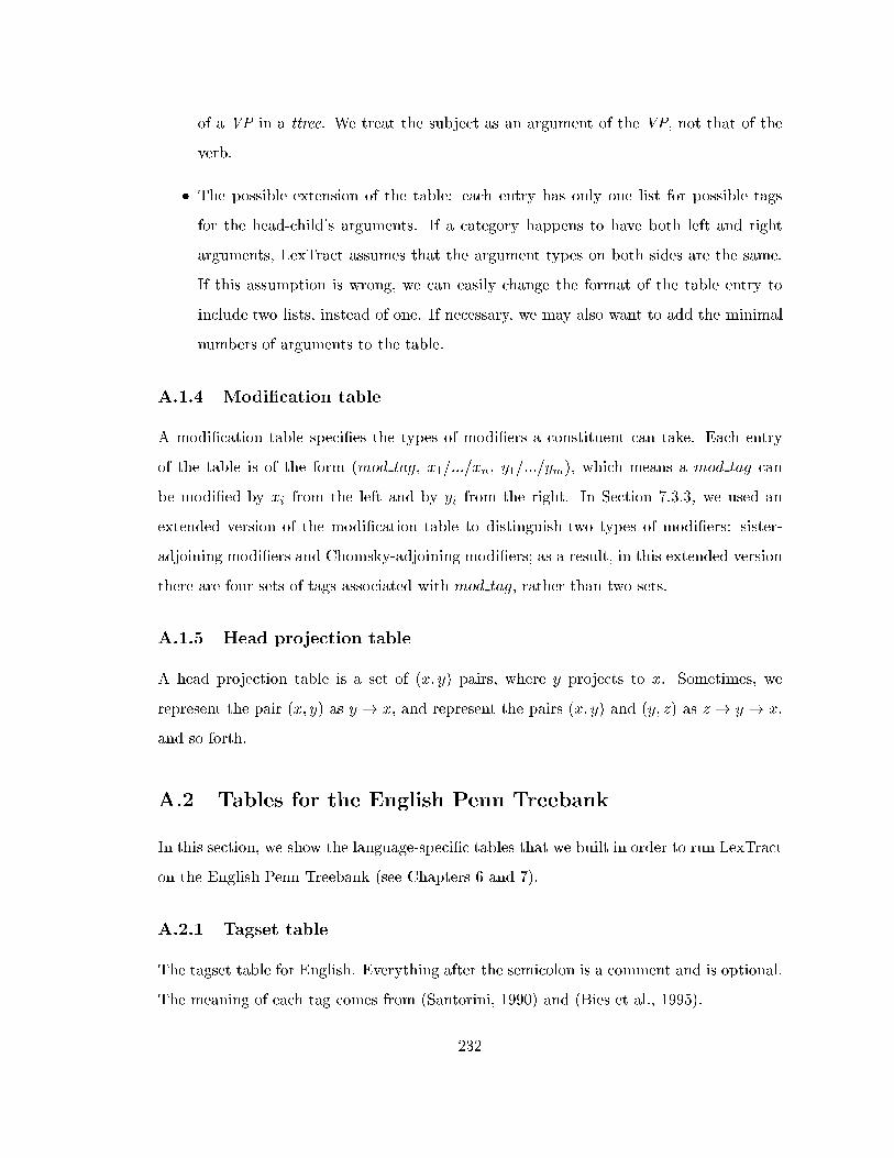
of a VP in a ttree. We treat the subject as an argument of the VP, not that of the
verb.
� The possible extension of the table: each entry has only one list for possible tags
for the head-child's arguments. If a category happens to have both left and right
arguments, LexTract assumes that the argument types on both sides are the same.
If this assumption is wrong, we can easily change the format of the table entry to
include two lists, instead of one. If necessary, we may also want to add the minimal
numbers of arguments to the table.
A.1.4 Modi�cation table
A modi�cation table speci�es the types of modi�ers a constituent can take. Each entry
of the table is of the form (mod tag, x1=:::=xn, y1=:::=ym), which means a mod tag can
be modi�ed by xi from the left and by yi from the right. In Section 7.3.3, we used an
extended version of the modi�cation table to distinguish two types of modi�ers: sister-
adjoining modi�ers and Chomsky-adjoining modi�ers; as a result, in this extended version
there are four sets of tags associated with mod tag, rather than two sets.
A.1.5 Head projection table
A head projection table is a set of (x; y) pairs, where y projects to x. Sometimes, we
represent the pair (x; y) as y ! x, and represent the pairs (x; y) and (y; z) as z ! y ! x,
and so forth.
A.2 Tables for the English Penn Treebank
In this section, we show the language-speci�c tables that we built in order to run LexTract
on the English Penn Treebank (see Chapters 6 and 7).
A.2.1 Tagset table
The tagset table for English. Everything after the semicolon is a comment and is optional.
The meaning of each tag comes from (Santorini, 1990) and (Bies et al., 1995).
232
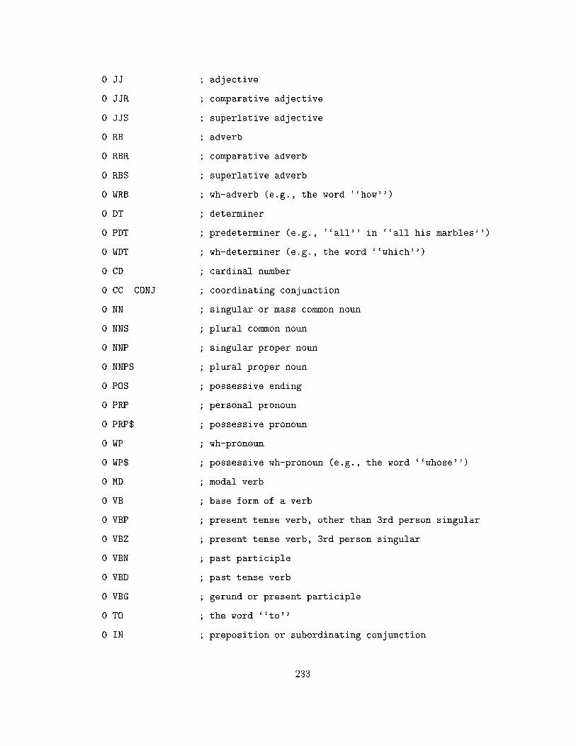
0 JJ ; adjective
0 JJR ; comparative adjective
0 JJS ; superlative adjective
0 RB ; adverb
0 RBR ; comparative adverb
0 RBS ; superlative adverb
0 WRB ; wh-adverb (e.g., the word ``how'')
0 DT ; determiner
0 PDT ; predeterminer (e.g., ``all'' in ``all his marbles'')
0 WDT ; wh-determiner (e.g., the word ``which'')
0 CD ; cardinal number
0 CC CONJ ; coordinating conjunction
0 NN ; singular or mass common noun
0 NNS ; plural common noun
0 NNP ; singular proper noun
0 NNPS ; plural proper noun
0 POS ; possessive ending
0 PRP ; personal pronoun
0 PRP$ ; possessive pronoun
0 WP ; wh-pronoun
0 WP$ ; possessive wh-pronoun (e.g., the word ``whose'')
0 MD ; modal verb
0 VB ; base form of a verb
0 VBP ; present tense verb, other than 3rd person singular
0 VBZ ; present tense verb, 3rd person singular
0 VBN ; past participle
0 VBD ; past tense verb
0 VBG ; gerund or present participle
0 TO ; the word ``to''
0 IN ; preposition or subordinating conjunction
233
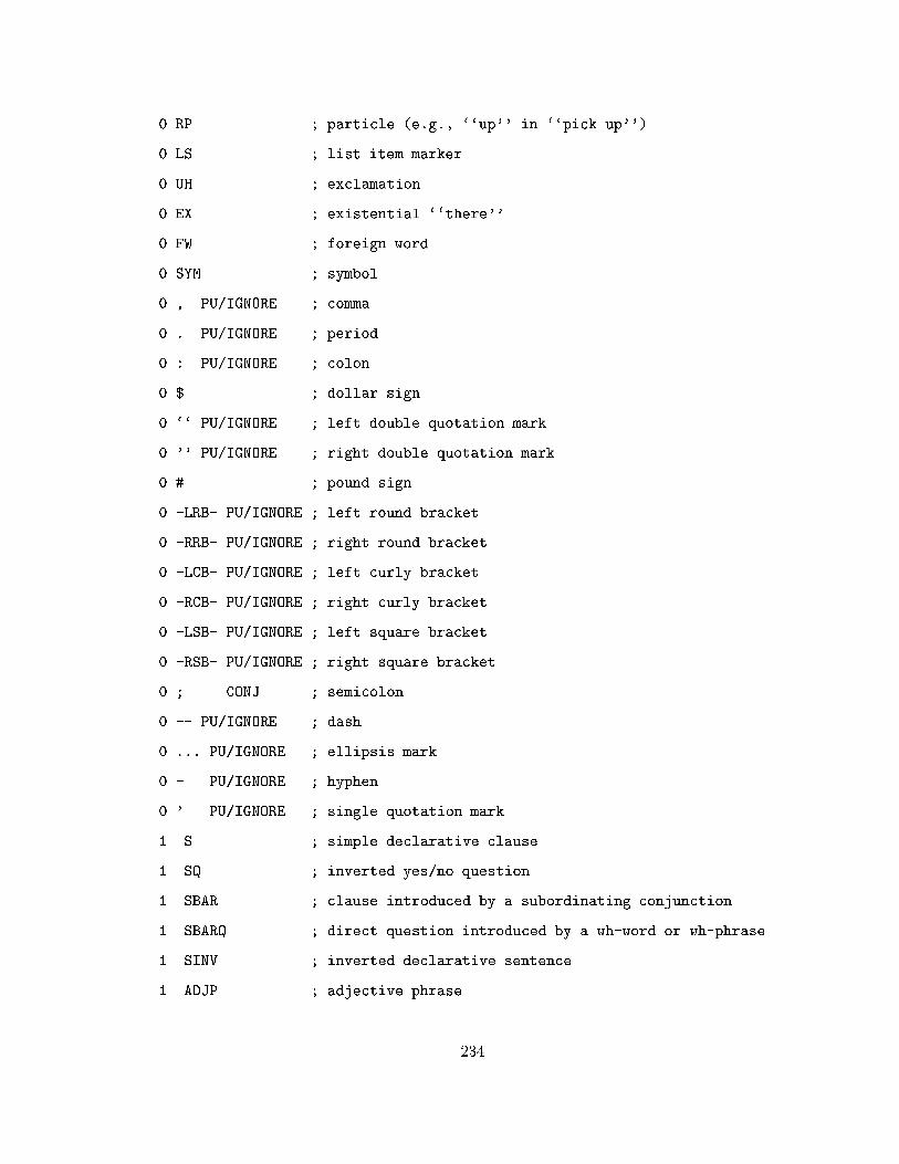
0 RP ; particle (e.g., ``up'' in ``pick up'')
0 LS ; list item marker
0 UH ; exclamation
0 EX ; existential ``there''
0 FW ; foreign word
0 SYM ; symbol
0 , PU/IGNORE ; comma
0 . PU/IGNORE ; period
0 : PU/IGNORE ; colon
0 $ ; dollar sign
0 `` PU/IGNORE ; left double quotation mark
0 '' PU/IGNORE ; right double quotation mark
0 # ; pound sign
0 -LRB- PU/IGNORE ; left round bracket
0 -RRB- PU/IGNORE ; right round bracket
0 -LCB- PU/IGNORE ; left curly bracket
0 -RCB- PU/IGNORE ; right curly bracket
0 -LSB- PU/IGNORE ; left square bracket
0 -RSB- PU/IGNORE ; right square bracket
0 ; CONJ ; semicolon
0 -- PU/IGNORE ; dash
0 ... PU/IGNORE ; ellipsis mark
0 - PU/IGNORE ; hyphen
0 ' PU/IGNORE ; single quotation mark
1 S ; simple declarative clause
1 SQ ; inverted yes/no question
1 SBAR ; clause introduced by a subordinating conjunction
1 SBARQ ; direct question introduced by a wh-word or wh-phrase
1 SINV ; inverted declarative sentence
1 ADJP ; adjective phrase
234

1 ADVP ; adverb phrase
1 CONJP ; conjunction phrase
1 FRAG ; fragment
1 INTJ ; interjection
1 LST ; list marker
1 NAC ; ``not a constituent'', used within a noun phrase
1 NP ; noun phrase
1 NX ; used within certain complex noun phrases
1 PP ; prepositional phrase
1 PRN PRN ; parenthetical
1 PRT ; particle
1 QP ; quantifier phrase
1 RRC ; reduced relative clause
1 UCP UCP ; unlike coordinated phrase
1 VP ; verb phrase
1 WHADJP ; wh-adjective phrase
1 WHADVP ; wh-adverb phrase
1 WHNP ; wh-noun phrase
1 WHPP ; wh-prepositional phrase
1 X ; unknown, uncertain, or unbracketable
2 -NONE- ; empty category
2 *T* BUILDMC ; trace of A'-movement
2 * ; arbitrary PRO, controlled PRO, and trace of A-movement
2 *NP* ; arbitrary PRO, controlled PRO
2 *PAS* ; trace of A-movement
2 *PPA* ; permanent predictable ambiguity
2 *U* ; unit
2 *NOT* ; anti-placeholder in template mapping
2 0 ; the null complementizer
2 *?* ELLIPSIS ; placeholder for ellipsed material
235

2 *RNR* BUILDMC ; right node raising
2 *ICH* BUILDMC ; ``interpret constituent here'' (discontinuous dependency)
2 *EXP* BUILDMC ; expletive (extraposition)
3 ADV ADJUNCT ; adverbial
3 NOM ; nominal
3 DTV ARGUMENT ; dative
3 LGS ; logical subject
3 PRD HEAD ; predicate
3 PUT ARGUMENT ; marks the locative complement of the word ``put''
3 SBJ ARGUMENT ; surface subject
3 TPC ADJUNCT ; topicalized element
3 VOC ADJUNCT ; vocative
3 BNF ; benefactive
3 DIR ADJUNCT ; direction
3 EXT ADJUNCT ; extent
3 LOC ADJUNCT ; locative
3 MNR ADJUNCT ; manner
3 PRP ADJUNCT ; purpose or reason
3 TMP ADJUNCT ; temporal
3 CLR ADJUNCT ; closely related
3 CLF ; cleft
3 HLN ; headline
3 TTL ; title
4 *T* ; trace of A'-movement
4 * ; arbitrary PRO, controlled PRO, and trace of A-movement
4 0 ; the null complementizer
4 *U* ; unit
4 *?* ; placeholder for ellipsed material
4 *NOT* ; anti-placeholder in template mapping
4 *RNR* ; right node raising
236

4 *ICH* ; ``interpret constituent here'' (discontinuous dependency)
4 *EXP* ; expletive (extraposition)
4 *PPA* ; permanent predictable ambiguity
A.2.2 Head percolation table
The head percolation table for English:
S right VP/SBAR/S
SINV right VP/SINV
SQ right VP/SQ
SBAR right S/SBAR/SINV
SBARQ right SQ/SBARQ
RRC right VP/RRC
NX right NX/NN/NNS/NNP/NNPS
NP right NP/NN/NNS/NNP/NNPS/NX/EX/CD/QP/JJ/JJR/JJS/PRP/DT/POS
NAC right NAC/NN/NNS/NNP/NNPS/NX
WHNP right WDT/WP/NP/NN/NNS/NNP/NNPS/NX/WHNP
QP right CD/QP
ADJP right JJ/JJR/VBN/ADJP/*?*
WHADJP right JJ/WHADJP
VP right VP/VB/VBN/VBP/VBZ/VBG/VBD/*?*
PP left IN/TO/VBG/PP
WHPP left IN/WHPP
ADVP right ADVP/RB/RBR/RBS/WRB
WHADVP right WRB/WHADVP
PRT right RP/PRT
INTJ left UH/INTJ
UCP right UCP
X right X
LST left LS
237
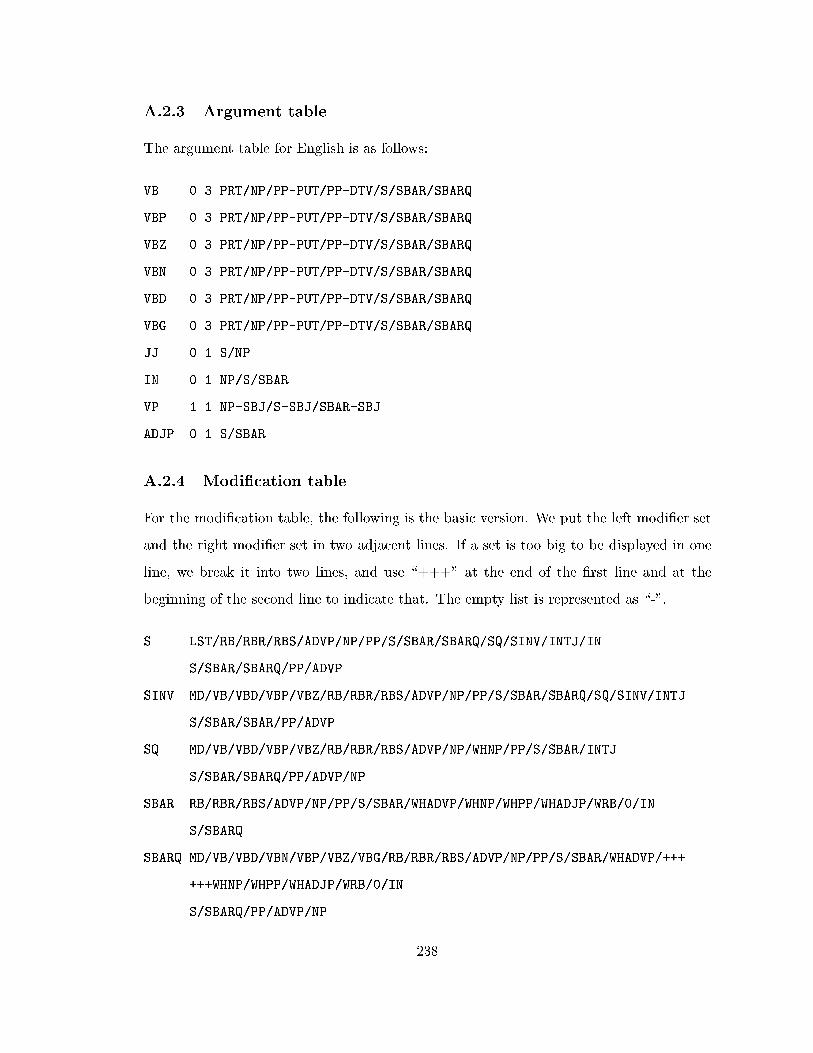
A.2.3 Argument table
The argument table for English is as follows:
VB 0 3 PRT/NP/PP-PUT/PP-DTV/S/SBAR/SBARQ
VBP 0 3 PRT/NP/PP-PUT/PP-DTV/S/SBAR/SBARQ
VBZ 0 3 PRT/NP/PP-PUT/PP-DTV/S/SBAR/SBARQ
VBN 0 3 PRT/NP/PP-PUT/PP-DTV/S/SBAR/SBARQ
VBD 0 3 PRT/NP/PP-PUT/PP-DTV/S/SBAR/SBARQ
VBG 0 3 PRT/NP/PP-PUT/PP-DTV/S/SBAR/SBARQ
JJ 0 1 S/NP
IN 0 1 NP/S/SBAR
VP 1 1 NP-SBJ/S-SBJ/SBAR-SBJ
ADJP 0 1 S/SBAR
A.2.4 Modi�cation table
For the modi�cation table, the following is the basic version. We put the left modi�er set
and the right modi�er set in two adjacent lines. If a set is too big to be displayed in one
line, we break it into two lines, and use \+++" at the end of the �rst line and at the
beginning of the second line to indicate that. The empty list is represented as \-".
S LST/RB/RBR/RBS/ADVP/NP/PP/S/SBAR/SBARQ/SQ/SINV/INTJ/IN
S/SBAR/SBARQ/PP/ADVP
SINV MD/VB/VBD/VBP/VBZ/RB/RBR/RBS/ADVP/NP/PP/S/SBAR/SBARQ/SQ/SINV/INTJ
S/SBAR/SBAR/PP/ADVP
SQ MD/VB/VBD/VBP/VBZ/RB/RBR/RBS/ADVP/NP/WHNP/PP/S/SBAR/INTJ
S/SBAR/SBARQ/PP/ADVP/NP
SBAR RB/RBR/RBS/ADVP/NP/PP/S/SBAR/WHADVP/WHNP/WHPP/WHADJP/WRB/0/IN
S/SBARQ
SBARQ MD/VB/VBD/VBN/VBP/VBZ/VBG/RB/RBR/RBS/ADVP/NP/PP/S/SBAR/WHADVP/+++
+++WHNP/WHPP/WHADJP/WRB/0/IN
S/SBARQ/PP/ADVP/NP
238
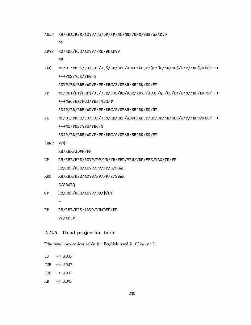
ADJP RB/RBR/RBS/ADVP/CD/QP/NP/NN/NNP/NNS/WRB/WHADVP
PP
ADVP RB/RBR/RBS/ADVP/WRB/WHADVP
PP
NAC NP/DT/PRP$/JJ/JJR/JJS/RB/RBR/ADVP/ADJP/QP/CD/NN/NNS/NNP/NNPS/NAC/+++
+++POS/VBN/VBG/$
ADVP/RB/RBR/ADVP/PP/RRC/S/SBAR/SBARQ/SQ/VP
NP NP/PDT/DT/PRP$/JJ/JJR/JJS/RB/RBR/ADVP/ADJP/QP/CD/NN/NNS/NNP/NNPS/+++
+++NAC/NX/POS/VBN/VBG/$
ADJP/RB/RBR/ADVP/PP/RRC/S/SBAR/SBARQ/SQ/NP
NX NP/DT/PRP$/JJ/JJR/JJS/RB/RBR/ADVP/ADJP/QP/CD/NN/NNS/NNP/NNPS/NAC/+++
+++NX/POS/VBN/VBG/$
ADJP/RB/RBR/ADVP/PP/RRC/S/SBAR/SBARQ/SQ/VP
WHNP WP$
RB/RBR/ADVP/PP
VP RB/RBR/RBS/ADVP/PP/MD/VB/VBD/VBN/VBP/VBZ/VBG/TO/VP
RB/RBR/RBS/ADVP/PP/NP/S/SBAR
RRC RB/RBR/RBS/ADVP/NP/PP/S/SBAR
S/SBARQ
QP RB/RBR/RBS/ADVP/CD/$/DT
-
PP RB/RBR/RBS/ADVP/WHADVP/PP
PP/ADVP
A.2.5 Head projection table
The head projection table for English used in Chapter 6.
JJ -> ADJP
JJR -> ADJP
JJS -> ADJP
RB -> ADVP
239
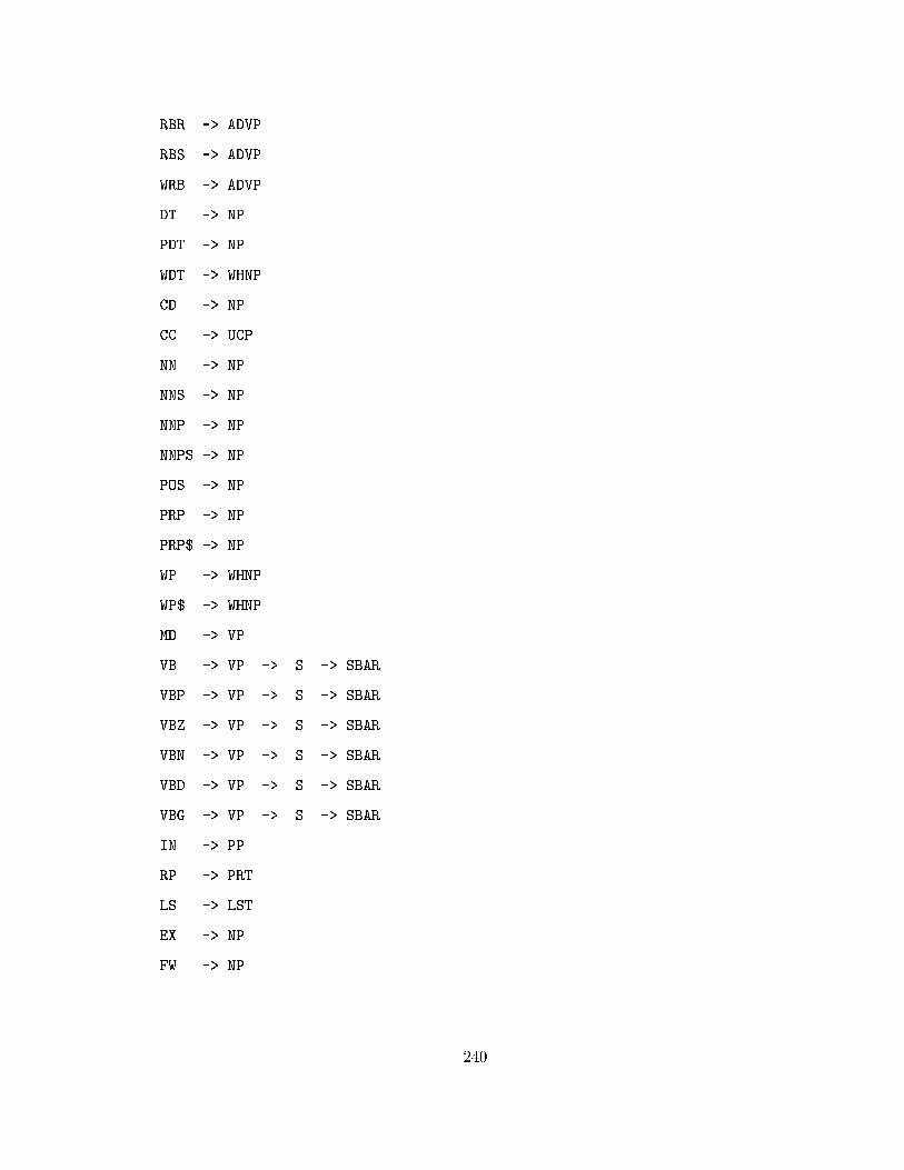
RBR -> ADVP
RBS -> ADVP
WRB -> ADVP
DT -> NP
PDT -> NP
WDT -> WHNP
CD -> NP
CC -> UCP
NN -> NP
NNS -> NP
NNP -> NP
NNPS -> NP
POS -> NP
PRP -> NP
PRP$ -> NP
WP -> WHNP
WP$ -> WHNP
MD -> VP
VB -> VP -> S -> SBAR
VBP -> VP -> S -> SBAR
VBZ -> VP -> S -> SBAR
VBN -> VP -> S -> SBAR
VBD -> VP -> S -> SBAR
VBG -> VP -> S -> SBAR
IN -> PP
RP -> PRT
LS -> LST
EX -> NP
FW -> NP
240
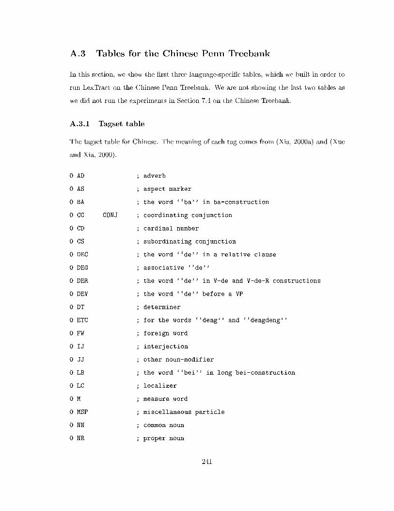
A.3 Tables for the Chinese Penn Treebank
In this section, we show the �rst three language-speci�c tables, which we built in order to
run LexTract on the Chinese Penn Treebank. We are not showing the last two tables as
we did not run the experiments in Section 7.4 on the Chinese Treebank.
A.3.1 Tagset table
The tagset table for Chinese. The meaning of each tag comes from (Xia, 2000a) and (Xue
and Xia, 2000).
0 AD ; adverb
0 AS ; aspect marker
0 BA ; the word ``ba'' in ba-construction
0 CC CONJ ; coordinating conjunction
0 CD ; cardinal number
0 CS ; subordinating conjunction
0 DEC ; the word ``de'' in a relative clause
0 DEG ; associative ``de''
0 DER ; the word ``de'' in V-de and V-de-R constructions
0 DEV ; the word ``de'' before a VP
0 DT ; determiner
0 ETC ; for the words ``deng'' and ``dengdeng''
0 FW ; foreign word
0 IJ ; interjection
0 JJ ; other noun-modifier
0 LB ; the word ``bei'' in long bei-construction
0 LC ; localizer
0 M ; measure word
0 MSP ; miscellaneous particle
0 NN ; common noun
0 NR ; proper noun
241
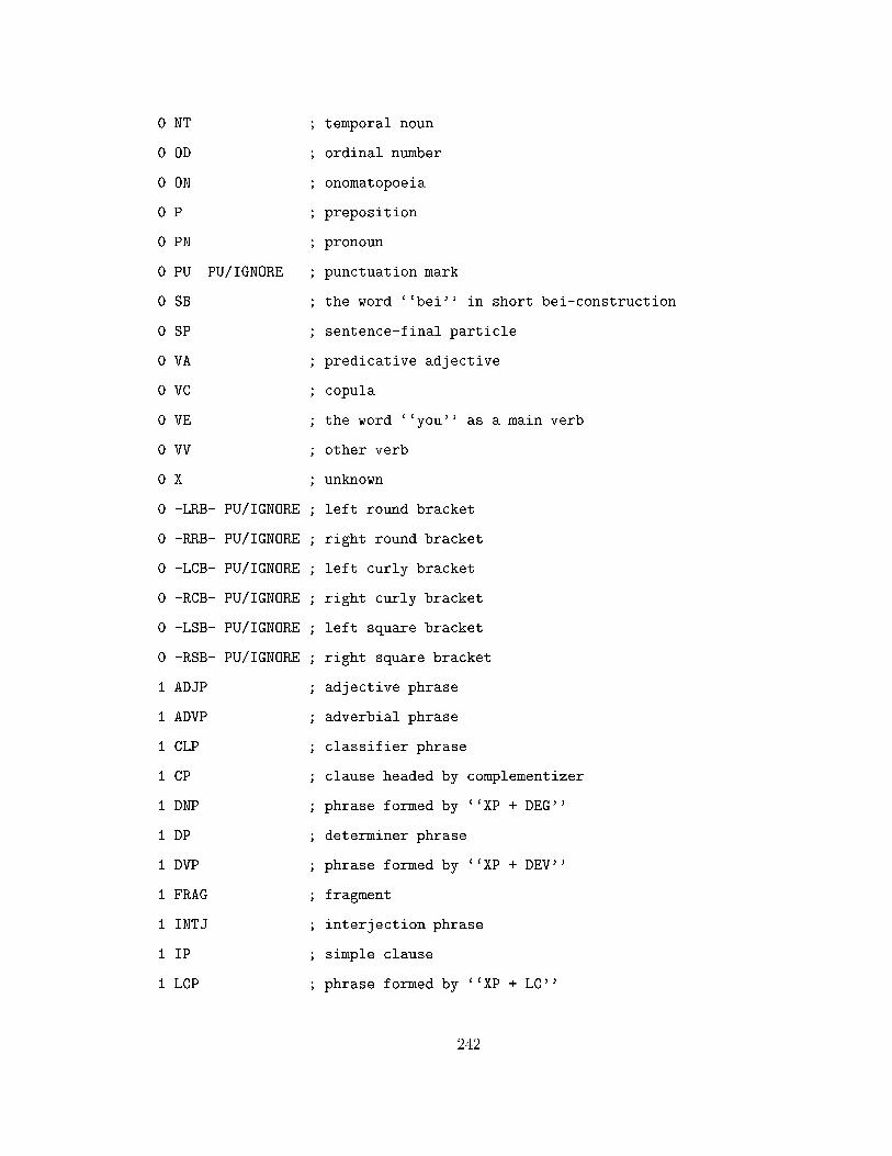
0 NT ; temporal noun
0 OD ; ordinal number
0 ON ; onomatopoeia
0 P ; preposition
0 PN ; pronoun
0 PU PU/IGNORE ; punctuation mark
0 SB ; the word ``bei'' in short bei-construction
0 SP ; sentence-final particle
0 VA ; predicative adjective
0 VC ; copula
0 VE ; the word ``you'' as a main verb
0 VV ; other verb
0 X ; unknown
0 -LRB- PU/IGNORE ; left round bracket
0 -RRB- PU/IGNORE ; right round bracket
0 -LCB- PU/IGNORE ; left curly bracket
0 -RCB- PU/IGNORE ; right curly bracket
0 -LSB- PU/IGNORE ; left square bracket
0 -RSB- PU/IGNORE ; right square bracket
1 ADJP ; adjective phrase
1 ADVP ; adverbial phrase
1 CLP ; classifier phrase
1 CP ; clause headed by complementizer
1 DNP ; phrase formed by ``XP + DEG''
1 DP ; determiner phrase
1 DVP ; phrase formed by ``XP + DEV''
1 FRAG ; fragment
1 INTJ ; interjection phrase
1 IP ; simple clause
1 LCP ; phrase formed by ``XP + LC''
242

1 LST ; list marker
1 NP ; noun phrase
1 PP ; preposition phrase
1 PRN PRN ; parenthetical
1 QP ; quantifier phrase
1 UCP UCP ; unlike coordinated phrase
1 VCD ; coordinated verb compound
1 VCP ; verb compounds formed by VV + VC
1 VNV ; verb compounds formed by A-not-A or A-one-A
1 VP ; verb phrase
1 VPT ; potential form V-de-R or V-bu-R
1 VRD ; verb resultative compound
1 VSB ; verb compounds formed by a modifier plus a head
1 WHNP ; wh-noun phrase
1 WHPP ; wh-preposition phrase
2 -NONE- ; empty category
2 *OP* ; operator
2 *pro* ; dropped argument
2 *PRO* ; arbitrary PRO, controlled PRO
2 *RNR* ; right node raising
2 *T* BUILDMC ; trace of A'-movement
2 *?* ELLIPSIS ; ellipsis
2 * ; trace of A-movement
3 FW ; foreign word
3 ADV ADJUNCT ; adverbial
3 APP ; appositive
3 BNF ; beneficiary
3 CND ; condition
3 DIR ; direction
3 EXT ; extent
243
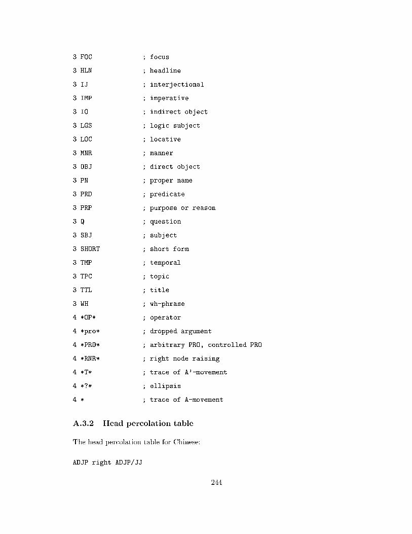
3 FOC ; focus
3 HLN ; headline
3 IJ ; interjectional
3 IMP ; imperative
3 IO ; indirect object
3 LGS ; logic subject
3 LOC ; locative
3 MNR ; manner
3 OBJ ; direct object
3 PN ; proper name
3 PRD ; predicate
3 PRP ; purpose or reason
3 Q ; question
3 SBJ ; subject
3 SHORT ; short form
3 TMP ; temporal
3 TPC ; topic
3 TTL ; title
3 WH ; wh-phrase
4 *OP* ; operator
4 *pro* ; dropped argument
4 *PRO* ; arbitrary PRO, controlled PRO
4 *RNR* ; right node raising
4 *T* ; trace of A'-movement
4 *?* ; ellipsis
4 * ; trace of A-movement
A.3.2 Head percolation table
The head percolation table for Chinese:
ADJP right ADJP/JJ
244
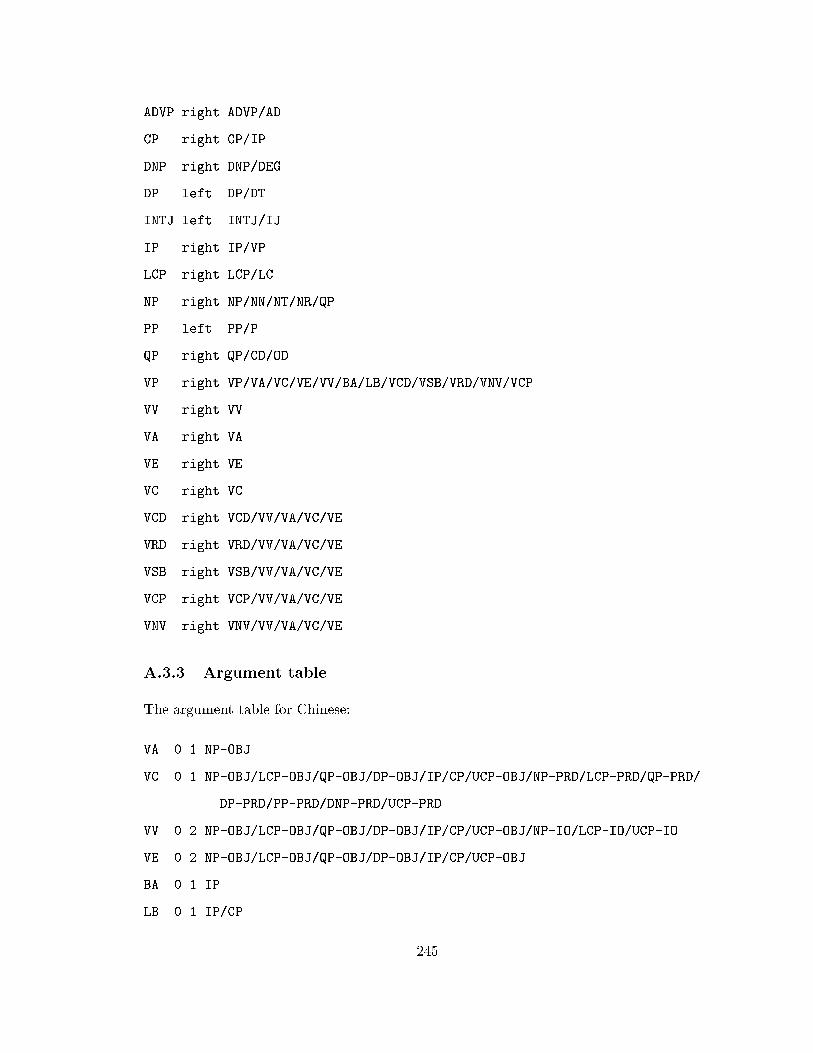
ADVP right ADVP/AD
CP right CP/IP
DNP right DNP/DEG
DP left DP/DT
INTJ left INTJ/IJ
IP right IP/VP
LCP right LCP/LC
NP right NP/NN/NT/NR/QP
PP left PP/P
QP right QP/CD/OD
VP right VP/VA/VC/VE/VV/BA/LB/VCD/VSB/VRD/VNV/VCP
VV right VV
VA right VA
VE right VE
VC right VC
VCD right VCD/VV/VA/VC/VE
VRD right VRD/VV/VA/VC/VE
VSB right VSB/VV/VA/VC/VE
VCP right VCP/VV/VA/VC/VE
VNV right VNV/VV/VA/VC/VE
A.3.3 Argument table
The argument table for Chinese:
VA 0 1 NP-OBJ
VC 0 1 NP-OBJ/LCP-OBJ/QP-OBJ/DP-OBJ/IP/CP/UCP-OBJ/NP-PRD/LCP-PRD/QP-PRD/
DP-PRD/PP-PRD/DNP-PRD/UCP-PRD
VV 0 2 NP-OBJ/LCP-OBJ/QP-OBJ/DP-OBJ/IP/CP/UCP-OBJ/NP-IO/LCP-IO/UCP-IO
VE 0 2 NP-OBJ/LCP-OBJ/QP-OBJ/DP-OBJ/IP/CP/UCP-OBJ
BA 0 1 IP
LB 0 1 IP/CP
245
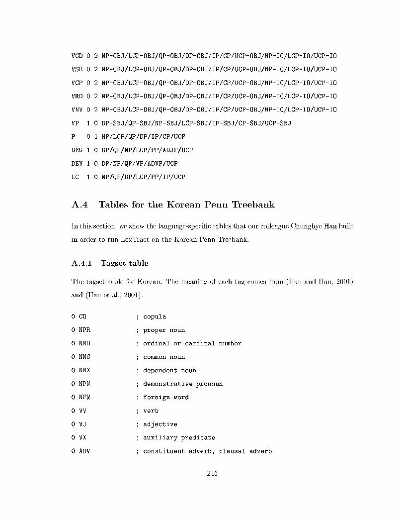
VCD 0 2 NP-OBJ/LCP-OBJ/QP-OBJ/DP-OBJ/IP/CP/UCP-OBJ/NP-IO/LCP-IO/UCP-IO
VSB 0 2 NP-OBJ/LCP-OBJ/QP-OBJ/DP-OBJ/IP/CP/UCP-OBJ/NP-IO/LCP-IO/UCP-IO
VCP 0 2 NP-OBJ/LCP-OBJ/QP-OBJ/DP-OBJ/IP/CP/UCP-OBJ/NP-IO/LCP-IO/UCP-IO
VRD 0 2 NP-OBJ/LCP-OBJ/QP-OBJ/DP-OBJ/IP/CP/UCP-OBJ/NP-IO/LCP-IO/UCP-IO
VNV 0 2 NP-OBJ/LCP-OBJ/QP-OBJ/DP-OBJ/IP/CP/UCP-OBJ/NP-IO/LCP-IO/UCP-IO
VP 1 0 DP-SBJ/QP-SBJ/NP-SBJ/LCP-SBJ/IP-SBJ/CP-SBJ/UCP-SBJ
P 0 1 NP/LCP/QP/DP/IP/CP/UCP
DEG 1 0 DP/QP/NP/LCP/PP/ADJP/UCP
DEV 1 0 DP/NP/QP/VP/ADVP/UCP
LC 1 0 NP/QP/DP/LCP/PP/IP/UCP
A.4 Tables for the Korean Penn Treebank
In this section, we show the language-speci�c tables that our colleague Chunghye Han built
in order to run LexTract on the Korean Penn Treebank.
A.4.1 Tagset table
The tagset table for Korean. The meaning of each tag comes from (Han and Han, 2001)
and (Han et al., 2001).
0 CO ; copula
0 NPR ; proper noun
0 NNU ; ordinal or cardinal number
0 NNC ; common noun
0 NNX ; dependent noun
0 NPN ; demonstrative pronoun
0 NFW ; foreign word
0 VV ; verb
0 VJ ; adjective
0 VX ; auxiliary predicate
0 ADV ; constituent adverb, clausal adverb
246

0 ADC CONJ ; conjunctive adverb
0 DAN ; configurative, demonstrative
0 IJ ; exclamation
0 LST ; list marker
0 LV ; light verb
0 CV ; complex verb
0 SCM PU/IGNORE ; comma
0 SFN PU/IGNORE ; sentence-ending punctuation (i.e., ``.'', ``?'', and ``!'')
0 SLQ PU/IGNORE ; left quotation mark
0 SRQ PU/IGNORE ; right quotation mark
0 SSY PU/IGNORE ; other punctuation mark
0 PQO ; complementizer
0 PAD ; adverbial postposition
0 PAU ; auxiliary adverbial postposition
0 PCA ; case postposition
0 PCJ ; conjective postposition
1 S ; simple sentential clause
1 ADJP ; adjective phrase
1 ADVP ; sentential and phrasal adverb phrase
1 ADCP ; coordinate adverb phrase
1 INTJ ; interjection
1 LST ; list marker
1 VP ; verb phrase
1 NP ; noun phrase
1 DANP ; adnominal phrase
1 PRN ; parenthetical
1 X ; unknown
1 WHNP ; wh-noun phrase
1 LVP ; light verb phrase
2 -NONE- ; empty category
247
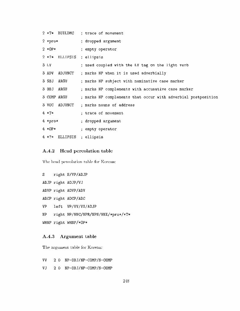
2 *T* BUILDMC ; trace of movement
2 *pro* ; dropped argument
2 *OP* ; empty operator
2 *?* ELLIPSIS ; ellipsis
3 LV ; used coupled with the LV tag on the light verb
3 ADV ADJUNCT ; marks NP when it is used adverbially
3 SBJ ARGU ; marks NP subject with nominative case marker
3 OBJ ARGU ; marks NP complements with accusative case marker
3 COMP ARGU ; marks NP complements that occur with adverbial postposition
3 VOC ADJUNCT ; marks nouns of address
4 *T* ; trace of movement
4 *pro* ; dropped argument
4 *OP* ; empty operator
4 *?* ELLIPSIS ; ellipsis
A.4.2 Head percolation table
The head percolation table for Korean:
S right S/VP/ADJP
ADJP right ADJP/VJ
ADVP right ADVP/ADV
ADCP right ADCP/ADC
VP left VP/VV/VX/ADJP
NP right NP/NNC/NPR/NPN/NNX/*pro*/*T*
WHNP right WHNP/*OP*
A.4.3 Argument table
The argument table for Korean:
VV 2 0 NP-OBJ/NP-COMP/S-COMP
VJ 2 0 NP-OBJ/NP-COMP/S-COMP
248

VP 3 0 NP-SBJ/S-SBJ/NP-OBJ/NP-COMP/S-COMP/S-OBJ
ADJP 1 0 NP-OBJ/NP-COMP/S-COMP/S-OBJ
S 2 0 NP-OBJ/NP-COMP/S-COMP/S-OBJ/WHNP
249

Appendix B
Building a high-quality Treebank
Treebanks are a prerequisite for running LexTract and training any supervised NLP tools
such as POS taggers and parsers. It is well-known that building a large high-quality Tree-
bank is very challenging. In this appendix, we want to address the following question:
how to best build a high-quality Treebank from scratch? The discussion on this issue is
mainly based on my experience as the project manager and one of the guideline designers
of the Chinese Penn Treebank Project (Xia et al., 2000b) and as a user of various Tree-
banks including the three Penn Treebanks. Instead of examining each aspect of Treebank
development, we shall concentrate on the following three topics.
Guideline preparation: Preparing good guidelines is never easy, and doing so for Chi-
nese is even more diÆcult because of certain characteristics of Chinese, which we
shall discuss in Section B.2.
Quality control: We have explored various methods to improve inter-annotator consis-
tency and annotation accuracy.
The role of NLP tools: It is well-known that using NLP tools (e.g., POS taggers and
parsers) for preprocessing can reduce human annotation time. In this appendix, we
shall show that they can also be used for guideline preparation and quality control.
Although our approach was aimed at solving problems that we encountered in the
Chinese Penn Treebank Project, we believe that our methodology is general enough to
250
be applied to text annotation for other languages as well. This appendix is organized as
follows: in Section B.1, we give an overview of the Chinese Penn Treebank Project; in
Section B.2, we describe the methodology for guideline preparation; in Section B.3 | B.5,
we highlight the challenges encountered while making three sets of guidelines; in Section
B.6, we discuss a strategy for quality control; in Section B.7, we explore various ways that
NLP tools are used to speed up annotation and to improve the quality of the Treebank. in
Section B.8, we address the similarities and di�erences between Treebank guidelines and
hand-crafted grammars.
B.1 Overview of the Chinese Penn Treebank Project
The on-going Chinese Penn Treebank Project started in late 1998. The goal of the project
is to build a large-scale high-quality Treebank for Chinese. The �rst portion of the Tree-
bank, which has about 100 thousand words, was released to the public in December 2000.
Since then, more data from various sources have been annotated. In this appendix, by
the Treebank, we mean this 100-thousand-word portion of the Treebank unless speci�ed
otherwise.
The Treebank consists of 325 articles from the Xinhua newswire published in 1994-
1998.1 It contains 172 thousand hanzi (Chinese characters), or 100 thousand words after
word segmentation. The corpus has 4183 sentences, averaging 41 hanzi (or 23.8 words
after segmentation) per sentence.2 A preliminary version of the Treebank was released to
the public in June 2000, and the �nal version was released in December 2000.
Our team includes two linguistics professors, three computational linguists, two anno-
tators (both are linguistics graduate students) and several external consultants. As the
project manager and one of the guideline designers, my responsibilities include writing
word segmentation and POS tagging guidelines, co-authoring bracketing guidelines, de-
signing strategies for quality control, organizing weekly meetings and leading discussions
1The majority of these documents focus on economic developments, while the rest describe general
political and cultural topics.2A sentence is anything that ends with a period, a exclamation mark or a question mark. We also treat
the headline of each article as a sentence.
251
with a group of linguists, organizing a number of workshops and meetings in USA and
abroad, and so on.
B.1.1 Project inception
With growing interest in Chinese Language Processing, numerous NLP tools (e.g., word
segmenters, POS taggers, and parsers) for Chinese have been developed all over the world.
However, when we started the project in late 1998, there were no large-scale Chinese
Treebanks available to the public; as a result, it was diÆcult to compare results and gauge
progress in the �eld.
To assess community interest in a Chinese Treebank, we organized a three-day work-
shop on Chinese language processing at the University of Pennsylvania in June 1998. The
aim of this workshop was to bring together in uential researchers from mainland China,
Hong Kong, Taiwan, Singapore, and the United States in a move towards consensus build-
ing with respect to word segmentation, POS tagging, syntactic bracketing and other areas.3
The workshop included presentations of guidelines that were used in mainland China and
Taiwan, as well as segmenters, POS taggers and parsers. There were also several work-
ing groups that discussed speci�c issues in segmentation, POS tagging and the syntactic
annotation of newswire text.
There was general consensus at this workshop that an e�ort to create a large-scale
Chinese Treebank would be well-received, and that linguistics expertise was a necessary
prerequisite to successful completion of such a project. The workshop made considerable
progress in de�ning criteria for segmentation guidelines as well as addressing the issues of
POS tagging and syntactic bracketing. The Chinese Penn Treebank Project began shortly
after the workshop.4
3The American groups included the Institute for Research in Cognitive Science and the Linguistics Data
Consortium (which distributes the English Treebank) at the University of Pennsylvania, the University of
Maryland, Queens College, the University of Kansas, the University of Delaware, Johns Hopkins University,
New Mexico State University, Systran, BBN Technology, AT & T, Lucent Technology, Xerox, West, Unisys
and the US Department of Defense. We also invited scholars from mainland China, Taiwan, Hong Kong
and Singapore.4Our Chinese Penn Treebank website, http://www.ldc.upenn.edu/ctb, includes segmentation, POS tag-
ging and bracketing guidelines, as well as sample �les, information on two Chinese Language Processing
252

B.1.2 Annotation process
The annotation was done in two phases: the �rst phase was word segmentation and POS
tagging, and the second phase was syntactic bracketing. At each phase, all the data
were annotated at least twice with a second annotator correcting the output of the �rst
annotator. During the process, we held several meetings to get feedback from the Chinese
NLP community and revised our guidelines accordingly. Figures B.1 and B.2 summarize
the milestones of the project. Throughout the project, we also used various NLP tools to
speed up and improve the quality of the annotation (see Section B.7 for details).
workshops and meetings
guidelines and annotations
6/98 8/98 9/98 11/98 1/99 3/99
finish
1st
draf
t
Beijing, ChinaICCIP-98meeting during
CanadaMontrealACL-98meeting during
USAPhiladelphiaworkshop3-day CLP
start
1st p
ass
finish
2nd
dra
ft
finish
1st
pass
start
2nd
pass
finish
2nd
pas
s
com
pile
lexico
n
and
clean
the
corp
us
"draft": draft of word segmentation and POS tagging guidelines
"pass": segmenting and POS tagging the corpus
Figure B.1: The �rst phase: segmentation and POS tagging
final
clean
up
finish
1st
draf
t
start
1st p
ass
finish
1st
pass
finish
2nd
dra
ft
start
2nd
pass
finish
2nd
pas
s
finali
ze g
uideli
nes
extra
ct gr
amm
ars
workshops and meetings
5/99 12/99
guidelines and annotations
release of the Treebank
"draft": draft of bracketing guidelines
"pass": bracketing the corpus
4/00 6/00
prelim release
9/00
Hong Kongworkshop2nd CLP
10/00 12/00
2nd release
6/99meeting duringACL-99Maryland, USA
10/99
Figure B.2: The second phase: bracketing and data release
workshops and much more.
253

B.2 Methodology for guideline preparation
To build a Chinese Treebank we need three sets of guidelines | word segmentation, part-
speech tagging and bracketing guidelines. Making these guidelines for Chinese is especially
challenging because of the following characteristics of Chinese.
� Unlike Western writing systems, Chinese writing does not have a natural delimiter
between words, and the notion of word is very hard to de�ne.
� Chinese has very little, if any, in ectional morphology. Words are not in ected with
number, gender, case, or tense. For example, a word such as hu��-mi�e in Chinese
corresponds to destroy/destroys/destroyed/destruction in English. This fuels the dis-
cussion in Chinese NLP communities on whether the POS tags should be based on
meaning or on syntactic distribution. If only the meaning is used, hu��-mi�e should be
a verb all the time. If syntactic distribution is used, the word is either a verb or a
noun according to the context.
� There are many open questions in Chinese syntax. To further complicate the sit-
uation, Chinese, like any other language, is under constant change. With its long
history, a seemingly homogeneous phenomenon in Chinese (such as long and short
bei-construction) may be, in fact, a set of historically related but syntactically inde-
pendent constructions (Feng, 1998).
� Chinese is widely spoken in areas as diverse as mainland China, Hong Kong, Taiwan,
and Singapore. There is a growing body of research in Chinese natural language
processing, but little consensus on linguistic standards along the lines of the EAGLES
initiative in Europe.5
To tackle these issues, we adopted the following approach:
� In addition to studying the literature on Chinese morphology and syntax, we collab-
orated closely with our linguistics experts to work out plausible analyses for syntactic
constructions.5EAGLES stands for the Expert Advisory Group on Language Engineering Standards. For more infor-
mation, please check out its website at http://www.ilc.pi.cnr.it/EAGLES/home.html.
254
� When there were no clear winners among several alternatives, we chose one, and
annotated the corpus in a way that our annotation could be easily converted to
accommodate other alternatives when needed.
� We studied other groups' standards or guidelines, such as the Segmentation Standard
in mainland China (Liu et al., 1993) and the one in Taiwan (Chinese Knowledge
Information Processing Group, 1996), and accommodated them in our guidelines if
possible.
� We organized regular workshops and meetings and invited experts from the United
States and abroad to discuss open questions, share resources and seek consensus. We
also visited mainland China, Hong Kong, and Taiwan to present our work and ask
for feedback.
� Annotators were encouraged to ask questions during the annotation process, and
in the second pass of bracketing randomly selected �les were re-annotated by both
annotators to evaluate their consistency and accuracy. Annotation errors and inter-
annotator inconsistencies revealed places in the guidelines that needed revision.
In an ideal situation, guidelines should be �nalized before annotation begins. However,
the raw data from a Treebank are far more complicated and subtle than the examples
discussed in the linguistics literature. Many problems do not surface until suÆcient data
have been studied. In this project, we divided each phase of the annotation and guideline
development into several steps:
1. Before the �rst pass, we created the �rst version of guidelines based on corpus anal-
ysis, review of the literature, and consultation with experts in Treebanking and
Chinese linguistics.
2. During the �rst pass, these guidelines evolved gradually through the resolution of
annotation diÆculties and annotator inconsistencies.
3. After the �rst pass, the guidelines were partially �nalized and when possible the
corpus was automatically converted to be consistent with the new guidelines before
the second pass began;
255
4. In the second pass, we applied our quality control method (see Section B.6) to detect
places in the guidelines that needed revision. Fortunately, very little revision at this
stage was needed.
5. After the second pass, the guidelines were �nalized and the annotation was revised
if necessary.
In this process, through careful design of the �rst version of the guidelines, no sub-
stantial changes were made in the following versions and most revision of the annotation
was done automatically by simple conversion tools. In the next three sections, we discuss
highlights from each set of guidelines.
B.3 Segmentation guidelines
The central issue for word segmentation is how the notion of word should be de�ned.
B.3.1 Notions of word
There are many di�erent notions of words. Sciullo andWillams (1987) discuss four of them;
namely, morphological object, syntactic atom, phonological word and listeme. According
to (Sciullo and Williams, 1987), the syntactic atoms are the primes of syntax. They
possess the syntactic atomicity properties; that is, the inability of syntactic rules to analyze
the contents of X0 categories.6 Packard (2000) de�nes eight notions of word; namely,
orthographic word, sociological word, lexical word, semantic word, phonological word,
morphological word, syntactic word, and psycholinguistic word. Because our goal was to
build syntactic structures for sentences, we adopted the notion syntactic word (or syntactic
atom in (Sciullo and Williams, 1987)) for our word segmentation task.7
6Whether morphology and syntax are truly independent is still an open question (Sciullo and Williams,
1987). We shall not go into details in this thesis.7In the word segmentation and POS tagging phase, we broke the sentences into segments. Most segments
are syntactic words, but we treat certain bound morphemes (such as aspect markers) as segments to make
the Treebank more compatible with several widely used standards in the Chinese NLP community.
256

Once the notion of word is de�ned, the notions of aÆx, bound morpheme, compound
and phrase can be de�ned accordingly. However, the distinction between a word and a non-
word is not always clear-cut. For example, in English, the morpheme pro- (which means
supporting) cannot be used alone; therefore, it looks like a bound morpheme. However,
it can appear in a coordinated structure, such as pro- and anti-abortion. Based on the
assumption that only words and phrases can be coordinated, it behaves like a word.8
Therefore, the status of pro- is somewhere between a bound morpheme and a word. Making
the word and non-word distinction is even more diÆcult for Chinese for a number of
reasons:
� Chinese is not written with word delimiters, so segmenting a sentence into "words"
is not a natural task even for a native speaker.
� Chinese has little in ectional morphology to ease the word segmentation problem.
� The structures within words and phrasal structures are similar in many cases, making
the distinction between words and phrases more elusive.
� There is little consensus in the community on the treatment of some constructions
that could a�ect word segmentation. For example, there are two competing views for
verb resultatives (e.g., chu��-g�an/blow-dry). One view believes that a verb resultative
is formed in the lexicon, and therefore should be one word; whereas the other view
says that a simple sentence with a verb resultative is actually bi-clausal and the verb
resultative is formed by movement; therefore, it should be treated as two words.
� Many monosyllabic morphemes that used to be able to stand alone become bound
in Modern Chinese. The in uence of non-Modern Chinese makes it diÆcult to draw
the line between bound morphemes and free morphemes, the notions which could
otherwise have been very useful for deciding word boundaries.
Not surprisingly, the de�nition of word in Chinese has been notoriously controversial
in the Chinese linguistic community; as a result, the word standards adopted by various
8For example, both a- and im- are bound morphemes and \amoral and immoral" cannot be shortened
into \a- and immoral".
257

research groups, including the national standard in mainland China (Liu et al., 1993) and
the word standard used by the Academia Sinica in Taiwan (Chinese Knowledge Information
Processing Group, 1996), di�er substantially.
B.3.2 An experiment
To test how well native speakers agree on word segmentation of written texts, we randomly
chose 100 sentences (5060 hanzi) from the Xinhua newswire and asked the participants of
the �rst Chinese Language Processing (CLP) workshop to segment the sentences according
to their personal preferences.9 We got replies from seven groups, almost all of whom hand
corrected their output before sending the results to us. Table B.1 shows the results of
comparing the output between each group pair. Here, we use three measures that are
commonly used to measure parsing accuracy: precision, recall, and the number of crossing
brackets (Black et al., 1991).10
The experiment was similar to the one discussed in (Sproat et al., 1996) in which six
native speakers were asked to mark all the places they might pause if they were reading the
text aloud. In both experiments, the native speakers (or judges) were not given any speci�c
segmentation guidelines. Following (Sproat et al., 1996), we calculated the arithmetic
mean of the precision and the recall as the measure of agreement between each output
9We did not give them any segmentation guidelines. Some participants applied their own standards for
which they had automatic segmenters, while others simply followed their intuitions.10Given a candidate �le and a Gold Standard �le, the three metrics are de�ned as: the precision is
the number of correct constituents in the candidate �le divided by the number of constituents in the
candidate �le, the recall is the number of correct constituents in the candidate �le divided by the number
of constituents in the Gold Standard �le, and the number of crossing brackets is the number of constituents
in the candidate �le that cross a constituent in a Gold Standard �le.
If we treat each word as a constituent, a segmented sentence is similar to a bracketed sentence whose
depth is one. To compare two outputs, we chose one as the Gold Standard, and evaluated the other output
against it. As noted in (Sproat et al., 1996), for two outputs J1 and J2, taking J1 as the Gold Standard and
computing the precision and recall for J2 yields the same results as taking J2 as the Gold Standard and
computing the recall and the precision respectively for J1. However, the number of crossing brackets when
J1 is the Gold Standard is not the same as when J2 is the Gold Standard. For example, if the string is
ABCD and J1 segments it into AB CD and J2 marks it as A BC D, then the number of crossing brackets
is 1 if J1 is the Gold Standard and the number is 2 if J2 is the Gold Standard.
258

1 2 3 4 5 6 7 average
1 - 90/88/6 90/90/4 83/88/3 92/91/3 91/91/3 92/84/9 90/89/5
2 88/90/3 - 87/90/3 80/88/14 89/90/4 86/89/3 89/83/7 87/88/6
3 90/90/3 90/87/5 - 82/88/2 89/88/5 89/89/4 89/82/10 88/87/5
4 88/83/9 88/80/10 88/82/7 - 92/86/7 86/81/9 87/74/16 88/81/10
5 91/92/3 90/89/4 88/89/4 86/92/9 - 90/90/4 92/85/8 90/90/5
6 91/91/3 89/86/6 89/89/4 81/86/3 90/90/4 - 91/83/10 89/88/5
7 84/92/1 83/89/2 82/89/2 74/87/4 85/92/1 83/91/1 - 82/90/2
Table B.1: Comparison of word segmentation results from seven groups
pair. The average agreement in our experiment was 87.6%, much higher than 76% in
(Sproat et al., 1996). Without comparing the raw text used in these two experiments,
we do not know for sure why the numbers di�ered so much. One factor that might have
contributed to the di�erence is that the instructions given to the judges were not exactly
the same: in our experiment, the judges were asked to segment the sentences into words
according to their own de�nitions of word, whereas in their experiment, the judges were
asked to mark all places they might possibly pause if they were reading the text aloud.
There are places in Chinese { for example, between a verb and the aspect marker that
follows the verb { where native speakers do not pause, but they still treat the verb and
the aspect marker as two words. Another factor that might explain why the degree of the
agreement in our experiment was much higher is that in our experiment all the judges were
well-trained computational linguists. Some judges had their own segmentation guidelines
and/or segmenters. They either followed their guidelines or used their segmenters to
automatically segment the data and then hand corrected the output. Either way, their
outputs may be more consistent than the output of an average native speaker.
The fact that the average agreement in our experiment was 87.6% and the highest
agreement among all the pairs was 91.5% con�rms the belief that, without a set of seg-
mentation guidelines, native speakers often disagree on where word boundaries should be.
On the other hand, in our experiment the average number of crossing brackets between
each pair for the whole 100 sentences was only 5.4. Furthermore, most of these crossing
brackets were caused by careless human errors. This implies that much of the disagree-
ment was not critical and if the judges had been given good segmentation guidelines, the
agreement between them should have improved greatly.
259
B.3.3 Tests of wordness
Now that we have decided to use the notion of syntactic words for word segmentation, the
next task is to come up with a set of tests for establishing word boundaries. The following
tests have been proposed in the literature: (Without loss of generalization, we assume the
string that we are trying to segment is X-Y, where X and Y are two morphemes)
� Bound morpheme: a bound morpheme should be attached to its neighboring mor-
pheme to form a word when possible.
� Productivity: if the rule that combines the expression X-Y is not productive, then
X-Y is likely to be a word.
� Frequency of co-occurrence: if the expression X-Y occurs very often, it is likely to
be a word.
� Complex internal structure: strings with complex internal structures should be seg-
mented when possible.
� Compositionality: if the meaning of X-Y is not compositional, it is likely to be a
word.
� Insertion: if another morpheme can be inserted between X and Y, then X-Y is
unlikely to be a word.
� XP-substitution: if a morpheme cannot be replaced by a phrase of the same type,
then it is likely to be part of a word.
� The number of syllables: several guidelines (Liu et al., 1993; Chinese Knowledge
Information Processing Group, 1996) use syllable numbers on certain cases. For ex-
ample, in (Liu et al., 1993), a verb resultative is treated as one word if the resultative
part is monosyllabic, and it is treated as two words if the resultative part has more
than one syllable.
Notice that these tests are aimed at di�erent notions of head. For instance, the com-
positionality test is related to the notion of semantic word, whereas the XP-substitution
260

test is more relevant to syntactic word. Furthermore, none of these tests is suÆcient by
itself for covering the entire range of diÆcult cases. Either the test is applicable only to
limited cases (e.g., the XP-substitution test) or there is no objective way to perform the
test as the test refers to vaguely de�ned properties (e.g., in the productive test, it is not
clear where to draw the line between a productive rule and a non-productive rule). For
more discussion on this topic from the linguistics point of view, please refer to (Sciullo and
Williams, 1987; Packard, 1998; Packard, 2000).
Because the segments in our Treebank roughly correspond to syntactic words, we always
apply the tests for syntactic words (e.g., the XP-substitution test) �rst. If these tests are
not suÆcient, the tests for other notions of word are used. The rationale behind this
decision is that, although various notions of word di�er in their de�nitions and applicable
�elds, in most cases these notions of word do coincide with one another.11 Rather than
having the annotators memorize and apply these tests themselves, in the guidelines we
spell out what the results of applying the tests would be for all of the relevant phenomena.
For example, for the treatment of verb resultatives, we select the relevant tests (in this case
the number of syllables and the insertion test), and give several examples of the results of
applying these tests to the verb resultatives. This approach makes it straightforward, and
thus eÆcient, for the annotators to follow the guidelines.
The guidelines are organized according to the internal structure of the corresponding
expressions (e.g., a verb resultative is represented as V+V, whereas a verb-object form is
represented as V+N), so it is easy for the annotators to search the guidelines for reference.
The complete segmentation guidelines, including the comparisons between our guidelines
and the ones used in mainland China and Taiwan, can be found in (Xia, 2000b).
11For example, Packard (2000) de�nes a morphological word as the output of word-formation rules in
the language, and a syntactic word as a form that can stand as an independent occupant of a syntactic
form class slot. He also shows that mi�ao-t�ou/cat-head is a morphological word, but not a syntactic word.
Nevertheless, most morphological words are syntactic words and vice versa.
261

B.4 POS tagging guidelines
The central issue on POS tagging is how POS tags should be de�ned and distinguished
from one another.
B.4.1 Criteria for POS tagging
People generally agree that a POS tagset for Chinese should include the tags for nouns,
verbs, prepositions, adverbs, conjunctions, determiners, classi�ers, and so on, but they
di�er in how these tags should be de�ned. Because Chinese has little, if any, in ectional
morphology, the de�nition of a POS tag is based on either semantics or syntax. The �rst
view believes that the tags should be de�ned based on meaning, whereas the second one
de�nes POS tags based on syntactic distribution. As mentioned before, a word such as hu��-
mi�e in Chinese can be translated into destroy/destroys/destroyed/destroying/destruction
in English, and it is used roughly the same way as its counterparts in English. According
to the �rst view, POS tags should be based solely on meaning. Because the meaning of
the word remains roughly the same across all of these usages, the word should always be
tagged as a verb. The second view claims that POS tags should be determined by the
syntactic distribution of the word. When hu��-mi�e is the head of a noun phrase, it should
be tagged as a noun in that context. Similarly, when it is the head of a verb phrase, it
should be tagged as a verb. These two competing views have been under debate since the
1950s (Gong, 1997) and the controversy remains.
We choose syntactic distribution as our main criterion for POS tagging, because this
approach complies with the principles adopted in contemporary linguistics theories (such
as the notion of head projections in X-bar theory and GB theory) and it captures the
similarity between Chinese and other languages. One argument that is often used against
this approach is as follows: because many verbs in Chinese can also occur in noun positions,
using this approach will require these verbs to have two tags, thus increasing the size of the
lexicon. We �nd this argument not convincing. First, many verbs (such as monosyllabic
verbs) cannot occur in noun positions. The extra POS tag allows us to distinguish the
verbs that can occur in noun positions from the ones that cannot. Second, if there are
262

generalizations about what verbs can occur in noun positions and what cannot, these
generalizations can be represented as morphological rules, which allows the lexicon to
be expanded automatically. On the other hand, if no such generalizations exist and the
nominalization process is largely idiosyncratic, it supports the view that verbs that can
be nominalized should be marked by having two POS tags in the lexicon. Third, the
phenomenon that many verbs can also occur in noun positions is not unique to Chinese,
and the standard treatment in other languages is to give them both tags.
B.4.2 Choice of a POS tagset
Once we have decided that the POS tagging should be based on syntactic distribution of
words, the next step is choosing a POS tagset and then �nding tests to distinguish each
pair of POS tags in the tagset. The annotators then use the tests to tag the words in the
Treebank.
The syntactic distribution of a word can be seen as a set of positions at which the word
can appear, such as the argument position of a VP, the head of a VP and so on. The task
of choosing a tagset and tagging a corpus with the tagset can be stated as follows (see
Figure B.3):
Given the set of wordsW , a set of positions P , and a relation f � f(w; p) j w 2W;p 2 Pg, �nd a set of POS tags T , a relation f1 � f(w; t) j w 2 W; t 2 Tg,and a relation f2 � f(t; p) j t 2 T; p 2 Pg, such that f is a subset of f1 Æ f2.12
In this representation, f speci�es the positions in which the words in W can appear, f1
gives all possible POS tags of a word, and f2 speci�es the positions in which each POS
tag can appear. Once T , f1, and f2 are de�ned, any pair (t1; t2) of POS tags can be
distinguished by comparing the sets of positions in which t1 and t2 can appear. To tag a
word w in a sentence, the annotator �rst decides the position p of the word in the sentence,
then chooses a tag t such that (w; t) 2 f1 and (t; p) 2 f2.
Given W , P and f , it is obvious that the choice of T , f1 and f2 is not unique. For the
purpose of Treebank annotation, we prefer the following measures to be small:12f1 Æ f2 is the composition of two relations; that is, (x; y) 2 f1 Æ f2 if and only if there exists z such that
(x; z) 2 f1 and (z; y) 2 f2.
263
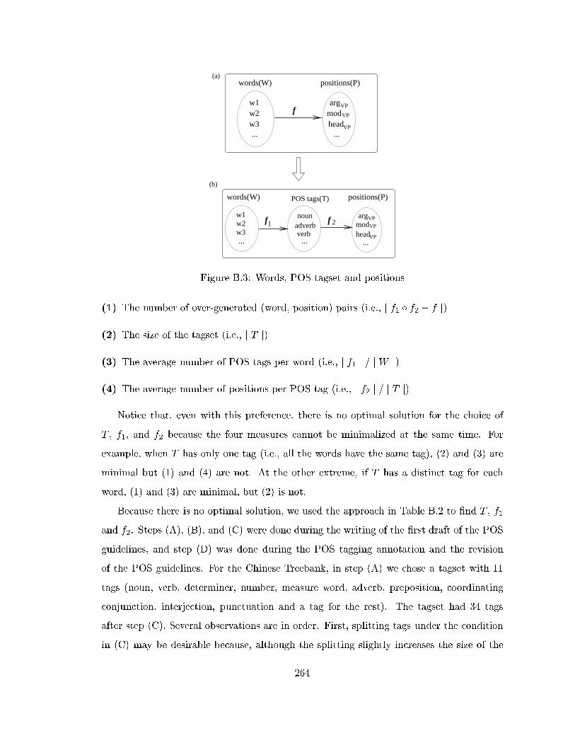
w1w2w3
adverbnoun VP
modVP
arg
headVP
POS tags(T)
w1w2w3
VP
modVP
head
arg
VP
(a)
(b)
words(W) positions(P)
words(W) positions(P)
f1 f 2
f
...
... ...
...
...verb
Figure B.3: Words, POS tagset and positions
(1) The number of over-generated (word, position) pairs (i.e., j f1 Æ f2 � f j)
(2) The size of the tagset (i.e., j T j)
(3) The average number of POS tags per word (i.e., j f1 j = jW j)
(4) The average number of positions per POS tag (i.e., j f2 j = j T j)
Notice that, even with this preference, there is no optimal solution for the choice of
T , f1, and f2 because the four measures cannot be minimalized at the same time. For
example, when T has only one tag (i.e., all the words have the same tag), (2) and (3) are
minimal but (1) and (4) are not. At the other extreme, if T has a distinct tag for each
word, (1) and (3) are minimal, but (2) is not.
Because there is no optimal solution, we used the approach in Table B.2 to �nd T , f1
and f2. Steps (A), (B), and (C) were done during the writing of the �rst draft of the POS
guidelines, and step (D) was done during the POS tagging annotation and the revision
of the POS guidelines. For the Chinese Treebank, in step (A) we chose a tagset with 11
tags (noun, verb, determiner, number, measure word, adverb, preposition, coordinating
conjunction, interjection, punctuation and a tag for the rest). The tagset had 34 tags
after step (C). Several observations are in order. First, splitting tags under the condition
in (C) may be desirable because, although the splitting slightly increases the size of the
264
tagset, it greatly reduces the number of over-generated (word, position) pairs while the
other two measures (i.e., (3) and (4)) remain roughly the same. Second, splitting the tags
in step (D-4) is much more expensive than doing it in step (C); therefore, the borderline
examples (i.e., the examples that might cause some tags to be split) should be considered
as early as possible. In an ideal situation, all the borderline examples should be considered
and the POS tagset should be �xed before the POS tagging starts, and step (D-4) should
be unnecessary. However, in practice, when guideline designers write the �rst draft of
the guidelines, they have not examined the whole Treebank; therefore, they do not know
all the possible (word, position) pairs in the Treebank (i.e., f is not completely de�ned).
As a result, they may fail to split some tags in step (C) and have to do it in step (D-4)
instead; in other words, the tagset may have to be expanded after the �rst pass of the POS
annotation starts. Fortunately, through careful design of the �rst version of the guidelines,
no such revision was needed in our project.
B.5 Syntactic bracketing guidelines
In this section, we discuss three issues on bracketing guidelines.
B.5.1 Representation scheme
The �rst issue is the choice of a representation scheme. Given that the sentences in the
corpus are very long and complex, the representation scheme needs to be robust enough
to be able to represent all the important grammatical relations and at the same time be
suÆciently simple so that the annotators can follow it easily and consistently. An overly
complicated scheme will slow down productivity and jeopardize consistency and accuracy.
At the syntactic level, we �rst need to decide what type of syntactic representation
should be used in the Treebank. Two commonly used representations are phrase struc-
tures and dependency structures. To choose between these two representations, we need to
consider many factors such as the feasibility of the conversion between them (see Chapter
7), the amount of linguistic work based on each representation, the preferences of guide-
line designers, annotators, and the potential users of the Treebank, and the availability of
265

/* Steps (A)-(C) are used to create the �rst draft of the POS tagging guidelines */(A) choose an initial tagset T , which includes only the well-established tags (such
as nouns, verbs, and adverbs) and a tag that captures the rest of tags;(B) choose f2 so that it includes only the basic positions for each tag;
(For example, nouns can be the argument of VPs and verbs can be the heads of VPs)(C) for (each tag t in T )
if (there is a position p 2 P , such that both Wt;p and Wt;p� are large)/* Wt;p is the set of words with tag t that can appear in position p *//* Wt;p� is the set of words with tag t that cannot */then consider splitting t into two tags t1 and t2 and updating f2 accordingly;
/* Step (D) is used during the POS tagging stage */(D) for (each word token w in the Treebank)
(D-1) choose a position p for the word;if (w; p) 62 fthen add (w; p) to f ;
(D-2) choose a tag t in T ;(D-3) if (w; t) 62 f1
then add (w; t) to f1;(D-4) if (t; p) 62 f2
then add (t; p) to f2;if (both Wt;p and Wt;p� are large)then consider splitting the tag t into two tags t1 and t2 andupdating f1 and f2 accordingly;
Table B.2: The process of creating and revising POS guidelines
266

annotation tools. We chose phrase structures for the Chinese Treebank for several reasons:
First, it seems that for Chinese the conversion from phrase structures to dependency struc-
tures is easier than the conversion in the opposite direction; Second, there is more Chinese
linguistic work done based on phrase structures than dependency structures; Third, most
tools available to us (such as parsers and corpus search tools, see Section B.7) are based
on phrase structures.
The next question is what information should be included in a phrase structure. We
decided to use syntactic labels, function tags, reference indexes, and empty categories. In
our representation scheme, each bracket has a syntactic label, zero or more function tags,
and zero or more reference indexes. The syntactic label indicates the syntactic category of
the phrase, whereas the function tags provide additional information such as adjunct type.
For example, when a noun phrase such as zu�o-ti�an/yesterday modi�es a verb phrase, its
syntactic label will be NP (for noun phrase) and it is given a function tag -TMP, indicating
that the NP is a temporal phrase and its function is similar to that of an adverbial phrase.
Reference indexes and a subset of empty categories (such as trace and operator) are used
to mark syntactic movement or to indicate where a phrase should be interpreted. Other
empty categories are used to mark dropped arguments, ellipsis, and so on. Our scheme is
similar to the one adopted in the Penn English Treebank (Marcus et al., 1994).
B.5.2 Syntactic constructions
The bracketing guidelines have to specify the treatment of various syntactic constructions.
Many of them (such as the ba-construction and the bei-construction) have been studied for
decades, but there is still no consensus on their treatment. To tackle this issue, we
� studied the linguistics literature,
� attended conferences on Chinese linguistics,
� had discussions with our linguistic colleagues,
� studied and tested our analyses on the relevant sentences in our corpus, and
� used special tags to mark crucial elements in these constructions.
267
For example, the word b�a in the ba-construction has been argued to be a case marker, a
secondary topic marker, a preposition, a verb, and so on in the literature. The word is
clearly di�erent from other prepositions and other verbs, and there is no strong evidence
to support the view that Chinese has overt case markers or topic markers. We believe that
the word is more likely to be a verb than a preposition, but to distinguish it from other
verbs, we assign a unique POS tag BA to it, and in the bracketing guidelines we provide
detailed instructions on how to annotate the construction. If some users of our Treebank
prefer to treat it as a preposition, our annotation can be easily converted to accommodate
that approach.
B.5.3 Ambiguities
Another issue with respect to bracketing guidelines is the treatment of ambiguous sen-
tences. In the guidelines, we classi�ed ambiguous sentences according to the cause of the
ambiguity, and speci�ed the treatment for each type. We decided to give each sentence
exactly one syntactic structure even if the sentence was ambiguous because of several
reasons. First, our Treebank is a collection of newspaper articles, rather than a list of in-
dependent sentences; as a result, very few sentences are truly ambiguous once they are put
into the context of the whole article. Second, people often don't see the ambiguity until
it is pointed out by someone else. Asking annotators to mark more than one reading of a
truly ambiguous sentence not only substantially slows down the annotation but also a�ects
the consistency of the annotation as it is almost certain that the annotators would miss
certain readings. Third, some sentences could be annotated in several ways and all these
annotations are closely related and have roughly the same meaning. For these sentences,
giving one annotation is suÆcient, and other related annotations can be derived easily if
needed. For example, some Chinese adverbs can occur either before the subject or after
it. When the subject is phonologically empty as a result of subject drop or relativization,
the empty subject (which is an empty category) can be put either before the adverb or
after the adverb with no di�erence in meaning. Consequently, the adverb either attaches
to the VP or the S, and there is no syntactic evidence to favor one annotation over the
other. If nothing is speci�ed in the guidelines and the annotator is allowed to mark the
268
empty subject in either place, inconsistency is bound to occur as either annotation can be
chosen. To eliminate this kind of inconsistency, in the guidelines we speci�ed one of the
two positions as the "default" position for the empty subject, and required annotators to
always put the empty subject in that position.
B.6 Quality control
A major challenge in providing a high-quality Treebank is ensuring consistency and ac-
curacy. Carefully documented guidelines (see Section B.2 | B.5), linguistically trained
annotators,13 and annotation supporting tools (see Section B.7) are pre-requisites to cre-
ating a high quality Treebank. In this section, we describe our strategy for quality control.
B.6.1 Two passes in each phase
As mentioned in Section B.1, the Treebank annotation was done in two phases: the �rst
phase was word segmentation and POS tagging, and the second phase was syntactic brack-
eting. At each phase, all the data were annotated at least twice with a second annotator
correcting the output of the �rst annotator. In addition to correcting human errors made
in the �rst pass, the second pass was necessary also because the guidelines had been revised
after the �rst pass (see Section B.2).
B.6.2 Double re-annotation in the bracketing phase
During the second pass of the bracketing phase, we randomly selected 20% of the Treebank
for double re-annotation. By double re-annotation, we mean that annotators re-annotate
the same �les from the output of the �rst pass. Double re-annotation allowed us to
quantitatively evaluate inter-annotator consistency and annotation accuracy. The process
of this evaluation was as follows: First, some �les from the output of the �rst pass were
13Both of our annotators are linguistics graduate students, one of whom co-authored the Bracketing
Guidelines and regularly participated in our meetings on Chinese syntax. Their knowledge of linguistics in
general, and syntax in particular, was crucial for the success of the project.
269
randomly selected and double re-annotated. Next, a software tool named evalb14 was
used to compare the two re-annotations, and any discrepancies were carefully examined
and the annotation was revised | this may in turn lead to revisions of the guidelines to
prevent a recurrence of similar inconsistencies. Then, the corrected, reconciled annotation
was considered the Gold Standard, and each of the two original re-annotations was then
run against the Gold Standard and against each other, to provide a measure of individual
annotator accuracy and inter-annotator consistency.
We �rst used this method to re-train annotators at the beginning of the second pass,15
when forty �les from the output of the �rst pass were randomly selected for double re-
annotation. After that, the annotators continued to correct �rst pass data and each week
two �les were randomly selected and double re-annotated, and the re-annotations were
compared. In this way, we continued to monitor the consistency and accuracy and to
enhance guidelines. Figure B.4 shows the accuracy of each annotator (denoted by 1st
annotator and 2nd annotator in the chart) compared to the Gold Standard and the inter-
annotator consistency during the second pass after the re-training period. The Figure
shows both measures are in the high 90% range, which is very satisfactory.16
B.6.3 Error detection using LexTract
After the second pass of the word segmentation and POS tagging phase, a list of (word,
POS tag) pairs was compiled out of the Treebank and manually checked. This process
revealed many POS tagging errors.
As discussed in Section 6.6, we also ran LexTract to build a Treebank grammar after the
second pass of bracketing phase. We then checked the grammar for implausible templates
and �xed the corresponding errors in the Treebanks.
14The software tool was written by Satoshi Sekine and Mike Collins. It takes two input �les as input
and produces precision, recall, numbers of crossing brackets, and other measures.
15The re-training process was necessary because we had revised the guidelines after the �rst pass.16Because only two �les (about 600 words) were double re-annotated and compared each week and the
complexity of sentences varied a lot from �le to �le, the consistency and accuracy rates for these �les did
not keep improving as time went by, as one might have expected.
270

80
85
90
95
100
0 2 4 6 8 10 12
(Pre
cisi
on+R
ecal
l)/2
week
1st annotator2nd annotator
agreement
Figure B.4: Accuracy and inter-annotator consistency during the second pass
B.7 The role of NLP tools
Throughout the project, we used various NLP tools to speed up and improve the quality
of the Treebank annotation.
B.7.1 Preprocessing tools
Before the �rst pass of the word segmentation and POS tagging phase, our Treebank
was automatically segmented and POS tagged by the BBN/GTE integrated stochastic
segmenter and POS tagger. The tagger was trained on the Academia Sinica Balanced
Corpus (ASBC). Because our tagset and the one used by the ASBC are quite di�erent
(Xia, 2000a), we wrote a tool to convert the ASBC tags into our tags automatically.
Although the mapping between the two tagsets was not one-to-one and the conversion
introduced new errors, this pre-processing process greatly accelerated annotation.
When the bracketing phase began, a Chinese parser was not available to us; therefore,
we started the bracketing annotation from scratch. Since the completion of our 100K-
word Treebank, two parsers have been trained on the data and their precision and recall
rates were about 80% (Bikel and Chiang, 2000). One of these parsers has been used
to pre-process the new data that we are annotating, and the pre-processing doubles the
bracketing speed (Chiou et al., 2001).
271

B.7.2 Annotation and conversion tools
To facilitate human annotation, our annotators used an interface that was created for
the English Penn Treebank (Marcus et al., 1994), which was then extended to include
word segmentation operations and other features for Chinese. The interface restricted
the combinations of keys that annotators could use, and therefore reduced the number
of careless human errors. For example, only legitimate tags (whose names appear in a
prede�ned tagset) could be entered, and the left and right brackets were added or removed
in one operation so that there were no unmatched brackets. The interface also indented
the phrase structures automatically.
In addition, we developed a collection of tools that converted the Treebank from one
format to another, as various NLP tools used slightly di�erent formats. When we revised
the guidelines after the �rst pass of each phase, some modi�cation of the Treebank was
done automatically by these conversion tools.
B.7.3 Corpus search tools
One reason that the annotation guidelines require revision is that, quite often when the
guideline designers write the draft of the guidelines, they have not checked all the relevant
data in the Treebank; as a result, they don't realize that the guidelines do not cover certain
cases until the annotators �nd these cases in the Treebank.
Corpus search tools allow the guideline designers to extract from the Treebank the
relevant sentences that match certain patterns. A search can be conducted on raw data,
segmented and POS tagged data, or bracketed data. For the �rst two types of data, sim-
ple string matching tools (such as grep in UNIX) are suÆcient. For pattern matching
on bracketed data, more sophisticated tools are needed. One of such tools (called Cor-
pusSearch) was developed by Beth Randall.17 We used this tool after the �rst pass of the
bracketing to pull out all the sentences in the Treebank that were relevant to a particular
syntactic construction, and then examined these sentences to ensure that our guidelines
could handle all these sentences correctly.
17More information about this tool can be found at http://www.cis.upenn.edu/ brandall/CSManual and
http://www.ling.upenn.edu/mideng/ppcme2dir/corpussearch.html.
272
B.7.4 Quality-control tools
As mentioned in Section B.6, we used two tools for quality control: one is the evalb, which
calculates the precision rate, recall rate, and the number of crossing brackets given two
annotations; the other is LexTract, which extracts grammars from Treebanks.
It is worth noting that both guideline preparation and Treebank annotation require
much human e�ort. While there is no doubt that using the NLP tools mentioned in this
section (such as word segmenter, POS tagger, and parser) can greatly speed up Treebank
annotation, it does not help a lot with guideline preparation because a thorough linguistic
study of the language is an irreplaceable and substantial part of guideline preparation.
B.8 Treebank guidelines and hand-crafted grammars
In many aspects, the process of making Treebank guidelines is very similar to the process
of creating a grammar by hand: both require a thorough study of the linguistics literature
and extensive discussion with linguists (see the discussion in Section B.2 { B.5); both
guidelines and hand-crafted grammars require revisions when they cannot account for
new data. Therefore, it is not surprising that the grammar extracted from a high-quality
Treebank by LexTract may look very much like a hand-crafted grammar.
On the other hand, there are two major di�erences between guidelines and hand-
crafted grammar. First, unlike hand-crafted grammars, the guidelines can use special tags
to mark a phenomenon without deciding the nature of the phenomenon. For example,
distinguishing arguments from adjuncts is notoriously diÆcult. For each dependent of a
head, the developers of a hand-crafted LTAG have to decide whether to treat the dependent
as an argument or an adjunct. In contrast, the designers of a Treebank can use function
tags to mark the function of the dependent (e.g., location, time, purpose, and so on)
without making the argument/adjunct decision, and later the users of the Treebank can
determine whether they want to treat the dependent with certain function tags as an
argument. Another example is the usage of empty categories in Treebanks and hand-
crafted grammars. To treat constructions such as NP-extraposition (see Section 6.7),
the developers of a hand-crafted LTAG have to decide whether the relation between the
273

extraposed phrase and the position where the phrase is interpreted is due to syntactic
movement. If it is due to syntactic movement, the gap and the \antecedent" should
appear in one elementary tree or one multi-component set. If it is not, this tree-locality
requirement should not be imposed. In contrast, the designers of the Treebank can use a
special empty category to mark the NP-extraposition construction without deciding the
nature of the movement.
The second di�erence between annotation guidelines and hand-crafted grammars is that
annotation guidelines have to explicitly specify the treatment for ambiguous sentences,
whereas grammars for human languages are always ambiguous and the selection of the
most likely parse for ambiguous sentences is left to the parsers that use the grammars.
B.9 Summary
We have discussed in details the approach that we used to build the Chinese Penn Tree-
bank, including the development of the guidelines for word segmentation, POS tagging
and syntactic bracketing, our methodology for quality control, and the roles of various
NLP tools. We believe that our approach is general enough to apply to monolingual text
annotation for other languages as well, and will be testing this hypothesis.
274
References
Anne Abeill�e. 1994. Syntax or Semantics? Handling Nonlocal Dependencies with MC-
TAGs or Synchronous TAGs. Computational Intelligence, 10:471{485.
Breckenridge Baldwin, Christine Doran, Je�rey Reynar, Michael Niv, B. Srinivas, and
Mark Wasson. 1997. EAGLE: An Extensible Architecture for General Linguistic En-
gineering. In Proc. of RIAO97, Montreal.
Tilman Becker, Owen Rambow, and Michael Niv. 1992. The Derivational Generative
Power, or, Scrambling is Beyond LCFRS. Technical Report IRCS-92-38, University of
Pennsylvania.
Tilman Becker. 1994. Patterns in Metarules. In Proc. of the 3rd International Workshop
on TAG and Related Frameworks (TAG+3), Paris, France.
Ann Bies, Mark Ferguson, Karen Katz, and Robert MacIntyre. 1995. Bracketing Guide-
lines for Treebank II Style Penn Treebank Project.
Daniel M. Bikel and David Chiang. 2000. Two Statistical Parsing Models Applied to the
Chinese Treebank. In Proc. of the 2nd Chinese Language Processing Workshop, Hong
Kong, China.
E. Black, S. Abney, D. Flickinger, C. Gdaniec, and et. al. 1991. A Procedure for Quantita-
tively Comparing the Syntactic Coverage of English grammars. In Proc. of the DARPA
Speech and Natural Language Workshop.
Tonia Bleam. 1994. Clitic Climbing in TAG: A GB Perspective. In Proc. of 3rd Interna-
tional Workshop on TAG and Related Frameworks (TAG+3).
J. Bresnan, R. Kaplan, S. Peters, and A. Zaenen. 1982. Cross-Serial Dependencies in
Dutch. Linguistic Inquiry.
Marie-Helene Candito. 1996. A Principle-Based Hierarchical Representation of LTAGs.
In Proc. of COLING-1996, Copenhagen, Denmark.
275

R. Chandrasekar and B. Srinivas. 1997. Gleaning information from the Web: Using Syntax
to Filter out Irrelevant Information. In Proc. of AAAI 1997 Spring Symposium on NLP
on the World Wide Web.
Eugene Charniak. 1997. Statistical Parsing with a Context-Free Grammar and Word
Statistics. In Proc. of AAAI-1997.
John Chen and K. Vijay-Shanker. 2000. Automated Extraction of TAGs from the Penn
Treebank. In Proc. of the 6th International Workshop on Parsing Technologies (IWPT-
2000), Italy.
John Chen, Srinivas Bangalore, and K. Vijay-Shanker. 1999. New Models for Improving
Supertag Disambiguation. In Proc. of EACL-1999.
David Chiang. 2000. Statistical Parsing with an Automatically-Extracted Tree Adjoining
Grammar. In Proc. of ACL-2000.
Chinese Knowledge Information Processing Group. 1996. Shouwen Jiezi - A study of
Chinese Word Boundaries and Segmentation Standard for Information Processing (in
Chinese). Technical report, Taipei: Academia Sinica.
Fu-Dong Chiou, David Chiang, and Martha Palmer. 2001. Facilitating Treebank Annotat-
ing Using a Statistical Parser. In Proc. of the Human Language Technology Conference
(HLT-2001), San Diego, CA.
Michael Collins, Jan Haji�c, Lance Ramshaw, and Christoph Tillmann. 1999. A Statistical
Parser for Czech. In Proc. of ACL-1999, pages 505{512.
Mike Collins. 1997. Three Generative, Lexicalised Models for Statistical Parsing. In Proc.
of ACL-1997.
Bernard Comrie. 1987. The World's Major Languages. Oxford University Press, New
York.
Thomas Cormen, Charles Leiserson, and Ronald Rivest. 1990. Introduction to Algorithms.
The MIT Press.
276

Michael Covington. 1994a. An Empirically Motivated Reinterpretation of Dependency
Grammar. Research Report AI-1994-01.
Michael Covington. 1994b. GB Theory as Dependency Grammar. Research Report AI-
1992-03.
Christy Doran, Beth Ann Hockey, Anoop Sarkar, Bangalore Srinivas, and Fei Xia. 2000.
Evolution of the XTAG System. In Anne Abeill�e and Owen Rambow, editors, Tree
Adjoining Grammar: Formalism, Computation, Applications. CSLI Publications.
Christine Doran. 1998. Incorporating Punctuation into the Sentence Grammar: A Lexi-
calized Tree Adjoining Grammar Perspective. Ph.D. thesis, University of Pennsylvania.
Christine Doran. 2000. Punctuation in a Lexicalized Grammar. In Proc. of 5th Interna-
tional Workshop on TAG and Related Frameworks (TAG+5).
B. J. Dorr. 1993. Machine Translation: a View from the Lexicon. MIT Press, Boston,
Mass.
Roger Evans and Gerald Gazdar. 1989. Inference in DATR. In Proc. of EACL-1989.
Roger Evans, Gerald Gazdar, and David Weir. 1995. Encoding Lexicalized Tree Adjoin-
ing Grammars with a Nonmonotonic Inheritance Hierarchy. In Proc. of ACL-1995,
Cambridge, MA.
Shengli Feng. 1998. Short Passives in Modern and Classical Chinese. In The 1998 Yearbook
of the Linguistic Association of Finland (41-68).
Haim Gaifman. 1965. Dependency Systems and Phrase-Structure Systems. Information
and Control, pages 304{337.
Qianyan Gong. 1997. Zhongguo Yufaxue Shi (The History of Chinese Syntax). Yuwen
Press.
J. Goodman. 1997. Probabilistic Feature Grammars. In Proc. of the International Work-
shop on Parsing Technologies.
277
XTAG Research Group. 2001. A lexicalized tree adjoining grammar for english. Technical
Report IRCS 01-03, University of Pennsylvania.
Jan Haji�c. 1998. Building a Syntactically Annotated Corpus: The Prague Dependency
Treebank. Issues of Valency and Meaning (Festschrift for Jarmila Panevov�a).
Chunghye Han and Na-Rae Han. 2001. Part-of-Speech Tagging Guidelines for the Penn
Korean Treebank (forthcoming).
Chunghye Han, Na-Rae Han, and Eon-Suk Ko. 2001. Bracketing Guidelines for the Penn
Korean Treebank (forthcoming).
Caroline Heycock. 1987. The Structure of the Japanese Causative. University of Pennsyl-
vania.
J. Higginbotham. 1984. English Is Not a Context-Free Language. Linguistic Inquiry.
Aravind Joshi and Yves Schabes. 1997. Tree Adjoining Grammars. In A. Salomma and
G. Rosenberg, editors, Handbook of Formal Languages and Automata. Springer-Verlag,
Herdelberg.
Aravind Joshi and B. Srinivas. 1994. Disambiguation of Super Parts of Speech (or Su-
pertags): Almost Parsing. In Proc. of COLING-1994.
Aravind Joshi and K. Vijay-Shanker. 1999. Compositional Semantics with LTAG: How
Much Underspeci�cation Is Necessary? In Proc. of 3nd International Workshop on
Computational Semantics.
Aravind K. Joshi, L. Levy, and M. Takahashi. 1975. Tree Adjunct Grammars. Journal of
Computer and System Sciences.
Aravind K. Joshi. 1985. Tree Adjoining Grammars: How Much Context Sensitivity Is Re-
quired to Provide a Reasonable Structural Description. In D. Dowty, I. Karttunen, and
A. Zwicky, editors, Natural Language Parsing, pages 206{250. Cambridge University
Press, Cambridge, U.K.
278
Aravind K. Joshi. 1987. An Introduction to Tree Adjoining Grammars. In Alexis
Manaster-Ramer, editor, Mathematics of Language. John Bebjamins Publishing Co,
Amsterdam/Philadelphia.
Laura Kallmeyer and Aravind Joshi. 1999. Underspeci�ed Semantics with LTAG.
R. Kasper, B. Kiefer, K. Netter, and K. Vijay-Shanker. 1995. Compiling HPSG into TAG.
In Proc. of ACL-1995.
Karin Kipper, Hoa Trang Dang, and Martha Palmer. 2000. Class-based Construction of
a Verb Lexicon. In Proc. of AAAI-2000.
Anthony S. Kroch and Aravind K. Joshi. 1985. The Linguistic Relevance of Tree Ad-
joining Grammars. Technical Report MS-CIS-85-16, Department of Computer and
Information Science, University of Pennsylvania.
Anthony S. Kroch. 1989. Asymmetries in Long Distance Extraction in a TAG Gram-
mar. In M. Baltin and A. Kroch, editors, Alternative Conceptions of Phrase Structure.
University of Chicago Press.
Alexander Krotov, Mark Hepple, Robert Gaizauskas, and Yorick Wilks. 1998. Compacting
the Penn Treebank Grammar. In Proc. of ACL-1998.
Seth Kulick. 1998. TAG and Clitic Climbing in Romance. In Proc. of 4th International
Workshop on TAG and Related Frameworks (TAG+4).
Seth Kulick. 2000. Constraining Non-Local Dependencies in Tree Adjoining Grammar:
Computational and Linguistic Perspectives. Ph.D. thesis, University of Pennsylvania.
Beth Levin. 1993. English Verb Classes and Alternations: A Preliminary Investigation.
The University of Chicago Press.
Y. Liu, Q. Tan, and X. Shen. 1993. Segmentation Standard for Modern Chinese Informa-
tion Processing and Automatic Segmentation Methodology.
David M. Magerman. 1995. Statistical Decision-Tree Models for Parsing. In Proc. of
ACL-1995.
279
Benoit Mandelbrot. 1954. Structure formelle des textes et communication. Word, 10.
Christopher D. Manning and Hinrich Sch�utze. 1999. Foundations of Statistical Natural
Language Processing. The MIT Press.
M. Marcus, B. Santorini, and M. A. Marcinkiewicz. 1993. Building a Large Annotated
Corpus of English: the Penn Treebank. Computational Linguistics.
Mitchell Marcus, Grace Kim, Mary Ann Marcinkiewicz, et al. 1994. The Penn Treebank:
Annotating Predicate Argument Structure. In Proc of ARPA speech and Natural lan-
guage workshop.
K. F. McCoy, K. Vijay-Shanker, and G. Yang. 1992. A Functional Approach to Generation
with TAG. In Proc. of ACL-1992.
Dan Melamed. 1999. Bitext maps and alignment via pattern recognition. Computational
Linguistics.
Gunter Neumann. 1998. Automatic Extraction of Stochastic Lexicalized Tree Grammars
from Treebanks. In Proc. of the 4th International Workshop on TAG and Related
Frameworks (TAG+4).
Jerome L. Packard, editor. 1998. New Approaches to Chinese Word Formation: Morphol-
ogy, Phonology and the Lexicon in Modern and Ancient Chinese. Berlin ; New York :
Mouton de Gruyter.
Jerome L. Packard. 2000. The Morphology of Chinese: A linguistic and Cognitive Ap-
proach. Cambridge University Press.
Martha Palmer, Owen Rambow, and Alexis Nasr. 1998. Rapid Prototyping of Domain-
Speci�c Machine Translation System. In Proc. of AMTA-1998, Langhorne, PA.
Martha Palmer, Joseph Rosenzweig, and William Schuler. 1999. Capturing motion verb
generalizations with synchronous tag. In Patrick St. Dizier, editor, Predicative Forms
in NLP: Text, Speech and Language Technology Series, pages 229{256. Kluwer Press,
Dordrecht, The Netherlands.
280
Rashmi Prasad and Anoop Sarkar. 2000. Comparing Test-Suite Based Evaluation and
Corpus-Based Evaluation of a Wide-Coverage Grammar for English. In Proc. of LREC
satellite workshop Using Evaluation within HLT Programs: Results and Trends, Athen,
Greece.
Owen Rambow and Aravind K. Joshi. 1997. A Formal Look at Dependency Grammars
and Phrase Structure Grammars with Special Consideration of Word-Order Phenom-
ena. In L. Wenner, editor, Recent Trends in Meaning-Text Theory. John Benjamin,
Amsterdam, Philadelphia.
Adwait Ratnaparkhi. 1998. Maximum Entropy Models for Natural Language Ambiguity
Resolution. Ph.D. thesis, University of Pennsylvania.
James Rogers and K. Vijay-Shanker. 1994. Obtaining Trees from Their Descriptions: An
Application to Tree Adjoining Grammars. Computational Intelligence, 10(4).
Beatrice Santorini. 1990. Part-of-Speech Tagging Guidelines for the Penn Treebank
Project. Technical report, Department of Computer and Information Science, Uni-
versity of Pennsylvania.
Anoop Sarkar and Aravind Joshi. 1996. Coordination in Tree Adjoining Grammars:
Formalization and Implementation. In Proc. of COLING-1996, Copenhagen, Denmark.
Anoop Sarkar. 2001. Applying Co-Training Methods to Statistical Parsing. In Proc. of
NAACL-2001.
The XTAG-Group. 1998. A Lexicalized Tree Adjoining Grammar for English. Technical
Report IRCS 98-18, University of Pennsylvania.
Yves Schabes and Stuart Shieber. 1992. An Alternative Conception of Tree-Adjoining
Derivation. In Proc. of ACL-1992.
Yves Schabes and Richard Waters. 1995. Tree insertion grammar: a cubic-time parsable
formalism that lexicalizes context-free grammar without changing the trees produced.
Computational Linguistics.
281

Yves Schabes. 1990. Mathematical and Computational Aspects of Lexicalized Grammars.
Ph.D. thesis, University of Pennsylvania.
Anna Maria Di Sciullo and Edwin Williams. 1987. On the De�nition of Word. The MIT
Press.
Masayoshi Shibatani, editor. 1976. The Grammar of causative constructions. New York:
Academic Press.
S. Shieber. 1984. Evidence Against the Context-Freeness of Natural Language. SRI
International Technical Note no. 330.
W. Skut, B. Krenn, T. Brants, and H. Uszkoreit. 1997. An Annotation Scheme for Free
Word Order Languages. In Proc. of 5th International Conference of Applied Natural
Language.
R. Sproat, W. Gale, C. Shih, and N. Chang. 1996. A Stochastic Finite-state Word
Segmentation Algorithm for Chinese. Computational Linguistics.
B. Srinivas, Anoop Sarkar, Christine Doran, and Beth Ann Hockey. 1998. Grammar and
Parser Evaluation in the XTAG Project. In Proc. of the Workshop on Evaluation of
Parsing Systems, Granada, Spain.
B. Srinivas. 1997. Complexity of Lexical Descriptions and Its Relevance to Partial Parsing.
Ph.D. thesis, University of Pennsylvania.
Matthew Stone and Christine Doran. 1997. Sentence Planning as Description Using Tree
Adjoining Grammar. In Proc. of ACL-1997.
K. Vijay-Shanker and Yves Schabes. 1992. Structure Sharing in Lexicalized Tree Adjoining
Grammar. In Proc. of COLING-1992, Nantes, France.
K. Vijay-Shanker. 1987. A Study of Tree Adjoining Grammars. Ph.D. thesis, Department
of Computer and Information Science, University of Pennsylvania.
282
Bonnie Webber and Aravind Joshi. 1998. Anchoring a Lexicalized Tree Adjoining Gram-
mar for Discourse. In Proc. of ACL-COLING Workshop on Discourse Relations and
Discourse Markers.
Bonnie Webber, Alistair Knott, Matthew Stone, and Aravind Joshi. 1999. What Are
Little Trees Made of: A Structural and Presuppositional Account Using Lexicalized
TAG. In Proc. of International Workshop on Levels of Representation in Discourse
(LORID-1999).
D. Weir. 1988. Characterizing Mildly Context-Sensitive Grammar Formalisms. Ph.D.
thesis, University of Pennsylvania.
Fei Xia and Tonia Bleam. 2000. A Corpus-Based Evaluation of Syntactic Locality in TAGs.
In Proc. of 5th International Workshop on TAG and Related Frameworks (TAG+5).
Fei Xia and Martha Palmer. 2000. Evaluating the Coverage of LTAGs on Annotated
Corpora. In Proc. of LREC satellite workshop Using Evaluation within HLT Programs:
Results and Trends.
Fei Xia, Martha Palmer, K. Vijay-shanker, and Joseph Rosenzweig. 1998. Consistent
Grammar Development Using Partial-tree Descriptions for Lexicalized Tree-Adjoining
Grammar. In Proc. of tag+4.
Fei Xia, Martha Palmer, and K. Vijay-Shanker. 1999. Toward Semi-Automating Grammar
Development. In Proc. of 5th Natural Language Processing Paci�c Rim Symposium
(NLPRS-1999), Beijing, China.
Fei Xia, Martha Palmer, and Aravind Joshi. 2000a. A Uniform Method of Grammar
Extraction and its Applications. In Proc. of Joint SIGDAT Conference on Empirical
Methods in Natural Language Processing and Very Large Corpora (EMNLP-2000).
Fei Xia, Martha Palmer, Nianwen Xue, Mary Ellen Okurowski, John Kovarik, Shizhe
Huang, Tony Kroch, and Mitch Marcus. 2000b. Developing Guidelines and Ensuring
Consistency for Chinese Text Annotation. In Proc. of the 2nd International Conference
on Language Resources and Evaluation (LREC-2000), Athens, Greece.
283

Fei Xia, Chunghye Han, Martha Palmer, and Aravind Joshi. 2001. Automatically Ex-
tracting and Comparing Lexicalized Grammars for Di�erent Languages. In Proc. of
the Seventeenth International Joint Conference on Arti�cial Intelligence (IJCAI-2001),
Seattle, Washington.
Fei Xia. 2000a. The Part-of-Speech Guidelines for Chinese Treebank Project. Technical
Report IRCS 00-07, University of Pennsylvania.
Fei Xia. 2000b. The Segmentation Guidelines for Chinese Treebank Project. Technical
Report IRCS 00-06, University of Pennsylvania.
Nianwen Xue and Fei Xia. 2000. The Bracketing Guidelines for Chinese Treebank Project.
Technical Report IRCS 00-08, University of Pennsylvania.
George Kingsley Zipf. 1949. Human Behavior and the Principle of Least E�ort. Hafner
Publishing Company.
284