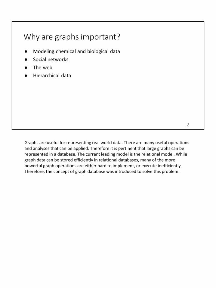
Graphs are useful for representing real world data. There are many useful operations and analyses that can be applied. Therefore it is pertinent that large graphs can be represented in a database. The current leading model is the relational model. While graph data can be stored efficiently in relational databases, many of the more powerful graph operations are either hard to implement, or execute inefficiently. Therefore, the concept of graph database was introduced to solve this problem.

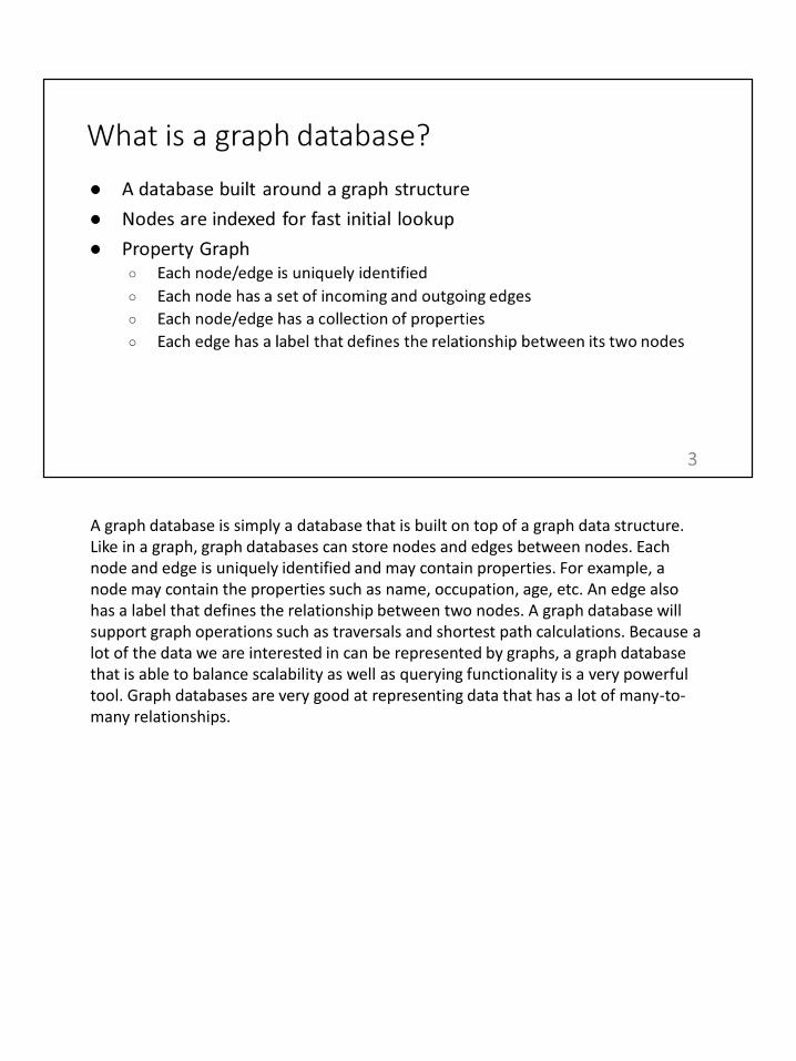
A graph database is simply a database that is built on top of a graph data structure. Like in a graph, graph databases can store nodes and edges between nodes. Each node and edge is uniquely identified and may contain properties. For example, a node may contain the properties such as name, occupation, age, etc. An edge also has a label that defines the relationship between two nodes. A graph database will support graph operations such as traversals and shortest path calculations. Because a lot of the data we are interested in can be represented by graphs, a graph database that is able to balance scalability as well as querying functionality is a very powerful tool. Graph databases are very good at representing data that has a lot of many-to-many relationships.

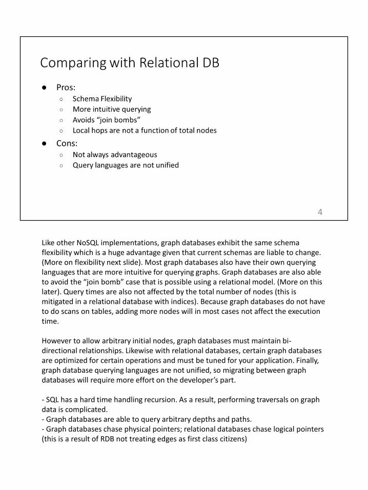
Like other NoSQL implementations, graph databases exhibit the same schema flexibility which is a huge advantage given that current schemas are liable to change. (More on flexibility next slide). Most graph databases also have their own querying languages that are more intuitive for querying graphs. Graph databases are also able to avoid the “join bomb” case that is possible using a relational model. (More on this later). Query times are also not affected by the total number of nodes (this is mitigated in a relational database with indices). Because graph databases do not have to do scans on tables, adding more nodes will in most cases not affect the execution time.

However to allow arbitrary initial nodes, graph databases must maintain bi-directional relationships. Likewise with relational databases, certain graph databases are optimized for certain operations and must be tuned for your application. Finally, graph database querying languages are not unified, so migrating between graph databases will require more effort on the developer’s part.

- SQL has a hard time handling recursion. As a result, performing traversals on graph data is complicated. - Graph databases are able to query arbitrary depths and paths.- Graph databases chase physical pointers; relational databases chase logical pointers (this is a result of RDB not treating edges as first class citizens)

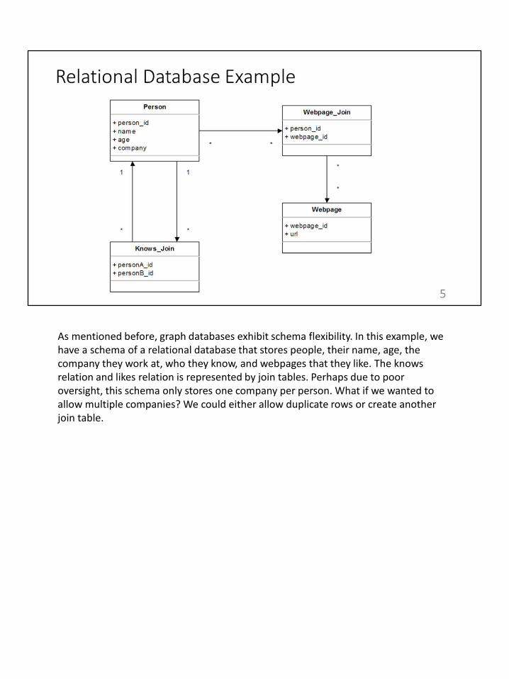
As mentioned before, graph databases exhibit schema flexibility. In this example, we have a schema of a relational database that stores people, their name, age, the company they work at, who they know, and webpages that they like. The knows relation and likes relation is represented by join tables. Perhaps due to poor oversight, this schema only stores one company per person. What if we wanted to allow multiple companies? We could either allow duplicate rows or create another join table.

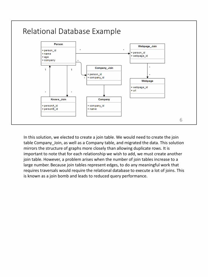
In this solution, we elected to create a join table. We would need to create the join table Company_Join, as well as a Company table, and migrated the data. This solution mirrors the structure of graphs more closely than allowing duplicate rows. It is important to note that for each relationship we wish to add, we must create another join table. However, a problem arises when the number of join tables increase to a large number. Because join tables represent edges, to do any meaningful work that requires traversals would require the relational database to execute a lot of joins. This is known as a join bomb and leads to reduced query performance.

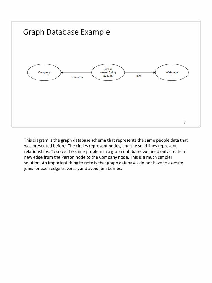
This diagram is the graph database schema that represents the same people data that was presented before. The circles represent nodes, and the solid lines represent relationships. To solve the same problem in a graph database, we need only create a new edge from the Person node to the Company node. This is a much simpler solution. An important thing to note is that graph databases do not have to execute joins for each edge traversal, and avoid join bombs.

8

There are several questions you might want to ask of data stored in a graph. List for me all the nodes or edges that have a certain property. Find subgraphs that match a given set of relationships. Further, figuring out if two nodes can reach each other (with a limit of hops, even) is easy to think of in a graph model.

9

How do we translate these questions into actionable queries? Let’s use the popular Neo4j graph database as an example. You can query Neo4j using it’s SQL-like query language Cypher. There is no one query language for graph databases.

10

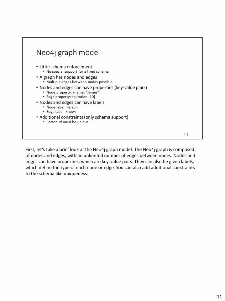
First, let’s take a brief look at the Neo4j graph model. The Neo4j graph is composed of nodes and edges, with an unlimited number of edges between nodes. Nodes and edges can have properties, which are key-value pairs. They can also be given labels, which define the type of each node or edge. You can also add additional constraints to the schema like uniqueness.

11

12

As I’ve said, we’ll be using a SQL-like language called Cypher to query a Neo4j database. You can do all of the usual sorts of operations using Cypher – retrievals, adding, updating, and deleting data. You can also manage the database itself by adding indexes and constraints.

13

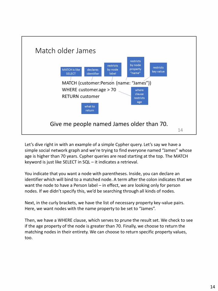
Let’s dive right in with an example of a simple Cypher query. Let’s say we have a simple social network graph and we’re trying to find everyone named “James” whose age is higher than 70 years. Cypher queries are read starting at the top. The MATCH keyword is just like SELECT in SQL – it indicates a retrieval.

You indicate that you want a node with parentheses. Inside, you can declare an identifier which will bind to a matched node. A term after the colon indicates that we want the node to have a Person label – in effect, we are looking only for person nodes. If we didn’t specify this, we’d be searching through all kinds of nodes.

Next, in the curly brackets, we have the list of necessary property key-value pairs. Here, we want nodes with the name property to be set to “James”.

Then, we have a WHERE clause, which serves to prune the result set. We check to see if the age property of the node is greater than 70. Finally, we choose to return the matching nodes in their entirety. We can choose to return specific property values, too.

14

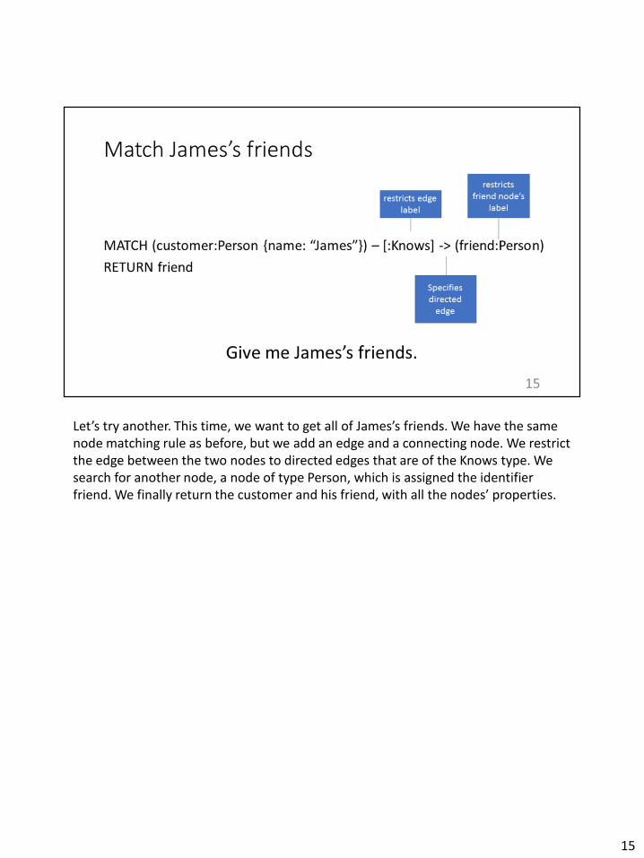
Let’s try another. This time, we want to get all of James’s friends. We have the same node matching rule as before, but we add an edge and a connecting node. We restrict the edge between the two nodes to directed edges that are of the Knows type. We search for another node, a node of type Person, which is assigned the identifier friend. We finally return the customer and his friend, with all the nodes’ properties.

15

We can make a simple modification to get friends that are two hops away (friends of friends.) We can see from the return statement that we’ll be returning matched Person nodes.

16

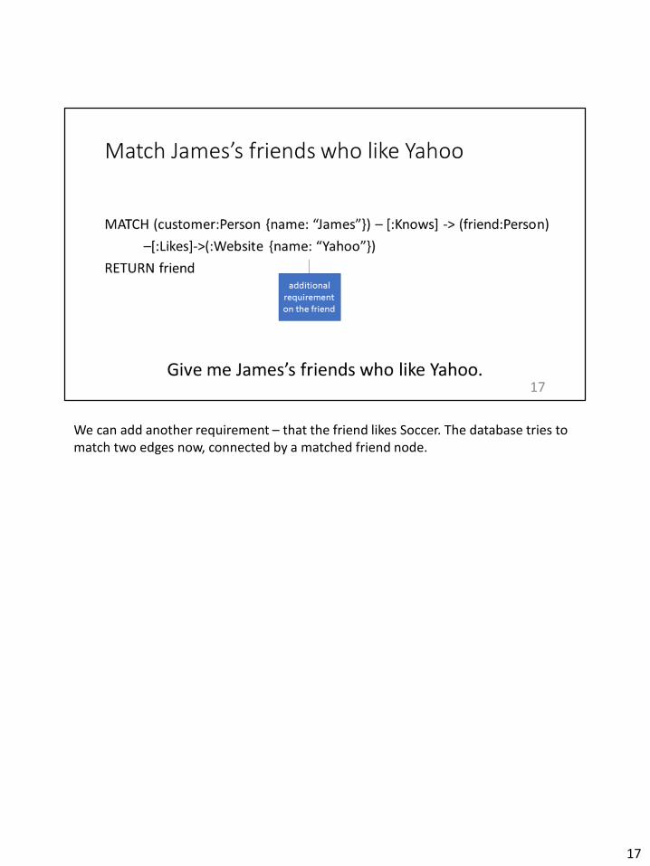
We can add another requirement – that the friend likes Soccer. The database tries to match two edges now, connected by a matched friend node.

17

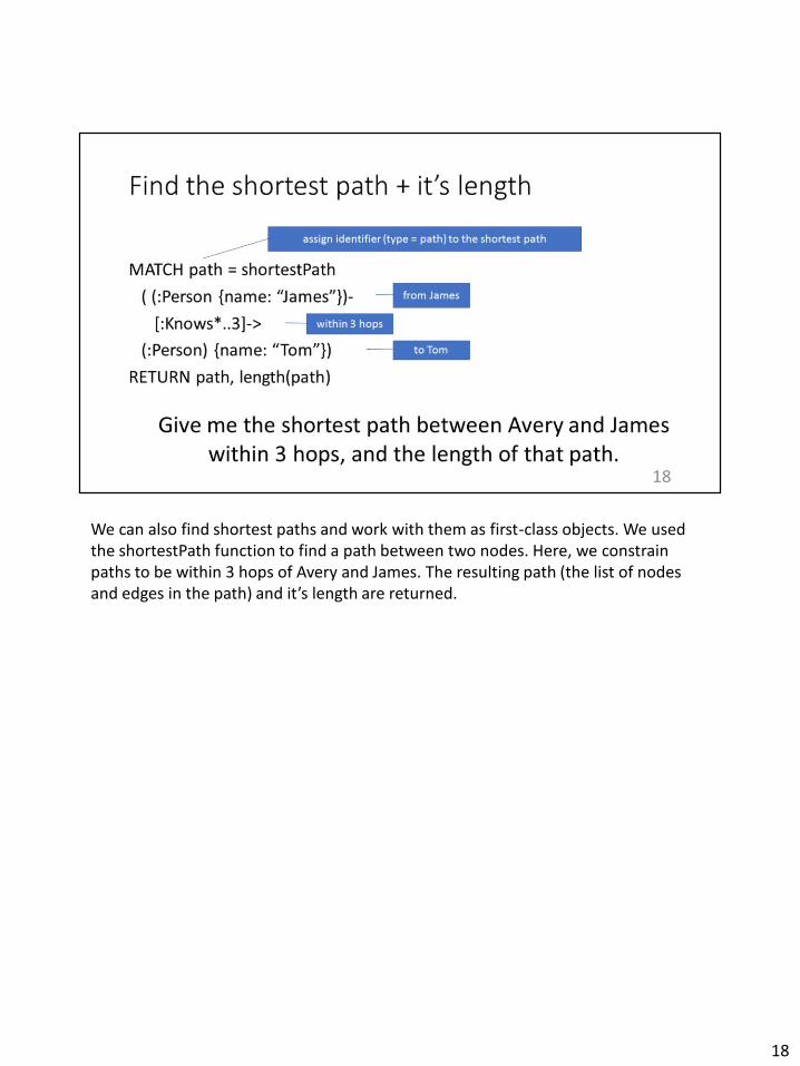
We can also find shortest paths and work with them as first-class objects. We used the shortestPath function to find a path between two nodes. Here, we constrain paths to be within 3 hops of Avery and James. The resulting path (the list of nodes and edges in the path) and it’s length are returned.

18

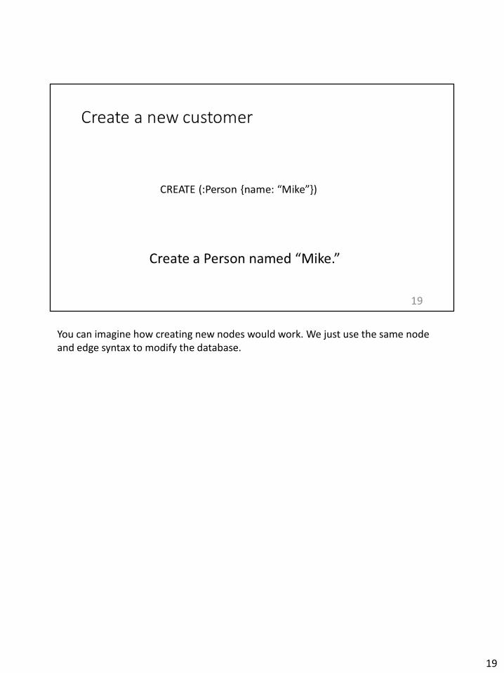
You can imagine how creating new nodes would work. We just use the same node and edge syntax to modify the database.

19

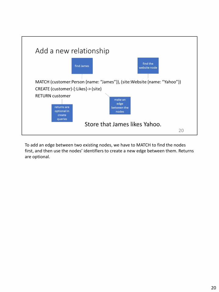
To add an edge between two existing nodes, we have to MATCH to find the nodes first, and then use the nodes’ identifiers to create a new edge between them. Returns are optional.

20

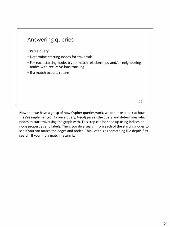
Now that we have a grasp of how Cypher queries work, we can take a look at how they’re implemented. To run a query, Neo4j parses the query and determines which nodes to start traversing the graph with. This step can be sped up using indices on node properties and labels. Then, you do a search from each of the starting nodes to see if you can match the edges and nodes. Think of this as something like depth-first search. If you find a match, return it.

21

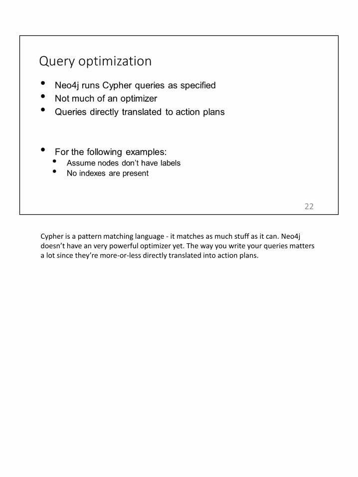
Cypher is a pattern matching language - it matches as much stuff as it can. Neo4jdoesn’t have an very powerful optimizer yet. The way you write your queries matters a lot since they’re more-or-less directly translated into action plans.

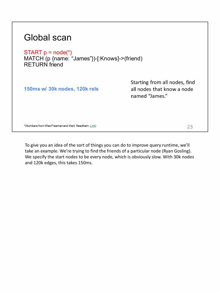
To give you an idea of the sort of things you can do to improve query runtime, we’ll take an example. We’re trying to find the friends of a particular node (Ryan Gosling). We specify the start nodes to be every node, which is obviously slow. With 30k nodes and 120k edges, this takes 150ms.

Now, let’s add a Person label to Ryan, so we can find him faster.

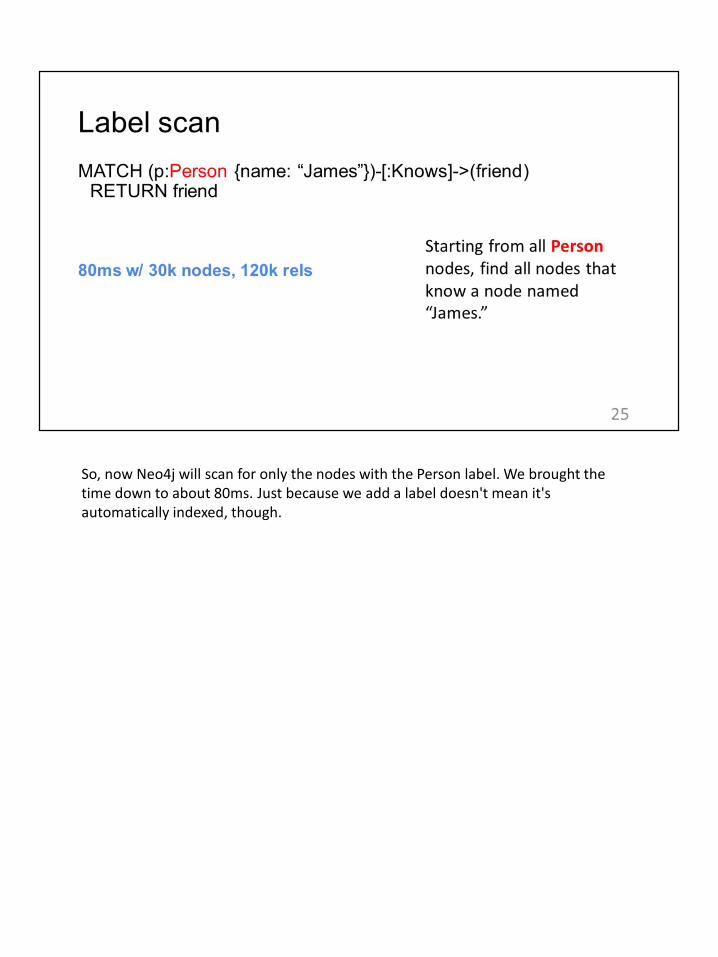
So, now Neo4j will scan for only the nodes with the Person label. We brought the time down to about 80ms. Just because we add a label doesn't mean it's automatically indexed, though.

We need to explicitly add indexes on the properties that you're likely to query against. Here, we do it for the name properties of label nodes.

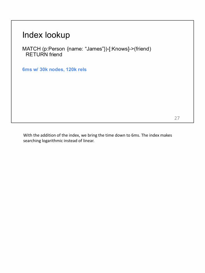
With the addition of the index, we bring the time down to 6ms. The index makes searching logarithmic instead of linear.

The main take-away is that the way your write your query has a big impact on it’s performance. Make sure to use labels, indices, and be careful about things like predicate order.

28

The motivation for this part of the presentation is to compare Graph DBs with relational DBs from a social networking application point of view. Why? This is mainly to justify the huge spurt in the adoption of graph DBs that has been seen in such applications though they are also being adopted in sectors like HR, Finance, etc The benchmarks proposed are from an academic point of view, focusing on query times (seconds) rather than cost ($) but nevertheless are important microbenchmarks showing exactly where graph DBs perform better than relational DBs rather than simply saying that graph DBs are better for all graph related queries. Also, albeit this is less important, it gives a general idea about how one should go about comparing two frameworks / systems.

30

There have been initiatives likes LDBC and LinkBench (based off of Facebook), however, they measure ops like: load time or complete graph traversal, without focussing on a specific application like social networks and the wide range of queries that manifest in such a scenario. Also they are more industry-oriented benchmarks whereas this serves to be more academic. More details on next slide..

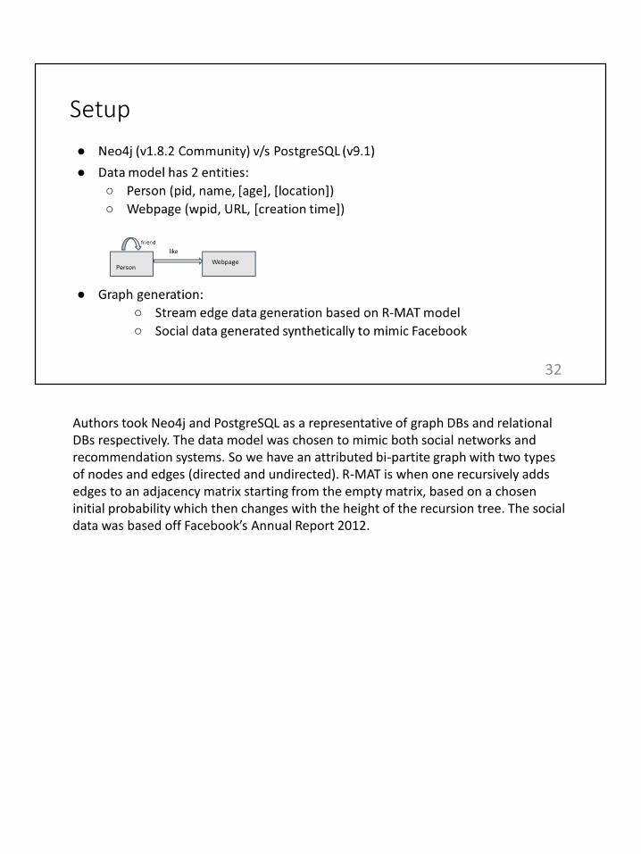
Authors took Neo4j and PostgreSQL as a representative of graph DBs and relational DBs respectively. The data model was chosen to mimic both social networks and recommendation systems. So we have an attributed bi-partite graph with two types of nodes and edges (directed and undirected). R-MAT is when one recursively adds edges to an adjacency matrix starting from the empty matrix, based on a chosen initial probability which then changes with the height of the recursion tree. The social data was based off Facebook’s Annual Report 2012.

These are the list of primitive queries that span 5 major query types: select, adjacency, reachability, pattern matching and summarization. Most of the queries, if not all, over social networks / recommendation systems are composed of a few of these primitive queries, hence these were considered an essential component of the benchmark.

The test data was an XML file which contained data to be used in the creation of query instances. The performance metrics are standard and since this is an academic benchmark they did not include metrics like price per transaction, etcNext slide goes into more detail about how many instances, the setup, etc

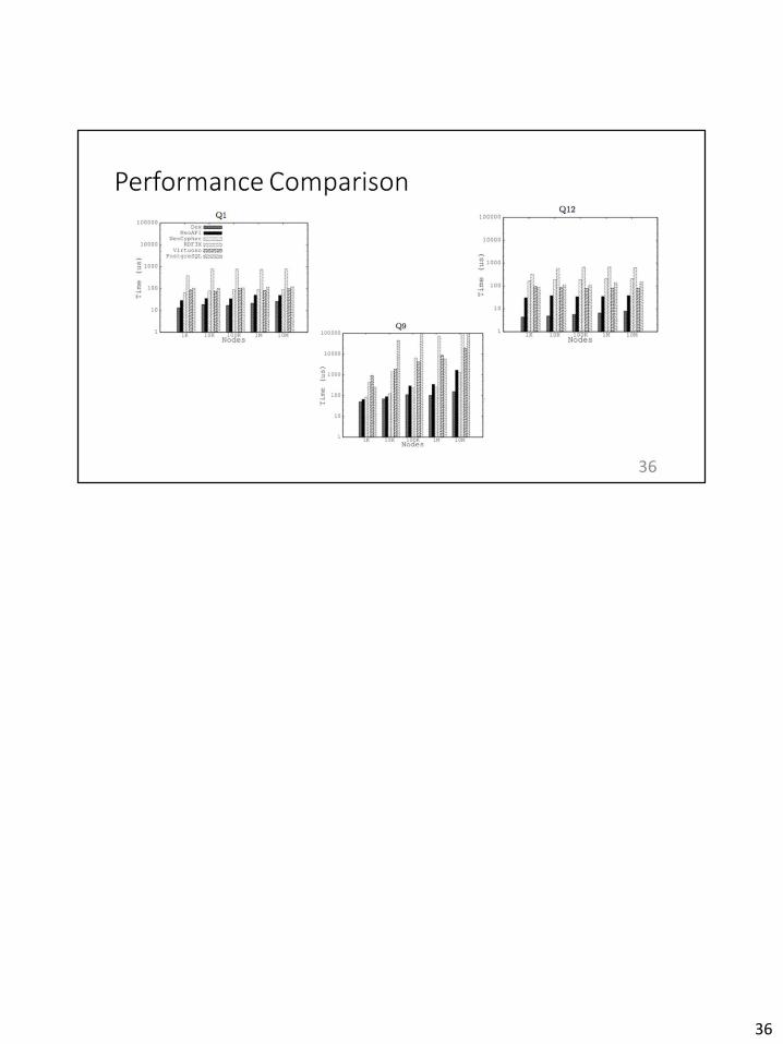
Representative queries were chosen from each of the 5 categories. The machine is a standard high-end desktop system (2012)

36

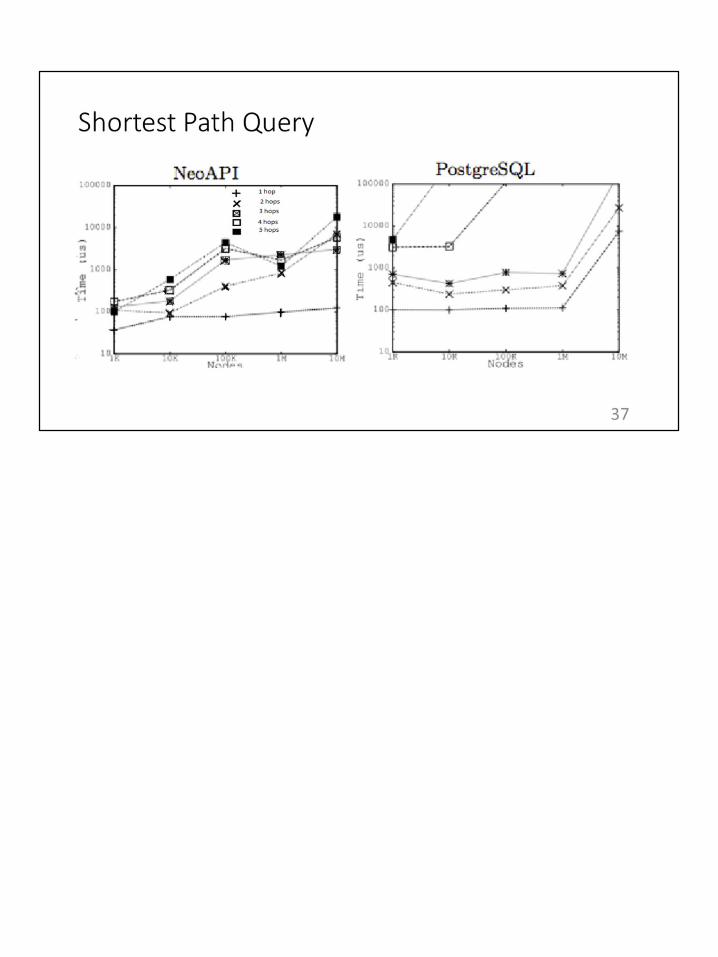
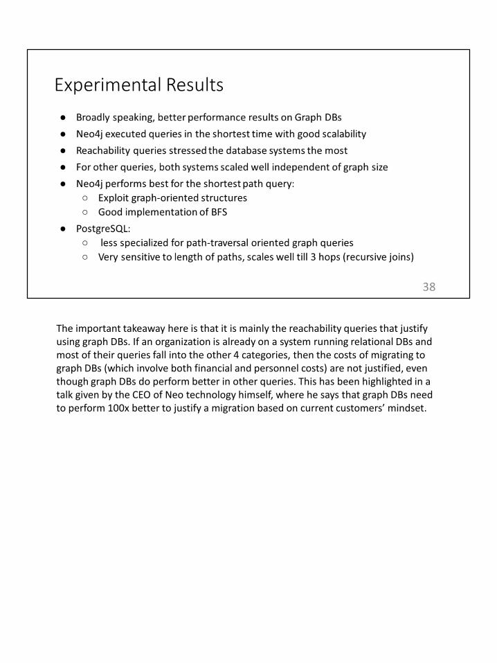
The important takeaway here is that it is mainly the reachability queries that justify using graph DBs. If an organization is already on a system running relational DBs and most of their queries fall into the other 4 categories, then the costs of migrating to graph DBs (which involve both financial and personnel costs) are not justified, even though graph DBs do perform better in other queries. This has been highlighted in a talk given by the CEO of Neo technology himself, where he says that graph DBs need to perform 100x better to justify a migration based on current customers’ mindset.

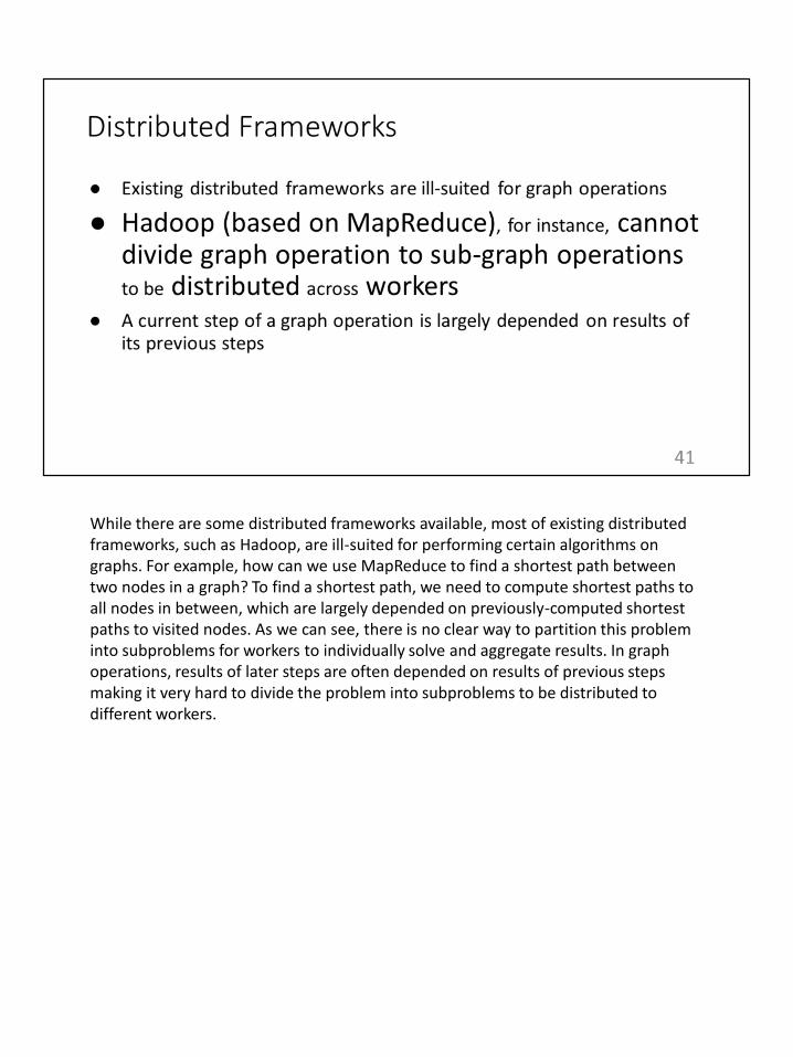
While there are some distributed frameworks available, most of existing distributed frameworks, such as Hadoop, are ill-suited for performing certain algorithms on graphs. For example, how can we use MapReduce to find a shortest path between two nodes in a graph? To find a shortest path, we need to compute shortest paths to all nodes in between, which are largely depended on previously-computed shortest paths to visited nodes. As we can see, there is no clear way to partition this problem into subproblems for workers to individually solve and aggregate results. In graph operations, results of later steps are often depended on results of previous steps making it very hard to divide the problem into subproblems to be distributed to different workers.

To address the issue, Google developed what is called Pregel to allow the execution of arbitrary graph algorithms on graphs in distributed ways. Pregel is easily scalable by adding more Pregel instances, or workers, and it ensures fault tolerance via the use of Master and Worker pings and saved states. It takes a graph as an input, and outputs either a set of vertices, an aggregated value, or an isomorphic graph based on the query.

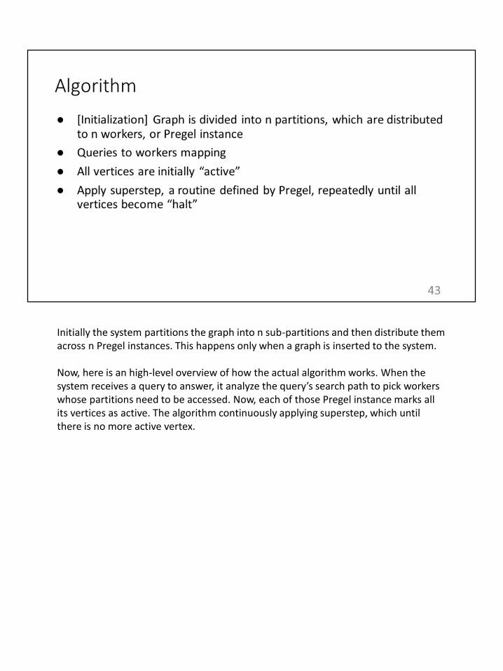
Initially the system partitions the graph into n sub-partitions and then distribute them across n Pregel instances. This happens only when a graph is inserted to the system.

Now, here is an high-level overview of how the actual algorithm works. When the system receives a query to answer, it analyze the query’s search path to pick workers whose partitions need to be accessed. Now, each of those Pregel instance marks all its vertices as active. The algorithm continuously applying superstep, which until there is no more active vertex.

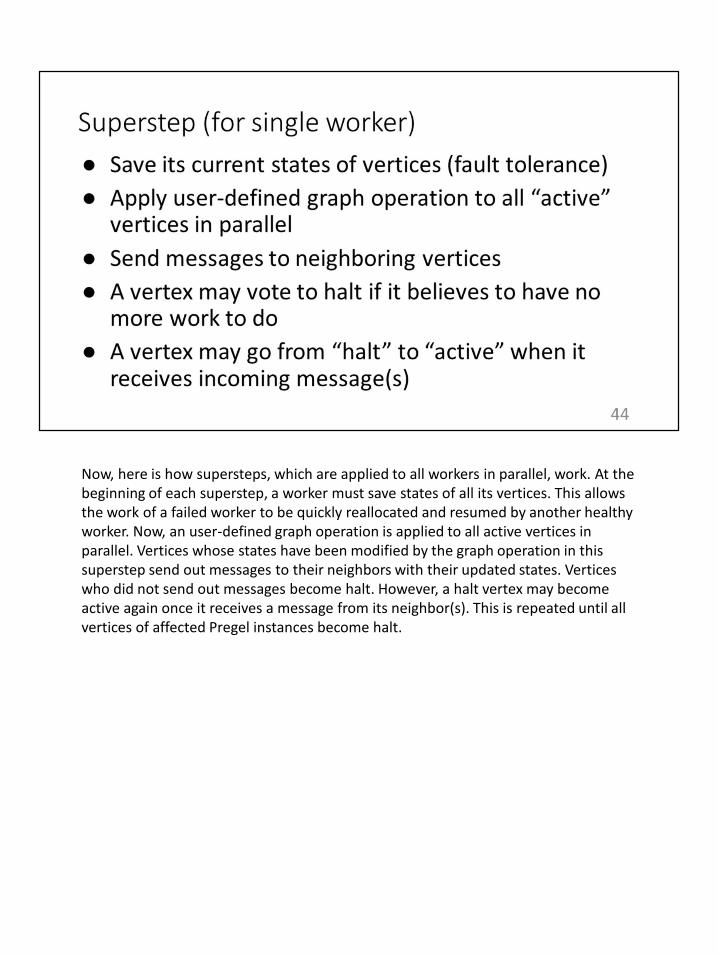
Now, here is how supersteps, which are applied to all workers in parallel, work. At the beginning of each superstep, a worker must save states of all its vertices. This allows the work of a failed worker to be quickly reallocated and resumed by another healthy worker. Now, an user-defined graph operation is applied to all active vertices in parallel. Vertices whose states have been modified by the graph operation in this superstep send out messages to their neighbors with their updated states. Vertices who did not send out messages become halt. However, a halt vertex may become active again once it receives a message from its neighbor(s). This is repeated until all vertices of affected Pregel instances become halt.

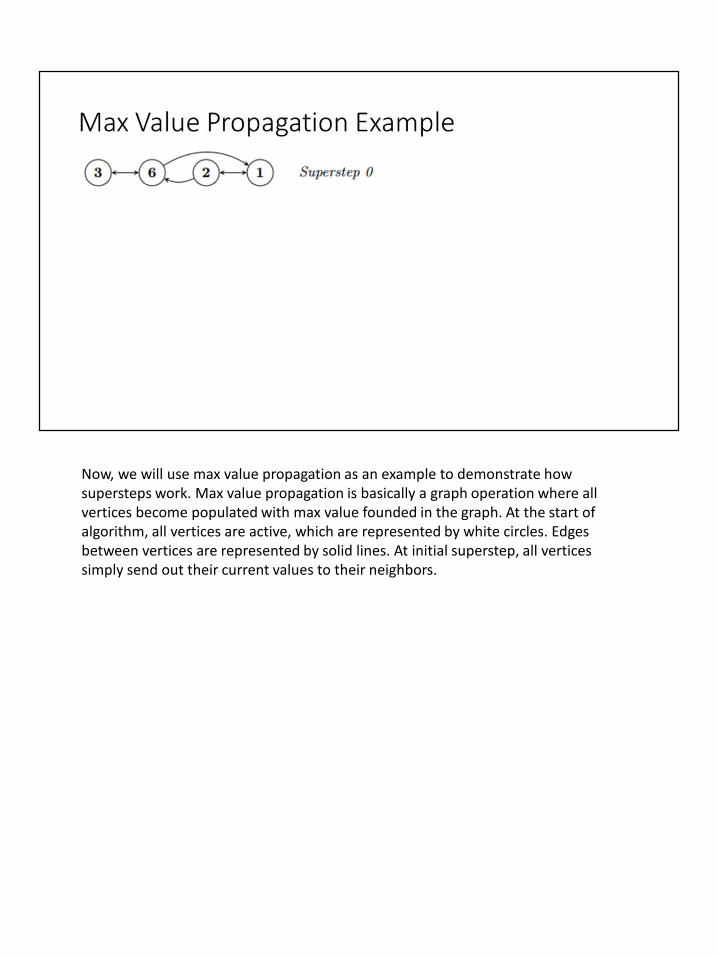
Now, we will use max value propagation as an example to demonstrate how supersteps work. Max value propagation is basically a graph operation where all vertices become populated with max value founded in the graph. At the start of algorithm, all vertices are active, which are represented by white circles. Edges between vertices are represented by solid lines. At initial superstep, all vertices simply send out their current values to their neighbors.

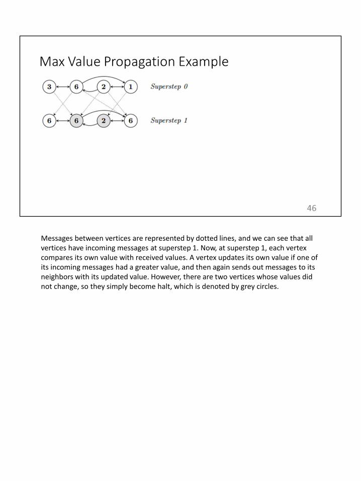
Messages between vertices are represented by dotted lines, and we can see that all vertices have incoming messages at superstep 1. Now, at superstep 1, each vertex compares its own value with received values. A vertex updates its own value if one of its incoming messages had a greater value, and then again sends out messages to its neighbors with its updated value. However, there are two vertices whose values did not change, so they simply become halt, which is denoted by grey circles.

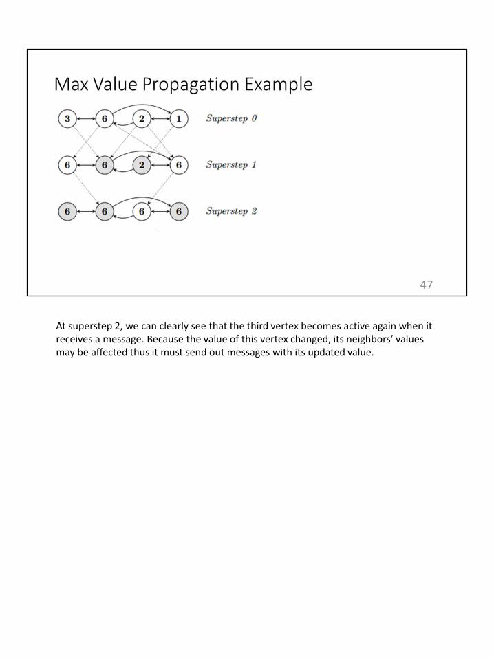
At superstep 2, we can clearly see that the third vertex becomes active again when it receives a message. Because the value of this vertex changed, its neighbors’ values may be affected thus it must send out messages with its updated value.

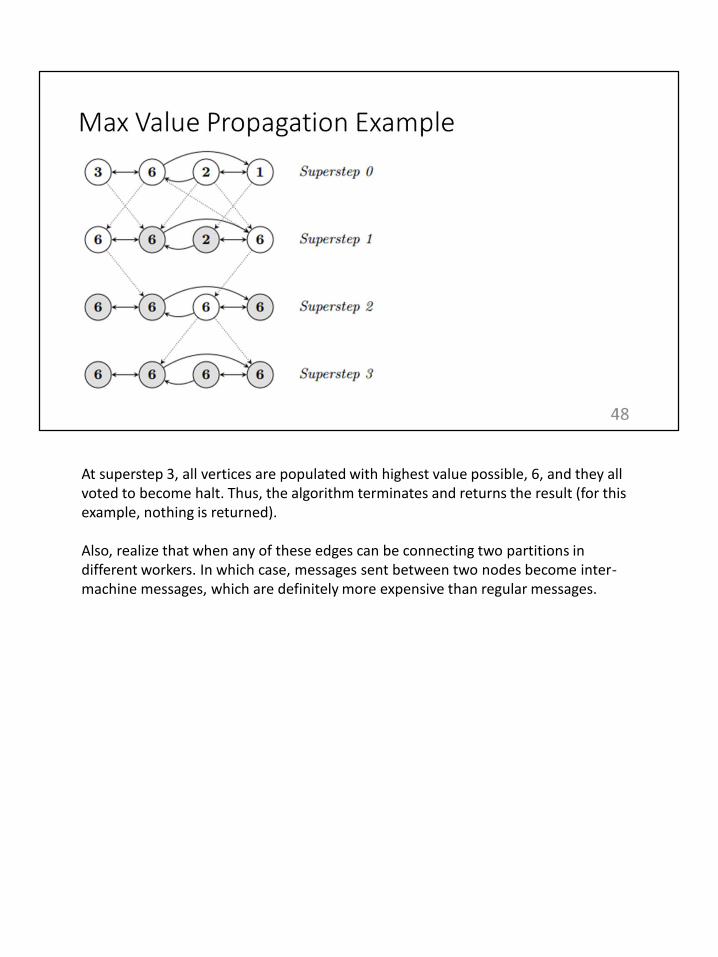
At superstep 3, all vertices are populated with highest value possible, 6, and they all voted to become halt. Thus, the algorithm terminates and returns the result (for this example, nothing is returned).

Also, realize that when any of these edges can be connecting two partitions in different workers. In which case, messages sent between two nodes become inter-machine messages, which are definitely more expensive than regular messages.

We mentioned that during the initialization step, Pregel divides a graph into partitions and distribute them among workers. To do this, Pregel simply computes the hash of each vertex, mod the resulting hash by the number of partitions, and then assign the vertex to partition based on that number. This results in non-optimal partitions, which obviously hurts the performance of a distributed graph database system since more messages sent during each superstep become inter-machine messages.

Sedge is a Pregel-based graph partition management system that minimizes these inter-machine communications in order to decrease the average query response time and increase the overall query throughput. Furthermore, Sedge dynamically repartition graphs based on workloads and query types in order to maximize parallelism while processing queries.

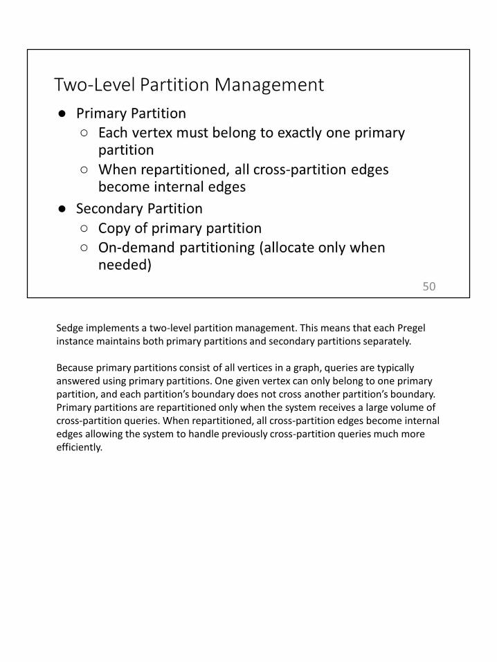
Sedge implements a two-level partition management. This means that each Pregel instance maintains both primary partitions and secondary partitions separately.

Because primary partitions consist of all vertices in a graph, queries are typically answered using primary partitions. One given vertex can only belong to one primary partition, and each partition’s boundary does not cross another partition’s boundary. Primary partitions are repartitioned only when the system receives a large volume of cross-partition queries. When repartitioned, all cross-partition edges become internal edges allowing the system to handle previously cross-partition queries much more efficiently.

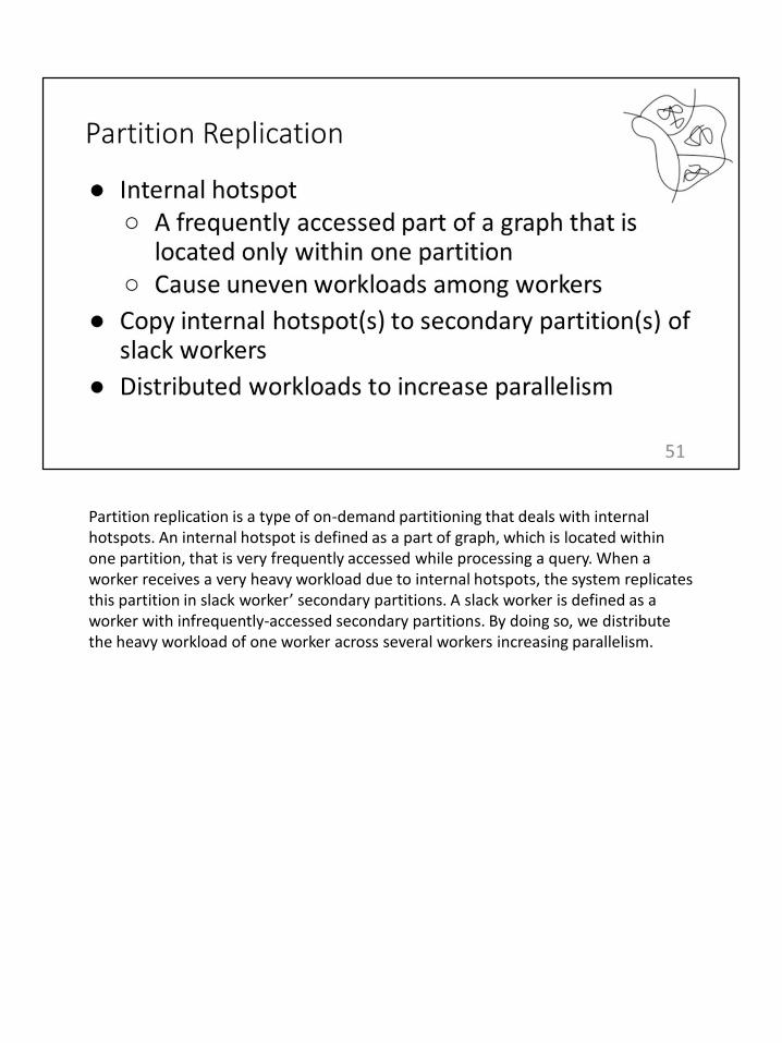
Partition replication is a type of on-demand partitioning that deals with internal hotspots. An internal hotspot is defined as a part of graph, which is located within one partition, that is very frequently accessed while processing a query. When a worker receives a very heavy workload due to internal hotspots, the system replicates this partition in slack worker’ secondary partitions. A slack worker is defined as a worker with infrequently-accessed secondary partitions. By doing so, we distribute the heavy workload of one worker across several workers increasing parallelism.

A cross-partition hotspot is basically an internal hotspot that spans on more than one partition. In addition to causing heavy workloads on few workers, a cross-partition hotspot forces those workers to much more frequently communicate with each other. In order to resolve this issue, Sedge generates a new partition covering the cross-partition hotspot and allocates it to secondary partitions of several slack workers. Now, the cross-partition hotspot is handled by a single machine effectively reducing the communication overhead.

53

The reason to present these slides were to given an idea of how to use Neo4j to represent a highly complicated social networking application where the graph structure itself gets modified over time. However, since we are already presenting simple examples of how to represent queries using Cypher, I don’t think this part of the presentation is justified. We can remove this and include a brief presentation of how relational DBs can be better used to represent a graph by using a graph abstraction keeping the underlying storage the same, just to provide a different perspective.

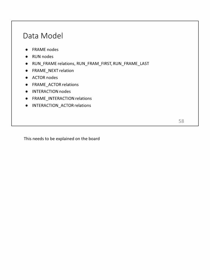
This needs to be explained on the board

Here we go into more detail as to why the authors chose Neo4j as a representative of graph DBs. Relational DBs have been around for quite a bit so most of the systems chosen would be mature so no justification for choosing PostgreSQL was made.