guidelines on analysis of extremes in a changing climate ... · 6.2 climate change detection and...
TRANSCRIPT

For more information, please contact:
World Meteorological Organization
Observing and Information Systems DepartmentTel.: +41 (0) 22 730 82 68 – Fax: +41 (0) 22 730 80 21
E-mail: [email protected]
7 bis, avenue de la Paix – P.O. Box 2300 – CH 1211 Geneva 2 – Switzerland
www.wmo.int
Guidelines on Analysis of extremes in a changing climate in support of informed decisions for adaptation
Climate Data and Monitoring WCDMP-No. 72
WMO-TD No. 1500

© World Meteorological Organization, 2009
The right of publication in print, electronic and any other form and in any language is reserved by WMO. Short extracts from WMO publications may be reproduced without authorization, provided that the complete source is clearly indicated. Editorial correspondence and requests to publish, reproduce or translate these publication in part or in whole should be addressed to:
Chairperson, Publications BoardWorld Meteorological Organization (WMO)7 bis, avenue de la Paix Tel.: +41 (0) 22 730 84 03P.O. Box 2300 Fax: +41 (0) 22 730 80 40CH-1211 Geneva 2, Switzerland E-mail: [email protected]
This publication was adapted with the permission of Environment Canada.
NOTE
The designations employed in WMO publications and the presentation of material in this publication do not imply the expression of any opinion whatsoever on the part of the Secretariat of WMO concerning the legal status of any country, territory, city or area, or of its authorities, or concerning the delimitation of its frontiers or boundaries.
Opinions expressed in WMO publications are those of the authors and do not necessarily reflect those of WMO. The mention of specific companies or products does not imply that they are endorsed or recommended by WMO in preference to others of a similar nature which are not mentioned or advertised.
June 2009
Guidelines on Analysis of extremes in a changing climate in support of informed decisions for adaptation
Albert M.G. Klein Tank*, Royal Netherlands Meteorological Institute
Francis W. Zwiers* and Xuebin Zhang, Environment Canada
* co-Chairs of the Joint CCl/CLIVAR/JCOMM Expert Team on Climate Change Detection and Indices (ETCCDI, see http://www.clivar.org/organization/etccdi/etccdi.php), whose aims are to provide international coordination and help organize collaboration on climate change detection and indices relevant to climate change detection; further develop and publicize indices and indicators of climate variability and change from the surface and sub-surface ocean to the stratosphere; and encourage the comparison of modelled data and observations.
Page 2
Contents
Foreword................................................................................................................................................ 3
Acknowledgements .............................................................................................................................. 4
1 Introduction ........................................................................................................................................ 5 1.1 The rationale for focusing on weather and climate extremes ............................................... 5 1.2 Objective .............................................................................................................................. 7 1.3 Scope................................................................................................................................... 7
2 Data preparation................................................................................................................................. 9 2.1 Long and quality-controlled daily observational series ......................................................... 9 2.2 Homogeneity...................................................................................................................... 11
3 Analysing extremes ......................................................................................................................... 14 3.1 Descriptive indices of extremes ......................................................................................... 14 3.2 Statistical modelling of extremes........................................................................................ 18 3.3 Scaling issues .................................................................................................................... 24
4 Assessing changes in extremes..................................................................................................... 25 4.1 Trends in climate indices of moderate extremes................................................................ 25 4.2 Changes in rare extreme events ........................................................................................ 31
5 Future extremes ............................................................................................................................... 36 5.1 Evidence of changes in extremes from observations ......................................................... 36 5.2 Evidence of changes in extremes from climate model projections ..................................... 37 5.3 Information services on future extremes ............................................................................ 38
6 Measures to further improve our understanding .......................................................................... 40 6.1 Data rescue, collection, digitization, and sharing ............................................................... 40 6.2 Climate change detection and attribution ........................................................................... 41
7 Wider societal benefits .................................................................................................................... 43
References........................................................................................................................................... 45
Appendix: ETCCDI indices................................................................................................................. 49

Page 3
Foreword The World Meteorological Organization (WMO) works collectively with its 188 Members to provide an authoritative voice on the Earth’s climate system. These efforts have led to the implementation of several products that provide regular information on the status of the global climate system, including products that monitor the occurrence of extreme weather and climate events. World Meteorological Congress XV recognized the increasing importance that Members are placing on monitoring, assessing and predicting the climate system at various space and time scales. In addition, it stressed the importance of high-quality climatologically observations and data sets for understanding and monitoring climate variability and change and urging Members to enhance climate monitoring capabilities for the generation of new and improved products and services. This even greater emphasis on climate continues a trend that has emerged over the past several decades whereby WMO has gradually increased the priority that it has given climate issues, following the World Climate Conferences in 1979 and 1990, each of which led to the creation of key climate programmes and bodies such as the World Climate Program (WCP), Global Climate Observing System (GCOS) as well as the Intergovernmental Panel on Climate Change (IPCC). In this context with the rapidly evolving WMO role and duties in climate, WMO’s Commission for Climatology (CCl), the World Climate Research Program (WCRP) with Climate Variability and Predictability (CLIVAR), and the Joint WMO-IOC Technical Commission for Oceanography and Marine Meteorology (JCOMM) have worked jointly to advance knowledge on climate change and extremes using scientifically computed statistics (indices) by undertaking scientific research, developing tools for the analysis of indices, and organizing capacity building workshops. I would like to congratulate the experts of the CCl/CLIVAR/JCOMM Team on Climate Change Detection and Indices (ETCCDI) for their excellent work in providing the scientific coordination of a number of regional workshops in all WMO regions and publishing high standard publications including this one. Addressing the observed as well as future changes in extremes is very pertinent approach taken in this publication. It well reflects that in the changing climate, past climate information is not sufficient to provide reliable indications for the future climate. The publication of such highly scientific material will further assist National Meteorological and Hydrological Services (NMHSs) and other climate-related institutions in providing scientific information in support of informed decisions in adaptating to climate variability and change. Finally, this publication is timely as the third World Climate Conference (WCC-3), scheduled to take place from 31 August to 4 September 2009, which will decide on a new framework for improved climate information and services. (M. Jarraud) Secretary-General

Page 4
Acknowledgement
This guidelines document follows on a workshop in De Bilt, The Netherlands, 13–16 May 2008, which was organized jointly by CCL/CLIVAR/JCOMM-ETCCDI and the European Union project ENSEMBLES (www.ensembles-eu.org). It constitutes one of the major actions of the ETCCDI work plan for 2006–2009 that was developed during a meeting in Niagara-on-the-Lake, Canada, 14–16 November 2006. We thank Pierre Bessemoulin for highlighting the importance of non-stationarity in extremes analysis. We also wish to express our thanks to Omar Baddour, Jules Beersma, Else van den Besselaar and Adri Buishand for comments on an earlier version of this document.

Page 5
1 Introduction
1.1 The rationale for focusing on weather and climate extremes
Changes in extreme weather and climate events have significant impacts and are among the most serious challenges to society in coping with a changing climate (CCSP, 2008). Indeed, ”confidence has increased that some extremes will become more frequent, more widespread and/or more intense during the 21st century” (IPCC, 2007). As a result, the demand for information services on weather and climate extremes is growing. The sustainability of economic development and living conditions depends on our ability to manage the risks associated with extreme events.
Many practical problems require knowledge of the behaviour of extreme values. In particular, the infrastructures we depend upon for food, water, energy, shelter and transportation are sensitive to high or low values of meteorological variables. For example, high precipitation amounts and resulting stream flows affect sewerage systems, dams, reservoirs and bridges. The motivation for analysing extremes is often to find an optimum balance between adopting high safety standards that are very costly on the one hand, and preventing major damage to equipment and structures from extreme events that are likely to occur during the useful life of such infrastructure on the other hand (WMO, 1983).
Most existing systems for water management and other infrastructure have been designed under the assumption that climate is stationary. This basic concept from which engineers work assumes that climate is variable, but with variations whose properties are constant with time, and which occur around an unchanging mean state. This assumption of stationarity is still common practice for design criteria for (the safety of) new infrastructure, even though the notion that climate change may alter the mean, variability and extremes of relevant weather variables is now widely accepted. New infrastructure is typically designed on the basis of historical information on weather and climate extremes. Often, the maximum value of a particular variable in the historical record is considered to be the normative value for design. In other cases, extreme value theory is applied to the historical observations of extremes to estimate the normative value, again disregarding climate change.
It is possible to account for non-stationary conditions (climate change) in extreme value analysis, but scientists are still debating the best way to do this. Nevertheless, adaptation strategies to climate change should now begin to account for the decadal scale changes (or low-frequency variability) in extremes observed in the past decades, as well as projections of future changes in extremes such as are obtained from climate models. Some types of infrastructure currently have little margin to buffer the impacts of climate change. For example, a recent evaluation (Ten Brink and others, 2008) indicates that at least 15 per cent of the primary dyke system in the Netherlands does not meet the safety standards as set down in Dutch national law due to increasing sea height extremes associated with rising sea levels. In other cases, projected changes (although highly uncertain) are so large that simply relying on traditional methods of extremes estimation would no longer appear to be prudent. Indeed, the climate change signal is already clearly distinguishable in many variables (Hegerl and others, 2007).

Page 6
It should be pointed out that the creation of an efficient early warning system for climate anomalies and related extremes has been a focus of the World Meteorological Organization (WMO) and the National Meteorological and Hydrological Services (NMHSs) for more than a decade in order to improve climate risk management capabilities among nations (Zhai and others, 2005). To this effect, NMHSs should be adequately equipped and prepared to continuously monitor, assess and provide information on the state of the climate and its departure from the historical climate averages with reference to the observed extreme values of weather and climate variables.
According to the International Panel on Climate Change (IPCC) (2007), most of the observed increase in global average temperatures since the mid-twentieth century is very likely due to the observed increase in anthropogenic greenhouse gas concentrations. Discernible human influences now extend to other aspects of climate, including ocean warming, continental-average temperatures, temperature extremes, and wind patterns (IPCC, 2007). Evidence that human influence is affecting many aspects of the hydrological cycle on global and even regional scales is now accumulating (for example Zhang and others, 2007; Santer and others, 2007; Min and others, 2008; Barnett and others, 2008; Milly and others, 2008). These changes in mean state inevitably affect extremes. Moreover, the extremes themselves may be changing in such a way as to cause changes that are larger than would simply result from a shift of variability to a higher range (Hegerl and others, 2004; IPCC, 2007; Kharin and others, 2007).
The overall question addressed in this guidelines document is how we should account for a changing climate when assessing and estimating extremes. Pertinent points include how to incorporate observed changes in extremes in the past in the analysis; and determining the best way to deal with available future climate model projections.
This document is structured as follows. Chapter 1 details the objective and scope. Chapter 2 describes data preparation and quality control, which are necessary steps before any extremes analysis. Chapter 3 explains the basic concept of extremes indices and the traditional approach of statistical modelling of extremes, assuming stationary conditions. Chapter 4 describes methods to assess changes in extremes to account for non-stationarity. Chapter 5 provides an overview of reported changes in observations and climate model projections, and more importantly, how this information, together with the methods described in the earlier chapters, can be used to improve the information services on future extremes. Finally, in Chapter 6 measures to improve our understanding are highlighted, and in Chapter 7 the wider societal benefits of extremes analysis are described. Note that each paragraph ends with a textbox, which summarizes the main message.
Climate change makes it likely that there will be change in some extremes that lie outside the envelope of constant variability assumed under stationary climate conditions. It is possible to account for this “non-stationarity”, but the best way to do this is still under debate. Nevertheless, adaptation strategies should begin to take into account the observed and projected changes in extremes. The key question addressed in this guidelines document is how to account for a changing climate when assessing and estimating weather and climate extremes.

Page 7
1.2 Objective
This guidelines document is targeted at NMHSs around the world that need to deal with practical questions on extremes and provide information services for climate change adaptation strategies (see WMO, 2007a). It responds to the need of WMO Members to enhance climate monitoring capabilities for the generation of higher quality and new types of products and services (Resolution 12 (Cg-XV)).
Many NMHSs already provide practical information services on weather extremes, such as frequency tables for the occurrence of extremes and maps of return periods of extremes (average waiting times between the occurrences of extremes of a fixed size). They are generally aware of climate change, but find it difficult to include this notion and the available scientific results in their services and products. The aim of this document is to help build capacity in NMHSs to identify and describe changes in extremes, and to improve the information services on extremes under climate change conditions. In this way, NMHSs will become better equipped to answer questions such as whether extremes in their specific regions have changed and to communicate such knowledge to their clients, the end users. Knowledge of changes in weather and climate extremes is essential to manage climate-related risks to humans, ecosystems and infrastructure, and develop resilience through adaptation strategies.
This document, which is targeted at National Meteorological and Hydrological Services (NMHSs) around the world, aims to help build capacity to identify and describe changes in extremes, and to improve information services on extremes under climate change conditions.
1.3 Scope
This document is not intended to form a comprehensive textbook on extremes. Rather, some selected key issues related to assessing changes in weather and climate extremes will be discussed. Several examples of practical applications will also be given.
The scientific debate on the best way to assess changes in weather and climate extremes is still ongoing, but guidance on a number of topics can and will be provided, including:
(a) Preparation of data series (in particular observations) for the analysis of extremes; (b) Utilization of descriptive indices and extreme-value theory to evaluate extremes; (c) Trend calculation and other statistical approaches for assessing changes in extremes; (d) Assessment of observed changes and model projected changes in extremes.
It is important to note that this guide does not cover every type of extreme. It focuses on weather and climate extremes that are defined as rare events within the statistical reference distribution of particular weather elements at a particular place (Houghton and others, 2001). The extremes in this guide are for weather elements that are monitored daily, such as temperature and precipitation. Additional factors that fall outside the scope of this guide must be taken into consideration when evaluating changes in more

Page 8
complicated phenomena, such as tropical cyclones or storm surges. Nevertheless, evaluating the extremes of basic weather elements and determining whether they are changing are fundamental first steps that are necessary to enhance the capacity to analyse extremes.
The focus on rare events within the statistical reference distribution of particular weather elements at a particular place means that we do not concentrate solely on the extremes that cause the largest socio-economic losses and the greatest impacts as reported in the media. The impacts that result from extreme values of weather elements are to a large degree dependent on the conditions of the system that is under investigation (including its vulnerability or resilience). For instance, the hydrology of an area and prior conditions determine whether a heavy rainfall event turns into a flood. Likewise, the design of buildings, availability of cooling equipment, and local socio-economic conditions determine whether communities can withstand summer heatwaves. Although weather extremes are not directly related to environmental disasters (damaging impacts can also occur in the absence of a very rare or intense climatic event), a systematic change in weather extremes will very likely also be accompanied by a systematic change in hazardous weather conditions that have adverse effects on ecosystems or sectors of society (human safety and health, water management, agriculture, energy, insurance, tourism and transport).
From a scientific point of view, assessing changes in extreme impact events (or environmental disasters) rather than extremes in the tails of the statistical distribution can be problematic for several reasons. First, the inventories that are available to study extreme impact events (see Cornford, 2003) are biased towards recent years simply because of improved communication technology. Second, methods to compare reported events in an objective way considering biases are lacking. Third, even when corrected for improving communication technology, the growing number of reported events may reflect factors such as global trends in population vulnerability as well as an increased frequency of extreme events.
Rather than forming a comprehensive textbook on extremes, this guide will cover some selected key issues, including examples of practical applications. The focus is on weather and climate extremes defined as rare events within the statistical reference distribution of particular weather elements that are monitored daily at a particular place, such as temperature and precipitation. More complicated weather elements that involve compound factors, such as tropical cyclones or storm surges, fall outside the scope of this guide. Although the extremes in the tails of the distribution are not directly related to environmental disasters, it is very likely that a systematic change in weather extremes will also be accompanied by a systematic change in extreme impact events.

Page 9
2 Data preparation
2.1 Long and quality-controlled daily observational series
Assessing changes in extremes is not trivial. For statistical reasons, a valid analysis of extremes in the tails of the distribution requires long time series to obtain reasonable estimates of the intensity and frequency of rare events, such as the 20-year return value (an event whose intensity would be exceeded once every 20 years, on average, in a stationary climate). Also, continuous data series with at least a daily time resolution are needed to take into account the sub-monthly nature of many extremes. This requirement may be particularly problematic because, in various parts of the globe, there is a lack of high-quality daily observation records covering multiple decades that are part of integrated data sets.
As noted in IPCC (2007), in many regions of the world it is not yet possible to make firm assessments of how global warming has affected extremes. As a result, far less is known about past changes in extremes than past changes in mean climate. This is because observational time series are generally not available in the required high time resolution digital form. Consequently, the limited spatial coverage of the available data sets with high enough resolution (at least daily values) often hampers regional assessments. Even where the necessary data are available, systematic changes in extremes may be difficult to detect locally if there is a large amount of natural inter-annual variability in extremes.
WMO guidance on developing long-term, high-quality and reliable instrumental climate records is provided in Brunet and others (2008). Basic quality control (QC) usually involves a variety of graphical and statistical analyses. A worldwide series of capacity-building workshops for monitoring weather and climate extremes have been organized by the ETCCDI and the Asia-Pacific Network for Global Change Research (APN; Peterson and Manton, 2008). These regional workshops continue to be undertaken whenever opportunity and resources allow. The core component of each such workshop is a hands-on analysis of national observational data with daily resolution, which have often never been analysed prior to the workshop. The example below draws from the standard QC analysis techniques used in these workshops. The software provided for this purpose, which uses the open source statistical programming language R (www.r-project.org), is freely available from http://cccma.seos.uvic.ca/ETCCDI and comes with a tutorial. A graphical user interface is provided, so knowledge of R is not necessarily required. Nevertheless, knowledge of R allows users to read and understand the software and to make modifications, such as might be needed to accommodate national data management standards.
Example
The first step is assembling available data and selecting the candidate station series for extremes analysis on the basis of series length and data completeness. In many daily resolution climatic time series, a number of observation days are missing. A frequently used completeness criterion allows for at most four missing observations per year. Such a strict criterion is needed because some extremes analyses are critically dependent on the serial completeness of the data. A particular concern regarding missing observation days in the case of an extremes analysis is that an extreme event might have been responsible for the failure of the observing system and thus the fact that the observation for that day is

Page 10
missing; such “censoring” of extremes would result in negatively biased estimates of the intensity of rare events, such as the 20-year event.
The main purpose of the subsequent QC procedure is to identify errors usually caused by data processing such as manual keying. In many series, obviously wrong values, such as nonexistent dates, need to be removed. Negative daily precipitation amounts are set to missing values, and both daily maximum and minimum temperatures are set to missing values if the daily maximum temperature is less than the daily minimum temperature.
Next, the QC procedure identifies outliers in daily maximum and minimum temperatures and precipitation amounts. Outliers are daily values that lie outside a particular range defined as unrealistic by the user. For example, for temperature series, this range can be defined as the mean value of observations for the day of the year plus or minus four times the standard deviation of the value for that calendar day in the entire series. Daily temperature values outside of these thresholds are marked as potentially erroneous, and manually checked and corrected on a case-by-case basis. Each potential outlier can be evaluated using information from the days before and after the event along with expert knowledge about the local climate. For precipitation, outliers can be the result of several days’ accumulation of missing observations. Suspiciously long spells of zero precipitation values may also be indicative of a time series where multi-day accumulated values have been included in the daily time series or where missing values have been given the value zero. If a nearby station is available, then outliers can be compared across stations. Great care must be taken in determining whether identified outliers are truly erroneous because their inclusion, adjustment, or exclusion can profoundly affect subsequent extremes analyses.
Although statistical tests are important for QC, visual checks of data plots can also reveal outliers as well as a variety of problems that cause changes in the seasonal cycle or changes in the variance of the data. In addition, histograms or so-called stem and leaf plots (Wilks, 1995) of the data reveal problems that show up when the data set is examined as a whole. Those extreme temperature and precipitation observations that are positively identified as wrong are best removed from the time series (i.e. set to missing values) unless there is an obvious cause of the error, such as a transcription of digits or misplacement of a decimal point, which allows it to be confidently corrected.
Observational data series with an excessive number of problems (typically three or more) that are not easily solved are best left out of the analysis entirely.
Long-term, high-quality and reliable climate records with a daily (or higher) time resolution are required for assessing changes in extremes. WMO guidance on developing such data sets for observations is provided in Brunet and others (2008). The ETCCDI makes standardized software tools available to perform basic quality control analysis from http://cccma.seos.uvic.ca/ETCCDI.

Page 11
2.2 Homogeneity
Once data have been quality controlled, it is necessary to assess their temporal homogeneity. Climatic time series often exhibit spurious (non-climatic) jumps and/or gradual shifts due to changes in station location, environment (exposure), instrumentation or observing practices. In addition, the time series from some city stations include urban heating effects, as well as discontinuities resulting from station relocations to out-of-town airports. These inhomogeneities may severely affect the extremes. The station history metadata are vital for resolving these issues.
Experts from different parts of the world have produced a list of classical examples of inhomogeneities (http://cccma.seos.uvic.ca/ETCCDI/example.shtml) in observational series. These examples illustrate the main causes of the inhomogeneities and their possible impacts on climate trend analysis.
Many approaches and statistical techniques have been developed for evaluating the homogeneity of climate time series and for detecting and adjusting inhomogeneities (for an overview, see Aguilar and others, 2003). Nevertheless, further research is required to fully address this difficult issue for high-resolution daily time series. At the moment, there are no established methods to determine and adjust inhomogeneities in daily resolution time series, although some techniques are under development, for example see Brandsma (2001), Vincent and others (2002), Della-Marta and Wanner (2006). In Europe, the European Cooperation in Science and Technology mechanism (COSTHOME) compares the performance of different methods for homogenization of long instrumental daily climate records (see http://www.homogenisation.org/), but conclusive results are not yet available. If the available number of records and station density so allow, the safest solution is to remove time series with indications of artificial changes from the analysis altogether. As an alternative, one can decide to use only the part of the series with indications of discontinuities of non-climatic origin that occurs after the time of the last discontinuity. Nevertheless, there may be instances when the use of adjusted time series will be unavoidable, such as in countries or regions with low station density.
In the European Climate Assessment & Dataset project (ECA&D; http://eca.knmi.nl), a combination of different statistical tests developed for testing monthly resolution time series was used to evaluate the properties of daily series. This allowed a ranking of these series (see Wijngaard and others, 2003) which can help users to decide which series should be retained for a particular application. The example below is for Canada and is drawn from the expert list of classical examples. it illustrates the use of one particular statistical test which, although developed for homogeneity testing of lower than daily resolution time series, has been successfully applied in the series of workshops organized by ETCCDI. The two-phase regression-based test is part of the homogeneity-testing software program RHtestV2, which is available from the ETCCDI website. It also uses the open source statistical programming language R, and has a graphical user interface.
Example
This example, which is presented in Vincent and others (2002), describes how inhomogeneities were identified in the minimum temperature series of Amos (Canada, 48°34’N, 78°07’W) using RHtestV2. This program consists of a series of R functions to detect and adjust for multiple change-points (shifts in

Page 12
the mean) in a series. It is based on the penalized t-test (Wang and others, 2007) and the penalized maximal F-test (Wang, 2008a).
-3
-2
-1
0
1
2
3
1910 1920 1930 1940 1950 1960 1970 1980 1990 2000
°C
1927 1963
Figure 1: Example of data inhomogeneity in the annual average daily minimum temperature series (anomalies relative to a reference series computed from surrounding stations) for station Amos (Canada). On the basis of the two-phase regression model implemented in RHtestV2, two change-points (inhomogeneities) are detected for the years 1927 and 1963.
Figure 2: Screen location at station Amos (Canada) before 1963 (left) and after 1963 (right).
These tests account for various problems that often affect the methods used for homogeneity analysis. For example, the effects of day-to-day persistence of observations on the properties of these statistical tests are accounted for empirically (Wang, 2008b). The possibility that the time series being tested may have a linear trend throughout the period of record is also taken into account, and measures have been taken to ensure that change-points are detected with consistent reliability throughout the length of the time series. A homogeneous time series that is well correlated with the candidate series has been used
Page 13
as a reference series. However, detection of change-points is also possible if a homogeneous reference series is not available.
RHtestV2 is applied to the annual means of the daily minimum temperature series to identify likely inhomogeneities in the data. Once a possible change-point has been identified in the annual series, it is also checked against station history metadata records, if available. Figure 1 shows the result for Amos where two change-points have been detected in the series between 1915 and 1995: a step of -0.8°C in 1927 and a step of 1.3°C in 1963. The station history files revealed that the Stevenson screen was located at the bottom of a hill prior to 1963 and was moved onto level ground, several metres away from its original position, after 1963 (Figure 2). The former site was sheltered by trees and buildings which could have prevented the cold air from draining freely at night time. The current site has better exposure and the observations are more reliable. The station history files do not provide any information on the cause of the first step. In this case, it is best to use only the part of the series after the second discontinuity for the analysis of extremes.
Many approaches and statistical techniques have been developed for detecting inhomogeneities in climatological time series and adjusting data sets (for an overview, see Aguilar and others, 2003). Nevertheless, further research is required to fully address this difficult issue for high-resolution daily time series. The general recommendation is to use a number of different techniques to identify potential discontinuities and, where possible, to obtain confirmation from the metadata. If the available number of records and the station density allow, the safest solution is to remove time series with indications of artificial changes from the extremes analysis altogether.

Page 14
3 Analysing extremes
3.1 Descriptive indices of extremes
To gain a uniform perspective on observed changes in weather and climate extremes, ETCCDI has defined a core set of descriptive indices of extremes. The indices describe particular characteristics of extremes, including frequency, amplitude and persistence. The core set includes 27 extremes indices for temperature and precipitation. The specifications for these indices are given in the Appendix. User-friendly R-based software (RClimDex) for their calculation is available from http://cccma.seos.uvic.ca/ETCCDI.
One of the key approaches of the indices concept involves calculation of the number of days in a year exceeding specific thresholds. Examples of such “day-count” indices are the number of days with minimum temperature below the long-term 10th percentile in the 1961-1990 base period or the number of days with rainfall amount higher than 20 mm. Many ETCCDI indices are based on percentiles with thresholds set to assess moderate extremes that typically occur a few times every year rather than high-impact, once-in-a-decade weather events. For precipitation, the percentile thresholds are calculated from the sample of all wet days in the base period. For temperature, the percentile thresholds are calculated from five-day windows centered on each calendar day to account for the mean annual cycle. Such indices allow straightforward monitoring of trends in the frequency or intensity of events, which, while not particularly extreme, would nevertheless be stressful. The reason for choosing mostly percentile thresholds rather than fixed thresholds is that the number of days exceeding percentile thresholds is more evenly distributed in space and is meaningful in every region.
Day-count indices based on percentile thresholds are expressions of anomalies relative to the local climate. These anomalies have fixed rarity, that is, the thresholds are chosen so as to be exceeded at a fixed frequency, often 10 per cent, during the base period that is used to define the thresholds. Consequently, the values of the thresholds are site-specific. Such indices allow for spatial comparisons because they sample the same part of the probability distribution of temperature and precipitation at each location. Day-count indices based on absolute thresholds are less suitable for spatial comparisons of extremes than those based on percentile thresholds. The reason is that, over large areas, day-count indices based on absolute thresholds may sample very different parts of the temperature and precipitation distributions. For annual indices, this implies that in another climate regime, the variability in such indices readily stems from another season. For instance, year-to-year variability in frost-day counts (days with minimum temperature below 0°C) relates to the variability in the spring and autumn temperatures for the northern part of the Northern Hemisphere midlatitudes, whereas in the southern part of the Northern Hemisphere midlatitudes, annual variability in frost-day counts is determined by winter temperature variability. Likewise, the 25°C threshold used in the definition of “summer” days (days with maximum temperature above 25°C) samples variations in summer temperatures at high latitudes and variations in spring and autumn temperatures at lower latitudes.
Values of absolute extremes, such as the highest five-day precipitation amount in a year (RX5day), can often be related to extreme events that affect human society and the natural environment. Indices based
Page 15
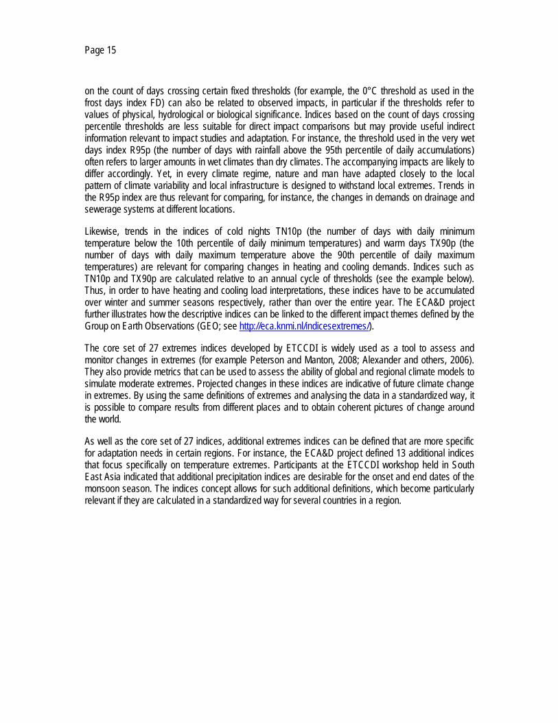
on the count of days crossing certain fixed thresholds (for example, the 0°C threshold as used in the frost days index FD) can also be related to observed impacts, in particular if the thresholds refer to values of physical, hydrological or biological significance. Indices based on the count of days crossing percentile thresholds are less suitable for direct impact comparisons but may provide useful indirect information relevant to impact studies and adaptation. For instance, the threshold used in the very wet days index R95p (the number of days with rainfall above the 95th percentile of daily accumulations) often refers to larger amounts in wet climates than dry climates. The accompanying impacts are likely to differ accordingly. Yet, in every climate regime, nature and man have adapted closely to the local pattern of climate variability and local infrastructure is designed to withstand local extremes. Trends in the R95p index are thus relevant for comparing, for instance, the changes in demands on drainage and sewerage systems at different locations.
Likewise, trends in the indices of cold nights TN10p (the number of days with daily minimum temperature below the 10th percentile of daily minimum temperatures) and warm days TX90p (the number of days with daily maximum temperature above the 90th percentile of daily maximum temperatures) are relevant for comparing changes in heating and cooling demands. Indices such as TN10p and TX90p are calculated relative to an annual cycle of thresholds (see the example below). Thus, in order to have heating and cooling load interpretations, these indices have to be accumulated over winter and summer seasons respectively, rather than over the entire year. The ECA&D project further illustrates how the descriptive indices can be linked to the different impact themes defined by the Group on Earth Observations (GEO; see http://eca.knmi.nl/indicesextremes/).
The core set of 27 extremes indices developed by ETCCDI is widely used as a tool to assess and monitor changes in extremes (for example Peterson and Manton, 2008; Alexander and others, 2006). They also provide metrics that can be used to assess the ability of global and regional climate models to simulate moderate extremes. Projected changes in these indices are indicative of future climate change in extremes. By using the same definitions of extremes and analysing the data in a standardized way, it is possible to compare results from different places and to obtain coherent pictures of change around the world.
As well as the core set of 27 indices, additional extremes indices can be defined that are more specific for adaptation needs in certain regions. For instance, the ECA&D project defined 13 additional indices that focus specifically on temperature extremes. Participants at the ETCCDI workshop held in South East Asia indicated that additional precipitation indices are desirable for the onset and end dates of the monsoon season. The indices concept allows for such additional definitions, which become particularly relevant if they are calculated in a standardized way for several countries in a region.
Page 16
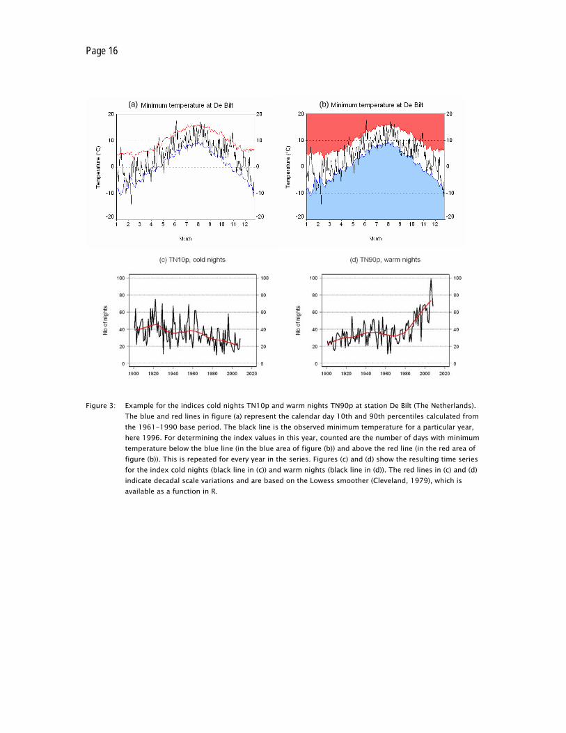
Figure 3: Example for the indices cold nights TN10p and warm nights TN90p at station De Bilt (The Netherlands). The blue and red lines in figure (a) represent the calendar day 10th and 90th percentiles calculated from the 1961-1990 base period. The black line is the observed minimum temperature for a particular year, here 1996. For determining the index values in this year, counted are the number of days with minimum temperature below the blue line (in the blue area of figure (b)) and above the red line (in the red area of figure (b)). This is repeated for every year in the series. Figures (c) and (d) show the resulting time series for the index cold nights (black line in (c)) and warm nights (black line in (d)). The red lines in (c) and (d) indicate decadal scale variations and are based on the Lowess smoother (Cleveland, 1979), which is available as a function in R.
(a) (b)

Page 17
Example
In this example, the indices for cold nights TN10p and warm nights TN90p are calculated based on the daily series of minimum temperature TN at station De Bilt (The Netherlands, 52°06’N, 05°11’E). Following the ETCCDI definitions, the numbers of cold and warm nights are calculated as follows (see Appendix):
10. TN10p, cold nights: count of days where TN < 10th percentile Let TNij be the daily minimum temperature on day i in period j and let TNin10 be the calendar day 10th percentile of daily minimum temperature calculated for a five-day window centred on each calendar day in the base period n (1961-1990). Count the number of days where TNij < TNin10.
12. TN90p, warm nights: count of days where TN > 90th percentile Let TNij be the daily minimum temperature on day i in period j and let TNin90 be the calendar day 90th percentile of daily minimum temperature calculated for a five-day window centred on each calendar day in the base period n (1961-1990). Count the number of days where TNij > TNin90.
Note that the periods j are typically one year in length, but other period lengths could be used, such as seasons defined as appropriate for the region that is being monitored. The values of the percentile thresholds are determined empirically from the observed station series in the climatological standard-normal period 1961–1990. The choice of another normal period (e.g. 1971–2000) has only a small impact on the results for the changes in the indices over time. The percentiles are calculated from five-day windows centred on each calendar day to account for the mean annual cycle. A five-day window is chosen to yield a total sample size of 30 years × 5 days = 150 for each calendar day, which results in a relatively smooth annual cycle of percentile thresholds. The procedure ensures that extreme temperature events, in terms of crossings of percentile thresholds, can occur with equal probability throughout the year (see Figure 3). The bootstrap procedure of Zhang and other (2005) has been implemented in RClimDex to ensure that the percentile-based indices do not have artificial jumps at the boundaries of the base period.
An internationally coordinated core set of 27 indices describes different aspects of moderate temperature and precipitation extremes, including frequency, intensity and duration. These indices are widely used for monitoring changes in extremes, climate model evaluation and assessments of future climate. One of the key approaches involves counting the number of days in a season or a year that exceed specific thresholds, in particular percentiles in the statistical distribution. The specifications for the 27 agreed indices are provided in the Appendix. Open source software for their calculation is available from http://cccma.seos.uvic.ca/ETCCDI.
Page 18
3.2 Statistical modelling of extremes
The descriptive indices developed by ETCCDI refer to moderate extremes that typically occur several times every year. Extreme value theory complements the descriptive indices in order to evaluate the intensity and frequency of rare events that lie far in the tails of the probability distribution of weather variables, say events that occur once in 20 years. In some engineering applications, such analysis requires estimation of events that are unprecedented in the available record, say events that occur once in a hundred or thousand years (extreme quantiles of the statistical distribution), while the observation series may be only about 50 years long.
For an introduction to extreme value theory one can read, amongst many publications, Coles (2001a), Smith (2002), or Katz and others (2002). The most common approach involves fitting a statistical model to the annual extremes in a time series of data. The WMO report entitled “Statistical Distributions for Flood Frequency Analysis” (WMO, 1989) provides an extensive review of probability distributions and methods for estimation of their parameters.
The extreme quantiles of interest to the analyst are generally estimated from an extreme value distribution. Two general methods can be used. One method, referred to as the “peaks-over-threshold” or POT method, is used to represent the behaviour of exceedances above a high threshold and the threshold crossing process. Under suitable conditions, and using a high enough threshold, extremes identified in this way will have a generalized Pareto, or GP, distribution (see, for example, Smith, 2002). Successful implementation of the POT method generally requires more decisions from the user (for example, declustering of extremes, specification of a sufficiently high threshold, dealing with the annual cycle, etc.) than the block maximum approach, which will be described next, but may use the information available in the observed data series more efficiently (Kharin and others, 2007). This could result in potentially more accurate estimates of extreme quantiles.
A second more generally used method based on an explicit extreme value theory is the so-called “block maximum” method. In this method, one considers the sample of extreme values obtained by selecting the maximum (or in some cases, the minimum) value observed in each block. Blocks are typically one year in length (365 daily observations per block), or occasionally a season in length (for example, the summer maximum temperature, or winter minimum temperature). Statistical theory indicates that the Generalized Extreme Value, or GEV, distribution is appropriate for the block maxima when blocks are sufficiently large. In its general form, the GEV distribution has three parameters: location, scale, and shape. Parameters can be estimated by the method of maximum likelihood (Jenkinson, 1955), the method of L-moments (Hosking, 1990; also referred to as probability weighted moments), or simply the ordinary method of moments. The maximum likelihood approach is preferred when samples of extremes are sufficiently large and when there is a possibility that the climate may not be stationary. In this case, the maximum likelihood method can include so-called “covariates” to incorporate the effects of non-stationarity on extremes (see Section 4.2). The method of L-moments is preferred when samples are small since in this case, maximum likelihood estimation of the parameters of the GEV distribution is not always successful (see, for example, Kharin and Zwiers, 2005). The ordinary method of moments, in which the mean, variance and skewness of the sample of extremes (block maxima) are matched to

Page 19
theoretical expressions for the mean, variance and skewness of the GEV distribution, is not recommended since it tends to underestimate long-period return values (Landwehr and others, 1979).
It is important to test the goodness-of-fit of the fitted distribution (see for example Kharin and Zwiers, 2000) and to assess the uncertainty of the estimates of the distribution’s parameters by calculating standard errors and confidence intervals for these estimates. The latter can be done in a relatively straightforward way when the distribution has been fitted by maximum likelihood because in this case the underlying statistical theory provides expressions that generally give good approximations for these quantities. Useful further evaluation of the results can be obtained by comparing the parametric estimates of quantiles for moderate return periods to the corresponding empirical estimates, for example, by comparing observed and estimated quantiles in a “quantile-quantile” plot, wherein observed and estimated quantiles are plotted against each other. This will help to identify the main sources of uncertainty, which may be related to the statistical techniques but depend particularly on the sample (especially the series length).
A specific problem in this context is how to deal with outliers that have been retained after careful quality control, assessment of available metadata and assessment of corroborating information such as published media reports. Such outliers, which could be much larger than any other observation in the record, presumably represent very well-documented events where the specific observation is not in doubt given the supporting metadata and other information. In such instances, the analyst may find that the fitted distribution is very sensitive to the inclusion or exclusion of the outlier, and goodness-of-fit statistics may indicate that the quality of the fit is reduced by its inclusion. Moreover, it is often the situation in such cases that if the outlier is excluded, estimated return values for return periods corresponding to the length of the record are smaller than the outlying observation. While there is clearly evidence that the chosen extreme value distribution does not fully describe all of the available, trusted, observations, it would nevertheless be prudent to include the outlier in the analysis and to take note of the possibility that return value estimates and associated confidence intervals may be subject to some error. In engineering hydrology practice, other evidence that can establish the return period of these outliers has been used to estimate empirical probability (or plotting position) of such events to improve the fit. Ignoring a well-documented extreme observation in the record to obtain an apparently better statistical fit would clearly yield unreliable return value estimates, given the evidence embodied by the outlying extreme, and is not recommended.
In addition to assessing goodness-of-fit by using a standard goodness-of-fit statistic or by examining a quantile-quantile plot, it is also important to assess whether the fitted distribution is “feasible”, meaning that all observed extremes should be possible under the fitted distribution (Dupuis and Tsao, 1998; Kharin and Zwiers, 2000). In the case of the GEV distribution, the shape parameter determines whether the fitted distribution will have a finite lower bound, a finite upper bound, or no bound at all. In the unbounded case, the shape parameter has value zero, and the GEV distribution becomes the well-known Gumbel distribution (Gumbel, 1958), which has been used extensively in hydrology, meteorology and engineering. If the fitting procedure results in a non-zero estimate of the shape parameter, then it is necessary to check that all observed extremes lie either to the right of the lower bound of the fitted distribution when the shape parameter is estimated to be positive or conversely, to the left of the upper bound of the fitted distribution when the shape parameter is estimated to be negative. If the fitted

Page 20
distribution is infeasible, that is, if it would be impossible for one of the observed extremes to occur under the fitted distribution, then the estimated shape parameter should be adjusted to enforce feasibility (Dupuis and Tsao, 1998). Van den Brink and Können (2008) describe a methodology that can be applied to diagnose the effect of outliers by evaluating the statistical distribution of all outliers in multiple series in a region or an ensemble of data.
The extreme value theory that underlies the GP and GEV distributions requires assumptions such as stationarity. Although very long period return values can be calculated (for example, once-in-thousand-year levels) from the fitted distribution, the confidence that can be placed in the results may be minimal if the length of the return period is substantially greater than the period covered by the sample of extremes. Estimating return levels for very long return periods is prone to large sampling errors and potentially large biases due to inexact knowledge of the shape of the tails of a distribution. Generally, confidence in a return level decreases rapidly when the period is more than about two times the length of the original data set.
Before turning to practical applications, one further point concerns the interpretation of estimated return values. In the case of a stationary climate, return values have a clear interpretation as the value that is expected to be exceeded on average, once every return period, or with probability 1/(return period) in any given year. In a changing climate, return values can have several different interpretations. One possibility is to estimate a level such that the probability of exceedance is currently 1/(return period). In this case, a suitable interpretation for the return value would be that if similar estimates were made at many different places, then one would expect exceedances to occur at about 100/(return period) percent of locations, that is, the return value/return period pair gives an indication of the current risk of an extreme event with magnitude at least as large as the return value. A second possibility would be to use a projection of future climate change to estimate a level such that the probability of exceedance in any one year is never greater than 1/(return period) over a fixed period, such as between the present and year 2100. Given that the risk of exceedance would likely be increasing with time, the objective in this case would be to estimate the level for which the probability of exceedance would be 1/(return period) in the last year of the period of interest. A third possibility would be to again use a projection of climate change, but in this case to estimate a level such that the average probability of exceedance over a fixed period such as the present to year 2100 is 1/(return period). In this case, the probability of exceedance would be less than 1/(return period) during the initial years of the period of interest but greater than 1/(return period) during the later years of the period. This third interpretation may make sense when considering the lifetime risk of failure due to an extreme event of a planned piece of infrastructure. Further complications can be imagined if, for example, a discount rate applied to the economic value of the infrastructure makes a failure further into the future less costly than a failure that occurs in the immediate future.
For the moment, we will continue to assume that the climate is essentially stationary. However, we will soon move onto a discussion of trends in extremes (see Chapter 4) and subsequently, a discussion on future extremes (Chapter 5).
For practical applications, it is not necessary to understand all of the theoretical development, although a basic knowledge of the theory is recommended. Many packages perform extreme value statistical

Page 21
analysis and give the necessary guidance. For example, Gilleland and Katz (2006) demonstrate the use of the extRemes toolkit for studying weather and climate extremes. The extRemes toolkit is an R-based, user friendly, interactive program for analysing extreme value data (Stephenson and Gilleland, 2006; Gilleland and Katz, 2005), which is based on the statistical routines of Coles (2001b). It is available from http://www.assessment.ucar.edu/toolkit. The toolkit comes with a tutorial that explains how it can be used to treat weather and climate extremes in a realistic manner (for example, taking into account diurnal and annual cycles, trends, physically based covariates).
Example
Using the extRemes toolkit, a GEV distribution has been fitted to century-long time series of the highest one-day precipitation amounts in a year observed at two different stations in Europe: Wyton (United Kingdom, 52°21’N, 00°07’W) and Gd. St. Bernhard (Switzerland, 45°52’N, 07°10’E). Figure 4 shows the time series of this RX1day index, which is also part of the list of descriptive indices defined by the ETCCDI (see Appendix). Extreme value distributions are fitted to these data in order to evaluate rare precipitation events, such as one-day amounts that are exceeded on average only every 20 years. The maximum likelihood estimates for the three GEV parameters were found to be:
Parameter Wyton Gd. St. Bernhard
Location 26.28 (0.83) 63.66 (2.47)
Scale 7.56 (0.60) 20.82 (1.84)
Shape 0.0096 (0.07) -0.0005 (0.09)
Inspection of the standard errors shown in parentheses reveals that the value for the shape parameter is well within its standard deviation from zero at both stations. This indicates that a GEV distribution with zero shape parameter (a Gumbel distribution) fits the data. Figure 5 presents the diagnostic plots (which illustrate the model fit) and the return level plots. The latter give an idea of the expected return level for each return period. For example, one would expect the maximum daily precipitation at station Wyton to exceed about 50 mm on average once every 20 years, with a 95 per cent confidence interval between approximately 45 and 56 mm. At station Gd. St. Bernhard the 20 year return level is 125 mm (with a 95 per cent confidence interval between 113 and 149 mm).

Page 22
Figure 4: Time series of the index RX1day for the highest one-day precipitation amounts in a year observed at stations Wyton (United Kingdom) and Gd. St. Bernhard (Switzerland), 1901-2004. The red line indicates decadal scale variations and is based on the Lowess smoother (Cleveland, 1979). The green line indicates the 20-year return level estimated from the fitted GEV distribution.
Figure 4 shows that at both stations, a total of five data points exceed the 20-year return level (indicated by the green horizontal line). Given the series length of about 100 years, this is about the expected number. For station Wyton, these five points are evenly spread across the entire series. However, for station Gd. St. Bernhard, these five points are all concentrated in the most recent period. This indicates that the model fit is suboptimal for Gd. St. Bernhard, even though the diagnostic plots in Figure 5 do not suggest a severe lack of fit for this station. In Section 4.2, we will return to this particular example and suggest how an improved fit can be obtained for station Gd. St. Bernhard.

Page 23
0.0 0.2 0.4 0.6 0.8 1.0
0.0
0.4
0.8
Probability Plot
Empirical
Mod
el
20 30 40 50 6010
2030
4050
60
Quantile Plot
Model
Em
piric
al
1030
5070
Return Period
Ret
urn
Leve
l
0.1 1 10 100 1000
Return Level Plot Density Plot
z
f(z)
10 20 30 40 50 60
0.00
0.02
0.04
0.0 0.2 0.4 0.6 0.8 1.0
0.0
0.2
0.4
0.6
0.8
1.0
Probability Plot
Empirical
Mod
el
40 60 80 100 140
4080
120
160
Quantile Plot
Model
Em
piric
al
5010
015
020
0Return Period
Ret
urn
Leve
l0.1 1 10 100 1000
Return Level Plot Density Plot
z
f(z)
20 40 60 80 120 160
0.00
00.
010
Figure 5: Diagnostic output from the extRemes toolkit (Stephenson and Gilleland, 2006; Gilleland and Katz, 2005). A GEV distribution is fitted to the annual precipitation maxima at stations Wyton (United Kingdom) and Gd. St. Bernhard (Switzerland). The probability and quantile plots compare the model values against the empirical values. In the case of a perfect fit, the data would line up on the diagonal. Serious deviations from a straight line suggest that the model assumptions may be invalid for the data plotted. The histogram is another diagnostic which should match up with the curve. Finally, the return level plot gives an estimate of the expected extreme quantile or level for each return period. The 95 per cent confidence interval for return levels is shown in blue.
Classic extreme value theory provides a framework for analysing extremes in the tails of the statistical distributions of weather variables. The most common approach in climate analysis is one in which the extreme quantiles are estimated from a Generalized Extreme Value (GEV) distribution with three parameters: location, scale, and shape. The use of extreme value theory allows the study of extremes that are rarer than those which can be studied with the descriptive indices in Section 3.1. For practical applications, the extRemes toolkit is attractive (Stephenson and Gilleland, 2006; Gilleland and Katz, 2005). This toolkit is available from http://www.assessment.ucar.edu/toolkit
The application of this classic theory assumes that time series are stationary. Adjusted techniques are recommended when there are indications for non-stationarity, as described in Chapter 4.
Wyton Gd. St. Bernhard

Page 24
3.3 Scaling issues
There is often a mismatch between the spatial (and temporal) representativeness of climate observations and climate model output data, wherein the latter often does not fully represent the range (or scale) of variability that is seen in the former. This mismatch comes about because observations are generally collected at specific sites (point values), whereas grid point values of climate models are often assumed to represent area means. Scale mismatch is typically more of a problem for less continuous fields (e.g. precipitation) and for small temporal scales (e.g. daily or sub-daily data and extremes). When comparing observations and model output, it is important to know what scales are represented by the observational data sets and how they might differ from model output to avoid misinterpretation.
Scaling issues affect the use of model-projected changes in extremes in local scale applications. Applications in sectors including agriculture, health, food security, energy, water resources and insurance typically use high-resolution climate inputs to feed their impact models. Global climate models are not yet able to provide scenarios with sufficient detail at the regional and local scale for many applications. Their coarse spatial resolution affects in particular the projections for changes in extremes because extremes are often smaller in extent than the effective spatial resolution of the models. For this reason, downscaling (or regionalization) of global climate model projections using regional climate models (nested in the global models) or statistical techniques provides additional useful information (Giorgi, 2008).
For end users working on particular sites, statistical downscaling techniques provide intelligent interpolation of climate model simulations to local points of interest. As an alternative, one can average over a number of sites and compare the regional averages with model values. Averages for smaller regions can be used when comparing to regional climate models instead of global climate models. The choice of the approach depends on the specific application and the availability of resources. In general, the combined use of different regionalization techniques is recommended, as this will also provide information on the uncertainties.
Awareness of the scale mismatch between point observations and area-averaged climate model output data is important to avoid misinterpretation, in particular when analysing extremes. Scaling issues also affect the use of model-projected changes in extremes for local scale applications. The coarse-resolution climate projections from the global models need to be downscaled to the local points of interest, in particular since most relevant extremes are smaller in extent than the effective spatial resolution of the models. Use of a combination of available downscaling techniques is recommended to obtain additional information on uncertainties.

Page 25
4 Assessing changes in extremes
4.1 Trends in climate indices of moderate extremes
The change in a variable over a given period of time is often described with the slope of a linear trend. Statistical methods are used to estimate the trend, together with some measure of uncertainty. Amongst others, Smith (2008) provides more information on the basic statistical model for a linear trend and the complications that arise from climate data being autocorrelated (not independent).
Climate scientists interpret trend in a number of ways. Often, wide formulations are used such as in the IPCC assessment reports, in which the word ”trend” is used to designate a generally progressive change in the level of a variable. In this sense, “trend” refers to change on longer time scales than the dominate time scales of variability in a time series. However, the climate system contains variability at all time scales, and thus differentiating trend from low-frequency variability can be a challenge.
In other definitions (for examples the ones used by the United Nations Framework Convention on Climate Change, or UNFCCC), trend and variability refer to the same time scale, but to different causes. In the UNFCCC definition, trend refers to the portion of climate change that is directly or indirectly attributable to human activities, and variability to the portion of climate change at the same time scale that is attributable to natural causes. In this definition, trends can only be analysed in conjunction with formal detection/attribution of anthropogenic influences on climate.
A pragmatic approach is to calculate trends for any specified period regardless of cause. Trends are the simplest component of climate change and provide information on the first-order changes over the time domain considered. This implies that the physical mechanisms behind the detected trends remain unknown. The calculated trends represent changes that can be due to natural internal processes within the climate system and/or external forcing, which can either be natural, such assolar irradiance and volcanic aerosols, or anthropogenic, such as greenhouse gases.
Simple trend estimates for the standardized indices presented in Section 3.1 provide some insight into changes in extremes due to non-stationarity. A small caution to bear in mind is that the RClimDex software tool produces plots of the indices and linear trends where those trends are estimated by the least squares method. The package uses this approach because least-squares trends are easy to understand and because good statistical tools are available for estimating the uncertainty in the fitted trends that arises from sampling variability. Nevertheless, there are some instances when least-squares trends may be sensitive to individual values, such as a single outlying observation that lies either near the beginning or the end of the available data record. Such observations have “high leverage”, meaning that the fitted trend can be strongly affected by their inclusion or exclusion from the data record. In such instances, a non-parametric method may therefore be more statistically robust because the indices generally have non-Gaussian distributions. For instance, it is possible to use Kendall’s Tau (Kendall 1938), which measures the relative ordering of all possible pairs of data points, where the year is used as the independent variable and the extreme index as the dependent variable.

Page 26
A problem with extremes is that the likelihood of detecting a statistically significant trend at a single location is generally small, although there are examples to the contrary. The probability of detecting a trend in any time series depends on the trend magnitude, the record length, and the statistical properties of the variable of interest, in particular the variance. Frei and Schär (2001) show that for precipitation, there is only a one-in-five chance of detecting a 50 per cent increase in the frequency of events with an average return period of 100 days in a 100-year record1. The chances of detection decrease further with increasing rarity of events (longer return period), and/or with decreasing record length. Thus, there are very clear limits to the detection of systematic changes in extreme events at a single point, at least in the case of precipitation.
As a result, statistical analysis of trends in very extreme temperature and precipitation events (with a return period of at least a decade) using these types of descriptive indices is not feasible, because there are so few events in the available data series and because variability is high. For instance, for extremes with a return period of 365 days instead of 10 days, percentage trends must be six times larger to achieve the same detection probability (Buishand and others, 1988; Klein Tank and Können, 2003). Day-count indices are not designed to monitor trends in long return period extreme events that are associated with serious impacts, such as severe heatwaves or large-scale flooding. Rather, day-count indices monitor moderate weather and climate extremes with short return periods.
Averaging over all stations in an area will not reduce trend but will reduce the effect of natural variability and thus increase detection probability and lead to more robust conclusions. Regional averaging also has other advantages. Even though each time series can be carefully scrutinized, the results for individual observation stations may still beaffected by inhomogeneities in the underlying series that are not detected. Regional averaging may reduce or eliminate such effects if inhomogeneities are not systematic. The reason is that inhomogeneities at different locations may appear at different times and may be of different signs. In addition, regional averaging puts less weight on individual stations, as a result of which trend estimates are much less affected by outliers. When stations are irregularly distributed over a region, areas with a higher density of stations are overrepresented in the regional averages. In this case, more sophisticated regionalization techniques are required, such as the gridding procedure applied in the global-scale analyses of Alexander and others (2006) or the calculation of indices for gridded daily datasets as developed for Europe (see Haylock and others, 2008).
Example
To illustrate the use of the ETCCDI indices for analysing observed changes in moderate extremes, we will consider the trends in the index R95pTOT (precipitation due to very wet days) divided by PRCPTOT
1 A trend is said to be detected when a test of the null hypothesis that no trend is present is rejected at a high significance level, such as five per cent or one per cent. Frei and Schar (2001) demonstrate, using synthetic data with a known underlying signal that causes the frequency of intense events to rise over time as specified above, that the probability of detection remains low (approximately 0.20) even when the expected trend in precipitation frequency is substantial. This occurs because large natural variability in the intensity and frequency of precipitation translates into relatively large uncertainty in estimates of frequency trends for rare precipitation events.

Page 27
(total precipitation in wet days). The ratio R95pTOT/PRCPTOT represents the percentage of annual precipitation due to very wet days. This index can be used to investigate the possibility that there may have been a relatively larger change in extreme precipitation events than in total amount (Groisman and others, 1999). At stations where the total annual amount increases, positive index trends indicate that extremes are increasing disproportionately more quickly than the total. At stations where the annual amount decreases, positive index trends indicate that the very wet days are less affected by the trend in the total than the other wet days. Negative index trends indicate a smaller than proportional contribution of very wet days to observed moistening or drying. The ratio R95pTOT/PRCPTOT is not sensitive to changes in the number of wet days.
The ETCCDI definitions of R95pTOT and PRCPTOT are as follows (see Appendix):
25. R95pTOT: precipitation due to very wet days (> 95th percentile) Let RRwj be the daily precipitation amount on a wet day w (RR ≥ 1 mm) in period j and let RRwn95 be the 95th percentile of precipitation on wet days in the base period n (1961-1990). Then R95pTOTj = sum ( RRwj ), where RRwj > RRwn95.
27. PRCPTOT: total precipitation in wet days (> 1 mm) Let RRwj be the daily precipitation amount on a wet day w (RR ≥ 1 mm) in period j. Then PRCPTOTj = sum ( RRwj ).
Conceptually, the analysis consists of the following steps:
(a) Identify the very wet days in the daily precipitation series using a site-specific threshold calculated as the 95th percentile at wet days in the 1961–90 period;
(b) Determine the percentage of total precipitation in each year that is due to these very wet days;
(c) Calculate the trend in the time series of these yearly percentages.
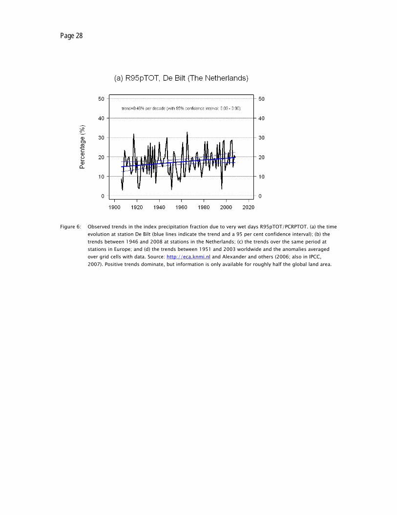
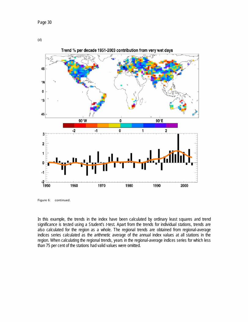
Figure 6 shows the calculated time evolution of R95pTOT/PRCPTOT for the Dutch station De Bilt together with the observed trends (1946-2008) for all available stations in the Netherlands and Europe. The majority of stations throughout Europe show significant positive trends, indicating a disproportionately large change in the extremes relative to the total amounts. The trend in the European average of the station specific index series in this period is 0.32 per cent per decade (with a 95 per cent confidence interval 0.14-0.51). This supports the notion of a relatively larger change of the extreme events compared with the annual amounts. Together with similar results for other regions of the world, this led IPCC (2007) to conclude that heavy precipitation events increased over most areas during the second half of the twentieth century, leading to a larger proportion of total rainfall in a year from heavy falls (Figure 6d).
Page 28
Figure 6: Observed trends in the index precipitation fraction due to very wet days R95pTOT/PCRPTOT. (a) the time evolution at station De Bilt (blue lines indicate the trend and a 95 per cent confidence interval); (b) the trends between 1946 and 2008 at stations in the Netherlands; (c) the trends over the same period at stations in Europe; and (d) the trends between 1951 and 2003 worldwide and the anomalies averaged over grid cells with data. Source: http://eca.knmi.nl and Alexander and others (2006; also in IPCC, 2007). Positive trends dominate, but information is only available for roughly half the global land area.

Page 29
(b)
(c)
Page 30
(d)
Figure 6: continued.
In this example, the trends in the index have been calculated by ordinary least squares and trend significance is tested using a Student’s t-test. Apart from the trends for individual stations, trends are also calculated for the region as a whole. The regional trends are obtained from regional-average indices series calculated as the arithmetic average of the annual index values at all stations in the region. When calculating the regional trends, years in the regional-average indices series for which less than 75 per cent of the stations had valid values were omitted.

Page 31
Linear trends are the simplest available indicators of changes in the climate, but simple trend analysis may not always detect underlying trends in local indices of extremes, particularly in indices of relatively rare events. Furthermore, the detection of a trend does not necessarily imply that the underlying cause of the change is known. Formal detection and attribution analysis that compares observations with model-simulated changes in extremes must determine whether observed trends are due to specific causes, such as external forcing on the climate system from rising greenhouse gas concentrations. Note that information about trends is useful when adaptation is concerned, even without a clear understanding of the causes of the trends. Because of relatively short observation records and/or large year-to-year variability, regional averaging is sometimes necessary to detect changes in extremes: spatial averaging reduces variability in the data series, making it easier for the signal to stand out.
4.2 Changes in rare extreme events
For more rare extremes, information on changes and non-stationarity can be obtained using extreme value theory. One can either calculate the extreme quantiles for different periods of time (both in the past and future) assuming that non-stationarity within the time periods is sufficiently small, or use more advanced methods in which the parameters in the statistical models vary over time to describe the temporal evolution of the extremes.
The extRemes toolkit introduced in Section 3.2 is able to incorporate a linear trend (or other covariate) into any of the three parameters of the GEV distribution. A likelihood ratio test can be performed to determine whether a model with a linear trend significantly improves the fit over a model that does not consider trend. An example of an analysis with the GEV distribution that allows for a linear trend in rare extremes will be presented at the end of this section.
As is the case with the indices, changes in rare extreme events may also be difficult to detect locally, even when powerful methods based on extreme value analysis theory are used. One approach that is sometimes used to meet this challenge is to make assumptions about how uncertain parameters in the extreme value distribution vary from one location to the next. For example, given that large-scale climatic influences may be more or less homogeneous in a given area, it may be appropriate to assume that the shape parameter in the GEV distribution has the same value at all locations. Similarly, in areas with homogeneous climate characteristics, it may be reasonable to assume that all parameters of the GEV distribution are homogeneous across the region, or that the scale and shape parameters are homogeneous.
Such an assumption would enable “data pooling” in which records from multiple stations are combined to form a larger data sample. The spatial pooling approach has its origin in hydrology where it is known as regional frequency analysis. This approach is most effective for variables, such as precipitation, which have short “decorrelation” distances (that is, where the correlation between observations at

Page 32
different locations falls off quickly as the distance between stations increases). Pooling can also be done in other ways, such as by averaging parameter estimates from nearby locations. Parameter estimates based on the pooled information across the region are generally less uncertain than those from the data of individual records because the same amount of information is used to estimate a smaller number of parameters. This also leads to a reduction of uncertainty of the estimated extreme quantiles of the distribution. As an example, Kharin and Zwiers (2000) pool information in an analysis of extremes simulated by global climate models by averaging GEV parameters from adjacent grid boxes. For precipitation extremes from regional climate model simulations, the index-flood procedure has been applied (Fowler and others, 2005; Hanel and others, 2009), which assumes that the shape parameter and the ratio of the scale-to-location parameters of the GEV distribution are constant over the region of interest. Other approaches could include more sophisticated spatial modelling, perhaps using Kriging or an objective analysis technique, of either the extreme value distribution parameter estimates or of estimated return values (Smith, R.L., pers. comm., 2009).
In addition to providing estimates of extreme quantiles or levels that are exceeded with a particular probability, methodologies using extreme value distributions such as the GEV distribution also allow for the examination of changes in the exceedance probability of events of a certain size. As noted previously, exceedance probabilities may be expressed in terms of changes in average waiting times between events of a fixed size, where the waiting time is given as 1/exceedance probability. For example, in a warming climate the early twentieth-century warm extremes that occurred with a probability of five per cent (or a waiting time of 20 years) will generally be exceeded more frequently under present-day conditions, as a result of which their waiting times will have decreased.
Examples
This first example is from Kharin and others (2007), who used extreme value theory to assess the projected changes in temperature and precipitation extremes in the ensemble of global climate models used in IPCC (2007). They calculated the 20-year return values of annual extremes of near-surface temperature and 24-h precipitation amounts for the late twentieth century (1981-2000) and then studied the changes in this quantile for the years 2046–65 and 2081–2100 under different emission scenarios.
Figure 7 shows the projected change in waiting times for events that occur on average once every 20 years under present climate conditions for the period 2046–2065 as simulated by global climate models. As illustrated in the figure, Kharin and others (2007) find that changes in the intensity of precipitation extremes are generally positive, even in subtropical regions where total precipitation generally decreases. This implies that waiting times are reduced in the future for late-twentieth-century extreme precipitation events as simulated by the climate models. The increase in precipitation extremes is consistent with the projected changes in more moderate extremes assessed using the descriptive indices.

Page 33
Figure 7: Box plots of waiting times for late-twentieth-century 20-year (24-hr) precipitation events as simulated by 14 IPCC models in 2046–65 with the SRES B1 (blue), A1B (green), and A2 (red) emission scenarios (Kharin and others, 2007). The boxes indicate the central 50 per cent inter-model range and the median. The whiskers extend to the lower and upper model extremes. The continent-wide regions and zonal bands considered are defined in the map. All regions show reductions in waiting times, indicating more intense precipitation extremes.

Page 34
The second example illustrates how the parameters in the statistical models may vary over time to reflect the temporal evolution of the extremes. It again makes use of the extRemes toolkit, now including a linear trend in the statistical model to analyze the change over time. As in Section 3.2, a GEV distribution is fitted to the highest one-day precipitation amounts in a year at station Gd. St. Bernhard (Switzerland), but with a linear trend in the location parameter. Note that trend can also be considered for the other two parameters as well. The likelihood ratio test indicates that the inclusion of a linear trend in the location parameter provides a significantly improved fit (at the five per cent significance level) to the observed extremes. Figure 8 shows a clear trend between 1901 and 2004.
The maximum likelihood estimates for the three parameters of the model with trend for Gd. St. Bernhard were found to be the following:
Parameter Gd. St. Bernhard
Location 41.58 + 0.46*(year-1900) (4.12, 0.07)
Scale 17.38 (1.51)
Shape -0.06 (0.09)
As in Section 3.2, inspection of the standard errors shown in parentheses reveals that the value for the shape parameter is well within its standard deviation from zero. Inclusion of a trend implies that no return-level plot can be provided because the expected extreme quantiles for each return period change over time. From the GEV model parameters, one can derive that the expected maximum daily precipitation at Gd. St. Bernhard exceeds some 82 mm on average every 20 years at the beginning of the observation series and some 141 mm on average every 20 years at the end of the series. Figure 8 shows that again a total of five data points exceed the 20-year return level (indicated by the green line) but these points are now evenly spread over time, indicating that the model with a linear trend in the location parameter is a clear improvement over the model without a trend used in Section 3.2.

Page 35
Figure 8: As Figure 4b, but now the green line for the 20-year return level has been estimated from the model which includes a linear trend in the location parameter of the GEV distribution.
Changes in extremes can also be assessed by using extreme value theory and calculating the extreme quantiles for different periods of time (both in the past and future) or by using more advanced methods in which the parameters in the statistical models vary over time to describe the temporal evolution of the extremes. The extRemes toolkit is able to incorporate a linear trend in time (or other covariate) in the analysis of extremes.

Page 36
5 Future extremes
5.1 Evidence of changes in extremes from observations
IPCC (2007) reports a number of observed changes in extremes over the past several decades based on instrumental series. In recent decades, most land areas of the world have experienced fewer cold days/nights (and frost days) and more hot days/nights (and heatwaves). Heavy precipitation events have increased over most areas, leading to a larger proportion of annual total rainfall from heavy falls. The few countries with sufficient data for reliable trend estimates, such as the United Kingdom and the United States of America, show increases in rare precipitation events (with return periods longer than 10 years) that are consistent with changes inferred for more robust statistics. The area affected by droughts has increased in many regions since 1970. Over the same period, the intensity and lifetime of tropical cyclones have increased in some regions, with no trend in frequency. The incidence of extreme high sea level (storm surges and extreme wave heights) has increased. Outside the tropics in the Northern Hemisphere, storm tracks have shifted northward and there is a net increase in storm frequency/intensity.
These changes reported by IPCC are partly based on the ETCCDI indices for moderate temperature and precipitation extremes. For example, the index R95pTOT representing the fraction of annual precipitation amount due to very wet days shows positive trends for the majority of stations (see Figure 6), indicating that heavy precipitation events increased over most areas sampled.
The evidence that humans are affecting the mean climate has become very strong and now includes aspects of the hydrological cycle. While these changes in the mean state will inevitably also affect the extremes of climate, it is likely that natural low-frequency climate fluctuations are also an important factor in observed changes in extremes. Our ability to discriminate between causes remains limited for many types of extremes because sufficiently long observation series are only available for a limited number of regions. Both the presence of natural low-frequency variability, which is in part associated with slow variation in the oceans and the cryosphere, and secular change caused by external influences, compromise the assumption of stationarity that is made in most extreme value analyses. Nevertheless, techniques that are able to cope with nonstationarity have begun to be applied to the analysis of climate and weather extremes.
For the moment, it remains difficult to detect significant changes in many types of extremes because of the limited amount of available observational information. This is because extreme events are rare by definition and because observational records, where available, are often not long enough. It should be noted that a failure to detect a significant trend indicates there is insufficient information to reliably identify change, but this does not necessarily mean that there is no change or that the likelihood of a given type of extreme event has not been affected by other changes that have been observed in the climate system. Thus, long-term monitoring of extremes is very important.

Page 37
The IPCC-AR4 reports a number of observed changes in extremes over the past decades based on instrumental series. These are partly based on the ETCCDI indices for moderate temperature and precipitation extremes. The detection of changes in extremes is difficult because they are rare, and thus the amount of information available for analysis is limited. Nevertheless, failure to detect changes in extremes at a given location does not mean that the frequency or intensity of extremes is not changing.
5.2 Evidence of changes in extremes from climate model projections
The model-projected changes in extremes reported by IPCC (2007) are in line with the observed changes over the past decades: fewer cold days/nights, more hot days/nights, a larger proportion of total rainfall from heavy falls, increasing drought area, increase in the incidence of extreme high sea level, and an increase in storm intensity in the Northern Hemisphere. The projected changes in temperature and precipitation extremes are partly based on the ETCCDI indices analysed for global climate model output as robust and unambiguous statistics for analyzing changes in moderate extremes.
It is important to note that large uncertainties and gaps in our knowledge of climate change and extremes remain. Climate model projections of changes in extremes are highly uncertain, in particular on adaptation-relevant regional and local scales (see for example Beniston and others, 2007). Nevertheless, climate models do provide qualitative information that can effectively be combined with estimates of current return values. For example, models project that current 20-year 24-hour precipitation events will have a return period of approximately 12–15 years (with broad uncertainty) by the middle of this century (Figure 7; Kharin and others, 2007). Should such a change occur, the probability of exceeding late-twentieth-century 20-year return levels would increase by approximately 33–66 per cent by mid-century. While climate models do not yet simulate precipitation extremes very reliably, the physical basis for intensifying extremes is understood.
The projected changes in extremes reported by IPCC (2007) are in line with the observed changes over the past decades. The projected changes in temperature and precipitation extremes are partly based on the ETCCDI indices analysed for global climate model output. It is important to note that large uncertainties and gaps in our knowledge of climate change remain, particularly concerning extremes on regional and local scales. Nevertheless, users should be informed of projected changes in extremes where the physical basis for change is understood, and where there is reasonable consensus amongst climate models.
Page 38
5.3 Information services on future extremes
The choice of the best approach for providing information services on changing weather and climate extremes depends on the specific application and the availability of resources. In general, the combined use of different techniques is recommended, as this will also provide information on the associated uncertainties.
If the statistical model fits the observed extremes well and there is no indication of change over time (as in the example for the daily rainfall maxima at station De Bilt in Section 3.2), then the estimated return levels that are obtained by assuming stationarity could continue to be used to inform the user about the probability that this event will happen in the relatively near future2. This advice would have to be combined with information regarding the effects of projected changes in climate (for example, as obtained from climate models) since, as has been noted, a lack of detection of change in an observed record should not be taken as an indication that a (currently weak) underlying signal is not present in the data. Given that there is already substantial evidence of human influence on the climate, there will inevitably be impacts on extremes in the future as the climate continues to warm. Consequently, the user should also be further advised to continue to closely monitor changes in extremes. On the other hand, if the observed extremes show a strong trend (as in the example for the daily rainfall maxima at station Gd. St. Bernhard in Section 4.2) or future climate model projections indicate that clear changes are likely to occur in the near-to-medium term, then users should be advised that current estimates of return levels based on assumptions of stationarity are likely to be inappropriate even for the near term.
Combining evidence of changes in extremes from observations and evidence of changes in extremes from climate model projections is possible by comparing the results of the different analysis techniques described in Sections 3 and 4. If the results for modest extremes and rarer extremes as well as the results using various analysis techniques all point in the same direction, more reliable climate services can be provided.
Continuing to work under the assumption that climate is stationary for the design criteria for (safety of) new infrastructure would disregard climate change. Climate change has already altered the mean, variability and extremes of relevant weather variables, and climate models project that these changes will continue. New infrastructure should be designed on the basis of both historical information on changes in extremes and projected future changes. The maximum value of a particular variable in the historical record can no longer be regarded as the normative value for design. Analogously, WMO recommends the use of operational normal values in addition to classic 30-year normal values for prediction (Trewin, 2007). Inclusion of climate model projected changes would even further improve the services, although the uncertainty of projected changes in local and regional extremes is high. It would be prudent to inform users of both current best estimates of return levels (taking non-stationarity into account if warranted by the statistical analysis) and of projected changes in the probability that these levels will be exceeded in coming years.
2 In this context, we think of “near term” as 1–2 decades, extending perhaps to 2020, and “medium term” as several decades, extending perhaps to 2040 or 2050.

Page 39
The choice of the best approach for providing information services on changing weather and climate extremes depends on the specific application and the availability of resources. In general, the combined use of different techniques is recommended, as this will also provide information on the uncertainties. Combining the evidence of changes in extremes from observations and climate model projections is possible by comparing the results of the different analyses techniques described in Section 4. New infrastructural works should be designed on the basis of both historical information on changes in extremes and projected future changes. Where necessary, the historical analysis should account for the effects of secular trends in the frequency and intensity of extremes in order to give the best estimate possible of current long-period return values.

Page 40
6 Measures to further improve our understanding
6.1 Data rescue, collection, digitization and sharing
NMHS services on weather and climate extremes depend critically on the availability of high-quality climate observations with sufficient spatial coverage over a long period of time. NMHSs have collected a large amount of historical station observations, but only a few have digitized their entire daily to sub-daily data holdings. Fewer still have homogenized their long time-series and made these generally available. New actions for Data Rescue (DARE) and digitization are necessary in many countries to improve availability and accessibility of historical climate data sets. WMO recommends standard practices and promotes knowledge on techniques, procedures and organizational matters of climate observations and data management (WMO, 2009). The Second Adequacy Report of the Global Climate Observing System (GCOS, 2003) developed the concept of Essential Climate Variables (ECVs) encompassing the atmospheric, oceanic and terrestrial domains. The concept forms part of the GCOS Implementation Plan (GCOS, 2004) and has been endorsed by the Group on Earth Observations (GEO) in its GEO System of Systems (GEOSS) work plan (GEO, 2007). Surface air temperature and precipitation are the prime ECVs for the atmospheric domain.
NMHS services on weather and climate extremes gain in quality if they are based on a thorough understanding and appreciation of the uncertainties and constraints associated with the use of both observational data and climate change projections based on regional and global models. This is more easily accomplished on a regional than national basis. The regional workshops organized by ETCCDI illustrate the benefits of working across national borders, as they involve participants from neighbouring countries as well as several well-qualified experts from around the world to provide guidance on the analysis of the climate data. When an internationally coordinated exact formula is used for each index, the analyses for one country fit together seamlessly with analyses in neighbouring countries. In turn, analyses are verified by means of similar results from neighbouring countries. The workshops help the regions to develop a robust regional capacity to meet national and regional needs for reliable climate information and to contribute to and participate in the global research and monitoring effort. The capacity-building aspect has helped foster a greater appreciation of the importance of long-term in situ daily data for analysis of climate variability and change.
The ETCCDI workshops help to reach GCOS goals for data preservation and exchange (GCOS, 2004). The series of derived indices are publicly available for almost all countries, enabling other scientists to undertake a variety of climate studies hitherto impossible, leading to more knowledge about climate change. Sharing the ETCCDI indices of extremes is a good step in the right direction, and the indices have already been of great use to scientists working on adaptation and climate model validation. Unfortunately, some NMHSs must charge for the acquisition of the underlying daily to sub-daily weather records, putting some data outside the integrated data sets of climate change information (in particular extremes). The success of IPCC assessments clearly indicates that climate science is advanced most effectively for the benefit of all users when knowledge and information are exchanged internationally and openly. Limiting accessibility undermines the generation of new knowledge about past climate change, potentially hindering the development of proper adaptation strategies. In fact, WMO requires a

Page 41
free exchange of data for the benefit of all countries. The covering letter for WMO Resolution 40 contains the statement that: “As a fundamental principle of the WMO, and in consonance with the expanding requirements for its scientific and technical expertise, WMO commits itself to broadening and enhancing the free and unrestricted exchange of meteorological and related data and products”.
The continued accumulation of basic climate data is vital forunderstanding past and current climate change, improving projections that are well constrained by past observed changes and developing strategies that ensure first and foremost that new infrastructure and systems are well adapted to current climate change. Climate monitoring is therefore absolutely necessary to provide important guidance as we navigate in the more uncertain world of climate change in near real time and attempt to adapt to those changes effectively, and in the most cost-effective manner.
NMHS services on weather and climate extremes depend critically on the availability of high-quality climate observations with sufficient spatial coverage over a long period of time. For many countries, new actions for Data Rescue (DARE) and digitization are necessary. Continued monitoring of climate is absolutely necessary for adaptation to climate change for all countries. Obtaining a thorough understanding and appreciation of the uncertainties and constraints associated with the use of both observational data and climate change projections based on global and regional models is more easily accomplished on a regional than national basis. The regional workshops organized by ETCCDI illustrate the benefits of working across national borders.
6.2 Climate change detection and attribution
There is increasing concern that weather and climate extremes may be changing in frequency and intensity as a result of human influences on climate. However, natural variability masks anthropogenic trends, creating uncertainty in attributing the causes of climate change. Extremes are, and always have been, part of natural climate variability. Single extreme events (such as the heatwave in Europe in the summer of 2003) cannot be simply and directly attributed to anthropogenic climate change if the event in question could have occurred naturally.
As noted by CCSP (2008), formal attribution studies have only recently been used to determine the causes of changes in some extremes at the scale of a continent. Certain aspects of observed increases in temperature extremes have been linked to human influences. The observed increase in heavy precipitation events is associated with an increase in water vapour, and the latter has been attributed to human-induced warming. There is evidence suggesting a human contribution to recent changes in hurricane activity as well as in storms outside the tropics, though a confident assessment will require further study (CCSP, 2008).
Improved data availability and knowledge of changes in extremes support the detection and attribution of anthropogenic influences on climate. Recent detection/attribution studies suggest that changes in extremes should be nearly as detectable (temperature) or even more detectable (precipitation) than
Page 42
changes in the mean (Hegerl and others, 2004). Progress in this discipline of climate change research means that scientists will be able to determine (at some pre-specified confidence level) the extent to which anthropogenic influence has increased the risk of a particular extreme event relative to the climate for the same period that would have occurred in the absence of human influence (Allen, 2003). Indeed, one recent study (Stott and others, 2004) estimated that anthropogenic influence likely increased the risk of a warm summer in Europe similar to that of 2003 during the 1990s by a factor of at least two compared to the climate that would have prevailed if only natural factors had been active.
Single extreme events cannot be simply and directly attributed to anthropogenic climate change if the event in question might have occurred naturally. However, there is evidence suggesting a human contribution to recent increases in some temperature and precipitation extremes at the scale of a continent. Improved data availability and knowledge of changes in extremes support the detection and attribution of anthropogenic influences on climate.

Page 43
7 Wider societal benefits
The Nairobi Work Programme (NWP) (UNFCCC, 2007), a five-year program (2005–2010) implemented by the Parties to the UNFCCC, aims at assisting countries, in particular developing countries, in improving their understanding and assessment of impacts, vulnerability and adaptation to climate change. Amongst the nine work areas of the NWP, one area is explicitly related to climate related risks and extreme events.
WMO, through its World Climate Programme (WCP), World Climate Research Programme (WCRP), Atmospheric Research and Environment Programme (AREP), GAW monitoring network (greenhouse gases and ozone) and Disaster Risk Reduction Programme (DRR), helps Members, in particular developing countries, to improve their understanding and assessment of impacts, vulnerability and adaptation. The goal is to make informed decisions on practical adaptation actions and to base measures to respond to climate change on a sound, scientific, technical and socio-economic foundation, taking into account current and future climate change and variability (WMO, 2007b). WMO proposes to establish a new Global Framework for Climate Services (GFCS) with the goal to “enable climate adaptation and climate risk management through the incorporation of science-based climate information and prediction into policy and practice at all levels.”
The content of this guidelines document and the results of the extremes analyses that it describes will support climate-policy-related research at the local, national and regional scales and will provide WMO Members and NMHSs with practical information in developing new high-level decision-making and policy types of climate information. Local authorities and national decision-makers will be able to utilize the extremes analyses for their country or region as input for climate change assessments and the formulation of adaptation and mitigation strategies. It is information on the longer multi-decadal time scale that is needed for governments to minimize and adapt to the societal and environmental impacts of climate variability and change. For adaptation planning, the longer (multi-decadal) time scales are particularly relevant, because nearly all infrastructure design relies on assessment of probabilities of extremes with return periods of 20 years or more.
Individual countries can directly use the results for their “national communications on climate change policies”, which are a written requirement for the Conference of the Parties of UNFCCC and include national GCOS implementation activities.

Page 44
An additional benefit of extremes analysis is that it encourages countries to improve their observing systems. Regarding the future, the introduction of unwanted non-climatic changes is better avoided altogether. Guidance on managing change in observational programmes in a manner that best maintains the required integrity of the climate record is provided in Street and others (2007).
The results of the extremes analyses described in this document will support climate-policy-related research at the local and national scales. Local authorities and national decision-makers will be able to utilize the extremes analyses for their country as input for climate change assessments and the formulation of adaptation and mitigation strategies. Countries can also directly use the results for their “national communications on climate change policies”, which are a written requirement for the Conference of the Parties of UNFCCC and include national GCOS implementation activities.

Page 45
References Aguilar, E., I. Auer, M. Brunet, T.C. Peterson and J. Wieringa, 2003: Guidelines on climate metadata and homogenization.
WCDMP No. 53 – WMO/TD-No. 1186.
Alexander, L.V., X. Zhang, T.C. Peterson, J. Caesar, B. Gleason, A.M.G. Klein Tank, M. Haylock, D. Collins, B. Trewin, F. Rahimzadeh, A. Tagipour, P. Ambenje, K. Rupa Kumar, J. Revadekar and G. Griffiths, 2006: Global observed changes in daily climate extremes of temperature and precipitation. J. Geophys. Res., 111 (D05109), DOI:10.1029/2005JD006290.
Allen, M., 2003: Liability for climate change. Nature, 421, 891–892. Barnett, T.P., D.W. Pierce, H.G. Hidalgo, C. Bonfils, B.D. Santer, T. Das, G. Bala, A.W. Wood, T. Nozawa, A.A. Mirin, D.R.
Cayan and M.D. Dettinger, 2008: Human-induced changes in the hydrology of the Western United States, Science, 319, 1080–1083, DOI:10.1126/science.1152538.
Beniston, M., D.B. Stephenson, O.B. Christensen, C.A.T. Ferro, C. Frei, S. Goyette, K. Halsnaes, T. Holt, K. Jylhä, B. Koffi, J. Palutikof, R. Schöll, T. Semmler and K. Woth, 2007:. Future extreme events in European climate: an exploration of regional climate model projections. Climatic Change, DOI:10.1007/s10584–006-9226-z.
Brandsma, T. 2001: Weather type dependent homogenization of the daily Zwanenburg/De Bilt temperature series. In: S. Szalai (ed.). Proceedings of the Third Seminar for Homogenization and Quality Control in Climatological Databases, Budapest, Hungary, 25–29 September 2000.
Brink, H.W. van den and G.P. Können, 2008: The statistical distribution of meteorological outliers. Geophys. Res. Lett., DOI:10.129/2008GL035967.
Brinke, W.B.M. ten, B.A. Bannink and W. Ligtvoet, 2008: The evaluation of flood risk policy in the Netherlands. Water Management, 161, 181–188, DOI: 10.1680/wama.2008.161.4.181.
Brunet, M., O. Saladié, P. Jones, J. Sigró, E. Aguilar, A. Moberg, D.Lister, A. Walther and C. Almarza, 2008. A case study/guidance on the development of long-term daily adjusted temperature datasets. WCDMP No. 66 – WMO/TD-No. 1425.
Buishand, T.A., G.T. Kempen, A.J. Frantzen, H.F.R. Reijnders and A.J. van den Eshof, 1988: Trend and seasonal variation of precipitation chemistry data in the Netherlands. Atmospheric Environment, 22, 339–348.
CCSP, 2008: Weather and Climate Extremes in a Changing Climate. Regions of Focus: North America, Hawaii, Caribbean, and U.S. Pacific Islands. A Report by the U.S. Climate Change Science Program and the Subcommittee on Global Change Research. [Thomas R. Karl, Gerald A. Meehl, Christopher D. Miller, Susan J. Hassol, Anne M. Waple and William L. Murray (eds.)]. Department of Commerce, NOAA’s National Climatic Data Center, Washington, D.C., USA, 164 pp. Available from http://www.climatescience.gov/Library/sap/sap3-3/final-report/sap3-3-final-all.pdf
Cleveland, W.S., 1979: Robust locally weighted regression and smoothing scatterplots, J. Am. Stat. Assoc., 74, 829–836.
Coles, S.G., 2001a: An Introduction to Statistical Modeling of Extreme Values, Springer-Verlag, London. Coles, S.G., 2001b: S-plus functions for extreme value modeling: An accompaniment to the book An Introduction to
Statistical Modeling of Extreme Values. http://www.stats.bris.ac.uk/ masgc/ismev/uses.ps
Cornford, S.G., 2003: Socio-economic impacts of weather events in 2002. WMO Bulletin, 52, 269–290.
Della-Marta, P.M., H. Wanner, 2006: A method of homogenizing the extremes and mean of daily temperature measurements. Journal of Climate, 19, 4179–4197.
Dupuis, D.J. and M. Tsao, 1998: A hybrid estimator for the Generalized Pareto and Extreme-Value Distributions. Communications in Statistics: Theory and Methods, 27, 925–941.

Page 46
Fowler, H.J., M. Ekström, C.G. Kilsby and P.D. Jones, 2005: New estimates of future changes in extreme rainfall across the UK using regional climate model integrations, 1. Assessment of control climate, J. Hydrol., 300, 212–233, DOI:10.1016/j.jhydrol.2004.06.017.
Frei, C. and C. Schär, 2001: Detection probability of trends in rare events: theory and application to heavy precipitation in the Alpine region. Journal of Climate, 14, 1568–1584.
GCOS, 2003: GCOS Second Report on the Adequacy of the Global Climate Observing System in Support of the UNFCC. GCOS-92, WMO/TD-No. 1143, 75 pp.
GCOS, 2004: GCOS Implementation Plan for Global Observing System for Climate in support of UNFCC. GCOS-92, WMO/TD-No. 1219, 136 pp.
GEO, 2007: GEO Group on Earth Observations Work Plan for 2007–2009. March 2007. 37 pp., www.earthobservations.org/documents/wp0709_v4.pdf
Gilleland, E. and Katz R.W., 2005: Tutorial for the Extremes Toolkit: Weather and Climate Applications of Extreme Value Statistics, http://www.assessment.ucar.edu/toolkit
Gilleland, E. and Katz, R.W., 2006: Analyzing seasonal to interannual extreme weather and climate variability with the Extremes Toolkit (extRemes). Preprints: 18th Conference on Climate Variability and Change, 86th American Meteorological Society (AMS) Annual Meeting, 29 January–2 February 2006, Atlanta, Georgia. P2.15
Giorgi, F., 2008: Regionalization of climate change information for impact assessment and adaptation. WMO Bulletin, 57 (2), 86–92.
Groisman, P.Y., T.R. Karl, D.R. Easterling, R.W. Knight, P.F. Jamason, K.J. Hennessy, R. Suppiah, C.M. Page, J. Wibig, K. Fortuniak, V.N. Razuvaev, A. Douglas, E. Forland and P-M. Zhai, 1999: Changes in the probability of heavy precipitation: important indicators of climatic change. Climatic Change, 43, 243–283.
Gumbel, E.J., 1958: Statistics of Extremes. Columbia University Press, New York, 375pp.
Hanel, M., T.A. Buishand and C.A.T. Ferro, 2009: A non-stationary index-flood model for precipitation extremes in transient regional climate model simulations. J. Geophys. Res., in press.
Haylock, M.R., N. Hofstra, A.M.G. Klein Tank, E.J. Klok, P.D. Jones and M. New, 2008: A European daily high-resolution gridded dataset of surface temperature and precipitation. J. Geophys. Res., 113, DOI:10.1029/2008JD10201.
Hegerl, G.C., F. Zwiers, P. Stott and S. Kharin, 2004: Detectability of anthropogenic changes in annual temperature and precipitation extremes. Journal of Climate, 17, 3683–3700.
Hosking, J.R.M., 1990: L-moments: Analysis and estimation of distributions using linear combinations of order statistics. J. Roy. Stat. Soc. (Ser. A), B52, 105–124.
Houghton, J.T., Y. Ding, D.J. Griggs, M. Noguer, P.J van der Linden and D. Xiaosu (eds.), 2001. Climate Change 2001: The Scientific Basis. Contribution of Working Group I to the Third Assessment Report of the Intergovernmental Panel on Climate Change (IPCC). Cambridge University Press, UK, pp944.
IPCC, 2007: Climate Change 2007: The Physical Science Basis. Contribution of Working Group I to the Fourth Assessment Report of the Intergovernmental Panel on Climate Change [Solomon, S., D. Qin, M. Manning, Z. Chen, M. Marquis, K.B. Averyt, M.Tignor and H.L. Miller (eds.)]. Cambridge University Press, Cambridge, United Kingdom and New York, NY, USA, 996 pp.
Jenkinson, A. F., 1955: The frequency distribution of the annual maximum (or minimum) values of meteorological elements. Quart. J. Roy. Meteor. Soc., 81, 158–171.
Katz, R.W., M.B. Parlange and P. Naveau, 2002: Statistics of extremes in hydrology, Advances in Water Resources, 25, 1287–1304.
Kendall, M. G., 1938: A new measure of rank correlation. Biometrika, 30, 81–93.

Page 47
Kharin, V.V. and F.W. Zwiers, 2000: Changes in the extremes in an ensemble of transient climate simulations with a coupled atmosphere–ocean GCM. Journan of Climate, 13, 3760–3788.
Kharin, V.V. and F.W. Zwiers, 2005: Estimating extremes in transient climate change simulations. Journal of Climate, 18, 1156–1173.
Kharin, V.V., F.W. Zwiers, X. Zhang and G.C. Hegerl, 2007: Changes in temperature and precipitation extremes in the IPCC ensemble of global coupled model simulations. Journal of Climate, 20, 1419-1444, DOI: 10.1175/JCLI4066.1
Klein Tank, A.M.G. and G.P. Können, 2003: Trends in indices of daily temperature and precipitation extremes in Europe, 1946–99. Journal of Climate, 16, 3665–3680.
Landwehr, J.M., N.C. Matalas and J.M. Wallis, 1979: Probability weighted moments compared with some traditional techniques in estimating Gumbel parameters and quantiles. Water Res. Research, 15, 1055–1064.
Milly, P.C.D., J. Betancourt, M. Falkenmark, R.M. Hirsch, Z.W. Kundzewicz, D.P. Lettenmaier and R.J. Stouffer, 2008: Stationarity is dead: whither water management? Science, 319, 573–574.
Min, S.-K., X. Zhang and F. Zwiers, 2008: Human-induced Arctic moistening. Science, 320, 518–520, DOI:10.1126/science.1153468.
Peterson, T.C. and M.J. Manton, 2008: Monitoring changes in climate extremes – A tale of international collaboration. BAMS, DOI:10.1175/2008BAMS2501.1.
Smith, R.L., 2002: Statistics of extremes with applications in environment, insurance and finance. http://www.stat.unc.edu/postscript/rs/semstatrls.pdf
Smith, R.L., 2008: Statistical Trend Analysis, in Weather and Climate Extremes in a Changing Climate. Regions of Focus: North America, Hawaii, Caribbean, and U.S. Pacific Islands. T.R. Karl, G.A. Meehl, C.D. Miller, S.J. Hassol, A.M. Waple, and W.L. Murray, editors. A Report by the U.S. Climate Change Science Program and the Subcommittee on Global Change Research, Washington, DC. Available from http://www.climatescience.gov/Library/sap/sap3-3/final-report/sap3-3-final-all.pdf
Stephenson, A. and E. Gilleland, 2006: Software for the analysis of extreme events: the current state and future directions. Extremes 8, 87–109.
Stott, P.A., D.A. Stone, and M.R. Allen, 2004: Human contribution to the European heatwave of 2003. Nature, 432, 610–614.
Street, R.B., D. Allsopp and Y. Durocher, 2007: Guidelines for managing changes in climate observation programmes. WMO/TD-No. 1378.
Trewin, B., 2007: The role of climatological normals in a changing climate. WCDMP No. 61 – WMO/TD-No. 1377.
UNFCCC, 2007: The NAIROBI WORK PROGRAMME on Impacts, Vulnerability and Adaptation to Climate Change. http://unfccc.int/files/adaptation/sbsta_agenda_item_adaptation/application/pdf/ nwp_brochure.pdf
Vincent, L.A., X. Zhang, B.R. Bonsal and W.D. Hogg, 2002: Homogenization of daily temperatures over Canada. Journal of Climate, 15, 1322–1334.
Wang, X.L., Q.H. Wen and Y. Wu., 2007: Penalized Maximal t-test for Detecting Undocumented Mean Change in Climate Data Series. J. App. Meteor. Climatol., 46, 916–931.
Wang, X.L., 2008a: Accounting for autocorrelation in detecting mean-shifts in climate data series using the penalized maximal t or F test, J. Appl. Meteorol. Climatol, 47, 2423-2444. DOI:10.1175/2008JAMC1741.1
Wang, X.L., 2008b: Penalized maximal F test for detecting undocumented mean shift without trend change, J. Atmos. Ocean. Technol., 25, 368–384.
Wijngaard, J.B., A.M.G. Klein Tank and G.P. Können, 2003: Homogeneity of 20th century European daily temperature and precipitation series. Int. J. Climatol., 23, 679–692.

Page 48
WMO, 1983: Guide to Climatological Practices, Second edition. WMO-No. 100. Now being updated: Third Edition working draft 3 May 2007 available from: http://www.wmo.int/pages/prog/wcp/ccl/ guide/guide_climat_practices.html
WMO, 1989: Statistical Distributions for Flood Frequency Analysis. WMO-No. 718 and Operational Hydrology Report No. 33.
WMO, 2007a: Climate information for adaptation and development needs. WMO-No. 1025. WMO, 2007b: Fifteenth World Meteorological Congress, Abridged final report with resolutions.
WMO-No. 1026.
WMO, 2009: Climate Observations and Climate Data Management Guidelines. WCDMP No. 68 – WMO/TD-No. 1481.
Wilks, D.S., 1995: Statistical Methods in the Atmospheric Sciences, second edition. International Geophysics Series, Vol. 59, Academic Press, 464pp.
Zhai, P. (ed.), 2005: Guidelines on Climate Watches. WCDMP No. 62 – WMO/TD-No. 1378.
Zhang, X., G. Hegerl, F.W. Zwiers and J. Kenyon, 2005: Avoiding inhomogeneity in percentile-based indices of temperature extremes, J. Clim., 18, 1641–1651.
Zhang, X., F.W. Zwiers, G.C. Hegerl, F.H. Lambert, N.P. Gillett, S. Solomon, P.A. Stott and T. Nozawa, 2007: Detection of human influence on twentieth-century precipitation trends. Nature, DOI:10.1038/nature06025.
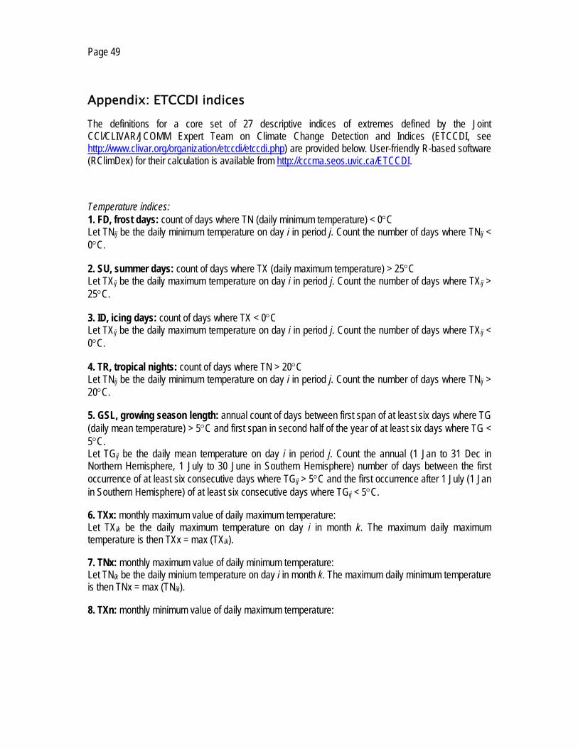
Page 49
Appendix: ETCCDI indices
The definitions for a core set of 27 descriptive indices of extremes defined by the Joint CCl/CLIVAR/JCOMM Expert Team on Climate Change Detection and Indices (ETCCDI, see http://www.clivar.org/organization/etccdi/etccdi.php) are provided below. User-friendly R-based software (RClimDex) for their calculation is available from http://cccma.seos.uvic.ca/ETCCDI.
Temperature indices: 1. FD, frost days: count of days where TN (daily minimum temperature) < 0°C Let TNij be the daily minimum temperature on day i in period j. Count the number of days where TNij < 0°C.
2. SU, summer days: count of days where TX (daily maximum temperature) > 25°C Let TXij be the daily maximum temperature on day i in period j. Count the number of days where TXij > 25°C.
3. ID, icing days: count of days where TX < 0°C Let TXij be the daily maximum temperature on day i in period j. Count the number of days where TXij < 0°C.
4. TR, tropical nights: count of days where TN > 20°C Let TNij be the daily minimum temperature on day i in period j. Count the number of days where TNij > 20°C.
5. GSL, growing season length: annual count of days between first span of at least six days where TG (daily mean temperature) > 5°C and first span in second half of the year of at least six days where TG < 5°C. Let TGij be the daily mean temperature on day i in period j. Count the annual (1 Jan to 31 Dec in Northern Hemisphere, 1 July to 30 June in Southern Hemisphere) number of days between the first occurrence of at least six consecutive days where TGij > 5°C and the first occurrence after 1 July (1 Jan in Southern Hemisphere) of at least six consecutive days where TGij < 5°C.
6. TXx: monthly maximum value of daily maximum temperature: Let TXik be the daily maximum temperature on day i in month k. The maximum daily maximum temperature is then TXx = max (TXik).
7. TNx: monthly maximum value of daily minimum temperature: Let TNik be the daily minium temperature on day i in month k. The maximum daily minimum temperature is then TNx = max (TNik).
8. TXn: monthly minimum value of daily maximum temperature:

Page 50
Let TXik be the daily maximum temperature on day i in month k. The minimum daily maximum temperature is then TXn = min (TXik).
9. TNn: monthly minimum value of daily minimum temperature: Let TNik be the daily minimum temperature on day i in month k. The minimum daily minimum temperature is then TNn = min (TNik).
10. TN10p, cold nights: count of days where TN < 10th percentile Let TNij be the daily minimum temperature on day i in period j and let TNin10 be the calendar day 10th percentile of daily minimum temperature calculated for a five-day window centred on each calendar day in the base period n (1961-1990). Count the number of days where TNij < TNin10.
11. TX10p, cold day-times: count of days where TX < 10th percentile Let TXij be the daily maximum temperature on day i in period j and let TXin10 be the calendar day 10th percentile of daily maximum temperature calculated for a five-day window centred on each calendar day in the base period n (1961-1990). Count the number of days where TXij < TXin10.
12. TN90p, warm nights: count of days where TN > 90th percentile Let TNij be the daily minimum temperature on day i in period j and let TNin90 be the calendar day 90th percentile of daily minimum temperature calculated for a five-day window centred on each calendar day in the base period n (1961-1990). Count the number of days where TNij > TNin90.
13. TX90p, warm day-times: count of days where TX > 90th percentile Let TXij be the daily maximum temperature on day i in period j and let TXin90 be the calendar day 90th percentile of daily maximum temperature calculated for a five-day window centred on each calendar day in the base period n (1961-1990). Count the number of days where TXij > TXin90.
14. WSDI, warm spell duration index: count of days in a span of at least six days where TX > 90th percentile Let TXij be the daily maximum temperature on day i in period j and let TXin90 be the calendar day 90th percentile of daily maximum temperature calculated for a five-day window centred on each calendar day in the base period n (1961-1990). Count the number of days where, in intervals of at least six consecutive days TXij > TXin90.
15. CSDI, cold spell duration index: count of days in a span of at least six days where TN > 10th percentile Let TNij be the daily minimum temperature on day i in period j and let TNin10 be the calendar day 10th percentile of daily minimum temperature calculated for a five-day window centred on each calendar day in the base period n (1961-1990). Count the number of days where, in intervals of at least six consecutive days TNij < TNin10.
16. DTR, diurnal temperature range: mean difference between TX and TN (°C) Let TXij and TNij be the daily maximum and minium temperature on day i in period j. If I represents the total number of days in j then the mean diurnal temperature range in period j DTRj = sum (TXij - TNij) / I.

Page 51
Precipitation indices: 17. RX1day, maximum one-day precipitation: highest precipitation amount in one-day period Let RRij be the daily precipitation amount on day i in period j. The maximum one-day value for period j is RX1dayj = max (RRij).
18. RX5day, maximum five-day precipitation: highest precipitation amount in five-day period Let RRkj be the precipitation amount for the five-day interval k in period j, where k is defined by the last day. The maximum five-day values for period j are RX5dayj = max (RRkj).
19. SDII, simple daily intensity index: mean precipitation amount on a wet day Let RRij be the daily precipitation amount on wet day w (RR ≥ 1 mm) in period j. If W represents the number of wet days in j then the simple precipitation intensity index SDIIj = sum (RRwj) / W.
20. R10mm, heavy precipitation days: count of days where RR (daily precipitation amount) ≥ 10 mm Let RRij be the daily precipitation amount on day i in period j. Count the number of days where RRij ≥ 10 mm.
21. R20mm, very heavy precipitation days: count of days where RR ≥ 20 mm Let RRij be the daily precipitation amount on day i in period j. Count the number of days where RRij ≥ 20 mm.
22. Rnnmm: count of days where RR ≥ user-defined threshold in mm Let RRij be the daily precipitation amount on day i in period j. Count the number of days where RRij ≥ nn mm.
23. CDD, consecutive dry days: maximum length of dry spell (RR < 1 mm) Let RRij be the daily precipitation amount on day i in period j. Count the largest number of consecutive days where RRij < 1 mm.
24. CWD, consecutive wet days: maximum length of wet spell (RR ≥ 1 mm) Let RRij be the daily precipitation amount on day i in period j. Count the largest number of consecutive days where RRij ≥ 1 mm.
25. R95pTOT: precipitation due to very wet days (> 95th percentile) Let RRwj be the daily precipitation amount on a wet day w (RR ≥ 1 mm) in period j and let RRwn95 be the 95th percentile of precipitation on wet days in the base period n (1961-1990). Then R95pTOTj = sum (RRwj), where RRwj > RRwn95.
26. R99pTOT: precipitation due to extremely wet days (> 99th percentile)

Page 52
Let RRwj be the daily precipitation amount on a wet day w (RR ≥ 1 mm) in period j and let RRwn99 be the 99th percentile of precipitation on wet days in the base period n (1961-1990). Then R99pTOTj = sum (RRwj), where RRwj > RRwn99.
27. PRCPTOT: total precipitation in wet days (> 1 mm) Let RRwj be the daily precipitation amount on a wet day w (RR ≥ 1 mm) in period j. Then PRCPTOTj = sum (RRwj).

For more information, please contact:
World Meteorological Organization
Observing and Information Systems DepartmentTel.: +41 (0) 22 730 82 68 – Fax: +41 (0) 22 730 80 21
E-mail: [email protected]
7 bis, avenue de la Paix – P.O. Box 2300 – CH 1211 Geneva 2 – Switzerland
www.wmo.int
Guidelines on Analysis of extremes in a changing climate in support of informed decisions for adaptation
Climate Data and Monitoring WCDMP-No. 72
WMO-TD No. 1500