Towson UniversityDepartment of Economics

Working Paper Series

Working Paper No. 2020-02

Health Risk and the WelfareEffects of Social Security

By Shantanu Bagchi and Juergen Jung

October 2021

© 2020 by Author. All rights reserved. Short sections of text, not to exceed twoparagraphs, may be quoted without explicit permission provided that full credit, including© notice, is given to the source.

Health Risk and the Welfare Effects of SocialSecurity∗

Shantanu Bagchi†

Towson UniversityJuergen Jung‡

Towson University

October 12, 2021

Abstract

We quantify the importance of idiosyncratic health risk in a calibrated general-equilibriummodel of Social Security. We construct an overlapping-generations model with rational-expectationshouseholds, idiosyncratic labor income and health risk, profit-maximizing firms, incomplete in-surance markets, and a government that provides pensions and health insurance. We calibratethis model to the U.S. economy and perform two sets of computational experiments: (i) wedecrease the size of Social Security, and (ii) we modify the progressivity of Social Security’sbenefit-earnings rule. We find that cutting Social Security’s payroll tax in general equilibriumincreases overall welfare, but by a lesser extent when health risk is present. When we modify theprogressivity of Social Security’s benefit-earnings rule, we find that a lump-sum benefit unrelatedto past income increases overall welfare, but by a larger extent in the presence of health risk.A linear (fully proportional) benefit-earnings rule, on the other hand, reduces overall welfare,but also by a larger extent in the presence of health risk. Together, our results suggest thatSocial Security’s implicit insurance is more valuable for low- and medium-income householdswhen health risk is present in the model environment.

JEL: E62, E21, H31, H55, I14Keywords: Health risk, Social Security, benefit-earnings rule, consumption smoothing, generalequilibrium.

∗We thank Matt Chambers, Svetlana Pashchenko, Ponpoje Porapakkarm, Kai Zhao, participants of the CBE D&RConference at Towson University in 2019, participants of the Midwest Macro Meetings 2019, and participants of theIIPF Annual Congress 2019.Declaration of Interest:Dr. Bagchi received a Summer Research Grant from the College of Business and Economics at Towson University.Beyond that he has no further relevant or material financial interests that relate to the research described in thispaper.Dr. Jung has no relevant or material financial interests that relate to the research described in this paper.

†Department of Economics, Towson University, U.S.A., E-mail: sbagchi@towson.edu‡Department of Economics, Towson University, U.S.A., E-mail: jjung@towson.edu

1

1 Introduction

While the primary justification for the creation of Social Security in 1935 was to create “moreadequate provision for aged persons,”1 today it accounts for 16–17 percent of total annual federalgovernment expenditures, second only to health expenditures (excluding defense). Economists havetraditionally viewed Social Security as a vehicle that partially insures individuals against risks thatmarkets do not insure well, such as the risk of an uncertain lifetime, and the risk of unfavorablelabor-market outcomes causing old-age poverty. Social Security annuities are paid until death, sothey are commonly believed to insure individuals against the risk of out-living their own savings.Meanwhile, Social Security benefits are a concave function of work-life earnings, and this concavityis intended to enable better work-retirement consumption smoothing, particularly when events suchas unemployment and economic recessions negatively impact early-life labor income.

While public pension programs, in general, are understood to have important insurance effects,there is also considerable evidence that such programs negatively affect households’ consumption,saving, and labor supply decisions. In particular, Social Security causes households to exit fromthe labor market earlier, to work fewer hours during employment, and to also reduce the personalsavings needed for financing retirement consumption (Jeske, 2003; Wallenius, 2013; Alonso-Ortiz,2014). Therefore the literature on Social Security’s overall welfare consequences has traditionallyevolved as a comparison of the benefits of its insurance effects, to its distortionary costs on householdbehavior. This literature has broadly concluded that under traditional preferences, the welfare gainsfrom the insurance effects of Social Security are usually smaller than its distortionary welfare losses(Auerbach and Kotlikoff, 1987; Bagchi, 2015), although some find overall welfare gains, especiallywhen labor supply is inelastic (Hubbard and Judd, 1987; İmrohoroğlu, İmrohoroğlu and Joines,1995). This literature, however, has typically ignored how Social Security might interact with athird type of risk: the risk related to one’s health status.

On the one hand, Social Security transfers resources from early life, when health risks are rel-atively low, to old age, when health risks are considerably higher. This transfer can potentiallyimprove welfare, especially if households cannot save efficiently for uncertain old-age medical ex-penditures. While there are both public and private avenues that allow households to partiallyinsure against health risks, such as Medicaid, Medicare, employment-based health insurance, andindividual health insurance, the impact of Social Security on consumption-smoothing in the contextof health risk is not well understood. On the other hand, as households engage in precautionarysavings due to the presence of health risk in their budget constraints, Social Security has a negativeeffect on disposable income in early life, especially for households that are borrowing constrained,which can distort precautionary savings and potentially reduce welfare. Traditional welfare analysesof Social Security have typically abstracted from health risks, and have therefore overlooked thesemechanisms (e.g., Hubbard and Judd, 1987; İmrohoroğlu, İmrohoroğlu and Joines, 1995; Bagchi,2015).

In this paper, we quantify the importance of idiosyncratic health risk in a calibrated generalequilibrium model of Social Security. More specifically, we compare the welfare implications of

1The legislative history of the Social Security Act of 1935 is available on http://www.ssa.gov/history.

2

Social Security in an environment with labor income, mortality, as well as health risks, to those inan environment where health risk is removed from the model. To do this, we begin by constructinga calibrated general-equilibrium macroeconomic model with households, firms, markets for goodsand services, and a government that provides partial insurance against income and health risks.Then, we compute two experiments with this model. First, in order to assess the overall welfareeffects of Social Security in our model environment, we cut its payroll tax rate by 50 percent fromits current level. Second, to evaluate how the degree of redistribution implicit in Social Securityaffects households with varying degrees of economic resources, we modify the progressivity of SocialSecurity’s benefit-earnings rule. To tease out the precise effect of health risk, we repeat theseexperiments in a hypothetical version of our model in which we completely remove health risk froma household’s economic environment. We also examine the implications of these experiments forlabor supply, consumption, and saving decisions, the markets for goods and services, the values ofkey macroeconomic aggregates, and the government’s budget.

In general, our findings indicate that health risk has important implications for the welfare ef-fects of Social Security. The presence of partially insured health risk, especially in old age, increasesthe long-term consumption smoothing benefits of Social Security, but its payroll tax reduces dis-posable income in early life, and negatively affects short-term consumption smoothing by reducinga household’s ability to self-insure against such risk. We find that in our model framework, down-sizing Social Security leads to higher welfare in general equilibrium, but the welfare gain is smallerwhen we account for health risk. Similarly, modifying the progressivity of the benefit-earnings rule,we find that with health risk, increased progressivity has a larger positive effect on overall welfare,and reduced progressivity has a larger negative effect. In other words, our results suggest thatignoring the effect of health risk on labor income, household expenditures, and survivorship in ageneral-equilibrium environment underestimates the insurance value of Social Security in our model.

Given that the key mechanism in our model is the trade-off between long- and short-term con-sumption smoothing, we examine how our computational results change with respect to a house-hold’s coefficient of relative risk aversion: the parameter that controls the strength of the precau-tionary motive. We find that as expected, when risk aversion is high, the precautionary motive isstronger in the benchmark economy, so Social Security’s welfare consequences are largely unaffectedby whether or not heath risk is present in the model environment. On the other hand, when riskaversion is low, the precautionary motive is weaker in the benchmark economy, so health risk mat-ters more for the welfare consequences. In fact, in this case the response to the presence of healthrisk is so large that households experience a larger welfare gain from downsizing Social Security inthe environment with health risk.

The U.S. experienced a significant regulatory overhaul of its healthcare system almost a decadeago. On March 23, 2010, President Barack Obama signed into law the Patient Protection andAffordable Care Act, also known as the ACA, as the largest piece of healthcare reform legislationin the U.S. over the past 40 years. While there is a burgeoning literature that examines theimplications of the ACA with respect to household-level healthcare spending and welfare, not muchis known regarding the role of Social Security in providing insurance against health risks. Currently,

3

economists and policymakers understand Social Security as providing insurance against income andmortality risks, and the literature has already shown that under traditional preferences, these effectsmay not be strong enough to yield overall welfare gains. However, insurance against health risksprovides two separate channels through which Social Security might affect welfare: (i) the self-insurance channel and (ii) the redistribution of health risk channel. To the best of our knowledge,our paper is the first to quantitatively evaluate and compare the importance of these two channels.

The remainder of the paper is structured as follows. Section 2 briefly reviews the literature.Section 3 introduces the computational model. Section 4 outlines our baseline calibration. Wediscuss our computational experiments and their results in Section 5. Finally, we conclude inSection 6.2

2 Related literature

As discussed in Glomm and Jung (2013), government transfers can be classified as early (i.e.,transfers to the young) vs. late (i.e., transfers to the old). Both transfers are associated with acertain level of tax distortions that the government can attempt to minimize. In this project, ourobjective is to examine the effects of health risk on the welfare implications of a late redistributionsystem—U.S. Social Security—focusing either on the revenue or the spending side. We do this inan environment with realistic mortality, labor income, and health risks, where health risk affectshousehold income, medical expenditures, and survivorship. This research contributes to severalrelated strands of the literature.

First, starting with Abel (1985) and Hubbard and Judd (1987), a number of studies haveexamined the importance of the traditional roles of unfunded public pensions in justifying thesize of U.S. Social Security. Abel (1985) and Hubbard and Judd (1987) find a welfare-improvingrole for Social Security in a model with mortality risk and closed annuity markets, but Hubbardand Judd (1987) find that these welfare gains are significantly reduced or even eliminated whenborrowing constraints are introduced. In a related study, İmrohoroğlu, İmrohoroğlu and Joines(1995) examine the optimality of Social Security in a life-cycle economy with mortality risk, missingannuity markets, idiosyncratic employment risk, and borrowing constraints. While this literaturedoes not arrive at a consensus regarding the optimal size of Social Security in the U.S., it generallyconcludes that the welfare-improving role of Social Security is much smaller once the consumption,saving, and labor supply distortions from Social Security are accounted for. Our analysis extendsthis literature by comprehensively accounting for health risk in a household’s budget constraint aswell as the utility function, all within a calibrated general equilibrium model of Social Security.

Second, there are a number of studies that jointly examine Social Security and health riskin their model frameworks. For example, İmrohoroğlu and Kitao (2012) evaluate Social Securityreform proposals accounting for benefit claiming and labor force participation using a general-equilibrium model with health risk, and Braun, Kopecky and Koreshkova (2017) evaluate the welfareimplications of means tested social insurance, such as Medicaid and Supplemental Security Income,

2Appendices A–B present additional information about the data used for estimating the income profiles and healthtransition probabilities.

4

conditional on current U.S. Social Security and health risk. More recently, Jones and Li (2018;2020) examine Social Security reform using models with health-dependent income, expenditures,and mortality risk using partial equilibrium frameworks and conclude that the progressivity of U.S.Social Security should be increased to a lump-sum benefit and the claiming adjustments should bereduced. Unlike these papers, we use a general equilibrium model and specifically investigate therole of health risk on the insurance role of Social Security as well as the effects of different degreesof progressivity of the Social Security payout formula. We thereby quantify the marginal effect ofhealth risk, that is, we examine how the welfare implications of Social Security change as we turnhealth risk on and off, which is a novel contribution to this literature.

Third, a rapidly growing macro-health literature has developed general equilibrium models withhealth to investigate either the sources of the increase in health spending (e.g., Suen, 2006; Zhao,2014) or the effects of health insurance programs and their associated tax financing instruments(e.g, Jeske and Kitao, 2009; Pashchenko and Porapakkarm, 2013; Jung and Tran, 2016). However,because these studies mostly focus on either the sources of growth in medical spending or health-care reform, they do not examine how Social Security’s insurance role interacts with health risk.In addition, they do not consider how Social Security’s implicit redistribution through the concavebenefit-earnings rule affects the welfare of households with varying exposure to health risks. Thecurrent paper addresses these questions.

Fourth, there is a large literature investigating optimal tax progressivity (e.g., Conesa andKrueger, 2006; Heathcote, Storesletten and Violante, 2017; Jung and Tran, 2020; Heer and Rohrbacher,2021) and the effects of tax progressivity on tax revenue, wealth equality and human capital accu-mulation (e.g., Holter, Krueger and Stepanchuk, 2019). While we do not focus on overall incometax progressivity, our experiments with the Social Security’s benefit-earnings rule are essentiallyexamining the implications of modifying the degree of redistribution implicit in Social Security.Three recent papers that specifically look at the implications of modifying Social Security’s pro-gressivity are Nishiyama and Smetters (2008), Golosov et al. (2013), and Bagchi (2019). Nishiyamaand Smetters (2008) show that the relatively long averaging period in Social Security’s benefit-earnings rule already provides substantial insurance against early life income uncertainty affectingretirement consumption, so the welfare gains from increased progressivity do not outweigh its dis-tortions on labor supply and saving. Golosov et al. (2013) use a model with deterministic earningsand a history-dependent benefit-earnings rule and show that more progressive benefit-earnings rulesthan the current U.S. formula will improve welfare in a partial equilibrium setting. However, theiranalysis ignores factors such as idiosyncratic earnings and mortality risk, as well as health risk. Onthe other hand, Bagchi (2019) examines how the correlation between earnings and mortality riskinteracts with the welfare effects of Social Security’s benefit-earnings rule, and finds that due totheir lower expected utility from old-age consumption, poorer households with lower probabilityof survival do not necessarily benefit from increased progressivity. The key mechanisms that wecapture in this paper that Nishiyama and Smetters (2008) and Bagchi (2019) ignore are the inter-actions of health risk with a household’s budget constraint, as well as their utility function. Ourmodel features three channels through which health risk affects households: their labor income,their medical expenditures, and also their life expectancy. Arguably, accounting for all of these

5

channels together within a calibrated general equilibrium environment leads us to new and differentconclusions.

3 Model

We develop an overlapping generations model consisting of utility-maximizing households, profit-maximizing firms, and a government that provides consumption insurance for low income house-holds, Social Security, Medicare, and Medicaid.

3.1 Demographics

The economy is populated with overlapping generations of individuals who live a maximum of Jperiods. Individuals are able to retire once they reach the eligible retirement age Jr. This impliesthey are retired for at most J −Jr− 1 periods. Since almost all households have fully retired atvery high ages, we introduce a second age threshold JR after which retirement is enforced. Thisdoes not affect our results and helps reduce the computational burden.

In each period, individuals of age j face an exogenous survival probability πj(εh)that depends

on their health state εh at age j. In addition, the population grows exogenously at an annual raten. We assume stable demographic patterns, so that age j agents make up a constant fraction µj ofthe entire population at any point in time. The relative sizes of the cohorts alive µj and the massof individuals dying µj in each period (conditional on survival up to the previous period) can berecursively defined as µj =

∑hπj(εh)(1+n) µj−1

(εh)and µj =

∑h

1−πj(εh)(1+n) µj−1

(εh), where µj

(εh)is the

mass of individuals with health state εh.

3.2 Preferences

The period utility function u(cj ,nj ; nj ·1[0≤nj ]

)depends on consumption (c), labor (n), and labor-

force participation status, captured by the indicator variable 1[0≤nj ], where 1[true] = 1 and 0 other-wise. The age-dependent labor-force participation cost (measured in hours) is given by nj . Whenthe individual dies, (s)he values bequests of assets aj according to the function b(aj) , which isincreasing in asset holdings aj .

3.3 Health status, health expenditure, and health insurance status

Health status εh is exogenous and evolves according to a Markov process with age-dependent tran-sition probability matrix Πh

j . Transition probabilities to next period’s health status εhj+1 depend oncurrent age j, and also the current health status εhj , so that an element of transition matrix Πh

j isdefined as the conditional probability Pr

(εhj+1|εhj

). Health expenditures m

(j,εh

)at a certain age

j depend on the age itself, and also on the health status at that age εh.The health insurance state of a household at age j, inj ∈{0,1} , is determined when the household

becomes economically active in the first model period. If the household has private employer

6

provided insurance (EHI) inj = 1, otherwise inj = 0. Once the household retires, the private healthinsurance state is inj = 0.

In addition, households qualify for Medicaid if they pass the Medicaid income and asset test(i.e., earnings are less than the threshold yMAid and asset holdings are below aMAid), and theyalso qualify for Medicare once they reach eligibility age Jr. “Dual eligibles” are households thatqualify for both, EHI and Medicaid before retirement or Medicare and Medicaid after retirement.In this case Medicaid is the secondary insurance or the payer of last resort. For “Triple eligibles”Medicare is the primary insurance, EHI is the secondary and Medicaid is the tertiary insurance.The out-of-pocket medical expenditures are therefore insurance-state dependent and can be writtenas

oj (m) =

1−Primary HI︷ ︸︸ ︷

1[MAid-Yes]κMAid

×m if inj = 0 ∧ j < Jr

1−

Primary︷ ︸︸ ︷κEHI

− Medicaid is secondary HI︷ ︸︸ ︷1[MAid-Yes]κMAid (1−κEHI)

×m if inj = 1∧ j < Jr

1−

Primary︷ ︸︸ ︷κMCare

− Medicaid is secondary HI︷ ︸︸ ︷1[MAid-Yes]κMAid (1−κMCare)

×m if inj = 0 ∧ j ≥ Jr∧nj > 0,

1−

Primary︷ ︸︸ ︷κMCare

− EHI is secondary HI︷ ︸︸ ︷κEHI (1−κMCare)

−Medicaid is tertiary HI︷ ︸︸ ︷

1[MAid-Yes]κMAid ((1−κMCare)−κEHI (1−κMCare))

×m if inj = 1 ∧ j ≥ Jr∧nj > 0,

1−

Primary︷ ︸︸ ︷κMCare

− Medicaid is secondary HI︷ ︸︸ ︷1[MAid-Yes]κMAid (1−κMCare)

×m if inj = 0j ≥ Jr∧nj = 0,

,

where κEHI is the reimbursement rate of EHI, κMAid is the reimbursement rate of Medicaid, andκMCare is the reimbursement rate of Medicare. Households with EHI pay a premium of pEHI everyperiod, and households on Medicare pay Medicare Plan B Premium of pMCare. Finally, we assumethat a fixed percentage of every newborn cohort enters the model uninsured, i.e. with inj = 0.

3.4 Income process

Conditional on labor force participation, a household earns before-tax wage income yj = w×ej(ϑ,εh,εn

)×nj at age j, where w is the wage rate, and ej

(ϑ,εh,εn

)is a labor productivity endow-

7

ment that depends on age j, a permanent income group ϑ, an idiosyncratic productivity shock εn,and most notably, health status εh. The transition probabilities for the idiosyncratic productivityshock εn follows a Markov process with transition probability matrix Πn. Let an element of thistransition matrix be defined as the conditional probability Pr

(εnj+1|εnj

), where the probability of

next period’s labor productivity εnj+1 depends on today’s productivity εnj .

3.5 Technology and factor prices

The economy consists of firms that use physical capital K and effective labor services N to produceoutput. Firms are perfectly competitive and solve the following maximization problem

max{K, N}

{F (K,N)− q×K−w×N} , (1)

taking the rental rate of capital q and the wage rate w as given. Capital depreciates at rate δ ineach period.

3.6 Government

The government collects three separate taxes: a progressive labor income tax on taxable incomeyj denoted Ty(yj), and payroll taxes Tss(ynj ; y) and TMCare(ynj ) for Social Security and Medicarerespectively collected on labor income ynj . The payroll tax for Social Security is proportional onlyup to the maximum taxable earnings of y. With these tax revenues, the government runs thefollowing spending programs: Social Security , Medicare, Medicaid, lump-sum transfers to lowincome earners to guarantee a minimum consumption level c , and general public goods purchases.

Households receive Social Security benefits after the eligibility age (Jr), and the amount ofbenefits paid to a particular household depends on its earnings history. For each household, thegovernment calculates an average of past earnings (up to the maximum taxable earnings), referredto as the Average Indexed Monthly Earnings (AIME). The Social Security benefit amount, alsocalled the Primary Insurance Amount (PIA), bss,j (AIME) is a function of AIME.3

Households become eligible for Medicare after age Jr.,at which point they also start paying aMedicare premium pMCareevery period. We assume that the government’s budgets, both for SocialSecurity and Medicare, are balanced. This implies∫

1[j≥Jr]bss (AIME(x))dΛ(x) =∫Tss (w×e(x)×n(x); y)dΛ(x), (2)

3While in reality, Social Security has a trust fund and does not satisfy the definition of a Pay-As-You-Go programin the narrow sense, it is a common practice in the literature to ignore the trust fund and model Social Security’sbudget as balanced every period (See, for example, studies such as Huggett and Ventura (1999), Conesa and Krueger(1999), İmrohoroğlu, İmrohoroğlu and Joines (2003), Jeske (2003), Conesa and Garriga (2009), and Zhao (2014),among others). This is due to disagreement on whether or not the trust fund assets are “real”, i.e., whether or notthey have increased national saving. In fact, Smetters (2003) finds that the trust funds assets have actually increasedthe level of debt held by the public, or reduced national saving.

8

and ∫1[j≥Jr]κMCare×m(x)dΛ(x) =

∫ (TMCare (w×e(x)×n(x)) + 1[j≥Jr]pMCare

)dΛ(x). (3)

Households are also eligible for Medicaid payments if they pass the income and asset testsy(x)< yMAid and aj < aMAid, respectively. The government also finances a minimum consumptionfloor cmin with social transfers bsi. The expenditures on public goods purchases G is the residualsuch that its total revenues from capital and labor income taxes are sufficient to finance its totalspending:

G+

Medicaid payments︷ ︸︸ ︷∫ (1[MAid-Yes]κMAid×m(x)

)dΛ(x) +

social transfers︷ ︸︸ ︷∫bsi (x)dΛ(x) =

∫Ty (y(x))dΛ(x). (4)

3.7 Insurance companies

Private insurance companies maximize profits with free entry so that premiums pEHI clear thefollowing zero-profit condition

κEHI

∫1[inj=1∧MAid-No]m(x)dΛ(x) = pEHI

∫1[inj=1∧yj(x)>yMAid]dΛ(x). (5)

3.8 The household maximization problem

The state vector of a household at a particular age is defined as xj ={ϑ,aj ,AIMEj , inj ,εnj ,εhj

}∈

{1,2,3}×R+×R+×{0,1}××{1,2,3,4,5}×{1,2,3,4,5}, where ϑ denotes the permanent incomegroup of no-school, high-school and college types, aj denotes the beginning-of-period assets, AIMEjdenotes the average past earnings that determine Social Security benefits, inj denotes the deter-ministic health insurance state, εnj denotes the labor shock, and εhj denotes the health state.

After the realization of the state variables, agents simultaneously chose from their choice set

Cj ≡ {(cj ,nj ,aj+1) ∈R+×R+×R+}

where cj is consumption, nj is labor, and aj+1 are asset holdings for the next period, in order tomaximize their lifetime utility. All choice variables in the optimization problem are functions of thestate vector but we suppress this notation in order to not clutter the exposition.

Working households. The household problem of the working household can be recursivelywritten as

V (xj) = max{cj ,nj ,aj+1}

{u(cj ,nj ; nj ·1[0≤nj ]

)+β

(πj(εh)×E [V (xj+1) |xj ] +

(1−πj

(εh))b(aj+1)

)}(6)

s.t.

9

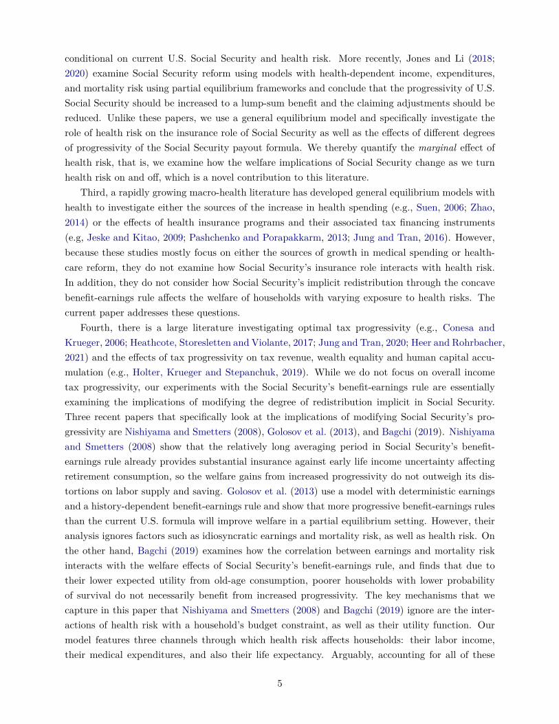
cj +aj+1

Health-dependent medical spending︷ ︸︸ ︷+oj (mj)+ 1[inj=1∧MAid-No]pEHI + 1[j≥Jr]pMCare +Ty (yj) +Tss (yn,j ; y) +TMCare (yn,j)

(7)

= (1 + r)aj +yn,j + 1[j≥Jr]bss,j (AIMEj) + bsi,j + b,

where β is a time preference factor, πj (hj) is the age and health state dependent survival probability,w is the market wage rate, r is the interest rate, oj is out-of-pocket medical spending, pEHI is theEHI premium, pMCare is the Medicare Plan B premium, after tax income is

yatj = yAGI,j−Ty (yj)−Tss (yn,j ; y)−TMCare (yn,j) , (8)

where Ty is the progressive income tax, which is a function of taxable household income yj , Tss isSocial Security’s payroll tax, also a function of labor income yn,j (up to a taxable maximum y), andTMCare is Medicare’s payroll tax. Labor income yn,j and total taxable income yj are defined as

yn,j = w

Health-dependent labor income︷ ︸︸ ︷×ej

(ϑ,εh,εn

)× nj , (9)

yAGI,j = yn,j + r×aj + 1[j≥Jr]bss,j (AIMEj) ,

yj = yAGI,j−1[inj=1∧MAid-No]pEHI−max[0,(oj (mj) + 1[j≥Jr]pMCare

)−0.075×yAGI,j

],

where yAGI,j is adjusted gross income. In addition, private health insurance premiums are taxdeductible as are out-of-pocket health expenses and Medicare premiums that exceed 7.5 percent ofyAGI.4 Social security payments are denoted bss,j and social transfers are defined as

bsi,j = max[0, c+oj (mj) + 1[inj=1∧MAid-No]pEHI + 1[j≥Jr]pMCare−yat

j −aj− b],

and ensure a minimum consumption floor c after medical expenses, insurance premiums and taxesare paid for. A household consuming at the lower bound cannot save into the next period. Accidentalbequests are denoted b.

Average past labor earnings follows

AIMEj+1 =

min(

(j−1)×AIMEj+yn,j

j , y)

if 1≤ j < Jr,

AIMEj if j ≥ Jr,

and

0≤ nj ≤ 1,

and Jr is the eligibility age for Social Security and Medicare. The indicator functions are defined4We assume 100 percent wage pass through from employers to employees so that the employer portion of health

insurance premiums is directly paid for by households. The tax deductibility is then also modeled on the householdside. Details about the tax deductibility of out-of-pocket expenses and Medicare premiums can be found in IRS(2010).

10

as 1[true] = 1 and 1[false] = 0.

Retired households. Households can stop working at any time, however they receive SocialSecurity benefits and qualify for Medicare starting at or after age j ≥ Jr and are forced to retire atage j ≥ JR, where Jr < JR. A retired households optimization problem reduces to

V (xj) = max{cj ,aj+1}

{u(cj) +β

(πj(εh)E [V (xj+1) |xj ] +

(1−πj

(εh))b(aj+1)

)}(10)

s.t.

cj +aj+1 +oj (mj) +pMCare +Ty (yj) = (1 + r)aj + bss,j (AIMEj) + bsi,j + b, (11)

where after tax income isyatj = yAGI,j−Ty (yj) , (12)

and adjusted gross income yAGI and taxable income yj are defined as

yAGI,j = r×aj + bss,j (AIMEj) .

yj = yAGI,j−max[0,(oj (mj) + 1[j≥Jr]pMCare

)−0.075×yAGI,j

].

Social transfers are expressed as

bsi,j = max[0, c+oj (mj) +pMCare−yat

j −aj− b].

Aggregation. We denote x≡ {j, xj} as the augmented state vector including age j and Λ(x)is the measure of households with state x which incorporates the relative cohort sizes µj .

3.9 Equilibrium

Given the transition probability matrices{

Πhj ,Πn

j

}Jj=1

, the survival probabilities{πj(εh)}J

j=1and

the exogenous government policies {Ty,Tss,TMCare, bsi, bss,κMCare,κMAid,G}Jj=1 , a stationary com-petitive equilibrium is a collection of sequences of distributions Λ(x) of individual household deci-sions{c(x) ,n(x) ,a(x)} , aggregate stocks of physical capital and effective labor services {K,L} , factorprices {w,q,R} , and insurance premiums premGHI such that:

(a) {c(x) ,n(x) ,a(x)} solves the consumer problem (6,7) ,

11

(b) the firm first order conditions hold in both sectors

w = ∂F (K,L)∂L

,

q = ∂F (K,L)∂K

,

R = 1 + q− δ = 1 + r,

(c) markets clear

K =∫a(x)dΛ(x) (13)

L=∫e(x)n(x)dΛ(x). (14)

TBeq =J∑j=1

µj

∫aj (xj)dΛ(xj) ,

(d) the aggregate resource constraint holds

G+K+∫

(c(x) +m(x))dΛ(x) = Y + (1− δ)K,

(e) the government programs clear so that (2) , (3) , and (4) hold,(f) the budget conditions of the insurance companies (5) hold and(g) the distribution is stationary

(µj+1,Λ(xj+1)) = Tµ,Λ (µj ,Λ(xj)) ,

where Tµ,Λ is a one period transition operator on the measure distribution

Λ(x′)= TΛ (Λ(x)) .

4 Calibration

We calibrate the model developed in the previous section to match the U.S. economy. We entertainmacroeconomic data targets such as overall capital accumulation, pattern of labor supply andhealth/medical expenditures over the life cycle, the life-cycle pattern of income heterogeneity, andalso the share of medical and government expenditures in GDP. While calibrating the model, we payspecial attention to the institutional details of Social Security, Medicare, and Medicaid, especiallythose relevant for its insurance effects against health risk.

For the calibration we distinguish between two sets of parameters: (i) externally selected pa-rameters and (ii) internally calibrated parameters. Externally selected parameters are estimatedindependently from our model and are either based on our own estimates using data from the

12

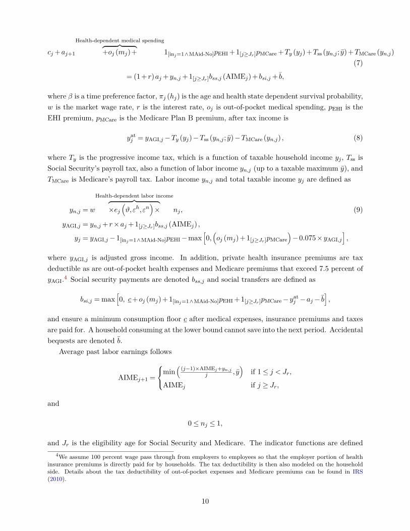
Medical Expenditure Panel Survey (MEPS) or the Panel Survey of Income Dynamics (PSID) orestimates provided by other studies. We summarize these external parameters in Table 1. Internallycalibrated parameters are assigned values so that model-generated data match a given set of targetsfrom U.S. data. These parameters are presented in Table 3. Model generated data moments andtarget moments from U.S. data are juxtaposed in Table 4.5

4.1 Demographics

One model period is defined as one year. We model households from age 25 to age 99 which resultsin J = 75 periods. The labor-supply choice periods are j ∈ [0, JR] = [0,60] which corresponds toages 25 and 84 respectively. Once the individual enters period 61, i.e. age 85, (s)he is forced toexit the labor force. We set the population growth rate to n = 0.01, and we distinguish betweenhealthy and sick individuals in terms of survival probabilities, which we define in Section 4.3 below.Panel [5] in Figure 1 shows our health-state-dependent survival probabilities, which we obtain fromestimates in İmrohoroğlu and Kitao (2012).

4.2 Preferences

We specify period utility as

u(cj , lj ; nj) =

(cηj ×

[1−nj− nj ·1[0≤nj ]

]1−η

)1−σ

1−σ .

We set the relative risk aversion parameter σ to 3, and the intertemporal discount factor β to0.998 to match the capital-output ratio target in equilibrium. Labor is chosen from a grid n ∈{0,nmin, ...,nmax} where the minimum amount of non-zero labor possible is nmin = 300 hours peryear, set to match the fraction of retirees at age 65 and the maximum amount of labor possibleis set to nmax = 80 work hours per week. The consumption intensity parameter η is 0.4 to matchaverage labor hours of the working population. The fixed cost of working nj is set to match thelabor participation rate by age group from PSID. 6

The warm-glow bequest function is

b(aj) = θ0(aj +θ1)(1−σ)η

1−σ ,

where θ1 determines the curvature of the function.7 We set θ1 = $500,000 as in De Nardi (2004)and French (2005) and scale parameter θ0 to match the asset holdings of retired individuals.

5Appendices A–B provide more detailed information about the data sources used.

6The Frisch labor elasticity in this model is

(1−nj+nj ·1[0≤nj ]

)n

(1−η(1−σ)

σ

)and given our parameter choice well

within the empirically estimated boundaries.7This warm-glow type bequest motive was first introduced by Andreoni (1989) and used in a general equilibrium

model in De Nardi (2004). A more sophisticated form of altruism would require an additional state variable andincrease the computational complexity.

13

4.3 Health status, health expenditure, and health insurance status

We use data from MEPS 1999–2017 to estimate the magnitude of the age dependent health ex-penditure shocks m

(j,εh

)as well as the Markov transition probability matrix Pr

(εhj+1|εhj

). We

group individuals into five health groups εh∈ {1,2,3,4,5} by self-reported health status: 1. excellenthealth, 2. very good health, 3. good health, 4. fair health, and 5. poor health. We then calculateaverage medical spending of each health group by age to determine the magnitude of the healthspending shocks m

(j,εh

). Since MEPS only accounts for about 65–70 percent of health care spend-

ing in the national accounts (see Sing et al., 2006; Bernard et al., 2012) we scale up the medicalspending profiles for individuals older than 65 similar to Pashchenko and Porapakkarm (2013).8

We next estimate an ordered logit model to determine the conditional probability of moving toa specific health group hg,j+1,t+1 in year t+1 conditional on being a member of health group hg,j,tat time t of a j year old individual using a fourth order age polynomial.9

Following Zhao (2014), we assume that the fraction of newborn households with employer pro-vided health insurance is 70 percent. At the age of 65 households become eligible for Medicare andare assumed to enroll in it. A household is eligible for Medicaid if it passes an earnings and anassets test, which can become their secondary insurance if they already have private insurance orMedicare. In rare cases, Medicaid may be tertiary insurance if households that are older than 65 arestill working and qualify for Medicare. In this case Medicare becomes primary insurance, privateemployer sponsored insurance is secondary, and Medicaid functions as tertiary insurance.

4.4 Income process

To calibrate the labor income process, we assume that labor productivity at age j can be decomposedas

ej(ϑ,εh,εn

)= ej

(ϑ,h

(εh))×εn, (15)

where ej(ϑ,h) is deterministic in age j, education level ϑ, and health state h, and εn is a stochasticcomponent that follows an auto-regressive process

ln(εnj

)= ρ× ln

(εnj−1

)+ εj , (16)

with persistence parameter ρ and a white-noise disturbance εj ∼N(0,σ2

ε

).

The h(εh)health state is binary and defined as

h(εh)

=

healthy if εh ∈ {1,2,3}

sick if εh ∈ {4,5}.

These are standard definitions for healthy/sick in the macro-health literature. The education level8Figure A.4 in Appendix A plots the distribution of health groups by age and Figure A.5 shows the associated

distribution of medical spending shocks by health group and age.9Figure A.3 in Appendix A depicts the conditional transition probabilities between the health groups.

14

is permanent and fixed at age 20. We define three permanent educational groups:

ϑ=

1 if less than high school,

2 if high school,

3 if college graduate or higher.

Figure 1 depicts the fraction of healthy individuals per age group and Table 44 shows the relativecohort sizes of healthy/sick types by permanent income group.

Stochastic component. To calibrate the stochastic component εn, we use ρ = 0.977 andσ2ε = 0.0141 based on estimates from French (2005) who uses PSID data and controls for cohort

effects and health states. We approximate the joint distribution of the persistent and transitoryshocks using a five-state first-order discrete Markov process following Tauchen and Hussey (1991).

Deterministic component. Using 1999–2017 MEPS data we construct cohort adjusted andbias corrected wage profiles for each subgroup (ϑ,h). Table 44 shows the relative cohort sizes ofthese types in the population. We use observations from the head of health insurance eligibility units(HIEU) and limit the sample by focusing on individuals with labor incomes larger than $400.10 Wethen use hourly wage observations of the head of a HIEU, deflate this variable with the urban CPIand remove cohort effects. We then follow the procedure in Rupert and Zanella (2015) and Casanova(2013) and estimate a selection model to remove the selection bias that is typically associated withwage observations to get an average wage offer rate for each (ϑ,h) subgroup. We finally smooth thewage profiles with a second degree polynomial in age.11

4.5 Technology and factor prices

We assume that output is produced using a Cobb-Douglas production function with inputs capitaland labor

Y =A×Kα×N (1−α), (17)

where α is the share of capital in total income. We set the capital share to α= 0.35 and the annualcapital depreciation rate to δ = 0.064, and normalize the total factor productivity A to unity.

4.6 Government

Taxes. The income tax function is progressive and has the following specification

Ty(y) = max[0, y− τ0×y(1−τ1)

],

10Labor income follows the definition in PSID and comprises wage income (variable WAGEP) and 75 percent ofbusiness income (variable BUSNP).

11Online Appendix A contains details about the procedures to remove cohort effects and wage biases.

15

where Ty(y) denotes net tax revenues as a function of pre-tax income y , τ1 is the progressivityparameter, and τ0 is a scaling factor to match U.S. income tax revenue.12 We impose a non-negative tax payment restriction in the benchmark model, Ty(y) ≥ 0. This restriction excludes allgovernment transfers embedded in the progressive tax function. Government transfers are explicitlymodeled in government spending programs.13

The Social Security system is self-financed via a payroll tax. The tax function is defined asTss (yn,j ; y) = τSS×max(yn,j , y) with τSS = 10.6 percent. The Social Security payroll tax is collectedon labor income up to a maximum contribution limit of $128,400 or 2.47 times median income.14

The Medicare system is also self-financed via a payroll tax and Medicare premium payments.The Medicare tax function is TMCare (yn,j) = τMCare× yn,j with τMCare = 2.9 percent. It is notrestricted by an upper limit (see SSA, 2007). Overall, the model results in total income tax revenueof 19.5 percent of GDP, Social Security tax revenue of 5.6 percent of GDP and Medicare tax revenueof 1.9 percent of GDP.

Expenditures. The government uses income tax revenue to make lump-sum transfers tomaintain a minimum level of consumption cmin of $2,700 (Pashchenko and Porapakkarm, 2013) andresidual unproductive government consumption of 15.2 percent of GDP.

Social Security. Households in the model start drawing Social Security benefits as well asMedicare benefits after 65. For each household, the government calculates an average of past earn-ings (up to the maximum taxable earnings), referred to as the Average Indexed Monthly Earnings(AIME). The Social Security benefit amount in 2010, also called the Primary Insurance Amount(PIA), is calculated as 90 percent of the first $761 of AIME, plus 32 percent of AIME over $761andthrough $4,586, plus 15 percent of AIME over $4,586 up to a maximum AIME of 2.47 of medianincome.15 We approximate this step function with the following parsimonious polynomial

bss(AIME) = a0×AIMEa1 (18)

and use a cap on the AIME of 2.47 times median income which corresponds to the maximum SocialSecurity payments. Parameter a1 = 0.567 determines the curvature of the Social Security benefit-

12This tax function is fairly general and captures the common cases:

(1) Full redistribution: Ty(y) = y− τ0 and T ′y(y) = 1 if τ1 = 1,

(2) Progressive: T ′y(y) = 1 −

<1︷ ︸︸ ︷(1 − τ1)τ0y(−τ1) and T ′y(y)> Ty(y)

y if 0< τ1 < 1,(3) No redistribution (proportional): Ty(y) = y− τ0y and T ′y(y) = 1 − τ0 if τ1 = 0,

(4) Regressive: Ty(y) = 1 −

>1︷ ︸︸ ︷(1 − τ1)τ0y(−τ1) and T ′y(y)< Ty(y)

y if τ1 < 0.

13This tax function was implemented into a dynamic setting by Benabou (2002) and more recently in Heathcote,Storesletten and Violante (2017). These authors do not model transfers explicitly and therefore allow income taxesto become negative for low income groups. We chose the tax curvature parameter τ1 = 0.15 which is very similar tothe one in Heathcote, Storesletten and Violante (2017) who, given the less explicit modeling of transfer payments intheir model, use a slightly more progressive tax function τ1 = 0.181.

14Compare contribution limits for Social Security contributions at https://www.ssa.gov/oact/cola/cbb.html15Compare SSA 2010 for bend points in the Social Security benefits formula at:

https://www.ssa.gov/oact/cola/bendpoints.html

16

earnings formula, and the scale parameter a0 adjusts so that Social Security’s budget is balancedwith the current payroll tax rate and the taxable maximum. Figure 2 depicts the PIA formula andthe polynomial approximation that we use in this paper. Total pension payments amount to 5.6percent of GDP in the baseline equilibrium, similar to the number reported in the budget tables ofthe Office of Management and Budget (OMB) for 2010. The distribution of pension payments isshown in Figure 5.16

Medicare and Medicaid. According to data from the National Health Expenditure Accounts(NHEA 2010) Medicare spending in 2010 was 3.5 percent of GDP and Medicaid spending (Federaland State) was 2.7 percent of GDP.17 Given reimbursement rates for Medicare κMCare from MEPSshown in Figure 3, the size of Medicare in the model is 4.8 percent. In order to qualify for Medicaid,households have to pass an earnings test, and we set the average eligibility threshold in the modelto 92 percent of the federal poverty level (FPL), which is close to the average state eligibility levelaccording to Kaiser (2013).18 In addition, a household has to pass an asset test so that its assetholdings are below the threshold of aMaid, which is calibrated to 150 percent of the FPL. Thereimbursement rate Medicaid κMAid depends on the medical spending level as can be seen in Figure3 which is based on data from MEPS. Using these reimbursement levels, Medicaid spending in themodel is about 2 percent of GDP, which is slightly lower than the 2.7 percent of GDP in NHEA2010.

4.7 Insurance companies

We set the reimbursement rate of private insurance companies κEHI according to MEPS data inFigure 3. EHI premiums pEHI clear the zero-profit condition (5) and result in annual premiumpayments of $6,190 in the baseline equilibrium. Claxton et al. (2010) report average annual pre-miums for employer-sponsored health insurance in 2010 are $5,049 for single coverage and $13,770for family coverage.

4.8 Model performance

The model is solved via backward iteration on discrete grids for assets, labor, and the earningshistory measure AIME. Table 4 and Figure 4 show the targeted moments of the calibration. Inaddition we perform checks of non-targeted data moments in Table 45 and Figure 6. The modelresults in medical spending as fraction of GDP of 16.5 percent which is close to the 17.3 percentreported in CMS data for 2010.19 The percent of workers on Medicaid is 10.7 and slightly higherthan the 9.6 percent reported in MEPS. The capital output ratio is 3.0, which is in the range ofstandard values of 2.9–3.24 in the calibration literature. The interest rate in the model is 5.3 percentwhich is also a standard value in the calibration literature (e.g., Prescott and Candler (2008)).

16Data for the Social Security benefits distribution in 2010 is from: https://www.ssa.gov/OACT/ProgData/benefits/ra_mbc201012.html17https://www.cms.gov/Research-Statistics-Data-and-Systems/Statistics-Trends-and-Reports/

NationalHealthExpendData/NationalHealthAccountsHistorical.html18Compare Remler and Glied (2001) and Aizer (2003) for additional discussions of Medicaid take-up rates.19Compare: https://www.cms.gov/Research-Statistics-Data-and-Systems/Statistics-Trends-and-Reports/

NationalHealthExpendData/NationalHealthAccountsHistorical.html

17

The model provides a reasonable fit for the lifecycle pattern of labor income (Figure 6) andlabor participation (Figure 5, Panel 1). The model reproduces the hump-shaped patterns of assetholdings as well as right skewed distributions of asset holdings, medical spending, and Social Securitytransfers. Gini coefficients of these variables are matched closely as shown in Table 5. Finally, themodel also shows weak negative correlations between medical spending and labor income as well asmedical spending and total income as shown in Figure 7.

5 Experiments

In order to examine the importance of idiosyncratic health risk in our calibrated general-equilibriummodel of Social Security, we compute two sets of experiments. In the first experiment, we cut SocialSecurity’s payroll tax rate from its baseline level of 10.6 percent to 5.3 percent (which is a 50 percenttax rate cut), while holding the taxable maximum income and the Social Security benefit-earningsformula constant. This experiment illustrates the overall consumption smoothing effect of SocialSecurity in a realistic incomplete-markets framework. In the second experiment, we hold SocialSecurity’s payroll tax rate and taxable maximum constant, and modify the progressivity of thebenefit-earnings formula via parameter a1. This experiment, on the other hand, highlights howthe degree of redistribution implicit in Social Security affects the welfare of households exposed tovarying degrees of income and health risk. Under both experiments, we correspondingly adjust thescale parameter a0 so that Social Security’s budget is balanced according to expression (2).

Because our goal is to understand how the specifics of the health risk environment shape SocialSecurity’s welfare effects in our framework, we compute the above two sets of experiments using thefollowing two versions of our model:

1. Baseline version: our original calibrated general-equilibrium model, with health risk affectinglabor income, expenditures, and also survival probabilities, and

2. No health risk version: a modified general-equilibrium model with idiosyncratic health riskremoved from labor income, expenditures, and also survivorship. In this modified framework,there is no within-cohort variation in the age-dependent component of labor productivity,medical expenditures, and the survival probability, conditional on health status.

These two versions of our model allow us to control the specific channels through which health riskaffects the household budget constraint and survivorship. It is also worth noting that switching fromthe Baseline version to the No health risk version of our model also requires some adjustmentsto the calibration so that the two models are comparable in terms of macro aggregates.

More specifically, in the No health risk version of the model, we first set the medical ex-penditures at every age equal to the average spending at that age across all households so thathealth spending follows a deterministic age profile, and aggregates to the same overall level ofhealth spending as in the Baseline model with idiosyncratic health spending. While this leaves theage-dependent component of health spending in the model, it turns off the idiosyncratic component.

Second, on the earnings side, we recalculate the labor productivity endowment function and re-move the correlation between health status εh and the age-dependent labor productivity endowment.

18

In order to accomplish this we recalculate the deterministic part ej(ϑ,h

(εh))

of the endowmentprocess in expression 15 and assign the average labor endowment over both sick and healthy typesfrom our baseline calibration to each education group so that the deterministic part now simplifiesto ej (ϑ) =

∫εh ej

(ϑ,h

(εh))dxj,εh where dxj,εh is the measure of the different health types of each

age group in the population.Finally, we calculate the average age-dependent conditional survival probability in the baseline

calibration across the healthy and sick, and then assign those probabilities to each age. Note thatthis adjustment automatically implies that the overall population size in this modified model isidentical to that in the Baseline model.

With these specification changes in place, our No health risk model corresponds to the canon-ical rational-expectations overlapping-generations framework that is routinely used to evaluate dy-namic public policy, but is augmented with a deterministic medical spending component to makeit comparable (in terms of macro aggregates) to our Baseline model that includes idiosyncratichealth risk. We do not otherwise recalibrate this model, hence the benchmark outcomes betweenthe model with and without health risk in Table 6 differ slightly.

In all of our experiments, we measure the welfare effects using a consumption equivalence varia-tion (CEV) measure, defined as a state-independent percentage change ∆C in period consumption,such that the discounted expected lifetime utility under the experiment equals the discounted ex-pected lifetime utility of the benchmark economy. Mathematically, ∆C solves

J∑j=1

µjβj−1

∫ πj(hBj

(xBj

))×u

((1 + ∆C)× cBj

(xBj

),nBj

(xBj

); nj ·1[nmin≤nB

j (xBj )])

+β(1−πj

(hBj

(xBj

)))× b

(aBj+1

)dΛ

(xBj

)

=J∑j=1

µjβj−1

∫ πj(hEj

(xEj

))×u

(cEj

(xEj

),nEj

(xEj

); nj ·1[nmin≤nE

j (xEj )])

+β(1−πj

(hEj

(xEj

)))× b

(aEj+1

)dΛ

(xEj

),

where superscripts B and E denote the baseline and the experiment, respectively. We also reportseparate CEV measures for each of the permanent income groups. Intuitively, this CEV measurecaptures the welfare gains (or losses) as percent of period consumption of a newly entering individual(i.e., a 25 year old in the model) under each one of our computational experiments. We also examinethe implications of these experiments for labor supply, consumption, and savings decisions, themarkets for goods and services, the values of key macroeconomic aggregates, and the government’sbudget.

5.1 Cutting Social Security’s Payroll Tax

First, what are the implications of cutting Social Security’s payroll tax rate in our model? Toevaluate this, we reduce the payroll tax from its baseline value of τSS = 10.6 percent to τSS = 5.3percent (a reduction of 50 percent) while keeping the remaining institutional features fixed. We

19

then adjust the scaling factor a0 of the Social Security benefit-earnings formula (16) to clear thebudget of the pension program in expression (2). We run this experiment twice: first using theBaseline version of our model with full idiosyncratic health risk, and then using the No healthrisk version of our baseline model.

5.1.1 Payroll tax rate reduction with health risk

We report the results of this experiment for the Baseline version of our model in the first twocolumns of Table 6. It is clear from the table that not surprisingly, downsizing Social Security in ourmodel environment leads to an overall welfare gain equivalent to 5.1 percent of period consumption,with larger welfare gains going to low- and middle-income households (CEVs of +4.6 and +5.7percent respectively). These welfare gains are driven primarily by increased labor supply andsaving, which leads to an increase in labor and capital of roughly 2.5 and 7.5 percent respectively.The effects on labor supply are driven by both labor participation (extensive margin) and laborhours of the working (intensive margin). The increase in effective labor is slightly stronger amongthe less educated who benefit the most from the increase of the overall wage rate of about 1.9percent. Labor participation rates, on the other hand, decrease slightly for the lowest income groupas more of them qualify for Medicaid. In general, as we scale back Social Security, individualsincrease their self insurance efforts. First, due to lower payroll taxes, they have more disposableincome, which is partly saved: capital owned by low- and middle-income households increase by16 and 10 percent respectively. Second, higher wage rates ultimately induce workers to lower theirlabor hours as income effects overpower substitution effects. This leads to a decrease of the averagelabor hours of the working population from 38.2 to 36.9 hours per week.

Social Security benefits of low- and middle-income households decrease by about 45 percent andconsumption insurance payments (referred to as Social Insurance at the bottom of Table 6) decreaseby about 5 percent. Due to these decreases in transfer payments, these households increase theirown savings and their effective labor supply, which, together with the increase in real wages, leadsto higher labor income. Despite the decreases in transfer payments, these growth effects are strongenough to result in overall welfare gains for the low- and medium-income households. High-incomehouseholds experience a larger drop in their Social Security benefits (about 54 percent), but due tothe fact that these households are significantly more self-insured to begin with, their labor supplyincreases by only 1.9 percent and their capital stock increases by 2.6 percent as a result of this taxcut.

Since health expenditures are exogenous, the increase in capital stock causes an expansion inoutput and as a result we observe a decline of the medical expenditures to GDP ratio from 16.5 to15.8 percent. As one would expect, the Gini coefficient of asset holdings slightly increases with thereduction in Social Security benefits, but the lower payroll tax causes the Gini coefficient of laborincome to slightly decrease.

It is worth noting that the above welfare result is consistent with the fact that in a generalequilibrium model with endogenous labor supply, Social Security’s distortionary welfare losses arelarger than the welfare gains from partial insurance against labor income and mortality risk (Bagchi,

20

2015).20 As expected, downsizing Social Security in our calibrated general-equilibrium environmentallows households to better harness their precautionary motive and self insure against health risk,and this effect is stronger for low- and middle-income households who are more likely to be borrowingconstrained because of the Social Security payroll tax.

To summarize, we find that downsizing Social Security under the current benefit-earnings for-mula and taxable maximum for the Social Security payroll tax leads to a welfare improvement.These welfare improvements are more pronounced for low income earners who can benefit morefrom higher income due to lower taxes. Given that our goal here is to examine the importance ofhealth risk in our framework, our next task is to evaluate these welfare effects in the No healthrisk version of our baseline model.

5.1.2 Payroll tax rate reduction in the absence of health risk

We next examine how a reduction in the size of Social Security affects welfare and the macroaggregates in the No health risk version of our baseline model. We previously introduced thismodel as one with no within-cohort variation in the age-dependent component of labor productivity,medical expenditures, and the survival probability, conditional on health status.

As before, for our experiment, we cut the Social Security payroll tax rate by 50 percent toτSS = 5.3 percent and let the scaling parameter a0 adjust to clear the Social Security budget inexpression (2), while keeping the curvature parameter a1 at its benchmark value. Table 6 showsthat similar to our baseline model, reducing the size of Social Security leads to a similar albeitsmaller increase in capital of about 7.1 percent, which translates into a 4.2 percent increase inoutput. In this experiment, a newly entering individual experiences a welfare gain of 5.4 percentof compensating consumption, which is not surprising given the structure of the model and itscalibration. However, this welfare gain is larger than what we find in our Baseline model under anidentical tax cut. In other words, downsizing Social Security appears to have a larger positive effecton welfare when we eliminate idiosyncratic health risk, which in turn suggests that Social Securityallows better consumption smoothing in a model environment with health risk.

Comparing the welfare effects of the payroll tax cut across permanent income groups, we findwelfare gains equivalent to 5.3 and 6.3 percent of compensating consumption for low- and middle-income households respectively in our No health risk model, which are larger than those obtainedin our Baseline model. Clearly, these households do not benefit as much from Social Security’sinsurance effects in the No health risk environment. High-income households, on the other hand,experience welfare gains equivalent to 3.3 percent of CEV in the No health risk environment,compared to 3.8 percent in the Baseline model. This should not be surprising, as the need foradditional self insurance through the precautionary motive is even less for these households in amodel framework that ignores health risk.

20Earlier studies analyzing the welfare effects of Social Security with models with inelastic labor supply report posi-tive welfare effects from Social Security that can disappear when discount factors are small (İmrohoroğlu, İmrohoroğluand Joines, 1995) or borrowing constraints are introduced (Hubbard and Judd, 1987). If we fix the intensive marginof labor supply in our model, we find slightly larger welfare effects from decreasing the Social Security payroll taxrate but overall the results are very similar.

21

Further evidence of the households’ varying precautionary responses to a 50 percent cut inSocial Security’s payroll tax is presented in Table 6. First, it should not come as a surprise thatin both models (Baseline and No health risk), the capital accumulation rates increase moreforcefully for low- and middle-income households. Since these households were more likely to beborrowing constrained and had a lower level of savings to begin with, their savings rate increases aredisproportionately larger than high-income households. Second, comparing the capital accumulationrates of the different household income types across the two models, we now observe a response incapital accumulation that mirrors the welfare results discussed earlier. College-educated householdsincrease their capital stock by 2.6 percent after the tax cut with health risk. This is roughly half apercentage point more than that without health risk, where the increase in capital stock is only 2.2.Contrary to this, households with only a high school degree (the middle income group) exhibit amuch smaller difference in capital accumulation between the model with health risk (a 9.6 percentincrease) and the model without health risk (a 9.4 percent increase). The capital accumulationnumbers for households with less than a high school degree are even closer, with 16.3 vs. 16.6percent increases with and without health risk, respectively.

In summary, we find that the presence of health risk in the model increases the importance ofSocial Security’s insurance effects, mostly because it allows low- and medium-income householdsto better smooth consumption in such an environment. A lower Social Security payroll tax leadsto increases in disposable income during early employment years, and allows households to betterself-insure against early-life health risk, but this effect dominates Social Security’s insurance effectsonly for high-income households who are already sufficiently self insured.21 Given the increases incapital and labor supply from the payroll tax cut, both with and without health risk, one mightconjecture that the welfare results discussed above are due to the general equilibrium effects ofthe policy experiments. However, it is important to remember that household-level consumptionsmoothing concerns are, in fact, the drivers of these general equilibrium effects. For example, if wecut Social Security’s payroll tax by 50 percent in partial equilibrium, i.e. holding capital, labor,wages and interest rates, insurance premia, and accidental bequests constant, households still gainin terms of overall welfare, but the gains are still smaller in the presence of health risk (3.8 percent)compared to without health risk (4.3 percent). This is because in partial equilibrium, the largerhousehold-level precautionary saving and labor supply responses to the presence of health risk arenot realized into a higher productive capacity for the economy, and subsequent higher consumptionlevels.

5.2 Changing the progressivity of Social Security’s benefit-earnings formula

One of the primary determinants of Social Security’s implicit insurance effects is the formula thatgoverns the relationship between a household’s past work-life income and the level of Social Security

21It is worth noting that because households with a history of adverse health shocks in our model are both poorerand more likely to die early, it is possible to argue that incorporating health risk causes Social Security to becomemore regressive than otherwise. As a result, it is conceivable that downsizing Social Security can improve welfareregardless of how it interacts with health risk. However, a careful comparison of the Health Risk and No HealthRisk columns in Table 6 shows that the labor income and asset Gini coefficients are roughly identical across the twobaselines, which suggests that this effect really does not play a role here.

22

benefits received during retirement. Currently, the U.S. benefit-earnings formula replaces 90 percentof the average work life earnings of households in the bottom 20 percent of the wage distributionbut only about 40–50 percent of average work life earnings of households with higher income. Thisconcavity in the benefit-earnings rule is intended to facilitate better work-retirement consumptionsmoothing for households that might experience unfavorable health and labor income shocks duringtheir work life. We now examine how health risk interacts with the welfare effects from modifyingthis benefit-earnings formula.

5.2.1 Social Security progressivity with health risk

We first evaluate how changing the curvature of Social Security’s benefit-earnings rule affects welfarein our Baseline model with health risk. To do this, we recompute our model under Social Security’scurvature parameter values a1 = 0.0 and 1.0 in expression (16). Figure 8 shows the payout formulafor various values of curvature parameter a1.

Functionally, parameter values a1 = 0 and a1 = 1 correspond to the two corner cases whereSocial Security benefits are either equal for all households and completely unrelated to past work-life income (a1 = 0), or where they are fully proportional (i.e., a linear function) to average work-lifeincome (a1 = 1). Also, note that in each experiment Social Security’s scale parameter a0 adjuststo balance the Social Security budget constraint under the current payroll tax rate, the taxablemaximum income, and the curvature parameter a1 under that experiment according to expression(2).22 We report the results from changing the curvature parameter a1 in our baseline model withhealth risk in Table 7.

Increasing PIA progressivity (a1 = 0). As is clear from Table 7, making Social Security’sbenefit-earnings rule more progressive compared to the benchmark economy (decreasing a1) leadsto a sharp drop in the Gini coefficient of Social Security payments from 0.27 to 0.13 and has anoverall positive effect on welfare equivalent to a 0.43 percent increase in period consumption.23 Thegains are largest at 1.3 percent of CEV for low-income households but the change to lump-sumpayments also generates losses of 1.7 percent of CEV for high-income households. Overall, thewelfare gain across all income groups is 0.5 percent of compensated consumption. There are twoprimary mechanisms behind these welfare gains.

First, the lump-sum pension payments trigger a positive effect on capital accumulation: anincrease of 2.4 percent in our Baseline model with health risk. This is mainly driven by low-and middle-income households, who save by 2.3− 2.6 percent more than in the baseline, despitereceiving pensions that are 16.2 and 7.5 percent higher than the baseline, respectively. High-incomehouseholds, on the other hand, experience the smallest increase in savings: switching to a lump-sum

22It should be noted here while it is theoretically possible to obtain a benefit-earnings formula that is more progres-sive than the lump-sum distribution with a1 = 0, we do not entertain such a formula in our analysis. Unconditionallump-sum transfers are often used as benchmarks as they are less distortionary than certain targeted transfers.

23This Gini coefficient is calculated using Social Security payments of older households. Since the model allowsfor early and late retirement, some of the older households are still working and do not receive any Social Securitypayments. For this reason even a system with lump-sum Social Security payments exhibits a Gini coefficient largerthan zero.

23

benefit unrelated to past income reduces their pension payments by almost 22 percent, and theyrespond by increasing their savings by 1.8 percent, as can be seen from the first column in Table 7.

At this point, it is worth pausing to inquire why low- and medium-income households save moredespite the increased insurance from Social Security. This is because the lump-sum pensions, eventhough more redistributive than the baseline, are still only available to households after age 65, andthere is still a considerable amount of consumption risk to smooth in early life. The fact that thesocial insurance (consumption floor) payments to low- and medium-income households increase by3.7 and 1.9 percent under this experiment supports this results, but additional precautionary savingis still needed to better smooth consumption.

Second, switching to lump-sum Social Security benefits also leads to a decline of almost 23percent in overall Medicaid expenditures. From a public finance viewpoint this is an interestingresult: a more equitable distribution of Social Security—a conditional transfer to the old—reducesconditional transfers to the poor. In addition, the social insurance program, which maintains aminimum consumption floor and represents the other transfer program to the poor, seems to workin tandem with Social Security. As the overall size of Social Security decreases slightly by 0.5percent, the size of Social Consumption Insurance increases by about 1.6 percent. Without thisincrease, it stands to reason that low income households may not have been able to gain fromincreased redistribution through the benefit-earnings rule.

In summary, we observe that improved risk sharing through the more equitable Social Securitysystem is welfare improving for households who experience relatively high income and health risk.24

These households tend to have lower income which compromises their ability to self insure, whichis reflected in the observed welfare gains from a lump-sum benefit-earnings rule that is unrelatedto past income. High-income households, on the other hand, are the losers under this experiment,which ultimately turns Social Security into a more progressive program.

Decreasing PIA progressivity (a1 = 1). Making Social Security’s benefit-earnings rule lessprogressive (increasing a1) reduces the implicit redistribution through Social Security and leads to awelfare loss of almost 0.6 percent of CEV overall. This is because with a linear (fully proportional)benefit-earnings rule, low- and medium-income households experience welfare losses equivalent to1.7 percent and 0.4 percent of CEV, and high-income households are almost indifferent between thecurrent U.S. rule and the fully proportional rule (CEV of −0.06 percent) as shown in Table 7.

With a linear payout formula the pension system does not redistribute wealth between thepermanent income groups as the returns from Social Security are proportional to the contributions tothe program.25 As a consequence, capital accumulation decreases by 1.7 percent as richer householdswith a relatively higher savings propensity can now recoup more of their pension contributionsupon retirement. We observe this from the much higher Social Security payments to high-incomehouseholds (an increase by 11 percent), which allows them to reduce their precautionary saving,

24The fraction of households classified as “sick” is shown in Panel [6] of Figure 1. Overall, the fraction of sickhouseholds is 9.8 percent as shown in Table 2.

25This is not quite accurate in our numerical setting where Social Security benefits are a function of AIME that arerecorded on a discrete grid. Depending on the grid size, there is always going to be a certain amount of grouping wherehouseholds with somewhat different income receive identical pension payments after retirement. In this sense, even aSocial Security benefits formula that is entirely proportional (i.e., a1 = 1) still retains a small element of redistribution.

24

thereby reducing their asset holdings by almost 3 percent. On the flip side, low- and middle-incomehouseholds experience a drop in their Social Security benefits of 9 and 5 percent respectively. Thismotivates them to save more to make up for the loss of insurance through Social Security. However,since the bulk of the capital stock is formed by savings of high income households, we observe adrop in the overall capital stock.

As a result, GDP decreases by about 0.4 percent. In addition, wages decrease as well as laborhours of the actively working decrease. These negative income effects cause some of the low-incomehouseholds to qualify for Medicaid which increases its size by 15.9 percent. Since high-incomehouseholds save less now, they have enough funds to maintain their consumption levels despitenegative income effects from lower wages. As a result, their welfare barely changes under thisexperiment. Poorer households are forced to save more and have to decrease their consumptionlevels. This leads to much larger welfare losses of almost 1.7 percent of CEV. In a sense thisreverses the welfare results we have observed earlier when Social Security payments were moreprogressive (i.e., lump-sum).

5.2.2 Social Security progressivity in the absence of health risk

In order to investigate how much of the above welfare effects can be specifically attributed to thepresence of health risk, we next compute the above experiments with the No health risk versionof our model.

Increasing PIA progressivity (a1 = 0). Even if idiosyncratic health risk is eliminated fromour baseline model (No health risk version in Table 7), we find that switching to lump-sumbenefits that are unrelated to past income leads to an overall welfare gain equivalent to 0.41 percentof CEV, which is smaller than the 0.43 percent of CEV welfare gain in the Baseline model withhealth risk. This happens despite a 4.0 percent increase in capital stock, which is larger than the2.4 percent increase in our the Baseline model, and a GDP increase of 1.25 percent in this case,which is also larger than the 0.7 percent increase in the Baseline model under the same policyexperiment. This result is driven by the fact that low-income households experience smaller welfaregains from the increased progressivity in the No health risk model: +1.2 of CEV, compared to+1.3 of CEV in our Baseline model. Clearly, making Social Security’s benefit-earnings rule moreprogressive increases welfare, but the effect is stronger in the environment with health risk.

Decreasing PIA progressivity (a1 = 1). When we switch to a linear (fully proportional)benefit-earnings rule without health risk, we find that overall welfare decreases by 0.35 percent ofCEV, with the largest welfare losses going to low-income households (CEV of −1.3 percent). Middle-income households are largely unaffected by this reduced progressivity (CEV gain of 0.17 percent).Comparing these to the welfare effects of the same experiment in our Baseline model, we find thatdecreasing the progressivity in Social Security’s benefit-earnings rule has a larger negative effect inthe presence of health risk (−0.6 percent of CEV). In other words, we once again find that SocialSecurity’s implicit insurance is relatively more important, especially to low- and medium-incomehouseholds, when health risk is present.

Decreasing the level of pension progressivity in the No health risk model decreases capital

25

stock by 2.55 percent, which is larger than the 1.75 percent decline in the Baseline model, andit also leads to an output loss of 0.77 percent, which is larger than the 0.37 percent decline in theBaseline model. Taken together, these results suggest that the measured changes in aggregatevariables are always larger in the No health risk version of our model. This should not besurprising, because precautionary motives are much stronger in the model with health risk. Anychange in Social Security’s implicit insurance would have a stronger effect on saving decisions inmodels with a weaker precautionary motive, as households will react to the changes in Social Securityunencumbered by any precautionary savings considerations. On the other hand, in an environmentwith a stronger precautionary motive in place, households will not adjust their saving as readily inreaction to changes in Social Security, as they will always factor in the precautionary reasons whenthey determine how much to save.

Finally, it is worth noting that the overall welfare effects of modifying Social Security’s benefit-earnings formula seem to suggest that additional insurance through a more progressive payoutformula is welfare improving, especially for low- and middle-income households that are at a higherrisk of ending up at the minimum consumption floor. In one of the earlier papers to investigate theinsurance component of Social Security, Nishiyama and Smetters (2008) conclude that the long aver-aging period of U.S. Social Security already provides substantial insurance against uninsured labor-market risks, which suggests that additional insurance through a more concave benefit-earnings rulewould be less important. We find evidence contrary to this result. Furthermore, if we make SocialSecurity less progressive and move to a proportional benefit-earnings formula, our model predictsoverall welfare losses despite the fact that high income individuals would prefer a linear payoutscheme over a lump-sum payout formula.

More recently, Bagchi (2019) examines how the positive correlation between income and lifeexpectancy interacts with the welfare implications of Social Security’s benefit-earnings formula.Using a model with differential mortality but without health risk he finds that the optimal benefit-earnings formula is slightly less concave than in the current US system, because the poor have lowerlife expectancy and therefore they heavily discount the utility from old-age consumption. In ourmodels with health spending, this is not the case: a more progressive Social Security payout formulaleads to welfare gains, and this is true for the version with and without idiosyncratic health risk.

The key mechanisms that we capture in this paper that Nishiyama and Smetters (2008) andBagchi (2019) ignore are the interactions of health risk with a household’s budget constraint, as wellas their utility function. Our model features three channels through which health risk affects house-holds: their labor income, their medical expenditures, and also their life expectancy. Nishiyamaand Smetters (2008) do not consider any of these channels in their welfare analysis of Social Se-curity’s benefit-earnings rule, thereby underestimating the riskiness of the environment in which ahousehold solves their life-cycle problem. Bagchi (2019), on the other hand, accounts for differentialmortality, i.e. the positive correlation between income and life expectancy, but does not accountfor how labor income and medical expenditures are affected by a household’s exposure to healthrisk. Arguably, accounting for all of these channels together within a calibrated general equilibriumenvironment leads us to quite different conclusions.

26

5.3 The role of risk aversion

As explained above, our computational results are driven by two primary mechanisms: the effect ofSocial Security on a household’s ability to better achieve work-retirement consumption smoothing,which is relatively long term, and the effect of idiosyncratic health risk on early-life consumptionsmoothing, which is relatively short term. Our results suggest that these mechanisms play outdifferently for households at different points in the income distribution. For low- and medium-incomehouseholds, Social Security’s long-term consumption smoothing benefits do seem to matter more,but for high-income households, the importance of short-term consumption smoothing appears tobe more important.

In a rational-expectations framework such as ours, a crucial determinant of a household’s pref-erence for better consumption smoothing is the coefficient of relative risk aversion, parameter σ,in the utility function. On the one hand, when risk aversion is high, households have more reasonto engage in precautionary saving so that consumption and leisure become less elastic to changesin policies such as Social Security. On the other hand, when risk aversion is low, households havea relatively low propensity for precautionary behavior and consumption and leisure become moreelastic. In this section, we evaluate the importance of risk aversion in the context of our compu-tational results. We are specifically interested in how different degrees of risk aversion affect therole of idiosyncratic health risk on welfare outcomes triggered by the discussed changes to SocialSecurity. To do this, we consider two additional alternative versions of our baseline model with riskparameters σ = 3: one with a higher risk aversion parameter σ = 3.5, and one with a lower riskaversion parameter σ = 2.5. We separately calibrate both models to our original macroeconomictargets and then perform the same set of computational experiments as before with each model.

Calibrating our baseline model with a higher coefficient of relative risk aversion of σ= 3.5 requiresus to adjust the discount factor to β = 1.001 so that the model matches our target capital-outputratio.26 Similarly, in the model with a lower coefficient of relative risk aversion of σ = 2.5 we haveto lower the discount factor to β = 0.986 to match the capital-output ratio.

5.3.1 Cutting Social Security

Similar to our earlier experiment we cut Social Security’s payroll tax rate from 10.6 to 5.3 percentin our newly calibrated models with different degrees of risk aversion.

Models with health risk. In the model with health risk and a higher risk aversion of σ = 3.5we again find that the payroll tax cut leads to an overall welfare gain equivalent to a CEV of 4.48percent, which is smaller than the welfare gain of 5.05 percent in the baseline calibration with a lowerrisk aversion of σ = 3.0 (see Table 8). The increase in aggregate capital in this case is 7.2 percent,which is slightly smaller than the increase of 7.5 percent in the baseline calibration, but the increasein consumption is somewhat larger: 6.4 percent, compared to 6.2 percent in the baseline calibration.The disaggregated welfare effects of this payroll tax cut with σ = 3.5 mirror those in the baselinecalibration with σ = 3.0: low- and middle-income households experience larger welfare gains, whichis consistent with the fact that these households are more likely to be borrowing constrained prior

26Note that this implies a slightly negative discount rate, which is common in the macro-calibration literature.

27

to the tax cut. The point to remember from this first experiment is that with a higher degree ofrisk aversion, cutting Social Security leads to smaller welfare gains across all income groups. Theprecautionary savings motive is stronger in this case so that household react less strongly to policychanges.

Second, when relative risk aversion is low with σ= 2.5, the tax cut leads to a much larger overallwelfare gain equivalent to 7.81 percent of CEV. This again corroborates our claim that risk aversionand welfare gains from cutting Social Security are inversely related. The fact that aggregate capitalmirrors this relationship supports our argument that precautionary savings plays a crucial role inour results. With higher levels of risk aversion, households’ capital positions are less sensitive tochanges in policies: the precautionary motive plays a moderating role with respect to householdsadjusting their savings.

Models without health risk. Table 9 shows the results of the same experiments in a modelwithout idiosyncratic health risk. Qualitatively the effects of welfare, output, and capital accumula-tion move in the same direction. However, without health risk the welfare effects tend to be smalleroverall if risk aversion is low. With rising degrees of risk aversion, the welfare effects between themodel with and without health risk begin to align more closely as demonstrated by the welfareresults in Tables 8 and 9.

In summary, we find that idiosyncratic health risk matters more for welfare in an environmentwith low risk aversion where households are more likely to react to changes in policy because ofweaker precautionary motives. With higher levels of risk aversion, the now stronger precautionarymotive mutes the effects caused by differences in health risk between the models in Table 8 and9 when it comes to welfare outcomes. Alternatively one could argue that with high risk aversion,Social Security causes weaker distortions and subsequent efficiency losses. Cutting Social Securityin such environments therefore leads to lower welfare gains as the program was less “distortive” tobegin with. The effects of idiosyncratic health risk therefore play a larger role in environments wherethe tax and savings distortions from Social Security are large enough so they can be subsequentlyamplified by the idiosyncratic health risk channels.

5.3.2 Changing the progressivity of Social Security

In this section we repeat the experiments from Section 5.2 and modify the progressivity of SocialSecurity’s benefit-earnings rule, holding the payroll tax rate and the taxable maximum incomethreshold constant, in models with different degrees of risk aversion.

Models with health risk. With a higher risk aversion of σ= 3.5, switching the Social Securitypayout formula to a lump-sum benefit leads to a very small overall welfare gain equivalent to a CEVof 0.06 percent (see Table 10). This is much smaller than the welfare gain of 0.43 percent CEV in ouroriginal baseline model calibrated with a lower degree of risk aversion of σ= 3.0. The smaller welfareeffect is both the result of smaller welfare gains of low- and medium-income households, and thelarger welfare losses of high-income households in this scenario with higher risk aversion. Overall, westill find that in the presence of health risk, increased progressivity does provide additional insuranceand welfare gains to low- and medium-income households, although the effect is considerably weaker

28

when we introduce a higher level of risk aversion. With lower risk aversion of σ = 2.5, we find thatswitching to a lump-sum benefits leads to an overall welfare gain equivalent to a CEV of 0.75percent. This is larger than the welfare gain of 0.43 percent CEV in our original baseline modelcalibrated with σ = 3. As an overall pattern, we can see that with rising levels of risk aversion, thewelfare results of all three income groups deteriorate.

On the other hand, switching to a linear (fully proportional) benefit-earnings rule causes awelfare loss of 0.57 percent of CEV with a higher risk aversion, as well as a very similar welfare lossof 0.54 percent in the model with a lower risk aversion. Both losses are slightly smaller than the0.6 percent loss with the baseline level of risk aversion of σ = 3. In addition, Table 10 shows that asrisk aversion increases, the welfare losses of low income groups increase when switching to the linearrule, but the losses of the middle and high income groups decrease. When risk aversion is highestat σ = 3.5 the highest income group actually starts experiencing a welfare gain from this policy. Inparticular, the linear payout rule hurts low income individuals in environments with higher levelsof risk aversion.

Models without health risk. When we remove idiosyncratic health risk and re-run theabove experiments, we find qualitatively similar welfare patterns for the two policy experimentsacross almost all income groups both with lower and higher risk aversion (compare Table 11).

However, comparing the above results with and without health risk, Tables 10 vs. 11, wefind that with a higher risk aversion of σ = 3.5, switching to a lump-sum benefit causes a smalleroverall welfare gain in the presence of health risk (0.06 percent), compared to when health risk iseliminated from the model (0.17 percent). It is interesting to point out that the magnitude of thewelfare effects (gains for low and middle income groups and losses for high income group) are largerin the presence of idiosyncratic health risk. This is not surprising: as individuals are more riskaverse, they gain more from lump-sum Social Security if idiosyncratic health risk exposes them toadditional uncertainty that is ameliorated by the more progressive pension payments. However, inthe aggregate the gains and losses from the different income groups cancel each other out so thatoverall we observe only very small welfare improvements in the model with health risk, compared tothe model without health risk. When risk aversion is lower, then idiosyncratic health risk mattersless for the low income group and their welfare gains are actually slightly smaller in the riskierenvironment with idiosyncratic health shocks. Their welfare gain from a more progressive SocialSecurity program is now only 1.59 compared to 1.93 percent when health shocks are absent.

Switching to a linear (fully proportional) benefit-earnings rule in the model with high riskaversion and no health shocks causes a welfare gain of 0.47 percent as opposed to a welfare loss of−0.57 percent in the model with health shocks. This result is mainly driven by the strong welfaregains of the high income types in the model without health risk who gain about 2.37 percent. Thisresults in much stronger capital accumulation and overall growth effects so that even the middleincome group experiences welfare gains when health shocks are absent. The precautionary motiveis weakened as the environment itself is now less risky. Households therefore react more stronglyto the linear payout rule of Social Security, which then increases output the subsequent increase inwelfare. Even with lower levels of risk aversion of σ = 2.5, we observe larger welfare effects from aless progressive Social Security program in the model without health shocks.

29

To summarize, our findings with respect to the role of risk aversion in our computational resultsfurther underscore the key mechanisms of our story. Social Security allows households to improvetheir work-retirement (long-term) consumption smoothing, but the payroll tax to fund Social Secu-rity negatively affects their early-life disposable income and worsens their short-term consumptionsmoothing ability. And when health risk affects labor income, household expenditures, and also lifeexpectancy, the relative strengths of these two mechanisms affect low income households differentlythan high income households. Modifying the coefficient of relative risk aversion allows us to examinehow changes in a household’s risk tolerance matters for the relative strengths of these two mech-anisms, and as expected, health risk matters less when households engage in more self-insurancedue to their stronger precautionary motives. On the other hand, when risk aversion is low, theprecautionary motive is weaker in the benchmark economy, so health risk matters more and theobserved overall welfare effects are larger in magnitude.

6 Conclusions

In conclusion, in this paper we quantify the importance of idiosyncratic health risk in a calibratedgeneral equilibrium model of Social Security. More specifically, we compare the welfare implicationsof Social Security in an environment with labor income, mortality, as well as health risks, to those inan environment where health risk is removed from the model. To do this, we begin by constructinga calibrated general-equilibrium macroeconomic model with households, firms, markets for goodsand services, and a government that provides partial insurance against income and health risks. Wethen compute two experiments using this calibrated model.

First, in order to evaluate the overall consumption smoothing effects of Social Security, we com-pute the effects of a 50 percent reduction in Social Security’s payroll tax rate. Second, in order toexamine how the degree of redistribution implicit in Social Security affects the welfare gains or lossesfor households with varying exposure to health risks, we compute the welfare effects of modifyingthe progressivity of Social Security’s benefit-earnings rule. Finally, we repeat these experiments ina hypothetical version of our model in which we remove health risk from the household’s economicenvironment. We also examine the implications of these experiments for labor supply, consump-tion, and saving decisions, the markets for goods and services, the values of key macroeconomicaggregates, and the government’s budget.

In general, our findings indicate that health risk has important implications for the welfare effectsof Social Security. The presence of partially insured health risk, especially in old age, increases theconsumption smoothing benefits of Social Security, but its payroll tax reduces disposable income inearly life, and negatively affects a household’s ability to self-insure against such risk. We find thatin our model framework, downsizing Social Security leads to higher welfare in general equilibrium,but the welfare gain is smaller when we account for health risk. We highlight that in a riskierenvironment precautionary savings motives are stronger and the distortions caused by taxes andpayouts related to the pension program are smaller. Downsizing a pension program that is less“distortive” to begin with therefore results in smaller welfare gains.

Similarly, modifying the progressivity of the benefit-earnings rule, we find that with health risk,

30

increased progressivity has a larger positive effect on overall welfare, and reduced progressivity hasa larger negative effect. In other words, our results suggest that ignoring the effect of health riskon labor income, household expenditures, and survivorship in a general-equilibrium environmentunderestimates the insurance value of Social Security.

Given that the key mechanism in our model is the trade-off between long- and short-term con-sumption smoothing, we examine how our computational results change with respect to a house-hold’s coefficient of relative risk aversion: the parameter that controls the strength of the precau-tionary motive. We find that as expected, when risk aversion is high, the precautionary motive isstronger in the benchmark economy, so Social Security’s welfare consequences are largely unaffectedby whether or not heath risk is present in the model environment. On the other hand, when riskaversion is low, the precautionary motive is weaker in the benchmark economy, so health risk mat-ters more for the welfare consequences. In fact, in this case the response to the presence of healthrisk is so large that households experience a larger welfare gain from downsizing Social Security inthe environment with health risk.

We leave human capital accumulation processes that can be affected by health investments forfuture analysis. In addition, we also assume stable demographic patterns and exogenous health risk.Modeling an endogenous health capital investment process that affects survival and productivity isleft for future research.

31

References

Abel, Andrew B. 1985. “Precautionary Saving and Accidental Bequests.” The American EconomicReview 75(4):777–791. 4

Aizer, Anna. 2003. “Low Take-Up in Medicaid: Does Outreach Matter and for Whom?” TheAmerican Economic Review 93(2):238–241. 17

Alonso-Ortiz, Jorge. 2014. “Social security and retirement across the OECD.” Journal of EconomicDynamics and Control 47(0):300–316. 2

Andreoni, James. 1989. “Giving with Impure Altruism: Applications to Charity and RicardianEquivalence.” Journal of Political Economy 97(6):1447–1458. 13

Auerbach, J. Alan and Laurence J. Kotlikoff. 1987. Dynamic Fiscal Policy. Cambridge: CambridgeUniversity Press. 2

Bagchi, Shantanu. 2015. “Labor supply and the optimality of Social Security.” Journal of EconomicDynamics and Control 58:167–185. 2, 20

Bagchi, Shantanu. 2019. “Differential Mortality and the Progressivity of Social Security.” Journalof Public Economics 177:104044. 5, 26

Bell, Felicity C. and Michael L. Miller. 2005. “Life Tables for the United States Social Security Area1900–2100.” Actuarial Study No. 116. Office of the Chief Actuary, Social Security Administration.August. 36

Benabou, Roland. 2002. “Tax and Education Policy in a Heterogeneous Agent Economy: WhatLevels of Redistribution Maximize Growth and Efficiency?” Econometrica 70(2):481–517. 16

Bernard, Didem, Cathy Cowan, Thomas Selden, Lining Cai, Aaron Catling and Stephen Heffler.2012. “Reconciling Medical Expenditure Estimates from the MEPS and NHEA, 2007.” Medicare& Medicaid Research Review 2(4):1–19. 14

Braun, R. Anton, Karen A. Kopecky and Tatyana Koreshkova. 2017. “Old, Sick, Alone and Poor: AWelfare Analysis of Old-Age Social Insurance Programs.” Review of Economic Studies 84:580–612.4

Casanova, Maria. 2013. “Revisiting the Hump-Shaped Wage Profile2013.” mimeo. 15, 51

Claxton, Gary, Bianca DiJulio, Benjamin Finder, Janet Lundy, Megan McHugh, Awo Osei-Anto,Heidi Whitmore, Jeremy Pickreign and Jon Gabel. 2010. Employer Health Benefits: 2010 AnnualSurvey. Kaiser Family Foundation and Health Research and Educational Trust. 17

Conesa, Juan C. and D. Krueger. 1999. “Social Security Reform with Heterogeneous Agents.” Reviewof Economic Dynamics 2:757–795. 8

32

Conesa, Juan C. and Dirk Krueger. 2006. “On the Optimal Progressivity of the Income Tax Code.”Journal of Monetary Economics 53(7):1425–1450. 5

Conesa, Juan Carlos and Carlos Garriga. 2009. “Optimal response to a transitory demographicshock in social security financing.” Federal Reserve Bank of St. Louis Review 91(1):33–48. 8

De Nardi, Mariacristina. 2004. “Wealth Inequality and Intergenerational Links.” Review of EconomicStudies 71:743–768. 13

French, Eric. 2005. “The Effects of Health, Wealth, and Wages on Labour Supply and RetirementBehaviour.” The Review of Economic Studies 72(2):395–427. 13, 15, 44

Glomm, Gerhard and Juergen Jung. 2013. “The Timing of Redistribution.” Southern EconomicJournal 80(1):50–80. 4

Golosov, Mikhail, Ali Shourideh, Maxim Troshkin and Aleh Tsyvinski. 2013. “Optimal PensionSystems with Simple Instruments.” American Economic Review 103(3):502–07. 5

Heathcote, Jonathan, Kjetil Storesletten and Giovanni L Violante. 2017. “Optimal Tax Progres-sivity: An Analytical Framework.” Quarterly Journal of Economics 132(4):1693–1754. 5, 16,44

Heer, Burkhard and Stefan Rohrbacher. 2021. “Endogenous longevity and optimal tax progressivity.”Journal of Health Economics 79:102515. 5

Holter, Hans A., Dirk Krueger and Serhiy Stepanchuk. 2019. “How Do Tax Progressivity andHousehold Heterogeneity Affect Laffer Curves?” Quantitative Economics 10:1317â–1356. 5

Hubbard, R. Glenn and Kenneth L. Judd. 1987. “Social Security and Individual Welfare: Precau-tionary Saving, Borrowing Constraints, and the Payroll Tax.” The American Economic Review77(4):630–646. 2, 4, 21

Huggett, Mark and Gustavo Ventura. 1999. “On the Distributional Effects of Social Security Re-form.” Review of Economic Dynamics 2(3):498–531. 8

İmrohoroğlu, Selahattin and Sagiri Kitao. 2012. “Social Security Reforms: Benefit Claiming, LaborForce Participation, and Long-run Sustainability.” American Economic Journal: Macroeconomics4(3):96–127. 13, 36, 44

İmrohoroğlu, Ayse, Selahattin İmrohoroğlu and Douglas H Joines. 1995. “A Life Cycle Analysis ofSocial Security.” Economic Theory 6(1):83–114. 2, 4, 21

İmrohoroğlu, Ayse, Selahattin İmrohoroğlu and Douglas H. Joines. 2003. “Time-Inconsistent Pref-erences and Social Security.” The Quarterly Journal of Economics 118(2):745–784. 8

İmrohoroğlu, Selahattin and Sagiri Kitao. 2012. “Social Security Reforms: Benefit Claiming, LaborForce Participation, and Long-Run Sustainability.” American Economic Journal: Macroeconomics4(3):96–127. 4

33

IRS. 2010. “Medical and Dental Expenses (including the Health Coverage Tax Credit).” Departmentof the Treasurey, Internal REvenue Service, Publication 502, Cat. No. 15002Q. 10

Jeske, Karsten. 2003. “Pension systems and aggregate shocks.” Federal Reserve Bank of AtlantaEconomic Review (Q1):15–31. 2, 8

Jeske, Karsten and Sagiri Kitao. 2009. “U.S. tax policy and health insurance demand: Can aregressive policy improve welfare?” Journal of Monetary Economics 56(2):210–221. 5

Jones, John Bailey and Yue Li. 2018. “The effects of collecting income taxes on Social Securitybenefits.” Journal of Public Economics 159:128–145. 5

Jones, John Bailey and Yue Li. 2020. Social Security Reform with Heterogeneous Mortality. WorkingPaper 20-09 Federal Reserve Bank of Richmond. 5

Jung, Juergen and Chung Tran. 2014. “Medical Consumption Over the Life Cycle: Facts from aU.S. Medical Expenditure Panel Survey.” Empirical Economics 47(3):927–957. 51

Jung, Juergen and Chung Tran. 2016. “Market Inefficiency, Insurance Mandate and Welfare: U.S.Health Care Reform 2010.” Review of Economic Dynamics 20:132–159. 5

Jung, Juergen and Chung Tran. 2020. “Health Risk, Insurance and Optimal Progressive IncomeTaxation.” Towson University, Department of Economics, Working Paper No. 2017-01. 5

Kaiser. 2013. “Where Are States Today? Medicaid and CHIP Eligibility Levels for Children andNon-Disabled Adults.” Kaiser Family Foundation Fact Sheet. 17

Kaplan, Greg. 2012. “Inequality and the Life Cycle.” Quantitative Economics 3(3):471–525. 51

Nishiyama, Shinichi and Kent Smetters. 2008. “The Optimal Design of Social Security Benefits.”Michigan Retirement Research Center Research Paper No. 2008-197. 5, 26

Pashchenko, Svetlana and Ponpoje Porapakkarm. 2013. “Quantitative Analysis of Health InsuranceReform: Separating Regulation from Redistribution.” Review of Economic Dynamics 16 (3):383–404. 5, 14, 16

Prescott, Edward C. and Graham V. Candler. 2008. Calibration. In The New Palgrave Dictionaryof Economics, ed. Steven N. Durlauf and Lawrence E. Blume. 2 ed. Palgrave Macmillan. 17

Remler, Dahlia K., Jason E. Rachling and Sherry A. Glied. 2001. “What Can the Take-Up of OtherPrograms Teach Us About How to Improve Take-Up of Health Insurance Programs?” NBERWorking Paper 8185. 17

Rupert, Peter and Giulio Zanella. 2015. “Revisiting wage, earnings, and hours profiles.” Journal ofMonetary Economics 72:114–130. 15, 51

Sing, Merrile, Jessica Banthing, Thomas Selden, Cathy Cowan and Sean Keehan. 2006. “ReconcilingMedical Expenditure Estimates from the MEPS and NHEA, 2002.” Health Care Financing Review28(1):25–40. 14

34

Smetters, Kent. 2003. Is the Social Security Trust Fund Worth Anything? Working Paper 9845National Bureau of Economic Research. 8

SSA. 2007. “Social Security Update 2007.” SSA Publication No. 05-10003. 16, 44

Suen, Richard M. H. 2006. “Technological Advance and the Growth in Health Care Spending.”Economie D’Avant Garde, Research Report No. 13. University of Rochester. 5

Tauchen, George and Robert Hussey. 1991. “Quadrature-Based Methods for Obtaining ApproximateSolutions to Nonlinear Asset Pricing Models.” Econometrica 59(2):371–396. 15

Wallenius, Johanna. 2013. “Social security and cross-country differences in hours: A general equi-librium analysis.” Journal of Economic Dynamics and Control 37(12):2466–2482. 2

Wooldridge, Jeffrey M. 1995. “Selection corrections for panel data models under conditional meanindependence assumptions.” Journal of Econometrics 68(1):115–132. 51

Zhao, Kai. 2014. “Social Security and the Rise in Health Spending.” Journal of Monetary Economics64:21–37. 5, 8, 14

35

Figures

30 40 50 60 70 80 90 1000

20

40

60

80

100%

[1] Health State

65 85

ExellentVery GoodGoodFairPoor

30 40 50 60 70 80 90 1000

50

100

150

200

$ 1,

000

[2] No HS: Medical Spending by Health State

65 85

12345 High

30 40 50 60 70 80 90 1000

50

100

150

200

$ 1,

000

[3] HS: Medical Spending by Health State

65 85

12345 High

30 40 50 60 70 80 90 1000

50

100

150

200

250

$ 1,

000

[4] College: Medical Spending by Health State

65 85

12345 High

30 40 50 60 70 80 90 1000

20

40

60

80

100

%

[5] Fraction Healthy

65 85MEPSModel

30 40 50 60 70 80 90 10050

60

70

80

90

100

%

[6] Survival Probabilities

65 85HealthySick

Figure 1: Exogenous health state process and health spending shocksNotes: Healthy is defined as the head of the HIEU reporting either Excellent, Very Good, or Good health. Sick isdefined as Fair or Poor health. Data source is MEPS 1999–2017, heads of HIEU, population weighted. The survivalprobabilities in panel [5] are from İmrohoroğlu and Kitao (2012) who base their estimates on data from the Healthand Retirement Study and life table estimates in Bell and Miller (2005). [back to 15, 24]

36

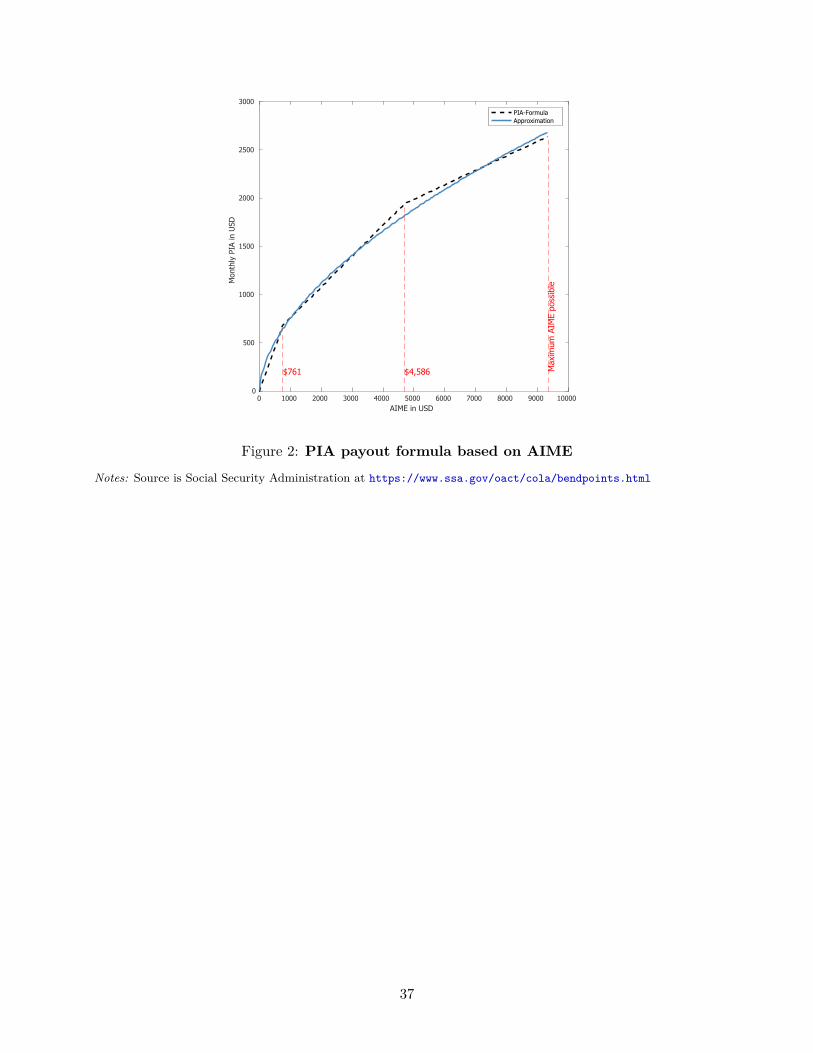
0 1000 2000 3000 4000 5000 6000 7000 8000 9000 10000AIME in USD

0

500

1000

1500

2000

2500

3000

Mon

thly

PIA

in U

SD

$761 $4,586 Max

imum

AIM

E po

ssib

le

PIA-FormulaApproximation

Figure 2: PIA payout formula based on AIME

Notes: Source is Social Security Administration at https://www.ssa.gov/oact/cola/bendpoints.html

37

0 5 10 15 20 25 30 35 40 45 50Medical Spending in $1,000

0

20

40

60

80

100

%

EHI Reimbursement Rates

0 5 10 15 20 25 30 35 40 45 50Medical Spending in $1,000

0

20

40

60

80

100

%

Medicaid Reimbursement Rates

0 5 10 15 20 25 30 35 40 45 50Medical Spending in $1,000

0

20

40

60

80

100

%

Medicare Reimbursement Rates

Figure 3: Exogenous health insurance reimbursement ratesNotes: Source is MEPS 1999–2017

38

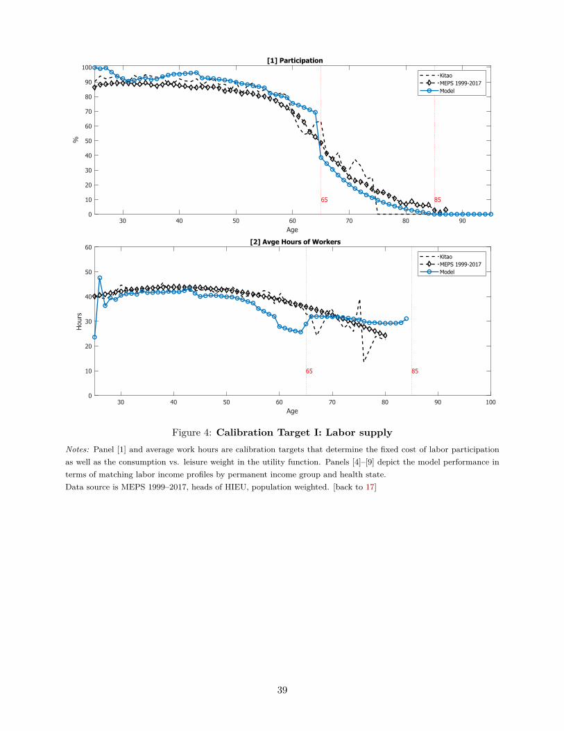
30 40 50 60 70 80 90Age

0

10

20

30

40

50

60

70

80

90

100%

[1] Participation

65 85

KitaoMEPS 1999-2017Model

30 40 50 60 70 80 90 100Age

0

10

20

30

40

50

60

Hou

rs

[2] Avge Hours of Workers

65 85

KitaoMEPS 1999-2017Model

Figure 4: Calibration Target I: Labor supplyNotes: Panel [1] and average work hours are calibration targets that determine the fixed cost of labor participationas well as the consumption vs. leisure weight in the utility function. Panels [4]–[9] depict the model performance interms of matching labor income profiles by permanent income group and health state.Data source is MEPS 1999–2017, heads of HIEU, population weighted. [back to 17]

39

30 40 50 60 70 80 90 100Age

0

50

100

150

%

[1] Avge. Med. Spend. % of Income

65 85

MEPSMEPS+CMSModel

25 30 35 40 45 50 55 60 65Age

0

20

40

60

80

100

%

[2] Fraction on Medicaid

MEPSModel

30 40 50 60 70 80 90 100Age

0

20

40

60

80

100

%

[3] Fraction Insured

65 85MEPSModel

Figure 5: Calibration Target II: Lifecycle profiles compared to dataNotes: These are not calibration targets. Data sources: is MEPS 1999–2017, heads of HIEU, population weighted.For asset data we use PSID 1999–2015. [back to 17]

40

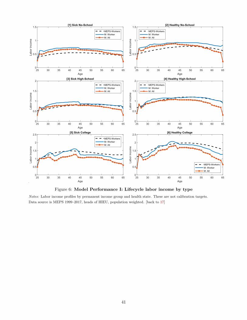
Figure 6: Model Performance I: Lifecycle labor income by typeNotes: Labor income profiles by permanent income group and health state. These are not calibration targets.Data source is MEPS 1999–2017, heads of HIEU, population weighted. [back to 17]

41

25 30 35 40 45 50 55 60 65-0.2

-0.1

0

0.1[1] Corr(M, Labor Income)

MEPSModel

30 40 50 60 70 80 90-0.2

-0.1

0

0.1[2] Corr(M, Income)

65 85

MEPSModel

Figure 7: Model Performance II: Distributions and lifecycle correlations compared todataNotes: These are not calibration targets. Data source is MEPS 1999–2017, heads of HIEU, population weighted.[back to 17]

42

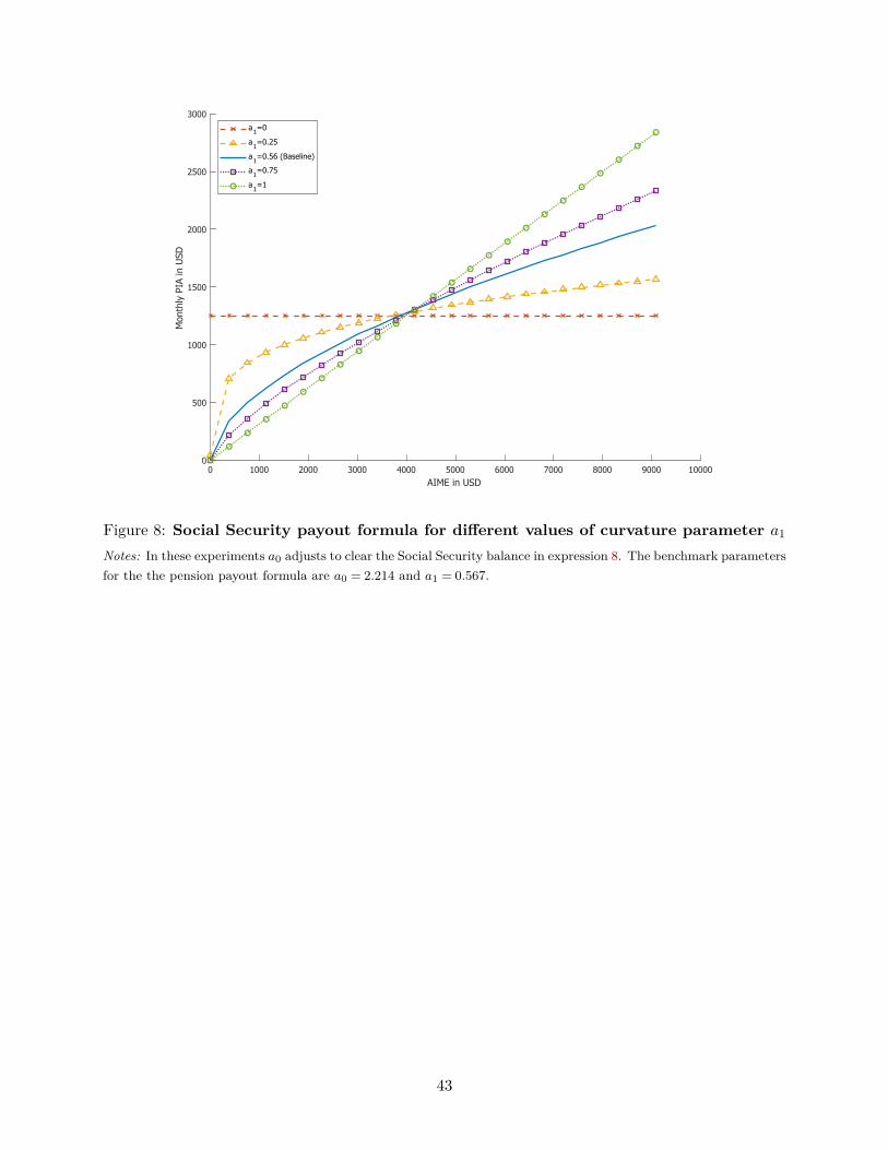
0 1000 2000 3000 4000 5000 6000 7000 8000 9000 10000AIME in USD

0

500

1000

1500

2000

2500

3000

Mon

thly

PIA

in U

SD

a1=0

a1=0.25

a1=0.56 (Baseline)

a1=0.75

a1=1

Figure 8: Social Security payout formula for different values of curvature parameter a1

Notes: In these experiments a0 adjusts to clear the Social Security balance in expression 8. The benchmark parametersfor the the pension payout formula are a0 = 2.214 and a1 = 0.567.

43

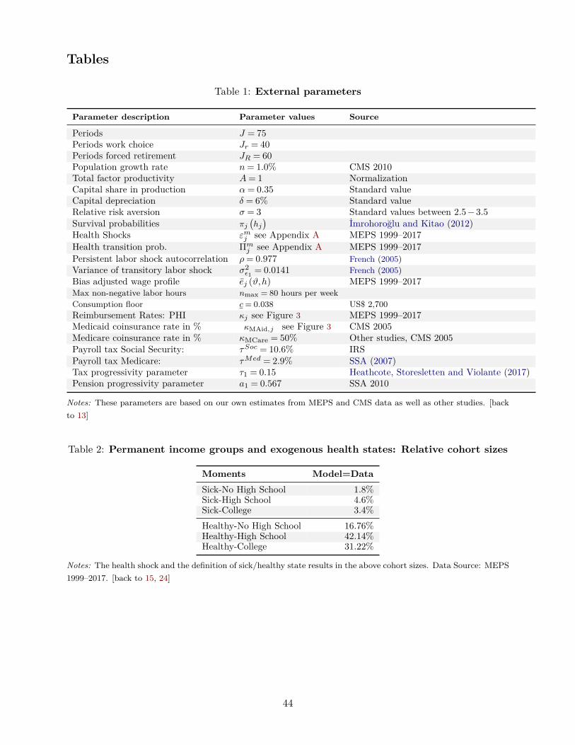
Tables

Table 1: External parameters

Parameter description Parameter values Source

Periods J = 75Periods work choice Jr = 40Periods forced retirement JR = 60Population growth rate n= 1.0% CMS 2010Total factor productivity A= 1 NormalizationCapital share in production α= 0.35 Standard valueCapital depreciation δ = 6% Standard valueRelative risk aversion σ = 3 Standard values between 2.5−3.5Survival probabilities πj

(hj)

İmrohoroğlu and Kitao (2012)Health Shocks εmj see Appendix A MEPS 1999–2017Health transition prob. Πmj see Appendix A MEPS 1999–2017Persistent labor shock autocorrelation ρ= 0.977 French (2005)Variance of transitory labor shock σ2

ε1 = 0.0141 French (2005)Bias adjusted wage profile ej (ϑ,h) MEPS 1999–2017Max non-negative labor hours nmax = 80 hours per weekConsumption floor c= 0.038 US$ 2,700Reimbursement Rates: PHI κj see Figure 3 MEPS 1999–2017Medicaid coinsurance rate in % κMAid,j see Figure 3 CMS 2005Medicare coinsurance rate in % κMCare = 50% Other studies, CMS 2005Payroll tax Social Security: τSoc = 10.6% IRSPayroll tax Medicare: τMed = 2.9% SSA (2007)Tax progressivity parameter τ1 = 0.15 Heathcote, Storesletten and Violante (2017)Pension progressivity parameter a1 = 0.567 SSA 2010

Notes: These parameters are based on our own estimates from MEPS and CMS data as well as other studies. [backto 13]

Table 2: Permanent income groups and exogenous health states: Relative cohort sizes

Moments Model=DataSick-No High School 1.8%Sick-High School 4.6%Sick-College 3.4%Healthy-No High School 16.76%Healthy-High School 42.14%Healthy-College 31.22%

Notes: The health shock and the definition of sick/healthy state results in the above cohort sizes. Data Source: MEPS1999–2017. [back to 15, 24]

44

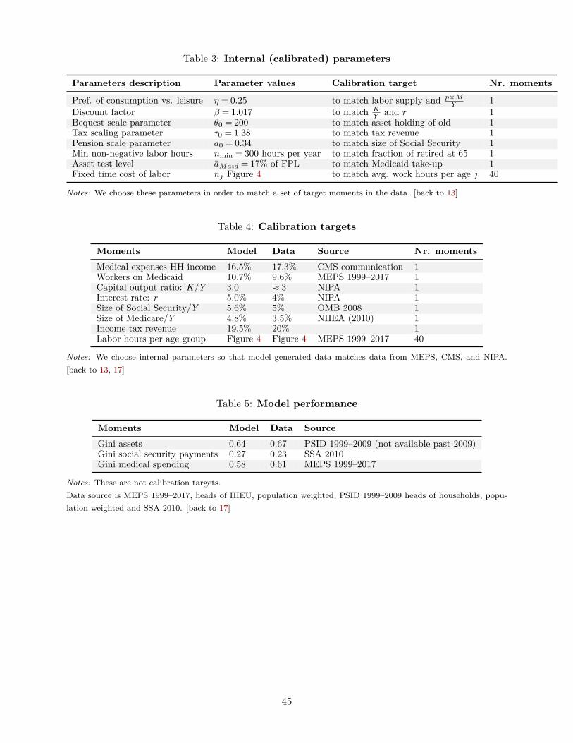
Table 3: Internal (calibrated) parameters

Parameters description Parameter values Calibration target Nr. moments

Pref. of consumption vs. leisure η = 0.25 to match labor supply and p×MY 1

Discount factor β = 1.017 to match KY and r 1

Bequest scale parameter θ0 = 200 to match asset holding of old 1Tax scaling parameter τ0 = 1.38 to match tax revenue 1Pension scale parameter a0 = 0.34 to match size of Social Security 1Min non-negative labor hours nmin = 300 hours per year to match fraction of retired at 65 1Asset test level aMaid = 17% of FPL to match Medicaid take-up 1Fixed time cost of labor nj Figure 4 to match avg. work hours per age j 40

Notes: We choose these parameters in order to match a set of target moments in the data. [back to 13]

Table 4: Calibration targets

Moments Model Data Source Nr. momentsMedical expenses HH income 16.5% 17.3% CMS communication 1Workers on Medicaid 10.7% 9.6% MEPS 1999–2017 1Capital output ratio: K/Y 3.0 ≈ 3 NIPA 1Interest rate: r 5.0% 4% NIPA 1Size of Social Security/Y 5.6% 5% OMB 2008 1Size of Medicare/Y 4.8% 3.5% NHEA (2010) 1Income tax revenue 19.5% 20% 1Labor hours per age group Figure 4 Figure 4 MEPS 1999–2017 40

Notes: We choose internal parameters so that model generated data matches data from MEPS, CMS, and NIPA.[back to 13, 17]

Table 5: Model performance

Moments Model Data SourceGini assets 0.64 0.67 PSID 1999–2009 (not available past 2009)Gini social security payments 0.27 0.23 SSA 2010Gini medical spending 0.58 0.61 MEPS 1999–2017

Notes: These are not calibration targets.Data source is MEPS 1999–2017, heads of HIEU, population weighted, PSID 1999–2009 heads of households, popu-lation weighted and SSA 2010. [back to 17]

45

Table 6: Social Security tax cut by 50 percent with and without health risk

Health risk No health risk

τss = 10.6% τss = 5.3% τss = 10.6% τss = 5.3%Benchmark Reduced Pension Benchmark Reduced Pension

Output Y 100 104.22 100 104.21Capital K 100 107.50 100 107.10Consumption C 100 106.21 100 106.46K/Y 3.01 3.10 3.04 3.12M/Y % 16.47 15.80 16.41 15.76Avge hours/week workers 38.21 36.91 38.31 36.93Social Security 100 51.95 100 52.32Medicare 100 100.00 100 100.00Medicaid 100 129.30 100 133.88Social Ins 100 94.26 100 95.04Interest rate r 0.05 0.05 0.05 0.05Wages w 100 101.88 100 101.60Gini labor income 0.65 0.64 0.65 0.64Gini assets 0.64 0.65 0.64 0.65Gini soc.sec. payments 0.27 0.36 0.26 0.36Gini medical spending 0.58 0.58 0.50 0.50Welfare All %C 0 5.05 0 5.44

Effects by income group Effects by income group

Welf. No HiSchool 0 4.57 0 5.27Welf. HiSchool 0 5.71 0 6.33Welf. College 0 3.76 0 3.26Capital No HiSchool 100 116.28 100 116.64Capital HiSchool 100 109.60 100 109.35Capital College 100 102.64 100 102.15Labor No HiSchool 100 102.20 100 102.20Labor HiSchool 100 102.81 100 102.44Labor College 100 101.93 100 103.29Avge. Part. No HiSchool 100 99.87 100 99.55Avge. Part. HiSchool 100 100.12 100 100.04Avge. Part. College 100 100.58 100 100.19Social Security No HiSchool 100 55.38 100 55.72Social Security HiSchool 100 54.99 100 55.72Social Security College 100 46.19 100 46.08Social Insurance No HiSchool 100 95.17 100 95.97Social Insurance HiSchool 100 94.95 100 96.03Social Insurance College 100 93.57 100 94.19

Notes:Health risk model has idiosyncratic health spending shocks and health affects labor productivity.No health risk model has no health spending shocks and income is independent of health. Medical spending inthis model is deterministic and depends on age and the permanent income group. We chose the magnitude of thesehealth spending shocks to be equal to the average health spending shock of the same age/permanent income typeas in the model with full health risk. Due to the resulting lower variation in health spending, the Gini coefficient ofhealth spending in the model without health risk is lower. We have not recalibrated the benchmark version of theno-risk model, therefore the benchmark versions of the two models shown above show slight differences in some of theaggregate moments. [back to 21]

46

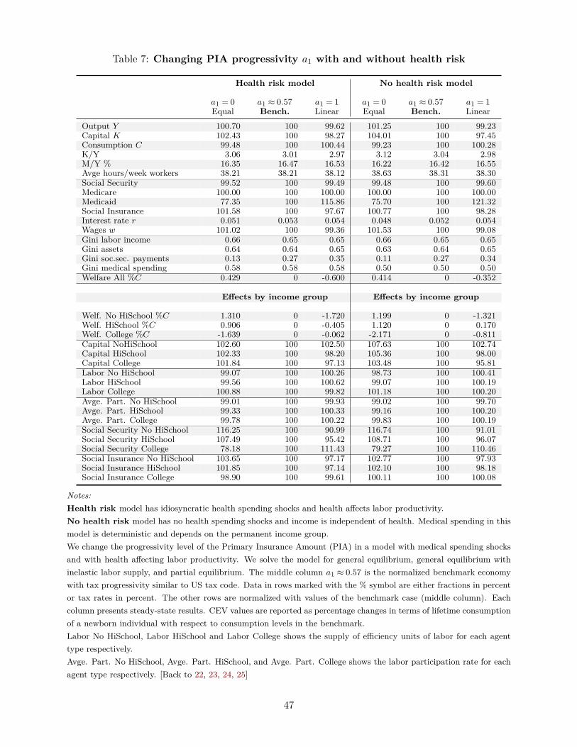
Table 7: Changing PIA progressivity a1 with and without health risk

Health risk model No health risk model

a1 = 0Equal

a1 ≈ 0.57Bench.

a1 = 1Linear

a1 = 0Equal

a1 ≈ 0.57Bench.

a1 = 1Linear

Output Y 100.70 100 99.62 101.25 100 99.23Capital K 102.43 100 98.27 104.01 100 97.45Consumption C 99.48 100 100.44 99.23 100 100.28K/Y 3.06 3.01 2.97 3.12 3.04 2.98M/Y % 16.35 16.47 16.53 16.22 16.42 16.55Avge hours/week workers 38.21 38.21 38.12 38.63 38.31 38.30Social Security 99.52 100 99.49 99.48 100 99.60Medicare 100.00 100 100.00 100.00 100 100.00Medicaid 77.35 100 115.86 75.70 100 121.32Social Insurance 101.58 100 97.67 100.77 100 98.28Interest rate r 0.051 0.053 0.054 0.048 0.052 0.054Wages w 101.02 100 99.36 101.53 100 99.08Gini labor income 0.66 0.65 0.65 0.66 0.65 0.65Gini assets 0.64 0.64 0.65 0.63 0.64 0.65Gini soc.sec. payments 0.13 0.27 0.35 0.11 0.27 0.34Gini medical spending 0.58 0.58 0.58 0.50 0.50 0.50Welfare All %C 0.429 0 -0.600 0.414 0 -0.352

Effects by income group Effects by income group

Welf. No HiSchool %C 1.310 0 -1.720 1.199 0 -1.321Welf. HiSchool %C 0.906 0 -0.405 1.120 0 0.170Welf. College %C -1.639 0 -0.062 -2.171 0 -0.811Capital NoHiSchool 102.60 100 102.50 107.63 100 102.74Capital HiSchool 102.33 100 98.20 105.36 100 98.00Capital College 101.84 100 97.13 103.48 100 95.81Labor No HiSchool 99.07 100 100.26 98.73 100 100.41Labor HiSchool 99.56 100 100.62 99.07 100 100.19Labor College 100.88 100 99.82 101.18 100 100.20Avge. Part. No HiSchool 99.01 100 99.93 99.02 100 99.70Avge. Part. HiSchool 99.33 100 100.33 99.16 100 100.20Avge. Part. College 99.78 100 100.22 99.83 100 100.19Social Security No HiSchool 116.25 100 90.99 116.74 100 91.01Social Security HiSchool 107.49 100 95.42 108.71 100 96.07Social Security College 78.18 100 111.43 79.27 100 110.46Social Insurance No HiSchool 103.65 100 97.17 102.77 100 97.93Social Insurance HiSchool 101.85 100 97.14 102.10 100 98.18Social Insurance College 98.90 100 99.61 100.11 100 100.08

Notes:Health risk model has idiosyncratic health spending shocks and health affects labor productivity.No health risk model has no health spending shocks and income is independent of health. Medical spending in thismodel is deterministic and depends on the permanent income group.We change the progressivity level of the Primary Insurance Amount (PIA) in a model with medical spending shocksand with health affecting labor productivity. We solve the model for general equilibrium, general equilibrium withinelastic labor supply, and partial equilibrium. The middle column a1 ≈ 0.57 is the normalized benchmark economywith tax progressivity similar to US tax code. Data in rows marked with the % symbol are either fractions in percentor tax rates in percent. The other rows are normalized with values of the benchmark case (middle column). Eachcolumn presents steady-state results. CEV values are reported as percentage changes in terms of lifetime consumptionof a newborn individual with respect to consumption levels in the benchmark.Labor No HiSchool, Labor HiSchool and Labor College shows the supply of efficiency units of labor for each agenttype respectively.Avge. Part. No HiSchool, Avge. Part. HiSchool, and Avge. Part. College shows the labor participation rate for eachagent type respectively. [Back to 22, 23, 24, 25]

47

Table 8: Risk aversion and Social Security tax cut with health risk

σ = 2.5 Benchmark σ = 3.0 σ = 3.5τss = 10.6% τss = 5.3% τss = 10.6% τss = 5.3% τss = 10.6% τss = 5.3%

Output Y 100.000 104.082 100.000 104.215 100.000 104.323Capital K 100.000 108.355 100.000 107.496 100.000 107.185Consumption C 100.000 105.934 100.000 106.206 100.000 106.423Avge hours/week workers 39.435 37.942 38.211 36.913 36.729 35.791Social Security 100.000 52.712 100.000 51.948 100.000 52.227Medicaid 100.000 128.963 100.000 129.302 100.000 128.867Social Ins 100.000 93.772 100.000 94.260 100.000 94.565Welfare All %C 0.000 7.810 0.000 5.048 0.000 4.482Welf. No HiSchool 0.000 8.286 0.000 4.565 0.000 3.747Welf. HiSchool 0.000 8.341 0.000 5.711 0.000 5.11Welf. College 0.000 6.108 0.000 3.763 0.000 3.477

Notes: The first columns with τss = 10.6% are the normalized benchmark economies with payroll taxes similar toUS tax code. The other columns are normalized with the respective benchmark. Each column presents steady-stateresults. CEV values are reported as percentage changes in terms of lifetime consumption of a newborn individualwith respect to consumption levels in the benchmark. [back to 27]

Table 9: Risk aversion and Social Security tax cut without health risk

σ = 2.5 Benchmark σ = 3.0 σ = 3.5τss = 10.6% τss = 5.3% τss = 10.6% τss = 5.3% τss = 10.6% τss = 5.3%

Output Y 100.000 104.059 100.000 104.209 100.000 106.222Capital K 100.000 108.069 100.000 107.096 100.000 111.975Consumption C 100.000 106.082 100.000 106.455 100.000 107.649Avge hours/week workers 39.705 38.099 38.314 36.929 37.239 35.469Social Security 100.000 52.533 100.000 52.320 100.000 53.573Medicaid 100.000 132.438 100.000 133.744 100.000 109.874Welfare All %C 0.000 7.461 0.000 5.435 0.000 4.486Welf. No HiSchool 0.000 7.954 0.000 5.267 0.000 3.872Welf. HiSchool 0.000 8.053 0.000 6.326 0.000 4.593Welf. College 0.000 5.592 0.000 3.258 0.000 4.840

Notes: The first columns with τss = 10.6% are the normalized benchmark economies with payroll taxes similar toUS tax code. The other columns are normalized with the respective benchmark. Each column presents steady-stateresults. CEV values are reported as percentage changes in terms of lifetime consumption of a newborn individualwith respect to consumption levels in the benchmark. [back to 28]

48

Table 10: Risk aversion and PIA progressivity with health risk

σ = 2.5 Benchmark σ = 3.0 σ = 3.5a1 = 0 a1 ≈ 0.57 a1 = 1 a1 = 0 a1 ≈ 0.57 a1 = 1 a1 = 0 a1 ≈ 0.57 a1 = 1

Output Y 100.493 100.000 99.694 100.696 100.000 99.622 100.843 100.000 99.497Capital K 101.842 100.000 98.639 102.425 100.000 98.278 102.861 100.000 97.693Consumption C 99.387 100.000 100.308 99.483 100.000 100.437 99.312 100.000 100.407Avge hours/week workers 39.573 39.435 39.278 38.212 38.211 38.122 36.947 36.729 36.948Social Security 100.756 100.000 100.028 99.524 100.000 99.489 99.466 100.000 99.927Medicaid 79.337 100.000 116.241 77.354 100.000 115.862 77.955 100.000 116.491Social Ins 101.645 100.000 97.309 101.578 100.000 97.671 101.465 100.000 98.023Welfare All %C 0.751 0.000 -0.538 0.429 0.000 -0.600 0.062 0.000 -0.566Welf. No HiSchool 1.591 0.000 -1.205 1.310 0.000 -1.720 0.753 0.000 -2.057Welf. HiSchool 1.178 0.000 -0.454 0.906 0.000 -0.405 0.566 0.000 -0.298Welf. College -1.006 0.000 -0.177 -1.639 0.000 -0.062 -2.113 0.000 0.244

Notes: The middle columns with a1 ∼ 0.57 are the normalized benchmark economies with tax progressivity similar toUS tax code. The other columns are normalized with the respective benchmark. Each column presents steady-stateresults. CEV values are reported as percentage changes in terms of lifetime consumption of a newborn individualwith respect to consumption levels in the benchmark. [back to 28]

Table 11: Risk aversion and PIA progressivity without health risk

σ = 2.5 Benchmark σ = 3.0 σ = 3.5a1 = 0 a1 ≈ 0.57 a1 = 1 a1 = 0 a1 ≈ 0.57 a1 = 1 a1 = 0 a1 ≈ 0.57 a1 = 1

Output Y 100.805 100.000 99.501 101.246 100.000 99.233 103.089 100.000 100.959Capital K 102.856 100.000 98.106 104.012 100.000 97.448 109.101 100.000 102.091Consumption C 99.371 100.000 100.155 99.229 100.000 100.280 100.198 100.000 101.276Avge hours/week workers 39.837 39.705 39.572 38.626 38.314 38.299 37.125 37.239 37.001Social Security 100.831 100.000 99.364 99.486 100.000 99.595 100.867 100.000 102.153Medicaid 77.476 100.000 118.320 75.702 100.000 121.322 64.766 100.000 103.189Welfare All %C 1.189 0.000 -0.876 0.414 0.000 -0.352 0.174 0.000 0.468Welf. No HiSchool 1.925 0.000 -1.538 1.199 0.000 -1.321 0.363 0.000 -1.100Welf. HiSchool 1.781 0.000 -0.706 1.120 0.000 0.170 0.350 0.000 0.407Welf. College -0.877 0.000 -0.725 -2.171 0.000 -0.811 -0.530 0.000 2.367

Notes: The middle columns with a1 ∼ 0.57 are the normalized benchmark economies with tax progressivity similar toUS tax code. The other columns are normalized with the respective benchmark. Each column presents steady-stateresults. CEV values are reported as percentage changes in terms of lifetime consumption of a newborn individualwith respect to consumption levels in the benchmark. [back to 29]

49

Online Appendix:Health Risk and the Welfare Effects of SocialSecurity

A Medical Expenditure Panel Survey (MEPS)

We primarily use data from the Medical Expenditure Panel Survey (MEPS) from the years 1999–2017for our estimation and calibration. MEPS provides a nationally representative survey about healthcare use, health expenditures, health insurance coverage as well as demographic data on income,health status, and other socioeconomic characteristics. The original household component of MEPSwas initiated in 1996. Each year about 15,000 households are selected and interviewed five timesover two full calendar years. MEPS groups individuals into Health Insurance Eligibility Units(HIEU) which are subsets of households. We do abstract from family size effects and concentrateon adults aged 20–85 who are the head of the HIEU.

A.1 Health care expenditure data

MEPS provides high quality health expenditure and health care utilization data. The MEPS House-hold Component (HC) collects data in each round on use and expenditures for office- and hospital-based care, home health care, dental services, vision aids, and prescribed medicines. In addition, theMEPS Medical Provider Component (MPC) is a follow-back survey that collects data from a sampleof medical providers and pharmacies that were used by sample persons in a given year. Expendi-ture data collected in the MPC are generally regarded as more accurate than information collectedin the HC and are used to improve the overall quality of MEPS expenditure data. Expendituresin MEPS refer to what is paid for health care services. Expenditures are defined as the sum ofdirect payments for care provided during the year, including out-of-pocket payments and paymentsby private insurance, Medicaid, Medicare, and other sources. Payments for over-the-counter drugsare not included in MEPS and neither are payments for long-term care. Similarly payments notrelated to specific medical events, such as Medicaid Disproportionate Share and Medicare DirectMedical Education subsidies, are also not included. MEPS records actual payments made and notoriginal charges which tend to be much higher. However, it has become customary to apply dis-counts. In addition charges associated with uncollected liabilities, bad debt and charitable care donot constitute actual health care expenses and are therefore not counted.

A.2 Cohort effects

Panel data variables over the lifecycle of an individual are determined by age, time and cohorteffects. Since our model only explicitly accounts for age effects, we should ideally remove time andcohort effects from the data in order to make lifecycle observations from the data consistent withlifecycle statistics generated by the model. Since age, time and cohort effects are perfectly collinear

50

it is difficult to estimate all three simultaneously (e.g., Jung and Tran (2014)). The literature (e.g.,Kaplan (2012)) often suggests to conduct separate analyses once controlling for the cohort effectand in a repeat exercise controlling for the time effect. In this work we explicitly control for cohorteffects of wages, income and health expenditures by regressing the log of the output variable on aset of age and cohort dummies. We focus on controlling for cohort effects because according to Jungand Tran (2014) they seem to be large in health expenditure data and time effects can be somewhatmitigated by deflating with the CPI index. We then use predictions of these regressions to generatea cohort-adjusted variable by predicting for a base cohort, that is we leave out the cohort dummiesin the prediction.

Summary statistics of the unweighted sample are presented in Table A.1 and a histogram of theage distribution is presented in Figure A.1. All dollar values are denominated in 2010 dollars usingthe OECD CPI for the US for all monetary measures.27

A.3 Unbiased wage profiles

We follow Rupert and Zanella (2015) and Casanova (2013) and estimate a selection model to removebiases in self reported wages. Rupert and Zanella (2015) use PSID and CPS data and then employa Tobit 2-step procedure based on Wooldridge (1995) to estimate selection corrected wage profiles.They find that once wage profiles are bias corrected they tend to be very flat which contradictsthe often used hump-shaped wage profiles. Similarly, Casanova (2013) uses HRS data and findsevidence of flat wage profiles but no selection bias.

In our selection model we include fourth order polynomials in age, health status, whether some-one lives with a partner, family size, schooling, gender, and an indicator for part-time work. Weuse indicator variables for whether an individual is older than 62 and a second indicator variable forwhether an individual is older 65 in the selection equation as is customary in this literature. Thesetwo indicator variables are exclusion restrictions and not included in the outcome equation of theselection model. Figure A.6 shows the wage profiles for healthy and unhealthy types and the threeeducational groups.

27OECD (2018), Inflation (CPI) (indicator). doi: 10.1787/eee82e6e-en (Accessed on 29 June 2018) athttps://data.oecd.org/price/inflation-cpi.htm

51

Figures

0.00

0.50

1.00

1.50

2.00

2.50

3.00

in %

20 40 60 80 100

Age of head of HIEU

All

0.00

0.50

1.00

1.50

2.00

2.50

3.00

in %

20 40 60 80 100

Age of head of HIEU

Labor income > $400

Source: MEPS 1999-2017, Head of HIEU

Figure A.1: Age distributionNotes: Data source is MEPS 1999–2017, heads of HIEU, population weighted.

52

:

20 40 60 80 100Age

0

5

10

15

20

25

30

35

40

in 1

,000

US$

Health: Excellent

No-HSHi-SchoolCollege

20 40 60 80 100Age

0

5

10

15

20

25

30

35

40

in 1

,000

US$

Health: Very Good

No-HSHi-SchoolCollege

20 40 60 80 100Age

0

5

10

15

20

25

30

35

40

in 1

,000

US$

Health: Good

20 40 60 80 100Age

0

5

10

15

20

25

30

35

40

in 1

,000

US$

Health: Fair

20 40 60 80 100Age

0

5

10

15

20

25

30

35

40

in 1

,000

US$

Health: Poor

Figure A.2: Average Health Spending by Health State

Notes: Data source is MEPS 1999–2017, heads of HIEU, population weighted. Cohort adjusted averagehealth spending by self-reported health state and age in 2016 USD.

53

20 40 60 80 100

Age

0

25

50

75

100

%

P(Excel.| Excel.

20 40 60 80 100

Age

0

25

50

75

100

%

P(V.Good| Excel.

20 40 60 80 100

Age

0

25

50

75

100

%

P(Good| Excel.

No-HSHi-SchoolCollege

20 40 60 80 100

Age

0

25

50

75

100

%

P(Fair| Excel.

20 40 60 80 100

Age

0

25

50

75

100

%

P(Poor| Excel.

20 40 60 80 100

Age

0

25

50

75

100

%

P(Excel.| V.Good

No-HSHi-SchoolCollege

20 40 60 80 100

Age

0

25

50

75

100

%

P(V.Good| V.Good

20 40 60 80 100

Age

0

25

50

75

100

%

P(Good| V.Good

20 40 60 80 100

Age

0

25

50

75

100

%

P(Fair| V.Good

20 40 60 80 100

Age

0

25

50

75

100

%

P(Poor| V.Good

20 40 60 80 100

Age

0

25

50

75

100%

P(Excel.| Good

No-HSHi-SchoolCollege

20 40 60 80 100

Age

0

25

50

75

100

%

P(V.Good| Good

20 40 60 80 100

Age

0

25

50

75

100

%

P(Good| Good

20 40 60 80 100

Age

0

25

50

75

100

%

P(Fair| Good

20 40 60 80 100

Age

0

25

50

75

100

%

P(Poor| Good

20 40 60 80 100

Age

0

25

50

75

100

%

P(Excel.| Fair

No-HSHi-SchoolCollege

20 40 60 80 100

Age

0

25

50

75

100

%P(V.Good| Fair

20 40 60 80 100

Age

0

25

50

75

100

%

P(Good| Fair

20 40 60 80 100

Age

0

25

50

75

100

%

P(Fair| Fair

20 40 60 80 100

Age

0

25

50

75

100

%

P(Poor| Fair

20 40 60 80 100

Age

0

25

50

75

100

%

P(Excel.| Poor

No-HSHi-SchoolCollege

20 40 60 80 100

Age

0

25

50

75

100

%

P(V.Good| Poor

20 40 60 80 100

Age

0

25

50

75

100

%

P(Good| Poor

20 40 60 80 100

Age

0

25

50

75

100

%

P(Fair| Poor

20 40 60 80 100

Age

0

25

50

75

100

%

P(Poor| Poor

Figure A.3: Conditional Health Status Markov Transition Probabilities

Notes: Data source is MEPS 1999–2017, heads of HIEU, population weighted.

54

Age: 20

1 2 3 4Health status

0

0.2

0.4

0.6

0.8

%

Age: 25

1 2 3 4 5Health status

0

0.1

0.2

0.3

0.4

%

Age: 30

1 2 3 4 5Health status

0

0.1

0.2

0.3

0.4

%

Age: 35

1 2 3 4 5Health status

0

0.1

0.2

0.3

0.4

%

Age: 40

1 2 3 4 5Health status

0

0.1

0.2

0.3

0.4

%

Age: 45

1 2 3 4 5Health status

0

0.1

0.2

0.3

0.4

%

Age: 50

1 2 3 4 5Health status

0

0.1

0.2

0.3

0.4

%

Age: 55

1 2 3 4 5Health status

0

0.1

0.2

0.3

0.4

%

Age: 60

1 2 3 4 5Health status

0

0.1

0.2

0.3

0.4

%Age: 65

1 2 3 4 5Health status

0

0.1

0.2

0.3

0.4

%

Age: 70

1 2 3 4 5Health status

0

0.1

0.2

0.3

0.4

%

Age: 75

1 2 3 4 5Health status

0

0.1

0.2

0.3

0.4

%

Age: 80

1 2 3 4 5Health status

0

0.1

0.2

0.3

0.4

%

Age: 85

1 2 3 4 5Health status

0

0.1

0.2

0.3

0.4

%

Figure A.4: Health state distributionNotes: The 5 health states are “1. excellent health”, “2. very good health”, “3. good health”, “4. fair health” and“5. poor health”.Data source is MEPS 1999–2017, heads of HIEU, population weighted.

55

Age: 20

0 2 4 6Med.Spend: $1,000

0

0.2

0.4

0.6

%

Age: 25

0 5 10 15Med.Spend: $1,000

0

0.2

0.4

0.6

%

Age: 30

0 5 10 15Med.Spend: $1,000

0

0.2

0.4

0.6

%

Age: 35

0 5 10 15Med.Spend: $1,000

0

0.2

0.4

0.6

%

Age: 40

0 10 20Med.Spend: $1,000

0

0.1

0.2

0.3

0.4

%

Age: 45

0 10 20Med.Spend: $1,000

0

0.1

0.2

0.3

%

Age: 50

0 10 20Med.Spend: $1,000

0

0.1

0.2

0.3

0.4

%

Age: 55

5 10 15 20 25Med.Spend: $1,000

0

0.1

0.2

0.3

%

Age: 60

5 10 15 20 25Med.Spend: $1,000

0

0.1

0.2

0.3

%Age: 65

10 20 30Med.Spend: $1,000

0

0.05

0.1

0.15

0.2

%

Age: 70

10 20 30Med.Spend: $1,000

0

0.05

0.1

0.15

0.2

%

Age: 75

10 20 30 40Med.Spend: $1,000

0

0.05

0.1

0.15

0.2

%

Age: 80

10 20 30 40Med.Spend: $1,000

0

0.05

0.1

0.15

0.2

%

Age: 85

10 20 30 40Med.Spend: $1,000

0

0.05

0.1

0.15

0.2

%

Figure A.5: Medical spending distributionNotes: The distribution is based on a simulation of 75 periods of a Markov process of 5 health states and theirassociated state dependent health care spending. Data source is MEPS 1999–2017, heads of HIEU, populationweighted.

56

20 30 40 50 60 70 80 90Age

5

10

15

20

25

30

in $

SICK - Wage in $

S:No-SchoolS:Hi-SchoolS:College

20 30 40 50 60 70 80 90Age

5

10

15

20

25

30

35

in $

HEALTHY - Wage in $

H:No-SchoolH:Hi-SchoolH:College

Figure A.6: Selection bias adjusted wage profiles of heads of HIEUsNotes: Data source is MEPS 1999–2017, heads of HIEU, population weighted.

57

58

Tables

Table A.1: Summary statistics MEPS 1999–2017

(1) (2)All LaborIncome>$400

mean/sd mean/sd

Year 2008.487 2008.380(5.356) (5.368)

Age of head of HIEU 46.992 42.152(17.735) (14.398)

Five-year age groups 6.014 5.039(3.565) (2.886)

Female 0.449 0.405(0.497) (0.491)

Married/Partnered 0.387 0.412(0.487) (0.492)

Black 0.201 0.188(0.401) (0.391)

Years of education 11.248 11.691(5.087) (4.959)

Avge hourly wage over 3 waves 19.686 19.754(13.970) (13.997)

Labor income (in $1,000) 27.505 38.650(34.773) (35.615)

Labor income of HH (in $1,000) 51.061 64.361(54.344) (55.019)

Pre-government HH income (in $1,000) 62.011 71.448(56.204) (58.450)

Pre-government HIEU income (in $1,000) 46.907 56.105(50.767) (53.665)

Health Status 2.452 2.255(1.004) (0.896)

Indicator for Healthy 0.853 0.918(0.354) (0.274)

Total health expenditures (in $1,000) 4.338 2.870(9.719) (7.227)

healthExpenditureHIEU 6.910 5.448(14.521) (12.591)

Total health expenditures HIEU (in $1,000) 9.358 7.702(18.599) (17.179)

Out-of-pocket health exp 0.660 0.534(1.719) (1.362)

OOPExpenditureHIEU 1.071 0.974(2.304) (2.049)

Total OOP expenditure HIEU ($1,000) 1.385 1.279(2.713) (2.491)

No high school degree 0.254 0.204(0.435) (0.403)

High school degree 0.528 0.548(0.499) (0.498)

College or higher degree 0.205 0.237(0.404) (0.425)

Insured 0.799 0.780(0.401) (0.414)

Public health insurance 0.234 0.120(0.423) (0.325)

Private health insurance 0.565 0.660(0.496) (0.474)

d_head 0.634 0.630(0.482) (0.483)

d_head_HIEU 1.000 1.000(0.000) (0.000)

numAdultsInHH 2.069 2.090(1.045) (1.034)

numAdultsInHIEU 1.422 1.458(0.584) (0.607)

Observations 312607 222589Note: MEPS 1999–2017. Unweighted sample statistics.

Notes: Unweighted summary statistics of heads of Health Insurance Eligibility Units (HIEU) based on MEPS1999–2017

59

B Panel Study of Income Dynamics (PSID)

The PSID started in 1968 with more than 5,000 US households. Participants were then re-interviewed annually until 1997. This includes people who “split off” from their original families toform new families as well as people born into these families. Other members of new families areinterviewed while they are in these families but not followed if the family dissolved. In 1997 the coresample was reduced, a refresher sample of immigrant families was added and the survey frequencychanged to biennial interviews. Wealth survey data is available for the years 1984, 1989, 1994, 1999,2001, 2003, 2005, 2007, and 2009. A Summary statistics of the unweighted sample are presented inTable B.1 and a histogram of the age distribution is presented in Figure B.1. All dollar values aredenominated in 2010 dollars using the OECD CPI for the US for all monetary measures.28

We use variable SX17 from PSID, which is the sum of values of seven asset types, net of debtvalue plus home equity (X refers to wave). Values above USD 1,000,000 are removed. Wealth isconverted to 2016 dollars using the CPI. In addition we use variable i11108 from the CNEF versionof PSID which measures household pension income.

28OECD (2018), Inflation (CPI) (indicator). doi: 10.1787/eee82e6e-en (Accessed on 29 June 2018) at https://data.oecd.org/price/inflation-cpi.htm

60

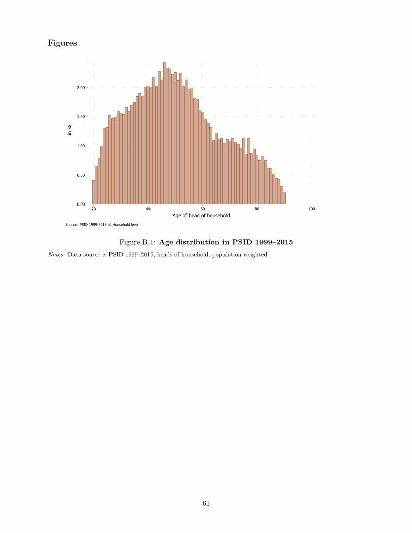
Figures

0.00

0.50

1.00

1.50

2.00

2.50

in %

20 40 60 80 100

Age of head of household

Source: PSID 1999-2015 at Household level

Figure B.1: Age distribution in PSID 1999–2015Notes: Data source is PSID 1999–2015, heads of household, population weighted.

61

Tables

Table B.1: Summary statistics PSID 1999–2015

(1) (2)1999-2015 1999-2015: HH-Headsmean/sd mean/sd

Calendar year 2004.143 2004.143(3.401) (3.401)

Age of head of household 46.067 46.067(15.851) (15.851)

Female 0.290 0.290(0.454) (0.454)

Married 0.519 0.519(0.500) (0.500)

Number of Years of Education 12.738 12.738(2.546) (2.546)

Individual labor earnings in $1,000 43.586 43.586(54.832) (54.832)

Labor income HH in $1,000 60.560 60.560(67.985) (67.985)

Pre-government HH income in $1,000 66.260 66.260(68.995) (68.995)

HH Wealth excl. equity (2016 USD 1,000) 94.590 94.590(160.661) (160.661)

HH Wealth incl. equity (2016 USD 1,000) 108.648 108.648(183.281) (183.281)

Self-Rated Health Status 2.442 2.442(1.080) (1.080)

No high school degree 0.187 0.187(0.390) (0.390)

High school degree 0.368 0.368(0.482) (0.482)

College 0.196 0.196(0.397) (0.397)

Insured 0.916 0.916(0.277) (0.277)

Head of HH 1.000 1.000(0.000) (0.000)

Observations 36643 36643Note: Unweighted sample statistics.

Notes: Unweighted summary statistics of heads of households based on PSID 1999–2015.

62