helsinki university of technologyFaculty of Electronics, Communications and Automation

Juhamatti Nikander

Induction Motor Parameter Identification in Elevator Drive Modernization

Thesis submitted for examination for the degree of Master of Science inTechnology

Espoo 7.1.2009

Thesis supervisor:

Prof. Jorma Luomi

Thesis instructor:

M.Sc. Lauri Stolt

helsinki university of technology abstract of themaster’s thesis

Author: Juhamatti Nikander

Title: Induction Motor Parameter Identification in Elevator DriveModernization

Date: 7.1.2009 Language: English Number of pages: 10+68

Faculty: Faculty of Electronics, Communications and Automation

Professorship: Electric Drives Code: S-81

Supervisor: Prof. Jorma Luomi

Instructor: M.Sc. Lauri Stolt

A study is presented where an induction motor, whose rotor is not allowed torotate, is identified using system identification methods based on transient andfrequency response tests. Precise control of elevators powered with frequencyconverter fed induction motors depends on the accuracy of the parameters used inthe motor controller, particularly when no external position or speed sensors areused. When an elevator is modernized with a new control system, the old motorcannot be identified with a regular locked rotor and no-load tests as the motoris not allowed to rotate. However, the identification can be performed in suchconditions by analyzing the voltages and currents when the motor windings areexcited with such an AC or DC that does not produce torque. A step responsemethod is introduced for the DC excitation where the desired motor parametersare obtained as a result when the measured data is processed with state variablefilters, and the produced linear system of equations is solved with a recursive least-squares algorithm. The frequency response method presented uses both DC andAC excitation. The method is based on finding the amplitude ratio and the phasedifference between the voltage and current phasors using the properties of theFourier series. This information is then used to calculate the inductance betweenthe motor terminals, from which the other motor parameters can be solved. Bothmethods are tested with simulations and experiments. The final choice of theproper identification method is found to be a compromise between the parameteraccuracy and measurement time.

Keywords: Elevator, induction motor, self-commissioning, parameter identifi-cation, standstill, step response, frequency response, state variablefiltering, recursive least-squares

teknillinen korkeakoulu diplomityontiivistelma

Tekija: Juhamatti Nikander

Tyon nimi: Oikosulkumoottorin parametrien identifionti hissikaytonmodernisoinnissa

Paivamaara: 7.1.2009 Kieli: Englanti Sivumaara: 10+68

Tiedekunta: Elektroniikan, tietoliikenteen ja automaation tiedekunta

Professuuri: Sahkokaytot Koodi: S-81

Valvoja: Prof. Jorma Luomi

Ohjaaja: Dipl.Ins. Lauri Stolt

Tassa tyossa tutkitaan, miten oikosulkumoottorin sahkoiset parametrit voidaanidentifioida askel- ja taajuusvastemenetelmien avulla pyorittamatta roottoria.Oikosulkumoottoria voimanlahteena kayttavien hissien ohjaustarkkuus riippuupitkalti siita, miten tarkasti taajuusmuuttajan momentti- ja nopeussaatajanparametrit vastaavat todellisia varsinkin, jos hissin paikkaa tai nopeutta ei mi-tata. Vanhojen hissien modernisoinnin yhteydessa ongelmaksi muodostuu se,etta olemassa olevaa moottoria ei voi identifioida perinteisilla oikosulku- jatyhjakayntikokeilla, koska moottoria ei voi pyorittaa kuormattomana. Sen si-jaan identifiointi voidaan tehda analysoimalla vaihejannitteita ja -virtoja, joitaesiintyy, kun staattorikaamityksiin syotetaan sellainen herate, joka ei aiheutapyorivaa sahkomagneettista kenttaa eika siten vaantomomenttia. Esitettavassaaskelvastemenetelmassa moottoria syotetaan tasavirtapulsseilla, jolloin halututparametrit saadaan, kun vaihejanniteen ja -virran mittaukset prosessoidaan tila-muuttujien suodatuksella ja saatu lineaarinen yhtaloryhma ratkaistaan rekursii-visella pienimman neliosumman algoritmilla. Toisessa, taajuusvasteeseen perustu-vassa, menetelmassa moottoria syotetaan yhta aikaa seka tasa- etta vaihtovirralla.Talloin moottorin parametrit voidaan ratkaista vaihejannitteen ja -virran valisenamplitudisuhteen ja vaihe-eron perusteella lasketun moottorin liittimista nakyvaninduktanssin taajuusriippuvuuden avulla. Molempia menetelmia on tutkittu sekatietokonesimuloinneilla etta kokeellisilla menetelmilla. Tulosten perusteella havait-tiin valitun menetelman olevan kompromissi parametrien tarkkuuden ja testinsuoritusajan valilla.

Avainsanat: Hissikaytto, oikosulkumoottori, parametrien identifiointi, askel-vaste, taajuusvaste, tilamuuttujien suodatus, rekursiivinen pieninneliosumma

iv

Acknowledgements

This Master’s thesis has been carried out for the R&D drive team of the elevatorcorporation Kone at Hyvinkaa, Finland. I would like to thank the team leader, JariHelvila, for providing this challenging and interesting subject available, and the chiefdesign engineer, Tuukka Kauppinen, for bringing this subject to my attention.

I wish to express my gratitude to the personnel in the Electric Drives Group ofHelsinki University of Technology: my supervisor, Professor Jorma Luomi, for thesubstantial guidance and support given in scientific writing, and for the valuableopinions expressed during the year. Special thanks go to Dr. Marko Hinkkanen forproviding initial literature on the subject, and for pointing out valuable comments.

I want to thank my instructor, M.Sc. Lauri Stolt, for the interest shown towards thesubject and for the practical tips given in the many educational discussions we had.I also appreciated the support provided on programming, proofreading and teachingdrive electronics.

I would also like to thank the drive specialists, Esa Putkinen, Risto Jokinen andPekka Hytti, for the professional comments and advice given regarding electronicsused in elevator drives. Furthermore, I wish to thank the other members of the driveteam and other people at Kone not mentioned here for providing the most friendlyworking environment.

Finally, I would like to thank my family for the love and support they have beengiving during the years of my studies.

Otaniemi, 7.1.2009

Juhamatti Nikander

v

Contents

Abstract ii

Abstract (in Finnish) iii

Acknowledgements iv

Contents v

Symbols and Abbreviations vii

1 Introduction 1

1.1 Objectives and Scope . . . . . . . . . . . . . . . . . . . . . . . . . . . 2

1.2 Structure . . . . . . . . . . . . . . . . . . . . . . . . . . . . . . . . . 3

2 Elevator Drive 4

2.1 Elevator Mechanics . . . . . . . . . . . . . . . . . . . . . . . . . . . . 4

2.2 Frequency Converter . . . . . . . . . . . . . . . . . . . . . . . . . . . 6

3 Induction Motor Theory 11

3.1 Structure and Operating Principle . . . . . . . . . . . . . . . . . . . . 11

3.2 Electrical Model . . . . . . . . . . . . . . . . . . . . . . . . . . . . . . 12

3.3 Mechanical Model . . . . . . . . . . . . . . . . . . . . . . . . . . . . . 17

4 Motor Control 18

4.1 Rotor Field Orientation . . . . . . . . . . . . . . . . . . . . . . . . . 19

4.2 Controller Detuning Effects . . . . . . . . . . . . . . . . . . . . . . . 20

5 Motor Identification Methods 22

5.1 Motor Name-plate . . . . . . . . . . . . . . . . . . . . . . . . . . . . 22

5.2 Stator Resistance Measurement . . . . . . . . . . . . . . . . . . . . . 25

5.3 Locked Rotor and No-load Tests . . . . . . . . . . . . . . . . . . . . . 27

5.4 Standstill Identification . . . . . . . . . . . . . . . . . . . . . . . . . . 30

5.5 Literature Review on Standstill Identification Methods . . . . . . . . 35

5.6 Step Response Identification . . . . . . . . . . . . . . . . . . . . . . . 37

5.7 Identification with State Variable Filtering . . . . . . . . . . . . . . . 40

vi

5.8 Frequency Response Identification . . . . . . . . . . . . . . . . . . . . 44

5.9 Magnetizing Curve Identification . . . . . . . . . . . . . . . . . . . . 48

6 Simulation Results 51

7 Experimental Results 57

8 Conclusions 60

References 62

A Linear Regression 67

vii

Symbols and Abbreviations

ai, bi coefficients of ith terms in polynomials U(s) and Y (s)B viscous damping coefficientBe B of the motor shaftBl B of the load reduced to the secondary wheelf0 low-pass filter cut-off frequencyf1 stator frequencyf2 slip frequencyfs sampling frequencyfsw switching frequencygi intermediate result in RLS algorithmh sampling periodI identity matrixIac alternating currentIdc direct currentIs0 stator no-load currentimec gear transmission ratioJe inertia of the motor shaftJl inertia of the load reduced to the secondary wheelk discrete time unitKl torsional spring coefficients reduced to the secondary wheelK(ω1) system gainl number of cycles measured during tmLD dynamic magnetizing (mutual) inductanceLe effective stator inductanceLm magnetizing (mutual) inductanceLM transformed magnetizing (mutual) inductanceLr, Ls rotor and stator self-inductancesLrσ, Lsσ rotor and stator leakage inductancesLσ total leakage inductancema, mf amplitude and frequency modulation ratiosN number of measurement pointsp number of pole pairsP covariance matrixPCur, PCus resistive power losses in rotor and statorPFer, PFes iron losses in rotor and statorPfr friction lossespij element in P on ith row and jth columnPin active three-phase input powerPin0, Pink no-load and short-circuit input powersPout mechanical output powerPstr stray lossesPwi windage lossesQ0 no-load Qin

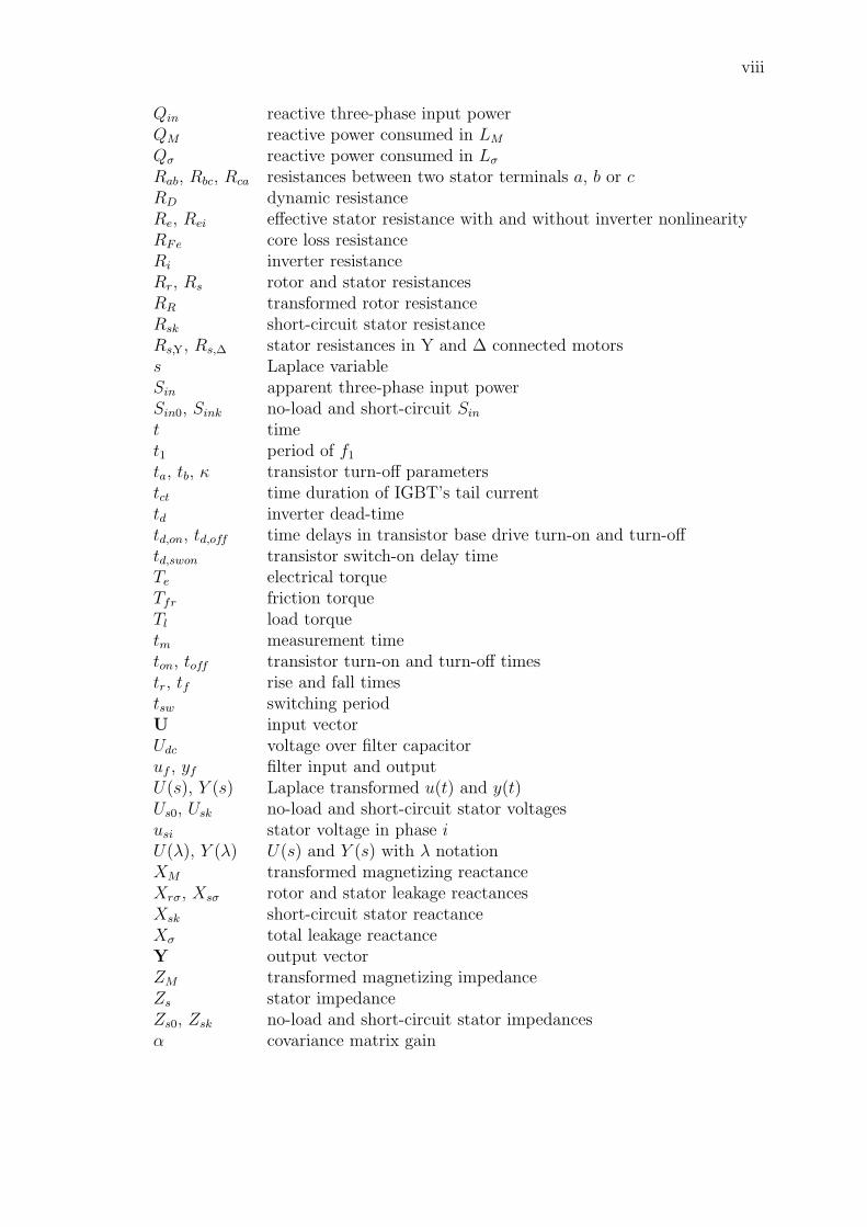
viii

Qin reactive three-phase input powerQM reactive power consumed in LMQσ reactive power consumed in LσRab, Rbc, Rca resistances between two stator terminals a, b or cRD dynamic resistanceRe, Rei effective stator resistance with and without inverter nonlinearityRFe core loss resistanceRi inverter resistanceRr, Rs rotor and stator resistancesRR transformed rotor resistanceRsk short-circuit stator resistanceRs,Y, Rs,∆ stator resistances in Y and ∆ connected motorss Laplace variableSin apparent three-phase input powerSin0, Sink no-load and short-circuit Sint timet1 period of f1

ta, tb, κ transistor turn-off parameterstct time duration of IGBT’s tail currenttd inverter dead-timetd,on, td,off time delays in transistor base drive turn-on and turn-offtd,swon transistor switch-on delay timeTe electrical torqueTfr friction torqueTl load torquetm measurement timeton, toff transistor turn-on and turn-off timestr, tf rise and fall timestsw switching periodU input vectorUdc voltage over filter capacitoruf , yf filter input and outputU(s), Y (s) Laplace transformed u(t) and y(t)Us0, Usk no-load and short-circuit stator voltagesusi stator voltage in phase iU(λ), Y (λ) U(s) and Y (s) with λ notationXM transformed magnetizing reactanceXrσ, Xsσ rotor and stator leakage reactancesXsk short-circuit stator reactanceXσ total leakage reactanceY output vectorZM transformed magnetizing impedanceZs stator impedanceZs0, Zsk no-load and short-circuit stator impedancesα covariance matrix gain

ix

αi, βi coefficients of ith terms in polynomials U(λ) and Y (λ)γ update coefficient vectorγi update coefficient of ith parameterδ1 angle between real axes of phase a and synchronous frame dδr rotor angleηg gear efficiency when power flows to the motorηm gear efficiency when power flows to the loadθ parameter vectorθi ith model parameterλ Lambda operatorµ forgetting factorσ leakage factorτm mechanical time constantτr, τs rotor and stator time constantsτ ′s transient stator time constantϕ regression vectorΦ regression matrixϕ0, ϕk angle ϕ1 in no-load and short-circuit conditionsϕ1 angle between stator voltage and current phasorsω0 filter angular cut-off frequencyω1 stator angular frequencyω2 rotor (slip) angular frequencyΩl angular speed of the loadωr electrical angular speed of the rotorΩr mechanical angular speed of the rotor

Space Vectors

i0 no-load magnetizing currentiFe iron loss currentim magnetizing currentiM transformed magnetizing currentir, is rotor and stator currentsiR transformed rotor currentui inverter voltage dropus stator voltageus,ref reference stator voltageψm

main flux linkage

ψr, ψ

srotor and stator flux linkages

ψrσ

, ψsσ

rotor and stator leakage flux linkages

ψR

transformed rotor flux linkage

ψσ

total leakage flux linkage

x

Subscripts

a, b, c phase a, b or cd real part in synchronous reference frameN nominal valueq imaginary part in synchronous reference framer rotor quantitys stator quantityα real part in stator reference frameβ imaginary part in stator reference frame

Other Notations

x complex phasor or space vectorx derivative of x with respect to timex amplitude of xx estimate or measurement of xx vectorX matrixX root-mean-square quantity of xX(s) transfer function∆x difference xi+1 − xi[λix](t) i times filtered x(t)bxc the value of x rounded down to the closest integer

Abbreviations

AC alternating currentCMFR correlation method of frequency responseDC direct currentDTC direct torque controlIGBT insulated gate bipolar transistorFD frequency domainFIR finite impulse responseFR frequency responseIIR infinite impulse responseLRNL locked rotor and no-loadLS least-squares algorithmPI proportional-integralRLS recursive least-squaresRMS root-mean-squareSR step responseSSFR standstill frequency responseSVF state variable filteringTD time domain

1 Introduction

Three-phase induction motors have been used widely in elevator applications fordecades thanks to the motor’s relatively simple structure, maintenance free operationand ability to start directly from the supply network. However, such an on-linestarting consumes energy more than necessary, and the starts and stops becomejerky as the motor can only be controlled with switches and relays.

During the 1980s, analog motor control systems evolved, and frequency convertersbecame popular, enabling the use of drives with variable voltage and frequency,which improved the stopping accuracy of the elevator car and reduced overall en-ergy consumption. Ever since the microprocessors became available with reasonableprices in the 1990s, the scope has been on controlling the motor more smoothly andefficiently.

Recently, the first generation of elevators with drives using induction motors havebegun to reach the end of their lifespan increasing the market for elevator modern-ization. The idea is to replace the old and excessively worn parts of the drive withnew high-performance and high-efficiency components while trying to keep the oldmotor and gear in place to avoid increasing the costs too much.

However, the name-plates of the old, as well as the new, induction motors haveinsufficient information, if any, to be used with modern control methods. In addition,the motors used in elevator installations are most likely to be supplied by variousmanufacturers instead of being built by the one modernizing the elevator. In sucha case, a custom setup has to be carried out for the motor and drive electronics,which is a very time-consuming task and can only be performed by very experiencedpersonnel. Therefore, there is a need for a drive capable of self-commissioning, i.e.identifying the parameters of an unknown motor without user intervention.

Previously, induction motors have been identified by performing several tests duringwhich the rotor had to be kept locked mechanically or disconnected from the load,i.e. with the DC test, locked rotor test and no-load test. These restrictions causeproblems in elevator modernization for several reasons. Although the rotor couldbe locked mechanically with the motor brakes, there is no guarantee that the oldbrakes will be able to hold the full pull-up torque produced in the locked rotortest in addition to the torque caused by the load - the unbalanced elevator car andcounterweight. Of course, the torque could be produced into the direction oppositeto the one caused by the load, or the system could be balanced by adding weighseither to the elevator car or to the counterweight. However, the system would stillhave to be modified for the no-load test.

A better idea would be to remove the heavy flywheel from the motor shaft andthe mechanical coupling between the motor and the gear. However, the couplingcannot be removed without removing the brake arms, and doing so would cause thecounterweight to fall freely. Thus, it would be first necessary to remove the ropesfrom the traction sheave, a grooved pulley connected to the secondary wheel of thegear, but the ropes, in turn, cannot be removed without lowering the counterweight

2

to the bumper and without locking the elevator car. Thus, there is no practical wayof achieving the no-load conditions in any reasonable time.

1.1 Objectives and Scope

The objective of this Master’s thesis is to find the most suitable identification methodfor the electrical parameters of a typical induction motor used in elevator applica-tions. The following restrictions must be obeyed:

The rotor is not allowed to rotate nor produce torque.

The motor is supplied with a frequency converter where the stator voltagesare not measured.

The existing hardware must not be changed.

The parameters should be accurate enough to be used in a modern speedsensorless vector control.

Luckily, the electrical parameters can be identified without rotating the motor at allif the stator windings are fed with an excitation that does not produce a rotatingelectromagnetic field, i.e. if the motor is controlled as if two of the three stator phaseswere connected to the frequency converter and the third one left connected, or as ifthe two phases were connected in parallel, and the resulting equivalent winding inseries with the third one. With such an excitation, no torque is produced, and thereis no need to lock the rotor nor disconnect the load.

Unfortunately, this type of standstill identification is not a very easy task to do asthe identified system is far from being ideal due to the nonlinearities present in thefrequency converter and in the induction motor itself. For example, the frequencyconverter’s output voltage depends nonlinearly on the motor’s phase currents be-cause dead-time is added to the transistor switch-on delays. Moreover, the outputvoltage depends on the forward voltage drops of the used power devices, particu-larly when the output voltage is low. On the other hand, inductances formed by thestator windings and the rest of the magnetic circuit depend on the direction and themagnitude of the current due to hysteresis and saturation. Furthermore, the rotorresistance and leakage inductance change with stator frequency due to the skin andproximity effects. In addition, the iron losses dissipated in the motor core dependon that frequency.

The studied identification methods are divided into step and frequency responsemethods. In the former, the stator windings are supplied with either voltage orcurrent steps, and the resulting current or voltage is measured, after which the mea-sured data is fitted to the one calculated from the motor model. The fitting becomespossible if at least two measurements are gathered. In practice, the data is fittedwith linear regression, reducing the effects of noise and single wrong measurements.

3

As a result, a parameter vector is obtained, from which the motor parameters canbe calculated.

In the frequency response methods, the stator windings are supplied with sinusoidalvoltages of constant amplitudes and frequencies. Furthermore, a DC current isused to set the correct level of magnetization and to reduce the effect of hysteresis.The measurements are taken from the current response after the initial transientshave decayed. The idea is to calculate the amplitude ratio and phase differencebetween the fundamental voltage and current phasors. This information is thenused to calculate the effective input inductance seen from the motor terminals atthe frequencies of interest, after which the other motor parameters can be calculatedfrom that inductance.

1.2 Structure

The contents of this thesis are organized in the following way. After this introduction,the following two chapters, 2 and 3, introduce mathematical models for a simpleelevator, frequency converter and induction motor. In Chapter 4, motor controlbased on space vector theory is briefly reviewed, after which controller detuningeffects are discussed.

The main subject of this thesis begins in Chapter 5 where the first section explainsinformation that can be derived from the motor name-plate, and the second sectiondiscusses the problems that occur when winding resistances are measured with afrequency converter. Then, the locked rotor and no-load tests are presented, followedby a derivation of the model used in standstill identification. A literature review ispresented in the middle of the chapter, and the remaining parts show how the motoris identified using the step and frequency response methods.

In the next two chapters, 6 and 7, different identification methods are studied withcomputer simulations and experimental tests. Finally, the thesis is concluded inChapter 8.

4

2 Elevator Drive

The first section of this chapter describes a construction of a simple elevator andintroduces a mathematical model for the mechanical dynamics, after which the struc-ture and behavior of the elevator power supply, a frequency converter, is explained.

2.1 Elevator Mechanics

A simple elevator consists of a shaft, car, counterweight, ropes, a number of tractionsheaves: pulleys with multiple grooves; bumpers, a motor and, possibly, a reductiongear, and necessary safety equipment. The shaft has guide rails on the walls, alongwhich the car and the counterweight move vertically. Usually, the motor lies inits own machine room at the top of the shaft. The motor shaft is connected tothe reduction gear or directly to the driving traction sheave, whose purpose, inaddition to transforming rotation to transversal motion, is to add more friction tothe ropes. The shaft, car and counterweight all have a number of deflector sheaves,whose purpose is to pass the ropes, connecting the car and counterweight alongthe sheaves, to a particular direction. With multiple ropes and deflector sheaves,forces acting on individual ropes can be reduced. The amount of this reductionis characterized by the roping factor. Any other roping than 1:1 causes the ropesto move faster than the elevator car. Therefore, the roping as well acts as a gear.The bumpers are placed at the bottom of the shaft, where they act as ultimateboundaries, against which the car and the counterweight will be stopped if othersafety equipment fail to operate.

Dynamic Model

Modeling mechanical elevator dynamics is a very difficult task as the real elevatorsystem has a vast number of moving parts with unknown parameters. However, asimple dynamic model can be built for simulation and model parameter verificationpurposes. The considered system in Figure 2.1 consists of two moments of inertia– one inertia Je for the motor shaft and the other Jl for the rest of the movingelevator parts – connected to each other with a reduction gear. Frictions in themotor and gear, and the elevator are modeled with two viscous dampers Be andBl, respectively, and the oscillatory behavior, caused by the flexible ropes, with onetorsional spring constant Kl. The gear is thought to be ideal, i.e. no backlash andunity efficiency. As such, the equations of motion are

JedΩ1(t)

dt= Te(t)−BeΩ1(t)− T1(t) (2.1a)

dT2(t)

dt= Kl

[Ω2(t)− Ωl(t)

](2.1b)

JldΩl(t)

dt= T2(t)−BlΩl(t)− Tl(t) (2.1c)

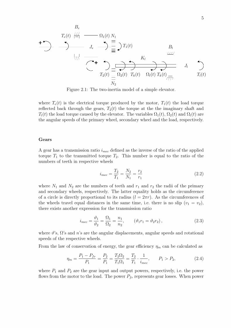
5

Te(t)

Be

Je

Ω1(t)

T1(t)

N1

N2

T2(t) Ω2(t) Tk(t) Ωl(t) Tk(t)

Kl

Bl

Jl

Tl(t)

Figure 2.1: The two-inertia model of a simple elevator.

where Te(t) is the electrical torque produced by the motor, T1(t) the load torquereflected back through the gears, T2(t) the torque at the the imaginary shaft andTl(t) the load torque caused by the elevator. The variables Ω1(t), Ω2(t) and Ωl(t) arethe angular speeds of the primary wheel, secondary wheel and the load, respectively.

Gears

A gear has a transmission ratio imec defined as the inverse of the ratio of the appliedtorque T1 to the transmitted torque T2. This number is equal to the ratio of thenumbers of teeth in respective wheels

imec =T2

T1

=N2

N1

=r2

r1

(2.2)

where N1 and N2 are the numbers of teeth and r1 and r2 the radii of the primaryand secondary wheels, respectively. The latter equality holds as the circumferenceof a circle is directly proportional to its radius (l = 2πr). As the circumferences ofthe wheels travel equal distances in the same time, i.e. there is no slip (v1 = v2),there exists another expression for the transmission ratio

imec =ϑ1

ϑ2

=Ω1

Ω2

=n1

n2

, (ϑ1r1 = ϑ2r2) , (2.3)

where ϑ’s, Ω’s and n’s are the angular displacements, angular speeds and rotationalspeeds of the respective wheels.

From the law of conservation of energy, the gear efficiency ηm can be calculated as

ηm =P1 − Pfr

P1

=P2

P1

=T2Ω2

T1Ω1

=T2

T1

· 1

imec, P1 > P2, (2.4)

where P1 and P2 are the gear input and output powers, respectively, i.e. the powerflows from the motor to the load. The power Pfr represents gear losses. When power

6

flows from the load to the motor, the latter working as a generator, the efficiency ηgis defined as

ηg =P2 − Pfr

P2

=P1

P2

=T1Ω1

T2Ω2

=T1

T2

imec, P1 < P2. (2.5)

With the gear transmission ratio defined above, and noting that T1 = Te and Ω1 =Ωr, the variables T1, T2, Ω1 and Ω2 can be removed from Equation (2.1) yielding astate space form

x1(t) =

Ωr(t)

Te(t)

Ωl(t)

=

−Be/Je −1/Je 0Kl/i

2mec 0 −Kl/imec

0 imec/Jl −Bl/Jl

Ωr(t)Te(t)Ωl(t)

+

1/Je 00 00 −1/Jl

[Te(t)Tl(t)

]= A1x1(t) + B1u1(t). (2.6)

For control purposes, the actual use of this model is rather limited as it involvesmeasuring the torque and the angular speed of the primary shaft with an expensivetorque sensor and a tachometer. Therefore, the main purpose of this model is tosimulate the pulsating load torque caused by flexible ropes.

For better dynamics, the model could be extended with less simplified elevator dy-namics containing two dynamic masses for modeling the inertia of the car, coun-terweight and ropes and two viscous dampers and linear springs for modeling theflexibility of the ropes and other two viscous dampers for the car and counterweight.This less simplified model yields a fifth- to seventh-order model for the elevator dy-namics and a third-order model for the motor dynamics. This thesis considers onlythe motor part. For more detailed modeling of elevator mechanics, the interestedreaders could refer to the Master’s thesis by Salomaki (2003) and its references.

2.2 Frequency Converter

A frequency converter is a power electronics device that converts power from a supplynetwork to a load with controllable amplitude and frequency. A schematic diagramof one topology of frequency converters used in elevator drives is shown in Figure2.2. It consists of a three-phase, six-pulse, full-bridge diode rectifier (1), a brakechopper (2), a large filter capacitor (3) and a three-phase pulse-width-modulatedvoltage-source inverter (4). Measurements are taken from the voltage over the filtercapacitor and from the currents of two output phases.

The first part rectifies the supply AC voltage into DC over the filter capacitor withthe voltage given on average by

Udc =3

π

√2Un ≈ 1.35 · Un (2.7)

where Un is the supply network phase-to-phase voltage (Mohan et al., 2003). Due tothe finite interval needed by current commutation between the conducting diodes,

7

(1) (2) (3) (4)

RST

a b c

N

Figure 2.2: A typical frequency converter.

the DC side voltage (2.7) is reduced by

∆Udc =3

πωnLkIdc = 6fnLkIdc (2.8)

where ωn = 2πfn is the angular frequency of the supply and Lk the short-circuitinductance of the supply network at the frequency converter’s input terminals. Thecurrent Idc is the current on the DC side.

The brake chopper is used to avoid voltage increase in the filter capacitor by dissi-pating the excess energy in the braking resistors when the power flows from the loadto the supply, i.e. when the motor is braking or acting as a generator, and whenthe frequency converter is equipped with a diode-rectifier, which is not capable ofconverting this energy back to the supply.

The purpose of the PWM inverter is to create voltages with controllable magnitudeand frequency. The inverter consists of three ’legs’, each having two pairs of tran-sistors and diodes, the upper and lower ones. The transistors in each one of theseinverter-legs are controlled in a complementary fashion, i.e. one transistor conductsat a time, to avoid short-circuiting the filter capacitor.

The instantaneous inverter output voltages with respect to the assumed three-phaseload neutral point are

usa =2

3uaN −

1

3(ubN + ucN) (2.9a)

usb =2

3ubN −

1

3(uaN + ucN) (2.9b)

usc =2

3ucN −

1

3(uaN + ubN) (2.9c)

where uiN , i ∈ a, b, c , are the amplitudes of the inverter output voltages withrespect to the negative DC-bus.

When pulse-width modulation based on suboscillation method is used, the aver-age inverter output voltage and frequency are characterized by the amplitude and

8

frequency modulation ratios ma and mf , respectively,

ma =uctrlutri

mf =fswf1

(2.10)

where uctrl is the control signal used for modulating the duty ratio of the transis-tors, and f1 the fundamental frequency of the control signal and the desired outputvoltage. The voltage utri is the amplitude of the carrier signal whose frequency fswis also the transistor switching frequency.

The fundamental-frequency phase-to-neutral voltage has, on average, an amplitude

us = maUdc2

(2.11)

providing that the modulator operates in the linear region, i.e. ma ≤ 1.0. Accordingto Holtz (1994), the voltage can be increased if third harmonics are added to thecontrol signals uctrl. For example, if 16.7% of third harmonic is added, Equation(2.11) can be replaced with

us :=2√3us = ma

Udc√3≈ 0.577 ·maUdc. (2.12)

Dead-time

In practice, the obtained output voltage is reduced due to the added transistor dead-time (blanking time), during which none of the two transistors in one of the threeinverter-legs are conducting to avoid short-circuiting the filter capacitor. Thus, theoutput voltage floats and is characterized by the magnitude and the direction of theload current is and, therefore, on the load’s displacement power factor cosϕ1 as well.

According to Ruff and Grotstollen (1996), the dead-time is defined as the differencebetween the switch-on delay time td,swon of the non-conducting transistor and theturn-off time toff (is) of the conducting one

td(is) = td,swon − toff (is). (2.13)

If the current rise and fall times, tr and tf , and the base drive turn-on and turn-offdelays, td,on and td,off , are taken into account, the definition becomes

td(is) = td,swon + td,on − td,off (is)− tf (is). (2.14)

Figure 2.3 illustrates the case. The dead-time is chosen conservatively as it is difficultto estimate the current tail time tct present in some transistor types, for example,in insulated-gate bipolar transistors.

There exists several methods for compensating errors in the output voltage causedby the dead-time varying from the simplest averaging methods to model-referenceadaptive control methods. One interesting method is the pulse-based dead-time

9

td

td,on

ton

td,off

toff

trtf tct

td,swon

iT+(t) iT−(t)iD+(t)ia(t)

t

Figure 2.3: Diode-IGBT current switching characteristics for one inverter-leg, ac-cording to Martin (1996). T+ refers to the upper and T− to the lower transistor andD+ is the freewheeling diode of the upper transistor.

compensation, which has an ability to reconstruct the magnitude and phase of theoutput voltage as if the dead-time was not generated at all (Leggate and Kerkman,1997).

In addition to the nonlinear inverter voltage drop, the output voltage is reducedby the voltage drops over the power transistors, the freewheeling diodes and themotor cabling. Therefore, the output voltage differs from the commanded voltage,which imposes problems in motor identification as the phase voltages are not directlymeasured. Instead, the output voltages are estimated from the modulation index ma

and the measured DC filter capacitor voltage as in Equation (2.11). The followingarticles provide a good starting point for a study of methods used for compensatingdifferent inverter nonlinearities: (Blaabjerg and Pedersen, 1994), (Choi and Soul,1994), (Munoz and Lipo, 1999) and (Urasaki et al., 2005).

Current Measurement

The situation is a bit easier for the motor currents as two of the three phase currentsare measured and the third one can be calculated as a linear combination of the firsttwo

isa(t) + isb(t) + isc(t) = 0. (2.15)

The phase currents are usually filtered in hardware before being measured. Thus,the obtained currents are delayed versions of the real ones as can be observed from

10

us,ref

us

isis,m ω1

ϕPWM

ϕ1

ϕm

Figure 2.4: Vector diagram of the inverter output voltage and current. us,ref is thecommanded voltage and is,m the measured current. The angles ϕPWM and ϕm areexaggerated for clarity.

the vector diagram in Figure 2.4.

The magnitude and phase errors caused by the filter can easily be compensated insoftware. For example, if the output current is filtered with a first-order low-passfilter

Gf (jω) =ω0

ω0 + jω(2.16)

where ω0 is the filter bandwidth, the magnitude and phase of the filter output canbe obtained from

|Gf (jω)| = 1√1 +

(ω

ω0

)2(2.17a)

ϕm = − arctan

(ω

ω0

). (2.17b)

11

3 Induction Motor Theory

In this chapter, the structure of the induction motor is explained followed by areview of the equations characterizing its electrical and mechanical behavior.

3.1 Structure and Operating Principle

The induction motor consists of a round and hollow static part with a cylindricalrotating part inside of it. The former is referred to as the stator and the latteras the rotor. The stator core has slots inside of its inner surface and the rotorinside of its outer surface. The stator slots of a three-phase motor contain threesets of windings each separated by 120 electrical degrees, whereas the rotor slotscontain conducting bars enclosed by short-circuit rings at both ends. A motor witha rotor circuit of this type is called a squirrel-cage induction motor. An alternativeconfiguration is the slip-ring induction motor, whose rotor winding is connected toslip-rings at the motor shaft, from which it is possible to connect the rotor windingto external resistors or to a frequency converter. The stator and rotor cores aremade of high-permeability materials to achieve small reluctances in the path of themagnetic fluxes, which is needed to produce maximal magnetic flux with minimalmagnetizing current. The mutual inductance between the stator and rotor windingsis characterized by the width of the air gap – the smaller the gap, the greater theinductance. On the other hand, the stator and rotor leakage inductances are mainlydetermined by the shape of the respective windings and slots.

When the stator windings are fed with symmetric sinusoidal voltages whose angularfrequency is ω1, the resulting currents create a rotating magnetic field in the magneticcircuit formed by the stator and rotor cores and the air gap between them. The fieldrotates at a geometrical angular frequency

Ωg =ω1

p(3.1)

where the parameter p is the number of pole pairs formed by the stator windings.This rotating magnetic field induces electromotive forces (emf) in the closed rotorcircuit. The currents caused by these emfs produce a magnetic field opposing therotating stator field. Now, according to Lenz’s law, a force will act on a current-carrying conductor placed in a magnetic field. Thus, the rotor bars will be pushedby a tangential magnetic force, producing electrical torque with respect to the rotorshaft. The rotor begins to rotate if the electrical torque is not balanced by an oppo-site mechanical torque, which further means that the rotor will not rotate exactlyat the same, synchronous, angular speed Ωg as the stator field does. Instead, therotor will start to rotate asynchronously with a mechanical angular speed

Ωr =ωrp

=ω1 − ω2

p(3.2)

12

α

β d

q

δr = ωr

δr

δ1

Figure 3.1: Stator and synchronous coordinate axes.

where ωr is the electrical angular speed of the rotor and ω2 the angular slip frequency.More detailed explanation of the motor structure and operating principle can befound in (Sadarangani, 2000) and (Krishnan, 2001).

3.2 Electrical Model

The induction motors considered in this thesis have three-phase stator windings.Voltages, currents and flux linkages in such a three-phase system are compactlydescribed by space vectors, which were first proposed in 1959 by Kovacs and Raczaccording to Holtz (1995). A general space vector is defined as a complex variable

xs(t) = xα(t) + jxβ(t) =2

3

[xa(t) + ej2π/3xb(t) + e−j2π/3xc(t)

](3.3)

where the quantities in the three phases are denoted by the subscripts a, b and c.The space vector maps a three-phase system into a two-phase system with α and βcoordinate axes as is illustrated in Figure 3.1. The stator reference frame is fixed tothe αβ axes. The other coordinate system used, in the soon to be introduced modelof induction motor, is the synchronous reference frame with d and q coordinate axes.The subscript d stands for direct and q for quadrature. The synchronous referenceframe rotates with the angular frequency of the stator current. Transformationbetween the two coordinate systems is defined as

x(t) = xd(t) + jxq(t) = e−jδ1xs(t) (3.4)

13

where the transformation angle δ1 is defined as

δ1 =

∫ω1dt. (3.5)

The synchronous reference frame is used because all control signals that vary sinu-soidally in the stator reference frame became constants. Consequently, such signalscan easily be controlled with regular proportional-integral (PI) controllers withoutsteady-state error.

As zero-sequence components cannot be described with space vectors, such compo-nents have to be handled separately as the averages in the three phases

x0(t) =1

3[xa(t) + xb(t) + xc(t)] . (3.6)

All variables defined in the stator reference frame are denoted by right superscripts s.For the synchronous reference frame the superscripts are omitted. The superscriptsare also omitted if the motor does not rotate, in which case both reference framesare equal.

T Equivalent Circuit

The induction motor resembles a transformer whose secondary winding is free tomove; therefore, it has almost same equivalent circuit, Figure 3.2, with only a slightchange caused by the rotor-emf jωrψ

s

r. The stator and rotor voltage equations for

the induction motor with a squirrel-cage rotor are

dψss

dt= uss −Rsi

ss (3.7a)

dψsr

dt= jωrψ

s

r−Rri

sr (3.7b)

where ψss

and ψsr

are the stator and rotor flux linkages, Rs and Rr the stator androtor resistances, respectively. The flux linkages are defined as

ψss

= ψssσ

+ ψsm

(3.8a)

ψsr

= ψsrσ

+ ψsm

(3.8b)

ψssσ

= Lsσiss (3.8c)

ψsrσ

= Lrσisr (3.8d)

ψsm

= Lmism (3.8e)

where ψsm

, ψssσ

and ψsrσ

are the main flux linkage and the stator and rotor leakageflux linkages, respectively. Lm, Lsσ and Lrσ are the magnetizing inductance and thestator and rotor leakage inductances, correspondingly. The magnetizing current ismis the sum of the stator and rotor currents, iss and isr, if the core loss current isFe

14

and resistance RFe are neglected as they usually are, particularly if the motor is notoperated with field-weakening (Levi et al., 1996). All rotor variables are reduced tothe stator-side.

For control purposes, it is useful to take the stator current and the rotor flux linkageas the state variables as most frequency converters have a closed-loop current controlwhose current measurements can be used, and because the rotor flux linkage can beestimated (Holtz, 1995). With this choice, Equations (3.7) become(

Ls −L2m

Lr

)dissdt

= uss −(Rs +Rr

L2m

L2r

)iss +

(Rr

Lr− jωr

)LmLr

ψsr

(3.9a)

dψsr

dt= Rr

LmLr

iss −(Rr

Lr− jωr

)ψsr

(3.9b)

where the stator and rotor self-inductances, Ls = Lm + Lsσ and Lr = Lm + Lrσ,have been used.

Inverse-Γ Equivalent Circuit

In the inverse-Γ model of Figure 3.3, the rotor leakage inductance is transformedto the stator side and combined with the stator leakage inductance to form a totalleakage inductance Lσ. This choice reduces the number of parameters by one, andis thus more suitable for control purposes and motor identification as the individualleakage inductances have little effect on motor control.

From Equations (3.9), the transformed rotor variables and parameters can be defined

ψsR

=LmLr

ψsr

(3.10)

isR =LrLm

isr (3.11)

isM = iss + isR (3.12)

LM =L2m

Lr(3.13)

Lσ = Ls − LM (3.14)

RR =

(LmLr

)2

Rr (3.15)

where LM and RR are the transformed magnetizing inductance and rotor resistance,respectively.

These new definitions change the stator and rotor flux linkages (3.8) to

ψss

= ψsσ

+ ψsR

(3.16a)

ψsσ

= Lσiss (3.16b)

ψsR

= LM isM (3.16c)

15

and the voltage equations (3.7) to

dψss

dt= uss −Rsi

ss (3.17a)

dψsR

dt= jωrψ

s

R−RRi

sR. (3.17b)

By substituting Equations (3.10)–(3.16) to the new voltage equations (3.17), thestate variable equations (3.9) transform to

Lσdissdt

= uss − (Rs +RR)iss +

(RR

LM− jωr

)ψsR

(3.18a)

dψsR

dt= RRi

ss −

(RR

LM− jωr

)ψsR. (3.18b)

In synchronous frame, the above equations are

Lσdisdt

= us − (Rs +RR + jω1Lσ)is +

(RR

LM− jωr

)ψR

(3.19a)

dψR

dt= RRis −

(RR

LM+ jω2

)ψR. (3.19b)

Steady State Inverse-Γ Equivalent Circuit

In steady state, the differential operators in Figure 3.3 can be replaced with jω1 ifsinusoidal input voltages and currents are being used. With some algebraic manip-ulations, Equation (3.17) transforms to

U ss = RsI

ss + jω1 (Lσ + LM) Iss + jω1LMI

sR (3.20a)

IsR = − jω1LMω1

ω2RR + jω1LM

Iss (3.20b)

where a symmetric three-phase supply is assumed with 120-degree phase shift be-tween respective voltages and currents. The phasor representation

U ss = Use

jω1t = Us∠0 (3.21a)

Iss = Isej(ω1t−ϕ1) = Is∠−ϕ1 (3.21b)

is used for sinusoidal variables. Figure 3.4 shows the corresponding equivalent circuitfor the steady state conditions.

Equation (3.20) suggests an expression for the motor impedance

Zss = Rs +

ω1LMω2τr

1 + (ω2τr)2 + jω1

[Lσ +

LM

1 + (ω2τr)2

]= Re + jω1Le (3.22)

where τr is the rotor time constant LM/RR, and Re and Le the effective statorresistance and inductance, respectively. From now on, the right superscript s isomitted in complex phasors.

16

biss-

isr A A A

Rs

Lsσ

ddt

Lrσ

ddt

rr is0?

isFe ? ism?

Lm

ddt

HHH

RFe

rrb

HHH

Rr

+

−jωrψ

s

r

uss

?

Figure 3.2: Dynamic T equivalent circuit.

biss-

isR A A A

Rs

Lσ

ddt

rr is0?

isFe ? isM?

LM

ddt

HHH

RFe

rrb

A A ARR

+

−jωrψ

s

Russ

?

Figure 3.3: Dynamic inverse-Γ equivalent circuit.

bIss-

IsR A A A

Rs

jω1Lσrr Is0?

IsFe? IsM?

jω1LM

HHH

RFe

rrb

HHH ω1

ω2

RRU ss

?

Figure 3.4: Steady state per-phase inverse-Γ equivalent circuit.

17

Electrical Power

The instantaneous apparent three-phase input power Sin(t) taken from the frequencyconverter or the supply network is defined as

Sin(t) =3

2uss(t)

(iss(t)

)∗= Pin(t) + jQin(t) (3.23)

and the active and reactive input powers, Pin(t) and Qin(t), as

Pin(t) = usa(t)isa(t) + usb(t)isb(t) + usc(t)isc(t) (3.24a)

=3

2

(usα(t)isα(t) + usβ(t)isβ(t)

)(3.24b)

Qin(t) =1√3

[usa(t)

(isc(t)− isb(t)

)+usb(t)

(isa(t)− isc(t)

)+usc(t)

(isb(t)− isa(t)

)](3.24c)

=3

2

(usβ(t)isα(t)− usα(t)isβ(t)

). (3.24d)

In steady state, the three-phase power is constant

Sin = |Sin| =√P 2in +Q2

in = 3UsIs =3

2

√(u2

sα + u2sβ)(i2sα + i2sβ) (3.25a)

Pin = 3UsIs cosϕ1 =3

2

(usαisα + usβisβ

)(3.25b)

Qin = 3UsIs sinϕ1 =3

2

(usβisα − usαisβ

)(3.25c)

where the parameter ϕ1 is the angle between the fundamental-frequency stator volt-age and current phasors.

3.3 Mechanical Model

The motor mechanics are given by the equation of motion

JedΩr(t)

dt= Te(t)− Tl(t) (3.26)

where the parameter Je is the system’s moment of inertia reduced to the rotor shaft.The variables, Te, and Tl, are the electrical torque produced by the motor and thetorque caused by the load.

The electrical torque is defined as

Te =3

2p Im

(ψs

R)∗iss

=

3

2p Im

ψ∗Ris

=

3

2p(ψRdisq − ψRqisd), (3.27)

which, for the control purposes, is given in the synchronous frame.

18

4 Motor Control

This chapter describes how the induction motor is controlled as a DC motor in thevector control scheme based on indirect rotor field orientation. The knowledge ofthis is necessary as it gives the means to understand how the motor behavior isaffected by the choice of incorrect controller parameters or by the deviations in theactual motor parameters. Other possible control methods are, e.g., the slip speedcompensated U/f -control, which is based on the steady state equations (Stolt, 2005);or the direct torque control (DTC), which is based on the hysteresis control of thestator flux linkage and the electrical torque (Harnefors, 2003).

The modern control system of an induction motor is based on previously introducedcomplex-valued electrical and mechanical differential equations (3.18) or (3.19) and(3.26). Those equations have to be separated into the real and imaginary parts sothat the motor can be controlled with a digital signal processor. The separationreveals a nonlinear and strongly cross-coupled system of equations

Lσdisd(t)

dt= usd(t)− (Rs +RR)isd(t) + Lσω1(t)isq(t)

+RR

LMψRd(t) + ωr(t)ψRq(t) (4.1a)

Lσdisq(t)

dt= usq(t)− (Rs +RR)isq(t)− Lσω1(t)isd(t)

+RR

LMψRq(t)− ωr(t)ψRd(t) (4.1b)

dψRd(t)

dt= RRisd(t)−

RR

LMψRd(t) + ω2(t)ψRq(t) (4.1c)

dψRq(t)

dt= RRisq(t)−

RR

LMψRq(t)− ω2(t)ψRd(t) (4.1d)

Jdωr(t)

dt=

3p2

2ψRd(t)isq(t)−

3p2

2ψRq(t)isd(t)− pTl(t). (4.1e)

The couplings between the different complex-valued first-order subsystems can beremoved as each system has its own dynamics given by the time constants τ ′s =Lσ/(Rs + RR), τr = LM/RR and τm = J/b for the stator current, rotor flux linkageand mechanical dynamics, respectively. The bandwidths of the subsystem dynamicsare separated, stator current dynamics being the fastest and mechanical the slowest,i.e. τ ′s τr τm. Therefore, each control loop can be designed independently.Figure 4.1 illustrates such a cascaded control system.

The couplings between the components of the stator current and the stator angularfrequency in Equations 4.1a and 4.1b are easily removed by subtracting the cor-responding products from the current controller’s output if only the total leakageinductance is known

usd(t) = u′sd(t)− Lσω1(t)isq(t) (4.2a)

usq(t) = u′sq(t) + Lσω1(t)isd(t) (4.2b)

19

θr,ref ωr,ref

isd,ref

isq,ref

us,refisa isc

ωr

δrFigure 4.1: Cascaded motor control system.

u′sd and u′sq are the current controller’s outputs. This choice reduces the statorcurrent dynamics to

Lσdisd(t)

dt= u′sd(t)− (Rs +RR)isd(t) +

RR

LMψRd(t) + ωr(t)ψRq(t) (4.3a)

Lσdisq(t)

dt= u′sq(t)− (Rs +RR)isq(t) +

RR

LMψRq(t)− ωr(t)ψRd(t). (4.3b)

But there still exists bilinear nonlinearities between the electrical angular speed ofthe rotor and the components of the rotor flux linkage. However, these couplingscan easily be removed by keeping the rotor flux linkage constant, or the term couldbe removed completely if the speed were measured, and the value of the magnetizinginductance were known.

4.1 Rotor Field Orientation

The rotor field orientation is the key in controlling the induction motor as a DCmotor. This orientation is obtained if the d-axis of the synchronous frame is fixedinto the direction of the rotor flux linkage

θ1 = argψsR. (4.4)

Thus, the rotor flux linkage becomes real-valued

ψR

= ψRd + jψRq = ψR. (4.5)

Such an orientation transforms the rotor flux linkage equations (4.1c) and (4.1d)into

dψR(t)

dt= RRisd(t)−

RR

LMψR(t) (4.6a)

ω2(t) = RRisq(t)

ψR(t)(4.6b)

which further reduce to

ψR = LM isd (4.7a)

ω2(t) =RR

ψRisq(t) (4.7b)

20

when the rotor flux linkage is kept constant. If the stator d-current and the angularslip frequency are controlled as the equations above suggest, the system (4.1a)–(4.1e)is simplified into a linear system resembling a DC-motor

Lσdisq(t)

dt= u′sq(t)− (Rs +RR)isq(t)− ψRωr(t) (4.8a)

Jdωr(t)

dt=

3

2p2ψRisq(t)− pTl(t). (4.8b)

It is observed that with proper rotor field orientation, the torque and speed cansimply be controlled with the stator q-voltage. Therefore, the control performancedepends on how accurately the magnitude and the direction of rotor flux linkagecan be estimated in Equation (4.4), which, on the other hand, depends on howaccurately the motor parameters are known.

4.2 Controller Detuning Effects

As was pointed out in the previous section, the drive performance depends on theuse of correct model parameters in the current, speed and position controllers. Un-fortunately, the motor parameters change heavily during operation as the statorand rotor resistances change with temperature whereas the leakage and magnetizinginductances change with the magnitude and the direction of the stator current, i.e.with the magnetic saturation and hysteresis of the iron core. Furthermore, the rotorparameters change with frequency due to the skin and proximity effects in the rotorbars. Moreover, the iron losses change with the stator frequency.

The total leakage inductance is one of the most important parameters in the in-duction motor control as it is used to decouple the control system. A wrong valuein the current controller causes pulsations in the produced torque when either thereference torque or rotor flux is changed.

On the other hand, the stator resistance is not that important in the RFO controlschemes, although, an incorrect value causes steady state error in the current re-sponse, and thus in the torque and rotor flux as well. The U/f method, however,is more sensitive to the stator resistance, particularly when operating with low fre-quency. The exact knowledge of the stator resistance is needed also in RFO schemesif the rotor speed is not measured but estimated. In general, the number and ac-curacy of parameters required increases when the number of sensors is reduced asmore variables need to be estimated.

The most important parameters in the RFO based motor control are the ones usedin estimating the direction of the rotor flux. The second most important parametersare the transformed rotor resistance and magnetizing inductance as the produced

21

torque directly depends on them

Te(t) =3

2pψRisq(t) (4.9a)

ψR =RR

ω2(t)isq(t) = LM isd. (4.9b)

This is particularly true if the drive is torque-controlled, i.e. the speed and posi-tion are not controlled, in which case the slip frequency is held constant while thetorque and the rotor flux linkage are controlled. As the rotor resistance increaseswith temperature, the electrical torque and rotor flux increase as well. As a con-sequence, the magnetic saturation increases and more current is drawn from thesupply decreasing drive efficiency. On the other hand, if the torque reference is sohigh that the resulting current causes magnetic saturation, the rotor flux decreasesand the produced torque becomes smaller than the reference. Hence, the torquecontrol becomes nonlinear with detuned operation, and more energy is consumed.

If the motor is speed-controlled, the actual torque matches the load torque in steadystate even though the controller parameters were incorrect thanks to the controller’sintegral action. However, with detuned operation, the rotor flux is set to a wrongvalue causing the motor to draw more magnetization current than it would be nec-essary. As a consequence, the maximum available torque is reduced, and the motorruns warmer.

In addition, a speed-controlled motor is always in a detuned state due to the rotor-bar skin effect unless compensated for such effect as the rotor resistance changesevery time the reference torque is changed (White and Hinton, 1995). Furthermore,if iron losses are not modeled, there exists slight orientation error all the time,particularly when the motor is run without load at rated speed, or if field weakeningis used (Levi et al., 1996). Models that include magnetic saturation are brieflyreviewed in (Slemon, 1989).

22

5 Motor Identification Methods

In this chapter, different methods for identifying the induction motor parametersare introduced. In literature, these methods have been categorized into off-lineidentification and on-line estimation methods, respectively. Previously, the off-linemethods were performed with the locked rotor and no-load tests, but recently thetrend has been on identifying the motor at standstill without locking the rotormechanically. The on-line methods are then used to track the parameters for possiblevariations.

Without any sophisticated identification methods, basic knowledge of the motorparameters can be obtained from the motor name-plate. It usually contains at leastthe nominal values of the following electrical and mechanical quantities: voltage,current, frequency, rotor speed, output power and power factor, from which estimatesfor the rotor time constant, magnetizing inductance and rotor resistance can becalculated.

The inverse-Γ equivalent circuit of the induction motor has four parameters thatneed to be known with great accuracy if moderately precise vector control or slipcompensated scalar control is going to be used for motor control. Parameters neededare the stator resistance Rs, the total leakage inductance Lσ, the transformed mag-netizing inductance LM and the transformed rotor resistance RR. Furthermore,the iron loss resistance RFe should be estimated in torque-driven systems to reducevibrations.

The following section introduces the motor name-plate, after which the problems inmeasuring the stator resistance with a frequency converter are discussed. Section 5.3explains the usual locked rotor and no-load tests, and the following section derivesthe basic equations for the standstill identification. Then, a literature review ispresented in Section 5.5, after which the next three sections concentrate on studyingthe different identification methods. The last section briefly introduces one usefulmethod for finding the motor’s magnetizing curve.

5.1 Motor Name-plate

According to IEC (1994), the AC motor name-plate contains some or all of thefollowing information

Manufacturer’s name or mark

Manufacturer’s serial number or identification mark

Manufacturer’s machine code

Year of production

Rated mechanical output power PoutN [W] (1 horse power = 745,7 W)

23

Rated phase-to-phase voltage UN [V] at rated mechanical output power

Rated stator current IN [A]

Rated stator frequency f1N [Hz]

Rated speed nN [rpm]

Rated (displacement) power factor cosϕN

Number of pole pairs p

Number of phases

Winding configuration (∆ or Y)

Pull-up torque [Nm] i.e. maximum torque at zero speed

Breakdown torque [Nm] i.e. maximum torque available at rated speed

Torque at rated speed TeN [Nm]

Rotor shaft’s moment of inertia Je [kgm2]

Degree of protection provided by enclosures (e.g. IP21)

Duty class (e.g. S1, S2, . . . )

Insulation class (e.g. F)

Maximum permissible ambient temperature if other than 40C

From the name-plate values, the following nominal quantities can be calculated

Apparent three-phase input power

SinN =√

3UNIN [VA] (5.1)

Active three-phase input power, see Figure 5.1,

PinN = SinN cosϕN [W] (5.2)

Reactive three-phase input power

QinN =

√(SinN)2 − (PinN)2 [Var] (5.3)

Efficiency as a motor at nominal speed

ηN =PoutNPinN

(5.4)

24

Stator angular frequency

ω1N = 2πf1N [rad/s] (5.5)

Mechanical angular speed of the rotor

ΩrN = 2πnN ·1 min

60 s[rad/s] (5.6)

Number of pole pairs

p =

⌊ω1N

ΩrN

⌋(5.7)

Electrical angular speed of the rotor

ωrN = pΩrN [rad/s] (5.8)

Slip frequency

ω2N = ω1N − ωrN [rad/s] (5.9)

(Relative) slip

sN =ω2N

ω1N

=f2N

f1N

(5.10)

Torque at rated speed

TeN =PoutNΩrN

[Nm] (5.11)

Estimate for the nominal rotor flux linkage

ΨRN ≈UN√3ω1N

[Wb] (5.12)

Estimate for the rotor resistance

RR =psNU

2N

ω1NTeN[Ω] (5.13)

Estimate for the rotor time constant

τr =1

ω1NsN tanϕN[s] (5.14)

Estimate for the nominal magnetizing inductance

LM = RRτr [H] (5.15)

Very rough estimates for the stator resistance and the total leakage inductance

Rs ≈ RR [Ω] (5.16a)

Lσ ≈ (0.05 . . . 0.10) · LM [H] (5.16b)

25

SinN

PinN

QinN

ϕN

Figure 5.1: Vector diagram of motor power.

5.2 Stator Resistance Measurement

Measuring the DC resistance of a Y connected three-phase stator winding is a verysimple task to do with an appropriate bridge ohmmeter as the corresponding valueis just a half of the average Rm of the terminal resistances taken between eachcombination of the stator phases, or three times that if the phases are connected in∆

Rm =1

3

(Rab + Rbc + Rca

)(5.17a)

Rs,Y =Rm

2(5.17b)

Rs,∆ = 3Rs,Y =3

2Rs. (5.17c)

However, things are not that simple if the object is to do the measurement witha frequency converter as the inverter voltage drop is a nonlinear function of thestator current due to the generation of the transistor dead-times, and because ofthe voltage drops caused by the power devices. Figure 5.2 shows the commandedvoltage (2.11) of a typical frequency converter as a function of the stator current.

According to Ruff and Grotstollen (1996), the turn-off time of a transistor in one ofthe inverter legs in Figure 2.2 can be modeled as

toff (is) = tb + taeκ|is| (5.18)

and the corresponding inverter voltage drop as

|ui(is)| =td(is)

tswUdc =

td,swon − tbtsw

Udc −tatsw

eκ|is|Udc

= Ueb + Ueaeκ|is| (5.19)

where the sum of Uea and Ueb is the average of the forward voltage drops over thetransistors and the corresponding freewheeling diodes at zero current. The sum isusually near 2.0 volts for the insulated gate bipolar transistors. td(is) is the totaldead-time from Equation (2.13) and tsw the switching period. tb, ta and κ are thecharacteristic parameters of the curve.

26

∆is

∆us

Figure 5.2: The commanded stator voltage as a function of the stator current whenthe motor is supplied with a frequency converter. The stator resistance is the slopeof the linear part.

This nonlinear inverter voltage drop acts as an added resistance Ri(is) betweenthe current controller’s output and the effective stator resistance Re introduced inEquation (3.22)

us,ref (is) = ui(is) + us (5.20a)

Rei(is) = Ri(is) +Re (5.20b)

where the latter equation is obtained from the former by dividing both sides withthe stator current space vector, and taking the real part of the result.

It is observed that the stator resistance cannot be separated from the inverter voltagedrop without impractical stator phase voltage sensors. However, if the rotor is atstandstill and the stator winding is fed with a DC voltage letting the resulting statorcurrent approach infinity, the derivative of Equation (5.20a) with respect to thestator current, i.e. the dynamic resistance RD(is), approaches the stator resistancebecause the coefficient κ is negative in Equation (5.19)

RD(is) =dus,ref (is)

dis(5.21a)

Rs = RD(is)∣∣∣is→∞

≈ ∆us

∆is. (5.21b)

Throughout this thesis, it is assumed that the stator windings of the studied motorsare wound with round, small-diameter, conductors, in which case the frequencydependency of the stator resistance, caused by the skin and proximity effects, canbe omitted. However, such effects should be modeled if thicker conductors are used.

27

The above effects caused by the eddy currents are studied in (Hanselman and Peake,1995).

5.3 Locked Rotor and No-load Tests

This section briefly explains the use of the locked rotor and no-load tests in motoridentification. In addition, two equations capable of tracking variations in the ironloss resistance and the transformed magnetizing inductance during operation areintroduced.

Locked Rotor Test

The locked rotor test is used to determine the rotor resistance and total leakageinductance. This test is sometimes referred to as a short-circuit test as the motorresembles a transformer whose secondary winding is short-circuited. To performthis test, a three-phase active power meter and both voltage and current meters areneeded.

First, the rotor is blocked so it cannot rotate. Then, the machine’s stator windingsare supplied with sinusoidal voltages Usk causing nominal current flow IN . Thefrequency of the sine wave is selected close to the motor’s nominal slip frequencyf2N as the nominal stator frequency f1N would cause increased rotor resistance dueto the skin effect. Furthermore, if a value corresponding to the nominal phase-to-phase voltage UN were applied, a very high current would flow in the stator windingsdue to the low stator impedance potentially damaging the rotor-bars. In fact, it isrecommended that this test should not last more than 5 seconds at a time and thatthe motor temperature should not exceed the rated temperature rise plus 40C,according to (IEEE, 1991, p. 8).

As the rotor is blocked, the parallel magnetizing branch, in the inverse-Γ model ofthe induction motor, is virtually short-circuited as the slip is unity. The input poweris mostly dissipated in the stator and rotor resistances.

From the active power, voltage and current measurements, it is possible to calculatethe absolute value for the short-circuit stator impedance and power factor

Zsk =√R2sk +X2

sk =UskIN

(5.22a)

cosϕk =PinkSink

=Pink

3UskIN(5.22b)

where Usk is the phase-to-neutral voltage, and Pink and Sink the three-phase ac-tive and apparent input powers, respectively. These values can be further used to

28

calculate the short-circuit stator resistance Rsk and reactance Xsk

Rsk =Pk3I2N

= Zsk cosϕk = Rs +RR (5.23a)

Xsk =√Z2sk −R2

sk = Zsk sinϕk = Xσ ≈ Xsσ +Xrσ (5.23b)

where Xsσ and Xrσ are the stator and rotor leakage reactances. Finally, the rotorresistance and total leakage inductance are obtained

RR = Rsk − Rs (5.24a)

Lσ =Xsk

ω2N

=Xsk

2πf2N

. (5.24b)

No-load Test

The no-load test is used to determine the motor’s iron loss resistance RFe andthe transformed magnetizing inductance LM , which are in parallel in the inverse-Γequivalent circuit

ZM =UM

I0

=jRFeXM

RFe + jXM

(5.25a)

UM = U s0 − (Rs + jXσ)Is0 (5.25b)

where UM and I0 are the voltage over and the current in the magnetizing branch,and U s0 and Is0 the stator no-load voltage and current, respectively. In some books,e.g. in (Vas, 1993), the effect of the stator resistance is omitted being lower thanthat of the total leakage reactance

UM ≈ Us0 −XσIs0. (5.26)

The magnetizing branch is identified by first removing the load from the rotor shaftand then feeding the stator windings with sinusoidal voltages having nominal fre-quency f1N . The voltage Us0 is raised from zero to the value corresponding the nomi-nal phase voltage UN/

√3, after which the voltage, current and the active three-phase

input power are measured.

The active no-load input power Pin0 is divided into the mechanical output powerPout and to the part heating the motor. The latter consists of several parts, two ofwhich are the resistive losses produced in the stator windings and in the rotor cage,PCus and PCur, respectively. Other parts include the iron losses of the stator and

29

Table 5.1: Assumed Values for Stray-Load Loss (IEEE, 1991, p. 17).

Machine Stray-Load LossRating Percent of Rated Output

1-125 hp 1.8%126-500 hp 1.5%501-2499 hp 1.2%2500 hp and greater 0.9%

rotor cores, PFes and PFer, and the losses caused by friction Pfr and windage Pwi

Pin0 = PCus + PFes + PCur + PFer + Pfr + Pwi + Pout

= 3Us0Is0 cosϕ0 (5.27a)

PCus = 3I2s0Rs (5.27b)

PCur = 3I2R0RR (5.27c)

PFes = 3U2M

RFe

. (5.27d)

In the above equation, cosϕ0 is the no-load power factor similar to the one in (5.22b).The rotor iron losses are usually either included in the stator iron losses or totallyomitted as those losses are rather difficult to measure.

In addition to the introduced power losses, there exist losses which do not belongto any of the above groups. These losses are called stray losses Pstr, and they canbe measured correctly only by removing the rotor and subtracting the known lossesfrom the input power. Otherwise, the stray losses have to be estimated from theknown power losses with a rather difficult procedure described in (IEEE, 1991, p.14). However, if the motor complies with the applicable IEC standards, the straylosses can be approximated with the values given in Table 5.1.

The reactive three-phase input power Qin0 consists of the reactive powers Qσ andQM consumed in the total leakage inductance and the transformed magnetizinginductance

Qin0 = Qσ +QM = 3Us0Is0 sinϕ0 (5.28a)

=√S2in0 − P 2

in0 =√

(3Us0Is0)2 − P 2in0 (5.28b)

Qσ = 3I2s0Xσ = 3I2

s0ω1NLσ (5.28c)

QM = 3U2M

XM

= 3U2M

ω1NLM. (5.28d)

As there is no load, the rotor will rotate near the synchronous speed ω1N , i.e. theslip is almost zero (s ≈ 0). Thus, the induced rotor currents are small and thecorresponding resistive losses can be neglected.

30

From the active power, voltage and current measurements, and from Equations(5.25)–(5.28), the iron loss resistance and the transformed magnetizing inductanceare obtained

RFe = 3U2M

PFes= 3

U2s0 +

[R2s + (ω1N Lσ)2

]I2s0 − 2

3(Pin0Rs +Qin0ω1N Lσ)

Pin0 − 3I2s0Rs − Pout

(5.29a)

LM = 3U2M

ω1NQM

= 3U2s0 +

[R2s + (ω1N Lσ)2

]I2s0 − 2

3(Pin0Rs +Qin0ω1N Lσ)

ω1N(Qin0 − 3I2s0ω1N Lσ)

. (5.29b)

If the effect of the iron loss resistance is omitted, the magnetizing inductance canalso be approximated as

LM =Us0

ω1NIs0− Lσ ≈

Us02πf1NIs0

. (5.30)

If more precise results were wanted, the rotor should be connected to, e.g., a DC-motor, as it is suggested in (Krishnan, 2001), and rotated at exact synchronousspeed to avoid errors caused by slip and the estimation of the mechanical losses inEquation (5.29a).

5.4 Standstill Identification

In this section, the basic equations and conditions for standstill identification arederived.

For identification purposes, the motor equations should contain only directly measur-able variables such as the stator voltage and current. This is achieved by substitutingthe flux linkage equations (3.8) to the stator voltage equations (3.7)

Lsdiss(t)

dt= uss(t)−Rsi

ss(t)− Lm

disr(t)

dt(5.31a)

Lrdisr(t)

dt= jωrLmi

ss(t) + (jωrLr −Rr) i

sr(t)− Lm

diss(t)

dt. (5.31b)

To avoid solving a complex-valued system, the above equations are extracted to realand imaginary parts

Lsdisα(t)

dt= usα(t)−Rsisα(t)− Lm

dirα(t)

dt(5.32a)

Lrdirα(t)

dt= −ωrLmisβ(t)−Rrirα(t)− ωrLrirβ(t)− Lm

disα(t)

dt(5.32b)

Lsdisβ(t)

dt= usβ(t)−Rsisβ(t)− Lm

dirβ(t)

dt(5.32c)

Lrdirβ(t)

dt= ωrLmisα(t) + ωrLrirα(t)−Rrirβ(t)− Lm

disβ(t)

dt. (5.32d)

31

The next step is to Laplace transform Equations (5.32) considering the initial valueszero, after which those equations are solved for the components of the stator current[

Isα(s)Isβ(s)

]=

1

Rs

[G1(s) G2(s)−G2(s) G1(s)

] [Usα(s)Usβ(s)

]. (5.33)

The transfer functions G1(s) and G2(s) are defined as

G1(s) =[στrτss

2 + (τr + τs)s+ 1] (τrs+ 1) + (ωrτr)2 (στss+ 1)

[στrτss2 + (τr + τs)s+ 1]2 + (ωrτr)2 (στss+ 1)2 (5.34a)

G2(s) =ωrτrτs(1− σ)s

[στrτss2 + (τr + τs)s+ 1]2 + (ωrτr)2 (στss+ 1)2 . (5.34b)

The parameters τs, τr and σ are the stator and rotor time constants and the leakagefactor defined as

τs =LsRs

=Lσ + LM

Rs

(5.35)

τr =LrRr

=LMRR

(5.36)

σ = 1− L2m

LsLr=

LσLσ + LM

. (5.37)

When the motor is at standstill, ωr = 0, the transfer function G2(s) is zero and thesystem dynamics are reduced to

Isα(s) =τrs+ 1

στrτss2 + (τr + τs)s+ 1· Usα(s)

Rs

(5.38a)

Isβ(s) =τrs+ 1

στrτss2 + (τr + τs)s+ 1· Usβ(s)

Rs

(5.38b)

from which it is observed that the motor parameters can be identified using either α-or β-components. Furthemore, the stator and rotor reference frames become equal.As a consequence, from now on the superscript s is omitted in the space vectornotation for convenience.

For real frequencies, the Laplace variable s in the transfer function (5.38) can bereplaced by jω. Then, a Bode diagram can be plotted for a particular motor byvarying the frequency of the input voltage and measuring the magnitude and phasedifference of the ratio of the current and voltage. The obtained frequency responselooks like the one in Figure 5.3, from which it can be observed that the motorresembles a low-pass filter.

For standstill identification, there are two choices of excitation: Case 1, one ofthe three phases is disconnected, isb(t) = 0, or Case 2, two phases are connectedtogether, isb(t) = isc(t). Figure 5.4 shows both cases.

32

Figure 5.3: Simulated standstill frequency response of an ideal test motor withparameters: Rs = 0.5 Ω, RR = 0.7 Ω, Lσ = 7.3 mH, LM = 65.0 mH.

For the Case 1, the phase b is disconnected, i.e. the current in that phase is zero,

0 = isa(t) + isb(t) + isc(t) (5.39a)

isb(t) = 0 (5.39b)

→ isc(t) = −isa(t) (5.39c)

and the current space vector becomes

is(t) =2

3

[isa(t)−

1

2

(isb(t) + isc(t)

)+j

√3

2

(isb(t)− isc(t)

)]= isa(t) + j

1√3isa(t) =

2√3isa(t)∠30. (5.40)

For the Case 2, the phases b and c are connected in parallel, i.e. the same currentflows in both phases,

0 = isa(t) + isb(t) + isc(t) = isa(t) + 2isc(t) (5.41a)

→ isc(t) = isb(t) = −1

2isa(t) (5.41b)

33

isa(t)

isb(t)

isc(t)

a

b

c

a

b

c

isa(t)

isc(t)

usa(t)

usc(t)

usa(t)

usb(t)usc(t)

Figure 5.4: The configuration of the stator windings in standstill identification.Cases 1 and 2 are on the left and right, respectively. Although the connections aremade physically in the picture, the same can be done virtually with the inverter.

and the current space vector becomes

is(t) =2

3

[isa(t)−

1

2

(isb(t) + isc(t)

)+j

√3

2

(isb(t)− isc(t)

)]=

2

3

(isa(t)− isc(t)

)= isa(t). (5.42)

As a consequence, the stator current space vector cannot rotate nor can the rotor.Therefore, the identification can be performed at standstill even without locking therotor mechanically as no torque is produced (Barrero et al., 1999). Figure 5.5 showsthe simulated current waveforms in the Cases 1 and 2, respectively.

From Figure 5.4, it can be observed that it is possible to use 33% higher test voltagein Case 1 than in Case 2 as the stator impedances are in series instead of being inseries/parellel. This is beneficial as the motor is usually fed with voltage-sensorlesspulse-width modulated inverter where the motor phase voltage ’measurement’ isbased on the applied reference voltage, modulation index and dead-time compensa-tion as was seen in Section 2.2.

However, the identified magnetizing inductance is slightly higher with this typeof zero-torque excitation compared to the torque-producing three-phase case whenthe same level of stator flux linkage is used. This phenomenon, which is morepronounced as the magnetic circuit saturates, is caused by the fact that the α- andβ-components of the stator flux linkage use partly common iron paths. Accordingto Klaes (1993), the identified values for the magnetizing inductance should beapproximately 11% higher with this type of excitation compared to the regularthree-phase case. Although an interesting point, for some reason, it has not beendiscussed further in the reviewed literature.

34

Figure 5.5: Simulated waveforms of sinusoidal stator currents in Cases 1 (top) and 2(bottom). Phases a, b and c are drawn with blue, green and red color, respectively.

35

5.5 Literature Review on Standstill Identification Methods

System identification methods are divided into to time (TD) and frequency domain(FD) methods (Johansson, 1993). When such methods are applied to motor identi-fication, the motor’s stator windings are fed with either voltage or current pulses inthe former, and with sinusoidal waveforms of selected amplitudes and frequencies inthe latter.

The TD approaches are based on the motor’s differential equations (3.7) and the FDson the steady-state equations (3.20). Both methods are susceptible to nonlinearitiesas the motor models, usually, omit inverter nonlinearities, rotor-bar skin effects, andboth saturation and hysteresis effects in the main flux linkage, and when such effectsare included, the models become very complex (Bunte and Grotstollen, 1993), (Ruffand Grotstollen, 1996).

In motor identification, the first thing to do is to find correct parameters for thestator windings so that the current controller can be set properly. There are nu-merous ways to accomplish this task. For instance, Rasmussen et al. (1996) haveused an experimental tuning approach based on the well-known Ziegler-Nichols ul-timate gain method described in several basic control theory books, for example in(Hagglund and Astrom, 2006). After the current controller has been set, if wanted,the motor parameters can be solved from the controller parameters. Others havecalculated controller parameters after first identifying the stator parameters.

Problems are caused by the nonlinear inverter voltage drop as it tend to increasethe resistance seen by the current controller. Most authors have used sufficientlyhigh input voltages and currents to avoid operating in the nonlinear region in Figure5.2, which is straightforward when using TD methods. In FD methods, the sameeffect is achieved when the motor is fed with DC, in addition to the AC. This typeof excitation is used, e.g., in (Bertoluzzo et al., 1997), (Seok et al., 1997), (Kwonet al., 2008).

The biggest problem in standstill motor identification is finding the correct valuefor the constantly varying rotor time constant. During the 1980s, many methodsappeared in literature. One common method was to feed the stator with a sinusoidalcurrent with the exact slip frequency, and to switch the stator current to the assumedDC magnetizing current. If the slip frequency and the DC current were correct, notransient could be observed in the stator voltage, and thus the correct rotor timeconstant had been found for that particular magnetizing current (Wang et al., 1988).

The most common standstill TD methods are based on calculating the stator androtor time constants from the measured stator currents when the stator is suppliedwith a DC voltage which is then switched either on or off as is done in (Ambrozicet al., 1993), (Kwon et al., 1994), (Couto and de Aguiar, 1998). The simpler meth-ods rely only on few measurements whereas the more sophisticated ones are basedon several measurements, which are fitted to the motor model by, for example, ei-ther recursive least squares or maximum likelihood algorithms (Moon and Keyhani,1993), (Barrero et al., 1999). This way the effect of wrong measurements and noise

36

can be reduced in the parameter estimates.

The newest methods are based on arbitrary input signals with inverter nonlinearitiestaken into account as in (Michalik, 1998), where optimal, pseudo-random binarysequence signals have been used, or as in (Aiello et al., 2002), (Cirrincione et al.,2002), (do Prado Junior et al., 2002). Many newer methods are based on solving themotor parameters recursively from discretized motor models. Thus, the identifiedparameters are affected by the chosen discretization method, the quality of the anti-aliasing filters and the used sampling frequency. Furthermore, the discretized modelparameters are mapped to the real, continuous, parameters in a very nonlinear way.

In addition, the recursive curve fitting methods have trouble on converging to thecorrect values if the input signals are not ’persistently exciting’ the system, i.e.signals remain constant for too long periods, as is pointed out by Ljung and Soder-strom (1983) and Franklin et al. (1990). Such identifiability problems are avoidedin continuous-time identification methods reviewed in (Garnier et al., 2003) and(Garnier and Young, 2004). These methods have been developed as early as in the1950s, according to Johansson (1986), but not used in standstill motor identificationbefore 1985 (Minami et al., 1991). A decade ago, this method has been studied forreal-time parameter identification by Dell’Aquila et al. (1994). The continuous-timeidentification methods are superior compared to the discrete-time methods as theparameter estimates are not dependent on the chosen sampling frequency, and thereis no need to use anti-aliasing filters as is mentioned in (Johansson, 1993, p. 308).

The motor flux level is governed by the magnetizing current and the magnetizinginductance. It has been shown by several authors that a constant value for themagnetizing inductance is inadequate alone, and that there is a need to identify boththe static and dynamic magnetizing inductances if the motor is going to be operatedabove the nominal speed with reduced flux, or if the motor’s magnetic circuit isvery nonlinear. Thus, many have tried to approximate the magnetizing currentand flux with different types of analytic functions. For example, Melkebeek andNovotny (1983) have tried the simplest approach by approximating the magnetizinginductance with two straight lines, Kerkman (1985) and Bertoluzzo et al. (2001) havetried 3rd-, 5th- and 7th-order polynomials with seemingly good results whereas Ruffand Grotstollen (1996) have used exponential functions. According to Ganji et al.(1996), transcendental functions, i.e. arctan(x), tanh(x) . . ., have also been tried, butsuch functions should be avoided as those cannot be implemented easily in digitalsignal processors. In general, the used functions should be continuous, smooth andeasily differentiable. As finding the magnetizing curve adds much more complexityto the motor identification, it has often been omitted in industrial applications.Instead of that, a simple table of fixed values with linear interpolation has beenused (Niiranen, 1999).

The amount of scientific articles on the motor identification is so vast at the moment,easily more than 200, that the major problem in choosing the right methods hasbeen on finding the simplest ones as most of the studied papers are either toocomplex for industrial applications or they are concerning parameter estimation in

37

normal operation conditions with extended Kalman filters, model-reference adaptivesystem (MRAS) methods, neural networks or other very difficult methods that arenot suitable for standstill identification. More on these and many other advancedmethods can be found in (Krishnan and Bharadwaj, 1991) and in a very thoroughliterature review written by Toliyat et al. (2003).

According to the author’s opinion, the most suitable standstill identification schemesencountered while reviewing the literature were written by Sukhapap and Sangwong-wanich (2002) and Kwon et al. (2008). Those articles effectively summarize thesimplest methods used in the time and frequency domains. Furthermore, methodswith discrete-time motor models should be avoided.

In the forthcoming sections, the simplest time domain identification method basedon a voltage step response is reviewed in Section 5.6. The following Section 5.7 intro-duces a continuous-time method called state variable filtering capable of identifyingany linear time-invariant system. The method is then applied to the induction mo-tor’s electrical parameters. Section 5.8 reviews the simplest standstill identificationscheme based on frequency response, and Section 5.9 describes one way to identifythe magnetizing curve as a function of the magnetizing current.

5.6 Step Response Identification

In this section, it is shown how the motor parameters can be identified in timedomain. The idea is to excite the motor with a voltage step and to measure theresulting current response. The measured data is then compared with the dataobtained from the corresponding model, from which the desired parameters can beobtained with linear regression.

The mathematical model of the motor whose rotor is at standstill, i.e. the transferfunction from the stator voltage to the stator current (5.38a), was already derivedin Section 5.4. Here, the model needs only to be excited with a Laplace transformed

voltage stepusαs

Isα(s) =usαRs

· τrs+ 1

s [στrτss2 + (τr + τs)s+ 1](5.43)

after which the desired current response is obtained when the transfer function istransformed back into the time domain

isα(t) =usαRs

1 +

1

2ξ

[(τs − τr − ξ) e

− τr+τs+ξ2στrτs

t − (τs − τr + ξ) e− τr+τs−ξ

2στrτst]

.

(5.44)

The parameter ξ is used to simplify notation

ξ = (τr + τs)

√1− 4στrτs

(τr + τs)2. (5.45)

38

The total leakage inductance is the easiest parameter to obtain as it can be solvedfrom the tangent of the current response (5.44) evaluated at origin

disα(t)

dt

∣∣∣∣t=0

=usαLσ

→ Lσ ≈∆t

∆isαusα. (5.46)

The complicated equation of the stator current has to be simplified so that thetransformed magnetizing inductance and rotor resistance can be solved. Ambrozicet al. (1993) suggest that the stator current could be approximated with a simplerform

isα(t) ≈ usαRs

(1− τs

τr + τse− tτr+τs

)(5.47)

where the square root in ξ is replaced with the two first terms in the correspondingTaylor series, and that the leakage factor is omitted. This approximation convergesif the term under the square root of ξ fulfills the inequality

1 ≥∣∣∣∣ 4στrτs(τr + τs)2

∣∣∣∣ ≈ σ > 0, i.e. if τr ≈ τs. (5.48)

According to Ambrozic et al. (1993), the expectable error is then in the range of3% to 5% for motors with (0.09 ≤ σ ≤ 0.15). In Figure 5.6, the simulated andapproximated stator current responses are plotted.

Now, the rotor parameters can be solved from a linear system of equations, whichis obtained by taking at least two measurement points from the stator voltage andcurrent at different instants of time, t1 and t2. For this purpose, Equation (5.47) hasto be transformed into a pseudo-linear form by rearranging it and taking naturallogarithms on both sides

ln

∣∣∣∣1− Rs

usαisα(t)

∣∣∣∣ = ln

∣∣∣∣ τsτr + τs

∣∣∣∣− t

τr + τs. (5.49)

The above first-order equation represents a straight line in space

y(t) = θ0 + θ1t =[1 t

] [θ0

θ1

]= ϕTθ (5.50)

where the function y(t) and the parameters θ0 and θ1 are defined as

y(t) = ln

∣∣∣∣1− Rs

usαisα(t)

∣∣∣∣ (5.51a)

θ0 = lnτs

τr + τs= ln

(Lσ + LM)RR

(Lσ + LM)RR + LMRs

(5.51b)

θ1 = − 1

τr + τs= − RRRs

(Lσ + LM)RR + LMRs

. (5.51c)

39

Figure 5.6: Simulated stator current response to a step voltage excitation. Thesimulated current is plotted with a dashed line (−−) and the approximation witha solid line (−). Motor time constants are τs = 144.6 ms, τr = 92.9 ms, and theleakage factor is σ ≈ 0.10.

The measurements should be taken after the initial transient is over in the realstator current (5.44), and stopped before the steady state is reached as Equation(5.47) is not valid at the beginning. In fact, the ideal stator current (5.44) is neithervalid at the beginning as the initial transient has a high-frequency content causingnonlinear increase in the rotor parameters due to the skin effect. Therefore, themeasurement should be started after, for example, three transient time constants τ ′shave passed from the beginning, yielding that the initial transient is practically over(1− e3 ≈ 0.950). The measurement can be stopped when the current has reached,for example, 93% of the steady state value corresponding to approximately fourrotor time constants τr in Equation (5.47), i.e. (1− 0.5 · e2 ≈ 0.932).

The parameters θ0 and θ1 can be solved from a matrix equation[1 t11 t2

] [θ0

θ1

]=

[y(t1)y(t2)

](5.52)

as [θ0

θ1

]=

1

t2 − t1

[t2y(t1)− t1y(t2)y(t2)− y(t1)

]. (5.53)

Finally, the transformed magnetizing inductance and rotor resistance can be solved

LM = −(Lσ +

eθ0

θ1

Rs

)(5.54a)

RR =1

1− eθ0

(θ1Lσ + eθ0Rs

). (5.54b)

40

G(s)

LPF (s) LPF (s)

Y (s)U(s)

Identification

θ

Figure 5.7: State variable filtering of an unknown process.

In practice, more than two measurements points should be taken so that the obtainedparameters were not affected so much by noise or single wrong measurements.

5.7 Identification with State Variable Filtering

In the previous section, it was assumed that the stator resistance and the totalleakage inductance were known in advance. However, those can be identified atthe same time with the transformed rotor resistance and magnetizing inductance byidentifying the whole model (5.38) at once.

This goal can be achieved if the system is identified with a method called state vari-able filtering (SVF). The method is capable of identifying any linear time-invariantsystem. The basic principle is to find the system’s state variables by means of fil-tering the inputs and outputs (Garnier and Young, 2004). Figure 5.7 illustrates thecase. The method uses continuous-time models. Thus, there is no need to discretizethe identified model as it, usually, has been the case in the reviewed literature, e.g. in(Moon and Keyhani, 1993) and (Ruff and Grotstollen, 1996). This is advantageousas the accuracy of the identified parameters is not affected by the chosen discretiza-tion method. Moreover, time-discrete parameters have little or no physical meaningat all whereas the continuous-time parameters are directly mapped to the physicalparameters. Furthermore, the SVF method does not need anti-aliasing filters, andthe method works with arbitrary input signals (Johansson, 1993).

The SVF method goes as follows:

1. The Laplace variable s in a system’s transfer function

G(s) =Y (s)

U(s)=

b1sn−1 + . . .+ bn

sn + a1sn−1 + . . .+ an(5.55)

41

is replaced by

s =1− λτλ

(5.56)

where λ is the new ’low-pass filter’ operator and τ the low-pass filter timeconstant, which should be smaller than, or equal to, the lowest time constantof the identified system, i.e. the filter bandwidth should be higher than, orequal to, that of the identified system.

2. The new system

G(λ) =Y (λ)

U(λ)=

βnλn + . . .+ β2λ

2 + β1λ

αnλn + . . .+ α2λ2 + α1λ+ 1(5.57)

is rearranged to the input-output model similar to autoregressive moving av-erage

Y (λ) =− α1λY (λ)− α2λ2Y (λ)− . . .− αnλnY (λ)

+ β1λU(λ) + β2λ2U(λ) + . . .+ βnλ

nU(λ). (5.58)

3. The input-output model is transformed back to time domain with inverseLaplace transformation

y(t) =− α1 [λy] (t)− α2

[λ2y]

(t)− . . .− αn [λny] (t)

+ β1 [λu] (t) + β2

[λ2u]

(t) + . . .+ βn [λnu] (t) (5.59)

where [λiu] (t) and [λiy] (t) are the ith-order low-pass filtered system inputsand outputs, respectively.

4. Finally, the obtained input-output description (5.59) is solved, for example,by means of a recursive least-squares algorithm described in Appendix A.

Applying the SVF to the Motor Model

The forthcoming application of the SVF method to the induction motor is essentiallya simplification of the method that is used for real-time identification in (Dell’Aquilaet al., 1994), but here the method is applied to the case where the rotor is not allowedto rotate.

First, the motor standstill model (5.38) is rearranged to the form (5.55)

G1(s) =

1

στsRs

s+1

στrτsRs

s2 +1

σ

(1

τr+

1

τs

)s+

1

στrτs

=b1s+ b2

s2 + a1s+ a2

. (5.60)

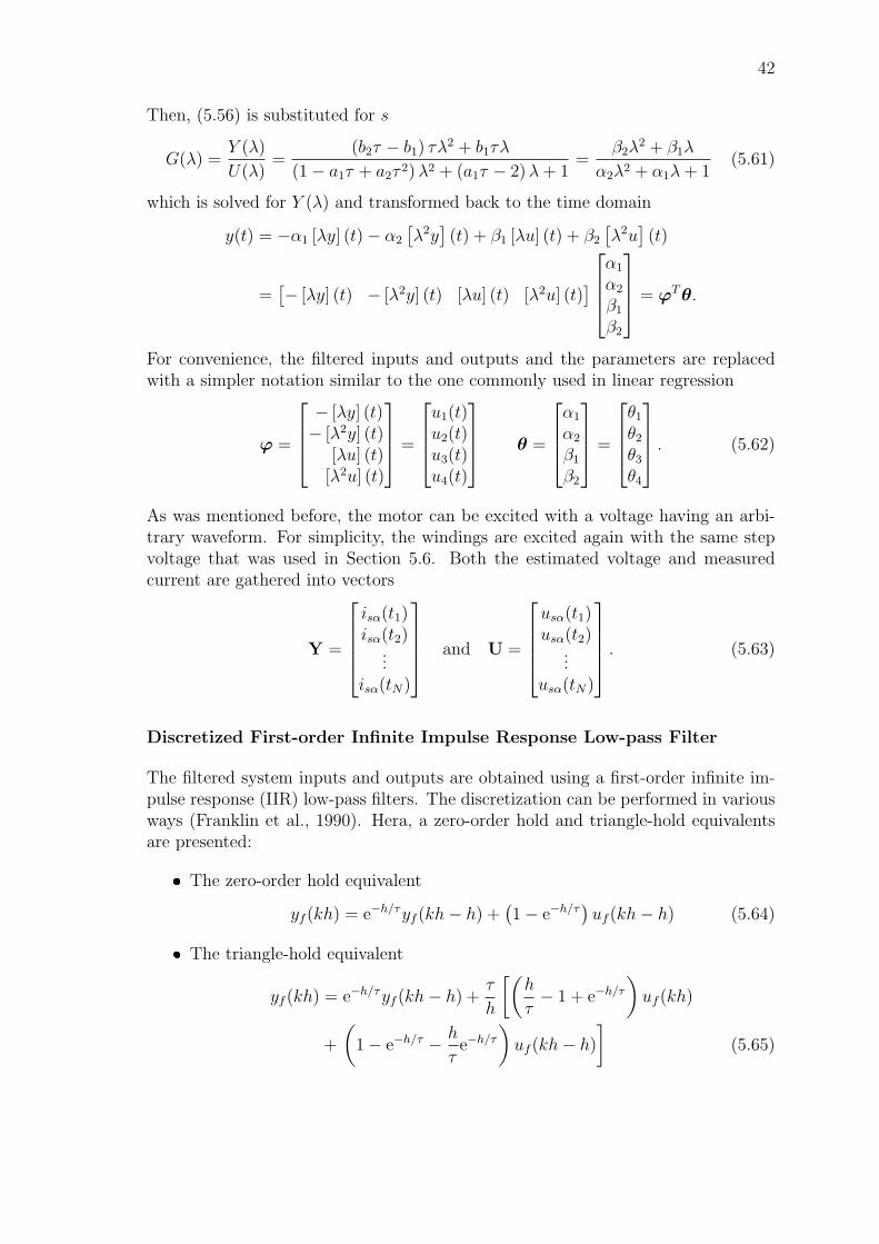
42

Then, (5.56) is substituted for s

G(λ) =Y (λ)

U(λ)=

(b2τ − b1) τλ2 + b1τλ

(1− a1τ + a2τ 2)λ2 + (a1τ − 2)λ+ 1=

β2λ2 + β1λ

α2λ2 + α1λ+ 1(5.61)

which is solved for Y (λ) and transformed back to the time domain

y(t) = −α1 [λy] (t)− α2

[λ2y]

(t) + β1 [λu] (t) + β2

[λ2u]

(t)

=[− [λy] (t) − [λ2y] (t) [λu] (t) [λ2u] (t)

] α1

α2

β1

β2

= ϕTθ.

For convenience, the filtered inputs and outputs and the parameters are replacedwith a simpler notation similar to the one commonly used in linear regression

ϕ =

− [λy] (t)− [λ2y] (t)

[λu] (t)[λ2u] (t)

=

u1(t)u2(t)u3(t)u4(t)

θ =

α1

α2

β1

β2

=

θ1

θ2

θ3

θ4

. (5.62)

As was mentioned before, the motor can be excited with a voltage having an arbi-trary waveform. For simplicity, the windings are excited again with the same stepvoltage that was used in Section 5.6. Both the estimated voltage and measuredcurrent are gathered into vectors

Y =

isα(t1)isα(t2)

...isα(tN)

and U =

usα(t1)usα(t2)

...usα(tN)

. (5.63)

Discretized First-order Infinite Impulse Response Low-pass Filter

The filtered system inputs and outputs are obtained using a first-order infinite im-pulse response (IIR) low-pass filters. The discretization can be performed in variousways (Franklin et al., 1990). Hera, a zero-order hold and triangle-hold equivalentsare presented:

The zero-order hold equivalent

yf (kh) = e−h/τyf (kh− h) +(1− e−h/τ

)uf (kh− h) (5.64)

The triangle-hold equivalent

yf (kh) = e−h/τyf (kh− h) +τ

h

[(h

τ− 1 + e−h/τ

)uf (kh)

+

(1− e−h/τ − h

τe−h/τ

)uf (kh− h)

](5.65)

43

where h is the inverse of the sampling frequency fs, which should be chosen higherthan the system bandwidth. However, too high a value causes numerical instabilities.

In practice, finite impulse response (FIR) filters may be preferred because such filtersare faster to execute in digital signal processors, and because IIR filters may causeoscillations when implemented with fixed-point arithmetics (Niiranen, 1999). Inaddition, FIR filters can be designed with completely linear phase response. Furtherinformation on digital filters can be found in (Smith, 2003).

Recursive Identification

The parameter vector θ is solved by means of recursive least-squares algorithm:

STEP 1. Choose the number of measurement points N , and the proper values forthe filter time constant τ , forgetting factor µ and the covariance matrix gain α, seeAppendix A.

STEP 2. Calculate the initial values for θ and P or initialize them as

θ(0) =

0000

, P(0) =

α 0 0 00 α 0 00 0 α 00 0 0 α

.STEP 3. Calculate the filtered inputs and outputs with, for example, (5.64).

STEP 4. Calculate the update coefficient

gi(N) =4∑j=1

pij(N)uj(N + 1), i = 1, 2, 3, 4,

γ(N) =

γ1(N)γ2(N)γ3(N)γ4(N)

=1

4∑i=1

ui(N + 1)gi(N) + µ

g1(N)g2(N)g3(N)g4(N)

.STEP 5. Calculate the parameter estimate

e(N + 1) = y(N + 1)−4∑i=1

θi(N)ui(N + 1),

θ(N + 1) =

θ1(N) + γ1(N)e(N + 1)θ2(N) + γ2(N)e(N + 1)θ3(N) + γ3(N)e(N + 1)θ4(N) + γ4(N)e(N + 1)

.

44

STEP 6. Calculate the estimate for the covariance matrix

pij(N + 1) =1

µ

(pij(N)− γi(N)

4∑l=1

plj(N)ul(N + 1)

), j = 1, 2, 3, 4,

P(N + 1) =

p11(N + 1) p12(N + 1) p13(N + 1) p14(N + 1)p21(N + 1) p22(N + 1) p23(N + 1) p24(N + 1)p31(N + 1) p32(N + 1) p33(N + 1) p34(N + 1)p41(N + 1) p42(N + 1) p43(N + 1) p44(N + 1)

.STEP 7. Stop if no more measurements, else go back to STEP 3.

Parameter Mappings

After the parameter vector (5.62) has been identified, the desired motor parametersare simply calculated from

Lσ =τ

β1

(5.66a)

Rs =1 + α1 + α2

β1 + β2

(5.66b)

LM =2 + α1 − β1Rs

β1 + β2

τ − Lσ (5.66c)

RR =β1 + β2

τ 2LM Lσ. (5.66d)

5.8 Frequency Response Identification

The time domain identification in the previous sections was based on feeding thestator windings with voltage or current pulses, which, by the definition of the Fouriertransform, contain infinitely many frequencies with decaying amplitudes whereas thestandstill frequency response (SSFR) identification methods are based on sinusoidalvoltages and currents with constant amplitudes and frequencies. Thus, the system isexcited with only one frequency at a time, and therefore it is easier to avoid excitingunwanted frequency dependent phenomenon.

The SSFR method has several advantages. For example, it is very accurate whenperformed with correlation method of frequency response (CMFR), which has alow computational burden and it gives good results even with poor signal-to-noiseratios. In addition, constant disturbances, like measurement offsets, are completelyeliminated from the results.

On the other hand, identification takes more time with the SSFR method as it isnecessary to wait for a certain period of time after changing the input frequencyfrom one to another so that the initial transients have decayed enough. Further-more, several periods have to be measured. Otherwise, the results are affected by

45

measurement noise. Recently, SSFR methods have successfully been applied to in-duction motors by Bunte and Grotstollen (1993), Sonnaillon et al. (2007) and Kwonet al. (2008).

The basis of the SSFR identification can be deduced from the way the motor currentsdivide between the stator and rotor circuits in steady-state conditions. When therotor is at standstill, the magnetizing and rotor currents are related to the statorcurrent by

IM =1√

1 + (ω1τr)2Is (5.67a)

IR =ω1τr√

1 + (ω1τr)2Is. (5.67b)

The magnitude of the magnetizing current IM approaches zero as the stator fre-quency approaches infinity. Therefore, the AC current will entirely flow in the rotor.On there hand, when the stator frequency approaches zero, the magnitude of therotor current IR approaches zero, which means that the AC current will entirely flowin the stator circuit. Thus, the stator and rotor parameters can be solved form thestator impedance (3.22) when both low and high frequencies are used.

The parameters, Lσ, LM and RR, should be identified from the effective statorinductance

Le(ω1) = Lσ +LM

1 + (ω1τr)2 (5.68)

as it is not affected by the stator resistance nor the nonlinear inverter resistanceRi(is), introduced in Section 5.2. There is a problem however. As the motor is notsupplied with a symmetrical sinusoidal three-phase supply, the input power is notconstant because the amplitudes of the current and voltage space vectors pulsatewith the stator frequency. As a consequence, the information of the phase anglevanishes every time a space vector becomes zero.

The inductance could be calculated recursively by solving a discretized version ofthe stator voltage equation

usα(t) = Reisα(t) + Ledisα(t)

dt(5.69)

as is done in (Bertoluzzo et al., 1997) and (Aiello et al., 2002). However, solving theresulting discrete autoregressive moving average has the same disadvantages thatwere discussed in the beginning of Section 5.7.

Fortunately, there is a better way. The effective stator inductance can be solvedfrom the reactive input power (3.25c)

Le(ω1) =usαisα· sin (ϕ1)

ω1

. (5.70)

46

if only the phase difference ϕ1 between the fundamental-frequency voltage and cur-rent phasors is known. This information is easily obtained using the correlationmethod of frequency response presented next.

Correlation Method of Frequency Response

The correlation method of frequency response (CMFR) is the basic tool in discreteFourier transform as it has an ability to find the amplitude ratio and phase differencebetween any two sinusoidal signals. The method is usually exploited in phase-lockedloops (PLL) and lock-in amplifiers (LIA) used in signal tracking applications. Forexample, the motor identification method presented in (Sonnaillon et al., 2007) usesthis technique, although different name is used.

A simple derivation of the method is presented below for a general sampled system,whose input and output signals, u(kh) and y(kh), are defined as

u(kh) = u sin (ω1kh) (5.71a)

y(kh) = y sin (ω1kh+ ϕ1)

= yc cos (ω1kh) + ys sin (ω1kh) . (5.71b)

whereas the amplitudes, y, yc and ys, are

y =√y2c + y2

s (5.72a)

yc = y sin (ϕ1) (5.72b)

ys = y cos (ϕ1) . (5.72c)

Now, the system gain K(ω1) and phase difference ϕ1(ω1) can be obtained from

K(ω1) =∣∣G(ejω1h)

∣∣ =y

u(5.73a)

ϕ1(ω1) = arctan

(ycys

)(5.73b)

if only the coefficients yc and ys are known.

Basically, the output signal is separated into components having 90-degree phaseshifts between each other by multiplying the output signal with a cosine and sinehaving the same frequency f1 as the input signal. Then, both components areintegrated over a measuring interval tm chosen as an integer multiple l of the periodt1 of the input frequency

tm = lt1 = l2π

ω1

, l ∈ 1, 2, . . . . (5.74)

During that time, N measurement points are taken from the output signal with asampling frequency fs = 1

h

N = tmfs + 1 =tmh

+ 1. (5.75)

47

h

t1

tm

Figure 5.8: Measured signal in the correlation method of frequency response.

Figure 5.8 illustrates the sampling process. In discrete time, the integrals are re-placed with the corresponding sums. As a consequence, the coefficients can becalculated from

yc =2

N

N−1∑k=0

y(kh) cos (ω1kh) (5.76a)

ys =2

N

N−1∑k=0

y(kh) sin (ω1kh) . (5.76b)

More thorough derivation of the method can be found in (Franklin et al., 1990, p.354).

SSFR Identification Process

The stator windings are fed with a combination of DC and AC currents

isα(t) = Idc +√

2Iac sin (ω1t) . (5.77)

The purpose of the DC component Idc is to magnetize the motor in a desired oper-ation point, and to minimize the nonlinear change in magnetization caused by themagnetic hysteresis and saturation otherwise present when the motor is magnetizedwith a sinusoidal current alone. Furthermore, the added DC component can be usedto excite the motor above the nonlinear inverter region if it is a problem, see Figure5.2.

In the following, the DC component is chosen as the nominal magnetizing currentand the angular frequency of the sine wave as the nominal ω1N . Now, the total

48

leakage inductance can be solved from the effective stator inductance (5.70) as theyare approximately equal in this operation point

Lσ ≈ Le(ω1N). (5.78)

To identify the transformed magnetizing inductance LM and rotor resistance RR, themotor has to be fed again with the above combination of DC and AC currents, butthis time the effective stator inductance must be measured with at least two differentstator frequencies. These two frequencies are chosen from the low-frequency end,close to the nominal angular slip frequency ω2N .

An estimate for the proper stator current that will cause the nominal magnetizingcurrent at low frequencies can be obtained from the displacement power factor

IMN ≈ IN sinϕN = IN

√1− (cosϕN)2 (5.79a)

IRN ≈ IN cosϕN (5.79b)

where IMN and IRN are the magnetizing and rotor currents with nominal statorcurrent, respectively. Then, the correct stator current is obtained from Equation(5.67a)

Is(ω1) =

√1 + (ω1τr)

2IMN (5.80)

where the rotor time constant is estimated from the motor name-plate (5.14).

After the measurements have been taken, the transformed magnetizing inductancecan be solved from a linear 2× 2 system

1

Le(ωa)− LσLM − ω2

aτ2r = 1 (5.81a)

1

Le(ωb)− LσLM − ω2

b τ2r = 1 (5.81b)

where ωa and ωb are the different angular measurement frequencies. The transformedrotor resistance is then easily solved from the estimate of the rotor time constant

RR =LMτr. (5.82)

5.9 Magnetizing Curve Identification

If the motor is going to be operated above the rated speed nN with reduced rotorflux linkage, or if more torque is wanted with less current, or if the magnetic circuitis too nonlinear, a constant value for the magnetizing inductance is inadequate forgood control performance. In such conditions, the saturation curve has to be knownfor the rotor flux linkage or the magnetizing inductance. Such curves are depicted in

49

Figures 5.9 and 5.10. Unfortunately, the task of finding these curves is the hardestpart in standstill identification as several tests have to be performed, and as theprocess is complicated at low voltages by the inverter nonlinearity and magnetichysteresis, particularly when step response tests are used. Therefore, only a shortintroduction to one method is presented below as a thorough discussion of the topicis beyond the scope of this Master’s thesis.

The magnetizing inductance is divided into static and dynamic parts where theformer is defined as the slope of the straight line drawn from the origin to a particularoperating point in the curve of the rotor flux linkage versus the magnetizing current

LM(iM) =

∣∣∣ψR

(iM)∣∣∣

|iM |(5.83)

whereas the latter is the slope of the tangent at that point

LD(iM) =d∣∣∣ψ

R(iM)

∣∣∣d |iM |

(5.84a)

= LM(iM) +dLM(iM)

d |iM ||iM | . (5.84b)

The problem is to find a smooth function that accurately estimates the static magne-tizing inductance. For example, Ruff and Grotstollen (1996) have used an exponentfunction

LM(iM) = La eKa |iM | + Lb eKb |iM | + Lc (5.85)

where the parameters La and Lc are positive, and Lb, Ka and Kb negative. As theabove equation is nonlinear with respect to the parameters, it cannot be solved withlinear regression, which means that a very time-consuming numerical optimizationshould be used. Therefore, other simpler functions are preferred in literature.

Yet, single values for the static magnetizing inductance can still be solved rathereasily by combining the flux linkage equations (3.16), the stator voltage equation(3.17a) and the nonlinear inverter resistance (5.20b). It follows that the rotor fluxlinkage can be obtained from

ψRα(t) = ψRα(0) +

t∫0

[usα,ref (t

′)− Rei

(isα(t′)

)isα(t′)

]dt′ − Lσisα(t) (5.86)

where the initial value ψRα(0) exists due to the magnetic hysteresis. Equation (3.16c)yields an expression for the magnetizing inductance

LM(isα,i) =ψRα,i(t)

iMα,i(t)

∣∣∣∣t→∞

=ψRα,i(t)

isα,i(t)

∣∣∣∣t→∞

i ∈ 0, 1, 2, . . . (5.87)

where the last equality holds if the motor is fed with constant DC voltages, in whichcase the steady-state stator current equals the steady-state magnetizing current.

50

ψR=LM (iM )iM

ψRD=LD (iM )iM

Figure 5.9: Rotor flux linkage as a function of the magnetizing current.

Figure 5.10: Static magnetizing inductance as a function of the magnetizing current.

After those single values are solved for the magnetizing inductance, the real magne-tizing curve can be approximated using linear interpolation between two consecutivevalues.

More detailed information about the used method can be found in (Ruff and Grot-stollen, 1996) and (Sukhapap and Sangwongwanich, 2002), and a comparison ofdifferent types of functions that have been used for estimating the static magnetiz-ing inductance in (Ganji et al., 1996). Methods based on SSFR can be found in(Bunte and Grotstollen, 1993), (Sonnaillon et al., 2007).

51

6 Simulation Results

An ideal induction motor without any nonlinearities was identified with both thestep and frequency response methods using simulated input-output data. The sim-ulations were performed with MATLAB Simulink, which is a numerical computingenvironment produced by Mathworks. The motor parameters are Lσ = 7.3 mH,Rs = 0.5 Ω and LM = 65.0 mH and RR = 0.7 Ω, which yield the following timeconstants: τ ′s = 6.1 ms, τs = 144.6 ms and τr = 92.9 ms. That is, the two poles ofthe motor’s standstill transfer function (5.38) are located at 0.7 Hz and 27.2 Hz.

Step Response Test with SVF

In the first simulation, the motor was fed with a voltage pulse shown in Figure 6.1using ’Case 1’-excitation, see Section 5.4. The pulse-duration was one second and ithad an amplitude of 10 volts. The simulated voltage and current vectors were thenprocessed by the state variable filtering method using the recursive identificationalgorithm presented in Section 5.7.

The algorithm was run several times with different values for the low-pass filtercut-off frequency f0 and sampling frequency fs. Then, a second test was performedsimilarly with an exception that bandwidth-limited white noise with 100 mA meanand 100 mA standard deviation was added to the stator current to model measure-ment noise and offset, see Figure 6.2. Results from both tests are presented in Table6.1.

It is observed that the stator resistance is the only parameter that stays rather ac-curate regardless of the chosen filter cut-off frequency or the sampling frequency.Furthermore, it appears that the sampling frequency has least effect when the fil-ter cut-off frequency is selected close to the lower pole. Moreover, it seems thatover-sampling tends to increase inductances, which is probably caused by increasingnumerical problems in the least-squares method, i.e. the input-output data does nothave enough variations. All in all, the chosen level of measurement noise and offsethas a very small effect on the estimated parameters. In general, the estimates arenot that much affected by the white noise no matter how high compared to highlevels of measurement offset.

There is also a fundamental problem in induction motor identification caused bythe fact that the two poles are so far from each other in the frequency domain,which means that the lower pole, approximately corresponding to the LM and RR,should be identified with a lower filter cut-off frequency, and the higher pole, roughlycorresponding to the Lσ, with a higher cut-off frequency. Thus, in this case, thevalues estimated with f0 and fs near 30 Hz and 5 kHz, respectively, are likely to bemore correct for the Lσ than for the others, and vice versa when f0 is near 1 Hz.

52

Figure 6.1: Stator current response to a step voltage excitation. fs = 500 Hz.

Figure 6.2: Stator current response to a step voltage excitation when measurementnoise and offset are modeled. fs = 500 Hz.

53

Table 6.1: Results from the first (-) and second (noise) step response test. f0 is thefilter cut-off frequency and fs the sampling frequency.

[Hz] [kHz] Lσ [mH] Rs [Ω] LM [mH] RR [Ω]f0 fs - noise - noise - noise - noise

1.0 10.0 8.1 9.1 0.50 0.50 72.2 72.0 0.70 0.665.0 10.0 8.1 8.1 0.50 0.50 72.1 72.6 0.70 0.6930.0 10.0 8.1 7.9 0.50 0.50 71.5 71.2 0.70 0.7150.0 10.0 8.0 7.8 0.50 0.50 71.0 70.7 0.70 0.72100.0 10.0 7.9 7.3 0.50 0.50 69.9 62.6 0.71 0.88500.0 10.0 7.1 2.4 0.50 0.53 62.1 42.0 0.76 9.231.0 5.0 7.7 9.0 0.50 0.50 68.3 68.0 0.70 0.655.0 5.0 7.7 7.7 0.50 0.50 68.2 68.7 0.70 0.6930.0 5.0 7.6 7.5 0.50 0.50 67.1 67.4 0.71 0.7150.0 5.0 7.5 7.3 0.50 0.50 66.2 65.4 0.71 0.73100.0 5.0 7.3 6.5 0.50 0.51 64.2 55.2 0.72 0.98500.0 5.0 6.2 2.4 0.51 0.53 51.3 33.8 0.84 9.771.0 1.0 7.6 9.0 0.50 0.50 65.2 64.7 0.70 0.645.0 1.0 7.4 7.4 0.50 0.50 64.5 65.1 0.70 0.6830.0 1.0 6.9 6.8 0.50 0.50 59.8 59.7 0.73 0.7450.0 1.0 6.7 6.3 0.50 0.50 56.4 53.9 0.76 0.83100.0 1.0 6.2 4.9 0.51 0.52 49.1 39.1 0.85 1.40500.0 1.0 3.9 2.3 0.53 0.53 16.6 12.5 1.91 7.631.0 0.5 8.1 9.8 0.50 0.50 64.3 63.6 0.69 0.625.0 0.5 7.8 7.8 0.50 0.50 62.9 63.4 0.69 0.6830.0 0.5 6.9 6.7 0.50 0.50 54.2 53.8 0.73 0.7550.0 0.5 6.5 5.9 0.50 0.50 48.6 45.5 0.76 0.86100.0 0.5 5.5 4.5 0.51 0.52 37.3 29.4 0.87 1.41500.0 0.5 1.8 1.4 0.52 0.53 9.5 6.8 1.22 3.30

Real 7.3 0.5 65.0 0.7

54

Frequency Response Test with CMFR

As a first SSFR test, it was studied how accurately the CMFR method finds thetotal stator leakage inductance with and without measurement offset and noise whenthe ratio of the sampling frequency and the stator frequency was varied from 2.5 to80. The measurement noise was modeled again as a bandwidth-limited white noisebut this time a low signal-to-noise ratio, 5.1 dB, was used: standard deviation 2.23A and mean 1.0 A. Furthermore, the measurement duration tm was varied from oneto three periods of f1 to see how the averaging improves accuracy. Test results arepresented in Table 6.2 and the input-output signals in Figure 6.3.

As was expected, the method found the correct value for the total stator leakage in-ductance very accurately even in the presence of heavy measurement noise and hugeoffset that would have ruined the estimate if the step response method were used.In fact, due to the method’s characteristics, it is completely immune to measure-ment offsets. It was also rather surprising how well the CMFR method performedwhen only one period of test signals was measured in the noise-free case. Further-more, the parameter accuracy was higher than expected even with very low samplingfrequencies.

As a second SSFR test, the motor was fed again with the ’Case 1’-excitation butthis time three different test frequencies were used at a time: 50.0, 1.0 and 0.5Hz. Moreover, the offset and noise were both reduced to a more reasonable value:100 mA. The simulated voltage and current vectors were sampled with a frequencytwenty times higher than that of the excitation, after which one period of test signalswas removed from the beginning of both vectors to be sure that the initial transientswere decayed enough. Then, both vectors were processed with the CMFR methodwhose measurement time was varied as in the first test. Results are presented inTable 6.3, and the signal waveform is plotted in the middle of Figure 6.3.

It is observed that the accuracy of the identified parameters is similar to thoseobtained from the step response test as the identified system was linear. In addition,the frequency response test took three to six times longer to complete than thestep response test. However, the SSFR method has superior accuracy even withpoor signal-to-noise ratios, and the identified parameters are less affected by thenonlinearities.

55

Figure 6.3: Current response to sinusoidal voltage excitation with and without mea-surement noise. Sampling frequency is 20f1 in the plots at the top and middle, and80f1 in the one at the bottom.

56

Table 6.2: The effect of the chosen sampling frequency and test duration in theCMFR method. Initial transients are removed. Test frequency is 50.0 Hz. Mea-surement noise and offset are modeled as bandwidth-limited white noise with 1.0 Amean and 2.23 A standard deviation. Signal-to-noise ratio is approximately 5.1 dB.

Lσ [mH]- Offset + Noise

fs/f1 t1 2t1 3t1 t1 2t1 3t180 7.4 7.4 7.4 8.5 7.4 7.840 7.5 7.4 7.4 6.9 6.7 7.320 7.7 7.5 7.5 11.8 6.4 7.810 8.1 7.8 7.6 9.0 8.3 7.35 7.9 7.5 7.5 8.5 5.5 4.1

2.5 7.5 4.2 7.6 6.7 3.4 6.52 0.0 0.0 0.0 0.0 0.0 0.0

Real 7.3

Table 6.3: Results from the simulated standstill frequency response test. The effec-tive stator inductance is measured at 50.0, 1.0 and 0.5 Hz. The level of noise andoffset are reduced to 100 mA. tm is the time used measuring one frequency. Σtm isthe total test duration. Sampling frequency is fs = 20f1.

tm Σtm [s] Lσ [mH] LM [mH] RR [Ω]t1 6.04 7.9 63.5 0.712t1 9.06 7.5 64.5 0.703t1 12.08 7.5 64.7 0.69

Real 7.3 65.0 0.7

57

7 Experimental Results

The studied identification methods were also investigated with experimental tests.A typical elevator motor was identified using the equipment listed in Table 7.1. Themotor name-plate is given in Table 7.2.

The first parameter estimates were calculated from the name-plate, after which themotor was identified with a basic locked rotor and no-load tests (LRNL). Subse-quently, the identification was performed with the step response method (SR), thestate variable filtering method (SVF) and the frequency response method (FR) in-troduced in Sections 5.6, 5.7 and 5.8, respectively. The CMFR method was not usedbut the system gain and phase were measured with an oscilloscope.

In the SR and SVF tests, the motor was supplied with a DC power source, andthe stator voltages were measured with differential high-voltage probes whereas thecurrents were measured with shunts. The measurements were recorded with a three-phase power analyzer, and processed in MATLAB. Figure 7.1 shows what happensto the current response when the magnetic circuit saturates, i.e. the slope of thecurrent increases. Table 7.3 presents the results from the SVF test. Due to themagnetic hysteresis, the falling edge of the current response was not used in thecalculations as it would have caused erroneous results.

In the LRNL and FR tests, the motor was supplied with a frequency converter.This time, the stator voltage and current measurements were fed through an analog8th-order low-pass filter with a Butterworth response to extract the fundamental-frequency component from the pulse-width modulated stator voltage, and to keepboth measurements equally delayed. Furthermore, in the FR test, the effect ofhysteresis was minimized using constant magnetization with a DC component aswas explained in Section 5.8.

From the results of Table 7.4, it is observed how the studied methods gave re-sults that are rather close to each other, although the approaches were completelydifferent. However, it might be just a lucky coincidence that the name-plate approx-imation was so accurate for this particular motor. The table also reveals how theparameters obtained from the step response methods are affected by the rotor-barskin effect as the rotor resistances are almost two times higher than those from theLRNL and FR tests. However, the SVF based SR method managed to identifythe transformed magnetizing inductance with almost the same accuracy as the FRmethod. Furthermore, the tests with only few measurements, like the SR test inthis case, are very sensitive to measurement errors.

58

Table 7.1: Test equipment.

• KONE proprietary frequency converter• Delta Elektronika Power Supply SM 70-90• LEM Norma 5000 Power Analyzer• Tektronix TDS3014 Oscilloscope• Kemo VBF 8 Dual Variable Filter

Table 7.2: The name-plate of the tested induction motor Elemol CTF 160M.30R.

Power 7.5 kWRated voltage 340 VRated current 23 APower factor 0.8Frequency 50 HzRated speed 950 rpmRotor inertia 0.19 kgm2

Table 7.3: Results from the experimental step response test.

f0 [Hz] fs [kHz] Lσ [mH] Rs [Ω] LM [mH] RR [Ω]1.0 5.0 9.4 0.48 65.1 0.875.0 5.0 8.0 0.48 66.8 0.8930.0 5.0 7.3 0.48 65.5 0.941.0 1.0 9.4 0.48 65.1 0.875.0 1.0 8.0 0.48 66.1 0.8930.0 1.0 7.1 0.48 61.1 0.971.0 0.5 9.7 0.48 64.6 0.855.0 0.5 8.1 0.48 64.9 0.8730.0 0.5 7.1 0.48 56.4 1.00

Table 7.4: Experimental results from different identification tests.

Test method Motor parameters Notes

Lσ [mH] Rs [Ω] LM [mH] RR [Ω]

Name-plate 6 0.7 62 0.7 Rs ≈ RR, Lσ ≈ 0.1LMLRNL 6 0.48 67 0.7 50 Hz, 2.5 HzSR test 11 0.48 54 1.2 2 pointsSVF 7.3 0.48 66 0.9 f0 = 1.0, 30.0 Hz, 5.5 V / 11.7 AFR test 7.5 - 63 0.5 50, 2.5, 0.5 Hz

59

Figure 7.1: ’Unsaturated’ (top) and saturated (middle) current responses to a stepvoltage excitation produced with a DC power supply. The figure bottom shows thedata used in the SVF method to avoid hysteresis and saturation.

60

8 Conclusions

The object of this master’s thesis was to find a method that could accurately identifythe electrical parameters of the mathematical model of the induction motor that ispowered with a frequency converter in a condition where the motor is not allowedto rotate. The identification was found possible if the motor is excited with sucha three-phase voltage that does not produce torque. The desired parameters canthen be solved from the resulting voltages and currents with system identificationmethods based on transient and frequency responses, respectively.

The identification process is complicated because neither the output voltage of thepulse-width modulated inverter nor the rotor currents of the induction motor witha squirrel-cage rotor can be measured. Thus, both variables have to be estimatedfrom the commanded stator voltage and the measured stator current. However,the relationship between the two is nonlinear if the voltage drops caused by thetransistors and the freewheeling diodes, and the reduced pulse-width caused by thedead-time are not compensated. Thus, if not taken into account, the aforementionednonlinearity will act as an additional series resistance that cannot be separated fromthe motor’s stator resistance without impractical phase voltage sensors.

In the studied transient response method, the stator windings were fed with a stepvoltage, whose magnitude was selected such that the resulting current did not causemagnetic saturation. The measured current and the estimated voltage were pro-cessed with a method called state variable filtering (SVF) that was applied to in-duction motor at standstill, and the produced linear system of equations was solvedwith recursive least-squares algorithm. The desired motor parameters were thencalculated from the obtained parameter vector.

On the other hand, the studied frequency response method was based on the com-bination of DC and AC excitations. The DC component was used to set the desiredlevel of magnetization while the AC component and the corresponding voltage wereprocessed using the correlation method of frequency response. As a result, thesystem gain and phase difference were obtained at selected frequencies. This in-formation was then used in calculating the input inductance, from which the othermotor parameters were solved.

It was observed that the methods based on transient response were faster to conductthan those based on frequency response as the latter methods require several sec-onds, even minutes, to complete. However, the former methods produce incorrectresults when applied to systems whose parameters change with frequency as thenon-sinusoidal excitations used in such methods contain several frequencies. There-fore, methods with such excitations should not be used when identifying inductionmotors where the rotor resistance and leakage inductance change with frequency dueto the skin and proximity effects, or else the results have to be corrected for sucheffects. According to author’s opinion, frequency response methods should be usedas then the obtained parameter accuracy is only restricted by the quality of the volt-age estimation and current measurements. Moreover, more code has to be writtenif transient response methods are going to be implemented as such methods usually

61

require curve-fitting algorithms, e.g. recursive least-squares or maximum likelihoodones.

Although the transient response methods are not recommended when identifyingthe electrical parameters, they could be used to identify systems without frequencydependencies. For example, the SVF method could be modified to track variationsin the mechanical parameters.

Furthermore, if the motor is going to be operated above the rated speed with reducedrotor flux linkage, or if more torque is wanted with less current, the magnetizationcurve should also be identified. The best method for this purpose is the frequency re-sponse one as then the parameter accuracy is not affected by that of stator resistanceas it is the case with transient response methods.

If further investigations were conducted, it should be studied how the parametervariations could be tracked when the motor heats up. For example, model-referenceadaptive system based estimators or the SVF method could be used for this purpose.

62

References

Aiello, M., Cataliotti, A., and Nuccio, S. (2002). “A fully-automated procedure formeasuring the electrical parameters of an induction motor drive with rotor atstandstill.” In 19th IEEE Instrumentation and Measurement Technology Confer-ence, vol. 1, pp. 681–685.

Ambrozic, V., Cajhen, R., and Nastran, J. (1993). “A step voltage method fordetermination of an induction motor rotor time constant in cold state.” IEEEInternational Symposium on Industrial Electronics in Budapest, pp. 85–89.

Ba-Razzouk, A., Cheriti, A., and Sicard, P. (2002). “Implementation of a DSP basedreal-time estimator of induction motors rotor time constant.” IEEE Transactionson Power Electronics, 17(4), pp. 534–542.

Barrero, F., Perez, J., Millan, R., and Franquelo, L. (1999). “Self-commissioning forvoltage-referenced voltage-fed vector controlled induction motor drives.” In The25th Annual Conference of the IEEE Industrial Electronics Society, vol. 3, pp.1033–1038.

Bertoluzzo, M., Buja, G. S., and Menis, R. (1997). “Inverter voltage drop-free recur-sive least-squares parameter identification of a PWM induction motor at stand-still.” In Proceedings of the IEEE International Symposium on Industrial Elec-tronics 1997, vol. 2, pp. 649–654.

Bertoluzzo, M., Buja, G. S., and Menis, R. (2001). “Self-commissioning of RFO IMdrives: One-test identification of the magnetization characteristic of the motor.”IEEE Transactions on Industry Applications, 37(6), pp. 1801–1806.

Blaabjerg, F. and Pedersen, J. K. (1994). “An ideal PWM-VSI inverter using onlyone current sensor in the DC-link.” In Proceedings of the 5th International Con-ference on Power Electronics and Variable-Speed Drives, pp. 458–464.

Bunte, A. and Grotstollen, H. (1993). “Parameter identification of an inverter-fed in-duction motor at standstill with a correlation method.”Fifth European Conferenceon Power Electronics and Applications, 5, pp. 97–102.

Buja, G. S., Menis, R., and Valla, M. I. (1995).“MRAS identification of the inductionmotor parameters in PWM inverter drives at standstill.”In Proceedings of the 1995IEEE IECON 21st International Conference on Industrial Electronics, Controland Instrumentation, vol. 2, pp. 1041–1047.

Choi, J.-W. and Soul, S.-K. (1994). “New dead time compensation eliminating zerocurrent clamping in voltage-fed PWM inverter.” In Conference Record of the 1994IEEE Industry Applications Society Annual Meeting, no. 2-6, pp. 977–984.

Cirrincione, M., Pucci, M., and Vitale, G. (2002). “A least-squares based method-ology for estimating the electrical parameters of induction machine at standstill.”In IEEE International Symposium on Industrical Electronics, vol. 2, pp. 541–547.

63

Couto, E. B. and de Aguiar, M. L. (1998). “Parameter identification of inductionmotors using DC step excitation at standstill.” In IEEE International Symposiumon Industrial Electronics, vol. 2, pp. 468–471.

Dell’Aquila, A., Giliberti, V., Lovecchio, F., and Salvatore, L. (1994). “Real-timeestimation of induction motor parameters by lse.”In 20th International Conferenceon Industrial Electronics, Control and Instrumentation, vol. 3, pp. 2127–2131.

do Prado Junior, A., Heerdt, J. A., and Junior, S. I. S. (2002).“Off-line identificationof PWM driver induction motors using reference voltages.” In IEEE 2002 28thAnnual Conference of the Industrial Electronics Society, vol. 3, pp. 2057–2062.

Franklin, G. F., Powell, J. D., and Workman, M. L. (1990). Digital Control ofDynamic Systems. Addison-Wesley, CA.

Ganji, A. A., Guillaume, P., Pintelon, R., and Lataire, P. (1996). “Identification ofthe induction motor dynamic and static inductance with regard to saturation.” InPower Electronics and Variable Speed Drives, no. 429, pp. 42–47.

Garnier, H., Mensler, M., and Richard, A. (2003). “Continuous-time model identi-fication from sampled data: implementation issues and performance evaluation.”International Journal of Control, 76(13), pp. 1337–1357.

Garnier, H. and Young, P. (2004). “Time-domain approaches to continuous-timemodel identification of dynamical systems from sampled data.” In American Con-trol Conference, vol. 1, pp. 667–672.

Hanselman, D. and Peake, W. (1995). “Eddy-current effects in slot-bound conduc-tors.” In IEE Proceedings Electric Power Applications, vol. 142, pp. 131–136.

Harnefors, L. (2003). Control of Variable-Speed Drives. Applied Signal Processingand Control, Department of Electronics, University of Malardalen, Vasteras, Swe-den.

Hagglund, T. and Astrom, K. J. (2006). Advanced PID Control. The Instrumenta-tion, Systems, and Automation Society, Research Triangle Park, NC.

Holtz, J. (1994). “Pulsewidth modulation for electronic power conversion.” In Pro-ceedings of the IEEE, vol. 82, pp. 1194–1214.

Holtz, J. (1995). “The representation of AC machine dynamics by complex signalflow graphs.” IEEE Transactions on Industrial Electronics, 42(3), pp. 263–271.

IEC (1994). IEC Standard 60034-1: Rotating Electrical Machines - Part 1: Ratingand Performance. International Electrotechnical Commission.

IEEE (1991). IEEE Standard Test Procedure for Polyphase Induction Motors andGenerators. No. Std 112-1991, The Institute of Electrical and Electronics Engi-neers, Inc.

64

Johansson, R. (1986). “Identification of continuous-time dynamic systems.” In IEEE25th Conference on Decision and Control, pp. 1653–1658.

Johansson, R. (1993). System Modeling and Identification. Prentice Hall, NJ.

Kerkman, R. J. (1985). “Steady-state and transient analyses of an induction ma-chine with saturation of the magnetizing branch.” IEEE Transactions on IndustryApplications, 21(1), pp. 226–234.

Klaes, N. R. (1993).“Parameter identification of an induction machine with regard todependencies on saturation.” IEEE Transactions on Industry Applications, 29(6),pp. 1135–1140.

Kreyszig, E. (1999). Advanced Engineering Mathematics, 8th ed. John Wiley, Hobo-ken, NJ.

Krishnan, R. (2001). Electric Motor Drives: Modeling, Analysis and Control. Pren-tice Hall, Upper Saddle River.

Krishnan, R. and Bharadwaj, A. S. (1991). “A review of parameter sensitivity andadaptation in indirect vector controlled induction motor drive systems.” IEEETransactions on Power Electronics, 6(4), pp. 695–703.

Kwon, W. H., Lee, C. H., Youn, K. S., and Cho, G. H. (1994). “Measurement ofrotor time constant taking into account magnetizing flux in the induction motor.”In Conference Record of the 1994 IEEE Industry Applications Society AnnualMeeting, vol. 1, pp. 88–92, IEE.

Kwon, Y.-S., Lee, J.-H., Moon, S.-H., Kwon, B.-K., Choi, C.-H., and Seok, J.-K.(2008). “Standstill parameter identification of vector-controlled induction motorsusing frequency characteristics of rotor bars.” IEEE Industry Applications SocietyAnnual Meeting, pp. 1–7.

Leggate, D. and Kerkman, R. J. (1997). “Pulse-based dead-time compensator forPWM voltage inverters.” IEEE Transactions on Industrial Electronics, 44(2), pp.191–197.

Levi, E., Sokola, M., Boglietti, A., and Pastorelli, M. (1996). “Iron loss in rotor-flux-oriented induction machines: identification, assessment of detuning, and compen-sation.” IEEE Transactions on Power Electronics, 11(5).

Ljung, L. (1987). System identification: theory for the user. Prentice Hall, NJ,United States.

Ljung, L. and Soderstrom, T. (1983). Theory and Practice of Recursive Identifica-tion. MIT Press, MA, United States.

Martin, F. (1996). Semikron Power Electronics Catalogue. Semikron International,Nurnberg, Germany.

65

Melkebeek, J. A. A. and Novotny, D. W. (1983). “The influence of saturation oninduction machine drive dynamics.” IEEE Transactions on Industry Applications,19(5), pp. 671–681.

Meyer, C. D. (2000). Matrix Analysis and Applied Linear Algebra. Society for In-dustrial and Applied Mathematics, Philadelphia, PA.

Michalik, W. (1998). “Standstill estimation of electrical parameters in motors withoptimal input signals.” In Second IEEE International Caracas Conference on De-vices, Circuits and Systems, pp. 407–413.

Minami, K., Velez-Reyes, M., Elten, D., Verghese, G. C., and Filbert, D. (1991).“Multi-stage speed and parameter estimation for induction machines.” In 22ndAnnual IEEE Power Electronics Specialists Conference Record, no. 24-27, pp.596–604.

Mohan, N., Undeland, T. M., and Robbins, W. P. (2003). Power Electronics: Con-verters, Applications and Design, 3rd ed. John Wiley, Hoboken, NJ.

Moon, S. and Keyhani, A. (1993). “Estimation of induction machine parametersfrom standstill time domain data.” Conference Record of the 1993 IEEE IndustryApplication Society Annual Meeting, 1(3-8), pp. 336–342.

Munoz, A. R. and Lipo, T. A. (1999). “On-line dead-time compensation techniquefor open-loop PWM-VSI drives.” IEEE Transactions on Power Electronics, 14(4),pp. 683–689.

Niiranen, J. (1999). Sahkomoottorikayton digitaalinen ohjaus (Digital Control ofElectric Motor Drives), 2nd ed. Otatieto, Helsinki, Finland.

Rasmussen, H., Knudsen, M., and Tønnes, M. (1996). “Parameter estimation ofinverter and motor model at standstill using measured currents only.” In Proceed-ings of the IEEE International Symposium on Industrial Electronics, vol. 1, pp.331–336.

Rowan, T., Kerkman, R., and Leggate, D. (1989). “A simple on-line adaptation forindirect field orientation of an induction machine.” In Conference Record of the1989 IEEE Industry Applications Society Annual Meeting, vol. 1, pp. 579–587.

Ruff, M. and Grotstollen, H. (1996). “Off-line identification of the electrical param-eters of an industrial servo drive system.” Conference Record of the 1996 IEEEIndustry Applications, 1(6-10), pp. 213–220.

Sadarangani, C. (2000). Electrical Machines - Design and Analysis of Induction andPermanent Magnet Motors. US-AB, Stockholm, Sweden.

Salomaki, J. (2003). Suppression of mechanical vibrations in speed controlled elevatordrives. Master’s thesis, Helsinki University of Technology, Finland.

66

Seok, J.-K., Moon, S.-I., and Sul, S.-K. (1997). “Induction machine parameter iden-tification using PWM inverter at standstill.” IEEE Transactions on Energy Con-version, 12(2), pp. 127–132.

Shaw, S. R. and Leeb, S. B. (1999). “Identification of induction motor parametersfrom transient stator current measurements.” IEEE Transactions on IndustrialElectronics, 46(1), pp. 139–149.

Slemon, G. R. (1989). “Modelling of induction machines for electric drives.” IEEETransactions on Industry Applications, 25(6), pp. 1126–1131.

Smith, S. W. (2003). Digital Signal Processing: A Practical Guide for Engineers andScientists. Newnes, Burlington, MA.

Sonnaillon, M., Bisheimer, G., Angelo, C. D., and Garcia, G. (2007). “Automaticinduction machine parameters measurement using standstill frequency-domaintests.” IET Electronic Power Applications, 1(5), pp. 833–838.

Stolt, L. (2005). Speed Sensorless Control of Squirrel Cage Induction Motors inElevator Applications. Master’s thesis, Helsinki University of Technology, Finland.

Sukhapap, C. and Sangwongwanich, S. (2002). “Auto tuning of parameters andmagnetization curve of an induction motor at standstill.” In IEEE InternationalConference on Industrial Technology, vol. 1, pp. 101–106.

Toliyat, H. A., Levi, E., and Raina, M. (2003). “A review of RFO induction mo-tor parameter estimation techniques.” IEEE Transactions on Energy Conversion,18(2), pp. 271–283.

Urasaki, N., Senjyu, T., Uezato, K., and Funabashi, T. (2005). “An adaptive dead-time compensation strategy for voltage source inverter fed motor drives.” IEEETransactions on Power Electronics, 20(5), pp. 1150–1160.

Vas, P. (1993). Parameter Estimation, Condition Monitoring, and Diagnosis of Elec-trical Machines. Clarendon Press, Oxford.

Wang, C., Novotny, D. W., and Lipo, T. A. (1988). “An automated rotor time con-stant measurement system for indirect field-oriented drives.” IEEE Transactionson Industry Applications, 24(1), pp. 151–159.

White, T. and Hinton, J. (1995). “Compensation for the skin effect in vector-controlled induction motor drive systems.” In Electrical Machines and Drives,1995. Seventh International Conference on (Conf. Publ. No. 412), pp. 301–305.

Ylen, J.-P. (2008). Luentomonisteet tietokonemallintamisesta (Lecture notes inComputer modeling). Helsinki University of Technology.

67

Appendix A: Linear Regression

A system, whose output equation is, for example, an nth order polynomial,

y(t) = θ0 + θ1u(t) + . . .+ θnun(t) (A1)

can be written in a matrix form

y(t) =[1 u(t) . . . un(t)

]θ0

θ1...θn

= ϕTθ. (A2)

The model parameters θi can be solved with linear regression. First, a data setof N measurement points is gathered from the system input u(t = kh) and outputy(t = kh) with a sampling period h. Then, the measurements are put into an outputvector Y and a regressor matrix Φ

Y =

y(k1)y(k2)

...y(N)

, Φ =

ϕT (k1)ϕT (k2)

...ϕT (N)

=

1 u(k1) . . . un(k1)1 u(k2) . . . un(k2)...

.... . .

...1 u(N) . . . un(N)

. (A3)

The measurements describe the original system with a matrix equation

Y = Φθ + e (A4)

where the vector eT =[e(k1) e(k2) · · · e(N)

]contains errors between the mea-

surements and the model.

The object is to find a parameter vector θ describing the real system output asclosely as possible. This vector can be found by minimizing the square of errors

J(θ) =1

2

N∑i=1

e2i =

1

2eTe, e = Y − Y = Y −Φθ (A5)

which can be done with the least-squares (LS) estimate

θ =(ΦTΦ

)−1ΦTY = Φ†ΦTY. (A6)

As this involves calculating a time-consuming pseudo-inverse Φ† of an N×N matrix,which might have bad numerical properties, it is better to use a recursive version ofthe least-squares (RLS) estimate

θ(0) = Φ(0)−1Y(0) or θ(0) = 0n×1 (A7a)

P(0) =(ΦT (0)Φ(0)

)−1or P(0) = αIn×n (A7b)

γ(N) =P(N)ϕ(N + 1)

ϕT (N + 1)P(N)ϕ(N + 1) + µ(A7c)

θ(N + 1) = θ(N) + γ(N)(y(N + 1)−ϕT (N + 1)θ(N)

)(A7d)

P(N + 1) =1

µ

(I− γ(N)ϕT (N + 1)

)P(N + 1) (A7e)

68

where P is the covariance matrix and γ the update coefficient. The coefficient αis the covariance matrix gain. The coefficient µ is called forgetting factor, and it isused to weigh newer values more than the old ones. According to Johansson (1993),the RLS estimate uses roughly N previous data points if the coefficient µ is chosenas

µ =N − 1

N. (A8)

Usually the value is chosen between 0.95 and 0.995. If the value is chosen as unity,the RLS method has no memory, and the obtained parameter vector is the same asif it were calculated using the regular least-squares method.

The RLS method converges rapidly if there is some a priori knowledge about theparameters θ and the covariance matrix P, which means that an n × n systemθ = Φ−1Y should be solved in advance. However, such a process can be an enormoustask if the system has more than three parameters (n > 3) as it involves invertingan n × n matrix, which is known to be slow and difficult to do even with propermatrix libraries. In such a case, the parameter vector and the covariance matrixcan be initialized to zero, in which case the covariance matrix gain α should bechosen large, i.e. α ∈ [10...10000]. Unfortunately, doing so might cause high initialtransients in the parameter estimates.

Even though the least-squares method is fast and accurate, it gives biased results ifcolored noise enters the input and output signals. This error can be minimized withtrend elimination by removing the average from the input and output vectors

U := U− 1

N

N∑i=1

ui (A9a)

Y := Y − 1

N

N∑i=1

yi. (A9b)

Other methods, which avoid biasing, are the instrumental variable method and themaximum likelihood method. These methods are much more complex and harderto use than the least-squares method. More on linear regression and recursive algo-rithms can be found in (Ljung and Soderstrom, 1983), (Ljung, 1987), (Johansson,1993) and (Ylen, 2008).