Heterogeneous Returns to Personality –The Role of Occupational Choice∗

Katrin John†

University of Magdeburg, University of Hanover & NIW Hanover

Stephan L. Thomsen‡

NIW Hanover, University of Hanover & ZEW Mannheim

March 13, 2012

Abstract

We analyze the role of personality in occupational choice and wages using data from Ger-many for the years 1992 to 2009. Characterizing personality by use of seven complementarymeasures, the empirical findings show that it is an important determinant of occupationalchoice. Associated with that, identical personality traits are differently rewarded across oc-cupations. By evaluating different personality profiles, we estimate the influence of person-ality as a whole. The estimates establish occupation-specific patterns of significant returnsto particular personality profiles. These findings underline the importance to consider theoccupational distribution when analyzing returns to personality due to its heterogeneousvaluation.

Keywords: occupational choice, wage differentials, Big Five personality traits, locus ofcontrol, measures of reciprocity, SOEP

JEL Classification: J24, J31, C35

∗We thank Deborah Cobb-Clark, Kristin Kleinjans, Christoph Schmidt and Barbara Grave for helpful com-ments as well as discussants at the research seminar at the University of Magdeburg, the labor market and socialpolicy workshop at ifo Institute Dresden 2011, the Doctoral Meeting Montpellier 2011, the Canadian EconomicsAssociation Conference 2011 and the Statistische Woche 2011 of the Deutsche Statistische Gesellschaft. Financialsupport from the Stifterverband fur die Deutsche Wissenschaft (Claussen-Simon-Stiftung) and Wissenschaftszen-trum Sachsen-Anhalt Lutherstadt Wittenberg (WZW) in the course of the project “Analyse des Bestands undder okonomischen Bedeutung kognitiver und nicht-kognitiver Fahigkeiten in Sachsen-Anhalt zur Identifikation(bildungs-)politischer Handlungsbedarfe” is gratefully acknowledged. The data used in this publication weremade available by the German Socio Economic Panel Study (SOEP) at the German Institute for EconomicResearch (DIW), Berlin.†Katrin John is Research Assistant at Otto-von-Guericke-University Magdeburg, Department of Economics

and Management, and working at NIW, Hanover. Address: NIW, Konigstraße 53, D-30175 Hanover, e-mail:john@niw.de, phone: +49 511 12331631.‡Stephan L. Thomsen is Director of NIW, Hanover, Professor of Applied Economics at Leibniz University

Hanover, and Research Associate at ZEW, Mannheim. Address: NIW, Konigstraße 53, D-30175 Hanover, e-mail:thomsen@niw.de, phone: +49 511 12331632, fax: +49 511 12331655.

1 Introduction

To provide a foundation for the understanding of labor supply and related human capital in-

vestment decisions, estimation of returns to skills has become a core topic in empirical labor

economics at least since the seminal work by Mincer (1974). Augmenting the characterization

of human capital skills in this respect, empirical studies have recently started to incorporate

measures of personality traits in order to determine returns to non-cognitive skills. Results from

e.g. Osborne Groves (2005) and Mueller and Plug (2006) for U.S. data, from Nyhus and Pons

(2005) for Dutch data and from Heineck and Anger (2010) for German data provide evidence

that there are significant positive as well as negative returns to particular personality traits.

These findings support the consideration of a wider definition of human capital measures in

empirical analyses.

The available studies try to establish a relationship of personality traits and wages relevant

for the average employed individual leaving the evidence unnoted that occupational sorting

has been determined by the very same factors. As a consequence, measured returns may reflect

effects of occupational selection in a segmented labor market if certain traits are linked to specific

occupations while others are not. Moreover, estimation of the average returns implicitly assumes

personality to be valued equally across occupations. This, however, seems unreasonable with

respect to the particular nature of different occupations. Occupations differ by the number and

sort of tasks and therefore require different skills. In line with that argument, Ham et al. (2009)

and Cobb-Clark and Tan (2011) demonstrate for Australia that measures of non-cognitive skills

help to explain sorting into occupations. Particular profiles of personality traits can be found

within a group of similar occupations.

This paper links both strands of the literature to contribute to a better understanding of

wage formation. The focus is on two questions: First, to what extent does personality explain

sorting into occupations? And second, do differences in personality lead to wage differentials

within occupations (after occupational sorting has taken place)? Hence, on the one hand, we

allow for different valuation across occupations, while, on the other hand, we take into account

that the occupational distribution itself is an outcome influenced by differences in personality.

To answer both questions we provide an exploratory analysis based on data from the German

Socio-Economic Panel Study (SOEP) including 18 years of observations. Unlike qualification

which can be sufficiently expressed by a scalar of years of education, personality cannot be

measured in a similar simple way due to its non-ordinal scale. Therefore, we characterize

1

personality by use of seven distinct measures. The set of non-cognitive skills comprises the

so-called Big Five inventory (see McCrae and John, 1992), measures of reciprocity (Rabin,

1993) and of locus of control (Rotter, 1966).1 In order to analyze the joint influence of these

different measures, we define personality types of individuals according to the individual shape

of the distribution of non-cognitive skills. Occupational groups are chosen to be distinct with

respect to education and tasks. Thereby, we estimate returns for more homogenous groups:

Once differences in personality have led to a certain occupational sorting, individuals within

a particular group of occupation can be assumed similar with respect to certain non-cognitive

skills. Afterwards, we estimate whether any remaining differences lead to significant returns.

The empirical estimates reveal that occupational sorting is influenced by all of the non-

cognitive skills included, but effects are heterogenous with respect to occupation. Furthermore

heterogenous occupation-specific returns to non-cognitive skills can be established, confirming

the hypothesis of a different valuation of non-cognitive skills across occupations. Locus of con-

trol, agreeableness, and conscientiousness are important predictors of wage. Regarding the joint

analysis of personality with the help of different types of profiles we confirm the heterogeneity

result.

The remainder of the paper is organized as follows: Section 2 reviews the related literature.

Section 3 introduces the data and provides some descriptive statistics. The theoretical model

and the estimation approach are described in section 4. Afterwards, in section 5, the empirical

results are presented. The final section concludes.

2 Non-cognitive Skills and the Related Literature

Non-cognitive skills, also referred to as (personality) traits, are defined as “consistent patterns

of thoughts, feelings, or actions that distinguish people from one another” (Johnson, 2000, p.

74). Cunha and Heckman (2007) show that non-cognitive skills promote cognitive ability as

well as vice versa. This means that while cognitive ability can be seen as capacity, non-cognitive

skills are important for actual realization of the existing potential. Consequently, non-cognitive

skills constitute a part of human capital relevant for labor market outcomes.

1While the measures of the Big Five inventory provide a concept to capture all superior facets of personalitythat are intrinsic to a person, reciprocity and locus of control serve as measures of behavior or attitude relatedto outcomes. The Big Five traits can be characterized as follows: The first facet, conscientiousness, relates towhether a person is reliable, organized, and responsible. The second, extraversion, corresponds to an enthusiastic,outgoing attitude while the third, agreeableness, relates to a kind and compassionate attitude. Neuroticism, beingthe fourth, instead is defined with respect to being unstable, worrying, and anxious, and finally the fifth, opennessto experience, refers to imaginative, original individuals with wide interests. Reciprocity aims at measuring thepropensity to symmetrically react to friendly or hostile behavior, whereas locus of control captures the attitudeof how self-determined (internal) or heteronomous (external) a person regards her own life.

2

2.1 Personality and Occupational Attainment

The level of education is a major determinant of earnings since it limits the choice of possible

occupations and thereby determines earnings to a large extent. Heckman et al. (2006) suppose

non-cognitive and cognitive skills to interdependently affect initial endowments as well as human

capital productivity. This influences schooling decisions and schooling achievements which – at

least partly – determine choice of occupation.2

Beyond the transmission via schooling decisions non-cognitive skills shape interests and

preferences that directly relate to choice of occupation. In course of the theory of vocational

choice, Holland (1966) interprets vocational choice as an expression of personality and distin-

guishes six broad categories of occupations that attract different personality types: realistic,

intellectual, social, conventional, enterprizing, and artistic.3 Filer (1986) studies a similar ques-

tion for five broad categories of profession using a multinomial logit including measures of

the Guilford-Zimmerman Temperament Survey included in personnel records from 1972.4 His

estimates display considerable differences of attitudes across occupational categories: Clerical

workers, for example, often are disagreeable and obedient while blue-collar workers are neurotic,

obedient, and masculine.

Using one particular aspect of personality, Krueger and Schkade (2008) explain sorting into

communicative occupations with the help of time spent on social interactions. For French

and US time use data of randomly chosen employed women in 2001 and 2005 they show that

sociable, extraverted persons tend to work in occupations that encompass on average more tasks

requiring these skills. Assessing the role of non-cognitive skills with respect to the gender wage

gap, Cobb-Clark and Tan (2011) use an endogenously determined distribution of occupations

to analyze gender differences in pay. Exploiting data from the Household Income and Labor

Dynamics in Australia (HILDA) survey for the time of 2001 to 2006, they report effects for

18 different groups of occupation, showing a heterogenous influence of non-cognitive skills with

respect to occupation and sex resulting in different distributions of occupations for men and

women.

2Although cognitive and non-cognitive skills partly are substitutes, they are seen here as complements sincewe can assume that cognitive ability is a very important requirement for job entry which works as a hurdle beforenon-cognitive skills are considered.

3Judge et al. (1999) relate these occupational personality measures with the concept of the Big Five and revealsignificant correlations of e.g. openness to experience and the artistic type.

4The Guilford-Zimmerman Temperament Survey (see Guilford et al., 1976) distinguishes the ten facets activ-ity level, restraint, sociability, domination, emotional stability, objectivity, friendliness, thoughtfulness, personalrelation skills and masculinity. Sociability, friendliness and emotional stability correspond to extraversion, agree-ableness and neuroticism (reversely defined) of the Big Five inventory.

3

2.2 Personality and Earnings

Wages constitute the price of labor as a production factor and remunerate productive skills that

suppliers of labor contribute to the production process. The direct linkage of personality and

earnings becomes obvious since non-cognitive skills can be seen as a part of these productive

traits. These are explicitly valued by the employer (see Mueller and Plug, 2006). Moreover, non-

cognitive skills can also be interpreted as proxies for unmeasurable skills that are not explicitly

priced but nevertheless add to the value of the employee. The term incentive-enhancing pref-

erences, employed by Bowles et al. (2001b), relates to traits that help to mitigate the incentive

problem when labor efforts are endogenous, thereby not contributing to the productive process

directly but lowering monitoring costs and thus justifying returns. Another possible explanation

for the relationship of personality traits and wages is that differences in traits translate into

wage differentials due to a differing ability of bargaining.5

Nyhus and Pons (2005), Osborne Groves (2005) and Mueller and Plug (2006) all find signifi-

cant effects when analyzing returns to diverse measures of non-cognitive skills. Using data from

the DNB Household Survey in 1996/97, Nyhus and Pons (2005) detect large significant returns

to agreeableness, emotional stability, and autonomy (men only) for employees of 16 to 65 years

including high-income households. Conducting a similar analysis with NLSYW and NCDS data

on young female wage earners (33 years), Osborne Groves (2005) uncovers that higher scores

in externality, aggression and withdrawal lead to significantly lower wages.6 Mueller and Plug

(2006) analyze returns to measures of the Big Five inventory for data from the Wisconsin Longi-

tudinal Study in 1992 on former high school graduates that were about 50 years when surveyed.

They estimate negative returns to agreeableness and neuroticism for men, positive returns to

conscientiousness for women, and positive returns to openness for both.

Following the notion of personality indirectly influencing wages, Borghans et al. (2008)

measure people’s skills (caring attitude) and communication skills (direct attitude) from stated

importance of job tasks’ data and further assume that personality influences the ability to trade

off between both. Accounting for the supply as well as for the demand side, they can explain

wage premia for direct people originating from an oversupply of caring people using data from

the British Skill Survey, the British Cohort Study and German data from BIBB and IAB overall

5Stevens et al. (1993) summarize evidence on this indirect link. They report results of several studies em-phasizing different strategies and outcomes of salary negotiation for men and women. As a possible link Stevenset al. (1993) name gender differences in self-efficacy, a concept that directly relates to other measures like locusof control or self-esteem.

6NLSYW stands for National Longitudinal Survey of Young Women whereas NCDS stands for National ChildDevelopment Study.

4

covering the time span from 1979 to 2001.7

Evidence on the relationship of non-cognitive skills and wages in Germany is offered by

Heineck and Anger (2010) using data from the German SOEP for the years 1991 to 2006.

Including scores from cognition tests their estimates indicate females to expect positive returns

to openness and positive reciprocity and negative returns to agreeableness and external locus of

control, and males to expect positive returns to positive and negative reciprocity and negative

returns to openness and external locus of control. Their findings highlight further that locus

of control is the strongest predictor among all measures of non-cognitive skills. Likewise using

locus of control to predict education decisions and wages with German data, Piatek and Pinger

(2010) analyze the predictive power of pre-market locus of control on later education decisions

and wages. For a combined sample of youth and young adults (17 to 35 years) from SOEP

waves 2004 to 2008 they do not discover any impact on wages whereas there is a significant

effect on education decisions that in turn influence later earnings.

By and large, the summary of the related literature points out, that personality has an effect

on both occupational sorting and wages. However, whether there is a direct effect on wages, or

whether there is only an indirect effect through occupational choice cannot be concluded from

the available literature.

3 Data and Descriptive Statistics

Data for the empirical analysis are taken from SOEP, a household panel study surveyed annually

since 1984 in Germany encompassing more than 25,000 cross-sectional individual responses.

The information comprises a large number of aspects, including income, labor market history,

health, biography, well-being, family background, living-conditions, social networks, attitudes,

expenditures, and many more, see Wagner et al. (2007) for further information. Since 1992,

the panel study is conducted with identical questionnaires in East and West Germany, and we

consider all observations collected for the years 1992 to 2009 comprising 18 waves of that time

span.

We consider seven different measures of non-cognitive skills to approximate the spectrum of

individual personality. These are the so-called Big Five measures (conscientiousness, extraver-

sion, agreeableness, openness to experience, and neuroticism), a measure of reciprocity, and a

measure of locus of control (see section 1 above). The Big Five traits are constructed from using

7BIBB denotes the Bundesinstitut fur Berufsbildung, IAB the Institut fur Arbeitsmarkt- und Berufsforschungder Bundesagentur fur Arbeit.

5

answers of a short form of the Big Five inventory, composed of 15 questions whereby groups of

three items aim at measuring one trait (Gerlitz and Schupp, 2005). For reciprocity a 6-item in-

ventory and for locus of control a 10-item inventory is used. Questions for all items are answered

with the help of 7-point Likert-scales. Information on all seven measures of personality is only

available in the wave of 2005. In addition, the Big Five inventory has been recorded in 2009 but

information on the other measures has not been surveyed. For consistency, we use information

of 2005 for the main analysis. Information from 2009 is used for robustness checks. All items

are corrected for possible age-effects and measures for particular traits are then extracted by

standardizing all of the items and building averages (see Appendix B for details). To enlarge the

sample available for analysis, we follow the approach of Heineck and Anger (2010) and assume

that personality traits are constant.

There is evidence that, overall, personality can be assumed stable after age thirty (see Costa,

Jr. and McCrae, 1988 or Terracciano et al., 2006). Permanence of personality traits refers to

rank-order stability, which is valid also for younger individuals (see e.g. Robins et al., 2001),

and mean-level stability. The latter is justified due to the construction of our measures (see

Appendix). Roberts et al. (2006) conduct a meta-analysis for mean-level stability of personality

traits and their results suppose that while openness, agreeableness and a facet of extraversion

are quite stable in the age span we cover there is an increase in conscientiousness, emotional

stability and another facet of extraversion until the age of 40. In the age group from 40 to 50

years, mean level changes are smallest. According to Roberts and DelVecchio (2000) rank-order

consistency is about 0.60 to 0.75 for the age category 30 to 59 years and has its peak at 0.75 for

the age group 50 to 59 years. Cobb-Clark and Schurer (2011a, 2011b) carefully analyze stability

of locus of control and the Big Five personality measures within HILDA data over a period of

1 and 4 years respectively. They conclude that non-cognitive skills are not time-invariant but

that changes are especially modest for working-age adults. Cobb-Clark and Schurer (2011b)

reveal that severe positive and negative life events, that could cause reverse causality, in most

cases have no significant influence on changes of locus of control. For the Big Five (see Cobb-

Clark and Schurer, 2011a) they show that traits after four years are basically unchanged for

working-age adults.

Replicating their analysis for eleven different life events using the additional information on

the Big Five measures for 2009, we find that life events have mostly no or only negligible effects

within a time span of four years. Furthermore, we repeat our analysis of personality influencing

occupational choice excluding individuals who are in their first employment. Since results do

6

not differ from the full sample we can assume that participating in the labor market does not

alter personality significantly (results are available upon request).

With respect to these findings we restrict our sample to those who are at least 30 years old.8

Furthermore, relying on prime-aged individuals, we draw an upper age limit at 55 years. This

upper limit refers to changing labor market participation patterns of persons aged 56 and above

(see e.g. Jacobson, 1999). Therefore, the sample contains individuals who are neither labor

market entrants nor participants close to retirement. Consequently, particular effects, like for

example from highly motivated labor market entrants or from tired of work older people, are

unlikely to affect our results. Moreover, with respect to the results of consistency of personality,

our sample concentrates on the age span with the largest stability.

Another restriction we place upon our data is the focus on full-time employment. Working

part-time can have very different motives which is why this restriction enables us to interpret

results for a more homogenous sample. Since women are less often observed in full-time work

than men are they represent a selective sample. Therefore we further restrict our analysis on

males. The final sample contains about 25,000 person-year observations.

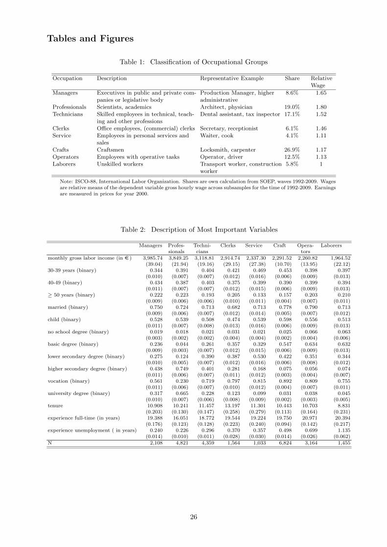
With respect to the choice of occupation, we distinguish eight groups of occupations relating

to the International Standard Classification of Occupation (ISCO-88).9 Table 1 summarizes

information on the classification of occupations including common examples for each group as

well as the share of each group within the sample. The listed groups of occupation provide

a distinction with respect to skill level and tasks. Therefore, a higher degree of homogeneity

is achieved submitting a more precise interpretation of returns to non-cognitive skills within

occupational groups.

[Include Table 1 here]

Moreover, the classification used can be related to the institutional system of occupational

training in Germany: While managers and professionals mostly require an academic education,

technicians correspond to the highest form of non-academic training. Below that we find typical

qualified jobs that require an apprenticeship including classroom education and practical train-

ing. This group is then divided into different tasks and can be found in occupational groups

clerks, service and craft. The group of operators comprises jobs that require only a short prac-

8Since individuals are not required to be at least 30 years when choosing their occupation, we rely on rank-orderstability only when measuring the impact of personality on occupational choice.

9The group of agricultural employees is not considered separately. Due to the small number they are eithercounted in the group of technicians or in the group of laborers depending on the level of required training.

7

tical training and no specific apprenticeship (e.g. a driver needs a licence). Finally, laborers do

not need any training.

Since the analysis covers a time span of 18 years, individuals are possibly observed in different

groups of occupation over time. There is a total number of 4,496 changes the we observe whereby

the number of ins and outs is not the same within each occupation. For instance, we do not

observe people leaving the group of laborers, but people starting to work as a laborer. On

average, 264 individuals per year switch their group of occupation. Analyzing ins and outs

for each occupational group reveals that the average probability of being observed in the same

group in two subsequent years is fairly high but varies across groups. It is lowest for managers

(65%) and highest for professionals and craftsmen (82 to 85%). Assuming a constant switching

propensity over the years, these differences do not influence our analysis since we run separate

estimations by occupation. Any possible unique effects that cannot be attributed to occupation

are then captured by the year dummies.

The main variable of interest is earnings. It is measured as the log of gross hourly wages. This

variable (subsequently simply referred to as wage) has been constructed by dividing monthly

gross labor income10 by actual weekly hours worked times 4.29 for the average number of weeks

per month. Using actual hours worked results in including overtime so that hourly wage rates

deviate from those indicated in the employment contract. Since we analyze a long time period,

we adjust wages for inflation by measuring them all in prices of the year 2000. To correct for

outliers we trim the upper and lower 2% of the distribution across all employees. The relative

wage figures indicate a wide spread of wages across occupations and all mean wages differ

significantly from the mean wage for laborers.

[Include Table 2 here]

The sample means (see Table 2) reveal a very homogenous picture with respect to the level

of formal education within groups of occupation and across genders. This, however, originates

in the classification which to a large part was chosen according to required skill level. Clearly,

managers, professionals, and technicians exhibit a much higher proportion of individuals having

higher secondary education or a university degree. Vice versa, there are less people without a

degree at all in these groups. Considering weekly working hours, professions requiring higher

formal education, on average, exhibit more weekly working hours.

Referring to the personality facets, comparisons across occupations are possible since units of

10Gross labor income includes overtime premiums but no special payments like e.g. leave pay.

8

measurement for the non-cognitive skills are the same in all groups of occupations. Gibbons et al.

(2005, p. 686) state that “if unmeasured skills are to explain estimated sector wage differentials,

then these skills must be non-randomly allocated across sectors”. That is to say that comparing

the distributions of non-cognitive skills across occupations should reveal distinct distributions if

the scores are standardized for all workers. Figures A-1 and A-2 (see Appendix A) display kernel

density estimates of the distributions of personality traits across occupations. Conscientiousness,

openness, reciprocity, and locus of control display the highest degree of variation. However, an

eye-ball check of the estimated kernel density is likely to veil existing differences. Running

mean comparison tests for all possible combinations of groups on average offered a rejection of

the null (equal means) in about 87% of the cases. Rejection rates were highest for openness,

extraversion and locus of control, and lowest for agreeableness.11 Overall, this presents solid

evidence for different distributions of non-cognitive skills across occupations. To what extent

these existing differences will also explain occupational sorting and wage differentials, will be

analyzed below.

4 Theoretical and Empirical Model

4.1 Theoretical Considerations

Following Gibbons et al. (2005) we model simultaneous determination of occupation and wages,

first of all assuming a unidimensional measure of non-cognitive skills that affects both outcome

variables. For sectors j = 1, ..., J , workers i = 1, ..., N , we model wages as

ln(yij) = Xiβj + ϑij , (1)

depending on exogenous variables denoted by matrix Xi that comprises information on socio-

economic background, job characteristics, regional information, and human capital variables like

level of education, labor market experience, or tenure. However, aspects of human capital that

are not as easily measurable, as for instance non-cognitive skills, are not included. Variables Xi

are assumed to be uncorrelated with the error term ϑij which can be decomposed as follows:

ϑij = νj + γjni + εij . (2)

It comprises non-cognitive skills ni that are valued differently (expressed by γj) in each occupa-

tional group j and an error term εij . Together they build a noisy signal of non-cognitive skills

11P-values of testing the hypothesis of equal means are displayed in detail in Table A-1 in Appendix A.

9

that is accompanied by an occupation specific constant νj . The error term εij has mean zero

and variance σ2ε and is assumed to be independent of the error terms of other occupations as

well as of the other variables Xi. Additional assumptions of zero costs to take up or end a job

are made.

Since ni is thought of as a one-dimensional measure of non-cognitive skills, sorting can be

modeled as follows. For increasing j more skilled labor is required and groups of occupations

remunerate ni increasingly with j. That is to say occupational groups can be seen as a hierarchy

that is defined by non-cognitive skills for given values of Xi. Assuming this order of groups

there exist critical values cj(Xi) that are strictly increasing in j. A worker with non-cognitive

skills ni will be assigned to occupation j if and only if

cj−1(Xi) < ni < cj(Xi) with c1(Xi) = −∞, cJ(Xi) = +∞, j = 1, ..., J, (3)

thus determining occupational sorting. This sorting results in wage differentials that can be ex-

plained by differences in the non-cognitive skill index for workers having the same Xi. Expected

wages increase with j as γj (price of skill measure in each occupational group) was assumed to

be strictly increasing in j and expected wages are

E[ln(yij)] = Xiβj + γjni + νj . (4)

Therefore E[ln(yij)] < E[ln(yi,j+1)] for fixed Xi indicating wage differentials solely due to differ-

ent non-cognitive skills.

Assuming a one-dimensional skill measure is a simplified model. For a more general model

we employ the M measures of non-cognitive skills. Consequently, occupational sorting can

be thought of being due to multidimensional non-cognitive skills. Critical values are replaced

subsequently by critical domains attributing a definition of the necessary range of each skill to

every group of occupation. For measures of non-cognitive skills m = 1, ...,M and groups of

occupation j = 1, ..., J , sorting occurs with respect to

cm,j−1(Xi) < nm,i < cm,j(Xi) with cm,1(Xi) = −∞, cm,J(Xi) = +∞. (5)

While some of the groups might have similar ranges for some of the skills, they can be distinct

with respect to particular skills. Every worker sorts into the occupation where the domain of

skills matches his or her non-cognitive skills.12

12Note that for overlapping domains for all measures of non-cognitive skills, an individual can sort into more

10

4.2 Estimation Approach

Occupational Choice

Sorting into occupations is estimated by a multinomial logit for J = 8 groups of occupations,

M = 7 measures of non-cognitive skills and N individuals.13 Assuming permanence of non-

cognitive skills, we can pool observations and the corresponding probability for each occupation

can then be estimated by:

Prob(occi = j|Zi,ni) = Pij =exp(Z′iβj + n′iγj)∑8j=1 exp(Z′iβj + n′iγj)

+ uij j = 1, ..., 8 i = 1, ..., N.

(6)

Error terms are assumed to be independently standard extreme value distributed. Estimating

a multinomial logit is only justified if independence of irrelevant alternatives (IIA) and thus

uncorrelated error terms of the alternatives can be assumed. Referring to the assumption of

independence of irrelevant alternatives, McFadden (1974, p. 113) states that “... application

of the model should be limited to situations where the alternatives can plausibly be assumed to

be distinct and weighed independently in the eyes of each decision-maker.” To assess whether

distinctness of alternatives is given, we conduct a Wald-test of whether groups of occupation can

be combined. The null hypothesis of interchangeability of groups was rejected for any possible

combination of groups and for all specifications of the multinomial logit. A rejection of the

Wald-tests thus underlines that the chosen groups of professions are independent of each other

which can be interpreted as evidence for the IIA to hold.14

Directly testing IIA applying Hausman-tests and Small-Hsiao-tests led to ambiguous results,

depending on specification and the test used. However, having evaluated different tests for IIA

with the help of simulation, Cheng and Long (2007) conclude that tests based on a restricted

choice set (including Hausman-test and Small-Hsiao test) are insufficient to support the IIA

assumption. Therefore, the ambiguous testing results do not speak against validity of IIA.

Exogenous variables Zi contain socio-economic characteristics, level of education, family

background (educational achievement and occupation of mother and father), regional variables

than one possible occupation.13There is a longstanding tradition to use a multinomial logit model to estimate occupational choice. Early

general applications of using a multinomial logit to estimate occupational attainment were provided by Boskin(1974) and Schmidt and Strauss (1975). Besides, the method has been applied to issues of occupational mobilityfor example of different ethnic minorities like in Kossoudji (1988) using the 1976 Survey of Income and Educationor Chiswick and Miller (2009) using US Census data from 2000. Cobb-Clark and Tan (2011) likewise employa multinomial logit model to the Australian HILDA data in order to estimate gender specific occupationalattainment. Besides, Constant and Zimmermann (2003) make use of a multinomial logit model for GermanSOEP data to estimate the influence of parents occupation on occupational choice of children.

14See Ham et al. (2009) who apply the same test to justify validity if IIA.

11

(dummies for geographical region, local unemployment rate, and regional GDP) and time dum-

mies while ni covers the measures of non-cognitive skills.15 Parents’ educational achievement

and occupation are included, since they offer important information with respect to occupa-

tional choice of individuals. As discussed in Card (1999), schooling outcomes of individuals

are highly correlated with family background which can be well described by attributes like

educational achievement and occupation of the parents. Schooling outcomes, in turn, are one of

the most important predictors of occupational choice as indicated above and by figures of Table

2 showing a distinct distribution of schooling levels across occupations. Furthermore, there is

also evidence that occupational choice is partly driven by occupational status of parents, see for

example Constant and Zimmermann (2003) or Chevalier (2002) for evidence of persistence in

choice of occupations over generations. Socio-economic characteristics and education capture

the fact that occupational groups vary with respect to attributes such as age. Occupations

requiring higher qualification are more likely to be held by older individuals due to the longer

training and the fact that labor does not play a role. Besides, education captures the distinctive

patterns of required qualification within occupational groups. Regional and time dummies are

intended to be a proxy for varying labor demand across groups.

To obtain the specification of the empirical model we started with a small model contain-

ing personality scores, educational variables, and socio-economic characteristics. Subsequently

groups of variables were added and their relevance was tested with the help of Wald tests.

Returns to Non-Cognitive Skills

The eight occupation-specific wage regressions are Mincer-type wage equations referring to the

natural log of gross hourly wages as the dependent variable. Conditional on group of occupation,

the dependent variable is explained using background variables X and measures of non-cognitive

skills n. The resulting coefficients of these scores, vector γ, are estimates of the returns to non-

15Socio-economic variables are dummy variables for German citizenship, presence of children younger than 16years, being married, and age coded into three dummy variables for being 40 to 49 years and 50 to 55 yearswith 30 to 39 years as the reference group. Regarding education, dummy variables for basic, lower secondary,and higher secondary education, possessing a vocational degree and having a university degree are included. Thereference group for education is no educational degree. Level of education of parents is also included in theanalysis, but here a coarser classification is applied: Dummy variables for possessing a lower secondary, highersecondary degree, or a university degree are coded for mother and father respectively. Parents’ occupation isregarded as well using the same classification as for the individuals included in the estimation. Hence, there areeight dummy variables for group of occupation for mother and father respectively. Regional information containslocal unemployment rates and GDP measured at the level of federal states and dummy variables for regions East,West, North, South, and city state. East comprises federal states Mecklenburg-Western Pomerania, Thuringia,Saxony, Saxony-Anhalt and Brandenburg. Region West corresponds to federal states North Rhine-Westphalia,Rhineland-Palatinate and Hesse. The northern region stands for federal states Schleswig-Holstein and LowerSaxony. South (the reference region) comprises federal states Bavaria and Baden-Wuerttemberg. City statescorrespond to federal city states Berlin, Hamburg and Bremen.

12

cognitive skills within a particular group of occupation.

ln(wagei|occi = j) = αi + X′iβ + n′iγ + εi, j = 1, ..., 8, i = 1, ..., N. (7)

For the wage equations we employ socio-economic characteristics, level of education, la-

bor market experience, job characteristics as well as region and time variables as background

variables besides the non-cognitive skills.16 Region and time variables are included to capture

differences in the level of remuneration across federal states and across business cycles. Labor

market experience is a proxy for productivity of employees and hence influences the wage rate.

Besides, job characteristics include productivity signals as well like the tenure of a person within

the firm or the level of required training for a specific job, but also general factors like the size

of the employing firm or an indicator for public sector employment. Related are the education

variables. They as well serve as a productivity signal. Parental education is not included since

it is not a direct determinant of individual earnings but instead has a mediating role via occupa-

tion. Since we estimate occupation-specific wage equations and because occupational groups are

relatively homogeneous with respect to the general level of education and training, the influence

of parental background is already taken into account. Finally, socio-economic characteristics

reflect the fact that increases in wages are often linked to aspects like family status or age, at

least if collective agreements are in place.

Again, we started with a small model containing personality scores, educational variables,

and socio-economic characteristics. Subsequently groups of variables were added to the model

and their relevance was tested with the help of Wald-tests.

5 Empirical Results

5.1 The Impact of Non-cognitive Skills on Occupational Choice

To explain choice of occupation, we have estimated a multinomial logit model using laborers as

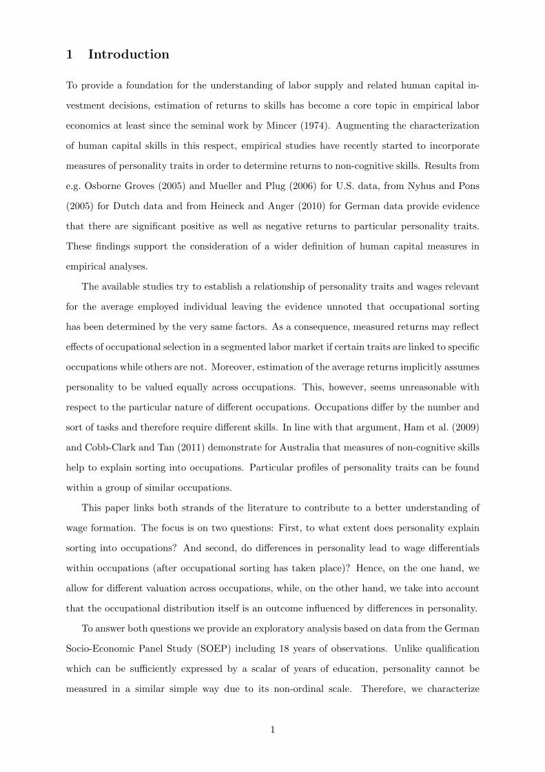
the baseline occupation.17 Figure 1 presents obtained average marginal effects. These refer to

changes in the probability to be observed in a particular group of occupation in case regressors

change, averaged across the sample.18 Concentrating on statistically significant marginal effects,

16Labor market experience is measured in quadratic polynomials of years spent in full-time and part-timeemployment as well as of years in unemployment. Job characteristics included are dummy variables for workingin the public sector and for being employed in a company with at least 200 employees. In addition, tenure andthe required training of the position held are considered. Required training is a dummy variable equal to one ifthe employment requires having a diploma from a university or a university of applied sciences.

17Laborers are the group with the lowest qualification requirements.18Table A-2 in the Appendix displays all estimated coefficients of the personality variables.

13

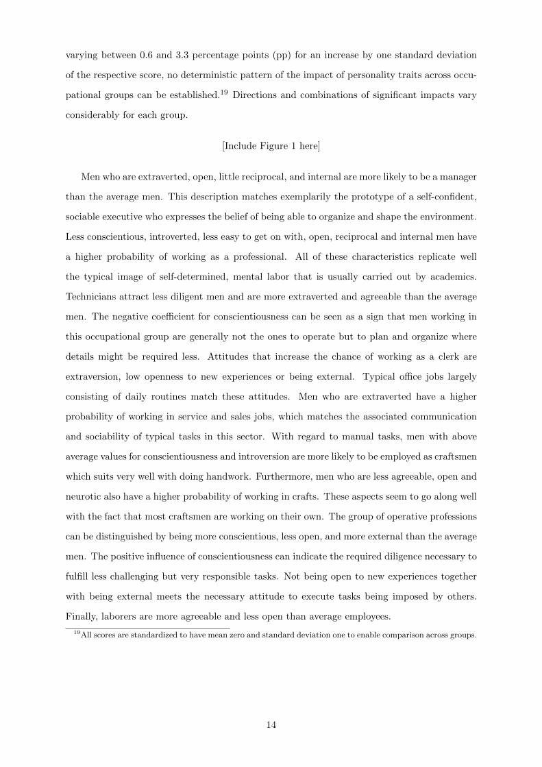
varying between 0.6 and 3.3 percentage points (pp) for an increase by one standard deviation

of the respective score, no deterministic pattern of the impact of personality traits across occu-

pational groups can be established.19 Directions and combinations of significant impacts vary

considerably for each group.

[Include Figure 1 here]

Men who are extraverted, open, little reciprocal, and internal are more likely to be a manager

than the average men. This description matches exemplarily the prototype of a self-confident,

sociable executive who expresses the belief of being able to organize and shape the environment.

Less conscientious, introverted, less easy to get on with, open, reciprocal and internal men have

a higher probability of working as a professional. All of these characteristics replicate well

the typical image of self-determined, mental labor that is usually carried out by academics.

Technicians attract less diligent men and are more extraverted and agreeable than the average

men. The negative coefficient for conscientiousness can be seen as a sign that men working in

this occupational group are generally not the ones to operate but to plan and organize where

details might be required less. Attitudes that increase the chance of working as a clerk are

extraversion, low openness to new experiences or being external. Typical office jobs largely

consisting of daily routines match these attitudes. Men who are extraverted have a higher

probability of working in service and sales jobs, which matches the associated communication

and sociability of typical tasks in this sector. With regard to manual tasks, men with above

average values for conscientiousness and introversion are more likely to be employed as craftsmen

which suits very well with doing handwork. Furthermore, men who are less agreeable, open and

neurotic also have a higher probability of working in crafts. These aspects seem to go along well

with the fact that most craftsmen are working on their own. The group of operative professions

can be distinguished by being more conscientious, less open, and more external than the average

men. The positive influence of conscientiousness can indicate the required diligence necessary to

fulfill less challenging but very responsible tasks. Not being open to new experiences together

with being external meets the necessary attitude to execute tasks being imposed by others.

Finally, laborers are more agreeable and less open than average employees.

19All scores are standardized to have mean zero and standard deviation one to enable comparison across groups.

14

5.2 Occupation-Specific Returns to Non-Cognitive Skills

The influence of personality traits on wages consists of occupation-specific combinations of

significant effects, confirming our expectation of heterogeneity of returns (see Figure 2 and Table

A-3 in the Appendix for full estimation results). Overall, returns to non-cognitive skills range

from -4.6 to +2.9% in case a particular score changes by one standard deviation. The absolute

effect size is close to estimates of the returns to an additional year of schooling which usually

range from 5 to 8%20 showing the considerable influence of non-cognitive skills in explaining

wages. Moreover, some traits exhibit a clear pattern across occupations: Agreeableness and

locus of control display negative returns across most occupational groups, albeit the sizes of

the effects differ. These patterns are not surprising, given the associated behavior of the traits:

A high level of agreeableness is mainly associated with the need for a harmonious and kind

atmosphere while for executive jobs within each of the occupational groups this attitude is

rather not desired. And an external (high) locus of control expresses the belief that one has only

humble influence on outcomes. Both characteristics are unlikely to foster advancement within

occupational hierarchies which are related to higher earnings. Beyond that, conscientiousness,

openness and reciprocity exhibit significant returns in some of the occupations. With regard

to these subtleties, a model estimating returns to non-cognitive skills for the average employee

can veil occupational heterogeneity.

[Include Figure 2 here]

According to Figure 2, the following personality profiles earn highest within each occupa-

tion: Managers report higher earnings the more unkind and internal they are, which can be

interpreted as a possible indicator for decisiveness. Professionals are rewarded when being in-

ternal reflecting the need to organize one’s workload self-determinedly. Technicians earn more,

the less conscientious, agreeable, and external they are. The negative effect of conscientiousness

possibly relates to a correlation of hierarchy and the ability to be proactive. Clerks as well

have higher wages when being less agreeable and external than the average clerk showing a

similar profile to managers but with different sizes of the effects: While managers experience

a larger wage penalty for agreeableness than for being external, the reverse is true for clerks.

Service workers earn highest when being internal. Craftsmen have higher wages if they exhibit

below-average conscientiousness and an internal attitude. Since their work can be characterized

as highly discretionary, being external or overly conscientious appears rather obstructive to pro-

20See Card (1999) for a summary of empirical findings (table 6, p. 1849-1850).

15

fessional advancement. Operators with high wages exhibit low conscientiousness, agreeableness

as well as high openness and reciprocity. Here one could suspect that the only possibility to be

promoted (and earn more) as an operator is to become foreman, a task where the attitudes just

describes appear suitable. Finally, laborers earn most when being little agreeable, but open

to experience and reciprocal. Hence, a similar reward structure as for operators applies. In

absolute terms the returns presented account for observable earnings differences ranging from

e20 to e125 with respect to single personality traits.21

While evaluating returns to non-cognitive skills, it is of interest whether attitudes that

increased the employment probability in a particular occupation are any longer favorable or

play a different role, once a person became employed. If a trait displays the same impact on

both outcomes, a strong demand for the specific skill might be driving the results. An example

for effects with the same sign within one group but for both outcomes is locus of control for

managers. If however, a trait increases the employment probability but lowers wages once

employed, possibly only a certain range of values is favored. While values beyond this interval

could serve as a signal in the first stage, they could be penalized in the second one. Moreover,

some attitudes that are positively linked to employment in a particular group of occupation

can be highly correlated with positions in the lower part of the hierarchy thereby resulting in

lower wages. A third possible explanation is that the preference to work in a specific professional

group is very high: Individuals then accept lower wages because the utility of that specific group

compensates them for the wage loss due to non-cognitive skills. Effects working in the opposite

directions with respect to both outcomes can be observed for technicians and the agreeableness

facet.

5.3 Returns to Different Types of Personality

Interpretation of the marginal effects provided so far requires the assumption that a ceteris-

paribus evaluation of a single personality trait is meaningful. It is, however, hard to imagine

why a specific aspect of personality should change, especially when the other traits remain

unchanged. In addition, changes in personality have been shown to be small (see Cobb-Clark

and Schurer, 2011b, 2011a). Thus, it seems more encouraging and relevant to compare returns

to different types of personality rather than changes of specific attitudes.

To construct measures for joint appearance of certain traits (subsequently denoted as per-

21We apply a back-of-the-envelope calculation, where marginal effects are multiplied with the average wagerate in the sample times 4.29 (average number of weeks per month) times 40 (assuming full-time employment of40 hours per week). Earnings are measured in prices of the year 2000.

16

sonality types or profiles) we assess whether an individual’s score for a trait is either lower than

the median value or greater equal to it.22 This approach is not intended to construct stereotypes

but an attempt to capture and classify possible patterns of personality as well as correlations

between traits.23 To restrict the number of possible combinations, we limit the analysis to the

Big Five traits (that intend to provide a complete mapping of an individual’s personality) leav-

ing us with 25 = 32 possible combinations. Table 3 displays these types together with the

corresponding shares in our sample.

[Include Table 3 here]

Using indicators for these personality types instead of single trait measures allows to analyze

the joint impact of a personality profile and thereby to capture the large amount of heterogeneity

in the distribution of personality traits. Moreover, evaluation of personality profiles incorporates

possible non-linearities in the impact of personality on earnings: An implicit assumption when

estimating returns to personality using single scores of traits is that the impact is linear. This

assumption is avoided here since the joint impact of traits is evaluated compared to a reference

profile.

We rely on the most frequently occurring type within the sample, that is characterized by

having above-median values for the traits conscientiousness, extraversion, agreeableness and

openness to experience, in combination with below-median values for neuroticism (Type 2).24

Evaluation will be concentrated on the largest two occupational groups which are craft and

professionals. Figure 3 summarizes marginal effects of returns to personality profiles for these

particular groups.25

[Include Figure 3 here]

The lighter-shaded bars in Figure 3 refer to craftsmen and show that compared to Type 2

personality, there are five personality profiles that display significantly deviating wages within

the group of craftsmen. First, men who have above-median values for all of the Big Five traits

22Swope et al. (2008) undertake a similar analysis to classify interaction of certain traits: Using the Meyer-Briggs-typology they describe relative frequencies of types built as joint appearance of four attitudes.

23Albeit orthogonal factor rotation, which is used to construct measures of non-cognitive skills, by definitioncreates uncorrelated measures, loadings on more than one factor de facto lead to correlated factors. Correlationanalysis for the Big Five personality traits within our sample reveals a negative relationship between neuroticismand the other four traits. Conscientiousness and agreeableness as well as extraversion are substantially positivelycorrelated. The same applies for extraversion and openness to experience. These relationships can be found inother samples, too, see Biesanz and West (2004).

24This personality profile accounts for around 8.5% of the sample. Assuming a uniform distribution, eachtype would occur with a share of 3.125%. A share of 8.5% thus represents an almost threefold more probableoccurrence of that specific type.

25Marginal effects for all personality types are displayed in Appendix A in Table A-4.

17

except for openness (Type 3) on average earn 8.6% less than men with the comparison profile.

Second, men who have above-median values for all of the Big Five traits with the exception

of extraversion (Type 9) also experience a negative effect of about 6% compared to men with

a personality profile of Type 2. Third, men with above-median values for conscientiousness,

agreeableness and openness but below-median values for extraversion and neuroticism (Type

10) report on average roughly 9% lower wages. Fourth, compared to Type 2 there is a wage

premium of about 7% for men with below-median values for all of the Big Five traits except for

conscientiousness (Type 16). And finally, men with above-median values for all of the big Five

traits except for conscientiousness (Type 17), that is the “opposite” of Type 16, earn about 11%

less. Given that craftsmen with Type 2 personality profile on average report monthly wages of

e1,990, the deviations of men with other profiles lead to monthly earnings differences ranging

from about e-225 for Type 17 to about e+130 for Type 16.26

Wage differences across personality types for professionals, the second largest occupational

group, are displayed by the black bars in Figure 3. Notably, all effects are positive which means

that individuals with a personality profile of Type 2 earn equal or less than all other profiles

considered. Since the number of significant effects is larger than for the group of craftsmen we

will concentrate on the effects for the five types with the largest shares. First of all, men that

are characterized by Type 12 (high on conscientiousness and agreeableness, low on the other

three traits) exhibit an average wage premium of about 9% when compared to Type 2 who

additionally has high scores for extraversion and openness. Second, professionals with below-

median values of conscientiousness and neuroticism but above-median values of the other traits

(Type 18) on average earn 8% more than the comparison group. For Type 28 (above-median

values for agreeableness, all other traits are below the respective median), the wage premium

with respect to Type 2 is already 10%. Finally, personality types 31 and 32 display a ca. 8%

higher wage than professionals with Type 2 personality. Applying the same back-of-the-envelope

calculation as above this corresponds to absolute wage premiums of about e180-230.

Beyond the examples provided, results for the other occupational groups reveal large het-

erogeneity with respect to the personality profile. Among the 31 Types analyzed, the ones

that show significantly different wages differ with occupational group without a clear pattern

confirming our finding that returns are occupation-specific.

26We apply a back-of-the-envelope calculation, where marginal effects are multiplied with the average wagerate in the sample times 4.29 (average number of weeks per month) times 40 (assuming full-time employment of40 hours per week). Earnings are measured in prices of the year 2000.

18

5.4 Robustness Checks

Given the heterogeneity of the impact of personality measures on occupational choice, individ-

ual occupation can be doubted to be exogenous when analyzing occupation-specific returns to

personality. We have therefore estimated selection-corrected returns according to Bourguignon

et al. (2007) who model selection based on a multinomial logit model.27 The selection-corrected

results are displayed in Table A-5 in Appendix A. Comparing them with those from OLS pre-

sented in Table A-3 reveals partly diverging results indicating that there is some selection-bias.

However, the general pattern from the OLS results is replicated and none of these effects van-

ishes. Instead, we find more and larger significant returns to personality traits with the selection

correction method. Moreover, there are now opposing effects for openness and reciprocity across

occupational groups indicating an even larger heterogeneity of returns with respect to occupa-

tion. Therefore we suppose that the results presented in section 5.2 are robust and represent a

cautious estimation of the relationship between personality traits and occupation-specific wages.

Another issue that we consider is that personality traits are measured with error which

leads to an attenuation bias (see e. g. Greene, 2008) that make our estimates a lower bound

of the true relationship. Application of errors-in-variables estimation that accounts for the

reliability of the trait measures confirms that agreeableness and locus of control are the most

important personality traits.28 Furthermore, it results in larger estimated coefficients (see Table

A-6 in Appendix A for the estimation results), thus confirming the attenuation hypothesis.

Nevertheless, some of the significant results from the OLS estimation are now insignificant

while others are added. These robustness checks confirm our general result of occupation-

specific returns to personality. Beyond that they indicate that the specific coefficients reveal

some sensitivity with respect to the evaluation method used.

6 Conclusion

We have analyzed the role of personality in occupational choice and wage formation, linking

both aspects. Personality has been captured by the use of seven different traits. The empirical

results for choice of occupation indicate that a ceteris paribus change in the score of a single

trait by one standard deviation leads to changes in the probability of working in a specific

occupational group by about 7 to 24%. This strongly supports Holland’s idea (Holland, 1966)

that individuals sort into occupations due to interests which are driven by personal attitudes.

27The theoretical model as well as the estimation equation is presented in Appendix C.28As a measure for the reliability we use Cronenbach’s Alpha.

19

Whether the differences in personality traits across occupations are mainly caused by selective

applications from the employee’s side or by selective recruitment from the employer’s side cannot

be determined within a reduced form model. Nevertheless, the information conveyed in the

estimation of personality influences on both outcome variables differs. During the placement

process employers are faced with a large diversity of applicants. Hence, the final choice of

employees contains a lot of information on which personality traits are favored. Regarding

the stage of wage determination, we observe a group of employees that differ much less than

applicants. Holland (1966, p. 287) describes this aspect as classifying “people having similar

vocational choices”... means “classifying similar personalities together”. Returns to wages, on

the one hand, can then be seen as rating the excess differences in personality existing between

employees. On the other hand, they may express the demand for further characteristics that

could not be fulfilled during the stage of selecting employees.29

The results of the occupation-specific returns to personality show that the patterns of sig-

nificant effects for the seven traits considered vary across occupational groups. Agreeableness

and locus of control are the most important personality traits with respect to wages, while con-

scientiousness and reciprocity play only a minor role. In contrast to the results for occupational

choice, the signs of the coefficients are now (mostly) identical across occupations. Returns range

from -4.5% to +2.9% wage changes in case the trait measure increases by one standard devia-

tion. Translated into absolute numbers by a back-of-the-envelope calculation, where marginal

effects are multiplied with the average wage rate in the sample times 4.29 (average number of

weeks per month) times 40 (assuming full-time employment of 40 hours per week), results in

absolute earnings differentials of about e20 to e125 in gross monthly income with respect to

single traits (using average currency values for the pooled sample from 1992 to 2009 measured

in prices of 2000).

The occupation-specific heterogeneity found can help to explain contradictory results of

previous work. Mueller and Plug (2006) for example conclude that men profit from higher

scores for openness to experience, whereas Heineck and Anger (2010) estimate negative returns

for higher scores of openness. A possible explanation is that there are differences with respect

to the occupational distribution of the sample that translate into different estimates. But

importantly, our findings are in line with prior evidence that non-cognitive skills in fact play a

29Estimating the relationship of personality and earnings assumes that there is no correlation with other factorsinfluencing returns as for example cost of effort. Estimates therefore can only provide gross effects since thesefactors are unmeasurable and are likely correlated with personality traits. Besides, returns to non-cognitiveskills may interfere with compensating wage differentials that measure wage premiums for specific (adverse)characteristics of the employment.

20

role in determining wages. Controlling for occupation, hence comparing like with like, we still

find significant returns to non-cognitive skills indicating that wage differentials due to different

personality traits are not solely transmitted via occupational choice but constitute inherent

rewards to skills. Several robustness checks confirm this finding albeit the exact results differ

somehow with the method applied.

Beyond ceteris paribus analysis of marginal effects we analyze returns to personality types

constructed as combinations of low and high values for the Big Five traits instead of single

traits. This allows to capture heterogeneity in the distribution of traits, correlation of traits, as

well as nonlinearity of the impact of personality. Employing indicators of these types instead

of the scores for the single traits in the regression shows a distinct distribution of earnings

across types. Switching from a baseline type who displays above-median values for the traits

conscientiousness, extraversion, agreeableness, and openness to experience, as well as below-

median values for neuroticism, to other types induces wage changes of about -18 to +17%

confirming our heterogeneity result with respect to personality returns. Again using the back-

of-the-envelope calculation this translates into absolute monthly earnings differentials of up to

e230 between men with different personality profiles.

We have shown that there is an interdependency of personality, occupation and wages which

underlines the importance of an occupation-specific evaluation of returns since personality is

valued differently in each group even when controlling for a large variety of human capital and

other background variables. In the light of policies aiming at the allocation of labor supply our

findings provide an insight regarding the quality of possible matches.

References

Biesanz, J.C., West, S.G., 2004. Towards understanding assessment of the Big Five: Multitrait-

multimethod analyses of convergent and discriminant validity across measurement occasion

and type of observer. Journal of Personality 72, 845–876.

Borghans, L., ter Weel, B., Weinberg, B.A., 2008. Interpersonal styles and labor market out-

comes. Journal of Human Resources 43, 815–858.

Boskin, M.J., 1974. A conditional logit model of occupational choice. The Journal of Political

Economy 82, 389–398.

Bourguignon, F., Fournier, M., Gurgand, M., 2007. Selection bias correction based on the

21

multinomial logit model: Monte Carlo comparisons. Journal of Economic Surveys 21, 174–

205.

Bowles, S., Gintis, H., Osborne, M., 2001b. The determinants of earnings: A behavioral ap-

proach. Journal of Economic Literature 29, 1137–1176.

Card, D., 1999. Causal effects of education on earnings, in: Ashenfelter, O., Card, D. (Eds.),

Handbook of Labor Economics. Elsevier Science B.V.. chapter 30, pp. 1801–1863.

Cheng, S., Long, J.S., 2007. Testing for IIA in the multinomial logit model. Sociological Methods

and Research 35, 583–600.

Chevalier, A., 2002. Just like daddy: The occupational choice of UK graduates, Royal Economic

Society Annual Conference. Royal Economic Society.

Chiswick, B.R., Miller, P.W., 2009. Earnings and occupational attainment among immigrants.

Industrial Relations 48, 454–465.

Cobb-Clark, D., Schurer, S., 2011a. The Stability of Big-Five Personality Traits. Discussion

Paper 5943. Institute for the Study of Labor (IZA). Bonn.

Cobb-Clark, D., Schurer, S., 2011b. Two Economists’ Musings on the Stability of Locus of

Control. Discussion Paper 5630. Institute for the Study of Labor (IZA). Bonn.

Cobb-Clark, D.A., Tan, M., 2011. Non-cognitive skills, occupational attainment, and relative

wages. Labour Economics 18, 1–13.

Constant, A.F., Zimmermann, K.F., 2003. Occupational choice across generations. Applied

Economics Quarterly 49, 299–317.

Costa, Jr., P.T., McCrae, R.R., 1988. Personality in adulthood: A six-year longitudinal study

of self-reports and spouse ratings on the NEO personality inventory. Journal of Personality

and Social Psychology 54, 853–863.

Cunha, F., Heckman, J.J., 2007. The technology of skill formation. American Economic Review

97, 31–47.

Dubin, J.A., McFadden, D.L., 1984. An econometric analysis of residential electric appliance

holdings and consumption. Econometrica 52, 345–362.

22

Filer, R.K., 1986. The role of personality and tastes in determining occupational structure.

Industrial and Labor Relations Review 39, 412–424.

Gerlitz, J.Y., Schupp, J., 2005. Zur Erhebung der Big-Five-basierten Personlichkeitsmerkmale

im SOEP. Research Note 4. DIW. Berlin.

Gibbons, R., Katz, L.F., Lemieux, T., Parent, D., 2005. Comparative advantage, learning and

sectoral wage determination. Journal of Labor Economics 23, 681–723.

Greene, W.H., 2008. Econometric Analysis. Pearson.

Guilford, J.S., Zimmerman, W.S., Guilford, J.P., 1976. The Guilford-Zimmerman Temperament

Survey Handbook : Twenty-Five Years Research and Applications. EdITS Publishers, San

Diego, California.

Ham, R., Junankar, P.R., Wells, R., 2009. Antagonistic Managers, Careless Workers and Ex-

traverted Salespeople: An Examination of Personality in Occupational Choice. Discussion

Paper 4193. Institute for the Study of Labor (IZA). Bonn.

Heckman, J.J., Stixrud, J., Urzua, S., 2006. The effects of cognitive and noncognitive abilities

on labor market outcomes and social behavior. Journal of Labor Economics 24, 411–482.

Heineck, G., Anger, S., 2010. The returns to cognitive abilities and personality traits in Ger-

many. Labour Economics 17, 535–546.

Holland, J.L., 1966. A psychological classification scheme for vocations and major fields. Journal

of Counseling Psychology 13, 278–288.

Jacobson, J.P., 1999. Labor force participation. The Quarterly Review of Economics and

Finance 39, 597–610.

Johnson, J.A., 2000. Units of analysis for the description and explanation of personality, in:

Hogan, R., Johnson, J., Briggs, S. (Eds.), Handbook of Personality Psychology. Academic

Press. chapter 3, pp. 73–93.

Judge, T.A., Higgins, C.A., Thoresen, C.J., Barrick, M.R., 1999. The Big Five personality

traits, general mental ability, and career success across the life span. Personnel Psychology

52, 621–652.

Kossoudji, S.A., 1988. English language ability and the labor market opportunities of Hispanic

and East Asian immigrant men. Journal of Labor Economics 6, 205–228.

23

Krueger, A.B., Schkade, D., 2008. Sorting in the labor market: Do gregarious workers flock to

interactive jobs? Journal of Human Resources 43, 861–885.

McCrae, R.R., John, O.P., 1992. An introduction to the Five-Factor Model and its application.

Journal of Personality 60, 175–215.

McFadden, D.L., 1974. Conditional logit analysis of qualitative choice behavior, in: Zarembka,

P. (Ed.), Frontiers in Econometrics. Academic Press, New York. chapter 4, pp. 105–142.

Mincer, J., 1974. Schooling, Experience, and Earnings. Columbia University Press.

Mueller, G., Plug, E., 2006. Estimating the effect of personality on male and female earnings.

Industrial and Labor Relations Review 60, 3–22.

Nyhus, E.K., Pons, E., 2005. The effect of personality on earnings. Journal of Economic

Psychology 26, 363–384.

Osborne Groves, M., 2005. How important is your personality? Labor market returns to

personality in the US and UK. Journal of Economic Psychology 26, 827–841.

Piatek, R., Pinger, P., 2010. Maintaining (Locus of) Control? Assessing the Impact of Locus of

Control on Education Decisions and Wages. Discussion Paper 5289. Institute for the Study

of Labor (IZA). Bonn.

Rabin, M., 1993. Incorporating fairness into game theory and economics. American Economic

Review 83, 1281–1302.

Roberts, B.W., DelVecchio, W.F., 2000. The rank-order consistency of personality traits from

childhood to old age: A quantitative review of longitudinal studies. Psychological Bulletin

126, 3–25.

Roberts, B.W., Walton, K.E., Viechtbauer, W., 2006. Patterns of mean-level change in per-

sonality traits across the life course: A meta-analysis of longitudinal studies. Psychological

Bulletin 132, 1–25.

Robins, R.W., Fraley, R.C., Roberts, B.W., Trzesnewski, K.H., 2001. A longitudinal study of

personality change in young adulthood. Journal of Personality 69, 617–640.

Rotter, J.B., 1966. Generalized Expectancies for Internal versus External Control of Reinforce-

ment. American Psychological Association, Washington, DC.

24

Rotter, J.B., 1975. Some problems and misconceptions related to the construct of internal

versus external control of reinforcement. Journal of Consulting and Clinical Psychology 43,

56–67.

Schmidt, P., Strauss, R.P., 1975. The prediction of occupation using multiple logit models.

International Economic Review 16, 471–486.

Stevens, C.K., Bavetta, A.G., Gist, M.E., 1993. Gender differences in the acquisition of salary

negotiation skills: The role of goals, self-efficacy, and perceived control. Journal of Applied

Psychology 78, 723–735.

Swope, K.J., Cadigan, J., Schmitt, P.M., Shupp, R., 2008. Personality preferences in laboratory

economics experiments. Journal of Socio-Economics 37, 998–1009.

Terracciano, A., Costa, Jr., P.T., McCrae, R.R., 2006. Personality plasticity after age 30.

Personality and Social Psychology Bulletin 32, 999–1009.

Wagner, G.G., Frick, J.R., Schupp, J., 2007. The German Socio-Economic Panel Study (SOEP)

- scope, evolution and enhancements. Schmollers Jahrbuch 127, 139–169.

25

Tables and Figures

Table 1: Classification of Occupational Groups

Occupation Description Representative Example Share RelativeWage

Managers Executives in public and private com-panies or legislative body

Production Manager, higheradministrative

8.6% 1.65

Professionals Scientists, academics Architect, physician 19.0% 1.80Technicians Skilled employees in technical, teach-

ing and other professionsDental assistant, tax inspector 17.1% 1.52

Clerks Office employees, (commercial) clerks Secretary, receptionist 6.1% 1.46Service Employees in personal services and

salesWaiter, cook 4.1% 1.11

Crafts Craftsmen Locksmith, carpenter 26.9% 1.17Operators Employees with operative tasks Operator, driver 12.5% 1.13Laborers Unskilled workers Transport worker, construction

worker5.8% 1

Note: ISCO-88, International Labor Organization. Shares are own calculation from SOEP, waves 1992-2009. Wagesare relative means of the dependent variable gross hourly wage across subsamples for the time of 1992-2009. Earningsare measured in prices for year 2000.

Table 2: Description of Most Important Variables

Managers Profes-sionals

Techni-cians

Clerks Service Craft Opera-tors

Laborers

monthly gross labor income (in e ) 3,985.74 3,849.25 3,118.81 2,914.74 2,337.30 2,291.52 2,260.82 1,964.52(39.04) (21.94) (19.16) (29.15) (27.38) (10.70) (13.95) (22.12)

30-39 years (binary) 0.344 0.391 0.404 0.421 0.469 0.453 0.398 0.397(0.010) (0.007) (0.007) (0.012) (0.016) (0.006) (0.009) (0.013)

40-49 (binary) 0.434 0.387 0.403 0.375 0.399 0.390 0.399 0.394(0.011) (0.007) (0.007) (0.012) (0.015) (0.006) (0.009) (0.013)

≥ 50 years (binary) 0.222 0.223 0.193 0.205 0.133 0.157 0.203 0.210(0.009) (0.006) (0.006) (0.010) (0.011) (0.004) (0.007) (0.011)

married (binary) 0.750 0.724 0.713 0.682 0.713 0.778 0.790 0.713(0.009) (0.006) (0.007) (0.012) (0.014) (0.005) (0.007) (0.012)

child (binary) 0.528 0.539 0.508 0.474 0.539 0.598 0.556 0.513(0.011) (0.007) (0.008) (0.013) (0.016) (0.006) (0.009) (0.013)

no school degree (binary) 0.019 0.018 0.021 0.031 0.021 0.025 0.066 0.063(0.003) (0.002) (0.002) (0.004) (0.004) (0.002) (0.004) (0.006)

basic degree (binary) 0.236 0.044 0.261 0.357 0.329 0.547 0.634 0.632(0.009) (0.003) (0.007) (0.012) (0.015) (0.006) (0.009) (0.013)

lower secondary degree (binary) 0.275 0.124 0.390 0.387 0.530 0.422 0.351 0.344(0.010) (0.005) (0.007) (0.012) (0.016) (0.006) (0.008) (0.012)

higher secondary degree (binary) 0.438 0.749 0.401 0.281 0.168 0.075 0.056 0.074(0.011) (0.006) (0.007) (0.011) (0.012) (0.003) (0.004) (0.007)

vocation (binary) 0.561 0.230 0.719 0.797 0.815 0.892 0.809 0.755(0.011) (0.006) (0.007) (0.010) (0.012) (0.004) (0.007) (0.011)

university degree (binary) 0.317 0.665 0.228 0.123 0.099 0.031 0.038 0.045(0.010) (0.007) (0.006) (0.008) (0.009) (0.002) (0.003) (0.005)

tenure 10.908 10.241 11.457 13.197 11.301 10.443 10.703 8.831(0.203) (0.130) (0.147) (0.258) (0.279) (0.113) (0.164) (0.231)

experience full-time (in years) 19.388 16.051 18.772 19.544 19.224 19.750 20.971 20.394(0.176) (0.123) (0.128) (0.223) (0.240) (0.094) (0.142) (0.217)

experience unemployment ( in years) 0.240 0.226 0.296 0.370 0.357 0.498 0.699 1.135(0.014) (0.010) (0.011) (0.028) (0.030) (0.014) (0.026) (0.062)

N 2,108 4,821 4,359 1,564 1,033 6,824 3,164 1,455

26

Figure 1: Marginal Effects of Personality on Occupational Choice

Note: Own calculation from SOEP. Displayed are marginal effects at the mean: ∂Pij/∂x indicating percentage point

changes in the probability to be observed in a particular group of occupations in case a personality score increases by one

standard deviation. All effects are significant at the 10% level (or stricter). For full estimation results see Table A-2 in

Appendix A.

Further variables included in the estimation: age; married; child; German; basic, lower secondary, higher secondary

education; vocational degree; university degree; lower secondary, higher secondary education, university degree of mother

and father; dummies for occupations groups 1-8 for father and mother; unemployment rate and GDP at state level; east,

west, north, city-state; year 1992-2008.

Table 3: Definition and Shares of Personality Types Built from Big Five Traits

C E A O N Share C E A O N Share

Type 1 + + + + + 3.71% Type 17 - + + + + 2.18%

Type 2 + + + + - 8.43% Type 18 - + + + - 3.80%

Type 3 + + + - + 2.10% Type 19 - + + - + 1.48%

Type 4 + + + - - 3.95% Type 20 - + + - - 2.87%

Type 5 + + - + + 1.98% Type 21 - + - + + 3.13%

Type 6 + + - + - 2.71% Type 22 - + - + - 2.32%

Type 7 + + - - + 1.61% Type 23 - + - - + 2.33%

Type 8 + + - - - 1.87% Type 24 - + - - - 2.74%

Type 9 + - + + + 2.12% Type 25 - - + + + 2.38%

Type 10 + - + + - 3.16% Type 26 - - + + - 2.72%

Type 11 + - + - + 3.18% Type 27 - - + - + 3.81%

Type 12 + - + - - 4.24% Type 28 - - + - - 4.56%

Type 13 + - - + + 1.81% Type 29 - - - + + 3.08%

Type 14 + - - + - 1.45% Type 30 - - - + - 2.03%

Type 15 + - - - + 2.94% Type 31 - - - - + 8.16%

Type 16 + - - - - 2.44% Type 32 - - - - - 4.69%

Note: Own calculation from SOEP. C=Conscientiousness, E=extraversion, A=agreeableness,O=openness, N=neuroticism. “+”= trait value equal to or above median, “-”= trait value be-low median.

27

Figure 2: Marginal Effects of Personality on Occupation-Specific Wages

‐0.01

0.01

0.03

Managers Professionals Technicians Clerks Service Craft Operators Laborers

‐0.07

‐0.05

‐0.03

Conscientiousness Extraversion Agreeableness Openess Neuroticism Reciprocity Control

Note: Own calculation from SOEP. Displayed are significant coefficients (10% level or stricter) after estimation of Equation

7 with gross hourly wage as dependent variable indicating the percentage change in wages in case a personality score

increases by one standard deviation. Standard errors are robust and account for clustering at the person level. See Table

A-3 in Appendix A for full estimation results.

Further variables included in the estimations: age; married; child; German; basic, lower secondary, higher secondary edu-

cation; vocational degree; university degree; experience and experience squared in full-time, part-time and unemployment;

firm with at least 200 employees; public employer; required training; tenure; unemployment rate and GDP at state level;

east, west, north, city-state; year 1992-2008.

28

Figure 3: Marginal Effects of Personality Profiles on Wages of Craftsmen and Professionals

0

0.02

0.04

0.06

0.08

0.1

0.12

0.14

0.16

0.18

‐0.12

‐0.1

‐0.08

‐0.06

‐0.04

‐0.02

0

1 2 3 4 5 6 7 8 9 10 11 12 13 14 15 16 17 18 19 20 21 22 23 24 25 26 27 28 29 30 31 32

Professionals Craft

Note: Own calculation from SOEP. Displayed are significant coefficients (10% level or stricter) after estimation of Equation

7 with gross hourly wage as dependent variable accounting for robust standard errors and clustering at the person level.

Effects indicate the percentage change in wages in case that an individual is observed having Type X personality profile

instead of Type 2 (the baseline). See Table A-4 in Appendix A for full estimation results.

Further variables included in the estimations: age; married; child; German; basic, lower secondary, higher secondary edu-

cation; vocational degree; university degree; experience and experience squared in full-time, part-time and unemployment;

firm with at least 200 employees; public employer; required training; tenure; unemployment rate and GDP at state level;

east, west, north, city-state; year 1992-2008.

29

Appendix

A Further Tables and Figures

Table A-1: Results Mean Comparison Tests of Personality Traits

Trait Occupation Managers Professionals Technicians Clerks Service Craft OperatorsConscientiousness Managers - - - - - - -

Professionals 0 - - - - - -Technicians 0.06 0 - - - - -Clerks 0.90 0 0 - - - -Service 0 0 0 0 - - -Craft 0 0 0 0 0.01 - -Operators 0 0 0 0 0.88 0 -Laborers 0.04 0 0 0 0.44 0 0.23

Extraversion Managers - - - - - - -Professionals 0 - - - - - -Technicians 0 0 - - - - -Clerks 0 0 0.38 - - - -Service 0 0 0.03 0.02 - - -Craft 0 0.02 0 0 0 - -Operators 0 0 0 0.01 0 0.15 -Laborers 0 0.86 0 0 0 0.13 0.04

Agreeableness Managers - - - - - - -Professionals 0.21 - - - - - -Technicians 0.50 0.49 - - - - -Clerks 0.02 0 0 - - - -Service 0.56 0.66 0.27 0.85 - - -Craft 0.09 0 0 0.06 0.17 - -Operators 0.25 0.01 0 0.18 0.33 0.65 -Laborers 0.41 0.94 0.48 0.68 0.58 0.01 0.16

Openness Managers - - - - - - -Professionals 0.17 - - - - - -Technicians 0 0 - - - - -Clerks 0 0 0 - - - -Service 0 0 0.33 0 -Craft 0 0 0 0.06 0.01 - -Operators 0 0 0 0 0 0 -Laborers 0 0 0 0 0 0 0.01

Neuroticism Managers - - - - - - -Professionals 0.01 - - - - - -Technicians 0.74 0.06 - - - - -Clerks 0.27 0 0.78 - - - -Service 0 0 0 0.07 - - -Craft 0 0 0 0 0 - -Operators 0 0 0 0 0 0.39 -Laborers 0 0 0 0 0 0.93 0.35

Reciprocity Managers - - - - - -Professionals 0 - - - - -Technicians 0.97 0 - - - -Clerks 0 0 0 - - -Service 0 0 0 0.06 - -Craft 0 0 0 0.11 0.02 -Operators 0 0 0 0.02 0 0.16Laborers 0 0 0 0.01 0 0.03 0.39

Control Managers - - - - - - -Professionals 0 - - - - - -Technicians 0 0 - - - - -Clerks 0 0 0.09 - - - -Service 0 0 0.12 0.21 - - -Craft 0 0 0 0.52 0.07 - -Operators 0 0 0 0 0 0 -Laborers 0 0 0 0 0 0 0.15

Notes: Own calculation from SOEP. Displayed are p-values of group mean comparison test resultswith respect to the displayed personality variables for all possible combinations of occupationalgroups tested against each other for the hypothesis of equal means. Values in italics indicate thatthe null hypothesis of equal means could not be rejected at the 10% significance level.

1

Fig

ure

A-1

:K

ern

elD

ensi

tyE

stim

ates

for

Mea

sure

sof

Non

-cog

nit

ive

Skil

ls(1

)

0.1.2.3.4Density

−4

−2

02

4S

tand

ardi

zed

Sco

re

Man

ager

sP

rofe

ssio

nals

Tec

hnic

ians

Cle

rks

Ser

vice

Cra

ftO

pera

tors

Labo

rers

Con

scie

ntio

usne

ss

0.1.2.3.4Density

−4

−2

02

4S

tand

ardi

zed

Sco

re

Man

ager

sP

rofe

ssio

nals

Tec

hnic

ians

Cle

rks

Ser

vice

Cra

ftO

pera

tors

Labo

rers

Ext

rave

rsio

n

1

0.1.2.3.4Density

−4

−2

02

4S

tand

ardi

zed

Sco

re

Man

ager

sP

rofe

ssio

nals

Tec

hnic

ians

Cle

rks

Ser

vice

Cra

ftO

pera

tors

Labo

rers

Con

scie

ntio

usne

ss

0.1.2.3.4Density

−4

−2

02

4S

tand

ardi

zed

Sco

re

Man

ager

sP

rofe

ssio

nals

Tec

hnic

ians

Cle

rks

Ser

vice

Cra

ftO

pera

tors

Labo

rers

Ext

rave

rsio

n

1

0.1.2.3.4Density

−4

−2

02

4S

tand

ardi

zed

Sco

re

Man

ager

sP

rofe

ssio

nals

Tec

hnic

ians

Cle

rks

Ser

vice

Cra

ftO

pera

tors

Labo

rers

Agr

eeab

lene

ss

0.1.2.3.4Density

−4

−2

02

4S

tand

ardi

zed

Sco

re

Man

ager

sP

rofe

ssio

nals

Tec

hnic

ians

Cle

rks

Ser

vice

Cra

ftO

pera

tors

Labo

rers

Ope

nnes

s

2

0.1.2.3.4Density

−4

−2

02

4S

tand

ardi

zed

Sco

re

Man

ager

sP

rofe

ssio

nals

Tec

hnic

ians

Cle

rks

Ser

vice

Cra

ftO

pera

tors

Labo

rers

Agr

eeab

lene

ss

0.1.2.3.4Density

−4

−2

02

4S

tand

ardi

zed

Sco

re

Man

ager

sP

rofe

ssio

nals

Tec

hnic

ians

Cle

rks

Ser

vice

Cra

ftO

pera

tors

Labo

rers

Ope

nnes

s

2

2

Fig

ure

A-2

:K

ern

elD

ensi

tyE

stim

ates

for

Mea

sure

sof

Non

-cog

nit

ive

Skil

ls(2

)

0.1.2.3.4Density

−4

−2

02

4S

tand

ardi

zed

Sco

re

Man

ager

sP

rofe

ssio

nals

Tec

hnic

ians

Cle

rks

Ser

vice

Cra

ftO

pera

tors

Labo

rers

Neu

rotic

ism

0.1.2.3.4Density

−4

−2

02

4S

tand

ardi

zed

Sco

re

Man

ager

sP

rofe

ssio

nals

Tec

hnic

ians

Cle

rks

Ser

vice

Cra

ftO

pera

tors

Labo

rers

Rec

ipro

city

3

0.1.2.3.4Density

−4

−2

02

4S

tand

ardi

zed

Sco

re

Man

ager

sP

rofe

ssio

nals

Tec

hnic

ians

Cle

rks

Ser

vice

Cra

ftO

pera

tors

Labo

rers

Neu

rotic

ism

0.1.2.3.4Density

−4

−2

02

4S

tand

ardi

zed

Sco

re

Man

ager

sP

rofe

ssio

nals

Tec

hnic

ians

Cle

rks

Ser

vice

Cra

ftO

pera

tors

Labo

rers

Rec

ipro

city

3

0.1.2.3.4Density

−4

−2

02

4S

tand

ardi

zed

Sco

re

Man

ager

sP

rofe

ssio

nals

Tec

hnic

ians

Cle

rks

Ser

vice

Cra

ftO

pera

tors

Labo

rers

Con

trol

4

3

Table A-2: Estimates of Multinomial Logit

Managers Profes-sionals

Techni-cians

Clerks Service Craft Opera-tors

Laborers

conscientiousness -0.003 -0.013*** -0.024*** -0.002 0.000 0.033*** 0.009* 0.001(0.003) (0.004) (0.005) (0.003) (0.003) (0.006) (0.005) (0.003)

extraversion 0.013*** -0.021*** 0.013*** 0.007** 0.008** -0.023*** 0.006 -0.002(0.004) (0.004) (0.005) (0.003) (0.003) (0.006) (0.004) (0.003)

agreeableness -0.004 -0.009* 0.010** 0.004 -0.001 -0.010* 0.004 0.006*(0.004) (0.005) (0.005) (0.003) (0.003) (0.006) (0.005) (0.003)

openness 0.010*** 0.020*** 0.001 -0.010*** -0.000 0.012** -0.024*** -0.008***(0.003) (0.004) (0.005) (0.003) (0.003) (0.006) (0.004) (0.003)

neuroticism 0.002 -0.004 -0.005 -0.004 -0.003 0.012** -0.003 0.004(0.003) (0.004) (0.005) (0.003) (0.003) (0.006) (0.004) (0.003)

reciprocity -0.006* 0.009* 0.003 -0.000 0.001 -0.001 -0.004 -0.001(0.003) (0.005) (0.005) (0.003) (0.003) (0.006) (0.005) (0.003)

control -0.021*** -0.010** 0.000 0.006** 0.004 0.007 0.012** 0.002(0.004) (0.005) (0.005) (0.003) (0.003) (0.006) (0.005) (0.003)McFadden-R2: 0.178 N: 25,630 Log-Likelihood: -40,160.18

Note: Own calculation from SOEP. Displayed are marginal effects at the mean: ∂Pij/∂x. Coefficients expresspercentage point changes in the probability to be observed in a particular group of occupations in case apersonality score increases by one standard deviation. Standard errors are robust and account for clusteringon the person level. *** denotes significance at 1%-level, ** at 5%-level, * at 10%-level.Further variables included: age; married; child; German; basic, lower secondary, higher secondary education;vocational degree; university degree; lower secondary, higher secondary education, university degree of motherand father; dummies for occupations groups 1-8 for father and mother; unemployment rate and GDP at statelevel; east, west, north, city-state; year 1992-2008.

4

Table A-3: Estimated Coefficients from Occupation-Specific Wage Regression

Variable Managers Professionals Technicians Clerks Service Craft Operators LaborersPERSONALITY VARIABLESconscientiousness -0.021 -0.013 -0.019** -0.014 -0.016 -0.012* -0.017** -0.008

(0.014) (0.008) (0.008) (0.013) (0.015) (0.007) (0.009) (0.012)extraversion 0.011 -0.011 -0.006 -0.011 -0.010 -0.005 0.007 -0.000

(0.015) (0.008) (0.009) (0.012) (0.012) (0.006) (0.009) (0.011)agreeableness -0.025* -0.012 -0.021** -0.040*** 0.008 -0.009 -0.026*** -0.034***

(0.015) (0.008) (0.008) (0.013) (0.016) (0.007) (0.010) (0.012)openness -0.001 0.001 -0.010 0.002 0.019 0.009 0.016** 0.027**

(0.011) (0.007) (0.008) (0.012) (0.013) (0.006) (0.008) (0.011)neuroticism 0.007 -0.000 0.001 -0.006 0.017 0.001 -0.010 -0.003

(0.016) (0.008) (0.008) (0.011) (0.013) (0.006) (0.009) (0.012)reciprocity 0.021 0.012 -0.008 0.012 0.019 -0.005 0.019** 0.029***

(0.015) (0.009) (0.008) (0.013) (0.017) (0.006) (0.009) (0.010)control -0.045*** -0.033*** -0.046*** -0.020* -0.032** -0.033*** -0.012 -0.007

(0.015) (0.009) (0.009) (0.012) (0.015) (0.006) (0.010) (0.012)OTHER COVARIATESbasic degree -0.071 -0.113*** -0.039 -0.151*** -0.004 -0.016 0.004 0.079**

(0.051) (0.042) (0.028) (0.040) (0.047) (0.021) (0.024) (0.031)lower secondary degree -0.042 -0.071** -0.000 -0.000 -0.003 0.000 0.016 0.065*

(0.050) (0.029) (0.026) (0.040) (0.046) (0.020) (0.023) (0.035)higher secondary degree 0.036 -0.088*** 0.051** 0.102** 0.085 0.071** 0.056 0.101

(0.050) (0.032) (0.025) (0.046) (0.060) (0.034) (0.063) (0.087)vocation -0.050 -0.052* -0.063** 0.049 0.004 0.049** 0.031 0.004

(0.055) (0.029) (0.026) (0.038) (0.053) (0.021) (0.022) (0.029)university degree -0.027 0.042 0.003 0.030 0.033 -0.021 -0.066 -0.024

(0.058) (0.032) (0.030) (0.051) (0.077) (0.052) (0.073) (0.099)40-49 -0.006 0.043** 0.026 0.033 -0.018 0.008 -0.049** -0.029

(0.033) (0.019) (0.019) (0.030) (0.033) (0.014) (0.020) (0.035)≤50 -0.035 0.118*** 0.040 0.136*** -0.017 -0.014 -0.083*** -0.080

(0.057) (0.030) (0.033) (0.052) (0.064) (0.026) (0.032) (0.051)married 0.026 0.036** 0.027 0.075*** 0.046 0.009 0.047** 0.069***

(0.033) (0.017) (0.017) (0.026) (0.032) (0.014) (0.021) (0.026)child 0.041 0.024* 0.040** 0.006 0.062** 0.016 0.035** 0.015

(0.026) (0.014) (0.016) (0.024) (0.027) (0.012) (0.017) (0.022)german 0.079 -0.055 0.013 0.021 0.208*** -0.000 -0.060** -0.018

(0.067) (0.037) (0.038) (0.053) (0.076) (0.019) (0.026) (0.032)experience fulltime 0.022*** 0.032*** 0.014*** 0.031*** 0.013* 0.007** 0.005 0.008

(0.008) (0.004) (0.004) (0.006) (0.008) (0.003) (0.005) (0.007)exp. fulltime (squared) -0.000** -0.001*** -0.000*** -0.001*** -0.000 -0.000 -0.000 -0.000

(0.000) (0.000) (0.000) (0.000) (0.000) (0.000) (0.000) (0.000)experience parttime 0.004 0.009 -0.015 0.010 -0.048 0.002 -0.006 -0.021

(0.024) (0.007) (0.012) (0.016) (0.049) (0.012) (0.019) (0.019)exp. parttime (squared) 0.001 -0.001* 0.001 -0.002 0.008 0.000 -0.000 0.002

(0.002) (0.000) (0.001) (0.001) (0.009) (0.000) (0.002) (0.002)experience unemployment -0.110*** -0.060*** -0.072*** -0.086*** -0.097*** -0.058*** -0.047*** -0.039***

(0.029) (0.021) (0.021) (0.024) (0.032) (0.009) (0.011) (0.009)exp. unempl. (squared) 0.009*** 0.004 0.007 0.004 0.009* 0.003*** 0.003*** 0.002***

(0.002) (0.003) (0.005) (0.003) (0.005) (0.001) (0.001) (0.000)> 200 employees 0.187*** 0.138*** 0.126*** 0.106*** 0.081*** 0.157*** 0.175*** 0.104***

(0.024) (0.013) (0.014) (0.024) (0.026) (0.011) (0.016) (0.019)public service -0.063* -0.075*** -0.109*** -0.094*** 0.075** -0.025 0.007 0.033

(0.034) (0.014) (0.015) (0.022) (0.031) (0.021) (0.020) (0.021)required training 0.218*** 0.117*** 0.113*** 0.210*** 0.068 0.101 0.414*** 0.345***

(0.027) (0.019) (0.017) (0.042) (0.076) (0.063) (0.082) (0.076)tenure 0.003* 0.003*** 0.005*** 0.004*** 0.006*** 0.003*** 0.008*** 0.006***

(0.002) (0.001) (0.001) (0.001) (0.002) (0.001) (0.001) (0.001)unemployment rate 0.016 0.008 -0.011** -0.023** -0.017 -0.002 0.001 -0.007

(0.011) (0.005) (0.005) (0.010) (0.014) (0.004) (0.005) (0.007)GDP (in bn. EUR) -0.000 -0.000*** 0.000 0.000 -0.000 -0.000 -0.000 -0.000

(0.000) (0.000) (0.000) (0.000) (0.000) (0.000) (0.000) (0.000)east -0.552*** -0.485*** -0.289*** -0.086 -0.038 -0.399*** -0.354*** -0.294***

(0.142) (0.077) (0.074) (0.143) (0.171) (0.055) (0.076) (0.095)west -0.040 -0.009 0.010 0.072* 0.092* -0.011 0.009 -0.035

(0.042) (0.023) (0.024) (0.038) (0.050) (0.019) (0.025) (0.032)north -0.037 -0.088** -0.024 0.108* 0.063 -0.031 -0.066 0.002

(0.070) (0.037) (0.039) (0.064) (0.083) (0.029) (0.041) (0.051)city-state -0.304*** -0.244*** -0.016 0.236** 0.087 -0.103** -0.110* -0.224**

(0.107) (0.065) (0.064) (0.114) (0.158) (0.050) (0.062) (0.094)

Note: Own calculation from SOEP. Displayed are coefficients from estimation of Equation 7 with standard errors in parenthesis.Coefficients of the personality variables indicate percentage changes in wages in case the personality score increases by onestandard deviation. Standard errors are robust and clustered at the person level. *** denotes significance at 1%-level, ** at5%-level, * at 10%-level. Year dummies have been considered in addition, but are not displayed here.

5

Table A-4: Occupation-Specific Wage Regressions for Personality Types

C E A O N Managers Professionals Technicians Clerks Service Craft Operators Laborers+ + + + + -0.165*** 0.023 0.024 -0.009 -0.009 -0.006 -0.072 -0.051

(0.063) (0.033) (0.028) (0.045) (0.045) (0.030) (0.044) (0.047)+ + + - + -0.034 0.097* 0.005 0.015 0.015 -0.086** -0.025 -0.058

(0.105) (0.050) (0.040) (0.047) (0.047) (0.038) (0.046) (0.048)+ + + - - -0.026 0.068 0.036 -0.045 -0.045 -0.056 -0.040 0.031

(0.058) (0.043) (0.038) (0.054) (0.054) (0.037) (0.049) (0.046)+ + - + + -0.112 0.038 -0.010 0.004 0.004 -0.059 -0.071 0.025

(0.094) (0.052) (0.043) (0.071) (0.071) (0.039) (0.069) (0.070)+ + - + - 0.088 0.122*** 0.043 0.105* 0.105* -0.000 -0.054 0.101*

(0.073) (0.038) (0.035) (0.059) (0.059) (0.036) (0.041) (0.060)+ + - - + 0.079 0.166* 0.052 -0.003 -0.003 -0.054 -0.071 0.058

(0.082) (0.085) (0.060) (0.063) (0.063) (0.039) (0.057) (0.089)+ + - - - -0.028 0.120** 0.007 0.048 0.048 0.055 0.009 0.090

(0.095) (0.060) (0.054) (0.056) (0.056) (0.048) (0.049) (0.057)+ - + + + -0.182** -0.062 -0.014 -0.063 -0.063 -0.093*** -0.058 0.005

(0.081) (0.051) (0.032) (0.052) (0.052) (0.036) (0.044) (0.048)+ - + + - -0.038 0.058 0.067* 0.056 0.056 -0.075** 0.057 0.050

(0.073) (0.040) (0.035) (0.051) (0.051) (0.034) (0.051) (0.045)+ - + - + -0.070 0.054 0.000 0.024 0.024 -0.045 -0.033 0.011

(0.068) (0.047) (0.034) (0.050) (0.050) (0.029) (0.049) (0.042)+ - + - - 0.085 0.087*** 0.046 0.023 0.023 -0.046 -0.025 0.022

(0.056) (0.031) (0.038) (0.054) (0.054) (0.029) (0.050) (0.053)+ - - + + 0.065 0.048 0.025 -0.129* -0.129* -0.022 -0.093* 0.143***

(0.089) (0.042) (0.047) (0.068) (0.068) (0.035) (0.055) (0.052)+ - - + - 0.072 0.100** 0.060 0.037 0.037 -0.015 0.097 0.030

(0.132) (0.041) (0.058) (0.068) (0.068) (0.042) (0.071) (0.094)+ - - - + -0.128** 0.028 -0.057 -0.038 -0.038 0.045 -0.020 0.007

(0.053) (0.052) (0.055) (0.056) (0.056) (0.033) (0.039) (0.060)+ - - - - -0.122 0.029 0.054 0.152** 0.152** 0.067* -0.028 0.143*

(0.085) (0.059) (0.052) (0.065) (0.065) (0.035) (0.049) (0.074)- + + + + -0.062 0.027 0.004 0.043 0.043 -0.113** -0.074 0.105*

(0.071) (0.038) (0.035) (0.046) (0.046) (0.052) (0.052) (0.063)- + + + - -0.030 0.079** 0.030 0.050 0.050 0.007 0.093 0.013

(0.074) (0.032) (0.033) (0.044) (0.044) (0.051) (0.067) (0.066)- + + - + -0.060 0.130** 0.030 -0.068 -0.068 0.035 -0.055 0.073

(0.070) (0.063) (0.047) (0.074) (0.074) (0.048) (0.061) (0.056)- + + - - 0.044 0.042 0.038 0.077 0.077 -0.014 -0.012 0.002

(0.065) (0.040) (0.037) (0.071) (0.071) (0.041) (0.062) (0.052)- + - + + 0.032 0.090*** 0.075** 0.084 0.084 -0.041 -0.063 0.000

(0.076) (0.032) (0.031) (0.058) (0.058) (0.037) (0.072) (0.055)- + - + - -0.045 0.070** 0.124*** 0.119* 0.119* -0.004 0.051 0.130

(0.074) (0.034) (0.037) (0.062) (0.062) (0.039) (0.058) (0.088)- + - - + 0.092 0.059 0.008 0.004 0.004 0.007 -0.048 -0.056

(0.083) (0.048) (0.045) (0.065) (0.065) (0.036) (0.047) (0.049)- + - - - -0.034 0.090** 0.104*** 0.069 0.069 -0.040 0.021 0.081

(0.068) (0.038) (0.037) (0.044) (0.044) (0.048) (0.084) (0.050)- - + + + 0.065 0.042 -0.007 0.010 0.010 -0.045 0.031 -0.037

(0.051) (0.034) (0.035) (0.048) (0.048) (0.046) (0.058) (0.071)- - + + - -0.051 0.080** 0.070** 0.072 0.072 -0.004 -0.055 0.148**

(0.076) (0.033) (0.036) (0.050) (0.050) (0.040) (0.061) (0.069)- - + - + -0.064 0.082** 0.026 0.033 0.033 -0.041 -0.000 0.013

(0.059) (0.038) (0.035) (0.049) (0.049) (0.035) (0.051) (0.040)- - + - - 0.104 0.097*** 0.088** 0.144*** 0.144*** 0.029 0.037 0.031

(0.065) (0.028) (0.037) (0.049) (0.049) (0.032) (0.053) (0.046)- - - + + -0.037 0.130*** 0.055 0.028 0.028 -0.020 0.008 -0.004

(0.060) (0.042) (0.036) (0.054) (0.054) (0.034) (0.050) (0.051)- - - + - 0.024 0.034 0.050 0.095 0.095 -0.039 0.049 0.140

(0.087) (0.036) (0.039) (0.082) (0.082) (0.047) (0.057) (0.104)- - - - + 0.047 0.075*** 0.026 0.052 0.052 0.005 0.039 0.039

(0.048) (0.029) (0.027) (0.046) (0.046) (0.024) (0.036) (0.045)- - - - - 0.043 0.080*** 0.131*** 0.033 0.033 -0.032 0.012 0.040

(0.064) (0.029) (0.034) (0.053) (0.053) (0.037) (0.042) (0.046)

Note: Own calculation from SOEP. Displayed are coefficients from estimating Equation 7 with standard errors inparenthesis. Standard errors are robust and clustered at the person level. *** denotes significance at 1%-level, ** at5%-level, * at 10%-level. Coefficients belong to indicators for combinations of personality trait values and indicate thepercentage change in wages in case that an individual is observed having Type X personality profile instead of Type 2(the baseline). C=conscientiousness, E=extraversion, A=agreeableness, O=openness, N=neuroticism, “+”= trait valueequal to or above median, “-”= trait value below median.Further variables included in the estimations: age; married; child; German; basic, lower secondary , higher secondaryeducation; vocational degree; university degree; experience and experience squared in full-time, part-time and unem-ployment; firm with at least 200 employees; public employer; required training; tenure; unemployment rate and GDP atstate level; east, west, north, city-state; year 1992-2008.

6

Table A-5: Selection-Corrected Coefficient Estimates of Occupation Specific WageRegression

Men Managers Profes-sionals

Techni-cians

Clerks Service Craft Opera-tors

Laborers

conscientiousness -0.016 -0.011** -0.014** -0.029*** -0.015 -0.011** -0.015** -0.014(0.011) (0.006) (0.006) (0.010) (0.014) (0.005) (0.007) (0.012)

extraversion 0.015 -0.011** -0.002 -0.023*** -0.012 -0.004 0.010 -0.005(0.011) (0.005) (0.006) (0.009) (0.011) (0.004) (0.006) (0.010)

agreeableness -0.026** -0.012** -0.022*** -0.035*** 0.006 -0.009* -0.025*** -0.033***(0.010) (0.005) (0.006) (0.008) (0.012) (0.004) (0.006) (0.010)

openness -0.006 0.001 -0.012** 0.013 0.022* 0.008* 0.014** 0.030***(0.009) (0.005) (0.006) (0.009) (0.013) (0.005) (0.006) (0.010)

neuroticism 0.013 0.000 0.007 -0.014 0.014 0.001 -0.007 -0.004(0.011) (0.005) (0.006) (0.009) (0.012) (0.005) (0.006) (0.010)

reciprocity 0.015 0.012* -0.011* 0.015 0.012 -0.005 0.017** 0.029***(0.011) (0.006) (0.006) (0.009) (0.013) (0.004) (0.007) (0.010)

control -0.046*** -0.032*** -0.046*** -0.022*** -0.036** -0.033*** -0.011* -0.013(0.011) (0.005) (0.006) (0.009) (0.012) (0.005) (0.007) (0.011)

Note: Own calculation from GSOEP. Estimates have been obtained using the correction method proposedby Bourguignon et al. (2007). Coefficients correspond to %-changes in gross hourly wage in case the score ofthe personality trait changes by one standard deviation. *** denotes significance at 1%-level, ** at 5%-level,* at 10%-level. Standard errors are calculated using 500 bootstrap replications, and account for clusteringon the person level.Further variables included: age; married; child; German; basic, lower secondary, higher secondary education;vocational degree; university degree; experience and experience squared in full-time, part-time and unem-ployment; firm with at least 200 employees; public employer; required training; tenure; unemployment rateand GDP at state level; east, west, north, city-state; year 1992-2008.

Table A-6: Results from Errors-in-Variables Regressions of Occupation-Specific WageRegression

Men Managers Profes-sionals

Techni-cians

Clerks Service Craft Opera-tors

Laborers

conscientiousness -0.018 -0.038 -0.058* -0.018 -0.088 -0.047* -0.028 0.033(0.084) (0.024) (0.032) (0.084) (0.136) (0.025) (0.035) (0.108)

extraversion -0.035 -0.037* -0.031 -0.035 -0.056 -0.031 -0.012 -0.104(0.045) (0.022) (0.026) (0.045) (0.105) (0.021) (0.031) (0.102)

agreeableness -0.130* -0.031 -0.027 -0.130* 0.161 -0.005 -0.133** -0.274(0.074) (0.038) (0.042) (0.074) (0.721) (0.038) (0.065) (0.202)

openness 0.033 0.023 0.013 0.033 0.096 0.037* 0.061* 0.168(0.049) (0.023) (0.028) (0.049) (0.130) (0.021) (0.031) (0.118)

neuroticism -0.015 0.021 0.038 -0.015 0.115 0.031 -0.037 -0.053(0.053) (0.032) (0.029) (0.053) (0.277) (0.026) (0.032) (0.072)

reciprocity 0.048 0.025 -0.026 0.048 -0.100 -0.020 0.088** 0.147(0.060) (0.027) (0.031) (0.060) (0.644) (0.026) (0.041) (0.099)

control -0.053 -0.086*** -0.138*** -0.053 -0.180 -0.102*** -0.025 -0.017(0.089) (0.033) (0.039) (0.089) (0.411) (0.029) (0.032) (0.080)

Note: Own calculation from SOEP. Displayed are coefficients with standard errors in parenthesis. Standarderrors are clustered on the person level and calculated using the jackknife procedure. Coefficients correspondto %-changes in gross hourly wage in case the score of the personality trait changes by one standard deviation.*** denotes significance at 1%-level, ** at 5%-level, * at 10%-level.Further variables included in the estimations: age; married; child; German; basic, lower secondary, highersecondary education; vocational degree; university degree; experience and experience squared in full-time,part-time and unemployment; firm with at least 200 employees; public employer; required training; tenure;unemployment rate and GDP at state level; east, west, north, city-state; year 1992-2008.

7

B Construction of Measures for Non-Cognitive Skills

Measures of non-cognitive skills are created by extracting information from the questions an-

swered in SOEP, see Gerlitz and Schupp (2005). The Big Five are conscientiousness, extraver-

sion, agreeableness, openness to experience, and neuroticism. Each of the traits is measured

with the help of three questions relating to this particular attitude. Reciprocity is assessed

with six questions and locus of control with the help of ten question. Questions relating to

non-cognitive skills are answered with 7-point Likert-scales ranging from 1 for “does not apply”

to 7 for “does apply”.

Before any other analysis, the procedure of constructing measures of non-cognitive skills is

carried out for the complete data set pooled across occupations. It encompasses four steps. The

first one is to regress all of the variables referring to non-cognitive skills on age.30 The resulting

residuals are then used in the further steps. This correction captures possible age effects and

thus strengthen our assumption of stable personality traits since possible biases of answers due

to age are removed.31

The second step of constructing measures of non-cognitive skills is to conduct a principal

component analysis. Principal component analysis applies an eigenvalue-decomposition of the

correlation or covariance matrix. The extracted eigenvectors describe a series of uncorrelated

linear combinations of the variables that contain most of the variance. Thereby, the number of

underlying factors is analyzed and it is controlled whether variables intending to assess these

factors are actually able to measure those.

In case of the Big Five, we assume five underlying traits for the 15 variables. Building

averages of three items each to construct a measure for a personality trait is only appropriate if

all three items can clearly be attributed to that trait. Applying the Kaiser-Guttman criterion,

we consider as many factors as there are eigenvalues larger than one. This procedure reveals

that the 15 items describing the Big Five have indeed five underlying factors and all items clearly

load onto them. For locus of control, principal component analysis generated two eigenvalues

larger than one and another one equal to one pointing to two or even three underlying factors.

However, there were only two items clearly loading onto the second factor. Therefore we extract

only one factor which would be perceived to characterize external attitude. As the concept of

locus of control is primarily seen as a one-dimensional concept ranging from external to internal

30Osborne Groves (2005) applies a similar correction.31Stability of personality traits is mainly characterized by rank-order stability of traits. Additionally, mean-

level stability is assumed. By regressing the items on age, we account for possible mean-level changes (see Robinset al., 2001).

8

(see Rotter, 1975, for a discussion of unidimensionality-multidimensionality), we decided to

build one scale.32 It includes the two items that load on the second factor (internal locus of

control), but discards four items that did not load unambiguously onto both factors. The final

scale therefore includes six items and higher values are coded to a more external attitude.

Regarding the six variables aiming at measuring reciprocity, principal component analysis

revealed two eigenvalues larger than one. These two underlying factors can be defined as

positive and negative reciprocity. However, we decided to extract one single factor capturing

the intensity of reciprocity since this is a more general trait which is of interest with respect to

social cooperation apparent in professional environments.

In the third step, all variables are standardized to have zero mean and a standard deviation

of one. Some of the variables of the Big Five traits are reversely coded which is regarded in

the calculation of the average scores. In the fourth step we build seven measures, one for each

of the non-cognitive skills that we extracted. For the Big Five inventory, each measure is the

average value of the three variables that load onto the particular trait. For locus of control, we

only use six out of ten variables to construct the average as has been explained above.

Finally, scales of all seven non-cognitive skills are standardized to have mean zero and unit

variance. For the analysis of occupation-specific returns to non-cognitive skills, the scales are

standardized within each group of occupation to have mean zero and unit variance. Thereby,

consistent interpretation across occupational groups is possible: Returns to non-cognitive skills

can be interpreted as the percentage change in wage for a change of the score by one standard

deviation.

C Robustness Check: Selection Correction

Given the possible selection bias of the occupation-specific sample due to correlated error terms

of occupation and wage (Cov(uij , εi) 6= 0), we estimate an augmented wage equation which aims

at correcting for the selection process. When conditioning on occupation, we have to account

for the fact that the distribution of occupations is the result of sorting due to characteristics and

preferences of individuals as well as labor demand factors that have a direct influence on wages,

too. We apply a correction method proposed by Bourguignon et al. (2007), who propose an

extension to the approach of Dubin and McFadden (1984). While Dubin and McFadden (1984)

assume linearity between ε (error term of the wage equation) and the Gumbel distributed original

32Piatek and Pinger (2010) proceed in a similar way when extracting locus of control from the SOEP ques-tionnaire.

9

error terms from the multinomial logit (uj), Bourguignon et al. (2007) propose a transformation

of the uj to normally distributed error terms u∗j so that the linearity assumption holds for the

u∗j and ε:

u∗j = J(uj) = Φ−1(G(uj)), j = 1, ..., 8 (8)

with G(u) = exp(−e−u) as the cumulative distribution function of the Gumbel distribution.

Then for every j, the expected values of ε and u∗j are linearly related

E(ε|u1...u8) = σ∑

j=1,...,8r∗ju∗j (9)

where r∗j is the correlation between ε and u∗j . Bourguignon et al. (2007) then show that the

outcome equation can consistently be estimated. In our approach, this means that the wage

equation conditional on choosing occupation j can be written as

ln(wagei|occi = j) = αi+X′iβ+n′iγ+σ

r∗jm(Pj) +∑

k=1,...,8,k 6=jr∗k ·m(Pk)

Pk(Pk − 1)

+wj , (10)

where j = 1, ..., 8 and i = 1, ..., N . Furthermore, wj is a residual that is mean-independent of

the regressors and m(Pj) is the integral

m(Pj) =

∫J(v − lnPj)g(v)dv, ∀j, j = 1, ..., 8 (11)

with g(u) = exp(−u−e−u) as the probability distribution function of the Gumbel distribution.33

Overall, each wage equation has eight correction terms which are consistent estimators of con-

ditional expected values of the residuals for each possible choice derived from the multinomial

logit model.

33m(Pj) corresponds to E(uj), j = 1, ..., 8 given that outcome j has been chosen and m(Pk) Pk(Pk−1)

corresponds

to E(uk), k = 1, ..., 8 and k 6= j given that outcome j has been chosen.

10