heterogeneous shear zone evolution: the role of shear strain hardening/softening

lable at ScienceDirect

Journal of Structural Geology 30 (2008) 1383–1395

Contents lists avai

Journal of Structural Geology

journal homepage: www.elsevier .com/locate/ jsg

Heterogeneous shear zone evolution: The role of shear strainhardening/softening

Stefano Vitale*, Stefano MazzoliDipartimento di Scienze della Terra, Universita degli studi di Napoli ‘Federico II’, Largo San Marcellino 10, 80138 Napoli, Italy

a r t i c l e i n f o

Article history:Received 23 January 2008Received in revised form 16 July 2008Accepted 18 July 2008Available online 5 August 2008

Keywords:General shearStrain localizationStrain rateDisplacement rates

* Corresponding author. Tel.: þ39 (0)812538124; faE-mail address: [email protected] (S. Vitale).

0191-8141/$ – see front matter � 2008 Elsevier Ltd. Adoi:10.1016/j.jsg.2008.07.006

a b s t r a c t

Mathematical models are proposed to describe heterogeneous shear zones characterized by variationthickness with time. These models take into account several combinations of deformation type regime(simultaneous simple shear, pure shear, and volume change) and degree of strain localization. Increasingor decreasing shear zone thickness results, respectively, from strain hardening where deformationprogressively diffuses into the host rock, and strain softening where deformation gradually localizeswithin a narrow zone. Shear zone models are made of a series of layers, each characterized byhomogenous strain. A quantitative evaluation of displacement–thickness relationship and finite straindevelopment may be obtained from each model. Temporal evolution depends on the followingparameters: (i) rate of shear strain hardening/softening, (ii) initial shear strain increment imposed to thesystem, and (iii) thickness of homogenously deformed units within a layered shear zone. Based on datacoming from natural shear zones, displacement rates may be obtained independently of shear zonethickness.

� 2008 Elsevier Ltd. All rights reserved.

1. Introduction

Shear zones are extensively studied geological structures. Theydevelop in a wide range of P–T conditions and show a largevariety of geometries, dimensions and related meso- and micro-structures. In their pioneering work, Ramsay and Graham (1970)showed that the only possible localized deformation, character-ized by parallel, planar shear boundaries is produced by simpleshear and/or volume change, while a localized pure shear createsstrain incompatibility between the shear zone and its wall rock.Geometric incompatibility is even more pronounced when theintensity of pure shear component is variable across the shearzone, since the overall displacement must be accommodatedalong discontinuities between homogeneously deformed layers(cream cake effect, Ramsay and Huber, 1987). On the other hand,several studies suggested the synchronous occurrence of simpleshear, pure shear and/or volume change (Srivastava et al., 1995;Ring, 1998; Baird and Hudleston, 2007; Horsman and Tikoff,2007). The resulting strain combination has been modelled byFossen and Tikoff (1993). However, the latter model describeshomogeneous shear zones, while it is largely reported that mostnatural shear zones show heterogeneous deformation (e.g. Ram-say and Graham, 1970; Ramsay, 1980; Ramsay and Huber, 1987).

x: þ39 0815525611.

ll rights reserved.

The heterogeneity deformation is pointed out by the variability ofsome strain parameters, such as strain ratio (ellipticity) and shearstrain, and is generally characterized by the increase of thestrain intensity from the margins to the middle part of the shearzone. A common approach used in recent years in the study ofheterogeneous shear zones is the subdivision of the deformedrock in homogeneously deformed volumes, and the application ofmatricial algebra rules (e.g. Horsman and Tikoff, 2007).

Heterogeneous shear zones can be classified into three typesbased on their thickness change with time (Means,1984, 1995; Hull,1988; Horsman and Tikoff, 2007). Type I corresponds to shear zonesshowing increasing thicknesses; type II includes shear zonesdisplaying decreasing thicknesses and type III is characterized bya constant thickness. All models are based on the assumption thatshear zones result from the temporal evolution of an original shearzone that may vary in thickness during deformation. From thispoint of view, shear zones record the whole deformation historyand therefore, choosing suitable models, it is possible to recon-struct realistic strain paths (Horsman and Tikoff, 2007).

A useful tool to discriminate among the previously mentionedshear zone types is the pattern of shear strain gradient (Hull, 1988;Fig. 1). For type I, the finite shear strain configuration is a flat-topped curve; for type II, it has a peaked shape; while for type III theshear strain is constant throughout the shear zone. Type I must bedriven by processes allowing the shear zone to thicken with time,i.e. to strain harden (Means, 1995). The original shear zone, beingnot able to accumulate large strains, thickens and new volumes of

mailto:[email protected]

www.sciencedirect.com/science/journal/01918141

http://www.elsevier.com/locate/jsg

Fig. 1. Representation of the three shear zone types defined by Hull (1988), showing shear strain profiles across the shear zones.

S. Vitale, S. Mazzoli / Journal of Structural Geology 30 (2008) 1383–13951384

rock located along the margins deform. Conversely, type II involvesstrain softening, allowing the inner part of the shear zone toaccumulate more strain with respect to the margins that becomeinactive with time. Strain hardening or softening implies thatvariable shear strain rates or longitudinal strain rates occur withtime, meaning that deformation is not steady state. However, mostmathematical models of shear zones assume kinematic andgeometric parameters that are not time-dependent. The aim of thispaper is to provide a simple mathematical model for shear zonesshowing increasing (type I) or decreasing (type II) thicknesses,taking into account the variability of the incremental deformationdue to strain hardening or softening. In order to encompass a widerange of shear zones, several combinations of deformation typesand strain localizations are considered. The first part of this study isaddressed at obtaining a matricial representation of finite strain foreach shear zone model. In the second part, a simple strain functionis applied in order to obtain models that can be compared with realdata from natural shear zones.

2. From homogeneous to heterogeneous shear zone models

A general homogeneous deformation can be represented by thestrain matrix (Fossen and Tikoff, 1993):

A ¼

0@ k1 G12 G13

0 k2 G230 0 k3

1A (1)

where k1, k2 and k3 are elongations along the X, Y and Z principalaxes of the strain ellipsoid, respectively, and G12, G13 and G23 areeffective shear strain components describing the rotational part ofthe deformation. In this study, we consider a shear zone charac-terized by shear planes parallel to the xy plane of the coordinatesystem, with shear and stretching along the x axis (G12¼G23¼ 0and G13 s 0), and shortening along the z axis (k2¼1 andk1k3¼1þD, where D is the not positive volume change and k1�1).This configuration corresponds to a monoclinic shear zone (i.e.a thrust in the x direction) with no deformation along the y axis. It isrepresented by the strain matrix (Fossen and Tikoff, 1993):

A ¼

0@ k1 0 G13

0 1 00 0 k3

1A where G13

¼ gðk1 � k3Þln�

k1k3

� and g is the strain (2)

The deformation may be localized in the shear zone or involvethe whole rock. In the latter case, the wall rock may be affected bypure shear and/or volume change.

In order to model a heterogeneous shear zone of type I, weconsider a temporal succession of homogeneous deformation

stages affecting an increasing number of layers; i.e. fora symmetrical configuration, an original shear zone increasing itsthickness with time at the expense of both margins (Fig. 2). On thecontrary, to model a type II shear zone we consider the samehomogeneous deformation affecting a progressively decreasingnumber of layers (Fig. 3). Taking into account all possible combi-nations of deformation types and strain localization modes, bothtype I and type II shear zones have been divided into three sub-types. Types Ia and IIa are characterized by simple shear alone(Figs. 2a and 3a). Types Ib and IIb involve general shear within theshear zone, as well as pure shear and/or volume change affectingthe wall rock (Figs. 2b and 3b). In this case, the presence of a pureshear component does not introduce strain incompatibilitybetween single layers because the elongation along the x directionattains the same value both within the shear zone and in the hostrock. In the following, several subgroups will be distinguished:those characterized by general shear involving simple shear andsimultaneous pure shear with strain hardening (type Ib1) or strainsoftening (type IIb1), and those involving simple shear andsimultaneous volume change with strain hardening (type Ib2) orstrain softening (type IIb2). Types Ic and IIc imply general shearlocalized within the shear zone (Figs. 2c and 3c). In contrast toprevious models, here the presence of a pure shear componentintroduces strain incompatibility inside the shear zone becausedifferent elongations affect different portions of the structure. Alsoin this instance, subgroups have been considered: those beingcharacterized by simple shear and localized pure shear (types Ic1and IIc1), and those involving simple shear and localized volumechange (types Ic2 and IIc2).

2.1. Types Ia and IIa: localized simple shear

We first consider a homogeneous deformation characterized bytime-dependent simple shear (k1¼ k2¼ k3¼1 and g> 0), repre-sented by the incremental strain matrix A(t):

AðtÞ ¼

0@1 0 gðtÞ

0 1 00 0 1

1A (3)

In order to simulate strain hardening (type I shear zones), thestrain matrix A must change as a function of time, with decreasingshear strain intensity. For a discrete case, the succession of incre-mental strain matrices A(1).A(t).A(n) must be related by therelationship g(tþ1)< g(t). In this instance, the strain path for eachlayer of the model shear zone is non-steady-state becausegeometric strain parameters (such as the orientation of the incre-mental strain ellipse axes) and kinematic parameters (such as shearstrain rate or displacement rate) change with time. For n steps,a symmetric shear zone is divided in (2n� 1) layers. In thefollowing, asterisk apex indicates a finite quantity.

Fig. 2. Schematic evolution of shear zones characterized by increasing thickness with time (shear strain hardening). The succession of finite strain accumulation is labelled in eachlayer as the product of the incremental strain matrix (see text). (a) Type Ia: localized simple shear. (b) Type Ib: localized general shear with distributed pure shear and volumechange. (c) Type Ic: localized general shear.

S. Vitale, S. Mazzoli / Journal of Structural Geology 30 (2008) 1383–1395 1385

For layer j (with j ranging between 1 and n), the finite strainmatrix A*

IaðjÞ is the product of the first (n� jþ 1) incremental strainmatrices A(t). Therefore, after n steps for type Ia shear zones thefinite strain matrix is:

A*IaðjÞ ¼

Yn�j

i¼0

0@1 0 gðiÞ

0 1 00 0 1

1A ¼ Yn�j

i¼0

AðiÞ (4)

This equation can be applied also to type IIa shear zones(although the correspondence between j indexes and layers isdifferent; compare Figs. 2 and 3). Furthermore, for strain softeningand localization to occur, the succession of incremental strain

matrices A(1).A(t).A(n) must be related by the relationship:g(tþ1)> g(t). Figs. 2(a) and 3(a) illustrate the temporal evolution ofthe modelled type Ia and IIa shear zones for n¼ 3.

2.2. Types Ib and IIb: localized general shear, distributed pure shearand volume change

In order to model these shear zone types, we consider anincremental matrix A describing localized general shear:

AðtÞ ¼

0@ k1 0 GðtÞ

0 1 00 0 k3

1A (5)

Fig. 3. Schematic evolution of shear zones characterized by decreasing thickness with time (shear strain softening). Each layer is labelled as the product of the incremental strainmatrix (see text). (a) Type IIa: localized simple shear. (b) Type IIb: localized general shear with distributed pure shear and volume change. (c) Type IIc: localized general shear.


where the shear strain component (effective shear strain G) isa function of time t:

GhardðtÞ ¼gðtÞðk1 � k3Þ

ln�

k1k3

� with gðtþ1Þ

< gðtÞ for strain hardening models;

GsoftðtÞ ¼gðtÞðk1 � k3Þ

ln�

k1k3

� with gðtþ1Þ

> gðtÞ for strain softening models:

The incremental strain matrix for bulk pure shear and volumechange has the form:

B ¼

0@ k1 0 0

0 1 00 0 k3

1A (6)

This matrix is not a function of time because strain hardeningand softening have been postulated only for shear straincomponents.

After n steps the finite strain matrix representing the defor-mation of layer j for type Ib shear zones is:


A*IbðjÞ ¼

0@Yn�j

i¼0

0@ k1 1 GhardðiÞ

0 1 00 0 k3

1A1A0@ k1 0 0

0 1 00 0 k3

1Aj�1

¼�Yn�j

i¼0

AðiÞ�

Bj�1 (7)

with 1� j� n.The geometric evolution is represented in Fig. 2(b), showing

stretching along the shear direction and negative incrementalvolume change. In this model there is no strain incompatibilitybecause pure shear and volume change components affect thewhole rock volume.

In the case of pure shear alone (type Ib1) the finite strain matrix is:

A*Ib1ðjÞ ¼

0@Yn�j

i¼0

0@ k1 0 GhardðiÞ

0 1 00 0 k�1

1

1A1A0@ k1 0 0

0 1 00 0 k�1

1

1Aj�1

(8)

whereas in the case of volume change alone (type Ib2) the finitestrain matrix is:

A*Ib2ðjÞ ¼

0@Yn�j

i¼0

0@1 0 GhardðiÞ

0 1 00 0 1þ D

1A1A0@1 0 0

0 1 00 0 1þ D

1Aj�1

(9)

For type IIb and IIb1 shear zones, taking into account the inverseorder of deformed layers and the different effective shear strainfunction, the finite strain matrices are respectively:

A*IIbðjÞ ¼

0@ k1 0 0

0 1 00 0 k3

1Aj�10@Yn�j

i¼0

0@ k1 0 GsoftðiÞ

0 1 00 0 k3

1A1A

¼ Bj�1�Yn�j

i¼0

AðiÞ�

(10)

and

A*IIb1ðjÞ ¼

0@ k1 0 0

0 1 00 0 k�1

1

1Aj�10@Yn�j

i¼0

0@ k1 0 GsoftðiÞ

0 1 00 0 k�1

1

1A1A (11)

whereas in the case of volume change alone (type IIb2 shearzones) the finite strain matrix is:

A*IIb2ðjÞ ¼

0@1 0 0

0 1 00 0 1þ D

1Aj�10@Yn�j

i¼0

0@1 0 GsoftðiÞ

0 1 00 0 1þ D

1A1A (12)

The geometric evolution is represented in Fig. 3(b) for n¼ 3.

2.3. Types Ic and IIc: localized general shear

For shear zones characterized by localized general shear, withno pure shear nor volume change components affecting the wallrock, the finite strain matrix is in the form of:

A*IcðjÞ ¼

Yn�j

i¼0

0@ k1 0 GhardðiÞ

0 1 00 0 k3

1A (13)

for shear zones with increasing thickness (type Ic), and

A*IIcðjÞ ¼

Yn�j

i¼0

0@ k1 0 GsoftðiÞ

0 1 00 0 k3

1A (14)

for shear zones with decreasing thickness (type IIc).

Figs. 2(c) and 3(c) show the geometric evolution of such shearzones, with stretching along the shear direction. In this case, strainincompatibility arises between adjacent layers because they areaffected by different longitudinal strains and therefore they arecharacterized by different displacements. A similar incompatibilityarises for localized general shear involving pure shear (types Ic1and IIc1):

A*Ic1ðjÞ ¼

Yn�j

i¼0

0@ k1 0 GhardðiÞ

0 1 00 0 k�1

1

1A (15)

and

A*IIc1ðjÞ ¼

Yn�j

i¼0

0@ k1 0 GsoftðiÞ

0 1 00 0 k�1

1

1A (16)

whereas there is no strain incompatibility in case localizedgeneral shear includes no longitudinal strain components but onlythe volume change (types Ic2 and IIc2):

A*Ic2ðjÞ ¼

Yn�j

i¼0

0@1 0 GhardðiÞ

0 1 00 0 1þ D

1A (17)

and

A*IIc2ðjÞ ¼

Yn�j

i¼0

0@1 0 GsoftðiÞ

0 1 00 0 1þ D

1A (18)

2.4. Shear zone thickness and displacement

In order to define all the characteristics of type I (i.e. widening)shear zones, the following parameters must be taken into account:(i) original thickness (h) of each layer; (ii) number (n) of temporalsteps; (iii) final shear zone displacement (D), and (iv) shear zonethickness (T). The latter two quantities may be written as a functionof G and k3. In order to provide a simple relationship between thesequantities, we start from a finite strain matrix written as:

A*ðjÞ ¼

0@ k*

1 0 G*ðjÞ0 1 00 0 k*

3

1A (19)

and transform the original vector F! ¼ ð0;0;hÞ in the new vector:

F!* ¼ A*ðjÞ, F

! ¼�

hG*ðjÞ;0;hk*3

�(20)

Then components of displacement of layer j parallel to the x axis is:

DxðjÞ ¼ hG*ðjÞ (21)

The displacement components for a symmetric shear zone withan initial single layer (j¼ 1) are:

ðDxÞSZ ¼ 2Xn

j¼1

hG*ðjÞ � hG*ðj ¼ 1Þ (22)

The thickness of each layer is:

TðjÞ ¼ hk*3 (23)

whereas whole shear zone thickness is given by:

ðTÞtype 1¼ 2Xn

j¼1

hk*3 � hk*

3 ¼ ð2n� 1Þhk*3 (24)


For type II models (i.e. thinning shear zones) it is necessary todistinguish: (i) the active shear zone, where deformation is occur-ring at a given time, and (ii) the whole shear zone, comprising theactive portion as well as the inactive margins. The active shear zonethickness decreases with time, reaching the model limit value ofhk3

*:

ðTÞactive type II¼ ð2ðn� jÞ þ 1Þhk*3 (25)

The displacement is that produced by the active shear zone:

ðDxÞactive type II¼ G*ðjÞð2ðn� jÞ þ 1Þhk*3 (26)

Whole shear zone thickness is given by Eq. (24), and the relateddisplacement integrates all the contributions of the active shearzone through time:

ðDxÞwhole type II¼Xn

j¼1

G*ðjÞð2ðn� jÞ þ 1Þhk*3 (27)

3. Heterogeneous shear zones involving shear strainhardening/softening

The function g(t) describing the temporal dependence of shearstrain can be expressed in several forms. However, in order to takeinto account strain hardening/softening, it must be a decreasing/increasing monotonic function of time. A simple function of thistype may be used to check the shear zone models considered in theprevious sections. An exponential function is the simplest lawsimulating a constantly decreasing or increasing rate. Therefore, inthis study we used a function in the form:

gðtÞ ¼ g0eat (28)

where g0 is the initial shear strain increment and a is a constantdefining the rate of strain hardening (for negative values) or soft-ening (for positive values). In order to furnish realistic data, lowincremental values of elongation and volume change have beenconsidered (k1¼1.01 and D¼�0.01, the latter representing truevolume change as there is no deformation along the y axis of thecoordinate system).

To compare our theoretical models with natural shear zones, inFigs. 4–7 shear zone thickness (T) and displacement (D), expressedin meters, have been plotted in bilogarithmic diagrams andcompared with similar plots derived by Hull (1988). The latterauthor showed how the best-fit regression of displacement/thick-ness data, coming from both brittle and ductile natural shear zonesexposed in several orogens, is close to be linear over several ordersof magnitude in size. Following Hull (1988), mylonitic (MSZ) andbrittle (BSZ) shear zones are distinguished based on shear strainvalues. The former are characterized by g ranging between 0.1 and10 (low D/T ratio), whereas the latter shows g in the range of10–1000 (high D/T ratio).

To completely describe these models, several parameterswere calculated: (i) the strain ratio Rxz of the finite strain ellipsein the principal XZ plane of the finite strain ellipsoid, (ii) theangle q’ (shear angle) that the finite strain ellipse long axis(X) forms with the shear direction (x axis of the coordinatesystem).

The finite strain matrix for all models is in the general form:

A* ¼

0@ k*

1 0 G*

0 1 00 0 k*

3

1A (29)

The matrix eigenvalues correspond to the quadratic principalfinite strain ellipsoid axes: g1

*, g2* and g3

*. In this case, g2* ¼ 1 as there

is no deformation along the y axis. Eigenvalues are calculated usingthe equation (Fossen and Tikoff, 1993):

l*1;3 ¼

12

�G*2 þ k*2

1 þ k*23 �

ffiffiffiffiffiffiffiffiffiffiffiffiffiffiffiffiffiffiffiffiffiffiffiffiffiffiffiffiffiffiffiffiffiffiffiffiffiffiffiffiffiffiffiffiffiffiffiffiffiffiffiffiffiffiffiffiffiffiffiffiffiffiffiffiffiffi�4k*2

1 k*23 þ

�G*2 þ k*2

1 þ k*23

�2r �

(30)

with l1* > 1 > l3

*. The finite strain ratio RXZ* is:

R*XZ ¼

ffiffiffiffiffil*

1

l*3

vuut (31)

The angle q*’ is related to the previously defined parameters bythe equation (Fossen and Tikoff, 1993):

q*0 ¼ arctan

�

G*2 þ k*21 � l*

1

k*3G*

!(32)

3.1. Type Ia, Ib and Ic shear zones

For all models, an original layer thickness of 0.1 m and 10 timesteps have been considered. Fig. 4 (a, b) shows a shear zone oftype Ia (localized simple shear model) characterized by a¼�1 andg0 values of 0.1 and 10. Initial shear strain increments of 0.1 and 10have been chosen so that the related curves start from the lowerboundaries of the MSZ and BSZ fields (Hull, 1988), respectively. Inboth cases, the relationship between displacement and shear zonethickness is close to linear. The finite shear strain curve showsa classic flat-topped shape with a limit value of shear strain thatholds constant with time. However, for a given number of steps (10in this instance) and for a value of the parameter a characterizingthe rate of strain hardening/softening as equal to �1, this config-uration does not allow the system to reach large strains, as it ismarked by short strain paths in the Rxz

* –q’ diagram. In order toprovide a larger range of Rxz

* and G* values, a value of the parametera¼�0.1 has also been used (Fig. 4c, d). In this case, the finite shearstrain and strain ratio curves are not flat-topped; rather, they showa general angular shape with a maximum in the middle, becomingflattened again when increasing the number of time steps. Thethickness–displacement curve is not parallel to MSZ and BSZ fieldboundaries but remains inside the related fields. In order to obtaineven larger strains it is necessary to increase the number of stepsand to choose a value of the parameter a close to zero. For example,for 100 steps and a¼�0.001 (Fig. 4 e, f), the displacement/thick-ness curves plot over the entire range of shear strain values formylonitic (MSZ) and brittle (BSZ) fields. For the latter configuration,the finite effective shear strain curves show straight limbs, whereasthe finite ellipticity curves display a peaked shape with a rightwardconcavity.

Concerning type Ib shear zones, in order to simplify the analysis,only sub-types Ib1 and Ib2 have been considered. The diagrams ofFig. 5 show the results of the analysis for the mylonitic field (MSZ)only, curve shapes being similar for the brittle (BSZ) field (althoughwith different absolute values). For a type Ib1 shear zone (localizedgeneral shear and diffuse pure shear model) with g0¼ 0.1, a¼�1,k1¼1.01 and D¼ 0, the relationship between displacement andshear zone thickness is about linear and the curve lies within theMSZ field (Fig. 5a). Finite effective shear strain and ellipticity curvesdisplay an angular shape with straight limbs. As in the previousmodel, short strain paths result in the Rxz

* –q’ diagram. For a similarmodel but with a¼�0.1, the finite effective shear strain curve isangular with rounded limbs, whereas the finite strain ratio curve

Fig. 4. Type Ia shear zones: diagrams of shear zone thickness versus displacement (boundaries of MSZ and BSZ fields are from Hull, 1988), finite shear strain and strain ratio versusthickness; and diagrams of finite strain ratio versus angle q’. (a) Mylonitic shear zone with strong strain hardening. (b) Brittle shear zone with strong strain hardening. (c) Myloniticshear zone with weak strain hardening. (d) Brittle shear zone with weak strain hardening. (e) Mylonitic shear zone with very weak shear strain hardening. (f) Brittle shear zone withvery weak shear strain hardening.


Fig. 5. Type Ib shear zones: diagrams of shear zone thickness versus displacement, finite effective shear strain and strain ratio versus thickness; and diagrams of finite strain ratioversus angle q’. (a) Type Ib1 mylonitic shear zones with strong strain hardening. (b) Type Ib1 mylonitic shear zones with weak strain hardening. (c) Type Ib2 mylonitic shear zoneswith strong strain hardening. (d) Type Ib2 mylonitic shear zones with weak strain hardening.


displays essentially straight limbs (Fig. 5b). The strain paths in theRxz

* –q’ diagram encompass larger values of finite strain ratio withrespect to the previous model.

For a type Ib2 shear zone (localized general shear and diffusevolume change model) with a¼�1, D¼�0.01 and k1¼1, the plotsare similar to the former configuration (Fig. 5c). For a¼�0.1, as inprevious models, the curves show a general angular shape (Fig. 5d).

For type Ic shear zones, in order to simplify the analysis, onlysub-types Ic1 and Ic2 have been considered. The results are shownfor the mylonitic field (MSZ) field in the diagrams of Fig. 6. For typeIc1 shear zones (synchronous localized simple and pure shearmodel) with g0¼ 0.1, a¼�1, k1¼1.01 and D¼ 0, the relationshipbetween displacement and shear zone thickness (Fig. 6a) is similarto the previous configuration (type Ib2 shear zones). The finiteeffective shear strain and strain ratio curves show an angular shapewith straight limbs in the central sector, and a curved shape close tothe margins. With a¼�0.1 the finite effective shear strain andstrain ratio curves show an angular shape, with slightly roundedlimbs (Fig. 6b). For both models the finite elongation is not constantacross the shear zone; rather, it increases from the margins to thecentre, and each layer is characterized by a different displacement

that must be accommodated by discontinuities (cream cake effect).For a shear zone of type Ic2 (synchronous localized simple shearand volume change model), with a¼�1, D¼�0.01 and k1¼1, thecurve of finite strain ratio is similar to the former configuration;however, the finite effective shear strain curve shows a flat-toppedshape (Fig. 6c). With a¼�0.1 the finite strain ratio and effectiveshear strain curves display again an angular shape (Fig. 6d). Thecurve of finite volume change across the shear zone shows a lineardecrease toward the middle of the shear zone for each time step.However, in this instance strain compatibility is maintained sincethere is no elongation along the shear direction.

3.2. Type IIa, IIb and IIc shear zones

For type II shear zones, in order to have a displacement–shearzone thickness curves falling into the MSZ and BSZ fields,a maximum value of the parameter a equal to 0.4 has been adopted.Further parameters are the same as for previous models. In allmodels (types IIa, IIb1, IIb2 and IIc shear zones), the displacement–thickness relationship for the active shear zone is first negative(the thickness increasing as the displacement decreases) and then

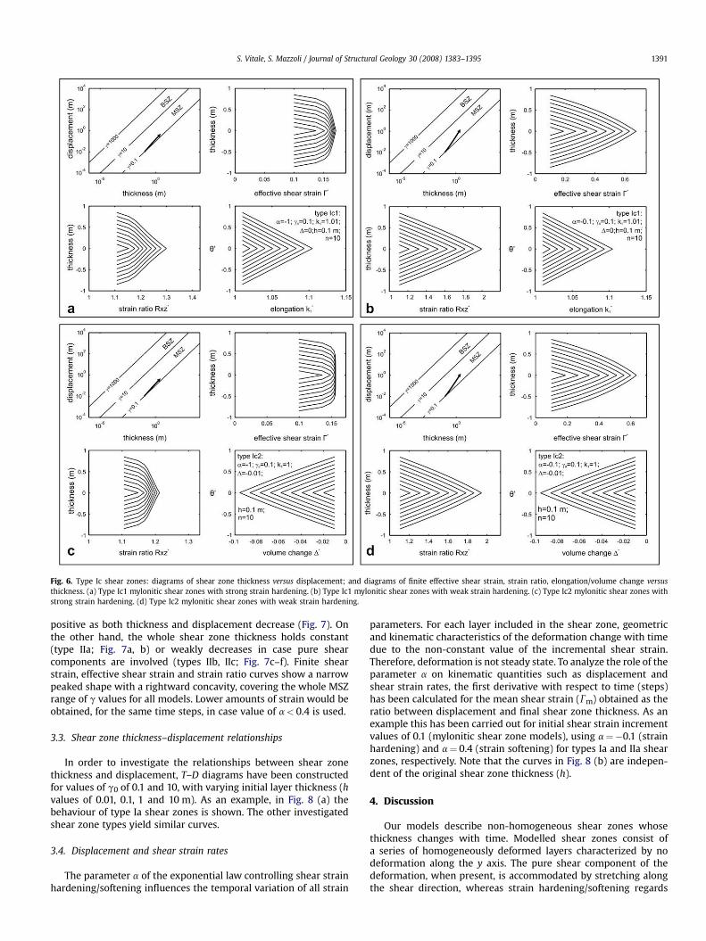
Fig. 6. Type Ic shear zones: diagrams of shear zone thickness versus displacement; and diagrams of finite effective shear strain, strain ratio, elongation/volume change versusthickness. (a) Type Ic1 mylonitic shear zones with strong strain hardening. (b) Type Ic1 mylonitic shear zones with weak strain hardening. (c) Type Ic2 mylonitic shear zones withstrong strain hardening. (d) Type Ic2 mylonitic shear zones with weak strain hardening.


positive as both thickness and displacement decrease (Fig. 7). Onthe other hand, the whole shear zone thickness holds constant(type IIa; Fig. 7a, b) or weakly decreases in case pure shearcomponents are involved (types IIb, IIc; Fig. 7c–f). Finite shearstrain, effective shear strain and strain ratio curves show a narrowpeaked shape with a rightward concavity, covering the whole MSZrange of g values for all models. Lower amounts of strain would beobtained, for the same time steps, in case value of a< 0.4 is used.

3.3. Shear zone thickness–displacement relationships

In order to investigate the relationships between shear zonethickness and displacement, T–D diagrams have been constructedfor values of g0 of 0.1 and 10, with varying initial layer thickness (hvalues of 0.01, 0.1, 1 and 10 m). As an example, in Fig. 8 (a) thebehaviour of type Ia shear zones is shown. The other investigatedshear zone types yield similar curves.

3.4. Displacement and shear strain rates

The parameter a of the exponential law controlling shear strainhardening/softening influences the temporal variation of all strain

parameters. For each layer included in the shear zone, geometricand kinematic characteristics of the deformation change with timedue to the non-constant value of the incremental shear strain.Therefore, deformation is not steady state. To analyze the role of theparameter a on kinematic quantities such as displacement andshear strain rates, the first derivative with respect to time (steps)has been calculated for the mean shear strain (Gm) obtained as theratio between displacement and final shear zone thickness. As anexample this has been carried out for initial shear strain incrementvalues of 0.1 (mylonitic shear zone models), using a¼�0.1 (strainhardening) and a¼ 0.4 (strain softening) for types Ia and IIa shearzones, respectively. Note that the curves in Fig. 8 (b) are indepen-dent of the original shear zone thickness (h).

4. Discussion

Our models describe non-homogeneous shear zones whosethickness changes with time. Modelled shear zones consist ofa series of homogeneously deformed layers characterized by nodeformation along the y axis. The pure shear component of thedeformation, when present, is accommodated by stretching alongthe shear direction, whereas strain hardening/softening regards

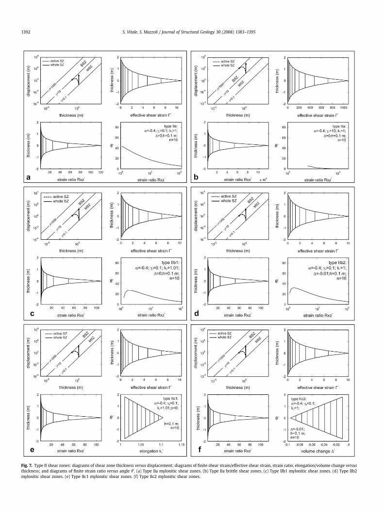
Fig. 7. Type II shear zones: diagrams of shear zone thickness versus displacement; diagrams of finite shear strain/effective shear strain, strain ratio, elongation/volume change versusthickness; and diagrams of finite strain ratio versus angle q’. (a) Type IIa mylonitic shear zones. (b) Type IIa brittle shear zones. (c) Type IIb1 mylonitic shear zones. (d) Type IIb2mylonitic shear zones. (e) Type IIc1 mylonitic shear zones. (f) Type IIc2 mylonitic shear zones.


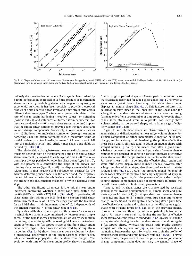
Fig. 8. (a) Diagram of shear zone thickness versus displacement for type Ia mylonitic (MSZ) and brittle (BSZ) shear zones, with initial layer thickness of 0.01, 0.1, 1 and 10 m. (b)Diagrams of time steps versus shear strain rate for type Ia shear zones (with weak strain hardening) and for type IIa shear zones.


uniquely the shear strain component. Each layer is characterized bya finite deformation expressed as a finite product of incrementalstrain matrices. By modelling strain hardening/softening using anexponential function, it has been possible to provide theoreticalprofiles of finite effective shear strain and finite strain ratio acrossdifferent shear zone types. The function exponent a is related to therate of shear strain hardening (negative values) or softening(positive values), and influences all further strain parameters. Forinstance, a value of a¼�0.1 (weak shear strain hardening) impliesthat the simple shear component prevails over the pure shear andvolume change components. Conversely, a lower value (such asa¼�1) disallows the simple shear component (strong shear strainhardening). For the strain softening case, a maximum value ofa¼ 0.4 has been used to allow displacement/thickness curves to fallinto the mylonitic (MSZ) and brittle (BSZ) shear zone fields asdefined by Hull (1988).

The relationship existing between shear zone displacement andthickness depends both on the parameter a and on the initial shearstrain increment g0 imposed to each layer at time t¼ 0. This rela-tionship is always positive for widening shear zones (type I, a< 0),with the parameter a controlling the slope of the curves. Forthinning shear zones (type II, a> 0), the displacement–thicknessrelationship is first negative and subsequently positive for theactively deforming shear zone. On the other hand, the displace-ment–thickness curve for the whole shear zone is either parallel tothe ordinate axis (i.e. constant thickness) or with a negative steepslope.

The other significant parameter is the initial shear strainincrement controlling whether a shear zone plots within theductile (MSZ) or brittle (BSZ) fields (Figs. 4–8). In particular, allshear zones plot within the MSZ field for a chosen initial shearstrain increment value of 0.1, whereas they plot into the BSZ fieldfor an initial shear strain increment value of 10, independently ofthe original thickness (h) of the shear zone (Fig. 8a).

Types Ia and IIa shear zones represent the ‘classical’ shear zonesin which deformation is accommodated by heterogeneous simpleshear. For the type Ia increasing thickness is driven by shear strainhardening, whereas for type IIa decreasing thickness is due to shearstrain softening. The flat-topped shape of the finite shear straincurve across type I shear zones characterized by strong strainhardening (Fig. 4a, b) shows how shear zone evolution involvesa progressive deactivation of the strain-hardened inner sector,while deformation propagates into the shear zone margins. Theevolution with time of the shear strain profile, shows a transition

from an original peaked shape to a flat-topped shape, conforms tothat classically described for type I shear zones (Fig. 1). For type Iashear zones (weak strain hardening), the shear strain curvedisplays an angular shape (Fig. 4c, d). This feature indicates thatdeformation takes place in the inner part of the shear zone fora long time, the shear strain and strain ratio curves becomingflattened only after a large number of time steps. For type IIa shearzones, shear strain and strain ratio profiles consistently showa characteristic, narrow peaked shape, with a large range of ellip-ticity values (Fig. 7a, b).

Types Ib and IIb shear zones are characterized by localizedgeneral shear and distributed pure shear and/or volume change. Fora small component of either incremental elongation or volumechange, and for a strong strain hardening, the profiles of effectiveshear strain and strain ratio tend to attain an angular shape withstraight limbs (Fig. 5a, c). This means that, after a given time,a balance between simple shear and pure shear/volume changecomponents is reached, holding to a constant increase of effectiveshear strain from the margins to the inner sector of the shear zone.For weak shear strain hardening, the effective shear strain andstrain ratio curves display more rounded shapes; however, aftera large number of time steps, also these profiles tend to attainstraight limbs (Fig. 5b, d). As in the previous model, for type IIbshear zones effective shear strain and ellipticity profiles display anangular shape, suggesting that the presence of pure shear and/orvolume change components does not significantly influence theoverall characteristics of finite strain parameters.

Type Ic and IIc shear zones are characterized by localizedgeneral shear involving simultaneous: (i) simple shear and pureshear (types Ic1 and IIc1), (ii) simple shear and volume change(types Ic2 and IIc2), or (iii) simple shear, pure shear and volumechange. In case (i) and for strong strain hardening after a given timethe effective shear strain and strain ratio curves display an angularshape with straight limbs (Fig. 6a), as in the previous model.However, in this case there is strain incompatibility between thelayers. For weak shear strain hardening the profiles of effectiveshear strain and strain ratio are rounded (Fig. 6b). In case (ii) and forstrong strain hardening the effective shear strain curve shows againa flat-topped shape, whereas the strain ratio profile displaysstraight limbs after a given time (Fig. 6c) and strain compatibility ismaintained between the layers. For weak shear strain the profiles ofeffective shear strain and strain ratio are rounded (Fig. 6d). For typeIIc shear zones, the presence of localized pure shear and/or volumechange components again does not vary the general shape of


effective shear strain and ellipticity curves, although incompati-bility between layers, characterized by different finite strain, arises.

Taking into account all possible configurations for the strainhardening models, it is worth noting that the classic flat-toppedshape of the effective shear strain curve, characteristic of type Ishear zones as reported in previous papers, is actually distinctive oftypes Ia and Ic2 only. More frequently, a peaked shape is obtained,whereas for type II shear zones the shear strain and especially theellipticity profiles display always a narrow angular shape withconcavity toward the right. Shear strain rates (Fig. 8b) alwaysincrease with time for type Ia shear zones, tending asymptoticallyto a constant value for a large number of time steps. Conversely, fortype IIa shear zones the curve shows a well-defined maximum andis characterized by higher values with respect to the previousmodel.

In order to compare our modelling results with natural shearzones, some considerations about the possible real values of thetime unit (step) introduced in the models are noteworthy. Forexample, shear strain rates for structures plotting within the MSZfield and characterized by weak shear strain hardening (a¼�0.1)show a mean value of 0.04 step�1, whereas for shear strain soft-ening (a¼ 0.4) a mean value of 0.70 step�1 (Fig. 8b). By comparingthese values with a shear strain of 10�13 s�1 (i.e. within the range oftypical values of natural ductile shear zones; Schmid, 1975; Pfiffnerand Ramsay, 1982; Hacker et al., 1992; Vitale et al., 2007), the timestep of our models may be estimated as of ca. 104–105 years. Relatedmaximum displacement rates attain values of 0.01 and 0.10 mm/year for mylonitic widening and thinning shear zones, respectively.For brittle structures, maximum displacement rates are of 1 mm/yfor widening shear zones, and 10 mm/y for thinning ones.

A few interesting considerations may arise by comparing strainhardening and softening models, as discussed in the followingpoints.

(1) The geometric finite configurations are essentially similar forboth models, being the same for types Ia and IIa (Figs. 2, 3). Inorder to distinguish the driving mechanism (strain hardeningor softening), the shear strain profile across the shear zoneneeds to be analyzed. However, the profiles obtained in casepure shear and volume change components, and/or variableamounts of strain hardening are involved in the deformation,show more complex patterns with respect to the curvesdescribed by Hull (1988). In particular, as peaked-shapedcurves are not restricted to the strain softening case, the simplecriterion of flat-topped versus peaked-shaped curves is notsufficient to distinguish between widening and thinning shearzones.

(2) Both strain hardening and softening models fit the data obtainedfrom natural shear zones, T–D curves falling into the myloniticand brittle fields defined by Hull (1988). However, in order toencompass the whole range of natural shear strains (fromg¼ 0.1 to g¼ 10 for mylonitic shear zones, and from g¼ 10 tog¼ 1000 for brittle ones), strain hardening models must beworking for a long time. The example of Fig. 4 (e, f) shows that,even for a very weak strain hardening (a¼�0.001), a largenumber of steps (n¼ 100, i.e.106–107 years) are needed to obtaincurves extending over the entire MSZ and BSZ fields. On theother hand, strain softening models require a time span of oneorder of magnitude less to achieve comparable finite strains.

(3) Both models allow for a maximum variation of three orders ofmagnitude in size of both thickness and displacement (Figs.4–8). Therefore, based on our results, the question posed byHull (1988) of whether large shear zones can grow fromsmaller ones might be affirmatively answered, although it isenvisaged that the process could occur only within a limitedsize range.

5. Conclusions

Mathematical models may be effectively used to describe thetheoretical behaviour of heterogeneous shear zones characterizedby increasing (type I) or decreasing (type II) thickness with time.Shear zone modelling may be carried out by taking into accountdifferent types and degrees of localization of the deformation,assuming decreasing or increasing shear strain rate due, to shearstrain hardening or softening, respectively. In these conditions, theshear strain must be a monotonic function of time. In this study,a simple exponential function is used to allow for comparison withreal quantities for different shear zone types. With respect toprevious models of type I shear zones, classically characterized bya flat-topped shear strain profile across the shear zone (Hull, 1988),our study indicates that they may also display a peaked-shapedcurve in case pure shear and/or volume change components arepresent. Conversely, type II shear zones are consistently charac-terized by angular shaped profiles with a rightward concavity.

All models depend on a series of parameters such as: (i) theexponent of the shear strain-time function, (ii) the initial shearstrain increment imposed to the system, and (iii) the thickness ofeach homogeneously deformed layer composing the shear zone. Byvarying these parameters it is possible to model weak or strongshear strain hardening/softening, as well as the relationshipbetween displacement (D) and shear zone thickness (T). This allowsfor a quantitative description of brittle and ductile shear zonebehaviours, these being characterized by high and low D/T ratio,respectively.

Comparing mean shear strain rates for type Ia and IIa shearzones with a mean value of 10�13 s�1 (compatible with naturalductile shear zones), our models yield maximum displacementrates of 0.01 (for widening shear zones) and 0.10 (for thinning shearzones) mm/y for mylonitic structures, and of 1 (for widening shearzones) and 10 (for thinning shear zones) mm/y for brittle features,both regardless of shear zone thickness. Our results confirm thattheoretical modelling of heterogeneous shear zone behaviour mayprovide useful insights into the modes of finite strain anddisplacement accumulation in ductile and brittle shear zones.

Acknowledgements

We thank V. Guerriero for helpful discussions and JSG reviewersJ.-L. Bouchez, T. Takeshita, and associate editor J. Hippertt, for theuseful comments that allowed us to significantly improve thepaper.

References

Baird, G.B., Hudleston, P.J., 2007. Modeling the influence of tectonic extrusion andvolume loss on the geometry, displacement, vorticity, and strain compatibilityof ductile shear zones. Journal of Structural Geology 29, 1665–1678.

Fossen, H., Tikoff, B., 1993. The deformation matrix for simultaneous simpleshearing, pure shearing and volume change, and its application to trans-pression–transtension tectonics. Journal of Structural Geology 15, 413–422.

Hacker, B.R., Yin, A., Christie, J.M., Davis, G.A., 1992. Rheology of an extended middlecrust inferred from quartz grain sizes in the Whipple Mountains, California.Tectonics 11, 36–46.

Horsman, E., Tikoff, B., 2007. Constraints on deformation path from finite straingradients. Journal of Structural Geology 29, 256–272.

Hull, J., 1988. Thickness–displacement relationships for deformation zones. Journalof Structural Geology 10, 431–435.

Means, W.D., 1984. Shear zones of types I and II and their significance for recon-struction of rock history. Geological Society of America Abstracts 16, 50.

Means, W.D., 1995. Shear zones and rock history. Tectonophysics 247, 157–160.Pfiffner, O.A., Ramsay, J.G., 1982. Constraints on geological strain rates: arguments

from finite strain states of naturally deformed rocks. Journal of GeophysicalResearch 87, 311–321.

Ramsay, J.G., 1980. Shear zone geometry: a review; shear zones in rocks. Journal ofStructural Geology 2, 83–99.

Ramsay, J.G., Graham, R.H., 1970. Strain variation in shear belts. Canadian Journal ofEarth Sciences 7, 786–813.


Ramsay, J.G., Huber, M., 1987. Folds and Fractures. In: The Techniques of ModernStructural Geology, vol. I. Academic Press, London.

Ring, U., 1998. Volume strain, strain type and flow path in a narrow shear zone. GeolRundsch 86, 786–801.

Schmid, S., 1975. The Glarus overthrust: field evidence and mechanical model.Eclogae Geologicae Helvetiae 68, 247–280.

Srivastava, H.B., Hudleston, P., Earley III, D., 1995. Strain and possible volume loss ina high-grade ductile shear zone. Journal of Structural Geology 17, 1217–1231.

Vitale, S., White, J.C., Iannace, A., Mazzoli, S., 2007. Ductile strain partitioning inmicritic limestones, Calabria, Italy: the roles and mechanisms of intracrystallineand intercrystalline deformation. Canadian Journal of Earth Sciences 44,1587–1602.

heterogeneous shear zone evolution: the role of shear strain hardening/softening

Documents