high doppler resolution imaging by multistatic continuous ... · report documentation page form ......

Calhoun: The NPS Institutional Archive

Theses and Dissertations Thesis Collection

2007-12

High doppler resolution imaging by multistatic

continuous wave radars using constructive techniques

Soh, Wei Ting.

Monterey California. Naval Postgraduate School

http://hdl.handle.net/10945/3148

NAVAL

POSTGRADUATE SCHOOL

MONTEREY, CALIFORNIA

THESIS

Approved for public release; distribution is unlimited

HIGH DOPPLER RESOLUTION IMAGING BY MULTISTATIC CONTINUOUS WAVE RADARS

USING CONSTRUCTIVE TECHNIQUES

by

Wei Ting Soh

December 2007

Thesis Advisor: Brett Borden Second Reader: Donald Walters

THIS PAGE INTENTIONALLY LEFT BLANK

i

REPORT DOCUMENTATION PAGE Form Approved OMB No. 0704-0188 Public reporting burden for this collection of information is estimated to average 1 hour per response, including the time for reviewing instruction, searching existing data sources, gathering and maintaining the data needed, and completing and reviewing the collection of information. Send comments regarding this burden estimate or any other aspect of this collection of information, including suggestions for reducing this burden, to Washington headquarters Services, Directorate for Information Operations and Reports, 1215 Jefferson Davis Highway, Suite 1204, Arlington, VA 22202-4302, and to the Office of Management and Budget, Paperwork Reduction Project (0704-0188) Washington DC 20503. 1. AGENCY USE ONLY (Leave blank)

2. REPORT DATE December 2007

3. REPORT TYPE AND DATES COVERED Master’s Thesis

4. TITLE AND SUBTITLE High Doppler Resolution Imaging by Multistatic Continuous Wave Radars Using Constructive Techniques 6. AUTHOR(S) Wei Ting Soh

5. FUNDING NUMBERS

7. PERFORMING ORGANIZATION NAME(S) AND ADDRESS(ES) Naval Postgraduate School Monterey, CA 93943-5000

8. PERFORMING ORGANIZATION REPORT NUMBER

9. SPONSORING /MONITORING AGENCY NAME(S) AND ADDRESS(ES) N/A

10. SPONSORING/MONITORING AGENCY REPORT NUMBER

11. SUPPLEMENTARY NOTES The views expressed in this thesis are those of the author and do not reflect the official policy or position of the Department of Defense or the U.S. Government. 12a. DISTRIBUTION / AVAILABILITY STATEMENT Approved for public release; distribution in unlimited

12b. DISTRIBUTION CODE

13. ABSTRACT (maximum 200 words) The multistatic radar offers many advantages over monostatic radar in certain applications, especially since the receiving

stations may be located at covert and distant sites relative to the transmitting stations. Furthermore, continuous wave radars are relatively simple and inexpensive to employ and maintain. Hence, the impetus for developing a CW multistatic radar system for high-resolution imaging was conceived.

This thesis is a proof of concept demonstration that a Doppler-only multistatic radar system can be employed to provide high resolution imaging of airborne targets in support of non-cooperative target recognition. Through an understanding of conventional imaging techniques and formulation of the inverse problem in radar imaging, a demonstration radar model based on one transmitter and two receivers was designed to determine the accurate position and velocity of simulated targets. The extraction errors resulted from the range, bearing and velocity measurements were congruent with the physical limitations of each transmitter-receiver pair. Through the employment of a multistatic system, the geometrical diversity allowed these limitations to be overcome.

15. NUMBER OF PAGES

95

14. SUBJECT TERMS High Doppler Resolution, Radar Imaging, Multistatic, Bistatic

16. PRICE CODE

17. SECURITY CLASSIFICATION OF REPORT

Unclassified

18. SECURITY CLASSIFICATION OF THIS PAGE

Unclassified

19. SECURITY CLASSIFICATION OF ABSTRACT

Unclassified

20. LIMITATION OF ABSTRACT

UU NSN 7540-01-280-5500 Standard Form 298 (Rev. 2-89) Prescribed by ANSI Std. 239-18

ii


iii

Approved for public release; distribution is unlimited

HIGH DOPPLER RESOLUTION IMAGING BY MULTISTATIC CONTINUOUS WAVE RADARS

USING CONSTRUCTIVE TECHNIQUES

Wei Ting Soh Major, Republic of Singapore Air Force

Bachelor of Engineering (EEE), Nanyang Technological University, 2001

Submitted in partial fulfillment of the requirements for the degree of

MASTER OF SCIENCE IN COMBAT SYSTEMS SCIENCES AND TECHNOLOGY

from the

NAVAL POSTGRADUATE SCHOOL December 2007

Author: Wei Ting Soh

Approved by: Professor Brett Borden Thesis Advisor

Professor Donald Walters Second Reader

Professor James Luscombe Chairman, Department of Physics

iv


v

ABSTRACT

The multistatic radar offers many advantages over monostatic radar in certain

applications, especially since the receiving stations may be located at covert and distant

sites relative to the transmitting stations. Furthermore, continuous wave radars are

relatively simple and inexpensive to employ and maintain. Hence, the impetus for

developing a CW multistatic radar system for high-resolution imaging was conceived.

This thesis is a proof of concept demonstration that a Doppler-only multistatic

radar system can be employed to provide high resolution imaging of airborne targets in

support of non-cooperative target recognition. Through an understanding of conventional

imaging techniques and formulation of the inverse problem in radar imaging, a

demonstration radar model based on one transmitter and two receivers was designed to

determine the accurate position and velocity of simulated targets. The extraction errors

resulted from the range, bearing and velocity measurements were congruent with the

physical limitations of each transmitter-receiver pair. Through the employment of a

multistatic system, the geometrical diversity allowed these limitations to be overcome.

vi


vii

TABLE OF CONTENTS

I. INTRODUCTION........................................................................................................1 A. DOPPLER-ONLY MULTISTATIC RADAR IMAGING...........................1 B. OBJECTIVE ....................................................................................................2 C. THESIS ORGANIZATION............................................................................2

II. RADAR IMAGING METHODS................................................................................5 A. OVERVIEW OF IMAGING RADAR...........................................................5 B. ONE-DIMENSIONAL IMAGING.................................................................5 C. TWO-DIMENSIONAL IMAGING ...............................................................7 D. HIGH DOPPLER RESOLUTION (HDR) IMAGING ................................9

III. INVERSE PROBLEMS IN RADAR IMAGING....................................................11 A. GENERAL FORMULATION OF THE IMAGING PROBLEM.............11 B. INVERSE PROBLEMS ................................................................................11 C. WELL-POSED AND ILL-POSED PROBLEMS .......................................12 D. METHOD OF LEAST SQUARES...............................................................14 E. CORRELATION RECEPTION...................................................................16 F. AMBIGUITY FUNCTION ...........................................................................18

1. Ambiguity Function for HRR Signal ...............................................18 2. Ambiguity Function for HDR Signal ...............................................19 3. Bistatic Ambiguity Function .............................................................19

IV. BISTATIC AND MULTSTATIC RADAR THEORY ...........................................21 A. BACKGROUND ............................................................................................21 B. DEFINITION OF BISTATIC RADAR .......................................................22 C. COORDINATE SYSTEM.............................................................................22 D. TARGET LOCATION..................................................................................23 E. TARGET DOPPLER ....................................................................................25 F. DOPPLER RESOLUTION...........................................................................26 G. DEFINITION OF MULTISTATIC RADAR..............................................27 H. MAIN ADVANTAGES .................................................................................28

1. Accurate Position Estimate of Targets.............................................29 2. Doppler Estimation of Target Velocity and Acceleration..............29 3. Measurement of Three Dimensional Coordinates and Velocity....29 4. Increased “Signal Information” of Target Body.............................30 5. Increased Resolution..........................................................................30 6. Power Advantages..............................................................................30 7. Configurable Coverage Area ............................................................31 8. Improved Clutter Rejection..............................................................31

I. MAIN DRAWBACKS...................................................................................31 1. Synchronization, Phasing and Transmission of Reference

Signals .................................................................................................32 2. Requirement for Direct Line of Sight between Stations and

Targets ................................................................................................32

viii

3. Need for Data Transmission Lines ...................................................32 4. Increased Processing Requirement ..................................................32 5. Need for Accurate Station Positioning and Mutual Alignment.....33

J. IMPLEMENTATION REQUIREMENTS .................................................33

V. RADAR MODEL DESIGN.......................................................................................35 A. ASSUMPTIONS.............................................................................................35 B. MODEL NOTATIONS .................................................................................36 C. TARGET BEARING AND RANGE RELATIVE TO

TRANSMITTER............................................................................................37 D. TARGET BEARING AND RANGE RELATIVE TO RECEIVERS.......38 E. TARGET VELOCITY VECTOR ................................................................40

VI. RADAR MODEL IMPLEMENTATION AND RESULTS...................................43 A. SCENARIO SETUP.......................................................................................43 B. TEST DATA GENERATION.......................................................................44

1. Data Available to Radar System.......................................................44 2. Data for Results Comparison and Analysis.....................................44

C. LEAST SQUARES IMPLEMENTATION .................................................46 D. EXTRACTION OF TARGET POSITION INFORMATION...................47

1. Transmitter to Receiver “Round-trip” Distance ............................48 2. Target Bearing and Range Relative to Receivers (R1 & R2).........48

E. EXTRACTION OF TARGET VELOCITY INFORMATION.................50

VII. ERROR ANALYSIS..................................................................................................53 A. OVERVIEW...................................................................................................53 B. ERRORS IN BEARING MEASUREMENT...............................................53 C. ERRORS IN VELOCITY MEASUREMENT ............................................56 D. ERRORS WITH ADDITIVE GAUSSIAN NOISE ....................................58

VIII. RECOMMENDATIONS AND CONCLUSION.....................................................67 A. RECOMMENDATIONS FOR FUTURE WORK......................................67

1. More Complex Scenarios ..................................................................67 2. Performance in Real World Environment ......................................67 3. Analysis of Bistatic Ambiguity Function .........................................68

B. CONCLUSION ..............................................................................................68

APPENDIX.............................................................................................................................69

LIST OF REFERENCES......................................................................................................77

INITIAL DISTRIBUTION LIST .........................................................................................79

ix

LIST OF FIGURES

Figure 1. Example of a range profile of a Boeing 737-500 (From [5]).............................6 Figure 2. Ambiguity scenario from a single pulse ............................................................7 Figure 3. Cross-range information obtained from range profiles......................................8 Figure 4. Orthogonal “slices” of the target between using HRR and HDR (After [2]) ....9 Figure 5. Image formation model....................................................................................11 Figure 6. Bistatic radar ....................................................................................................22 Figure 7. Bistatic radar (North referenced) coordinate system .......................................23 Figure 8. Bistatic Doppler geometry ...............................................................................25 Figure 9. Bistatic Doppler resolution (for 2 collocated targets)......................................27 Figure 10. Sample Multistatic radar configuration (1 transmitter & 2 receivers) .............28 Figure 11. Framework for initial Multistatic radar model.................................................35 Figure 12. Bistatic triangle involving T1, R1 and TGT ....................................................38 Figure 13. Plan view schematic of scenario setup.............................................................43 Figure 14. Radar positions and target flight paths.............................................................46 Figure 15. Plot of Tgt #1 and Tgt #2 from measured data in Receiver R1 .......................49 Figure 16. Plot of Tgt #1 and Tgt #2 from measured data in Receiver R2 .......................49 Figure 17. Velocity magnitude of Tgt #1 and Tgt #2 from measured data.......................51 Figure 18. Velocity direction of Tgt #1 and Tgt #2 from measured data..........................51 Figure 19. Bearing error for Tgt #2 as seen from receiver R1 ..........................................54 Figure 20. Extended baseline of Transmitter-Receiver pair for T1-R1 ............................54 Figure 21. Bearing error for Tgt #1 as seen from receiver R2 ..........................................55 Figure 22. Extended baseline of Transmitter-Receiver pair for T1-R2 ............................56 Figure 23. Velocity magnitude error for Tgt #1................................................................57 Figure 24. Velocity magnitude error for Tgt #2................................................................57 Figure 25. Erroneous regions for velocity magnitude measurements ...............................58 Figure 26. Range error for Tgt #1 as seen from receiver R1 (with 2% Gaussian noise) ..59 Figure 27. Bearing error for Tgt #1 as seen from receiver R1 (with 2% Gaussian

noise)................................................................................................................59 Figure 28. Velocity magnitude error for Tgt #1 (with 2% Gaussian noise)......................60 Figure 29. Velocity direction error for Tgt #1 (with 2% Gaussian noise) ........................60 Figure 30. Range error for Tgt #1 as seen from receiver R1 (with 10% Gaussian

noise)................................................................................................................61 Figure 31. Bearing error for Tgt #1 as seen from receiver R1 (with 10% Gaussian

noise)................................................................................................................62 Figure 32. Standard deviation in range errors for various amounts of Gaussian noise.....63 Figure 33. Standard deviation in bearing errors for various amounts of Gaussian noise..64 Figure 34. Standard deviation in velocity magnitude errors for various amounts of

Gaussian noise .................................................................................................64 Figure 35. Standard deviation in velocity direction errors for various amounts of

Gaussian noise .................................................................................................65

x


xi

LIST OF TABLES

Table 1. Properties of bistatic Doppler shift under various conditions (From [22])......26 Table 2. Notations used in multistatic radar model .......................................................36 Table 3. Radar stations and targets’ disposition and other parameters..........................44 Table 4. Data for results comparison and analysis.........................................................45 Table 5. Average error and standard deviation in target position errors........................50 Table 6. Average error and standard deviation in target velocity errors........................52 Table 7. Standard deviation of the different types of errors for various amounts of

Gaussian Noise.................................................................................................62

xii


xiii

ACKNOWLEDGMENTS

I would like to express my deep and sincere gratitude to my thesis advisor,

Professor Brett Borden. His understanding, encouragement and personal guidance

provided a good basis for this thesis. His critical ideas and patience in working with me

on an outline made the forging of this thesis possible. His extensive knowledge and

logical way of thinking have been of great value to me, especially during those periods

when I seemed to have reached a dead-end in my research. This work would not have

been possible if not for his professional and personal attention.

I also wish to express my warm and sincere thanks to my thesis co-advisor,

Professor Donald Walters. His recommendations have been very welcoming and quite

insightful to my understanding of the research topics.

I especially want to thank my colleague and friend in the inverse scattering

laboratory, LT Armando Lucrecio. His kind assistance and tips on the use of Apple

computers facilitated my smooth initiation into the laboratory. His knowledge in radar

imaging and digital signal processing provided valuable insights into my research. His

friendship and encouragement motivated me to persevere in times of difficulty.

Finally, I want to give special thanks to my lovely wife, Sheau Shyuan. It has

been a difficult year for her, especially since she has to look after our newborn daughter

Yenn Shan, in Singapore while I endeavored to complete my research in Monterey.

Without her understanding and support, it would have been impossible for me to finish

this work.

xiv


1

I. INTRODUCTION

A. DOPPLER-ONLY MULTISTATIC RADAR IMAGING

IEEE Standard 686-1997 [1] defined the multistatic radar as a radar system

having two or more transmitting or receiving antennas with all antennas separated by

large distances when compared to the antenna sizes. It has at least three components —

for instance, one transmitter and two receivers, or multiple receivers and multiple

transmitters. It is a generalization of the bistatic radar system, with one or more receivers

processing echo field returns from one or more geographically separated transmitters.

The multistatic radar system is desirable as it allows covert operation of the receivers and

there is increased resilience to electronic countermeasures. Additionally, due to

geometrical effects, the radar cross-section of the target could potentially be enhanced.

Conventional synthetic aperture radar or inverse synthetic aperture radar imaging

involves the processing of short pulse signals to form high range resolution images of the

target. Similarly, high Doppler resolution data could be utilized to generate images. One

major benefit of employing high Doppler resolution imaging in a multistatic radar system

is the requirement for relatively simple and inexpensive continuous wave (CW)

transmitters and receivers. For a typical airborne target, the signal returns are

intrinsically considered narrowband since the Doppler shifts are usually in the region of

tens to hundreds of kilohertz. This narrowband attribute in a Doppler imaging system has

utility in operations where the available frequency spectrum is limited.

Conceptually, a Doppler-only multistatic radar system could potentially provide

high-resolution imaging of airborne targets in support of non-cooperative target

recognition [2], while keeping the cost and ease of implementation and maintenance to a

significantly lower level when compared with current pulse-Doppler monostatic radars.

This is the subject of this thesis.

2

B. OBJECTIVE

The objective of this thesis is to develop a basic theory for a Doppler-only

multistatic radar system based on high-Doppler resolution data. The physics involved in

resolving the geometry of the targets relative to the transmitters and receivers, as well as

the imaging process will be discussed. The mathematical implementation of such a radar

system will also be examined. Thereafter, the results of the above analysis will be

exercised on test cases.

C. THESIS ORGANIZATION

The thesis is divided into eight chapters, organized as follows.

Chapter II provides a review of current imaging methods, including one-

dimensional high range resolution imaging, its extension to two-dimensional imaging,

and high Doppler resolution imaging.

Chapter III provides some background of inverse problems in radar imaging. The

well-posedness and condition number of the problem, and the method of least squares are

discussed.

Chapter IV introduces the concepts of bistatic radars. It presents an overview of

bistatic radar definitions and the parameters involved in the derivation of the model.

Thereafter, it extends the bistatic model into the multistatic case. The advantages and

disadvantages of the multistatic radar, as well as the implementation requirements, are

discussed.

Chapter V introduces the design of the radar model. It describes the mathematical

approach to derive the target’s position and velocity.

Chapter VI involves the implementation of the multistatic radar model for

imaging. It illustrates the results and tabulation of measurement errors.

3

Chapter VII provides the results analysis and an examination of the imaging

artifacts.

Finally, Chapter VIII recommends areas of future work and concludes with some

comments on the impetus towards developing a Doppler-only multistatic radar system.

4


5

II. RADAR IMAGING METHODS

A. OVERVIEW OF IMAGING RADAR

Radar systems measure the strength of the backscatter and the round trip delay

time of radio frequency signals reflected from distant objects. Since the radar pulse

travels at the speed of light, it is relatively straightforward to use the measured time delay

for the round trip of a particular pulse to calculate the range to the reflecting object. The

resolution in the down-range direction is governed by the pulse bandwidth: a higher

bandwidth will imply finer resolution in this direction. The resolution of the image in the

cross-range direction is determined by the dimensions of the radar antenna and a larger

antenna will lead to finer resolution in the azimuth direction.

This chapter discusses the current imaging methods such as one-dimensional high

range resolution (HRR) imaging, two-dimensional imaging and high Doppler resolution

(HDR) imaging will be discussed.

B. ONE-DIMENSIONAL IMAGING

One-dimensional imaging involves the generation of range profiles, which is a

straightforward method of articulating target substructure. High range resolution imaging

involves the resolution of the individual target scatterers through the down-range profile

of the target. This method essentially provides a one-dimensional image of the target and

an example is shown in Figure 1. Short pulse or pulse-compressed signals can be used to

form one-dimensional HRR images of the target. As the short pulse sweeps across the

target, it sequentially excites the scatterers on the target, which re-radiate energy back to

the radar receiver. When these scatterers are non-interacting and point-like, the scattered

pulse will be a sum of damped and blurred images of the incident pulse, which are shifted

by time delays that are proportional to the scatterer’s range [3]. For pulse compression,

the two common waveforms are linear frequency modulation and binary phase coded

pulses [4].

6

Figure 1. Example of a range profile of a Boeing 737-500 (From [5])

The down-range profile can be affected by a variety of factors such as target

aspect angle, position of the scatterers or masking of scatterers by other parts of the

target. Additionally, since the bandwidth of a pulse is inversely proportional to its

duration, the use of short pulses will lead to large bandwidth requirements. Wide

bandwidth can increase system complexity and increase the likelihood of interference

from other emitters in the electromagnetic spectrum. A short-pulse waveform also

provides less accurate radial velocity measurement as compared to that obtained from

Doppler frequency shift. As high peak power is required to transmit short pulses over

long ranges, it is an important limitation in radar applications. High peak power

transmission can result in voltage breakdown, especially at high frequencies since the

waveguide dimensions are small.

Radar imaging through using only range profiles has limited applications. This is

due to the fact a range profile will not be able to distinguish cross-range target structures.

All scatterers located at the same distance from the radar will reflect energy back to the

radar with the same time delay. Hence, when the radar illuminates many distinct targets

7

at any instant, conclusive decisions pertaining to the nature of the target cannot be

formed using a single set of range-only data [6].

C. TWO-DIMENSIONAL IMAGING

For sufficient target interpretation, other information is usually needed in addition

to the range profile. Such added information can be in the form of a high-resolution

cross-range profile, Doppler profile, or the “triangulation” of range profiles. The

Synthetic Aperture Radar (SAR) and Inverse Synthetic Aperture Radar (ISAR) are

examples of two different schemes of imaging systems that form two-dimensional images

of a target.

“Triangulation” of different sets of range profiles allows the extension of the radar

imaging concept to two dimensions. This approach permits the determination of cross-

range target structure while using only HRR radar systems. It relies on collecting

multiple sets of range profiles from different target orientations, processing them, and

synthesizing an image.

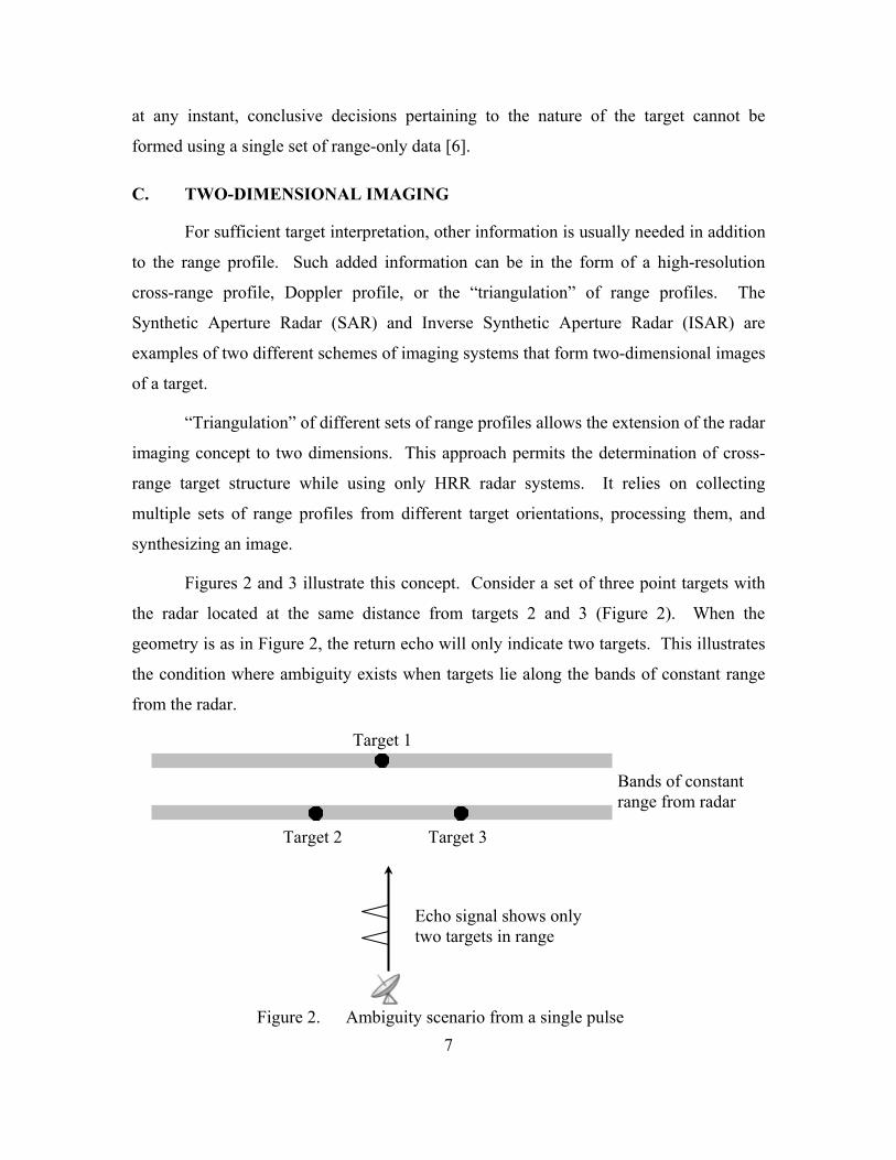
Figures 2 and 3 illustrate this concept. Consider a set of three point targets with

the radar located at the same distance from targets 2 and 3 (Figure 2). When the

geometry is as in Figure 2, the return echo will only indicate two targets. This illustrates

the condition where ambiguity exists when targets lie along the bands of constant range

from the radar.

Figure 2. Ambiguity scenario from a single pulse

Target 1

Target 2 Target 3

Bands of constant range from radar

Echo signal shows only two targets in range

8

With multiple sets of data from different directions, triangulation will allow for

gradual buildup of the relative positions of the three targets (Figure 3). The range

profiles are swept in the cross-range direction to form bands of constant range from the

radar, which represent the possible locations of the target scatterer. These bands are then

superimposed and the crossing points are used to determine the scattering center

locations. With correct correlation methods, a target image built up of points where the

swept lines intersect can be obtained.

Figure 3. Cross-range information obtained from range profiles

In essence, two different schemes are used to collect target data from different

target aspects to obtain cross-range information. The radar can move around the target

while it remains fixed; or the target can rotate while the radar stares at it over time. In the

former case, the radar is described as collecting data over a synthetic aperture, and thus,

termed Synthetic Aperture Radar (SAR). In the latter case, the radar is described as an

Inverse Synthetic Aperture Radar (ISAR). Mathematically, the basics for image

formation are fundamentally the same for both schemes. Notwithstanding, the details of

data processing, such as correcting for departures from ideal target behavior, are different

in the two settings.

Target 1

Target 2 Target 3

9

D. HIGH DOPPLER RESOLUTION (HDR) IMAGING

The concept of utilizing high Doppler resolution inputs to synthesize a target

image can be illustrated by drawing an analogy from HRR imaging.

In HRR imaging, the image is developed by a correlation of range profiles taken

at different locations. Each “line” of the range profile is an iso-range line at a specific

time since the radar pulse takes a finite amount of time to reflect off a scatterer and return

to the receiver.

In HDR, another set of “lines,” the iso-Doppler, which are lines of constant

Doppler shift at a specific frequency, is used to build the image. For a target rotating

about its center, the local velocity of a scatterer will depend on its radial distance from

the center. The return signal at a given Doppler shift is a superposition of all the returns

due to scatterers with the same closing velocity lying along the iso-Doppler hyperbola.

Conceptually, the iso-range lines and iso-Doppler lines can be considered as taking

“slices” of the image, with the difference between the two being the “slices” are

orthogonal to each other, as illustrated in Figure 4 [2].

Figure 4. Orthogonal “slices” of the target between using HRR and HDR (After [2])

HRR down-range “slices” at time intervals

HDR cross-range “slices” at frequency intervals

10

Similarly, ambiguities due to multiple scatterers along an iso-Doppler can be

resolved by acquiring multiple Doppler profiles from different aspect angles. However, it

should be noted that the HDR cross-range slices only works for rotating targets.

In HRR imaging, each range profile has high resolution in the down-range

direction and the correlation of the profiles for different aspect angles will provide the

cross-range resolution to build a two-dimensional image. Conversely, in HDR imaging,

each Doppler profile will have high resolution in the cross-range direction and the

correlation process will provide the down-range resolution.

11

III. INVERSE PROBLEMS IN RADAR IMAGING

A. GENERAL FORMULATION OF THE IMAGING PROBLEM

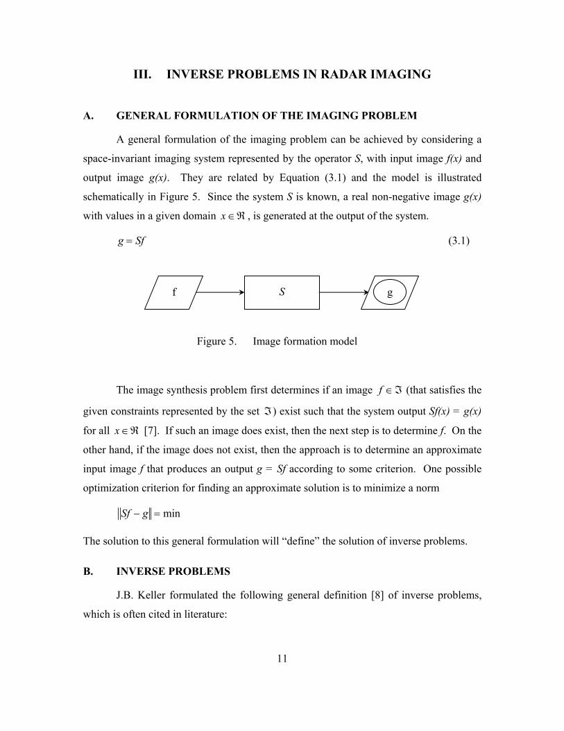
A general formulation of the imaging problem can be achieved by considering a

space-invariant imaging system represented by the operator S, with input image f(x) and

output image g(x). They are related by Equation (3.1) and the model is illustrated

schematically in Figure 5. Since the system S is known, a real non-negative image g(x)

with values in a given domain x ∈ℜ , is generated at the output of the system.

g = Sf (3.1)

Figure 5. Image formation model

The image synthesis problem first determines if an image f ∈ℑ (that satisfies the

given constraints represented by the set ℑ) exist such that the system output Sf(x) = g(x)

for all x ∈ℜ [7]. If such an image does exist, then the next step is to determine f. On the

other hand, if the image does not exist, then the approach is to determine an approximate

input image f that produces an output g = Sf according to some criterion. One possible

optimization criterion for finding an approximate solution is to minimize a norm

Sf − g = min

The solution to this general formulation will “define” the solution of inverse problems.

B. INVERSE PROBLEMS

J.B. Keller formulated the following general definition [8] of inverse problems,

which is often cited in literature:

S f g

12

We call two problems inverses of one another if the formulation of each involves all or part of the solution of the other. Often, for historical reasons, one of the two problems has been studied extensively for some time, while the other is newer and not so well understood. In such cases, the former problem is called the direct problem, while the latter is called the inverse problem.

A direct problem can be thought of as one oriented towards a cause and effect

sequence, while the corresponding inverse problem is linked to the reversal of this cause

and effect sequence and comprises determining the unknown causes of known

consequences. In radar imaging, the direct problem is the mapping from the target to the

quantities that can be measured by the radar.

Consequently, the inverse problem is the problem of finding the original target

given the data and knowledge of the direct problem. This mapping is called the target

image. However, this problem is ill-posed due to the loss of information intrinsic to the

solution of the direct problem. Therefore, if an image corresponds to two distinct objects,

then the solution of the inverse problem is not unique. Further, if there are two

neighboring images such that the corresponding objects are very distant, then the solution

of the inverse problem does not depend continuously on the data.

The accepted approach for solving inverse problems which are ill-posed is to

search for approximate solutions satisfying additional constraints based on the physics of

the problem [12]. This set of approximate solutions corresponding to the same data

function is the set of objects with images close to the measured one.

C. WELL-POSED AND ILL-POSED PROBLEMS

The mathematical term for well-posed problems arose from a classical concept

defined by Hadamard. He believed that such problems are considered well-posed if they

satisfy the following three conditions [10]:

1. the solution is unique

2. the solution exists for any data

3. the solution depends continuously on the data and parameters

13

If one of the three conditions above is not satisfied, the problem is said to be ill-

posed. Hence, an ill-posed problem is one whose solution is not unique and/or does not

exist for any data and/or does not depend continuously on the data.

The third condition is motivated by the fact that the mere process of measuring

data involves small errors. If the problem is well-posed, the error propagation is

controlled by the condition number. Consider the solution of a linear system of algebraic

equations

Ax = m (3.2)

where m is the measured data, x is the signal and A is an operator that describes the

nature of the measurement system. In the case of a unique solution, if there are n

variables, then there must be n independent equations in order to obtain a solution. By

conditions 1 and 2, the inverse of A exists. By thinking of ∆m as being the small error in

the measured data and ∆x as being the resulting error in x such that

A(x + ∆x) = m + ∆m

Consequently, this uncertainty ∆x complies with

∆xx

≤ cond(A)∆mm

where ∆m / m is the relative change in measurement and ∆x / x is the relative

error caused by this change [11].

The condition number is a relative error magnification factor and the quantity that

controls error propagation from data to solution. It is defined as

cond(A) = A A−1

where the common norm of Euclidean distance is adopted for A such that

A = aij

2

j=1

n

∑i=1

m

∑

12

14

It should be noted that the computation of the matrix norm corresponding to the l2-norm

criterion involves the singular value decomposition (SVD). If the condition number of A

is not large, then the problem is considered to be well-conditioned. The solution to the

problem will be stable relative to small variations of data. This requirement of stability is

essential for meaningful problems in approximation methods. On the other hand, if the

condition number is large, then the problem is deemed ill-conditioned. The ill-

conditioned situation is somewhat similar to the ill-posed condition. An ill-posed

problem can be thought of as one where an inverse does not exist because m + ∆m is

outside the range of A.

In general, most inverse problems are ill-posed. In the case of a bandlimited

system, the solution of the inverse problem is not unique and the first condition required

for well-posedness is not satisfied. This is because the imaging system does not transmit

information about the target at frequencies outside the band of the instrument.

Straightforward solutions of ill-posed problems can result in non-physical

answers. It is interesting to note that a more refined operator A may work against

obtaining a more reliable solution. When discretizing an ill-posed problem, the condition

number of the corresponding discrete problem can be very large. It is the case that, when

the discretization of the ill-posed problem gets finer, the condition number of the

corresponding discrete problem becomes larger [9]. For this reason, the discretization of

equations must be done carefully and techniques must be introduced to construct stable

solutions.

D. METHOD OF LEAST SQUARES

An overdetermined system is one that comprises more equations than unknowns.

Overdetermined systems of simultaneous linear equations are often encountered in

various kinds of curve fitting to experimental data. The method of least squares is

frequently used to solve such systems of equations in an approximate sense. During the

process of measuring data, errors or inaccuracies will be manifested in the measurement.

Hence, instead of solving the equations accurately, the minimization of the sum of

15

squares of the residuals is sought. The result is a curve fit to a set of data points such that

the sum of squares of the range between the data point and its corresponding curve is

minimized.

If appropriate probabilistic assumptions about underlying error distributions are

made, the least squares approach becomes what is known as the maximum-likelihood

estimate of the parameters. This least squares criterion (l2 -norm criterion) is widely used

for the resolution of inverse problems due to its simplicity. It should be noted that at

times, it is applied even if its basic underlying hypothesis (Gaussian uncertainties) is not

always satisfied [13].

In the curve fitting model, let t be the independent variable and let m(t) denote the

unknown function of t to be approximated. If there are k observations, then the values of

m measured at specified points of t are

mi = m(ti ), i = 1,2,...,k

The function m(t) is then modeled by a linear combination of n basis functions

m(t) ≈ x1φ1(t) + ....+ xnφn (t)

The design matrix A is a rectangular matrix of order k by n with elements

aij = φ j (ti )

In matrix-vector notation, the model is

m ≈ Ax

There are many models available for the curve fitting solution. Some common models

include the straight line, polynomials, rational functions, exponentials, log-linear and

Gaussian. This thesis will focus on applying the polynomial model for the least squares

application. The model used is a cubic polynomial of the form

m(t) ≈ x1 + x2t + x3t2 + x4t

3

The residuals are the differences between the measurements and the model:

16

ri = mi − x jj=1

n

∑ φ j (ti ) i = 1,2,..., k

= mi − m(t)

= mi − x1 + x2t + x3t2 + x4t

3( )

By the method of least squares, the objective is to minimize the sum of squares of the

residuals:

r 2 = ri2

i=1

k

∑

⇒ r 2 = mi − x1 + x2t + x3t2 + x4t

3( ) 2

i=1

k

∑ (3.3)

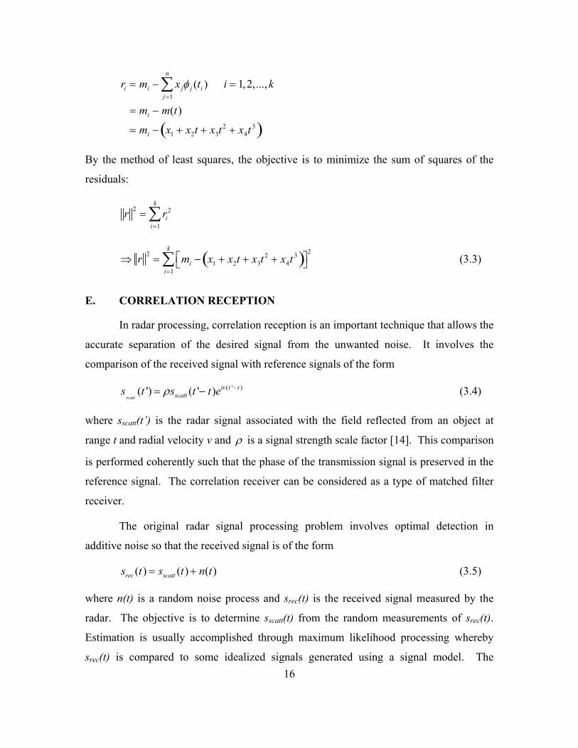
E. CORRELATION RECEPTION

In radar processing, correlation reception is an important technique that allows the

accurate separation of the desired signal from the unwanted noise. It involves the

comparison of the received signal with reference signals of the form

sscatt

(t ') = ρsscatt (t '− t)eiv(t '− t ) (3.4)

where sscatt(t’) is the radar signal associated with the field reflected from an object at

range t and radial velocity v and ρ is a signal strength scale factor [14]. This comparison

is performed coherently such that the phase of the transmission signal is preserved in the

reference signal. The correlation receiver can be considered as a type of matched filter

receiver.

The original radar signal processing problem involves optimal detection in

additive noise so that the received signal is of the form

srec (t) = sscatt (t)+ n(t) (3.5)

where n(t) is a random noise process and srec(t) is the received signal measured by the

radar. The objective is to determine sscatt(t) from the random measurements of srec(t).

Estimation is usually accomplished through maximum likelihood processing whereby

srec(t) is compared to some idealized signals generated using a signal model. The

17

maximum likelihood estimate for sscatt(t) is one which maximizes the probability psr ssc,

which is the conditional probability density function of the measured signal for a specific

scattered field sscatt(t) [6].

sscatt ,ML = arg maxu∈ model space

psr ssc(u)

Consequently, it can be shown that correlation receivers attempt to determine the time

shift, τ , and frequency shift, υ , which maximizes the real part of the correlation integral

η(υ,τ ) = srec (t ')sinc* (t '− τ )e− iυ (t '−τ )dt '

−∞

∞

∫ (3.6)

In radar operations, the natural model is based on the scattering interaction

between the interrogating field and target. If sinc(t) is the incident pulse transmitted by

the radar, then the linear radar scattering model is derived from the superposition of

Equation (3.4).

sscatt (t) = ρ(υ,τ )sinc (t − τ )eiυ (t −τ )dτd−∞

∞

∫∫ υ (3.7)

Now, this model is substituted into Equation (3.5) and then into the correlation integral of

Equation (3.6).

η(υ,τ ) = ρ(υ ',τ ')sinc (t '− τ )sinc* (t '− τ ')eiυ '(t '−τ )e− iυ (t '−τ ')dt 'dτ 'd

−∞

∞

∫∫ υ '∫

+ correlation noise term (3.8)

The correlation noise term is considered small and can thus be ignored. Thereafter,

Equation (3.8) can be rearranged to

η(υ,τ ) = ρ(υ ',τ ')χ(υ −υ ',τ − τ ')ei12

(υ+υ ')(τ −τ ')dτ 'd

−∞

∞

∫∫ υ ' (3.9)

where

χ(υ,τ ) = sinc (t '−12τ )

−∞

∞

∫ sinc* (t '+

12τ )eiυt 'dt ' (3.10)

18

Equation (3.9) is the standard radar data model and expresses the output of the correlation

receiver as the convolution of ρ and χ . The function χ(υ,τ ) defined by Equation (3.10)

is the ambiguity function.

F. AMBIGUITY FUNCTION

The accuracy with which the target position and radial velocity can be estimated

from the radar data is determined by the ambiguity function. In radar systems,

waveforms are selected to optimize the requirements of detection, measurement accuracy,

resolution, and ambiguity and clutter rejection. Ambiguity function plots are scrutinized

for a qualitative determination of the suitability of different waveforms in meeting the

above requirements [4]. In practice, the ambiguity function is plotted as a function of

time delay and Doppler shift. In radar imaging, the ambiguity function can be thought of

as the imaging kernel.

1. Ambiguity Function for HRR Signal

In HRR imaging, the system can be represented by an impulse radar transmitting

a very short pulse in the form of a Dirac delta function

sinc(t) = δ (t)

The ambiguity function becomes

χ(υ,τ ) = sinc (t '−

12τ )

−∞

∞

∫ sinc* (t '+

12τ )eiυt 'dt '

= δ (t '−τ2

)δ (t '+τ2

)−∞

∞

∫ eiυt 'dt '

∴χ(υ,τ ) = δ (τ )eiυ τ

2

The data collected from such a radar is independent of frequency shift and is

known as the down-range profile. In reality, a Dirac delta function does not exist

physically, hence, the waveform used is usually an approximation of an impulse.

19

2. Ambiguity Function for HDR Signal

In HDR imaging, the system can be represented by a continuous wave radar

transmitting a single tone signal in the form

sinc (t) = e− iω t

The ambiguity function then becomes

χ(υ,τ ) = sinc (t '−12τ )

−∞

∞

∫ sinc* (t '+

12τ )eiυt 'dt '

= e− iω (t '−

τ2

)

−∞

∞

∫ eiω (t '+

τ2

)eiυt 'dt '

= eiωτ eiυt '

−∞

∞

∫ dt '

∴χ(υ,τ ) = δ (υ)eiωτ (3.11)

It can be concluded that the data collected is independent of down-range delay.

Consequently, such radar data can be used to determine the distribution of down-range

velocity accurately, but will offer no information about target position.

3. Bistatic Ambiguity Function

For a monostatic radar, the use of delay and Doppler shift as the arguments of the

ambiguity function is sufficient due to the linear relationship between target range and

range rate. Thus, the delay and Doppler shift pair, or the range and range rate pair, may

be used interchangeably in the ambiguity function.

In the case of a bistatic or multistatic radar, the situation is more complicated.

Since the transmitter and receiver are not at the same site, the relationship between

Doppler shift and target velocity, and between time delay and range, are highly non-

linear. The shape of the ambiguity function is a strong function of the geometry between

the transmitter, receiver and target, as well as waveform properties [15]. Hence, the

representation of the ambiguity function for a bistatic radar in terms of delay and Doppler

shift is not meaningful and may even lead to incorrect conclusions.

20

It has been proposed that the ambiguity function for bistatic radar be written as:

χ(RRH , RRa ,VH ,Va ,θR , L) =

s(t − τ a (RRa ,θR , L) ⋅ s*(t − τ H (RRH ,θR , L) ⋅ e − i ωDH (RRH ,VH ,θR ,L )−ωDa (RRa ,Va ,θR ,L )( )t dt−∞

∞

∫2 (3.12)

where RRH and RRa are the hypothesized and actual ranges from the receiver to the target;

VH and Va are the hypothesized and actual radial velocities of the target relative to the

receiver; ωDH and ωDa are the hypothesized and actual Doppler shift; θR is the bearing

of the target with respect to the receiver; and L is the baseline length between the

transmitter and receiver [16]. Equation (3.12) assumes the reference point of the bistatic

geometry to be the receiver. The main difference between Equations (3.12) and (3.10) is

that the geometrical disposition of the transmitter, receiver, and target are taken into

account.

21

IV. BISTATIC AND MULTSTATIC RADAR THEORY

A. BACKGROUND

In monostatic radar systems, increased information is frequently associated with

increased bandwidth. With the increased bandwidth, high range resolution is obtainable

and frequency diversity offers one such approach to obtain additional information about

targets. On the other hand, in a multistatic radar system, geometric diversity [17] in the

disposition of transmitting and receiving stations allows additional target information to

be obtained. With suitable signal processing, the additional information obtained can

translate into improved target detection. Additionally, geometric diversity offers the

potential for increased resolution and it is a dual to frequency diversity in classical

monostatic radar systems. Hence, improved target position accuracy and image

resolution can be expected in a multistatic radar system.

The image resolution for the monostatic synthetic aperture radar (SAR) can be

drawn from tomography/Fourier space or radar range/Doppler principles. In the case of

multistatic SAR, the resolution result is understood using the tomography/Fourier space

principles. As an example, an ultra wideband monostatic SAR with a 50% bandwidth

will have a range resolution of λ and a pixel area of λ2 . A Multistatic SAR system will

have a range resolution of λ / 3 and a pixel area of λ2 / 9 [18]. This translates to a 9.5

dB improvement over monostatic. A similar performance gain can be expected from a

multistatic ISAR system.

Since the bistatic radar is the building block for the multistatic radar system, the

fundamental theory for bistatic radar operation will first be discussed. These will include

the coordinate system, the determination of target location and Doppler information and

resolution. Thereafter, the extension of the bistatic radar to the multistatic radar system,

its advantages and drawbacks, and implementation requirements will be examined.

22

B. DEFINITION OF BISTATIC RADAR

As defined by the IEEE Standard 686-1997 [1], the bistatic radar is a radar using

antennas for transmission and reception at sufficiently different locations that the angles

or ranges from those locations to the target are significantly different. Bistatic radar is

deemed to have significant advantages against stealthy targets due to the relatively larger

amount of forward scattering. Furthermore, the operation of the bistatic radar receiver is

considered covert, as its location cannot be determined easily by merely observing the

radar’s emissions.

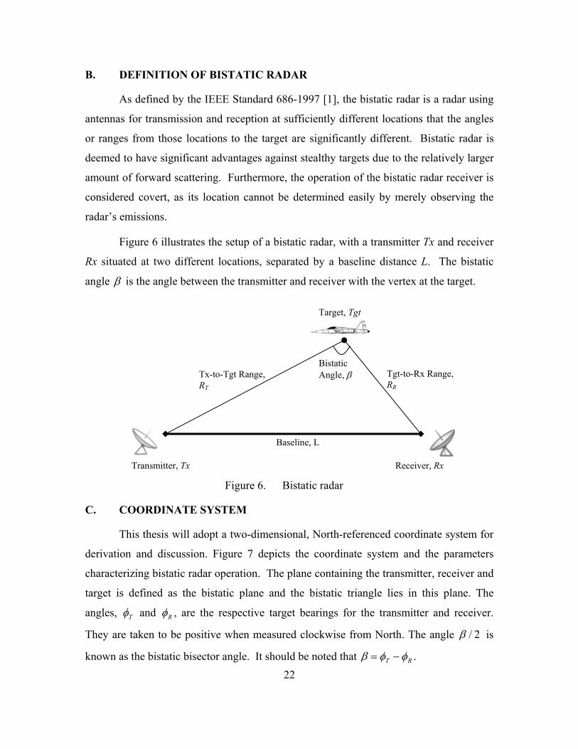
Figure 6 illustrates the setup of a bistatic radar, with a transmitter Tx and receiver

Rx situated at two different locations, separated by a baseline distance L. The bistatic

angle β is the angle between the transmitter and receiver with the vertex at the target.

Figure 6. Bistatic radar

C. COORDINATE SYSTEM

This thesis will adopt a two-dimensional, North-referenced coordinate system for

derivation and discussion. Figure 7 depicts the coordinate system and the parameters

characterizing bistatic radar operation. The plane containing the transmitter, receiver and

target is defined as the bistatic plane and the bistatic triangle lies in this plane. The

angles, φT and φR , are the respective target bearings for the transmitter and receiver.

They are taken to be positive when measured clockwise from North. The angle β / 2 is

known as the bistatic bisector angle. It should be noted that β = φT −φR .

Transmitter, Tx Receiver, Rx

Bistatic Angle, β

Target, Tgt

Baseline, L

Tx-to-Tgt Range, RT

Tgt-to-Rx Range, RR

23

Figure 7. Bistatic radar (North referenced) coordinate system

D. TARGET LOCATION

The target’s position relative to the receiving station can be determined if RR and

φR can be obtained. However, the receiver-to-target range, RR, cannot be measured

directly as a bistatic radar usually measures target range as the range sum RT + RR. It can

be calculated by solving the bistatic triangle of Figure 7. From the cosine rule, RT and RR

are calculated as follows:

RT2 = RR

2 + L2 − 2RRL cosπ2+ φR

RR2 + 2RRL sin φR( )= RT

2 − L2

2RR2 + 2RRL sin φR( )+ 2RT RR = RT + RR( )2 − L2

⇒ RR =RT + RR( )2 − L2

2 RT + RR( )+ L sin φR( ) (4.1)

From equation (4.1), RR can be determined once the range sum RT + RR is

obtained and φR is known. Thereafter, RT can be expressed as follows:

RT = RR2 + L2 − 2RRL sin φR( ) (4.2)

Tx Rx

β / 2

Tgt

L

RT RR

N N

φR φT

β

24

Alternatively, RT can also be expressed in terms of the range sum RT + RR and φT

by making use of the cosine rule.

RT =RT + RR( )2 − L2

2 RT + RR( )− L sin φT( ) (4.3)

The range sum RT + RR can be determined by two methods, namely direct and

indirect. In the direct method, the receiver measures the time interval ∆TD , between

reception of the transmitted pulse and reception of the target echo. Adequate line of sight

between transmitter and receiver is required. The range sum is then calculated as

RT + RR( )= c∆TD + L (4.4)

In the indirect method, synchronized stable clocks are used by the receiver and a

dedicated transmitter. Line of sight between transmitter and receiver is not required for

this measurement. The receiver measures the time interval ∆TI between transmission of

the pulse and reception of the target echo. The range sum is then calculated as

RT + RR( )= c∆TI (4.5)

For this thesis, the direct method of time interval measurement is adopted.

Additionally, from the sine rule, the following relationships are obtained:

sin(β)L

=sin π

2+ φR

RT

=sin π

2− φT

RR

(4.6)

⇒RR

RT

=cos(φT )cos(φR )

(4.7)

RR

L=

cos(φT )sin(β)

(4.8)

RT

L=

cos(φR )sin(β)

(4.9)

25

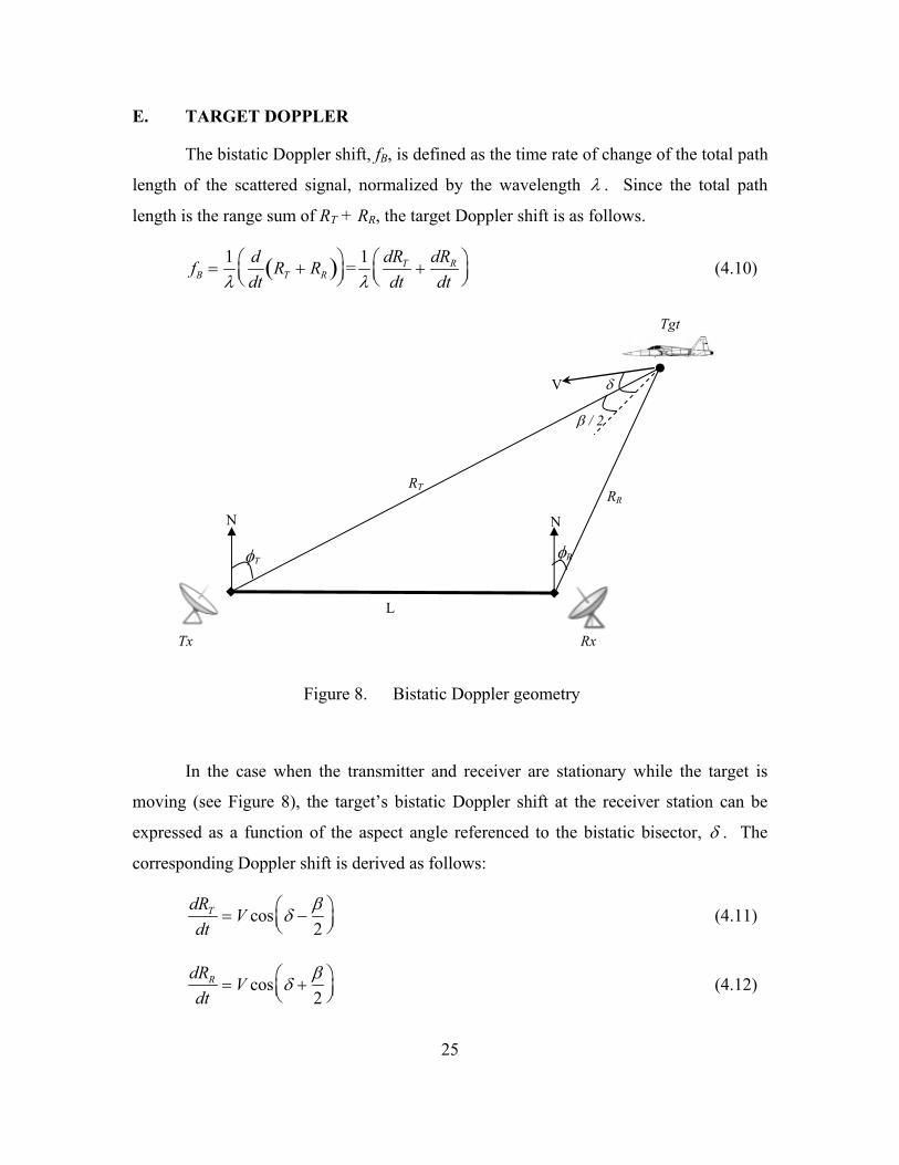
E. TARGET DOPPLER

The bistatic Doppler shift, fB, is defined as the time rate of change of the total path

length of the scattered signal, normalized by the wavelength λ . Since the total path

length is the range sum of RT + RR, the target Doppler shift is as follows.

fB =1λ

ddt

RT + RR( )

=1λ

dRT

dt+

dRR

dt

(4.10)

Figure 8. Bistatic Doppler geometry

In the case when the transmitter and receiver are stationary while the target is

moving (see Figure 8), the target’s bistatic Doppler shift at the receiver station can be

expressed as a function of the aspect angle referenced to the bistatic bisector, δ . The

corresponding Doppler shift is derived as follows:

dRT

dt= V cos δ −

β2

(4.11)

dRR

dt= V cos δ +

β2

(4.12)

Tx Rx

β / 2

Tgt

L

RT RR

N N

φR φT

δV

26

fB =Vλ

cos δ −β2

+ cos δ +

β2

⇒ fB =2Vλ

cos(δ )cosβ2

(4.13)

The properties of Equation (4.13) are presented in Table 1.

Condition Property All β Magnitude of the bistatic target Doppler shift is never greater than

that of the monostatic target Doppler shift, when the monostatic radar is located on the bistatic bisector.

All β -90° < δ < +90°

Bistatic target Doppler shift is positive.

All β δ = ±90°

Bistatic Doppler shift is zero.

All β < 180° δ = 0° or 180°

Target’s velocity is collinear with bistatic bisector. Magnitude of bistatic target Doppler shift is maximum.

β = 180° Target is on the baseline, characterized by large forward scatter. Radar can only detect presence of a target, the range is indeterminate due to eclipsing of the direct pulse by the scattered pulse.

Table 1. Properties of bistatic Doppler shift under various conditions (From [22])

F. DOPPLER RESOLUTION

For both monostatic and bistatic radars, the Doppler resolution depends on the

amount of Doppler separation between two target echoes at the receiver, fB1 and fB2. It is

accepted to be 1/T, where T is the receiver’s coherent processing interval [20]. Hence,

the requirement for Doppler resolution is

fB1 − fB2 =1T

(4.14)

In the bistatic case, an example of the geometry for two targets is as shown in

Figure 9. These targets are assumed to be collocated; consequently, they share a common

bistatic bisector. The corresponding bistatic target Doppler shifts are

27

Tx Rx

β / 2

Tgt #1, #2

L

RT RR

δ1

δ2

V1

V2

fB1=2V1

λcos(δ1)cos

β2

fB2 =2V2

λcos(δ2 )cos

β2

Combining these equations, the bistatic Doppler resolution can be obtained from

the difference between the two target velocity vectors, projected onto the bistatic bisector.

∆V = V1 cos(δ1) −V2 cos(δ2 )

⇒ ∆V =λ

2Tcos β2

(4.15)

Figure 9. Bistatic Doppler resolution (for 2 collocated targets)

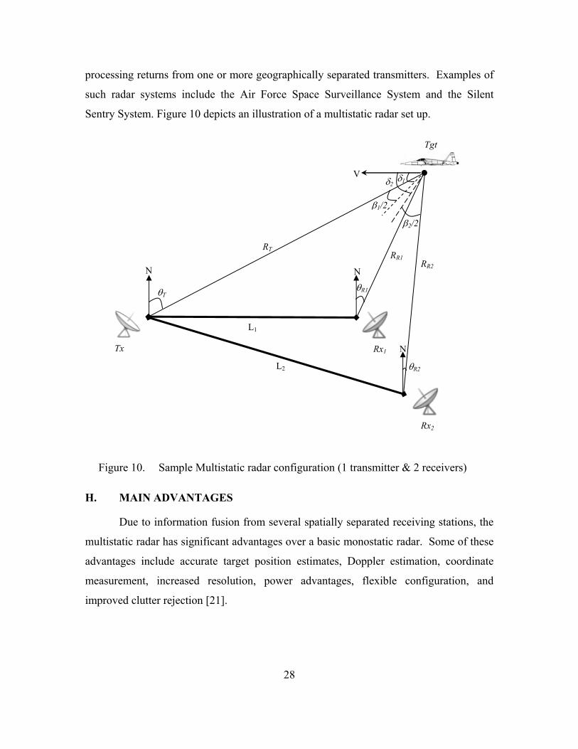
G. DEFINITION OF MULTISTATIC RADAR

The IEEE Standard 686-1997 [1] has defined the multistatic radar as a radar

system having two or more transmitting or receiving antennas with all antennas separated

by large distances when compared to the antenna sizes. It comprises at least three

components - one transmitter and two receivers, or multiple receivers and multiple

transmitters. It is an extension of the bistatic radar system, with one or more receivers

28

processing returns from one or more geographically separated transmitters. Examples of

such radar systems include the Air Force Space Surveillance System and the Silent

Sentry System. Figure 10 depicts an illustration of a multistatic radar set up.

Figure 10. Sample Multistatic radar configuration (1 transmitter & 2 receivers)

H. MAIN ADVANTAGES

Due to information fusion from several spatially separated receiving stations, the

multistatic radar has significant advantages over a basic monostatic radar. Some of these

advantages include accurate target position estimates, Doppler estimation, coordinate

measurement, increased resolution, power advantages, flexible configuration, and

improved clutter rejection [21].

Tx Rx1

β1/2

Tgt

L1

RT RR1

N N

θR1 θT

δ1

L2

Rx2

N

θR2

RR2

β2/2

V δ2

29

1. Accurate Position Estimate of Targets

In a conventional monostatic radar, target position determination is more accurate

in down-range than in cross-range direction. The multistatic radar allows the estimation

of the target coordinates through range-sum measurements relative to the spatially

separated transmitting and receiving stations.

The track update rate may usually be higher in a multistatic radar than in a

monostatic radar, and consequently, higher tracking accuracy can be achieved.

2. Doppler Estimation of Target Velocity and Acceleration

Doppler frequency shifts measured at the various receiving stations allow the

estimation of the target’s velocity vector. With Doppler information, trajectory

information of a target can be estimated with accuracy in a short time interval. The use

of Doppler frequency shifts for velocity and acceleration estimates improve tracking

accuracy and general quality of the tracking process.

3. Measurement of Three Dimensional Coordinates and Velocity

Monostatic or bistatic radars can only determine the signals’ Directions Of

Arrival (DOA) based on the bearings of the radiation sources. Multistatic radars can

obtain the three-dimensional coordinates and their derivatives by triangulation,

hyperbolic methods, or their combination. Triangulation determines the position based

on the intersection of DOA from various receiving stations. The hyperbolic method

determines the position based on the intersection of hyperboloids of revolution, which

have their foci at receiving stations. A fixed Time Difference Of Arrival (TDOA) at a

pair of stations determines a hyperboloid of revolution on which surface the target must

lie. This TDOA is estimated by the signal delay in one station, which is necessary to

maximize the mutual correlation of signals received by the two stations [21].

The measurement of Doppler frequency shifts of the mutual correlation function

of signals received by a pair of receiving stations from a moving target allows the

multistatic radar to estimate the radial velocity relative to these stations. A multistatic

30

radar system comprising four or more stations will be able to obtain all three components

of the target velocity vector by Doppler frequency shift measurements.

4. Increased “Signal Information” of Target Body

“Signal information” [21] refers to the information extracted from target echoes

that concerns geometrical, physical and other features such as movement relative to target

center of mass. When a target is observed by a multistatic radar system from different

directions simultaneously, the total amount of signal information may be significantly

more substantial than that from a monostatic radar. With the signals received by spatially

separated receiving stations, the size, form and relative motion of a target can be

measured with higher accuracy and in a shorter time interval. Additionally, two-

dimensional and even three-dimensional radar images of the target can be obtained if the

transmitting and receiving stations are spatially coherent.

5. Increased Resolution

The radar’s resolution capability in measuring a target’s range, bearing or velocity

is related to the extent of the response of echo from a point target. High resolution

information of the target may be achieved in a multistatic radar system if the signals at

the receiving stations are spatially correlated. Using the hyperbolic method, these signals

undergo correlation processing and two sources of mutually uncorrelated radiations,

located within the main lobe of the receiving station’s antenna, can be resolved by the

system.

6. Power Advantages

The multitude of transmitting and receiving stations in the multistatic radar

system has additional power advantages compared to monostatic radar. Each receiving

station can exploit the energy transmission from all transmitting stations and enjoy

significant power benefits. When the baseline distances are adequately long, scattered

signal fluctuations are statistically independent at different receiving stations.

Information fusion may lead to additional power gain due to fluctuation smoothing.

Additionally, when stations are separated such that the angle between directions from a

31

target to a transmitting and a receiving station approaches 180°, the radar cross section

(RCS) and the scattered signal intensity may increase significantly at the receiving

stations. This increase in RCS cannot be completely reduced by stealth technologies such

as body shaping and application of radar absorbent material coating. Furthermore, since

the transmitter and receiver are spatially separated, receiver protection devices such as

duplexer and circulator are not required. Consequently, signal power losses are reduced.

7. Configurable Coverage Area

System geometry and fusion algorithms in a multistatic radar system permit the

extension of coverage area in the required direction. If the radar system is comprised of

mobile transmitter and/or receiver units, the reconfiguration of coverage area can be

achieved easily.

8. Improved Clutter Rejection

In a multistatic radar system, since the transmitting and receiving stations are

physically separated, the intersection volume of their main beams may be much less than

the main beam volume of a monostatic radar. Under certain conditions, a significant

reduction in clutter intensity can result. Additionally, moving target indication (MTI)

techniques perform better in a multistatic radar than a monostatic radar. When the radial

velocity of a target relative to a monostatic radar is zero, MTI techniques are useless. In a

multistatic radar system, a moving target cannot generally present zero radial velocity to

several spatially located receiving stations. Similarly, the limitation of blind radial

velocities in a monostatic radar is overcome.

I. MAIN DRAWBACKS

With the increased number of stations and components in a multistatic radar, the

added complexities also impose difficulties in the implementation. Some of these

drawbacks include the requirement for synchronization and mutual alignment, the need

for direct line of sight between stations and targets, the need for data transmission lines,

and increased processing requirements [21].

32

1. Synchronization, Phasing and Transmission of Reference Signals

Synchronization between the transmitting, receiving stations and control center is

necessary for accurate target coordinate measurement by the hyperbolic methods. When

cooperative signal reception is used in the multistatic radar system, the receivers must

know the signal waveform sent out by the transmitting stations. This can be achieved by

signal transmission through the data transmission lines or transmission of synchronization

codes to correct frequency and signal waveform. For coherent signal processing, a

common reference frequency is required at each station to couple the transmitters’ and

receivers’ heterodyne frequencies.

2. Requirement for Direct Line of Sight between Stations and Targets

The coverage of a multistatic radar system is limited by the necessity for direct

lines of sight between stations and targets. If a target is not concurrently visible to

several transmitting and receiving stations, information fusion cannot be achieved. This

is an important constraint, especially for ground-based multistatic radar systems in the

detection of low-level targets.

3. Need for Data Transmission Lines

These data transmission lines are used for signal or data transmission from the

stations to the control center, as well as command and control information transmissions.

These transmission lines need to be protected against interference and direct physical

attacks.

4. Increased Processing Requirement

In a multistatic radar system, the significant increase in information from a target

as compared with a monostatic radar will require fast processors for processing these data

in real time. Additionally, the coordinate conversion of local radar data from each

receiving station into a common coordinate system and the interstation data association

between measurements impose added processing needs. Furthermore, geometrical and

tracking algorithms are also more complex than those applied in monostatic radars.

33

5. Need for Accurate Station Positioning and Mutual Alignment

The accurate fusion of target information from several spatially located stations

requires the precise knowledge of the stations’ positions and their alignment. Positions of

stationary stations can be obtained accurately by geodetic methods. However, the

determination of positions of mobile stations will require additional navigation methods

such as GPS information. Errors in station positions and their misalignment will lead to

systematic errors of target location determination.

J. IMPLEMENTATION REQUIREMENTS

It is important that signal synchronization and spatial coherence among

transmitting and receiving stations be established.

Signal synchronization is required between the transmitting station and receiving

station for range measurement [22]. Time synchronization can be accomplished by

receiving the signal directly from the transmitter. This transmitting signal can be sent

directly if an adequate line of sight exists between the transmitter and receiver, via land

line or other communication links if such line of sight cannot be achieved. For these

direct synchronization means, the implementation is relatively straightforward.

Establishing spatial coherence (amplitude and phase) between each transmitting

and receiving station, and the coherent combination of signals from all receiving stations

are essential for coherent multistatic radar operation [23]. For a ground-based multistatic

radar system, a viable solution is the establishment of suitable data links between the

elements and the central information center.

In general, a multistatic radar could be easily implemented when the positions of

all transmitting and receiving stations are at fixed locations.

For the purpose of this thesis research, it is assumed that only the synchronization

signal and Doppler shift information received by each receiving station are available to

the multistatic radar system for processing. Thus, the challenge is to resolve the

geometry and obtain accurate position and velocity details of the targets based on limited

amount of available information.

34


35

V. RADAR MODEL DESIGN

A baseline design and approach has been developed to demonstrate the concept of

high resolution imaging. The initial radar model is based on the basic multistatic radar

configuration presented in the preceding chapter, with additional parameters included to

aid in the derivation of the required parameters. Figure 11 depicts such a framework and

the corresponding parameters.

Figure 11. Framework for initial Multistatic radar model

A. ASSUMPTIONS

The radar system is assumed to use antennas with relatively low gain. Hence, the

wide beam width makes it unsuitable for direct measurement of target bearing. It is

believed that the implementation of such a system is feasible and the focus is on the

localization of the targets and the resultant formation of the target images.

T1

R1

R2

TGT

L1

L2

RR2 RR1RT1

θT1R1

θoff2 θoff1

θR1

θR2

β1 β2

φT1

φR1

φR2

θT1R2

δ2 δ1 V

φTgt

36

For the purpose of this thesis research, it is assumed that only the time

synchronization signal and Doppler shift information received by each receiving station

are available to the multistatic radar system for processing. With the time

synchronization signal, the range sum, RT + RR, could be derived. The Doppler shift will

result in the knowledge of the target’s velocity vector.

Since the focus of this thesis is a proof of concept, it is assumed that, for ease of

demonstration, the operational area of interest is a flat two-dimensional plane. After the

concept has been proven, the more realistic three-dimensional space can be extended in a

relatively straightforward manner.

The target is assumed to behave like a rigid body. Non-rigid bodies can be

modeled by multiple targets with varying velocity vectors.

A flat earth has also been assumed to simplify the derivation and demonstration.

B. MODEL NOTATIONS

The notations used in the subsequent derivation are presented in Table 2. Parameter Notation Description

Bearing φTgt ,φT 1,φR1,φR2 Heading using North-referenced coordinate system

Bistatic Angle β1,β2 Bistatic angle for each Transmitter-Target-Receiver

bistatic system

Aspect Angle δ1,δ2 Aspect angle of target relative to bistatic bisector for

each Transmitter-Target-Receiver bistatic system

Offset Angle θoff 1,θoff 2 Angle that baseline for each Transmitter-Target-

Receiver bistatic system makes with horizontal axis

Subtended Angle θR1,θR2 ,θT 1R1,θT 1R2 Angle subtended within each bistatic triangle

Range RT1, RR1, RR2 Range to target

Baseline Distance L1, L2 Separation between Transmitter and Receiver for each

Transmitter-Target-Receiver bistatic system

Target Velocity V Magnitude of target’s velocity

Table 2. Notations used in multistatic radar model

37

C. TARGET BEARING AND RANGE RELATIVE TO TRANSMITTER

In this section, the objective is to determine the position of the target relative to

the transmitter. Therefore, the parameters to be determined are: target’s bearing relative

to the transmitter φT 1 and the target’s relative range to the transmitter, RT1.

From Equation (4.3), the derivation of RT1 can be extended in the multistatic case

to include one for each of the two bistatic triangles.

RT =RT + RR( )2 − L2

2 RT + RR( )− L sin φT( ) (4.3)

For the multistatic radar model (see Figure 11), the baseline for each transmitter-receiver

pair may not be aligned with the horizontal axis; hence, additional offset angles need to

be considered for the correct derivation. The angle φT in the denominator of Equation

(4.3) will need to include θoff 1 and θoff 2 .

RT 1 =RT 1 + RR1( )2 − L1

2

2 RT 1 + RR1 − L1 sin φT 1 +θoff 1( )( ) (5.1)

RT 1 =RT 1 + RR2( )2 − L2

2

2 RT 1 + RR2 − L2 sin φT 1 +θoff 2( )( ) (5.2)

With the availability of time synchronization signals, ∆TD1 and ∆TD2 , the range

sums, RT1 + RR1, and RT1 + RR2, can be obtained as

RT 1 + RR1 = c∆T1 + L1 (5.3)

RT 1 + RR2 = c∆T2 + L2 (5.4)

Hence, by substituting Equations (5.3) and (5.4) into Equations (5.1) and (5.2), φT 1 can

be estimated by the numerical solution of

RT 1 + RR1( )2 − L12

2 RT 1 + RR1 − L1 sin φT 1 +θoff 1( )( )−RT 1 + RR2( )2 − L2

2

2 RT 1 + RR2 − L2 sin φT 1 +θoff 2( )( )= 0 (5.5)

38

Thereafter, RT1 can be obtained from either Equation (5.1) or (5.2).

D. TARGET BEARING AND RANGE RELATIVE TO RECEIVERS

Next, the positions of the target relative to the receivers need to be determined.

The parameters of interest are: target’s bearing relative to the receivers, φR1 and φR2 and

the target’s relative range to the receivers, RR1 and RR2. After RT1 and φT 1 have been

determined, RR1 and RR2 can be obtained by applying the cosine rule for each of the

bistatic triangles. Similar to the derivations for the transmitter, the offset angles due to

the different baseline positions have to be considered.

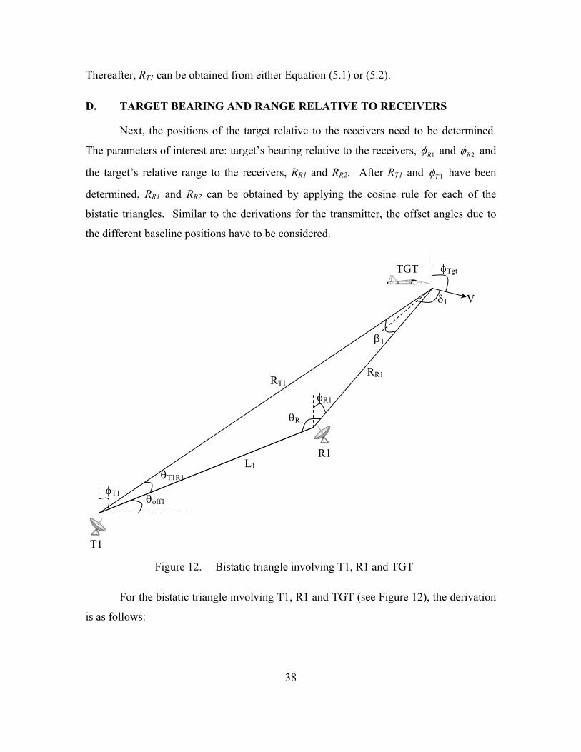
Figure 12. Bistatic triangle involving T1, R1 and TGT

For the bistatic triangle involving T1, R1 and TGT (see Figure 12), the derivation

is as follows:

T1

R1

TGT

L1

RR1RT1

θT1R1

θoff1

θR1

β1

φT1

φR1

δ1 V

φTgt

39

RR12 = RT 1

2 + L12 − 2RT 1L1 cos θT 1R1( ) (5.6)

Since θT 1R1 =π2−φT 1 −θoff 1 , therefore,

RR1 = RT 12 + L1

2 − 2RT 1L1 sin φT 1 +θoff 1( ) (5.7)

Using the cosine rule, β1 can be determined as

β1 = cos−1 RR12 + RT 1

2 − L12

2RR1RT 1

(5.8)

Thereafter, by the sine rule, θR1 can be derived as

θR1 = sin−1 RR1 sin(β1)L1

(5.9)

Hence, the bearing of the target relative to receiver R1 is

φR1 = φT 1 − β1 (5.10)

It should be noted that Equation (5.10) is only applicable in the case when the

target remains on the same side of the extended baseline of the Transmitter-Receiver pair.

If the target’s flight path is such that it crosses to the other side of the extended baseline,

then additional corrections will need to be done to obtain the correct bearing. This

situation of target traversing to the other side of the extended baseline will be seen when

the sum of the following angles exceed π / 2 .

When φT 1 +θT 1R1 +θoff 1 >π2

, then

θR1 = π −θT 1R1 − β1

φR1 =3π2−θoff 1 −θR1

Similarly, the parameters for second radar receiver, R2, are as follows:

RR2 = RT 12 + L2

2 − 2RT 1L2 sin φT 1 +θoff 2( ) (5.11)

40

β2 = cos−1 RR22 + RT 1

2 − L22

2RR2RT 1

(5.12)

φR2 = φT 1 − β2 (5.13)

E. TARGET VELOCITY VECTOR

The target’s velocity information can be extracted in two ways. Firstly, it can be

obtained from the Doppler shift information picked up by the receiving stations.

Secondly, with the derived target position information, a history track of the target can be

maintained and the corresponding velocity vector can be derived. The required

parameters are V, φTgt , and either δ1 or δ2 . The Doppler shift method will be discussed

first. The amounts of Doppler shift observed by the two receiving stations are:

fD1 =2Vλ

cos δ1( )cosβ1

2

(5.14)

fD2 =2Vλ

cos δ2( )cosβ2

2

(5.15)

By geometry (see Figure 11),

δ1 = δ2 +12β2 − β1( ) (5.16)

Substituting δ1 into Equation (5.14) and equating this with Equation (5.15), δ2 can be

found by the least-squares minimization search method such that δ2 will minimize the

following function.

f = fD1 cos δ2( )cosβ2

2

− fD2 cos

β2 − β1

2+ δ2

cosβ1

2

2

(5.17)

Following that, the magnitude of the target’s velocity V and its corresponding velocity

direction φTgt are derived.

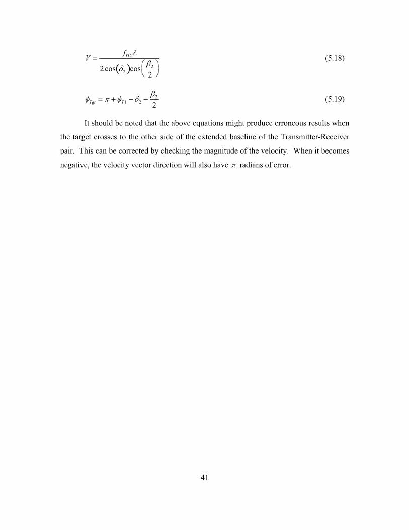
41

V =fD2λ

2cos δ2( )cos β2

2

(5.18)

φTgt = π + φT 1 − δ2 −β2

2 (5.19)

It should be noted that the above equations might produce erroneous results when

the target crosses to the other side of the extended baseline of the Transmitter-Receiver

pair. This can be corrected by checking the magnitude of the velocity. When it becomes

negative, the velocity vector direction will also have π radians of error.

42


43

VI. RADAR MODEL IMPLEMENTATION AND RESULTS

Based on the model introduced in the previous chapter, a procedure for

implementation will be described and presented in this chapter. The scenario is a

straightforward test case comprising one transmitter and two receivers. The results

obtained will include the target’s states (location and velocity) at each time step. These

will be analyzed and the errors will be examined in detail.

A. SCENARIO SETUP

Consider the case of a simple multistatic radar system comprising just one radar

transmitter (T1) and two radar receivers (R1 & R2), with two airborne targets (Tgt #1 &

#2) simulated to fly in different flight paths. Tgt #1 will fly in a sinusoidal path while

Tgt #2 will fly in a straight line. Figure 13 shows a schematic of this configuration.

Figure 13. Plan view schematic of scenario setup

The North referenced coordinate system will be adopted for the scenario, with the

origin fixed at the transmitter, T1. The coordinate positions for the transmitting and

receiving stations, as well as the start positions of the airborne targets are presented in

Table 3.

T1

R1

R2

Tgt #2

Tgt #1

44

Entity Position Parameters

Transmitter (T1) [0, 0] -

Receiver (R1) [50, 20] Baseline offset: θoff 1 = 21.8°

Receiver (R2) [100, 0] Baseline offset: θoff 2 = 0°

Target Initial Position

(Tgt #1)

[0, 100] Velocity: V1X = 100 m/s, V2Y =100 m/s

Target Initial Position

(Tgt #2)

[0, 100] Velocity: V2X = 100 m/s, V2Y = 0

Table 3. Radar stations and targets’ disposition and other parameters

In this setup, different target flight paths and different radar transmitter-receiver

baselines were tested for correctness of information extraction. T1 will transmit a CW

signal at a fixed frequency of 9 GHz to simulate a band-limited system. The time step

used is 1 ms and there are 3000 steps in each simulation run. This will translate to 3

seconds of target observation time.

B. TEST DATA GENERATION

For the purpose of the simulation, test data is divided into two categories: data

available to the radar system and data for results comparison and analysis.

1. Data Available to Radar System

From the assumptions for this thesis research, the radar system will only have two

sets of data: synchronization time delay and Doppler shift. In the simulation, these data

will be generated based on the flight paths and handed over to the radar processing

module to resolve the geometry and obtain accurate position and velocity details of the

targets.

2. Data for Results Comparison and Analysis

The data for results comparison are tabulated in Table 4. These data are

necessary to model each target at each time step.

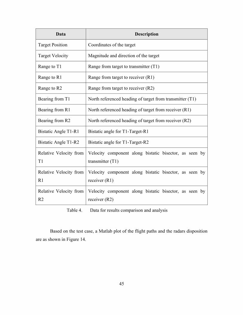
45

Data Description

Target Position Coordinates of the target

Target Velocity Magnitude and direction of the target

Range to T1 Range from target to transmitter (T1)

Range to R1 Range from target to receiver (R1)

Range to R2 Range from target to receiver (R2)

Bearing from T1 North referenced heading of target from transmitter (T1)

Bearing from R1 North referenced heading of target from receiver (R1)

Bearing from R2 North referenced heading of target from receiver (R2)

Bistatic Angle T1-R1 Bistatic angle for T1-Target-R1

Bistatic Angle T1-R2 Bistatic angle for T1-Target-R2

Relative Velocity from

T1

Velocity component along bistatic bisector, as seen by

transmitter (T1)


R1


receiver (R1)


R2


receiver (R2)

Table 4. Data for results comparison and analysis

Based on the test case, a Matlab plot of the flight paths and the radars disposition

are as shown in Figure 14.

46

0 50 100 150 200 250 300

0

50

100

150

200

Range (East Direction) [m]

Ran

ge (

Nor

th D

irect

ion)

[m]

Plan View of Radar Positions and Targets’ Flight Paths

T1

R1

R2

Tgt #1

Tgt #2

Figure 14. Radar positions and target flight paths

C. LEAST SQUARES IMPLEMENTATION

In the implementation of least squares analysis during radar measurement, the

data will be collected in blocks of 5 time steps and the least squares curve fit will be done

for each time block. Since each time step is 1 ms, the design matrix A employed initially

to solve Ax = m is in the form

A =

1 0.001 0.0012 0.0013

1 0.002 0.0022 0.0023

1 0.003 0.0032 0.0033

1 0.004 0.0042 0.0043

1 0.005 0.0052 0.0053

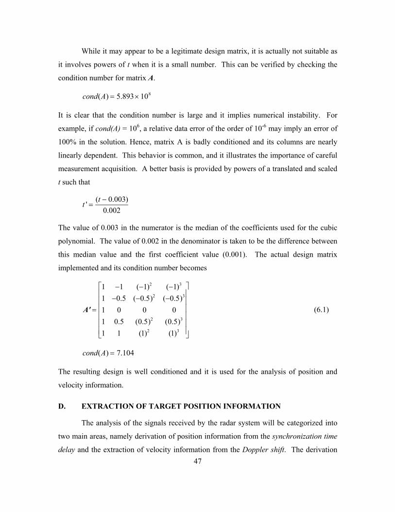
47

While it may appear to be a legitimate design matrix, it is actually not suitable as

it involves powers of t when it is a small number. This can be verified by checking the

condition number for matrix A.

cond(A) = 5.893×108

It is clear that the condition number is large and it implies numerical instability. For

example, if cond(A) = 106, a relative data error of the order of 10-6 may imply an error of

100% in the solution. Hence, matrix A is badly conditioned and its columns are nearly

linearly dependent. This behavior is common, and it illustrates the importance of careful

measurement acquisition. A better basis is provided by powers of a translated and scaled

t such that

t ' =(t − 0.003)

0.002

The value of 0.003 in the numerator is the median of the coefficients used for the cubic

polynomial. The value of 0.002 in the denominator is taken to be the difference between

this median value and the first coefficient value (0.001). The actual design matrix

implemented and its condition number becomes

A' =

1 −1 (−1)2 (−1)3

1 −0.5 (−0.5)2 (−0.5)3

1 0 0 01 0.5 (0.5)2 (0.5)3

1 1 (1)2 (1)3

(6.1)

cond(A) = 7.104

The resulting design is well conditioned and it is used for the analysis of position and

velocity information.

D. EXTRACTION OF TARGET POSITION INFORMATION

The analysis of the signals received by the radar system will be categorized into

two main areas, namely derivation of position information from the synchronization time

delay and the extraction of velocity information from the Doppler shift. The derivation

48

of target position information will involve the determination of transmitter to receiver

“round-trip” distance, target bearing and range relative to the transmitter, and target

bearing and range relative to the receivers.

1. Transmitter to Receiver “Round-trip” Distance

From the synchronization time delays, the “round-trip” range from transmitter to

target to receiver was first derived for each time step, target and radar transmitter-receiver

pair. The range was obtained by multiplying the time delay with the speed of light and

adding the baseline distance between the transmitter-receiver pair.

Range T1_Tgt1_R1 = Time Delay Tgt1_R1 * c + L1Range T1_Tgt2_R1 = Time Delay Tgt2_R1 * c + L1Range T1_Tgt1_R2 = Time Delay Tgt1_R2 * c + L2Range T1_Tgt2_R2 = Time Delay Tgt2_R2 * c + L2

(6.2)

For the test case, the two targets and two transmitter-receiver pairs will involve four sets

of “round-trip” ranges for time step.

2. Target Bearing and Range Relative to Receivers (R1 & R2)

With the target bearing and range relative to the transmitter known, the ranges of

the target relative to the receivers were obtained from Equations (5.7) and (5.11). Next,

the bistatic angles were derived from Equations (5.8) and (5.12). The bearings of the

target relative to the receivers were subsequently obtained from Equations (5.10) and

(5.13).

RR1 = RT 12 + L1

2 − 2RT 1L1 sin φT 1 +θoff 1( ) (5.7)

RR2 = RT 12 + L2

2 − 2RT 1L2 sin φT 1 +θoff 2( ) (5.11)

β1 = cos−1 RR12 + RT 1

2 − L12

2RR1RT 1

(5.8)

β2 = cos−1 RR22 + RT 1

2 − L22

2RR2RT 1

(5.12)

49

φR1 = φT 1 − β1 (5.10)

φR2 = φT 1 − β2 (5.13)

Plots of the measured values are shown in Figures 15 and 16.

0 50 100 150 200 250 300

0

50

100

150

200

Path of Tgt1 as seen from R1 (Measured)


Ran

ge (

Nor

th D

irect

ion)

[m]

T1

R1

R2

0 50 100 150 200 250 300

0

50

100

150

200



Ran

ge (

Nor

th D

irect

ion)

[m]

T1

R1

R2

Figure 15. Plot of Tgt #1 and Tgt #2 from measured data in Receiver R1

0 50 100 150 200 250 300

0

50

100

150

200



Ran

ge (

Nor

th D

irect

ion)

[m]

T1

R1

R2

0 50 100 150 200 250 300

0

50

100

150

200



Ran

ge (

Nor

th D

irect

ion)

[m]

T1

R1

R2

Figure 16. Plot of Tgt #1 and Tgt #2 from measured data in Receiver R2

In view of the lack of resolution in these figures, the graphical results appear to be

accurate enough for imaging purposes. Upon detailed comparison of each data point,

measurement errors can be calculated and analyzed. The average errors and

corresponding standard deviations of the measured results are tabulated in Table 5.

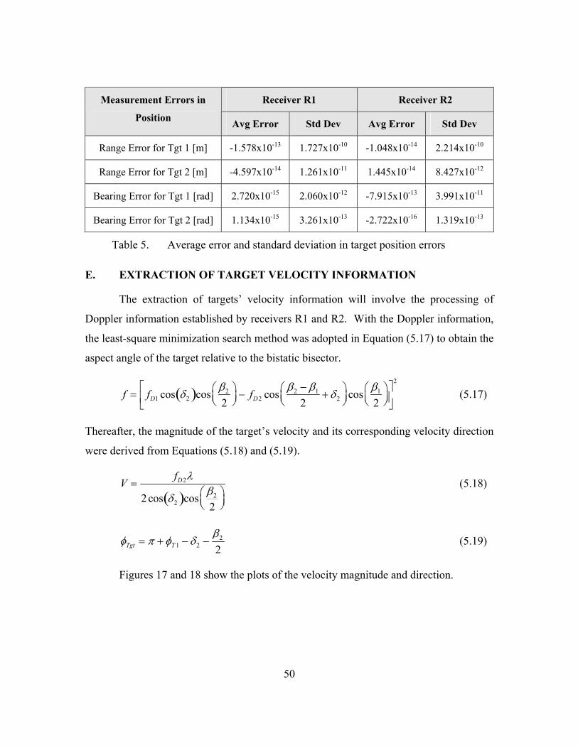
50

Receiver R1 Receiver R2 Measurement Errors in

Position Avg Error Std Dev Avg Error Std Dev

Range Error for Tgt 1 [m] -1.578x10-13 1.727x10-10 -1.048x10-14 2.214x10-10

Range Error for Tgt 2 [m] -4.597x10-14 1.261x10-11 1.445x10-14 8.427x10-12

Bearing Error for Tgt 1 [rad] 2.720x10-15 2.060x10-12 -7.915x10-13 3.991x10-11

Bearing Error for Tgt 2 [rad] 1.134x10-15 3.261x10-13 -2.722x10-16 1.319x10-13

Table 5. Average error and standard deviation in target position errors

E. EXTRACTION OF TARGET VELOCITY INFORMATION

The extraction of targets’ velocity information will involve the processing of

Doppler information established by receivers R1 and R2. With the Doppler information,

the least-square minimization search method was adopted in Equation (5.17) to obtain the

aspect angle of the target relative to the bistatic bisector.

f = fD1 cos δ2( )cosβ2

2

− fD2 cos

β2 − β1

2+ δ2

cosβ1

2

2

(5.17)

Thereafter, the magnitude of the target’s velocity and its corresponding velocity direction

were derived from Equations (5.18) and (5.19).

V =fD2λ

2cos δ2( )cos β2

2

(5.18)

φTgt = π + φT 1 − δ2 −β2

2 (5.19)

Figures 17 and 18 show the plots of the velocity magnitude and direction.

51

0 50 100 150 200 250 3000

50

100

150

200

250Velocity Magnitude of Tgt1 (Measured)


Mag

nitu

de [m

/s]

0 50 100 150 200 250 3000

20

40

60

80

100

120Velocity Magnitude of Tgt2 (Measured)


Mag

nitu

de [m

/s]

Figure 17. Velocity magnitude of Tgt #1 and Tgt #2 from measured data

0 50 100 150 200 250 3000

0.5

1

1.5

2

2.5

3Velocity Direction of Tgt1 (Measured)


Dire

ctio

n [r

adia

ns]

50 100 150 200 250 3001.5707

1.5708

1.5709Velocity Direction of Tgt2 (Measured)


Figure 18. Velocity direction of Tgt #1 and Tgt #2 from measured data

From these figures, it may appear that errors are more pronounced in Tgt #2 as

compared to Tgt #1. In reality, the errors for both targets are comparable and the

discrepancy is due to the limitation of resolution of the figures. The tabulated errors for

velocity magnitude and direction are tabulated in Table 6.

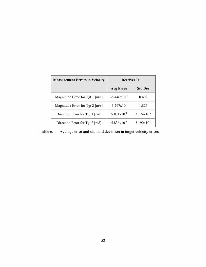
52

Receiver R1 Measurement Errors in Velocity

Avg Error Std Dev

Magnitude Error for Tgt 1 [m/s] -8.446x10-4 0.492

Magnitude Error for Tgt 2 [m/s] -3.297x10-2 1.826

Direction Error for Tgt 1 [rad] 5.834x10-4 3.174x10-2

Direction Error for Tgt 2 [rad] 5.836x10-4 3.190x10-2

Table 6. Average error and standard deviation in target velocity errors

53

VII. ERROR ANALYSIS

A. OVERVIEW

The errors arising as a result of the measurements can be broadly categorized into

four areas, namely position errors in range and bearing, and Doppler errors in velocity

magnitude and velocity direction. For each of these categories, the relevant

measurements are compared with the test data values, and the differences are treated as

errors and plotted. If the errors are significant, they will be manifested in the radar image

as imaging artifacts. Some of the significant errors in a noiseless environment are first

analyzed. They serve to illustrate the effect of the geometry of radar systems relative to

the targets. Although the measurements can be considered precise, the image errors can

still be significant if the condition number for the design matrix is large. Thereafter, the

errors with additive Gaussian noise are examined, so that the real world performance of

the system can be better understood.

B. ERRORS IN BEARING MEASUREMENT

For Receiver R1, Figure 19 presents the errors in bearing. It is evident that a

“spike” in error occurs at around 250 m. This occurrence can be explained by reviewing

the flight path of the target in relation to the disposition of the radar system. The

extended baseline of the transmitter-receiver pair for T1-R1 is as shown in Figure 20. It

is then obvious that the “spike” occurs at the intersection of this extended baseline with

the flight path of Tgt #2. This is reasonable for a bistatic radar since for the case when

the target lies on the extended baseline, the bistatic angle, β = 0 , and the error is

maximum. A similar “spike” was also observed in the errors for Tgt #1.

54

0 50 100 150 200 250 300−6

−5

−4

−3

−2

−1

0

1

2

3x 10

−12 Bearing Error of Tgt2 as seen from R1


Abs

olut

e E

rror

[rad

]

Figure 19. Bearing error for Tgt #2 as seen from receiver R1

0 50 100 150 200 250 300

0

50

100

150

200


Ra

ng

e (

No

rth

Dire

ctio

n)

[m]

Extended Baseline of T1−R1

T1

R1

R2

Tgt #1

Tgt #2

Figure 20. Extended baseline of Transmitter-Receiver pair for T1-R1

55

For Receiver R2, Figure 21 presents the errors in bearing. The “spike” occurs for

Tgt #1 for the similar reason highlighted for Receiver R1. Figure 22 depicts the

intersection of the extended baseline for Transmitter-Receiver pair T1-R2 with Tgt #1’s

flight path. Such “spikes” are not evident in Receiver R2 for Tgt #2 as its flight path

does not intersect the extended baseline.

0 50 100 150 200 250 300−2.5

−2

−1.5

−1

−0.5

0

0.5x 10

−9 Bearing Error of Tgt1 as seen from R2


Abs

olut

e E

rror

[rad

]

Figure 21. Bearing error for Tgt #1 as seen from receiver R2

56

0 50 100 150 200 250 300

0

50

100

150

200


Ran

ge (

Nor

th D

irect

ion)

[m]

Extended Baseline of T1−R2

T1

R1

R2

Tgt #1

Tgt #2

Figure 22. Extended baseline of Transmitter-Receiver pair for T1-R2

C. ERRORS IN VELOCITY MEASUREMENT

Figures 23 and 24 show the velocity magnitude errors. For Tgt #1, the error

“spikes” occur at ranges of about 80 m and 175 m. The first “spike” occurred when Tgt

#1 was turning back towards the South, and at about 80 m range, its aspect angle relative

to the radar system was 90 degrees. Consequently, there was a transition of the radial

velocity through zero and hence, there was a brief moment of zero Doppler shift. The

second “spike” occurred when Tgt #1 was at the extended baseline of the Transmitter-

Receiver pair T1-R1.

For Tgt #2, the error “spike” happens at about 50 m. This is a special case where

the target is traveling at the perpendicular bisector of the baseline of Transmitter-

Receiver pair T1-R2 with 90 degrees aspect angle. Consequently, there was zero

Doppler shift and the radar system responded with a “spike”. Figure 25 depicts the

erroneous regions for velocity magnitude measurements.

57

50 100 150 200 250 300−0.5

−0.4

−0.3

−0.2

−0.1

0

0.1

0.2

0.3

0.4

0.5Velocity Magnitude Error of Tgt1


Abs

olut

e E

rror

[m/s

]

Figure 23. Velocity magnitude error for Tgt #1

0 50 100 150 200 250 300−0.1

−0.08

−0.06

−0.04

−0.02

0

0.02

0.04

0.06

0.08

0.1Velocity Magnitude Error of Tgt2


Abs

olut

e E

rror

[m/s

]

Figure 24. Velocity magnitude error for Tgt #2

58

0 50 100 150 200 250 300

0

50

100

150

200


Ran

ge (

Nor

th D

irect

ion)

[m]

Erroneous Areas for Velocity Magnitude

T1

R1

R2

Tgt #1

Tgt #2

Figure 25. Erroneous regions for velocity magnitude measurements

D. ERRORS WITH ADDITIVE GAUSSIAN NOISE

For the purpose of concept demonstration, the errors analyzed so far have been

based on a noiseless environment. In actual radar operations, noise is an important factor

that cannot be neglected. Hence, the effect of noise on the radar model was tested with

additive Gaussian noise applied onto the synchronization signal and the Doppler shifts

measured by the radar system. The standard deviation used was two percent of the

measured signal. Figures 26, 27, 28, and 29 present samples of the errors for Tgt #1 with

additive Gaussian noise.

59

0 50 100 150 200 250 300−15

−10

−5

0

5

10

15

20

25Range Error of Tgt1 as seen from R1


Abs

olut

e E

rror

[m]

Figure 26. Range error for Tgt #1 as seen from receiver R1 (with 2% Gaussian noise)

0 50 100 150 200 250 300−1

−0.5

0

0.5

1

1.5

2

2.5

3Bearing Error of Tgt1 as seen from R1


Abs

olut

e E

rror

[rad

]

Figure 27. Bearing error for Tgt #1 as seen from receiver R1 (with 2% Gaussian noise)

60

0 50 100 150 200 250 30010

−2

10−1

100

101

102

103

104

105

106

Velocity Magnitude Error of Tgt1


Abs

olut

e E

rror

[m/s

]

Figure 28. Velocity magnitude error for Tgt #1 (with 2% Gaussian noise)

0 50 100 150 200 250 30010

−5

100

105

1010

1015

1020

Velocity Direction Error of Tgt1


Abs

olut

e E

rror

[rad

]

Figure 29. Velocity direction error for Tgt #1 (with 2% Gaussian noise)

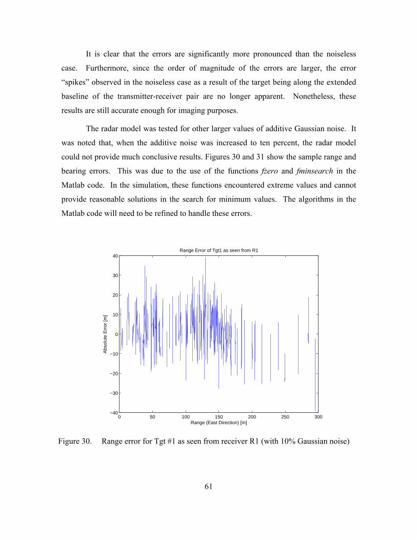
61

It is clear that the errors are significantly more pronounced than the noiseless

case. Furthermore, since the order of magnitude of the errors are larger, the error

“spikes” observed in the noiseless case as a result of the target being along the extended

baseline of the transmitter-receiver pair are no longer apparent. Nonetheless, these

results are still accurate enough for imaging purposes.

The radar model was tested for other larger values of additive Gaussian noise. It

was noted that, when the additive noise was increased to ten percent, the radar model

could not provide much conclusive results. Figures 30 and 31 show the sample range and

bearing errors. This was due to the use of the functions fzero and fminsearch in the

Matlab code. In the simulation, these functions encountered extreme values and cannot

provide reasonable solutions in the search for minimum values. The algorithms in the

Matlab code will need to be refined to handle these errors.

0 50 100 150 200 250 300−40

−30

−20

−10

0

10

20

30

40Range Error of Tgt1 as seen from R1


Abs

olut

e E

rror

[m]

Figure 30. Range error for Tgt #1 as seen from receiver R1 (with 10% Gaussian noise)

62

0 50 100 150 200 250 300−2.5

−2

−1.5

−1

−0.5

0

0.5x 10

4 Bearing Error of Tgt1 as seen from R1


Abs

olut

e E

rror

[rad

]

Figure 31. Bearing error for Tgt #1 as seen from receiver R1 (with 10% Gaussian noise)

Table 7 tabulates the standard deviation of the errors, taken to be the root mean

square deviation from the mean, as a result of various amounts of additive Gaussian

noise.

Gaussian

Noise

0.2% 0.5% 1.0% 1.5% 2.0% 3.0% 4.0% 5.0%

Range 0.4122 0.9378 1.4966 2.1441 2.8388 4.1039 5.6526 6.2225

Bearing 0.0242 0.0551 429.5414 392.2657 0.2024 0.3073 439.0524 0.5210

Velocity

Magnitude

373.7993 860.6418 1.5707e3 412.4362 543.7135 1.7291e13 794.3593 2.1248e4

Velocity

Direction

0.3124 0.4306 429.5287 392.2597 9.5243+13 1.8549e14 3.5188e14 3.3726e14

Table 7. Standard deviation of the different types of errors for various amounts of Gaussian Noise

63

Figures 32, 33, 34, and 35 plot these errors as a function of the amount of

Gaussian noise. It appears that the relationship between the standard deviation of range

errors is approximately linear to the amount of Gaussian noise added. This is rational

since the range errors are largely dependent on the errors in time synchronization only.

For the remaining three aspects, namely the bearing, velocity magnitude and velocity

direction errors, the coupling of the errors in the time synchronization with the errors in

the Doppler frequencies will generally result in larger deviations of errors.

0 0.5 1 1.5 2 2.5 3 3.5 4 4.5 50

1

2

3

4

5

6

7

Gaussian Noise [%]

Std

Dev

in R

ange

Err

or [m

]

Std Dev in Range Error for Various Amounts of Gaussian Noise

Figure 32. Standard deviation in range errors for various amounts of Gaussian noise

64

0 0.5 1 1.5 2 2.5 3 3.5 4 4.5 50

50

100

150

200

250

300

350

400

450

Gaussian Noise [%]

Std

Dev

in B

earin

g E

rror

[rad

]

Std Dev in Bearing Error for Various Amounts of Gaussian Noise

Figure 33. Standard deviation in bearing errors for various amounts of Gaussian noise

0 0.5 1 1.5 2 2.5 3 3.5 4 4.5 50

2

4

6

8

10

12

14

16

18x 10

12

Gaussian Noise [%]

Std

Dev

in V

eloc

ity M

agni

tude

Err

or [m

/s]

Std Dev in Velocity Magnitude Error for Various Amounts of Gaussian Noise

Figure 34. Standard deviation in velocity magnitude errors for various amounts of

Gaussian noise

65

0 0.5 1 1.5 2 2.5 3 3.5 4 4.5 50

0.5

1

1.5

2

2.5

3

3.5

4x 10

14

Gaussian Noise [%]

Std

Dev

in V

eloc

ity D

irect

ion

Err

or [r

ad]

Std Dev in Velocity Direction Error for Various Amounts of Gaussian Noise

Figure 35. Standard deviation in velocity direction errors for various amounts of Gaussian noise

66


67

VIII. RECOMMENDATIONS AND CONCLUSION

A. RECOMMENDATIONS FOR FUTURE WORK

1. More Complex Scenarios

The multistatic radar system analyzed thus far was based on the straightforward

disposition of one transmitter and two receivers. Although this was adequate for the

proof of concept of providing high-resolution imagery of airborne targets, the

employment of more transmitting and receiving stations can support more complex

treatment of image and error analysis. With more transmitter-receiver pairs, additional

algorithm can be applied to eliminate the error “spikes” and imaging artifacts.

Further, the scenario was tested based on simple two-dimensional geometry. A

more generalized analysis with a three-dimensional perspective could reveal issues and

challenges that degrade the performance of the imaging system. For instance, due to

symmetry, when conducting measurements using only Doppler information, a target

trajectory cannot be distinguished from its mirror image about a vertical plane that bisects

the baseline.

Consequently, as the scenario becomes more complex, the algorithm for the radar

model will need to be more robust to handle the increased complexity. For instance, the

limitations in the use of Matlab functions fzero and fminsearch need to be overcome to

handle scenarios with greater noise interference.

2. Performance in Real World Environment

The test data and measurements made in the test cases were simulated to be in a

noise-free environment. The inclusion of noise, clutter, and other environmental effects

such as multipath in the simulations will allow a more realistic analysis of the system’s

performance. Historically, multipath effects have prevented the exploitation of systems

using wide antenna beam widths for precision range instrumentation applications.

Another problem unique to multistatic sytems is multistatic ghosts, which arise when

using unaided multilateration techniques without transponders in a multitarget

68

environment [24]. These false target indications are generated when isorange contours

from two targets intersect at locations where no target exists. After considering these real

world effects, field testing of such a system will constitute an important component

towards verifying the performance of the radar system, as only then, can it be determined

whether this concept is practicable.

3. Analysis of Bistatic Ambiguity Function

Studies have shown that geometry plays an important role in the shape of the

bistatic ambiguity function as the system configuration is varied. For instance, analysis

in [25] has proposed algorithms to process the monostatic ambiguity function, and

thereafter, extract the bistatic factors. When the bistatic ambiguity function can be

determined reasonably well, the accuracy of the multistatic radar system can be

evaluated. Additionally, the conditions for imaging artifacts can be better understood,

and consequently, the artifacts can be eliminated more effectively.

B. CONCLUSION

The multistatic radar offers many advantages over monostatic radars in certain

applications, especially since the receiving stations can be located at covert and distant

sites relative to the transmitting stations. Furthermore, CW radars are relatively simple

and inexpensive to employ and maintain. Hence, a notional CW multistatic radar system

for high-resolution imaging was examined. This concept of using a Doppler-only

multistatic radar system to provide high resolution imaging of airborne targets was

demonstrated to be attainable. Through an understanding of conventional imaging

techniques and formulation of the inverse problem in radar imaging, the demonstration

radar model was designed to acquire an accurate position and velocity of the targets. The

extraction errors resulted from the range, bearing and velocity measurements were

congruent with the physical limitations of each transmitter-receiver pair. Using a

multistatic system, the geometrical diversity allowed these limitations to be overcome.

69

APPENDIX

% Matlab code for analysis of % High Doppler Resolution Imaging by Multistatic Continuous Wave Radars % using Constructive Techniques % % by Wei Ting Soh clear all; f = 9e9; % frequency lambda = 3e8 / f; % wavelength dt = 0.001; % time step Steps = 3000; % number of steps % Information Available to Radar %---------------------------------------------------------------------- % Radar Positions Num_Tx = 1; % number of transmitters Num_Rx = 2; % number of receivers xy_Tx = [0 0]; xy_Rx = [50 20; 100 0]; % Angle offset for diff Tx_Rx baseline to horizon, % and range between Tx and Rx theta_offset = zeros(Num_Rx); % offset angle for each baseline L = zeros(Num_Rx); % baseline distance theta_offset = atan((xy_Rx(:,2)-xy_Tx(2)) ./ (xy_Rx(:,1)-xy_Tx(1))); L = sqrt((xy_Rx(:,2)-xy_Tx(1,2)).^2 + (xy_Rx(:,1)-xy_Tx(1,1)).^2); % Targets Num_Tgt = 2; % number of targets xy0 = [0 100; 0 100]; v = [100 100; 100 0]; % SET UP OF TEST CASE %---------------------------------------------------------------------- % Data Parameters data_xy_tgt = zeros(Steps,Num_Tgt,2); % position of targets at each time step data_range_Tx = zeros(Steps,Num_Tgt,Num_Tx); % range of targets to Tx at each time step data_bearing_Tx = zeros(Steps,Num_Tgt,Num_Tx); % bearing of targets to Tx at each time step data_range_Rx = zeros(Steps,Num_Tgt,Num_Rx); % range of targets to Rx at each time step data_bearing_Rx = zeros(Steps,Num_Tgt,Num_Rx); % bearing of targets to Rx at each time step data_beta = zeros(Steps,Num_Tgt,Num_Rx); % bistatic angle of targets at each time step data_velocity = zeros(Steps,Num_Tgt,2); % velocity magnitude and direction of targets at each time step data_Vr_Tx1 = zeros(Steps,Num_Tgt,Num_Tx); % relative velocity of targets to Tx at each time step

70

data_Vr_Rx = zeros(Steps,Num_Tgt,Num_Rx); % relative velocity of targets to Rx at each time step % Information available to radar system time_delay = zeros(Steps,Num_Tgt,Num_Rx); % synchronization time delay from Tx to targets to Rx at each time step fd = zeros(Steps,Num_Tgt,Num_Rx); % Doppler shift of targets at each time step for k = 1:Steps; t = k * dt; for m = 1:Num_Tgt; % Target position data_xy_tgt(k,m,:) = xy0(m,:) + v(m,:) .* [t,sin(2*t)]; % Velocity if k >= 2 [theta, data_velocity(k,m,1)] = cart2pol((data_xy_tgt(k,m,1) - data_xy_tgt(k-1,m,1))/dt,(data_xy_tgt(k,m,2) - data_xy_tgt(k-1,m,2))/dt); if theta <= pi/2 % check for correct sector of velocity direction data_velocity(k,m,2) = pi/2 - theta; elseif (theta <= 1.5 * pi) and (theta > pi/2) data_velocity(k,m,2) = theta - pi/2; elseif (theta <= 2 * pi) and (theta > 1.5*pi) data_velocity(k,m,2) = 2.5*pi - theta; end; end; for n = 1:Num_Rx; % Relative range data_range_Tx(k,m,1) = sqrt((data_xy_tgt(k,m,2)-xy_Tx(1,2))^2 + (data_xy_tgt(k,m,1)-xy_Tx(1,1))^2); data_range_Rx(k,m,n) = sqrt((data_xy_tgt(k,m,2)-xy_Rx(n,2))^2 + (data_xy_tgt(k,m,1)-xy_Rx(n,1))^2); % Bearing (measured from North) data_bearing_Tx(k,m,1) = atan((data_xy_tgt(k,m,1)-xy_Tx(1,1))/(data_xy_tgt(k,m,2)-xy_Tx(1,2))); if (data_xy_tgt(k,m,2)-xy_Rx(n,2)) >= 0 % Tgt is in NE/NW quadrant data_bearing_Rx(k,m,n) = atan((data_xy_tgt(k,m,1)-xy_Rx(n,1))/(data_xy_tgt(k,m,2)-xy_Rx(n,2))); elseif (data_xy_tgt(k,m,1)-xy_Rx(n,1)) >= 0 % Tgt is in SE quadrant data_bearing_Rx(k,m,n) = pi/2 + atan(abs((data_xy_tgt(k,m,2)-xy_Rx(n,2))/(data_xy_tgt(k,m,1)-xy_Rx(n,1)))); else % Tgt is in SW quadrant data_bearing_Rx(k,m,n) = - pi/2 - atan(abs((data_xy_tgt(k,m,2)-xy_Rx(n,2))/(data_xy_tgt(k,m,1)-xy_Rx(n,1)))); end; % Beta angle

71

data_beta(k,m,n) = acos((data_range_Tx(k,m,1)^2 + data_range_Rx(k,m,n)^2 - L(n)^2) / (2 * data_range_Tx(k,m,1) .* data_range_Rx(k,m,n))); % Time delay (between Tx and Rx) time_delay(k,m,n) = (data_range_Tx(k,m,1) + data_range_Rx(k,m,n) - L(n)) / 3.0e8; % add 2% Gaussian noise to time delay time_delay(k,m,n) = time_delay(k,m,n) + 0.02*time_delay(k,m,n)*randn; % Relative velocity to Tx data_Vr_Tx1(k,m) = data_velocity(k,m,1) * cos(pi + data_bearing_Tx(k,m,1) - data_velocity(k,m,2)); % Doppler shift for Receivers data_Vr_Rx(k,m,n) = data_velocity(k,m,1) * cos(pi + data_bearing_Tx(k,m,1) - data_velocity(k,m,2) - data_beta(k,m,n)); fd(k,m,n) = (data_Vr_Tx1(k,m) + data_Vr_Rx(k,m,n)) / lambda; % add 2% Gaussian noise to Doppler shift fd(k,m,n) = fd(k,m,n) + 0.02*fd(k,m,n)*randn; end; end; end; % Plot scenario setup % figure; % plot(xy_Tx(1),xy_Tx(2),'kO',xy_Rx(:,1),xy_Rx(:,2),'bX',data_xy_tgt(:,1,1),data_xy_tgt(:,1,2),'r',data_xy_tgt(:,2,1),data_xy_tgt(:,2,2),'b'); % axis([-10 310 -20 210]); % xlabel('Range (East Direction) [m]'); % ylabel('Range (North Direction) [m]'); % title('Plan View of Radar Positions and Targets'' Flight Paths'); % text(-3,-8,'T1'); % text(47,12,'R1'); % text(97,-8,'R2'); % text(70,190,'Tgt #1'); % text(75,95,'Tgt #2'); % Show extended baseline for T1-R1 pair % figure; % plot(xy_Tx(1),xy_Tx(2),'kO',xy_Rx(:,1),xy_Rx(:,2),'bX',data_xy_tgt(:,1,1),data_xy_tgt(:,1,2),'r',data_xy_tgt(:,2,1),data_xy_tgt(:,2,2),'b'); % axis([-10 310 -20 210]); % xlabel('Range (East Direction) [m]'); % ylabel('Range (North Direction) [m]'); % title('Extended Baseline of T1-R1'); % text(-3,-8,'T1'); % text(47,12,'R1'); % text(97,-8,'R2'); % text(70,190,'Tgt #1'); % text(75,95,'Tgt #2'); % line([0 300], [0 120],'Color','m','LineStyle','-.'); % Show extended baseline for T1-R2 pair % figure; % plot(xy_Tx(1),xy_Tx(2),'kO',xy_Rx(:,1),xy_Rx(:,2),'bX',data_xy_tgt(:,1,1),data_xy_tgt(:,1,2),'r',data_xy_tgt(:,2,1),data_xy_tgt(:,2,2),'b');

72

% axis([-10 310 -20 210]); % xlabel('Range (East Direction) [m]'); % ylabel('Range (North Direction) [m]'); % title('Extended Baseline of T1-R2'); % text(-3,-8,'T1'); % text(47,12,'R1'); % text(97,-8,'R2'); % text(70,190,'Tgt #1'); % text(75,95,'Tgt #2'); % line([0 300], [0 0],'Color','m','LineStyle','-.'); % Show extended baseline for T1-R1 pair & perpendicular bisector for T1-R2 pair % figure; % plot(xy_Tx(1),xy_Tx(2),'kO',xy_Rx(:,1),xy_Rx(:,2),'bX',data_xy_tgt(:,1,1),data_xy_tgt(:,1,2),'r',data_xy_tgt(:,2,1),data_xy_tgt(:,2,2),'b'); % axis([-10 310 -20 210]); % xlabel('Range (East Direction) [m]'); % ylabel('Range (North Direction) [m]'); % title('Erroneous Areas for Velocity Magnitude'); % text(-3,-8,'T1'); % text(47,12,'R1'); % text(97,-8,'R2'); % text(70,190,'Tgt #1'); % text(75,95,'Tgt #2'); % line([0 200], [0 80],'Color','m','LineStyle','-.'); % line([50 50], [-10 120],'Color','m','LineStyle','-.'); % line([78 78], [170 210],'Color','m','LineStyle','-.'); % --------------------------------------------------------------------- % DATA PROCESSING AND SOLUTIONING x_scale = [0.1:0.1:300]'; % set correct scale for x-axis when plotting range_Tx = zeros(Steps,Num_Tgt,Num_Tx); % range of targets to Tx at each time step bearing_Tx = zeros(Steps,Num_Tgt,Num_Tx); % bearing of targets to Tx at each time step range_Rx = zeros(Steps,Num_Tgt,Num_Rx); % range of targets to Rx at each time step bearing_Rx = zeros(Steps,Num_Tgt,Num_Rx); % bearing of targets to Rx at each time step range_Tx_Rx = zeros(Steps,Num_Tgt,Num_Rx); % round trip range from Tx to Tgt to Rx at each time step %----------------- % round trip range from Tx to Tgt to Rx for m = 1:Num_Tgt; for n = 1:Num_Rx; % range of T1-Tgt-R1, T1-Tgt-R2 range_Tx_Rx(:,m,n) = time_delay(:,m,n) * 3.0e8 + L(n); end; end; %----------------- % for Tx % output: range_Tx(k,m,n) & bearing_Tx(k,m,n)

73

for m = 1:Num_Tgt; for k = 1:Steps; thetaT = @(x) (range_Tx_Rx(k,m,1)^2-L(1)^2) / (2 * (range_Tx_Rx(k,m,1) - L(1)*sin(x + theta_offset(1)))) - (range_Tx_Rx(k,m,2)^2-L(2)^2) / (2 * (range_Tx_Rx(k,m,2) - L(2)*sin(x + theta_offset(2)))); bearing_Tx(k,m,1) = fzero(thetaT,0); range_Tx(k,m,1) = (range_Tx_Rx(k,m,1)^2-L(1)^2) / (2 * (range_Tx_Rx(k,m,1) - L(1)*sin(bearing_Tx(k,m,1) + theta_offset(1)))) ; end; end; %---------------- % for all Rx % output - position: range_Rx(k,m,n) & bearing_Rx(k,m,n) % velocity: velocity(k,m,n,2) [magnitude & bearing] beta = zeros(Steps,Num_Tgt,Num_Rx); % Bistatic angle of targets for each Tx-Rx pair at each time step delta = zeros(Steps,Num_Tgt,Num_Rx); % Delta angle of targets for each Tx-Rx pair at each time step velocity_dop = zeros(Steps,Num_Tgt,2); % velocity magnitude and direction of targets at each time step for m = 1:Num_Tgt; for n = 1:Num_Rx; for k = 1:Steps; range_Rx(k,m,n) = sqrt(range_Tx(k,m,1)^2 + L(n)^2 - 2 * range_Tx(k,m,1) * L(n) * sin (bearing_Tx(k,m,1) + theta_offset(n))); beta(k,m,n) = acos((range_Rx(k,m,n)^2 + range_Tx(k,m,1)^2 - L(n)^2) / (2 * range_Rx(k,m,n) * range_Tx(k,m,1))); % angle Tgt-Tx_Rx theta_Tx_Rx = asin(range_Rx(k,m,n) * sin(beta(k,m,n)) / L(n)); if bearing_Tx(k,m,1) + theta_Tx_Rx + theta_offset(n) > pi/2 + 0.000001 theta_Rx = pi - theta_Tx_Rx - beta(k,m,n); bearing_Rx(k,m,n) = 1.5*pi - theta_offset(n) - theta_Rx; else bearing_Rx(k,m,n) = bearing_Tx(k,m,1) - beta(k,m,n); end; % velocity relative to each receiver d2 = @(x) (fd(k,m,1) * cos(x) * cos(beta(k,m,2)/2) - fd(k,m,2) * cos(0.5*(beta(k,m,2)-beta(k,m,1))+x) * cos(beta(k,m,1)/2))^2; delta(k,m,2) = fminsearch(d2,1); delta(k,m,1) = delta(k,m,2) + (beta(k,m,2)-beta(k,m,1))/2; velocity_dop(k,m,1) = fd(k,m,2) * lambda / (2 * cos(delta(k,m,2)) * cos(beta(k,m,2)/2)); velocity_dop(k,m,2) = pi + bearing_Tx(k,m,1) - delta(k,m,2) - beta(k,m,2)/2;

74

% process negative velocities if velocity_dop(k,m,1) < 0 velocity_dop(k,m,1) = abs(velocity_dop(k,m,1)); if velocity_dop(k,m,2) > pi velocity_dop(k,m,2) = velocity_dop(k,m,2) - pi; end; end; end; end; end; %---------------------------------------------------------------------- % Least square processing: Ax = B % Error calculation window = 5; soln_Range = []; soln_Bearing = []; Processed_Range = []; Processed_Bearing = []; Processed_VelMag = []; Processed_VelDir = []; error_Range = []; error_Bearing = []; error_VelMag = []; error_VelDir = []; % Design matrix A = []; for s = 1:window; tt = (s*dt - 0.003) / 0.002; % time scaling for better basis of design matrix A = [A; 1 tt tt^2 tt^3]; % design matrix end; for m = 1:Num_Tgt; for n = 1:Num_Rx; soln_Range = []; soln_Bearing = []; soln_VelMag = []; soln_VelDir = []; for l = 1:(window):3000; % divide entire range into blocks of 'window' B1 = []; % A * x1 = B1 B2 = []; % A * x2 = B2 B3 = []; B4 = []; for s = 1:window; % extract data for the window B1 = [B1; range_Rx(l+s-1,m,n)]; B2 = [B2; bearing_Rx(l+s-1,m,n)]; B3 = [B3; velocity_dop(l+s-1,m,1)]; B4 = [B4; velocity_dop(l+s-1,m,2)]; end; x1 = A * lsqr(A, B1, 1e-16); x2 = A * lsqr(A, B2, 1e-16); x3 = A * lsqr(A, B3, 1e-16); x4 = A * lsqr(A, B4, 1e-16);

75

soln_Range = [soln_Range; x1]; soln_Bearing = [soln_Bearing; x2]; soln_VelMag = [soln_VelMag; x3]; soln_VelDir = [soln_VelDir; x4]; end; Processed_Range(:,m,n) = soln_Range; Processed_Bearing(:,m,n) = soln_Bearing; error_Range(:,m,n) = soln_Range - data_range_Rx(:,m,n); error_Bearing(:,m,n) = soln_Bearing - data_bearing_Rx(:,m,n); % Receiver range/bearing errors figure; plot(x_scale,error_Range(:,m,n)); title(['Range Error of Tgt',int2str(m), ' as seen from R',int2str(n)]); xlabel('Range (East Direction) [m]'); ylabel('Absolute Error [m]'); figure; plot(x_scale,error_Bearing(:,m,n)); title(['Bearing Error of Tgt',int2str(m),' as seen from R',int2str(n)]); xlabel('Range (East Direction) [m]'); ylabel('Absolute Error [rad]'); end; Processed_VelMag(:,m) = soln_VelMag; Processed_VelDir(:,m) = soln_VelDir; error_VelMag(:,m) = soln_VelMag - data_velocity(:,m,1); error_VelDir(:,m) = soln_VelDir - data_velocity(:,m,2) % Doppler errors figure; plot(x_scale,error_VelMag(:,m)); title(['Velocity Magnitude Error of Tgt',int2str(m)]); xlabel('Range (East Direction) [m]'); ylabel('Absolute Error [m/s]'); figure; plot(x_scale,error_VelDir(:,m)); title(['Velocity Direction Error of Tgt',int2str(m)]); xlabel('Range (East Direction) [m]'); ylabel('Absolute Error [rad]'); end;

77

LIST OF REFERENCES

[1] IEEE Standard Radar Definitions, IEEE Std 686-1997, September 16, New York, 1997.

[2] C. Chua, “Doppler-Only Synthetic Aperture Radar,” M.S. thesis, Naval

Postgraduate School, Monterey, CA, USA, 2006. [3] B. Borden, Radar Imaging of Airborne Targets: A Primer for Applied

Mathematicians and Physicists, Taylor & Francis, 1999. [4] M. I. Skolnik, Introduction to Radar Systems, 2nd edition, McGraw-Hill, 2001. [5] J. P. Zwart, Aircraft Recognition from Features Extracted from Measured and

Simulated Radar Range Profiles, ASCI, The Netherlands, 2003. [6] “Radar,” class notes for PH 4274, Physics Department, Naval Postgraduate

School, Summer 2007. [7] H. Stark, Image Recovery Theory and Application, pp. 466-467. Academic Press

Inc., US, 1997. [8] J. B. Keller, “Inverse Problems,” The American Mathematical Monthly, Vol. 83,

No. 2, pp. 107-118, February 1976. [9] M. Bertero and P. Boccacci, Introduction to Inverse Problems in Imaging, pp. 5-

10. Institute of Physics Publishing, UK, 1998. [10] V. Maz’ya and T. Shaposhnikova, Jacques Hadamard, A Universal

Mathematician. American Mathematical Society and London Mathematical Society, 1998.

[11] G. E. Forsythe, M.A. Malcolm, and C. B. Moler, Computer Methods for

Mathematical Computations. Prentice-Hall, New Jersey, 1997. [12] M. Bertero and P. Boccacci, Introduction to Inverse Problems in Imaging, pp. 81-

86. Institute of Physics Publishing, UK, 1998. [13] A. Tarantola, Inverse Problem Theory and Methods for Model Parameter

Estimation, p. 57. Society of Industrial and Applied Mathematics. 2005. [14] B. Borden, “Mathematical Problems in Radar Inverse Scattering,” Institute of

Physics Publishing on Inverse Problems, Vol. 18, No. 1, February 2002.

78

[15] T. Tsao, M. Slamani, P. Varshney, D. Weiner, H. Schwarzlander, and S. Borek, “Ambiguity Function for Bistatic Radar,” IEEE Trans Aerospace and Electronic Systems, Vol. AES-33, pp. 1041-1051, 1997.

[16] C. J. Baker, H.D. Griffiths, I. Papoutsis, “Passive Coherent Location Radar

System. Part 2: Waveform Properties,” IEE Proceedings Online No. 20045083, 2005.

[17] M. C. Wicks, B. Himed, H. Bascom, and J. Clancy, “Tomography of Moving

Targets (TMT) for Security and Surveillance,” presented at Advances in Sensing with Security Applications, p. 3, Il Ciocco, Italy, July 2005.

[18] M. C. Wicks, B. Himed, H. Bascom, and J. Clancy, “Tomography of Moving

Targets (TMT) for Security and Surveillance,” presented at Advances in Sensing with Security Applications, p. 6, Il Ciocco, Italy, July 2005.

[19] N. J. Willis, Bistatic Radar, 2nd Edition, pp. 119-122, Technology Service

Corporation, Silver Spring, MD, 1995. [20] M. I. Skolnik, Radar Handbook, 2nd Edition, McGraw-Hill, USA, 1990. [21] V. S. Chernyak, Fundamentals of Multisite Radar Systems, Overseas Publishers

Association, Gordon and Breach Science Publishers, Singapore, 1998. [22] N. J. Willis, Bistatic Radar, 2nd Edition, pp. 86-90, Technology Service

Corporation, Silver Spring, MD, 1995. [23] N. J. Willis, Bistatic Radar, 2nd Edition, p. 195, Technology Service Corporation,

Silver Spring, MD, 1995. [24] N. J. Willis and H. D. Griffiths, Advances in Bistatic Radar, SciTech Publishing

Inc., USA, 2007. [25] M. H. Sargazi and A. Jafargholi, “Bistatic Ambiguity Function and DOA

Estimation for PCL radar,” presented at IEEE Asia Pacific Conference on Circuits and Systems, 2006.

79

INITIAL DISTRIBUTION LIST

1. Defense Technical Information Center Ft. Belvoir, Virginia

2. Dudley Knox Library Naval Postgraduate School Monterey, California

3. Professor James H. Luscombe Code PH/Lj

Naval Postgraduate School Monterey, California

4. Professor Brett Borden Code PH/Bb


5. Professor Donald L. Walters Code PH/We


6. Professor Yeo Tat Soon Director, Temasek Defence Science Institute

National University of Singapore Singapore

7. Tan Lai Poh Senior Admin Officer (MDTS), Temasek Defence Science Institute

National University of Singapore Singapore

8. Soh Wei Ting Ministry of Defence

Singapore

high doppler resolution imaging by multistatic continuous ... · report documentation page form ......

Documents