highway cost-benefit analysis system
TRANSCRIPT
HIGHWAY COST-BENEFIT ANALYSIS SYSTEM
Venkatramani Rajamohan
Thesis submitted to the
College of Engineering and Mineral Resources
at West Virginia University
in partial fulfillment of the requirements for
the degree of
Master of Science
In
Industrial Engineering
Majid Jaraiedi, Ph.D., Chair
Wafik Iskander, Ph.D.
David R. Martenelli, Ph.D.
Morgantown, West Virginia
1999
Keywords: Cost-Benefit Analysis, Red book, Life Cycle Cost Analysis, WVDOH
Copyright 1999 Venkatramani Rajamohan
Abstract
HIGHWAY COST-BENEFIT ANALYSIS SYSTEM
Venkatramani Rajamohan
In this research, a methodology for computing road user cost for various competingalternatives was developed. Also, a software was developed to calculate the road user cost,perform economic analysis and update cost tables. The methodology is based on the manualentitled “A Manual on User Benefit Analysis of Highway and Bus-Transit Improvements”which was published in 1977 by American Association of State Highway and TransportationOfficials. The report contains procedures for the calculation of the road user cost, performeconomic analysis and further update the cost tables as and when the latest Consumer PriceIndices and Producer Price Indices are available.
The software application has been developed in Visual Basic 5, which interact withthe cost tables, stored in MS-Excel workbook, according to the user inputs. The softwareapplication was later updated to Visual Basic 6 when it was installed at WVDOH. Thesoftware application consists of two module, 1) Road User Cost Application and 2)Economic Analysis. Module 1 consists of two sub-modules, Road User Cost Calculation andUpdate Cost Tables and Indices. The use of this software will result in the computation of theroad user cost and economic analysis in a more efficient manner. It enables the decisionmakers to rationally select the most desirable alternative for building and refurbishingsegments of public highways.
iii
Dedication
This Thesis is dedicated to Mother and Sri Aurobindo.
iv
Acknowledgements
I express my sincere gratitude to Dr. Majid Jaraiedi, for his continued guidance and
support during my Masters Program at West Virginia University. He was always available
for any suggestions that I sought. I would always remember the trips that I made with him to
Charleston.
I also thank Dr. Wafik Iskander, for his ideas and suggestions during the thesis. I
would thank him for going through my work meticulously and helping me to achieve
perfection.
I am highly indebted to Dr. David R. Martenelli, for his benevolence to fund me in
the later part of the thesis. I also appreciate his suggestions in the field of Transportation
Engineering.
Finally, I thank God for giving me supporting parents and sister, Subha, whose
inspiration are invaluable. I dedicate the thesis to my Family. I also thank my friends for
their support and encouragement.
v
Table of Contents
Title Page ................................................................................................................................... i
Abstract ..................................................................................................................................... ii
Dedication ................................................................................................................................ iii
Acknowledgements.................................................................................................................. iv
Table of Contents ...................................................................................................................... v
List of Figures ........................................................................................................................viii
List of Tables ........................................................................................................................... xi
Chapter 1: Introduction and Research Objectives..................................................................... 1
1.1 Background ......................................................................................................................... 1
1.2 Need for Research............................................................................................................... 5
1.3 Research Objectives............................................................................................................ 6
1.4 Research Methodology ....................................................................................................... 6
1.5 Organization........................................................................................................................ 7
Chapter 2: Literature Review.................................................................................................... 8
2.1 Road User Economic Analysis ........................................................................................... 8
2.2 The 1977 Manual .............................................................................................................. 11
Chapter 3: Methodology ......................................................................................................... 13
3.1 Definitions......................................................................................................................... 15
3.1.1 Economic Analysis Definitions............................................................................... 15
3.1.2 Traffic Characteristic Definitions............................................................................ 17
3.2 Benefits of Highway Improvement................................................................................... 20
3.3 Measurement of User Benefits (Costs) as Reported in the 1977 Manual......................... 20
vi
3.3.1 Basic Section Cost................................................................................................... 21
3.3.2 Accident Cost .......................................................................................................... 24
3.3.3 Intersection Delay Cost ........................................................................................... 25
3.3.4 Transition Cost ........................................................................................................ 29
3.4 One Way Versus Two Way Traffic .................................................................................. 29
3.5 The Effects of Highway Improvement ............................................................................. 30
3.6 Economic Analysis Technique as Reported in the Manual .............................................. 31
3.7 Example of a Highway Economic Analysis ..................................................................... 34
3.7.1 Calculation of the User Costs.................................................................................. 37
3.7.2 Calculation of the User Benefits ............................................................................. 39
3.7.3 Computation of the Present Value and Measures of Economic Desirability. ......... 39
3.8 Methodology Used in the Software .................................................................................. 42
3.9 Cost Updating Procedures................................................................................................. 43
3.9.1 Updating Running Cost Factors .............................................................................. 47
Chapter 4: Software Description and Usage........................................................................... 50
4.1 Software Development Tools ........................................................................................... 51
4.2 Software Description ........................................................................................................ 54
4.3 Database Description ........................................................................................................ 85
4.4 Internal Working and the File Structure ......................................................................... 101
4.5 Valid Ranges for Inputs and Parameters......................................................................... 102
4.6 Example .......................................................................................................................... 104
Chapter 5: Conclusions and Recommendations for Future Research................................... 108
5.1 Conclusions..................................................................................................................... 108
vii
5.2 Recommendations for Future Research .......................................................................... 109
References............................................................................................................................. 110
Appendix A: Software Manual ............................................................................................. 114
viii
List of Figures
Figure 3.1: Basic Section costs (B) for passenger cars on Multi-Lane highways. ................. 22
Figure 3.2: Costs due to stopping at intersections (excludes idling) ...................................... 27
Figure 3.3: Costs due to idling at intersections....................................................................... 28
Figure 3.4: Section transition costs. ........................................................................................ 30
Figure 4.1 The Welcome Screen (Welcome.frm) ................................................................... 54
Figure 4.2: The Road User Cost Application Screen (Frmroad.frm)...................................... 55
Figure 4.3: The Startup Screen (Startup.frm) ......................................................................... 56
Figure 4.4: The Number of Sections Screen (Noofsection.frm) ............................................. 57
Figure 4.5: The Main Screen (Mainscreen.frm) ..................................................................... 58
Figure 4.6: The Vehicle Mix Screen (Fmrvehiclemix.frm).................................................... 59
Figure 4.7: The Basic Section Cost for Passenger Cars Screen (Frmbasicsection.frm) ......... 60
Figure 4.8: The Travel Time Cost for Passenger Cars Screen (Traveltime.frm).................... 61
Figure 4.9: The Grade Cost for Passenger Cars Screen (Gradecost.frm) ............................... 62
Figure 4.10: The Curve Cost for Passenger Cars Screen (Curveform.frm)............................ 63
Figure 4.11: The Speed Change Cost for Passenger Cars Screen (Speedchange.frm) ........... 64
Figure 4.12: The Basic Section Cost for the Total Vehicle Mix Screen
(Frmcumulativebasicsection.frm) ........................................................................................... 65
Figure 4.13: The Accident Cost Screen (Accident.frm) ......................................................... 66
Figure 4.14: The Transition Cost Screen (Transition.frm) ..................................................... 67
Figure 4.15: The Intersection Delay Cost Due to Stopping Screen (Delaycosts.frm) ............ 68
Figure 4.16 The Intersection Delay Cost Due to Idling Screen (Idlingcosts.frm) .................. 69
Figure 4.17: The Total Cost Screen (Frmtotalcost.frm) ......................................................... 70
ix
Figure 4.18: View/Edit Results Screen (Outputcosts.frm) ..................................................... 71
Figure 4.19: The Open/Saveas Dialog Box ............................................................................ 73
Figure 4.20: Inputs for the Project Screen (Inputresults.frm) ................................................. 73
Figure 4.21: The Print Results Screen (Frmprint.frm)............................................................ 74
Figure 4.22: The View Results Screen (Viewresults.frm) ...................................................... 75
Figure 4.23: Opening an Existing File Screen (Open.frm) ..................................................... 76
Figure 4.24: The View/Update Indices Screen (Frmupdateindices.frm) ................................ 78
Figure 4.25: The Economic Analysis Screen (Frmeconomic.frm) ......................................... 79
Figure 4.26: The Economic Analysis for Uniform Increase or Decrease Screen
(Frmuniformnpv.frm).............................................................................................................. 80
Figure 4.27: The Input Data for Economic Analysis Screen (Frminput.frm)......................... 81
Figure 4.28: The Base or Alternative 0 Screen (Frmbase.frm)............................................... 82
Figure 4.29: The New Alternative Screen (Frmcurrent.frm) .................................................. 83
Figure 4.30: The Net Present Value Analysis Screen (Frmnpv.frm)...................................... 84
Figure A1: The Welcome Screen.......................................................................................... 116
Figure A2: The Road User Cost Application Screen............................................................ 117
Figure A3: The Startup Screen ............................................................................................. 118
Figure A4: The Number of Sections Screen ......................................................................... 119
Figure A5: The Main Screen................................................................................................. 120
Figure A6: The Vehicle Mix Screen..................................................................................... 121
Figure A7: The Basic Section Cost for Passenger Cars Screen............................................ 122
Figure A8: The Travel Time Cost for Passenger Cars Screen.............................................. 123
Figure A9: The Grade Cost for Passenger Cars Screen ........................................................ 124
x
Figure A10: The Curve Cost for Passenger Cars Screen ...................................................... 125
Figure A11: The Speed Change Cost for Passenger Cars Screen......................................... 126
Figure A12: The Basic Section Cost for the Total Vehicle Mix Screen............................... 126
Figure A13: The Accident Cost Screen ................................................................................ 128
Figure A14: The Transition Cost Screen .............................................................................. 129
Figure A15: The Intersection Delay Cost Due to Stopping Screen ...................................... 130
Figure A16: The Intersection Delay Cost Due to Idling Screen ........................................... 131
Figure A17: The Total Cost Screen ...................................................................................... 131
Figure A18: View/Edit Results Screen ................................................................................. 133
Figure A19: The Open/Saveas Dialog Box .......................................................................... 134
Figure A20: Inputs for the Project Screen ............................................................................ 134
Figure A21: The Print Results Screen .................................................................................. 135
Figure A22: The View Results Screen.................................................................................. 136
Figure A23: Opening an Existing File Screen ...................................................................... 137
Figure A24: The View/Update Indices Screen ..................................................................... 140
Figure A25: The Economic Analysis Screen........................................................................ 144
Figure A26: The Economic Analysis for Uniform Increase or Decrease Screen ................. 144
Figure A27: The Input Data for Economic Analysis Screen ................................................ 145
Figure A28: The Base or Alternative 0 Screen ..................................................................... 147
Figure A29: The New Alternative Screen............................................................................. 147
Figure A30: The Net Present Value Analysis Screen ........................................................... 148
xi
List of Tables
Table 3.1: Type of Costs That Might be Included in the Highway Transportation Cost
Analysis................................................................................................................................... 14
Table 3.2: Facility Data for the Example................................................................................ 35
Table 3.3: Traffic Data............................................................................................................ 37
Table 3.4: Calculation of Highway User Cost ........................................................................ 38
Table 3.5: User Benefit Calculations ...................................................................................... 40
Table 3.6: Calculation of Present Value of Project-Related Costs ......................................... 41
Table 3.7: Consumer and Wholesale Price Indices for January 1975 and May 1994 ............ 45
Table 3.8(a): Multiplier Formula for Updating Running Costs of Passenger Cars ................ 46
Table 3.8(b): Multiplier Formula for Updating Running Costs of Single Unit Trucks.......... 46
Table 3.8(c): Multipliers for Updating Running Costs of 3 S-2 Combination Trucks ........... 47
Table 4.1: Toolbox Controls Used in this Software ............................................................... 52
Table 4.2: Inputs for Basic Section Cost. ............................................................................. 105
Table 4.3: Inputs for Basic Section Cost for the Vehicle Mix.............................................. 105
Table 4.4: The Accident Cost Table ..................................................................................... 106
Table 4.5: Inputs for Transition Cost .................................................................................... 106
Table 4.6: Inputs for the Intersection Delay Cost ................................................................. 107
Table A1. Consumer Price Indices and their Identity Numbers ........................................... 141
Table A2. Producer Price Indices and their Identity Numbers ............................................. 142
Table A3. Accident Costs for the Year 1997........................................................................ 142
Table A4: Inputs for Basic Section Cost............................................................................... 150
Table A5: Inputs for Basic Section Cost for the Vehicle Mix.............................................. 151
xii
Table A6: The Accident Cost Table ..................................................................................... 151
Table A7: Inputs for Transition Cost .................................................................................... 152
Table A8: Inputs for the Intersection Delay Cost ................................................................. 152
1
Chapter 1: Introduction and Research Objectives
1.1 Background
The United States of America can be described as a “nation on wheels”. The
government has given the highest impetus to the growth of highways for they are the lifelines
of this country. The period from 1920 to 1970 might well be called the “automobile age” for
during this period highway transportation assumed a dominant role in America. This era is
also referred to as the Modern Highway Development era for the birth and development of
the modern Interstate Highway System.
“With the completion of the Interstate Highway System, highway agencies are
increasingly focussing attention on reconstruction and improvement of existing highway
systems. The new improvements to existing facilities are being subjected to maximum
scrutiny, and a formal economic evaluation of the economic impact is becoming
commonplace.”[Wright, 1996]
This report presents a methodology for calculating road user cost based on the 1977
Manual entitled “ A User Benefit Analysis for Highway and Bus Transit Improvements”. The
1977 Manual provides cost factors, nomographs, and guidelines for estimating the economic
effects of highway construction. These include most types of highway improvements, such as
curve elimination, widening or adding lanes, reducing gradients, new road construction, and
intersection controls. The question faced by highway planners is whether the benefits from
the reduced user costs for a certain highway exceed the costs required to produce these
benefits. Highway improvement alternatives may include:
• Construction of new Freeways, expressways, or roads without access control to
supplement or replace existing roads.
2
• Widening of existing roads or reconstruction to high geometric standards.
• Straightening or eliminating curves.
• Grade changes, and passing lanes or grades.
• Installing traffic control devices (e.g. signals, signs, barriers).
The 1977 Manual has various sets of nomographs that can be used to calculate the road
user cost in a step by step fashion. This Manual is based on the research conducted by the
Stanford Research Institute (SRI) under NCHRP Project 2-12, “Highway User Economic
Analysis”. It describes the theoretical basis for the methodology for economic analysis, the
basis of cost factors, and the techniques for constructing nomographs, all developed for use
in the Manual. The Manual provides step by step procedures and guidelines, cost factors,
nomographs and tables for estimating the economic effects of highway improvements on
highway users. The approach to highway improvements expounded in the Manual requires
division of highway projects into geometrically similar sections (or composites of several
similar sections) that can then be evaluated rapidly through the nomographs and tabular data
that are provided for several highway and vehicle types. A brief description of the Manual is
presented in Chapter 2.
Since highway projects are designed, constructed and operated with public funding, it is
critical that economic analysis be done with prudence. In addition to determining the best
project with maximum potential, economic analyses provide not only the present situation
but also the future of the project. The Intermodal Surface Transportation Efficiency Act
(ISTEA) emphasizes assessment of multimodal alternatives and demand management
strategies [Decorla-Souza et. al., 1997]. This emphasis has increased the need for planners to
provide good comparative information to decision-makers. Cost-Benefit analysis is a useful
3
tool for comparison of the economic worth of alternatives and evaluates the trade-off
between economic benefits and costs.
“Section 303,” Quality Improvement,” of the National Highway Designation Act,
amends Section 106 of Title23, United States Code (U.S.C.), by adding a new Subsection (e)
entitled “Life Cycle Cost Analysis (LCCA).” Title 23, U.S.C., Subsection 106(e)(1) now
directs the Secretary to program that requires States to conduct a life cycle cost analysis of
each NHS high cost ($25,000,000 or more) usable project segment. This subsection further
defines LCCA as “a process for evaluating the total economic worth of a usable project
segment by analyzing initial costs and discounted future cost, such as maintenance,
reconstruction, rehabilitation, resorting and resurfacing costs, over the life of a project
segment” [FHWA Policy Memorandum, 1996].
As used in the LCCA required by 23 U.S.C., 106(e), the following definitions are defined
in the FHWA Policy Memorandum in 1996:
“High Cost” refers to usable project segments estimated to cost $25 million or more.
“Usable Project Segment” refers to a portion of a highway which a state proposes to
construct, reconstruct or improve that when completed could be open to traffic independent
of some larger overall project. Such a “usable project segment” could be completed under a
single contract or in multiple phases over several years.
To decide between alternatives, sound economic decisions and detailed analysis are
required in order to make a choice. Cost effective choice over the life of the asset becomes
inevitable. Future high costs or short life of a project can offset low initial cost advantages.
The time value of money and well-recognized economic analysis procedures are important
4
considerations in the decision making process. Formal analysis using engineering economics
can provide an answer.
Engineering economics provide a way to choose between alternatives when the
expenditure of capital funds comes into play. Three basic steps are involved in conducting an
economic analysis [Stanford Research Institute, 1961]:
1) Identify and define the different alternatives among which a selection is to be made.
2) Identify and define the various elements or factors that may result in differences in
the cost of the alternatives and remove from further consideration all events that have
happened or may happen regardless of which alternative is selected.
3) Reduce all of the alternatives to a comparable basis by translating all of the applicable
factors to a common dollar base and then make a cost comparison among the
alternatives over time, considering the time value of money through the use of the
compound interest.
Life Cycle Cost Analysis is the most appropriate economic evaluation technique. This
analysis considers all the costs incurred in the life of a project. Two important definitions
follow:
Life Cycle Costing- Economic assessment of an item, area, system, or competing design
alternatives considering all significant costs of ownership over the economic life,
expressed in terms of equivalent dollars [Dell’Isola et. al., 1981].
Life Cycle Design- Analysis which considers the construction, operation, and
maintenance of a facility during its entire design life [Lindow, 1978].
5
Life Cycle Costs include all costs anticipated over the life of the facility. The
economic analysis requires identifying and evaluating the economic consequences of
various alternatives over time or the life cycle of the alternative [Peterson, 1985].
Costs incurred in the highway reconstruction include:
• Initial Construction Cost
• Maintenance Costs
• Residual Costs
• Road User Cost
• Right of Way Costs
1.2 Need for Research
This report is based on a project sponsored by the West Virginia Division of
Highways (WVDOH). The project involved development of turnkey software, based on the
1977 Manual to be used by the WVDOH to compute the road user cost for various projects.
The methodology described in the Manual is quite detailed and time consuming
leaving many avenues where the user can commit error. Also, reading the nomographs and
tables can be a cumbersome process because of the large amount of information to be
processed to calculate the total road user cost. The Division of Highways found it quite
necessary and important to develop a simplified software, which can be used to calculate
road user cost in a more efficient manner and have the capability to compare various
alternative scenarios.
6
1.3 Research Objectives
The objective of this research was to develop a user friendly computer package based
on the 1977 Manual. A complete package was to be developed such that the user can
compute the road user cost, do an economic analysis and update the costs to the current year
based on the latest costs available, taking into consideration both the time value of money
and inflation. The research also involved gathering information from WVDOH officials. The
research methodology is described in the next section.
1.4 Research Methodology
Based on the requirements and specifications decided based on discussion with
WVDOH officials, the application was decided to be developed using Microsoft’s Visual
Basic 5.This software is also called the front-end software because it interacts with the user
and the database. The software is versatile and has some of the latest features required for
client-server architecture. The database has been created in MS-Excel where all the data
required in calculating the user costs are stored. Visual Basic 5 forms a bridge between the
user and the database. It helps the user to retrieve necessary information depending on the
various choices for input and calculate total user costs for a project. User friendly screens
were developed for this purpose where the user can fill in the inputs. These inputs are
processed and required tables are referred to automatically to calculate the various
components of the road user cost.
7
1.5 Organization
The report consists of five chapters. Chapter 2 presents a review of the literature
regarding the basic work done in this field and the various software used by the departments
of transportation in different states. Chapter 3 presents the methodology followed and the
list of steps used to compute the road user cost. Chapter 4 consists of the software
description, the flowchart for the software, and its mode of operation. Chapter 5 summarizes
the conclusions drawn from this research. It also presents the future recommendations that
can be carried out on this research. The appendix includes the user manual for the software.
A diskette has been included that contains two files:
1) Sourcecode.zip-Contains all the Form files (.frm), Project files (.vbp), and the FRX files
(.frx) in a zipped format.
2) Help.txt-An ASCII file containing instructions for user to unzip the files in the
Sourcecode.zip and use the software.
8
Chapter 2: Literature Review
Highway user cost benefit analysis has been a hot topic of discussion for a long time.
Various federal laws have made it imperative to carry on economic analysis for projects
worth over twenty five million dollars. The National Cooperative Highway Research
Program is an organization carrying out research in the various fields like administration,
transportation planning, design, materials and construction, maintenance, traffic, soils and
geology and some special projects. They have sponsored some research in the field of
economics that comes under highway administration projects [NCHRP, 1998]. The 1977
Manual is also a product of the research sponsored by NCHRP. These projects are NCHRP
Projects 2-12 and 2-12/1 and were carried out at the Stanford Research Institute.
The next section gives a description of various software that have been developed for
the economic analysis applications. This chapter also gives a brief description of the 1977
Manual.
2.1 Road User Economic Analysis
This section presents various software that are available for performing various
aspects of economic analysis for highway construction and improvement.
1) MicroBencost- This software, also called Microcomputer Evaluation of Highway User
Benefit, is an effort to computerize the 1977 Manual (also known as the Red Book). The
research is Project 7-12 of NCHRP projects and has been conducted at the Texas A&M
Research Foundation under the supervision of Dr. William F. McFarland. The objective
of this project was to develop a comprehensive, user-friendly, portable microcomputer
program to conduct comprehensive highway user benefit-cost analysis. The program uses
9
support data that can be updated. The focus of the research was directed to analyses at a
research level and its immediate area impact. This project constituted review of
procedures used in the user cost-benefit analyses to identify data required for
determination of vehicle operating costs, accident reduction benefits, travel time values,
and other appropriate factors, limited updating of basic data, development of
microcomputer software to facilitate the analyses procedure and preparation of user
manual and software documentation. The MicroBENCOST software developed as part of
this project is capable of performing life cycle cost analysis for a variety of project types
and scope, using both default values and user-provided data inputs [NCHRP, 1993]. The
software is being enhanced under NCHRP Project 7-12(2) [17].
2) Highway Economic Requirements System (HERS)- The Highway Economic
Requirements System was designed to perform highway needs analyses that reflect both
the current condition of the highway system and the estimated costs and benefits of
potential improvements to the system. Jack Faucett Associates developed HERS with the
assistance of Urban Institute, Cambridge Systematics, Inc., and Bellomo-McGee, Inc.
(BMI). The system was developed for the Highway Needs and Investment Branch of the
Federal Highway Administration (FHWA) which is responsible for maintaining the
system. The system enables the user to better examine costs, benefits and national
economic implications associated with highway options. HERS uses the description of
the current state of the highway system contained in Highway Performance Monitoring
System (HPMS) database as a basis of all analyses. A comprehensive description can be
found in HERS Overview [FHWA, 1994], Users Guide [FHWA, 1995] and Technical
Report [FHWA, 1996].
10
3) Surface Transport Efficiency Analysis Model (STEAM)- This is an enhanced version
of a planning tool called Sketch Planning Analysis Spreadsheet Model (SPASM), that
was developed by the FHWA in 1995 to assist planners in developing the type of
economic efficiency and other evaluative information needed for comparing cross-modal
and demand management strategies. The software is based on the principles of economic
analysis, and allows the development of monetized impact estimates for a wide range of
transportation investments and policies [Decorla-Souza et. al., 1997].
4) StratBENCOST- This software is being developed by Hickling Lewis Brod Inc. as part
of the NCHRP Project 2-18/4. The model incorporates an analysis of the network of
highways and surrounding roads. The objective of the StratBENCOST model is to
present a methodology which allows strategic level planners to integrate highway user
costs and benefit –cost analysis into a broad based highway investment evaluation tool.
The model is based on NCHRP Project 2.18 which is entitled “Research Strategies for
Improving Highway User Cost-Estimating Methodologies” [18] and NCHRP Project
2.18/3 [19], entitled “Development of an Innovative Highway User-Cost Estimation
Procedure”. This software can be employed at the early stages of strategic planning. Its
key features include [19]:
• Demand estimation traffic models.
• Value of time models based on economic data.
• Vehicle operating cost models.
• Environmental effects.
• Construction and disruption costs.
• Risk analysis element to account for uncertainty.
11
• Economic evaluation criteria.
This project is still active and has not been published yet by NCHRP [NCHRP Project 2-
18/4].
2.2 The 1977 Manual
Economic analysis for highway improvement gained wide acceptance after the
publication of the AASHTOP “Red Book” [AASHTO, 1952] in 1952. The Red Book was
updated in 1960. Claffey presented an updated highway user cost factors and economic
analysis methodology in his report [Claffey, 1971]. “A Manual on User Benefit Analysis of
Highway and Bus-Transit Improvement” was published by the American Association of
State Highway and Transportation Officials (AASHTO) in 1977. The Manual was written to
update, extend and replace the 1960 AASHTO Report entitled “Road User Benefit Analysis
for Highway Improvements” [Anderson et. al., 1972]. The Manual is also based on NCHRP
Report 133 entitled “Procedures for Estimating Highway User Costs, Air Pollution and
Noise Effects” [Curry et. al., 1972], except for the detailed analysis of congestion or
queueing, air pollution and noise. It also describes current cost factors and short cut
procedures for dealing with various project types described in Winfrey’s “Economic
Analysis of Highways” [Winfrey, 1968], NCHRP Report 96, “Strategies for the Evaluation
of Alternative Transportation Plan” [Thomas et. al., 1970], NCHRP Report 122, “Summary
and Evaluation of Economic Consequences of Highway Improvements” [Winfrey, 1971],
and NCHRP Report 146, “Alternative Multimodal Passenger Transportation Systems-A
Comparative Analysis” [Frye, 1976].
The highway user cost factors in this Manual are shown as a function of either traffic
speed or of the ratio of traffic volume to highway capacity (V/C ratio). The highway and
12
traffic characteristics that define highway capacity and traffic speed can be translated into
these parameters through the use of the Highway Capacity Manual and other design and
traffic engineering references. The Manual does not include indirect economic effects such
as land values and growth.
The rationale behind such a comprehensive economic analysis is the achievement of
maximum service from a given investment. The need for economic analysis of highway
improvements was cogently put by the 1960 AASHTO report:
“The tenet that a profit should be returned on an investment applies equally as well
to highway projects as to general business ventures. It is unthinkable to enter a business
venture with only an estimate as to the initial cost. An estimate as to the continuing cost with
an appraisal to the amount of profit to be made is equally essential. For example, it would
be ridiculous for a railroad company in conducting business only the cost of the roadbed
and its upkeep. Any analysis of railroad costs necessarily includes the cost of operation,
maintenance, and depreciation of its rolling stock. In the same sense, the total cost of the
highway improvement is the cost to improve and maintain the cost of the highway and to
operate all the vehicles thereon. Thus the planning and the design of a highway, particularly
the selection of the route and choice between alternatives, can best be done, or have
decision aided, by calculating the costs of vehicle operation, accidents, maintenance, time
etc, in addition to calculating initial costs. These establish the economic desirability of any
highway improvement.” [AASHTO, 1952]
The emphasis of the 1977 manual is to help in conducting engineering economy
studies in evaluating relevant alternatives and constructive decision making with the public
money.
13
Chapter 3: Methodology
Economic analysis for highway projects was proposed as a decision making tool as
early as mid-nineteenth century and gained wide acceptance until after the publications of the
AASHTO “Red Book” [AASHTO, 1952] in 1952. The Red Book was updated in 1960 and
all literatures on economic analysis were refined. A Stanford Research Institute report
prepared for NCHRP served as a basis for the 1977 edition of the AASHTO Red Book. That
document, which contains unit highway user cost factors based on the 1975 levels of vehicle
performance characteristics and prices, remains the primary reference source for economic
analyses in the United States. It serves as the primary basis for the software developed for the
West Virginia Division of Highways.
Highway transportation cost is defined as the sum of the highway investment cost, the
maintenance and operating costs, and the highway user costs. Highway investment cost
includes the cost of right-of-way, engineering design, construction, traffic control devices
and landscaping. Maintenance cost is the cost of preserving a highway and keeping it in
serviceable condition. Operating costs include the costs of traffic control, lighting, and the
like.
Road user cost comprises a major part of the highway transportation costs. They
include motor vehicle operating costs, the value of travel time, and traffic accident costs.
Usually, only those operating costs that depend on the number of miles traveled, such as the
cost of fuel, tires, engine oil, maintenance and a portion of depreciation are included in the
highway economic analysis. Registration and parking fees, insurance premiums, and the time
dependent portion of depreciation may be excluded when estimating the reduction in user
14
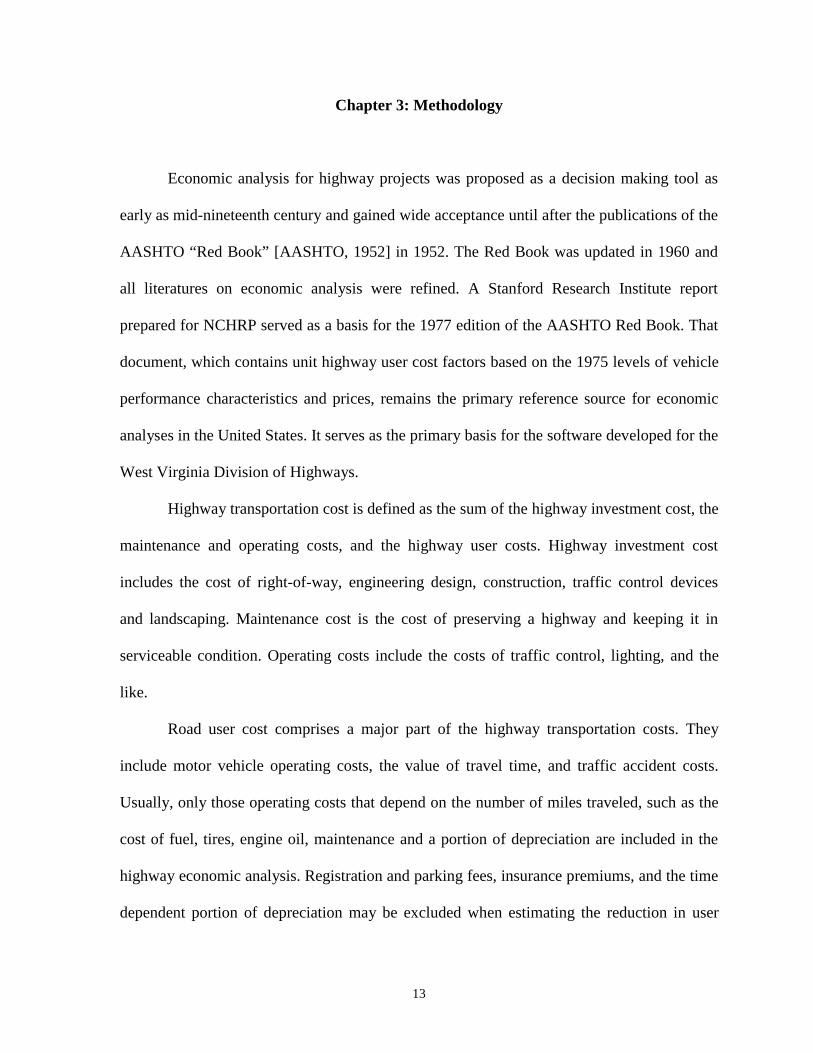
costs due to a highway improvement. Table 3.1 summarizes the components of highway
transportation costs.
Type of Cost Examples
Highway Investment CostsEngineering Design, Right of Way, Grading
and Drainage, Pavements.
Highway Maintenance Costs Mowing, Care of Roadside Parks, Lighting
Highway User Costs
a) Motor Vehicle Operating
Costs
Fuel, Lubrication, Tires.
b) Travel Time Total vehicle-hours of travel multiplied by unit
value of time.
c) Accident costs Estimated Accident Rate multiplied by Unit
Accident Cost.
Table 3.1: Type of Costs That Might be Included in the Highway Transportation Cost
Analysis
Economic studies for highway purposes are done principally for one or more of the
following reasons.
• To determine the feasibility of a project.
• To compare alternative configurations.
• To evaluate various features of highway design, for example, the type of surface to be
used.
15
• To determine the priority of improvement.
• To allocate responsibility for the costs of highway improvement among various classes of
highway users and some indirect benefit to non-users.
• Occasionally, to compare proposals for highway improvement with proposals for other
publicly funded projects.
3.1 Definitions
The definitions that follow include the principal technical terms used in the report and
have been adapted from the 1977 Manual. The listing is broken down into two categories:
economic analysis definitions and highway traffic characteristic definitions.
3.1.1 Economic Analysis Definitions
• Transportation Improvement Cost- The sum of investment cost, maintenance cost, user
costs, and transit user costs associated with a highway. The components of traffic
improvement costs are defined in the following sub-sections:
• Highway or Facilities Investment Cost- Total investment required for a highway
improvement, including engineering design and supervision, right of way acquisition,
construction, traffic control devices (signals and signs) and landscaping.
• Highway Maintenance Cost- The cost of keeping a highway and its appurtenances in
serviceable condition. Operating costs for traffic control and lighting should be
included with maintenance costs if operating costs differ appreciably between two
alternatives.
16
• Highway User Costs- The sum of 1) Motor vehicle running cost 2) The value of
vehicle user travel time, and 3) Traffic accident costs.
• Motor Vehicle Running Cost- The mileage dependent cost of running automobiles,
trucks, and other motor vehicles on the highway, including the expenses of fuel, tires,
engine oil, maintenance and that portion of the vehicle depreciation attributable to the
highway mileage traveled.
• Value of Travel Time- The result of vehicle travel time multiplied by the average unit
value of time.
• Vehicle Travel Time- The total vehicle hours of time traveled by a vehicle.
• Unit Value of Time- The value attributed to one hour of travel time, usually different
for passenger cars and trucks.
• Traffic Accident Cost- The costs attributable to motor vehicle traffic accidents
usually estimated by multiplying estimated accident rates by average cost per
accident.
• User Benefit- The advantages, privileges, and/or cost reductions that accrue to highway
motor vehicle users (drivers and owners). Benefits are generally measured in terms of a
decrease in user costs.
• Incremental Cost- The net change in dollar costs directly attributable to a given decision
or proposal compared with some other alternative (which could be existing condition or
do nothing alternative).
• Present Value (PV)- An economic concept that represents the translation of specified
amounts of costs or benefits occurring in different time periods into a single amount at a
single instant (usually the present). The term Net Present Value (NPV) refers to the net
17
cumulative present values of a series of costs and benefits stretching over time. It is
derived by applying to each cost or benefit in the series an appropriate discount factor,
which converts each cost or benefit to a present value.
• Equivalent Uniform Annual Cost (or Benefit)- A uniform cost (or benefit) that is the
equivalent, spread over the entire period of analysis, to all incremental disbursements or
costs incurred (or benefits received from) a project.
3.1.2 Traffic Characteristic Definitions
The following definitions refer generally tot the highway traffic characteristics.
• Capacity- Highway Capacity Manual defines capacity as the maximum number of
vehicles that have a reasonable expectation of passing over a given section of a lane or a
roadway in one direction or in both directions for a two-lane or three lane highway during
a given time period under prevailing roadway and traffic conditions. In the absence of
time modifier, capacity is expressed as an hourly volume.
• Passenger Car- A motor vehicle with a seating capacity of up to nine persons-including
taxicabs (for capacity and economy study purposes), station wagons, and two-axle, four
tire pickups, panels, and light trucks.
• Truck- A motor vehicle having dual tires on one or more axles, or having more than two
axles, designed for cargo rather than passengers. Two types of trucks are considered in
this report: 1) 12-kip, six tire, two axle single unit trucks and 2) 54 kip, diesel powered,
combination 3-S2 tractor semi-trailer trucks.
• Bus- A vehicle with seating capacity of ten or more passengers. Buses are usually
counted as single unit trucks for capacity and economic study purposes.
18
• Average Speed (or Average Overall Traffic Speed)- The summation of distances traveled
by all vehicles for a specified class of vehicles over a given section of highway during a
specified of time, divided by the summation of overall travel times.
• Overall Travel Time- The time of travel including stops and delays on the traveled way.
• Running Speed- The speed over a specified section of highway, equal to the distance
divided by the running time (the time the vehicle is in motion). Average Running Speed
is the same as the average speed if there are no stops; otherwise it is higher.
• Design Speed- A speed selected for the purposes of design and correlation of those
features of a highway, such as curvature, super-elevation, and sight distance, on which
the safe operation of a vehicle depends.
• Operating Speed- The highest overall safe speed at which a driver can travel on a given
highway under favorable weather conditions and under prevailing traffic conditions.
• Highway types- Four major highway types are considered in this report as described
below:
• Freeways and Expressways- Expressways are divided Arterials highways for through
traffic with full or partial control of access and generally with grade separations at
major intersections; Freeways are expressways with full control of access.
• Multi-Lane Highways- Roads with four or more lanes (that is two or more lanes in
each direction), without significant access control features and with low enough
adjacent development to permit speed limits of greater than 40 mph and signalization
with average spacing of more than one mile.
19
• Two-Lane Highways- Roads with two lanes (one in each direction), speed limit of
generally forty miles per hour in both directions, and average signal spacing more
than one mile. They may have varying degrees of access control.
• Arterials (or Arterial Streets, or Urban or Suburban Arterials)- Major streets and
highways outside the central business district having either 1) speed limits of 40 mph
or less and 2) average signal spacing of one mile or less.
• Average Annual Daily Traffic- The total yearly volume divided by the number of days in
a year, commonly abbreviated as AADT.
• Level of Service- A qualitative measure of the freedom of flow of traffic from
constraints, interruptions, or other inconveniences, relative to the best possible conditions
for a given type of highway facility. It is the inverse function of the hourly traffic volume
or the traffic density at the time of observation.
• Service Volume - The maximum number of vehicles that can pass over a given section of
a lane or a road-way in one direction on a Multi-Lane highway or Freeway (or in both
directions on a two-lane highway or three lane highway) during one hour while operating
conditions are maintained corresponding to the selected or specified level of service.
• Section- A “section” is defined as a road segment that possesses road characteristics
considered to be fairly homogeneous; it may be considered as the average of its smaller
subsections.
• Road Characteristic- The term “Road Characteristic” is defined as the various attributes
of a highway such as the grade percent or curve angle or the type of road surface.
20
3.2 Benefits of Highway Improvement
The benefits of highway improvement may be direct and readily apparent or may be
indirect and difficult to discern. Some benefits may be readily evaluated in monetary gains,
and some benefits may be intangible. For convenience, highway benefits have been grouped
into two categories.
1) Direct benefits that result from a reduction in highway user costs .
2) Indirect benefits, including benefit to adjacent property and the general public.
The most significant highway benefits are those that result from a reduction in the
user costs such as decreased operating costs, higher operating speeds, fewer delays, and
decreased accident losses.
3.3 Measurement of User Benefits (Costs) as Reported in the 1977 Manual
One of the most difficult aspects of economic analysis for highways is the
measurement of highway user benefits (costs). The highway user cost factors in the Manual
are shown as a function of either the traffic speed or of the ratio of traffic volume to highway
capacity (V/C ratio). The highway user costs for a given section of highway, HU, expressed
in dollars per thousand vehicles, is the sum of the Basic Section costs, accident costs, delay
costs and transition costs. The basic formula for computing highway user cost is as follows:
HU = (B+A) x L +T + D (3.1)
where,
B = Basic Section cost, consisting of the unit cost (time value and vehicle running costs) per
mile, associated with vehicle flow and basic geometric (grades and curves) of the analysis
section. The unit is dollars per 1000 vehicle miles.
21
A = Unit accident cost per mile in the analysis section. The unit is dollars per 1000 vehicle
miles.
L = Analysis section length in miles.
T = Transition cost; additional user unit time and running costs incurred due to changes in the
speeds between sections. The unit is dollars per 1000 vehicles.
D = Additional unit time and running cost due to delays at intersections, at traffic signals,
stop signs, or other traffic control devices. The unit is in dollars per 1000 vehicle.
In the following section, a summary of the methodology for calculating each of the
cost components is presented.
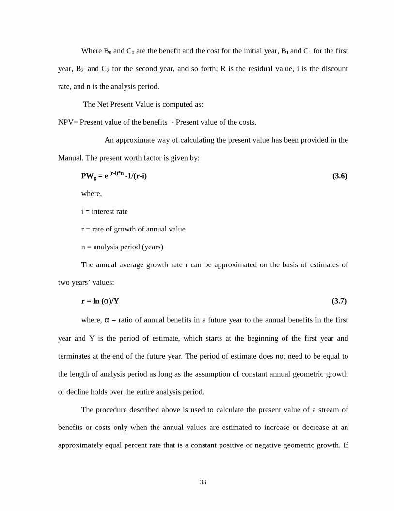
3.3.1 Basic Section Cost
The Manual gives the Basic Section costs in the form of nomographs for three classes
of vehicles: Passenger Cars, Single Unit Trucks and 3-S2 Combination Trucks, for four types
of highways: Freeways, Two-Lane Highway, Multi-Lane Highways and Arterial. Twelve
nomographs are used for the twelve combinations. As an example, one of these nomographs
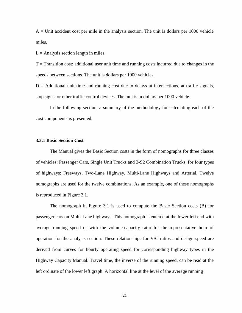
is reproduced in Figure 3.1.
The nomograph in Figure 3.1 is used to compute the Basic Section costs (B) for
passenger cars on Multi-Lane highways. This nomograph is entered at the lower left end with
average running speed or with the volume-capacity ratio for the representative hour of
operation for the analysis section. These relationships for V/C ratios and design speed are
derived from curves for hourly operating speed for corresponding highway types in the
Highway Capacity Manual. Travel time, the inverse of the running speed, can be read at the
left ordinate of the lower left graph. A horizontal line at the level of the average running
22
Figure 3.1: Basic Section costs (B) for passenger cars on Multi-Lane highways.
speed is then projected to the right scale to determine the tangent running cost (along a
specified grade) and added running costs due to curvature. Finally, additional running costs
due to speed change cycles are determined by entering the upper left graph with the volume-
capacity ratio and reading the added cost at the ordinate. The added cost due to the speed
change cycles is relatively small, except under the level of service F (or queueing)
conditions.
The Basic Section costs given in the example are valid only for the paved sections.
The cost of operating vehicles on gravel and stone roadway surfaces can be estimated by
multiplying the Basic Section costs from the nomograph by an adjustment factor. For
passenger cars, the adjustment factor ranges from 1.1 for a speed of 5 miles per hour to about
23
1.6 for the speed of 60 mph. Larger values are recommended for the single unit trucks and
combination trucks. The Basic Section cost has a unit of dollars per 1000 vehicle miles.
With a given V/C ratio and design speed, one can use the nomographs in Figures 7 to 18 of
the Manual (pp.50-61) to find the following costs:
a) Cost associated with the value of time.
b) Additional costs due to curvature.
c) Additional running cost due to grades.
d) Additional running cost due to speed changes.
The value of travel time is the product of the total vehicle hours of travel (by vehicle
type) and the average unit value of time. The magnitude of travel time depends on the
average running speed and the number and duration of stops. Studies have indicated that the
perceived value of travel time is sensitive to trip purposes and time savings per trip. The
travel time cost is in dollars per 1000 vehicle miles. The STEAM software uses a default
value of $6 per hour for passenger cars and $24.60 for commercial trucks as the values for
the travel time [Decorla et. al., 1997].
The cost of operating a vehicle on a straight or level tangent is related primarily to the
running speed and the gradient of the roadway. A gradient may be positive or negative.
Moving a vehicle up a steep positive grade requires more fuel than moving it along a level
road at the same speed. Sections with negative gradients can be negotiated with less burden
on the engine, but sometimes it may be necessary to apply brakes and that imposes added
running cost. These costs are accounted for under grade costs. The unit is dollars per 1000
vehicle miles.
24
Curves impose costs in addition to tangent road running costs through the centrifugal
force that tends to keep the vehicle following a tangent rather than a radial path. This force is
opposed by superelevation of the roadway and the side friction between the tire tread and the
road surface. There is a greater expenditure of energy and hence more fuel is required to
negotiate curved sections. The unit is dollars per 1000 vehicle miles.
Speed change costs are those incurred when the vehicle changes its speed from a high
value to a low value and goes back to the initial speed. The unit is expressed in dollars per
1000 vehicle miles.
3.3.2 Accident Cost
Accidents that occur every year on the streets and highways of America represent a
great economic loss beside the pain and suffering that they cause. Total economic loss
resulting from the motor vehicle accidents was estimated to be $156.6 billion in 1992
[Wright, 1996]. This total includes loss incurred in fatal accidents, accidents involving
nonfatal personal injury, and those involving only property damage. It follows that from an
economic standpoint, highway improvements cause a decrease in accident rates, resulting in
monetary saving to the road user and the public in general.
The accident cost can be reported in two ways.
1) The National Safety Council issues periodic report on the costs of vehicular
accidents. Once the types of accidents and their frequency are known, accident costs in
dollars per year can be calculated by multiplying the frequency (accidents per year) and the
cost per accident. Such costs include wage losses, medical expenses, property damages, and
insurance administration costs.
25
2) Unit accident costs can be estimated on the basis of empirical accident rates that
reflect regional effects of the vehicle mix, driver behavior, roadway type, and climate; or can
be estimated from the average rates and costs by accident types, as shown in Table 11 and
Table 13 of the Manual. The unit is expressed in dollars per 1000 vehicle miles.
To account for savings in accident costs in highway economic studies, accident rates
before and after the proposed improvement should be estimated. The analyst should be able
to rely on empirical data that will account for regional differences in vehicle mix, driver
behavior and climate.
3.3.3 Intersection Delay Cost
The most complex aspect of determination of the unit highway user costs is the
estimation of the cost of intersection delay (D). Two nomographs are published in the
Manual to determine intersection delay costs: one to estimate the unit costs of stopping at a
traffic signal and the other to estimate the unit costs of idling. In order to use these
nomographs, information on the following traffic and signalization parameters for the
intersection being studied are needed.
1) Green to cycle time ratio (λ). The ratio of the effective green time of the signal (generally
taken to be the actual green time) to the cycle length of the signal, both expressed in the same
unit of time (usually seconds).
2) Saturation flow (s). The approach volume in vehicles per hour of green for the intersection
when the load factor is 1.0 and the appropriate adjustment factors are applied. In the case of
absence of Highway Capacity Manual, recommended values of saturation flow are 1700 and
1800 vehicles per hour times the numbers of approach lanes.
26
3) Capacity (c). According to the Highway Capacity Manual, capacity is the service volume
of the approach at a load factor of 1.0. It is also equal to the saturation flow times the green-
to-cycle time ratio.
4) Degree of saturation (χ). The ratio of the volume of the traffic approaching the intersection
(usually in vehicles per hour) to the capacity of the intersection, in the same units.
5) Approach speed. Also termed mid-block speed, is the average running speed at which
the vehicle stream approaches the signalized intersection.
The degree of saturation is the ordinate of the left most graph of the nomograph (Figure 3.2).
For the given green to cycle time ratio, a line is projected on to the curve on the left most
graph to calculate the average stops per vehicle. This is then projected on to the middle graph
for the given approach speed, and the point at which it intersects the approach speed is
projected on to the ordinate to calculate the added stopping delay in hours per thousand
vehicles per signal. The same line is projected on to the right most graph to find the added
stopping cost per thousand vehicles per signal. The time cost is the additional delay due to
stopping multiplied by the hourly value of time per passenger car multiplied by the
adjustment factor for the trucks in the stream. The running cost for the intersection is the
additional stopping cost multiplied by the adjustment factor for the trucks in the traffic
stream.
27
Figure 3.2: Costs due to stopping at intersections (excludes idling)
The idling costs are found with the help of the idling cost nomograph (Figure 3.3).
The ordinate of the bottom most graph of the nomograph is entered for the given or
calculated degree of saturation. For the given capacity, the intersection point on the graph is
located and extended straight upwards to calculate the average delay per vehicle (seconds). A
small correction to average delay is also added for the given cycle length and green-to-cycle
ratio. This point is on the ordinate of the left upper most graph. It is extended to the right
hand side to calculate the idling time in hours per thousand vehicles and the idling costs in
dollars per 1000 passenger cars.
28
Figure 3.3: Costs due to idling at intersections
The total delay cost is the idling time multiplied by the hourly value of time per
passenger car and the adjustment factor for percent trucks in the stream. The total idling cost
is idling cost multiplied by the adjustment factor for the percent trucks in the stream. The
total cost due to idling per thousand vehicles per signal is the summation of the above costs.
The analysis of intersection delay often requires separate calculations for each direction of
approach, especially where opposing and /or crossing approaches have unequal traffic flows
or different characteristics (e.g., number and types of intersections, capacity, signalization
parameters, and so on). If there are three signalized intersections of approximately the same
characteristics included in the overall roadway being analyzed, one intersection might be
analyzed and the results multiplied by three. A degree of saturation of 1 implies that all
29
vehicles in the traffic stream would stop at the signal at least once and that average delay per
vehicle would at least equal the signal cycle time. The unit is expressed in dollars per 1000
vehicles.
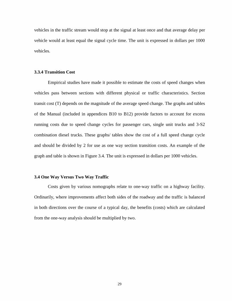
3.3.4 Transition Cost
Empirical studies have made it possible to estimate the costs of speed changes when
vehicles pass between sections with different physical or traffic characteristics. Section
transit cost (T) depends on the magnitude of the average speed change. The graphs and tables
of the Manual (included in appendices B10 to B12) provide factors to account for excess
running costs due to speed change cycles for passenger cars, single unit trucks and 3-S2
combination diesel trucks. These graphs/ tables show the cost of a full speed change cycle
and should be divided by 2 for use as one way section transition costs. An example of the
graph and table is shown in Figure 3.4. The unit is expressed in dollars per 1000 vehicles.
3.4 One Way Versus Two Way Traffic
Costs given by various nomographs relate to one-way traffic on a highway facility.
Ordinarily, where improvements affect both sides of the roadway and the traffic is balanced
in both directions over the course of a typical day, the benefits (costs) which are calculated
from the one-way analysis should be multiplied by two.
30
Figure 3.4: Section transition costs.
3.5 The Effects of Highway Improvement
Highway economic analyses should account for the changes in traffic volume that are
1) induced by the improvement, and 2) diverted from other routes to the new facility. It is,
therefore, recommended that the difference in the user benefits (costs) be multiplied by the
average of the traffic volume with and without the improvement.
User Benefits = (U0-U1) [(V0 +V1)/2] (3.2)
where,
U0 = user cost per unit of traffic (vehicles or trips) without the improvements.
U1 = user cost per unit of traffic with the improvement.
V0 = Level of the traffic without the improvement (AADT0)
31
V1 = Level of traffic with the improvement, including any induced or diverted traffic
(AADT1)
V1 may be larger than V0, as shown, or smaller when the traffic is diverted to any new
parallel facility.
3.6 Economic Analysis Technique as Reported in the Manual
Economic analysis intended to provide the economic justification for a particular
project or to permit comparison of alternative schemes or locations, in order to determine the
priority of improvement, etc. might be carried out by one of several methods. Methods used
in engineering economy studies include:
1) Benefit Cost ratio (B/C)
2) Net Present Value (NPV)
3) Comparison of annual costs
4) Determination of the interest rate (internal rate of return) at which the alternatives are
equally attractive.
Benefit Cost ratio (B/C) and the NPV methods are more commonly used by highway
engineers and administrators.
3.6.1 Benefit Cost Ratio
The following formulation of the benefit-cost ratio that utilizes the present values is
recommended for all highway and transit applications as an approximate indicator of the
project desirability.
B/C = PV (∆U)/[PV (∆I) +PV (∆M) -PV (∆R)] (3.3)
PV= The present value of the indicated amount or series.
32
∆U = User benefits, the reductions in the annual highway user costs due to the investment
(costs without the improvement less costs with the improvement).
∆I = Increased investment costs due to the project.
∆M = Increase in the series of the annual maintenance, operating, and administrative costs
due to the investment (costs with the improvement less costs without the improvement).
∆R= Increase in the residual value due to the project at the end of the effective life of the
project.
Example: If ∆U = $1000, ∆I = $900, ∆M = $-100, ∆R = 0 then B/C = 1000/900-100 =1.25
3.6.2 Net Present Value Method
The basic criterion for the economic desirability is that the present values of the
stream of annual benefits resulting from a project exceed the present value of the costs
associated with implementing the project. Since the Net Present Value (NPV) is defined as
the difference between the present value of the stream of benefits and the present value of the
stream of costs, an equivalent criterion or decision rule can be described as follows: if the
(NPV) associated with a particular improvement project or project alternative is greater than
zero, the project or the project alternative is economically justified.
NPV can be symbolically expressed as follows:
NPV = PV (∆U) + PV (∆R) - [PV (∆I) +PV (∆M)] (3.4)
Stated another way:
NPV = (B0 – C0) +(B1 – C1) / (1+i) +(B2 –C2) / (1+i)2 +……+(Bn –Cn +R) / (1+i) n (3.5)
33
Where B0 and C0 are the benefit and the cost for the initial year, B1 and C1 for the first
year, B2 and C2 for the second year, and so forth; R is the residual value, i is the discount
rate, and n is the analysis period.
The Net Present Value is computed as:
NPV= Present value of the benefits - Present value of the costs.
An approximate way of calculating the present value has been provided in the
Manual. The present worth factor is given by:
PWg = e (r-i)*n -1/(r-i) (3.6)
where,
i = interest rate
r = rate of growth of annual value
n = analysis period (years)
The annual average growth rate r can be approximated on the basis of estimates of
two years’ values:
r = ln (α)/Y (3.7)
where, α = ratio of annual benefits in a future year to the annual benefits in the first
year and Y is the period of estimate, which starts at the beginning of the first year and
terminates at the end of the future year. The period of estimate does not need to be equal to
the length of analysis period as long as the assumption of constant annual geometric growth
or decline holds over the entire analysis period.
The procedure described above is used to calculate the present value of a stream of
benefits or costs only when the annual values are estimated to increase or decrease at an
approximately equal percent rate that is a constant positive or negative geometric growth. If
34
the annual percent rate fluctuates, the user has to revert to calculation of the present values
based on Equation 3.5. Both options for calculating the present value have been provided in
the software.
3.6.3 Decision Rules in Economic Analysis
Rules of application of the B/C ratio and the Net Present Value techniques depend on
whether there are budgetary constraints and whether the projects under consideration are
independent or mutually exclusive. When there are no budgetary constraints and independent
projects are being compared, the selection of one project would not preclude the selection of
other projects. In this instance all projects with positive Net Present Values or benefit cost
ratios greater than 1 would be economically feasible.
When the investment budget is constrained, the analyst should select the combination
of projects that produces a maximum Net Present Value but does not exceed the available
budget. Alternatively and approximately, projects may be selected in order of decreasing B/C
ratios, adding projects until the budget is exhausted.
In case of mutually exclusive projects, the alternative with the highest Net Present
Value is chosen. If benefit cost ratios is used to select the preferred project, the selection
must be made in increments. Beginning with the lowest cost alternative having a B/C ratio
greater than 1, each increment of additional cost is justified only if the incremental B/C ratio
is greater than 1 [Oglesby et. al., 1982].
3.7 Example of a Highway Economic Analysis
The following example adapted from the user benefit analysis section of the Manual
illustrates the application of some of the data and procedures presented.
35
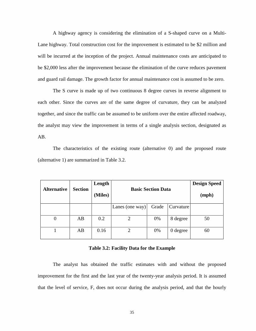
A highway agency is considering the elimination of a S-shaped curve on a Multi-
Lane highway. Total construction cost for the improvement is estimated to be $2 million and
will be incurred at the inception of the project. Annual maintenance costs are anticipated to
be $2,000 less after the improvement because the elimination of the curve reduces pavement
and guard rail damage. The growth factor for annual maintenance cost is assumed to be zero.
The S curve is made up of two continuous 8 degree curves in reverse alignment to
each other. Since the curves are of the same degree of curvature, they can be analyzed
together, and since the traffic can be assumed to be uniform over the entire affected roadway,
the analyst may view the improvement in terms of a single analysis section, designated as
AB.
The characteristics of the existing route (alternative 0) and the proposed route
(alternative 1) are summarized in Table 3.2.
Alternative SectionLength
(Miles)Basic Section Data
Design Speed
(mph)
Lanes (one way) Grade Curvature
0 AB 0.2 2 0% 8 degree 50
1 AB 0.16 2 0% 0 degree 60
Table 3.2: Facility Data for the Example
The analyst has obtained the traffic estimates with and without the proposed
improvement for the first and the last year of the twenty-year analysis period. It is assumed
that the level of service, F, does not occur during the analysis period, and that the hourly
36
variation of the traffic is small enough such that the explicit consideration of peaking
characteristics is unnecessary. Hence, the analysis is performed on an AADT basis. This
entails utilizing the traffic volume data for a typical hour of the day in each of the study
years. Such traffic data are summarized in Table 3.3, where a typical one way hourly volume
is defined as AADT divided by 18 (the number of hours assumed for a day). Note also that
capacity in year 20 is somewhat below that of year 1. This is to reflect normal deterioration
of the roadways over the years.
The traffic is assumed to be made of only passenger cars. The average running speed
is a function of the V/C ratio and other road characteristics and is computed from the
nomograph (Figure 3.1) and summarized in Table 3.3. Since speeds on the analysis section
will change as a result of the improvement, transition costs between sections will change;
thus speed on the previous section and the subsequent sections must be specified.
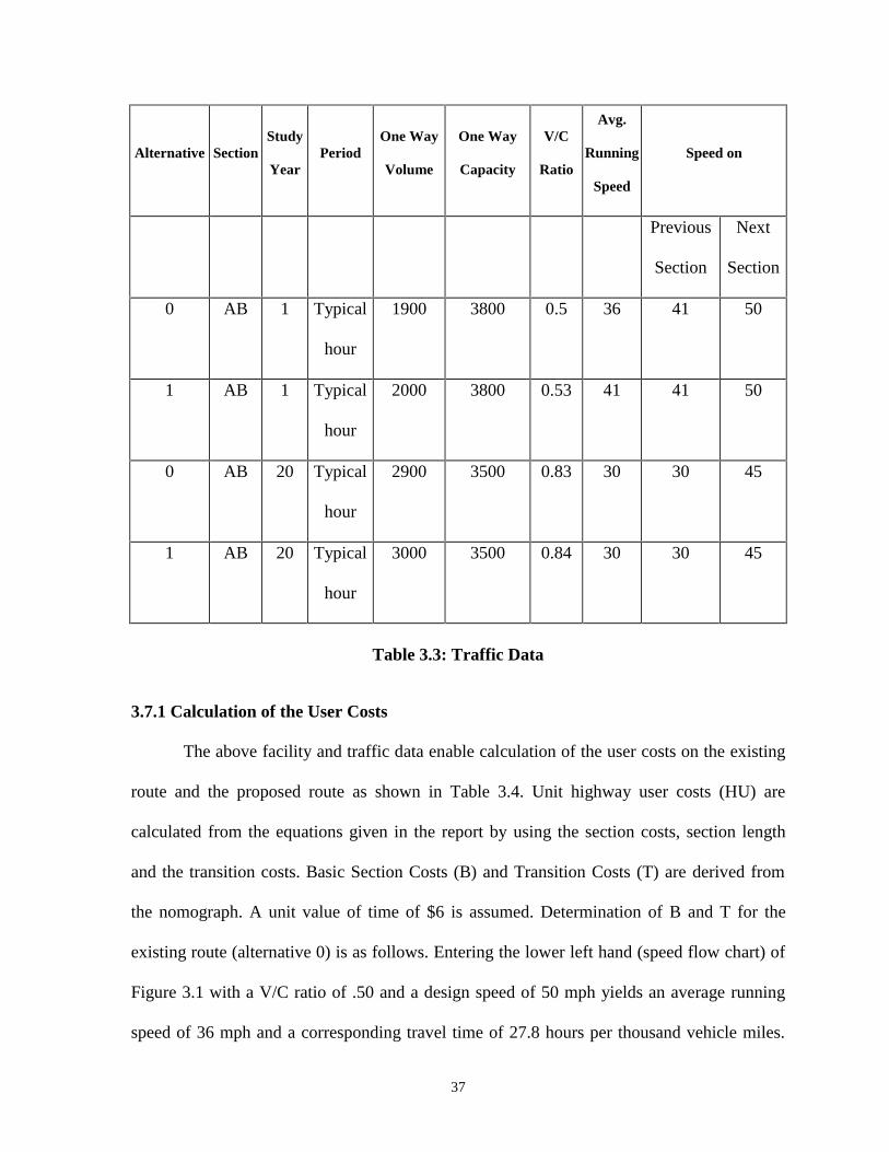
37
Alternative SectionStudy
YearPeriod
One Way
Volume
One Way
Capacity
V/C
Ratio
Avg.
Running
Speed
Speed on
Previous
Section
Next
Section
0 AB 1 Typical
hour
1900 3800 0.5 36 41 50
1 AB 1 Typical
hour
2000 3800 0.53 41 41 50
0 AB 20 Typical
hour
2900 3500 0.83 30 30 45
1 AB 20 Typical
hour
3000 3500 0.84 30 30 45
Table 3.3: Traffic Data
3.7.1 Calculation of the User Costs
The above facility and traffic data enable calculation of the user costs on the existing
route and the proposed route as shown in Table 3.4. Unit highway user costs (HU) are
calculated from the equations given in the report by using the section costs, section length
and the transition costs. Basic Section Costs (B) and Transition Costs (T) are derived from
the nomograph. A unit value of time of $6 is assumed. Determination of B and T for the
existing route (alternative 0) is as follows. Entering the lower left hand (speed flow chart) of
Figure 3.1 with a V/C ratio of .50 and a design speed of 50 mph yields an average running
speed of 36 mph and a corresponding travel time of 27.8 hours per thousand vehicle miles.
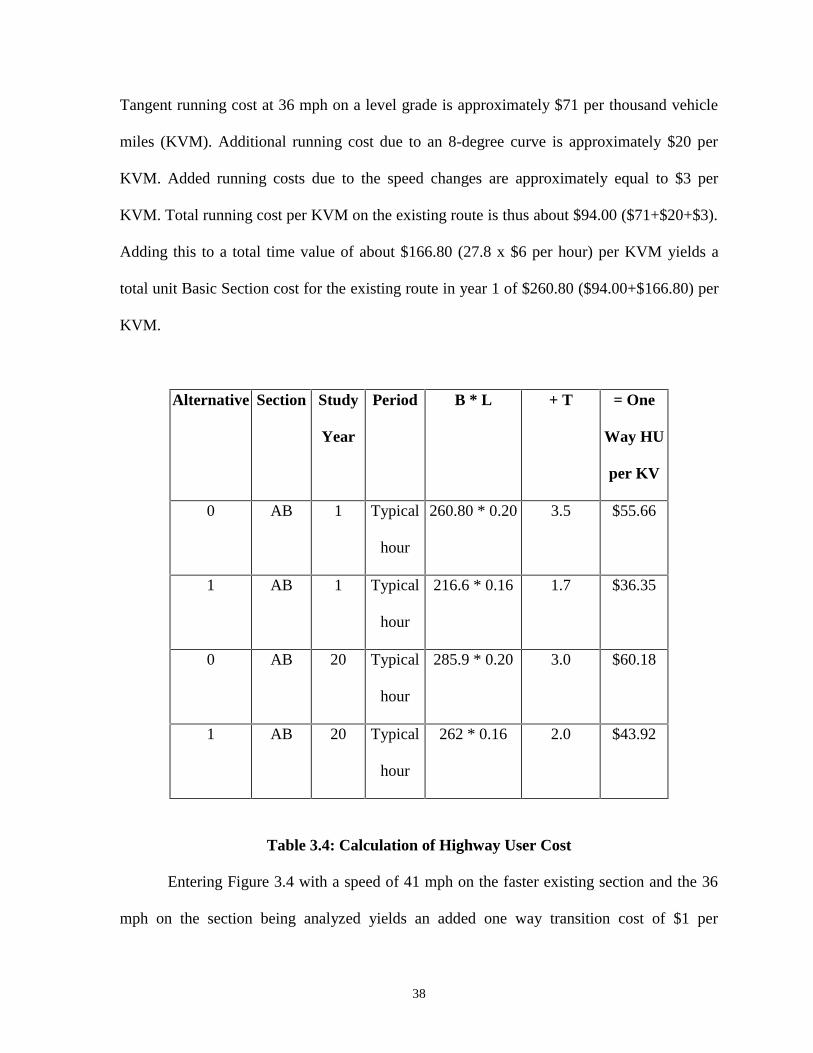
38
Tangent running cost at 36 mph on a level grade is approximately $71 per thousand vehicle
miles (KVM). Additional running cost due to an 8-degree curve is approximately $20 per
KVM. Added running costs due to the speed changes are approximately equal to $3 per
KVM. Total running cost per KVM on the existing route is thus about $94.00 ($71+$20+$3).
Adding this to a total time value of about $166.80 (27.8 x $6 per hour) per KVM yields a
total unit Basic Section cost for the existing route in year 1 of $260.80 ($94.00+$166.80) per
KVM.
Alternative Section Study
Year
Period B * L + T = One
Way HU
per KV
0 AB 1 Typical
hour
260.80 * 0.20 3.5 $55.66
1 AB 1 Typical
hour
216.6 * 0.16 1.7 $36.35
0 AB 20 Typical
hour
285.9 * 0.20 3.0 $60.18
1 AB 20 Typical
hour
262 * 0.16 2.0 $43.92
Table 3.4: Calculation of Highway User Cost
Entering Figure 3.4 with a speed of 41 mph on the faster existing section and the 36
mph on the section being analyzed yields an added one way transition cost of $1 per
39
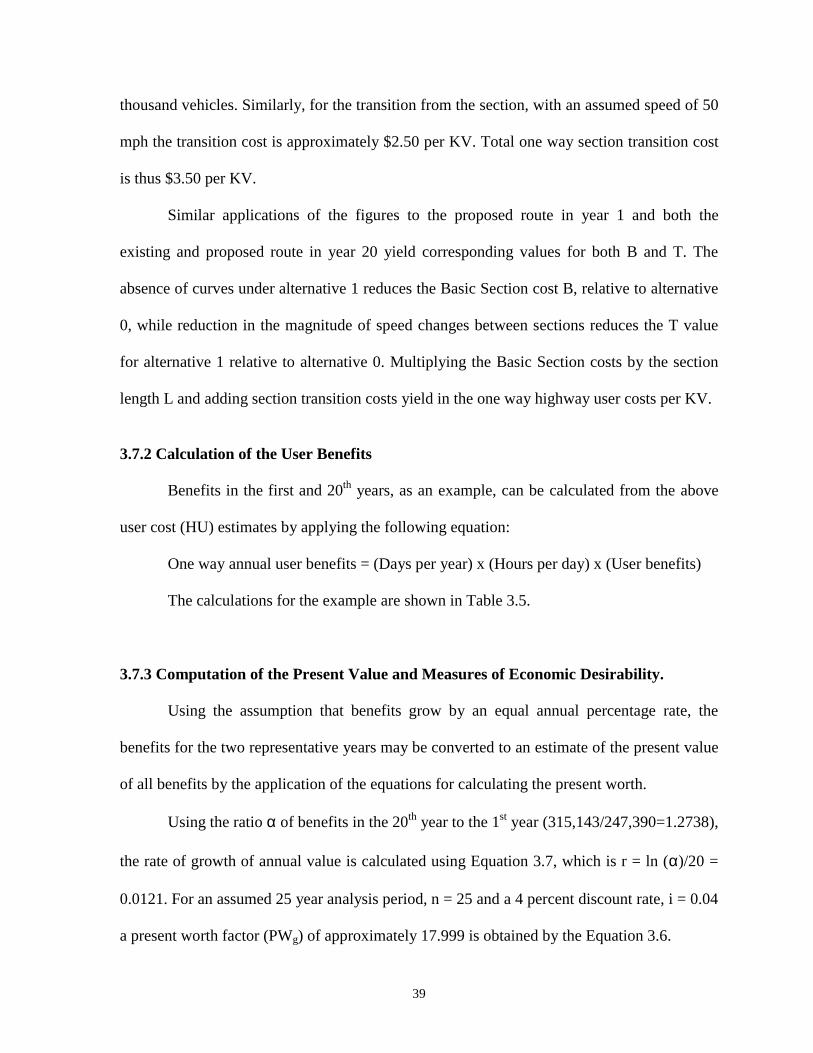
thousand vehicles. Similarly, for the transition from the section, with an assumed speed of 50
mph the transition cost is approximately $2.50 per KV. Total one way section transition cost
is thus $3.50 per KV.
Similar applications of the figures to the proposed route in year 1 and both the
existing and proposed route in year 20 yield corresponding values for both B and T. The
absence of curves under alternative 1 reduces the Basic Section cost B, relative to alternative
0, while reduction in the magnitude of speed changes between sections reduces the T value
for alternative 1 relative to alternative 0. Multiplying the Basic Section costs by the section
length L and adding section transition costs yield in the one way highway user costs per KV.
3.7.2 Calculation of the User Benefits
Benefits in the first and 20th years, as an example, can be calculated from the above
user cost (HU) estimates by applying the following equation:
One way annual user benefits = (Days per year) x (Hours per day) x (User benefits)
The calculations for the example are shown in Table 3.5.
3.7.3 Computation of the Present Value and Measures of Economic Desirability.
Using the assumption that benefits grow by an equal annual percentage rate, the
benefits for the two representative years may be converted to an estimate of the present value
of all benefits by the application of the equations for calculating the present worth.
Using the ratio α of benefits in the 20th year to the 1st year (315,143/247,390=1.2738),
the rate of growth of annual value is calculated using Equation 3.7, which is r = ln (α)/20 =
0.0121. For an assumed 25 year analysis period, n = 25 and a 4 percent discount rate, i = 0.04
a present worth factor (PWg) of approximately 17.999 is obtained by the Equation 3.6.
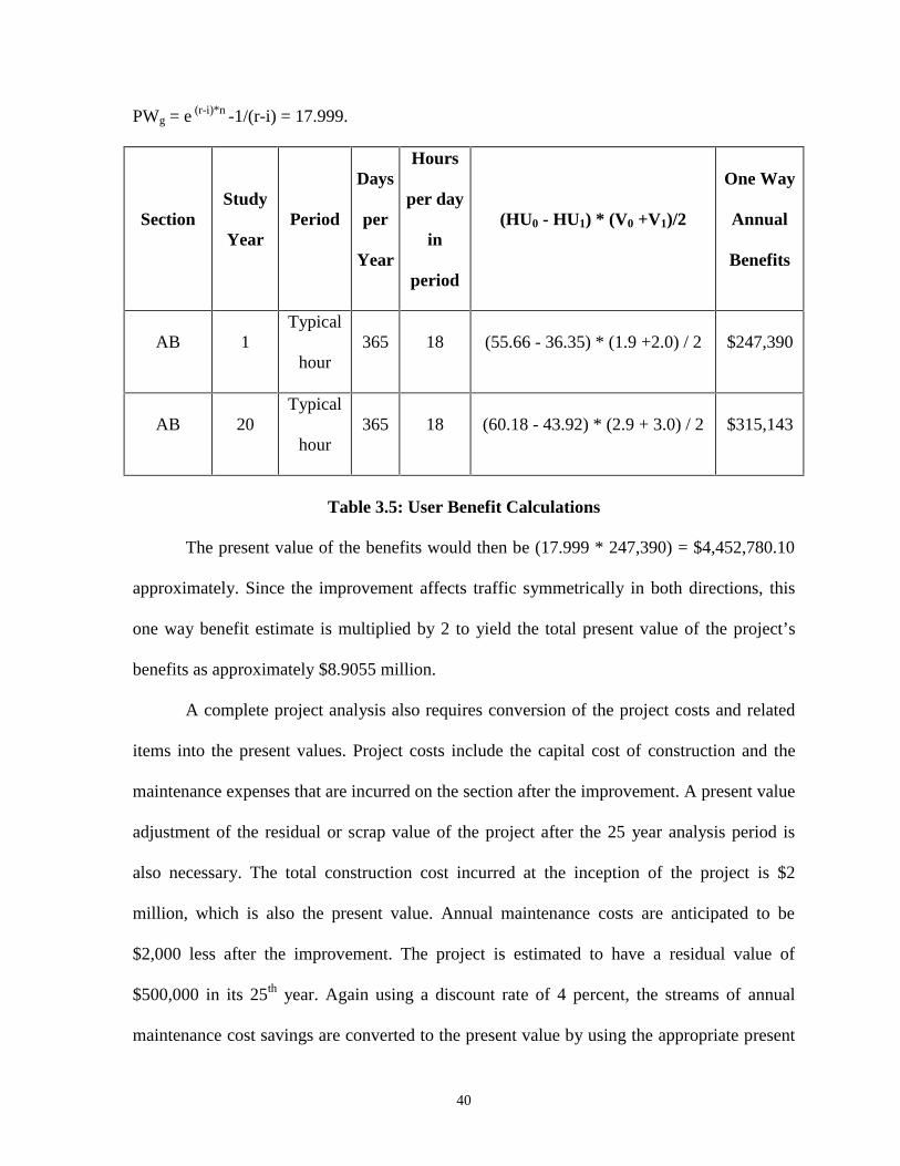
40
PWg = e (r-i)*n -1/(r-i) = 17.999.
SectionStudy
YearPeriod
Days
per
Year
Hours
per day
in
period
(HU0 - HU1) * (V0 +V1)/2
One Way
Annual
Benefits
AB 1Typical
hour365 18 (55.66 - 36.35) * (1.9 +2.0) / 2 $247,390
AB 20Typical
hour365 18 (60.18 - 43.92) * (2.9 + 3.0) / 2 $315,143
Table 3.5: User Benefit Calculations
The present value of the benefits would then be (17.999 * 247,390) = $4,452,780.10
approximately. Since the improvement affects traffic symmetrically in both directions, this
one way benefit estimate is multiplied by 2 to yield the total present value of the project’s
benefits as approximately $8.9055 million.
A complete project analysis also requires conversion of the project costs and related
items into the present values. Project costs include the capital cost of construction and the
maintenance expenses that are incurred on the section after the improvement. A present value
adjustment of the residual or scrap value of the project after the 25 year analysis period is
also necessary. The total construction cost incurred at the inception of the project is $2
million, which is also the present value. Annual maintenance costs are anticipated to be
$2,000 less after the improvement. The project is estimated to have a residual value of
$500,000 in its 25th year. Again using a discount rate of 4 percent, the streams of annual
maintenance cost savings are converted to the present value by using the appropriate present

41
worth series factor. The conversion of all projects related costs are summarized in the Table
3.6. The values 15.62 and 0.375 are the series present worth factor and the lumpsome present
worth factors, which gives the present worth of these values.
Item Value * Rate Present Value
Construction Cost $2,000,000 * 1.00 $2,000,000
Changes in Annual Maintenance Expenditure -$2,000 * 15.62 -$31,244
Residual Value in 25 Years -$500,000 * 0.375 -$187,558
Present Value of all Costs $1,781,198
Table 3.6: Calculation of Present Value of Project-Related Costs
The Net Present Value is the difference between the present values of the benefits and
the present values of the cost:
Net Present Value = Present Values of the Benefits - Present Value of the Costs
= $8,905,560 - $1,718,198
= $ 7,187,362
The Net Present Value of $7,187,362 indicates that the project is economically
desirable. The benefit cost ratio also suggests that the project is feasible because ($8,905,560)
/($2,000,000 - $31,244 - $187,558) or 4.99 is greater than 1.
However if there are budgetary constraints, the decision-maker should investigate
other projects or project alternatives for their relative economic attractiveness before making
a decision to implement the current project.
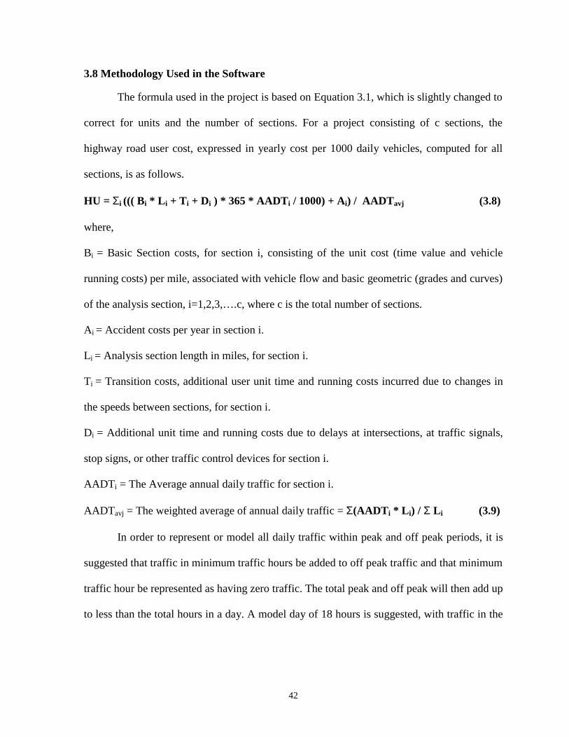
42
3.8 Methodology Used in the Software
The formula used in the project is based on Equation 3.1, which is slightly changed to
correct for units and the number of sections. For a project consisting of c sections, the
highway road user cost, expressed in yearly cost per 1000 daily vehicles, computed for all
sections, is as follows.
HU = Σi ((( Bi * Li + Ti + Di ) * 365 * AADTi / 1000) + Ai) / AADTavj (3.8)
where,
Bi = Basic Section costs, for section i, consisting of the unit cost (time value and vehicle
running costs) per mile, associated with vehicle flow and basic geometric (grades and curves)
of the analysis section, i=1,2,3,….c, where c is the total number of sections.
Ai = Accident costs per year in section i.
Li = Analysis section length in miles, for section i.
Ti = Transition costs, additional user unit time and running costs incurred due to changes in
the speeds between sections, for section i.
Di = Additional unit time and running costs due to delays at intersections, at traffic signals,
stop signs, or other traffic control devices for section i.
AADT i = The Average annual daily traffic for section i.
AADT avj = The weighted average of annual daily traffic = Σ(AADTi * Li) / Σ Li (3.9)
In order to represent or model all daily traffic within peak and off peak periods, it is
suggested that traffic in minimum traffic hours be added to off peak traffic and that minimum
traffic hour be represented as having zero traffic. The total peak and off peak will then add up
to less than the total hours in a day. A model day of 18 hours is suggested, with traffic in the
43
six hours from 12 midnight to 6 am added to off peak traffic. To compute the annualized
benefits for a project, a factor of 365 is applied to the unit daily cost.
The Basic Section cost is calculated in the same way as described in the 1977 Manual
(Section 3.2.1). The two methods in which accident cost is calculated are described in
Section 3.2.2. The first method is adopted in the software. The methods to calculate the
intersection delay costs and transition costs, respectively, are the same as those described in
Section 3.2.3 and Section 3.2.4 and have been adopted in the software without any changes.
The road user benefit is calculated by substituting in Equation 3.2 the value of HU for
old alternative and the new alternative calculated by Equation 3.7 and the AADTavj for the
old alternative and the new alternative calculated by Equation 3.9.
Thus, the formula is as follows:
User benefits = (HU0-HU1) [(AADTavj (0) +AADTavj (1))/2] (3.10)
The unit is in dollars per year. Among the various types of economic analysis that can
be performed to verify whether a project is desirable or not, the Net Present Value technique
as described in Section 3.5.2 has been used in the software. An example is provided in
Chapter 4 to illustrate the results produced by the software using the above methodology.
3.9 Cost Updating Procedures
It is noted that the nomographs shown in Figures 3.1 through 3.4 are based on
January 1975 price levels. It is recommended that the cost factors be reviewed and updated
once a year when the latest CPI’s become available. The 1977 Manual recommends a cost
updating procedure that employs multipliers based on commonly available consumer and
wholesale price indices published by the U.S. Bureau of Labor Statistics. It is noted that the
44
indices published in the 1977 Manual have been indexed to the period 1982-84 as a base unit
of 100.
Table 3.7 gives a list of consumer price indices and wholesale price indices (now
termed as wholesale price indices) updated to May 1997. The table also shows the January
1975 values as well as those values that have been adjusted for rebasing. These indices make
it possible to update the user costs from the nomographs for inflation.
A series of updating formulas was published in the 1977 Manual that accounts for the
various components of the user costs and recognizes that these components may escalate at
different rates. These formulas have been rearranged and shown in Tables 3.8(a) through
3.8(c). The formula provides a weighted average multiplier that accounts for the varying
rates of inflation. In the first formula in Table 3.8(a), for example, fuel costs accounted for 28
percent of total passenger car running costs on level tangents, motor oil accounts for 1
percent, tires account for 5 percent, and so on. In these formulas, for a given index variable,
Ri represent the ratio of the value of the present consumer price index to the adjusted value of
the January 1975 index and the subscript i denotes the component (f for fuel or fs for fuel,
single unit truck and so on).
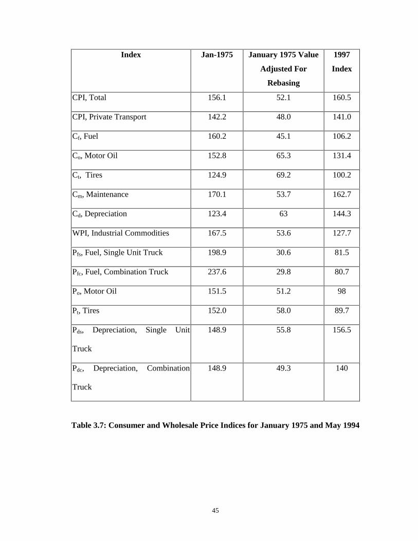
45
Index Jan-1975 January 1975 Value
Adjusted For
Rebasing
1997
Index
CPI, Total 156.1 52.1 160.5
CPI, Private Transport 142.2 48.0 141.0
Cf, Fuel 160.2 45.1 106.2
Co, Motor Oil 152.8 65.3 131.4
Ct, Tires 124.9 69.2 100.2
Cm, Maintenance 170.1 53.7 162.7
Cd, Depreciation 123.4 63 144.3
WPI, Industrial Commodities 167.5 53.6 127.7
Pfs, Fuel, Single Unit Truck 198.9 30.6 81.5
Pfc, Fuel, Combination Truck 237.6 29.8 80.7
Po, Motor Oil 151.5 51.2 98
Pt, Tires 152.0 58.0 89.7
Pds, Depreciation, Single Unit
Truck
148.9 55.8 156.5
Pdc, Depreciation, Combination
Truck
148.9 49.3 140
Table 3.7: Consumer and Wholesale Price Indices for January 1975 and May 1994
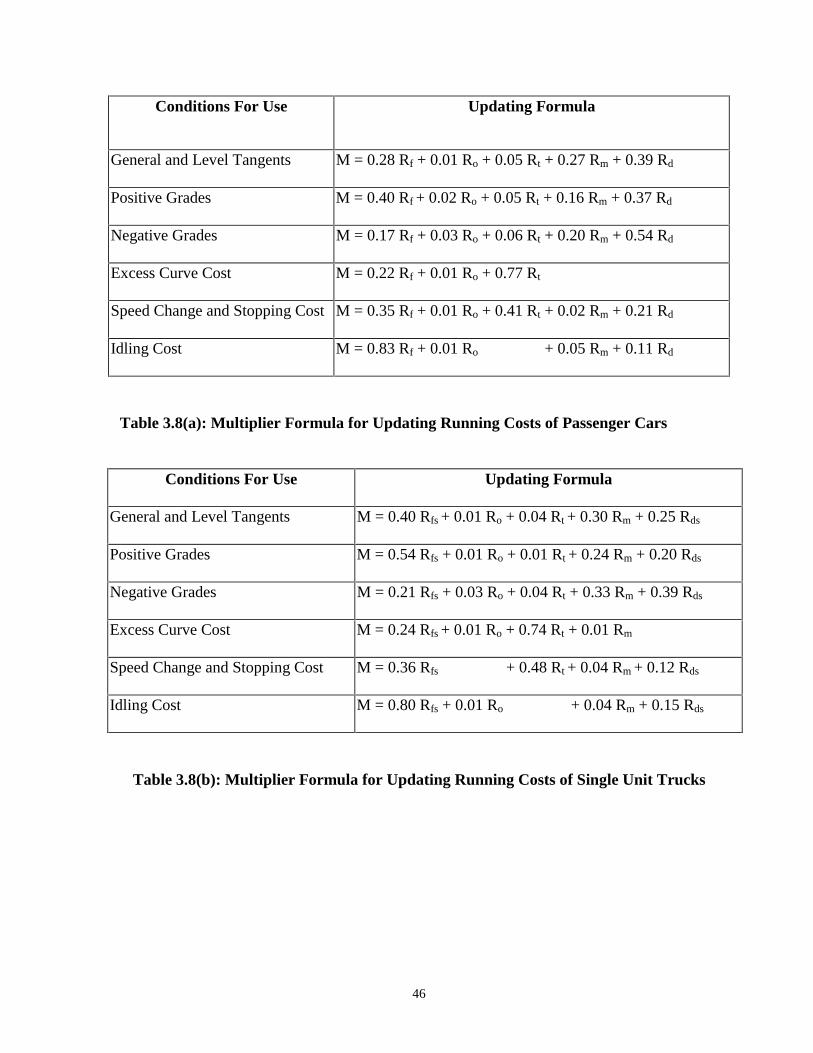
46
Conditions For Use Updating Formula
General and Level Tangents M = 0.28 Rf + 0.01 Ro + 0.05 Rt + 0.27 Rm + 0.39 Rd
Positive Grades M = 0.40 Rf + 0.02 Ro + 0.05 Rt + 0.16 Rm + 0.37 Rd
Negative Grades M = 0.17 Rf + 0.03 Ro + 0.06 Rt + 0.20 Rm + 0.54 Rd
Excess Curve Cost M = 0.22 Rf + 0.01 Ro + 0.77 Rt
Speed Change and Stopping Cost M = 0.35 Rf + 0.01 Ro + 0.41 Rt + 0.02 Rm + 0.21 Rd
Idling Cost M = 0.83 Rf + 0.01 Ro + 0.05 Rm + 0.11 Rd
Table 3.8(a): Multiplier Formula for Updating Running Costs of Passenger Cars
Conditions For Use Updating Formula
General and Level Tangents M = 0.40 Rfs + 0.01 Ro + 0.04 Rt + 0.30 Rm + 0.25 Rds
Positive Grades M = 0.54 Rfs + 0.01 Ro + 0.01 Rt + 0.24 Rm + 0.20 Rds
Negative Grades M = 0.21 Rfs + 0.03 Ro + 0.04 Rt + 0.33 Rm + 0.39 Rds
Excess Curve Cost M = 0.24 Rfs + 0.01 Ro + 0.74 Rt + 0.01 Rm
Speed Change and Stopping Cost M = 0.36 Rfs + 0.48 Rt + 0.04 Rm + 0.12 Rds
Idling Cost M = 0.80 Rfs + 0.01 Ro + 0.04 Rm + 0.15 Rds
Table 3.8(b): Multiplier Formula for Updating Running Costs of Single Unit Trucks
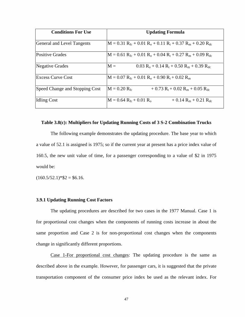
47
Conditions For Use Updating Formula
General and Level Tangents M = 0.31 Rfc + 0.01 Ro + 0.11 Rt + 0.37 Rm + 0.20 Rdc
Positive Grades M = 0.61 Rfc + 0.01 Ro + 0.04 Rt + 0.27 Rm + 0.09 Rdc
Negative Grades M = 0.03 Ro + 0.14 Rt + 0.50 Rm + 0.39 Rdc
Excess Curve Cost M = 0.07 Rfc + 0.01 Ro + 0.90 Rt + 0.02 Rm
Speed Change and Stopping Cost M = 0.20 Rfc + 0.73 Rt + 0.02 Rm + 0.05 Rdc
Idling Cost M = 0.64 Rfc + 0.01 Ro + 0.14 Rm + 0.21 Rdc
Table 3.8(c): Multipliers for Updating Running Costs of 3 S-2 Combination Trucks
The following example demonstrates the updating procedure. The base year to which
a value of 52.1 is assigned is 1975; so if the current year at present has a price index value of
160.5, the new unit value of time, for a passenger corresponding to a value of $2 in 1975
would be:
(160.5/52.1)*$2 = $6.16.
3.9.1 Updating Running Cost Factors
The updating procedures are described for two cases in the 1977 Manual. Case 1 is
for proportional cost changes when the components of running costs increase in about the
same proportion and Case 2 is for non-proportional cost changes when the components
change in significantly different proportions.
Case 1-For proportional cost changes: The updating procedure is the same as
described above in the example. However, for passenger cars, it is suggested that the private
transportation component of the consumer price index be used as the relevant index. For
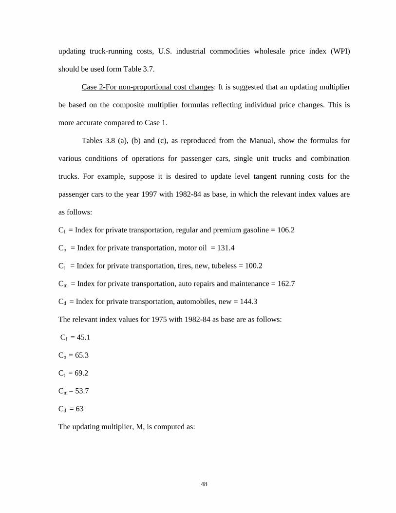
48
updating truck-running costs, U.S. industrial commodities wholesale price index (WPI)
should be used form Table 3.7.
Case 2-For non-proportional cost changes: It is suggested that an updating multiplier
be based on the composite multiplier formulas reflecting individual price changes. This is
more accurate compared to Case 1.
Tables 3.8 (a), (b) and (c), as reproduced from the Manual, show the formulas for
various conditions of operations for passenger cars, single unit trucks and combination
trucks. For example, suppose it is desired to update level tangent running costs for the
passenger cars to the year 1997 with 1982-84 as base, in which the relevant index values are
as follows:
Cf = Index for private transportation, regular and premium gasoline = 106.2
Co = Index for private transportation, motor oil = 131.4
Ct = Index for private transportation, tires, new, tubeless = 100.2
Cm = Index for private transportation, auto repairs and maintenance = 162.7
Cd = Index for private transportation, automobiles, new = 144.3
The relevant index values for 1975 with 1982-84 as base are as follows:
Cf = 45.1
Co = 65.3
Ct = 69.2
Cm = 53.7
Cd = 63
The updating multiplier, M, is computed as:
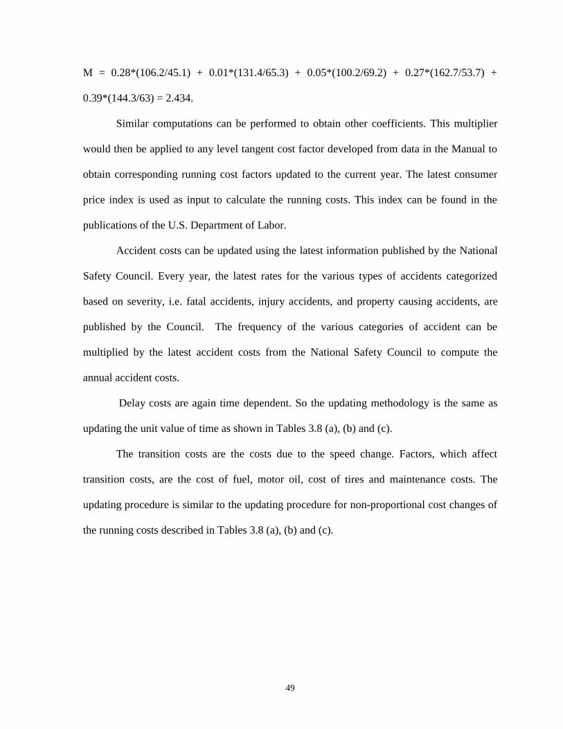
49
M = 0.28*(106.2/45.1) + 0.01*(131.4/65.3) + 0.05*(100.2/69.2) + 0.27*(162.7/53.7) +
0.39*(144.3/63) = 2.434.
Similar computations can be performed to obtain other coefficients. This multiplier
would then be applied to any level tangent cost factor developed from data in the Manual to
obtain corresponding running cost factors updated to the current year. The latest consumer
price index is used as input to calculate the running costs. This index can be found in the
publications of the U.S. Department of Labor.
Accident costs can be updated using the latest information published by the National
Safety Council. Every year, the latest rates for the various types of accidents categorized
based on severity, i.e. fatal accidents, injury accidents, and property causing accidents, are
published by the Council. The frequency of the various categories of accident can be
multiplied by the latest accident costs from the National Safety Council to compute the
annual accident costs.
Delay costs are again time dependent. So the updating methodology is the same as
updating the unit value of time as shown in Tables 3.8 (a), (b) and (c).
The transition costs are the costs due to the speed change. Factors, which affect
transition costs, are the cost of fuel, motor oil, cost of tires and maintenance costs. The
updating procedure is similar to the updating procedure for non-proportional cost changes of
the running costs described in Tables 3.8 (a), (b) and (c).
50
Chapter 4: Software Description and Usage
The software described in this report was developed to facilitate the use of the 1977
Manual. It performs all cost calculations stipulated in the Manual to compute road user cost
for a highway construction or improvement project. In addition, the software can be used to
perform Net Present Value analysis for a single project and comparison of various
alternatives. The software consists of the following two main modules:
1) User Cost-Benefit Application, and
2) Economic Analysis.
The first module is again divided into two sub-modules based on the type of the
operation carried out.
The first sub-module is designed to calculate the road user cost for the construction or
refurbishment of “uniform” highway sections. It is thus necessary to divide the project under
consideration into sections of reasonably similar geometric characteristics and traffic
conditions before using this module. This module is also used to update the road user cost
tables and forms the second sub-module.
The Economic Analysis module is designed to help determine whether a given project
or certain project alternatives can be deemed economically justifiable and to compare
different alternatives.
The first module is based on the methodology described in Chapter 3. This module
supply information needed for the second module to perform economic analysis and provide
economic justification of the project.

51
4.1 Software Development Tools
The software is built on an application development tool called Microsoft Visual
Basic 5. This means that, like other development tools such as Borland Delphi, Microsoft
Visual C++, and others, one can use Visual Basic 5 to construct software products that
solve specific problems. This tool is often called the front end because this is the software
that interacts with the user. As Microsoft’s premium programming language, Visual Basic 5
is the easiest object-oriented programming approach for application development. Microsoft
Visual Basic 5 is a sophisticated front end, which has some powerful features. The other
end is the backend, which the user does not interact with, but this is the part of the software
that interacts with the front end. Thus the front end has the unique ability of interacting with
both the user and the backend software. The back end for the software developed here is
Microsoft Excel, which is the data base handler. The database handler is the software where
the database resides. Both Visual Basic 5 and Microsoft Excel are products of Microsoft
making it both compatible and easily connected to each other. The Jet Database Engine is
used to establish such connection.
Visual Basic 5 has several outstanding features that have made it an efficient tool for
application development. It essentially consists of Forms or Screens, which are any normal
screen. In Visual Basic 5, the programmer builds the forms. These forms are similar to the
screens displayed by Windows 95 or Windows NT, such as logon dialog box shown at the
start up. The only difference is that the programmer decides get to choose how these dialog
boxes appear, when they appear, and what they do. Control Buttons or Toolbox Controls are
a set of controls that are used on the custom designed forms. Table 4.1 provides a set of
toolbox controls that have been used on the forms to arrive at the desired results in this

52
software. Control Buttons are located in the toolbox and are dragged with the help of the
mouse and placed on the screen or form. The positioning of these control buttons are often
specified by the software designer.
Control Use/Description
Text Box Displays and allows data entry.
LabelDisplays plain text on forms, such as captions for other
controls.
Combination Drop-downShows a current value selected from the list of possible
values
Command Button Initiates an action.
Option ButtonImplemented in groups, lets the user make a choice for a
small number of options.
FrameGroup controls that are related in some way; also displays
group of option buttons.
Table 4.1: Toolbox Controls Used in this Software
A number of other controls are also used. The controls are described individually in
the forms, where they are used. The Code Window, which is screened from the user, is the
driving force behind the software. Another property of Visual Basic 5 that was used in this
project is the Data Bound Controls. Bound Data Controls are the same as any other Visual
Basic 5 control objects, except that they may have been given additional properties, events,
and methods that allow the user to “bind” them directly to one or more data tables. The
binding makes it easy to create data-aware input and display objects that the user can user to
53
perform data input and display with little program code. The Data Control makes it easy to
write Visual Basic 5 programs that handle all of the following processes [Douglas, 1997]:
• Loading data from a database into a Visual Basic 5 Data object.
• Selecting the data records requested by the user.
• Loading form controls with the value of the requested records.
• Trapping simple user input errors.
• Enforcing database integrity rules.
• Updating the data object with modified data from the form control.
Visual Basic 5 Data Control is a control used to gain access to database tables. The Data
Control allows the user to establish a link to a single Dynaset Data object or Table or
Snapshot in a database. Basically, the Data Control is a link between the database and the
bound controls that the user uses to display the information. By default, the Data Control
creates a Dynaset-type recordset from one or more of the tables in the database. To perform
the linking to the MS-Excel sheets, the user has to select the Table-type recordset. The
recordset created by Data Control is determined by the settings of the DatabaseName and the
RecordSource properties. The recordset is created as the form containing the Data Control
loads and is activated. The recordset is active until the form is unloaded, at which the
recordset is released. This is the principle of database connectivity. It is possible to have
more than one Data Control on a single form.
The three main properties of Data Control that have been used are the DatabaseName
property, RecordSource Property and the Connect property. The DatabaseName property
contains the name of the database the user wants to access. The Connect property helps the
Jet Engine to know the type of database that is being connected at run time. MS-Excel has
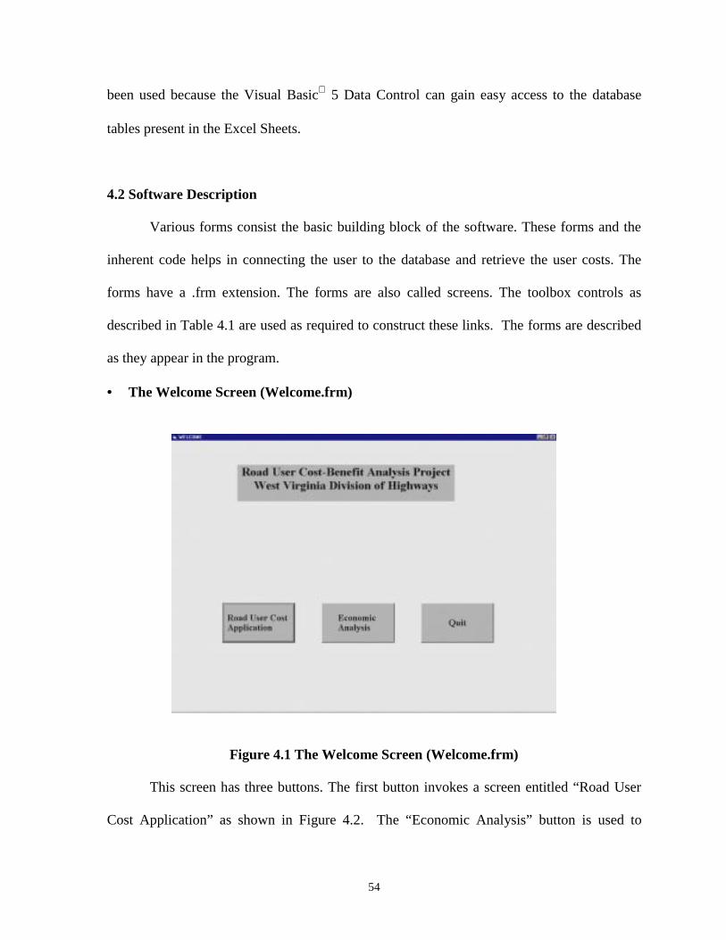
54
been used because the Visual Basic 5 Data Control can gain easy access to the database
tables present in the Excel Sheets.
4.2 Software Description
Various forms consist the basic building block of the software. These forms and the
inherent code helps in connecting the user to the database and retrieve the user costs. The
forms have a .frm extension. The forms are also called screens. The toolbox controls as
described in Table 4.1 are used as required to construct these links. The forms are described
as they appear in the program.
• The Welcome Screen (Welcome.frm)
Figure 4.1 The Welcome Screen (Welcome.frm)
This screen has three buttons. The first button invokes a screen entitled “Road User
Cost Application” as shown in Figure 4.2. The “Economic Analysis” button is used to
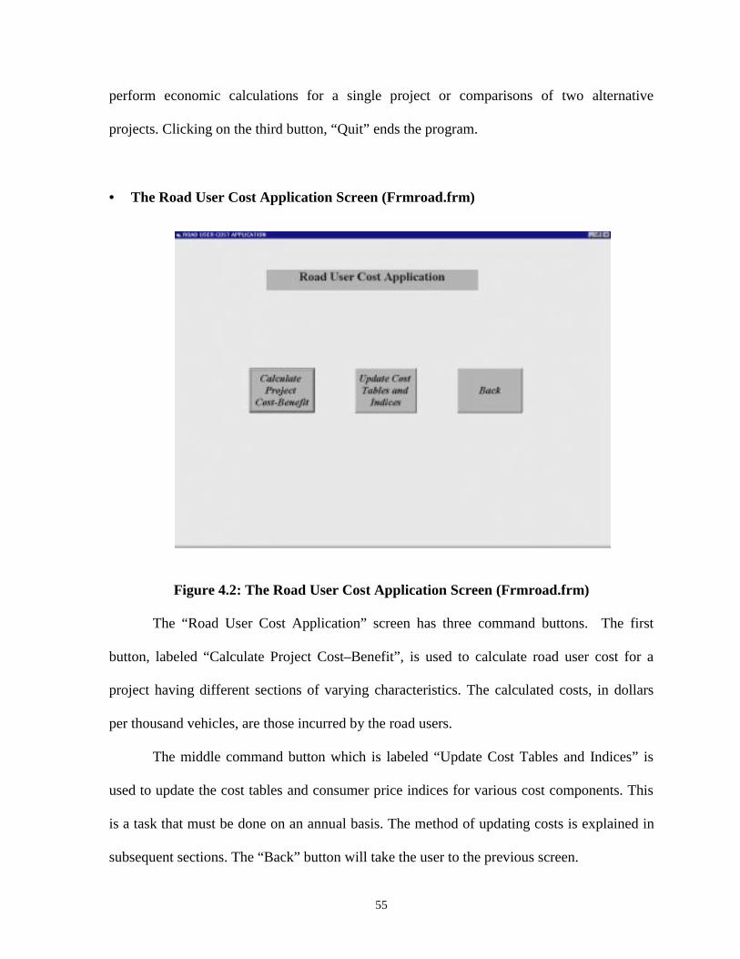
55
perform economic calculations for a single project or comparisons of two alternative
projects. Clicking on the third button, “Quit” ends the program.
• The Road User Cost Application Screen (Frmroad.frm)
Figure 4.2: The Road User Cost Application Screen (Frmroad.frm)
The “Road User Cost Application” screen has three command buttons. The first
button, labeled “Calculate Project Cost–Benefit”, is used to calculate road user cost for a
project having different sections of varying characteristics. The calculated costs, in dollars
per thousand vehicles, are those incurred by the road users.
The middle command button which is labeled “Update Cost Tables and Indices” is
used to update the cost tables and consumer price indices for various cost components. This
is a task that must be done on an annual basis. The method of updating costs is explained in
subsequent sections. The “Back” button will take the user to the previous screen.
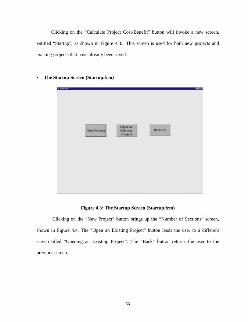
56
Clicking on the “Calculate Project Cost-Benefit” button will invoke a new screen,
entitled “Startup”, as shown in Figure 4.3. This screen is used for both new projects and
existing projects that have already been saved.
• The Startup Screen (Startup.frm)
Figure 4.3: The Startup Screen (Startup.frm)
Clicking on the “New Project” button brings up the “Number of Sections” screen,
shown in Figure 4.4. The “Open an Existing Project” button leads the user to a different
screen titled “Opening an Existing Project”. The “Back” button returns the user to the
previous screen.
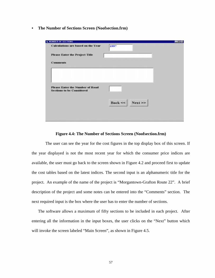
57
• The Number of Sections Screen (Noofsection.frm)
Figure 4.4: The Number of Sections Screen (Noofsection.frm)
The user can see the year for the cost figures in the top display box of this screen. If
the year displayed is not the most recent year for which the consumer price indices are
available, the user must go back to the screen shown in Figure 4.2 and proceed first to update
the cost tables based on the latest indices. The second input is an alphanumeric title for the
project. An example of the name of the project is “Morgantown-Grafton Route 22”. A brief
description of the project and some notes can be entered into the “Comments” section. The
next required input is the box where the user has to enter the number of sections.
The software allows a maximum of fifty sections to be included in each project. After
entering all the information in the input boxes, the user clicks on the “Next” button which
will invoke the screen labeled “Main Screen”, as shown in Figure 4.5.
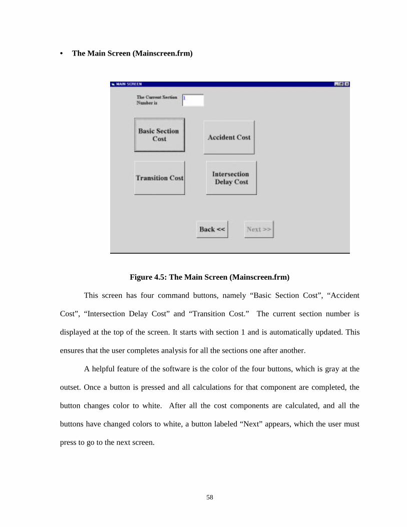
58
• The Main Screen (Mainscreen.frm)
Figure 4.5: The Main Screen (Mainscreen.frm)
This screen has four command buttons, namely “Basic Section Cost”, “Accident
Cost”, “Intersection Delay Cost” and “Transition Cost.” The current section number is
displayed at the top of the screen. It starts with section 1 and is automatically updated. This
ensures that the user completes analysis for all the sections one after another.
A helpful feature of the software is the color of the four buttons, which is gray at the
outset. Once a button is pressed and all calculations for that component are completed, the
button changes color to white. After all the cost components are calculated, and all the
buttons have changed colors to white, a button labeled “Next” appears, which the user must
press to go to the next screen.
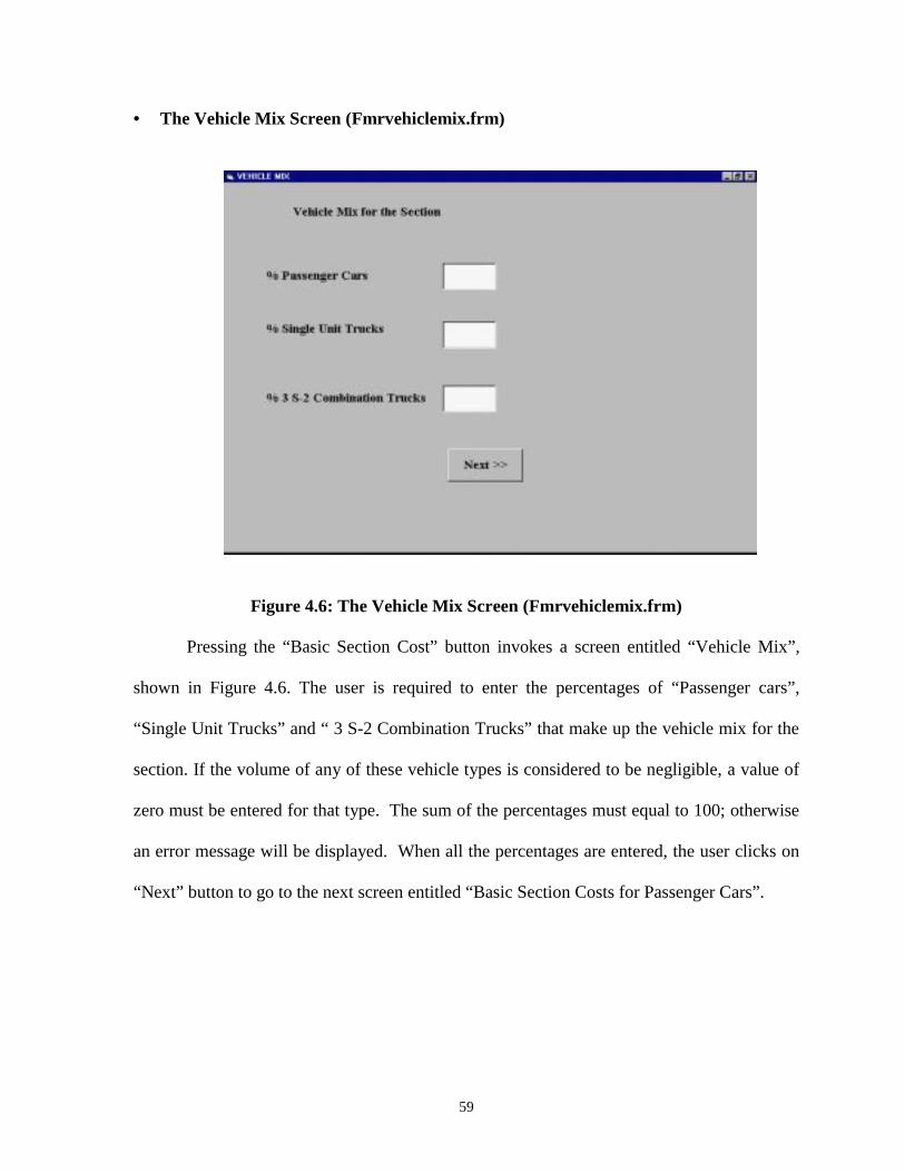
59
• The Vehicle Mix Screen (Fmrvehiclemix.frm)
Figure 4.6: The Vehicle Mix Screen (Fmrvehiclemix.frm)
Pressing the “Basic Section Cost” button invokes a screen entitled “Vehicle Mix”,
shown in Figure 4.6. The user is required to enter the percentages of “Passenger cars”,
“Single Unit Trucks” and “ 3 S-2 Combination Trucks” that make up the vehicle mix for the
section. If the volume of any of these vehicle types is considered to be negligible, a value of
zero must be entered for that type. The sum of the percentages must equal to 100; otherwise
an error message will be displayed. When all the percentages are entered, the user clicks on
“Next” button to go to the next screen entitled “Basic Section Costs for Passenger Cars”.
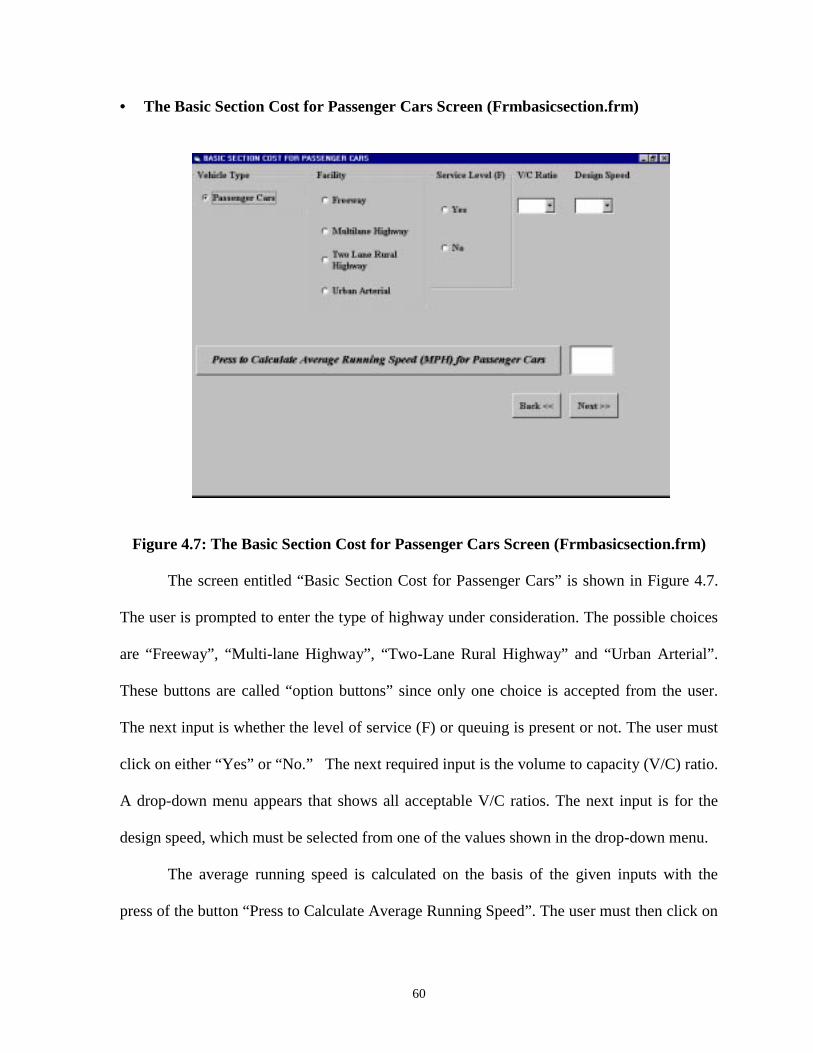
60
• The Basic Section Cost for Passenger Cars Screen (Frmbasicsection.frm)
Figure 4.7: The Basic Section Cost for Passenger Cars Screen (Frmbasicsection.frm)
The screen entitled “Basic Section Cost for Passenger Cars” is shown in Figure 4.7.
The user is prompted to enter the type of highway under consideration. The possible choices
are “Freeway”, “Multi-lane Highway”, “Two-Lane Rural Highway” and “Urban Arterial”.
These buttons are called “option buttons” since only one choice is accepted from the user.
The next input is whether the level of service (F) or queuing is present or not. The user must
click on either “Yes” or “No.” The next required input is the volume to capacity (V/C) ratio.
A drop-down menu appears that shows all acceptable V/C ratios. The next input is for the
design speed, which must be selected from one of the values shown in the drop-down menu.
The average running speed is calculated on the basis of the given inputs with the
press of the button “Press to Calculate Average Running Speed”. The user must then click on
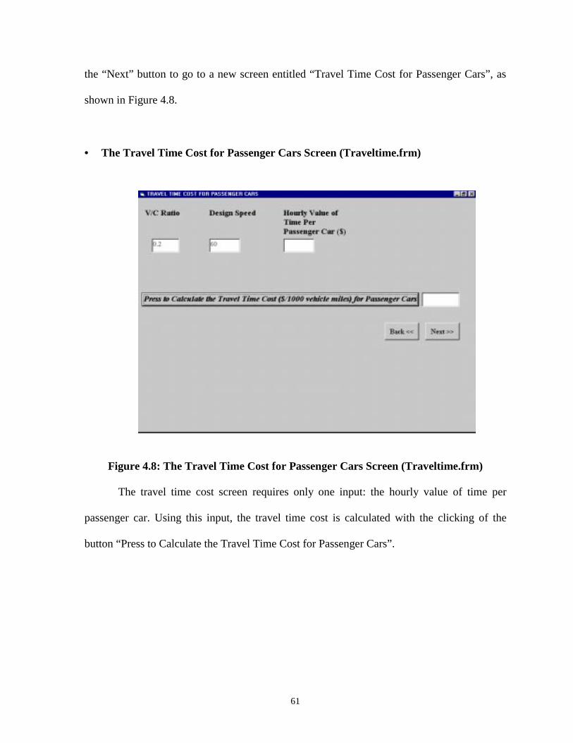
61
the “Next” button to go to a new screen entitled “Travel Time Cost for Passenger Cars”, as
shown in Figure 4.8.
• The Travel Time Cost for Passenger Cars Screen (Traveltime.frm)
Figure 4.8: The Travel Time Cost for Passenger Cars Screen (Traveltime.frm)
The travel time cost screen requires only one input: the hourly value of time per
passenger car. Using this input, the travel time cost is calculated with the clicking of the
button “Press to Calculate the Travel Time Cost for Passenger Cars”.
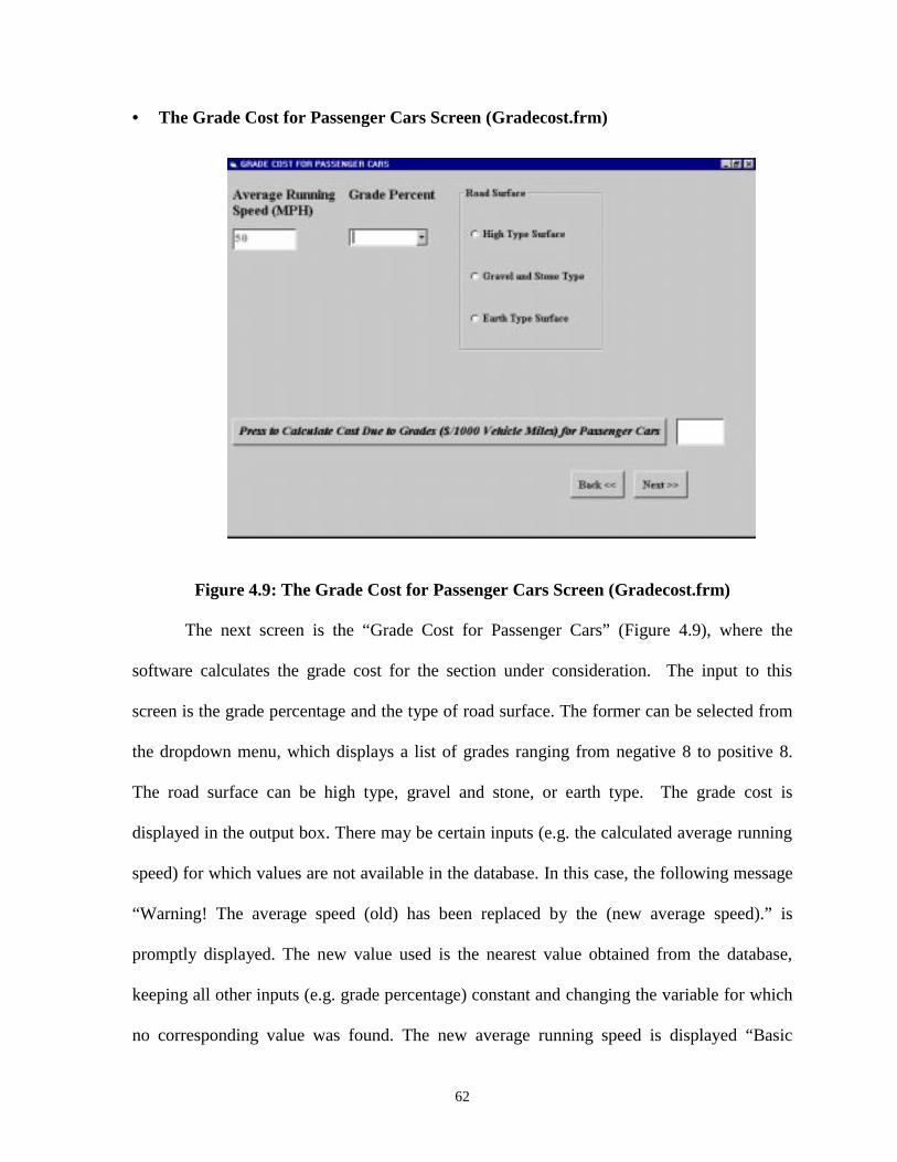
62
• The Grade Cost for Passenger Cars Screen (Gradecost.frm)
Figure 4.9: The Grade Cost for Passenger Cars Screen (Gradecost.frm)
The next screen is the “Grade Cost for Passenger Cars” (Figure 4.9), where the
software calculates the grade cost for the section under consideration. The input to this
screen is the grade percentage and the type of road surface. The former can be selected from
the dropdown menu, which displays a list of grades ranging from negative 8 to positive 8.
The road surface can be high type, gravel and stone, or earth type. The grade cost is
displayed in the output box. There may be certain inputs (e.g. the calculated average running
speed) for which values are not available in the database. In this case, the following message
“Warning! The average speed (old) has been replaced by the (new average speed).” is
promptly displayed. The new value used is the nearest value obtained from the database,
keeping all other inputs (e.g. grade percentage) constant and changing the variable for which
no corresponding value was found. The new average running speed is displayed “Basic
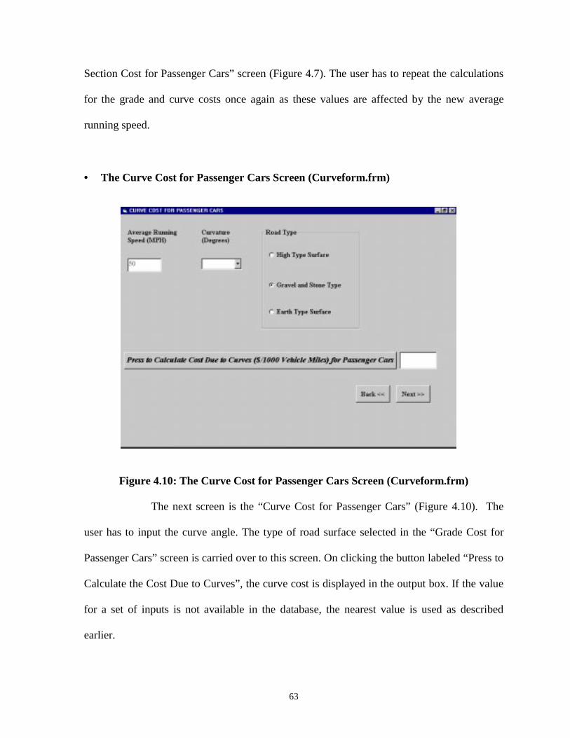
63
Section Cost for Passenger Cars” screen (Figure 4.7). The user has to repeat the calculations
for the grade and curve costs once again as these values are affected by the new average
running speed.
• The Curve Cost for Passenger Cars Screen (Curveform.frm)
Figure 4.10: The Curve Cost for Passenger Cars Screen (Curveform.frm)
The next screen is the “Curve Cost for Passenger Cars” (Figure 4.10). The
user has to input the curve angle. The type of road surface selected in the “Grade Cost for
Passenger Cars” screen is carried over to this screen. On clicking the button labeled “Press to
Calculate the Cost Due to Curves”, the curve cost is displayed in the output box. If the value
for a set of inputs is not available in the database, the nearest value is used as described
earlier.
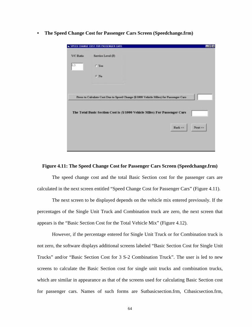
64
• The Speed Change Cost for Passenger Cars Screen (Speedchange.frm)
Figure 4.11: The Speed Change Cost for Passenger Cars Screen (Speedchange.frm)
The speed change cost and the total Basic Section cost for the passenger cars are
calculated in the next screen entitled “Speed Change Cost for Passenger Cars” (Figure 4.11).
The next screen to be displayed depends on the vehicle mix entered previously. If the
percentages of the Single Unit Truck and Combination truck are zero, the next screen that
appears is the “Basic Section Cost for the Total Vehicle Mix” (Figure 4.12).
However, if the percentage entered for Single Unit Truck or for Combination truck is
not zero, the software displays additional screens labeled “Basic Section Cost for Single Unit
Trucks” and/or “Basic Section Cost for 3 S-2 Combination Truck”. The user is led to new
screens to calculate the Basic Section cost for single unit trucks and combination trucks,
which are similar in appearance as that of the screens used for calculating Basic Section cost
for passenger cars. Names of such forms are Sutbasicsection.frm, Ctbasicsection.frm,
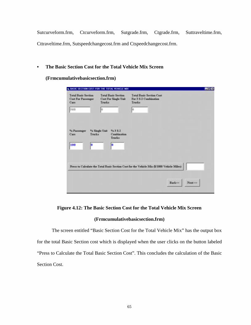
65
Sutcurveform.frm, Ctcurveform.frm, Sutgrade.frm, Ctgrade.frm, Suttraveltime.frm,
Cttraveltime.frm, Sutspeedchangecost.frm and Ctspeedchangecost.frm.
• The Basic Section Cost for the Total Vehicle Mix Screen
(Frmcumulativebasicsection.frm)
Figure 4.12: The Basic Section Cost for the Total Vehicle Mix Screen
(Frmcumulativebasicsection.frm)
The screen entitled “Basic Section Cost for the Total Vehicle Mix” has the output box
for the total Basic Section cost which is displayed when the user clicks on the button labeled
“Press to Calculate the Total Basic Section Cost”. This concludes the calculation of the Basic
Section Cost.
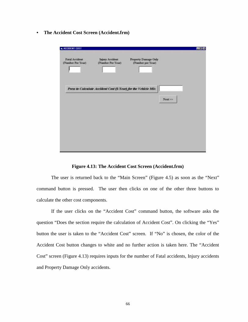
66
• The Accident Cost Screen (Accident.frm)
Figure 4.13: The Accident Cost Screen (Accident.frm)
The user is returned back to the “Main Screen” (Figure 4.5) as soon as the “Next”
command button is pressed. The user then clicks on one of the other three buttons to
calculate the other cost components.
If the user clicks on the “Accident Cost” command button, the software asks the
question “Does the section require the calculation of Accident Cost”. On clicking the “Yes”
button the user is taken to the “Accident Cost” screen. If “No” is chosen, the color of the
Accident Cost button changes to white and no further action is taken here. The “Accident
Cost” screen (Figure 4.13) requires inputs for the number of Fatal accidents, Injury accidents
and Property Damage Only accidents.
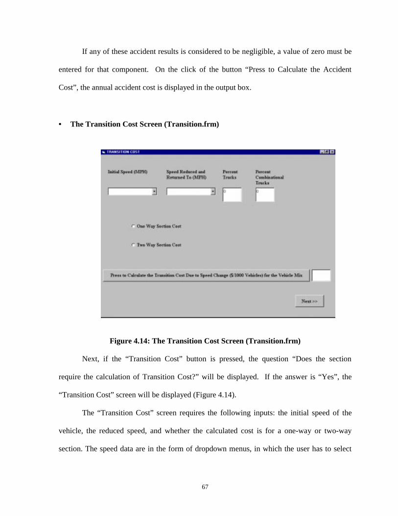
67
If any of these accident results is considered to be negligible, a value of zero must be
entered for that component. On the click of the button “Press to Calculate the Accident
Cost”, the annual accident cost is displayed in the output box.
• The Transition Cost Screen (Transition.frm)
Figure 4.14: The Transition Cost Screen (Transition.frm)
Next, if the “Transition Cost” button is pressed, the question “Does the section
require the calculation of Transition Cost?” will be displayed. If the answer is “Yes”, the
“Transition Cost” screen will be displayed (Figure 4.14).
The “Transition Cost” screen requires the following inputs: the initial speed of the
vehicle, the reduced speed, and whether the calculated cost is for a one-way or two-way
section. The speed data are in the form of dropdown menus, in which the user has to select

68
from a list and the number of ways is in the form of an option button. On clicking the button
“Press to Calculate the Transition Cost”, the transition cost is displayed in the output box.
The “Next” button takes the user back to the “Main Screen”.
• The Intersection Delay Cost Due to Stopping Screen (Delaycosts.frm)
Figure 4.15: The Intersection Delay Cost Due to Stopping Screen (Delaycosts.frm)
The final cost component to be calculated is the intersection delay cost. If the user
chooses to include the delay cost in the calculations, the “Delay Cost” screen (Figure 4.15)
will be displayed. To calculate the Delay Cost, the following inputs are required: “Traffic
Volume”, “Road Capacity”, “Signal Cycle Time (Seconds)”, “Effective Green Time
(Seconds)”, “Intersection Approach Speed”. “Hourly Value of Time for Passenger Cars”,
“Percent Single Unit Trucks” and “Percent Combination Trucks” are the inputs already
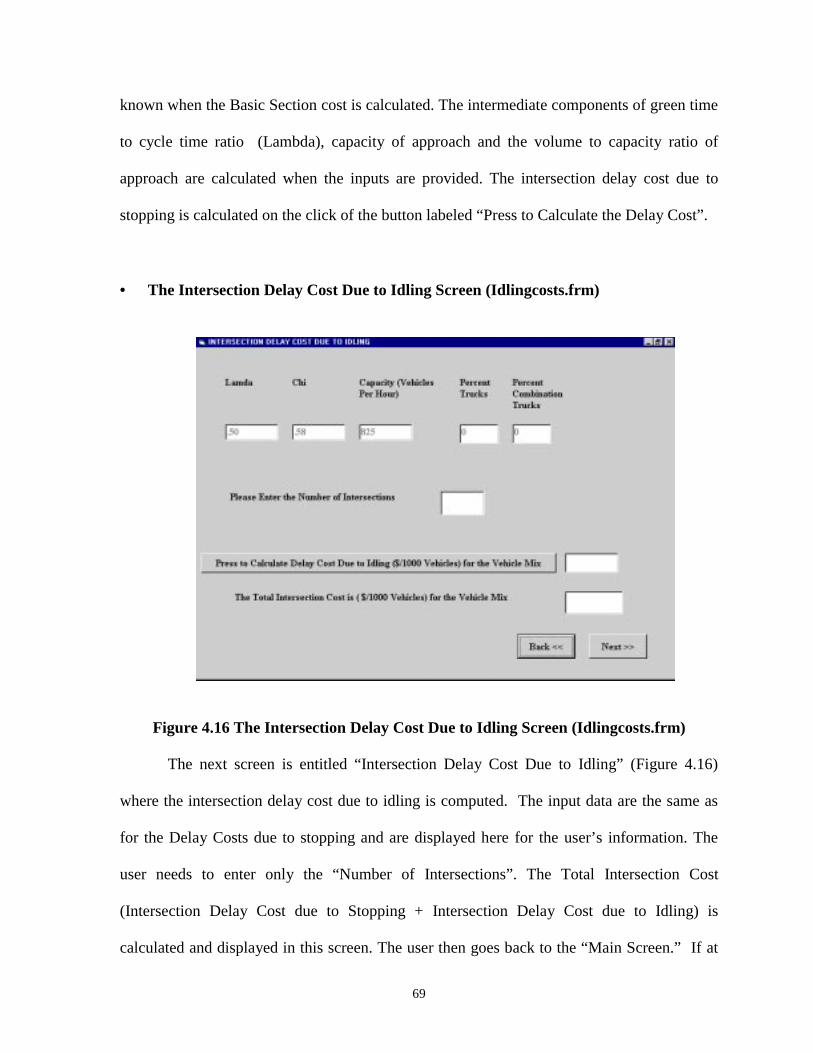
69
known when the Basic Section cost is calculated. The intermediate components of green time
to cycle time ratio (Lambda), capacity of approach and the volume to capacity ratio of
approach are calculated when the inputs are provided. The intersection delay cost due to
stopping is calculated on the click of the button labeled “Press to Calculate the Delay Cost”.
• The Intersection Delay Cost Due to Idling Screen (Idlingcosts.frm)
Figure 4.16 The Intersection Delay Cost Due to Idling Screen (Idlingcosts.frm)
The next screen is entitled “Intersection Delay Cost Due to Idling” (Figure 4.16)
where the intersection delay cost due to idling is computed. The input data are the same as
for the Delay Costs due to stopping and are displayed here for the user’s information. The
user needs to enter only the “Number of Intersections”. The Total Intersection Cost
(Intersection Delay Cost due to Stopping + Intersection Delay Cost due to Idling) is
calculated and displayed in this screen. The user then goes back to the “Main Screen.” If at
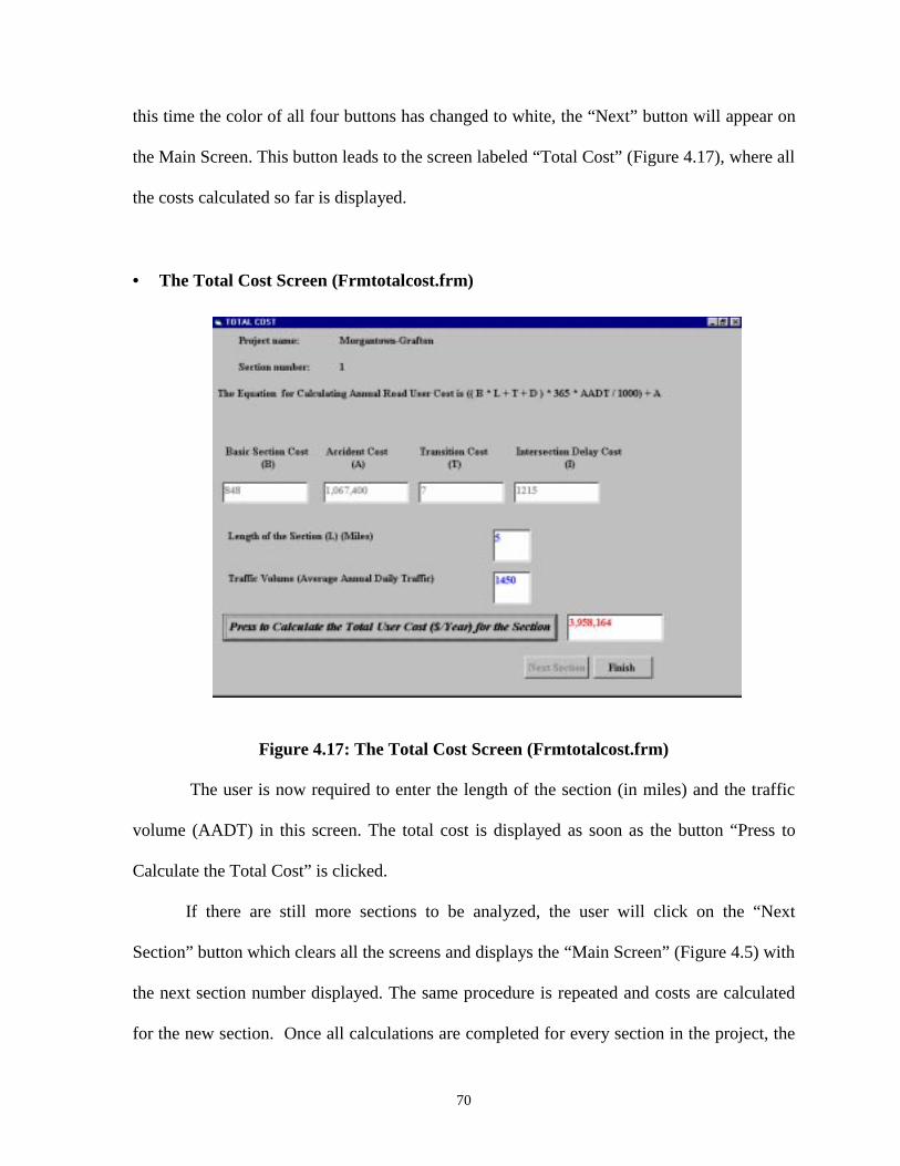
70
this time the color of all four buttons has changed to white, the “Next” button will appear on
the Main Screen. This button leads to the screen labeled “Total Cost” (Figure 4.17), where all
the costs calculated so far is displayed.
• The Total Cost Screen (Frmtotalcost.frm)
Figure 4.17: The Total Cost Screen (Frmtotalcost.frm)
The user is now required to enter the length of the section (in miles) and the traffic
volume (AADT) in this screen. The total cost is displayed as soon as the button “Press to
Calculate the Total Cost” is clicked.
If there are still more sections to be analyzed, the user will click on the “Next
Section” button which clears all the screens and displays the “Main Screen” (Figure 4.5) with
the next section number displayed. The same procedure is repeated and costs are calculated
for the new section. Once all calculations are completed for every section in the project, the
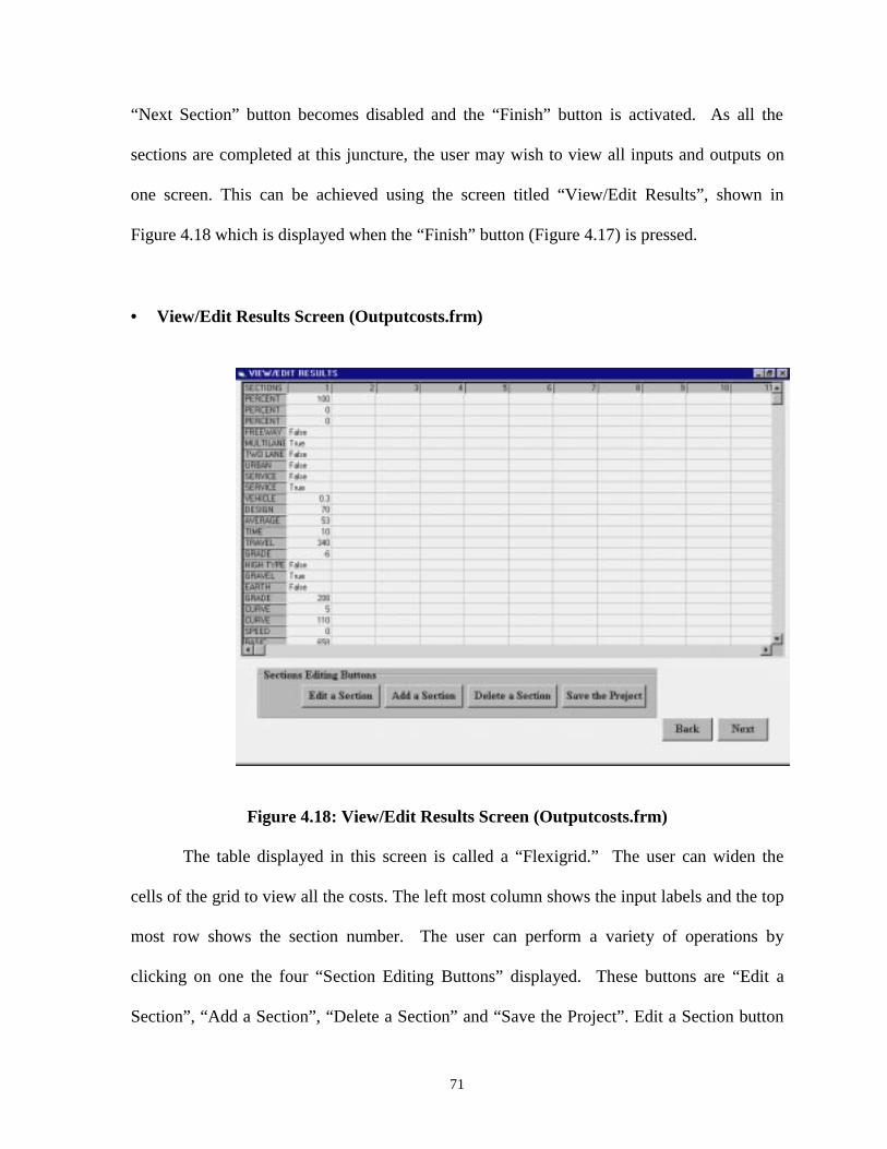
71
“Next Section” button becomes disabled and the “Finish” button is activated. As all the
sections are completed at this juncture, the user may wish to view all inputs and outputs on
one screen. This can be achieved using the screen titled “View/Edit Results”, shown in
Figure 4.18 which is displayed when the “Finish” button (Figure 4.17) is pressed.
• View/Edit Results Screen (Outputcosts.frm)
Figure 4.18: View/Edit Results Screen (Outputcosts.frm)
The table displayed in this screen is called a “Flexigrid.” The user can widen the
cells of the grid to view all the costs. The left most column shows the input labels and the top
most row shows the section number. The user can perform a variety of operations by
clicking on one the four “Section Editing Buttons” displayed. These buttons are “Edit a
Section”, “Add a Section”, “Delete a Section” and “Save the Project”. Edit a Section button
72
is used to make modifications in a particular section. If the user clicks on this button, an input
box will be displayed prompting the user for the section number to be edited, after which the
“Main Screen” will be displayed. All calculations for that section can be repeated with the
modified inputs.
If it is desired to add a new section to the project, clicking on the “Add a Section”
button will take the user back to the “Main Screen”. The number of sections in the project
will be increased by one. However, if there are already 50 sections in the project, no more
sections can be added. Attempts to increase the number of sections above 50 will result in an
error message.
The “Delete a Section” button is useful if the user is no longer interested in a
particular section and wants to remove it from the project. An input box will be displayed
asking the user to enter the section number to be deleted. Once the section number is entered,
it is automatically deleted from the project. Multiple sections can be deleted one by one.
Once the user is fully satisfied with the results, “Save the Project” button must be
pressed. A window, as shown in Figure 4.19, will be displayed and the “View/Edit Results”
screen will be disabled. The user has to press the “Save” button to save the project in a
desired directory. The project is then saved in an ASCII text file in the harddrive (C:\) for
future retrieval and the “View/Edit Results” screen is enabled once more. A message entitled
“If you have not saved the file, Please do so” is displayed as soon as the “Next” button is
pressed. It is the responsibility of the user to save the file in the desired directory. If the
project is not saved at this juncture, the user may lose all information. On pressing the “Ok”
button of the message box, the next screen titled “Inputs for the Project” screen (Figure 4.20)
is displayed.
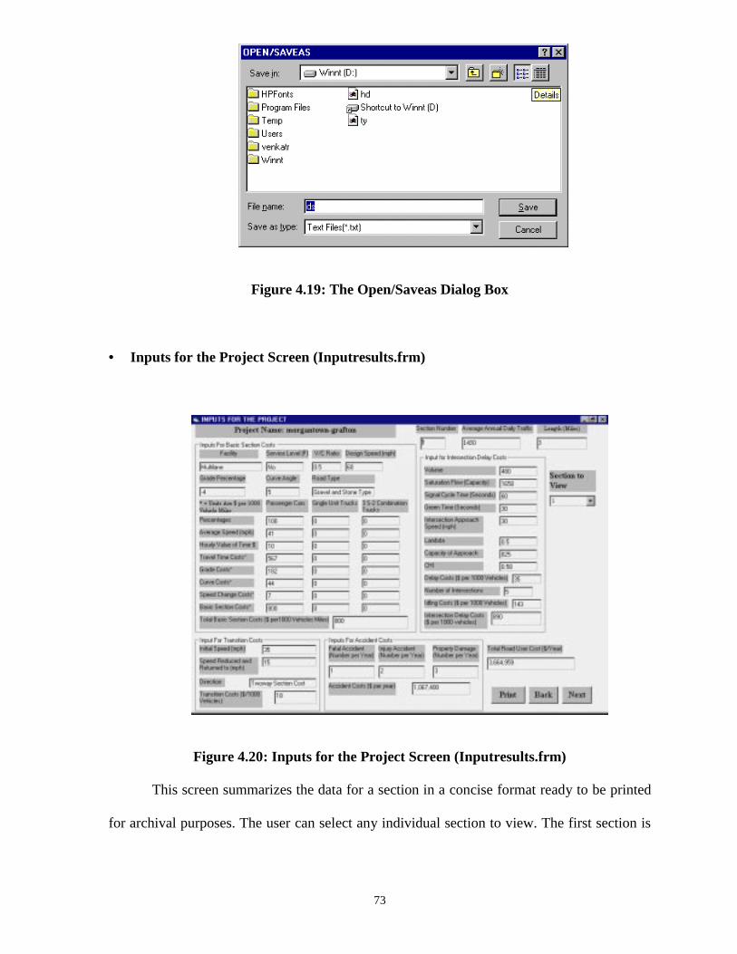
73
Figure 4.19: The Open/Saveas Dialog Box
• Inputs for the Project Screen (Inputresults.frm)
Figure 4.20: Inputs for the Project Screen (Inputresults.frm)
This screen summarizes the data for a section in a concise format ready to be printed
for archival purposes. The user can select any individual section to view. The first section is
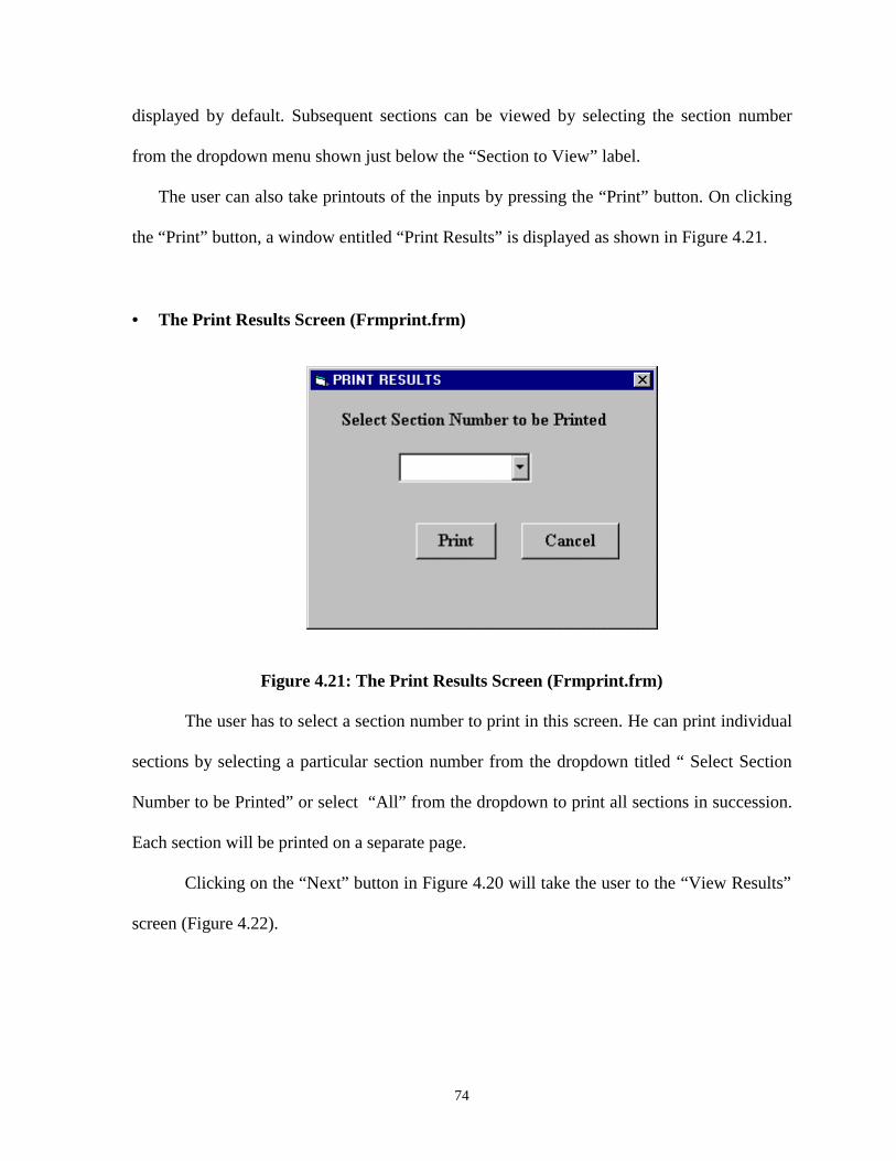
74
displayed by default. Subsequent sections can be viewed by selecting the section number
from the dropdown menu shown just below the “Section to View” label.
The user can also take printouts of the inputs by pressing the “Print” button. On clicking
the “Print” button, a window entitled “Print Results” is displayed as shown in Figure 4.21.
• The Print Results Screen (Frmprint.frm)
Figure 4.21: The Print Results Screen (Frmprint.frm)
The user has to select a section number to print in this screen. He can print individual
sections by selecting a particular section number from the dropdown titled “ Select Section
Number to be Printed” or select “All” from the dropdown to print all sections in succession.
Each section will be printed on a separate page.
Clicking on the “Next” button in Figure 4.20 will take the user to the “View Results”
screen (Figure 4.22).
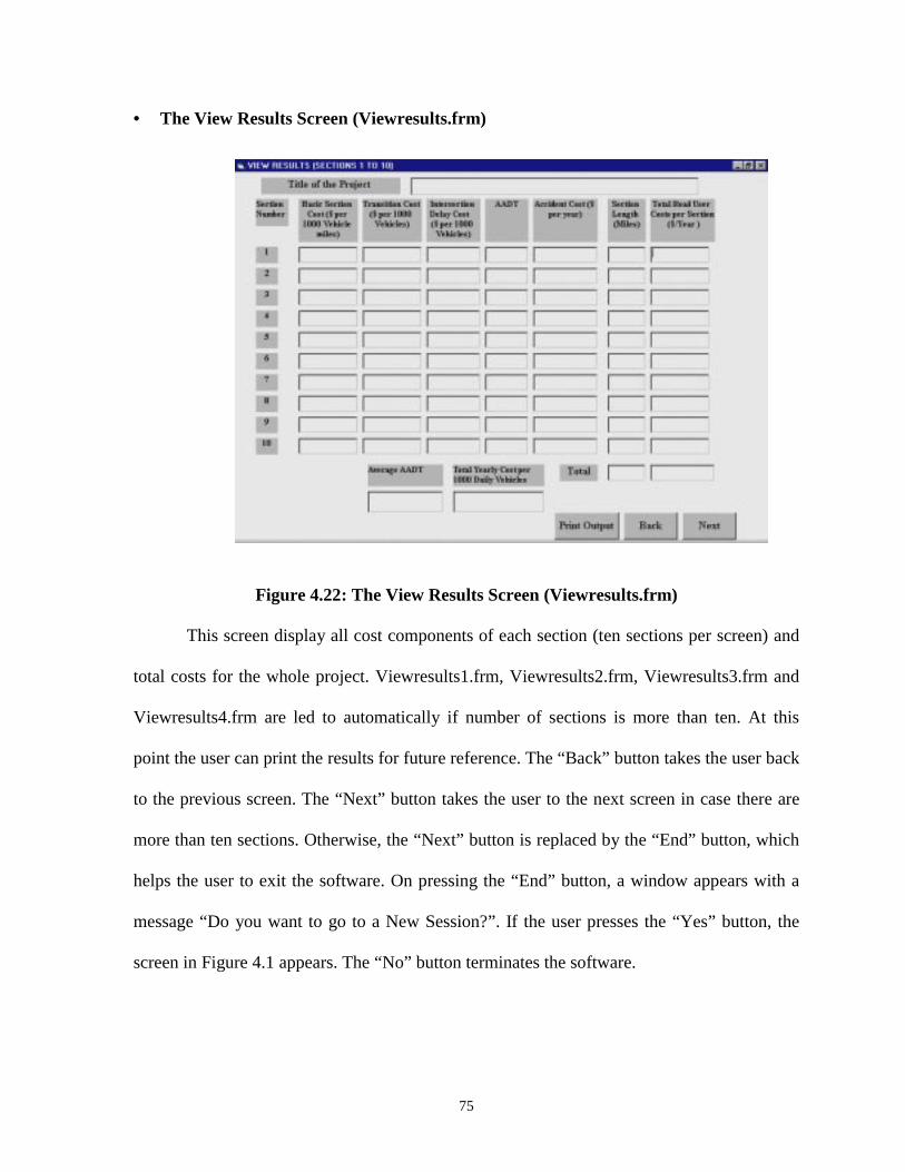
75
• The View Results Screen (Viewresults.frm)
Figure 4.22: The View Results Screen (Viewresults.frm)
This screen display all cost components of each section (ten sections per screen) and
total costs for the whole project. Viewresults1.frm, Viewresults2.frm, Viewresults3.frm and
Viewresults4.frm are led to automatically if number of sections is more than ten. At this
point the user can print the results for future reference. The “Back” button takes the user back
to the previous screen. The “Next” button takes the user to the next screen in case there are
more than ten sections. Otherwise, the “Next” button is replaced by the “End” button, which
helps the user to exit the software. On pressing the “End” button, a window appears with a
message “Do you want to go to a New Session?”. If the user presses the “Yes” button, the
screen in Figure 4.1 appears. The “No” button terminates the software.
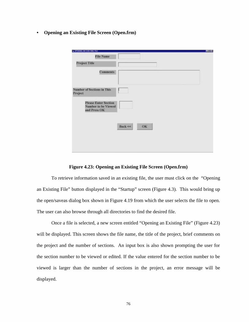
76
• Opening an Existing File Screen (Open.frm)
Figure 4.23: Opening an Existing File Screen (Open.frm)
To retrieve information saved in an existing file, the user must click on the “Opening
an Existing File” button displayed in the “Startup” screen (Figure 4.3). This would bring up
the open/saveas dialog box shown in Figure 4.19 from which the user selects the file to open.
The user can also browse through all directories to find the desired file.
Once a file is selected, a new screen entitled “Opening an Existing File” (Figure 4.23)
will be displayed. This screen shows the file name, the title of the project, brief comments on
the project and the number of sections. An input box is also shown prompting the user for
the section number to be viewed or edited. If the value entered for the section number to be
viewed is larger than the number of sections in the project, an error message will be
displayed.
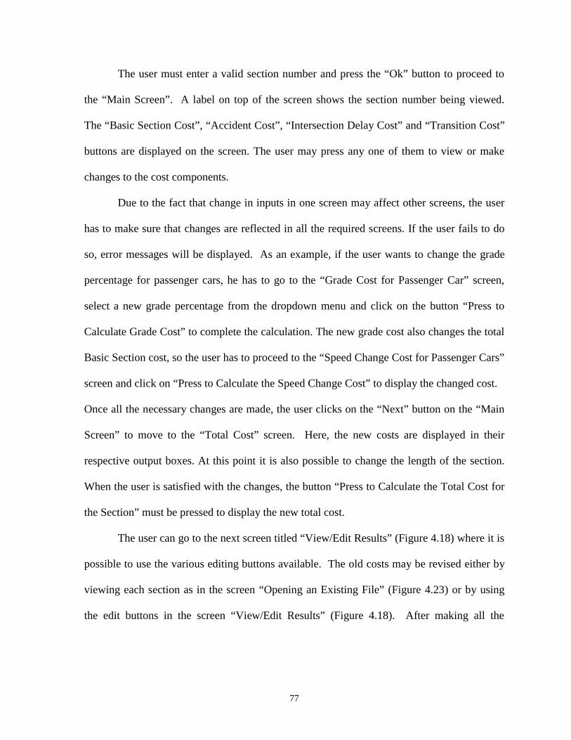
77
The user must enter a valid section number and press the “Ok” button to proceed to
the “Main Screen”. A label on top of the screen shows the section number being viewed.
The “Basic Section Cost”, “Accident Cost”, “Intersection Delay Cost” and “Transition Cost”
buttons are displayed on the screen. The user may press any one of them to view or make
changes to the cost components.
Due to the fact that change in inputs in one screen may affect other screens, the user
has to make sure that changes are reflected in all the required screens. If the user fails to do
so, error messages will be displayed. As an example, if the user wants to change the grade
percentage for passenger cars, he has to go to the “Grade Cost for Passenger Car” screen,
select a new grade percentage from the dropdown menu and click on the button “Press to
Calculate Grade Cost” to complete the calculation. The new grade cost also changes the total
Basic Section cost, so the user has to proceed to the “Speed Change Cost for Passenger Cars”
screen and click on “Press to Calculate the Speed Change Cost” to display the changed cost.
Once all the necessary changes are made, the user clicks on the “Next” button on the “Main
Screen” to move to the “Total Cost” screen. Here, the new costs are displayed in their
respective output boxes. At this point it is also possible to change the length of the section.
When the user is satisfied with the changes, the button “Press to Calculate the Total Cost for
the Section” must be pressed to display the new total cost.
The user can go to the next screen titled “View/Edit Results” (Figure 4.18) where it is
possible to use the various editing buttons available. The old costs may be revised either by
viewing each section as in the screen “Opening an Existing File” (Figure 4.23) or by using
the edit buttons in the screen “View/Edit Results” (Figure 4.18). After making all the
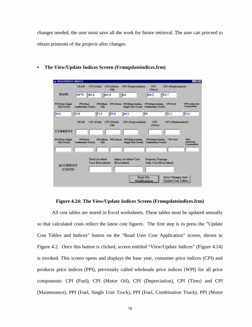
78
changes needed, the user must save all the work for future retrieval. The user can proceed to
obtain printouts of the projects after changes.
• The View/Update Indices Screen (Frmupdateindices.frm)
Figure 4.24: The View/Update Indices Screen (Frmupdateindices.frm)
All cost tables are stored in Excel worksheets. These tables must be updated annually
so that calculated costs reflect the latest cost figures. The first step is to press the ”Update
Cost Tables and Indices” button on the “Road User Cost Application” screen, shown in
Figure 4.2. Once this button is clicked, screen entitled “View/Update Indices” (Figure 4.24)
is invoked. This screen opens and displays the base year, consumer price indices (CPI) and
producer price indices (PPI), previously called wholesale price indices (WPI) for all price
components: CPI (Fuel), CPI (Motor Oil), CPI (Depreciation), CPI (Tires) and CPI
(Maintenance), PPI (Fuel, Single Unit Truck), PPI (Fuel, Combination Truck), PPI (Motor
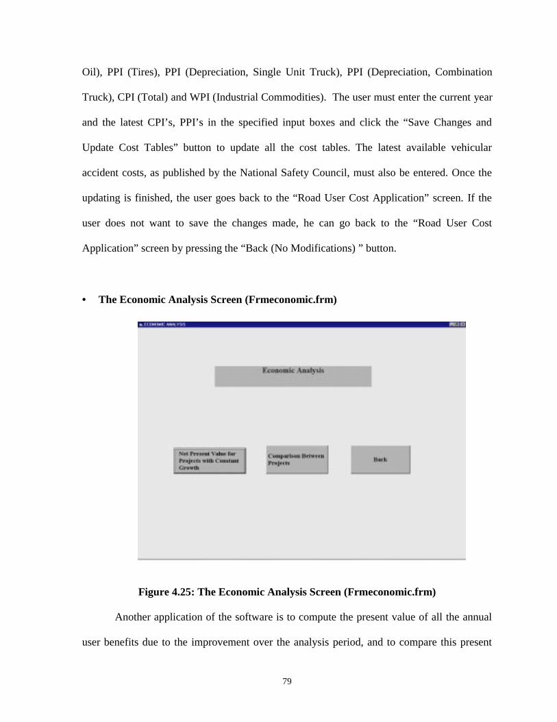
79
Oil), PPI (Tires), PPI (Depreciation, Single Unit Truck), PPI (Depreciation, Combination
Truck), CPI (Total) and WPI (Industrial Commodities). The user must enter the current year
and the latest CPI’s, PPI’s in the specified input boxes and click the “Save Changes and
Update Cost Tables” button to update all the cost tables. The latest available vehicular
accident costs, as published by the National Safety Council, must also be entered. Once the
updating is finished, the user goes back to the “Road User Cost Application” screen. If the
user does not want to save the changes made, he can go back to the “Road User Cost
Application” screen by pressing the “Back (No Modifications) ” button.
• The Economic Analysis Screen (Frmeconomic.frm)
Figure 4.25: The Economic Analysis Screen (Frmeconomic.frm)
Another application of the software is to compute the present value of all the annual
user benefits due to the improvement over the analysis period, and to compare this present
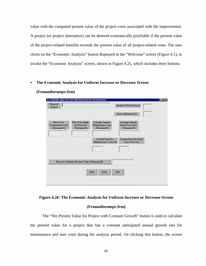
80
value with the computed present value of the project costs associated with the improvement.
A project (or project alternative) can be deemed economically justifiable if the present value
of the project-related benefits exceeds the present value of all project-related costs. The user
clicks on the “Economic Analysis” button displayed in the “Welcome” screen (Figure 4.1), to
invoke the “Economic Analysis” screen, shown in Figure 4.25, which includes three buttons.
• The Economic Analysis for Uniform Increase or Decrease Screen
(Frmuniformnpv.frm)
Figure 4.26: The Economic Analysis for Uniform Increase or Decrease Screen
(Frmuniformnpv.frm)
The “Net Present Value for Project with Constant Growth” button is used to calculate
the present value for a project that has a constant anticipated annual growth rate for
maintenance and user costs during the analysis period. On clicking this button, the screen
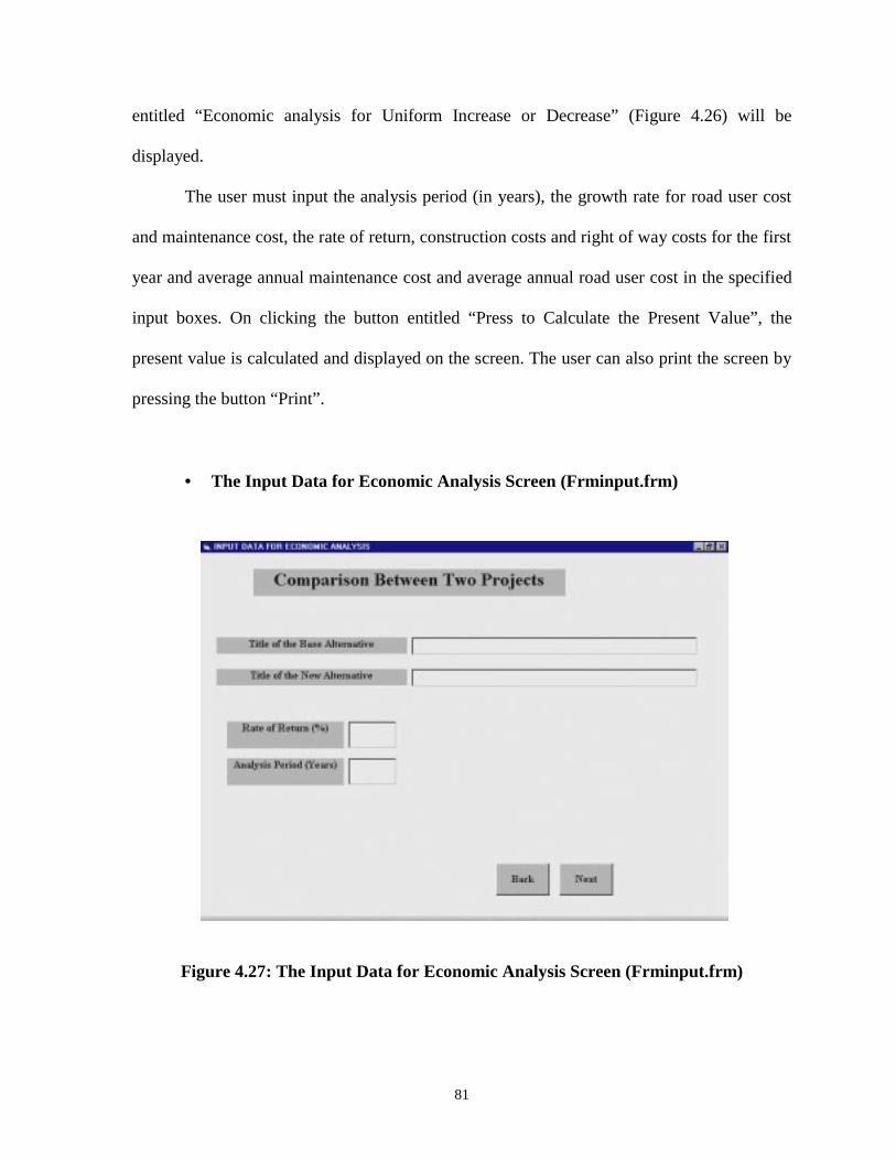
81
entitled “Economic analysis for Uniform Increase or Decrease” (Figure 4.26) will be
displayed.
The user must input the analysis period (in years), the growth rate for road user cost
and maintenance cost, the rate of return, construction costs and right of way costs for the first
year and average annual maintenance cost and average annual road user cost in the specified
input boxes. On clicking the button entitled “Press to Calculate the Present Value”, the
present value is calculated and displayed on the screen. The user can also print the screen by
pressing the button “Print”.
• The Input Data for Economic Analysis Screen (Frminput.frm)
Figure 4.27: The Input Data for Economic Analysis Screen (Frminput.frm)
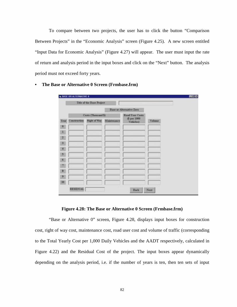
82
To compare between two projects, the user has to click the button “Comparison
Between Projects” in the “Economic Analysis” screen (Figure 4.25). A new screen entitled
“Input Data for Economic Analysis” (Figure 4.27) will appear. The user must input the rate
of return and analysis period in the input boxes and click on the “Next” button. The analysis
period must not exceed forty years.
• The Base or Alternative 0 Screen (Frmbase.frm)
Figure 4.28: The Base or Alternative 0 Screen (Frmbase.frm)
“Base or Alternative 0” screen, Figure 4.28, displays input boxes for construction
cost, right of way cost, maintenance cost, road user cost and volume of traffic (corresponding
to the Total Yearly Cost per 1,000 Daily Vehicles and the AADT respectively, calculated in
Figure 4.22) and the Residual Cost of the project. The input boxes appear dynamically
depending on the analysis period, i.e. if the number of years is ten, then ten sets of input
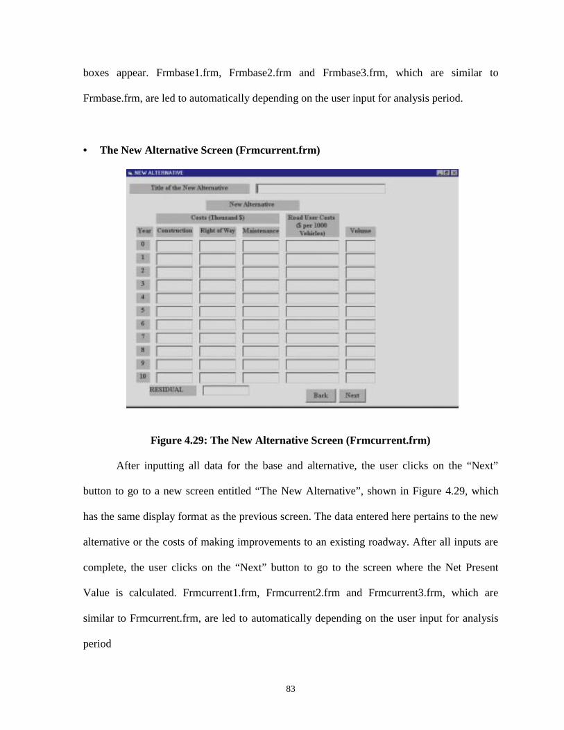
83
boxes appear. Frmbase1.frm, Frmbase2.frm and Frmbase3.frm, which are similar to
Frmbase.frm, are led to automatically depending on the user input for analysis period.
• The New Alternative Screen (Frmcurrent.frm)
Figure 4.29: The New Alternative Screen (Frmcurrent.frm)
After inputting all data for the base and alternative, the user clicks on the “Next”
button to go to a new screen entitled “The New Alternative”, shown in Figure 4.29, which
has the same display format as the previous screen. The data entered here pertains to the new
alternative or the costs of making improvements to an existing roadway. After all inputs are
complete, the user clicks on the “Next” button to go to the screen where the Net Present
Value is calculated. Frmcurrent1.frm, Frmcurrent2.frm and Frmcurrent3.frm, which are
similar to Frmcurrent.frm, are led to automatically depending on the user input for analysis
period
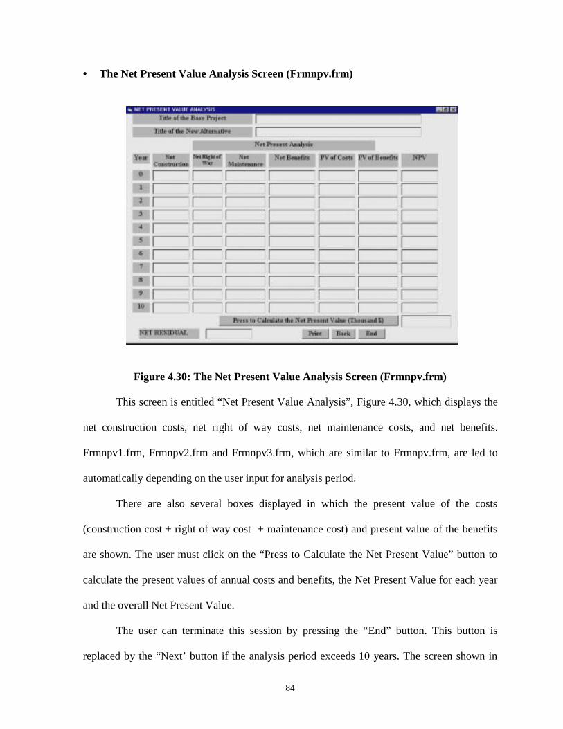
84
• The Net Present Value Analysis Screen (Frmnpv.frm)
Figure 4.30: The Net Present Value Analysis Screen (Frmnpv.frm)
This screen is entitled “Net Present Value Analysis”, Figure 4.30, which displays the
net construction costs, net right of way costs, net maintenance costs, and net benefits.
Frmnpv1.frm, Frmnpv2.frm and Frmnpv3.frm, which are similar to Frmnpv.frm, are led to
automatically depending on the user input for analysis period.
There are also several boxes displayed in which the present value of the costs
(construction cost + right of way cost + maintenance cost) and present value of the benefits
are shown. The user must click on the “Press to Calculate the Net Present Value” button to
calculate the present values of annual costs and benefits, the Net Present Value for each year
and the overall Net Present Value.
The user can terminate this session by pressing the “End” button. This button is
replaced by the “Next’ button if the analysis period exceeds 10 years. The screen shown in
85
Figure 4.30 had an analysis period of 10 years. In short, the last screen would have the “End”
button required to terminate the session.
The code is written in BASIC and each and every form is associated with a code for
carrying out the designated functions. The program code also has a module, which has all the
global functions.
4.3 Database Description
The database having all the cost figures is stored in MS-Excel worksheets. There are
two-database tables. One is named as base.xls and the other is current.xls. Each sheet has
been given a name to identify the type of data stored in it. All the sheets that are present in
the database table base.xls are listed below and the corresponding nomographs and tables
referred from the Manual are described below. The current.xls also has the same sheet
names, the only difference being the cost tables are the updated to the current year.
TRANSITION: The “Transition” sheet holds the data for the transition costs computed by
digitizing the nomograph (Figure 20, pp. 70) of the Manual. The transition cost figures are
used to calculate the transition costs.
TRANADJUST: The “Tranadjust” sheet contains the data for adjusting the transition costs
when trucks, both single unit trucks and 3 S-2 combination trucks are present in the vehicle
mix. The percentages of the two types and the cost factor with which it shall be multiplied
are listed. The table is listed in page 70 of the Manual.
GRADE: The “Grade” sheet contains the database on the grade costs for passenger cars.
This database was constructed by digitizing the nomographs provided in the Manual. It is
function of the grade percent and average running speed. The table is listed as Table B-4,
Page 126 of the Manual.
86
CURVE: The “Curve” sheet contains the costs incurred in negotiating curves on the analysis
section by passenger cars. This cost is a function of the degree of curvature and the average
running speed. The table is listed as Table B-7, Page 129 of the Manual.
PAVEDTOGRAVEL: This sheet contains adjustment factors multiplied to the grade and
curve costs if the road is “Gravel and Stone” type. Figure 19 (pp. 62) of the Manual entitled
“Multiplicative Factors To Convert Motor Vehicle Running Cost On Highway Type
Pavements To Cost On Gravel And Stone Or To Earth Roadway Surfaces” was digitized for
this purpose.
PAVEDTOEARTH: This sheet has the adjustment factors for “Earth” type surface and
these factors are used to adjust the grade and curve costs according to the road type. Figure
19 (pp. 62) of the Manual entitled “Multiplicative Factors To Convert Motor Vehicle
Running Cost On Highway Type Pavements To Cost On Gravel And Stone Or To Earth
Roadway Surfaces” was digitized for this purpose.
ARTERIALSPEEDCHANGECOST: This sheet contains all the cost figures necessary to
calculate the speed change cost for passenger cars in an Arterial type of highway. It includes
the cost figures for a level of service present as well as absent. The nomograph listed on page
53 of the Manual entitled “Basic Section Costs (B) for Passenger Cars on Arterials” was
digitized for this purpose.
TWOLANESPEEDCHANGECOST: This sheet contains data on the speed change cost for
passenger cars in a two-lane or rural highway. It includes the cost figures for a level of
service present as well as absent. The nomograph listed on page 52 of the Manual entitled
“Basic Section Costs (B) for Passenger Cars on Two-Lane Highways” was digitized for this
purpose.
87
MULTILANESPEEDCHANGECOST: This sheet furnishes the data necessary to calculate
the speed change cost for Multi-Lane facility for passenger cars. It includes the cost figures
for a level of service present as well as absent. The nomograph listed on page 51 of the
Manual entitled “Basic Section Costs (B) for Passenger Cars on Multi-Lane Highways” was
digitized for this purpose.
FREEWAYSPEEDCHANGECOST: This sheet contains data on speed change cost for
passenger cars on a Freeway. It includes the cost figures for a level of service present as well
as absent. The nomograph listed on page 50 of the Manual entitled “Basic Section Costs (B)
for Passenger Cars on Freeways” was digitized for this purpose.
TTCARTERIALSF: This sheet has the data for travel time cost for passenger cars on an
Arterial facility with a level of service present. The nomograph listed on page 53 of the
Manual entitled “Basic Section Costs (B) for Passenger Cars on Arterials” was digitized for
this purpose.
TTCARTERIALNOSF: This sheet has the data for travel time cost for passenger cars on an
Arterial facility where level of service is absent. The nomograph listed on page 53 of the
Manual entitled “Basic Section Costs (B) for Passenger Cars on Arterials” was digitized for
this purpose.
TTCTWOLANESF: This sheet contains data on travel time cost for passenger cars on a
two-lane facility with a level of service present. The nomograph listed on page 52 of the
Manual entitled “Basic Section Costs (B) for Passenger Cars on Two-Lane Highways” was
digitized for this purpose.
TTCTWOLANENOSF: This sheet contains data on travel time cost for passenger cars on a
two-lane facility with a level of service absent. The nomograph listed on page 52 of the
88
Manual entitled “Basic Section Costs (B) for Passenger Cars on Two-Lane Highways” was
digitized for this purpose.
TTCMULTISF: This sheet contains data on the travel time cost for passenger cars on a
multi-lane highway with a level of service present. The nomograph listed on page 51 of the
Manual entitled “Basic Section Costs (B) for Passenger Cars on Multi-Lane Highways” was
digitized for this purpose.
TTCMULTINOSF: This sheet contains data on the travel time cost for passenger cars on a
multi-lane highway without a level of service. The nomograph listed on page 51 of the
Manual entitled “Basic Section Costs (B) for Passenger Cars on Multi-Lane Highways” was
digitized for this purpose.
TTCFREEWAYSF: This sheet contains data for travel time cost for passenger cars on a
Freeway having a level of service, F. The nomograph listed on page 50 of the Manual
entitled “Basic Section Costs (B) for Passenger Cars on Freeways” was digitized for this
purpose.
TTCFREEWAYNOSF: This sheet contains data for travel time cost for passenger cars on a
Freeway with a level of service, F absent. The nomograph listed on page 50 of the Manual
entitled “Basic Section Costs (B) for Passenger Cars on Freeways” was digitized for this
purpose.
SPEEDARTERIALNOSF: This sheet contains the average running speed for a passenger
cars on an Arterial facility without level of service. These costs are a function of the vehicle
to capacity ratio and the design speed. The nomograph listed on page 53 of the Manual
entitled “Basic Section Costs (B) for Passenger Cars on Arterials” was digitized for this
purpose.
89
SPEEDTWOLANENOSF: This sheet contains the average running speed for passenger
cars utilizing a two-lane highway without a level of service. These costs are a function of the
vehicle to capacity ratio and the design speed. The nomograph listed on page 52 of the
Manual entitled “Basic Section Costs (B) for Passenger Cars on Two-Lane Highways” was
digitized for this purpose.
SPEEDMULTINOSF: This sheet has cost figures for average running speed of passenger
cars travelling on a Multi-Lane highway without a level of service. These costs are a function
of the vehicle to capacity ratio and the design speed. The nomograph listed on page 51 of the
Manual entitled “Basic Section Costs (B) for Passenger Cars on Multi-Lane Highways” was
digitized for this purpose.
SPEEDFREEWAYNOSF: This sheet has data on average running speed for passenger cars
on a Freeway without a level of service. These costs are a function of the vehicle to capacity
ratio and the design speed. The nomograph listed on page 50 of the Manual entitled “Basic
Section Costs (B) for Passenger Cars on Freeways” was digitized for this purpose.
SPEEDARTERIALSF: This sheet contains the average running speed for passenger cars on
an Arterial facility with a level of service, F. These costs are a function of the vehicle to
capacity ratio and the design speed. The nomograph listed on page 53 of the Manual entitled
“Basic Section Costs (B) for Passenger Cars on Arterials” was digitized for this purpose.
SPEEDTWOLANESF: This sheet contains the average running speed for passenger cars
utilizing a two-lane highway with a level of service, F. These costs are a function of the
vehicle to capacity ratio and the design speed. The nomograph listed on page 52 of the
Manual entitled “Basic Section Costs (B) for Passenger Cars on Two-Lane Highways” was
digitized for this purpose.
90
SPEEDMULTISF: This sheet includes cost figures for average running speed of passenger
cars travelling on a Multi-Lane highway with a level of service, F. These costs are a function
of the vehicle to capacity ratio and the design speed. The nomograph listed on page 51 of the
Manual entitled “Basic Section Costs (B) for Passenger Cars on Multi-Lane Highways” was
digitized for this purpose.
SPEEDFREEWAYSF: This sheet includes data on the cost based on average running speed
for passenger cars on a Freeway with a level of service, F. These costs are a function of the
vehicle to capacity ratio and the design speed. The nomograph listed on page 50 of the
Manual entitled “Basic Section Costs (B) for Passenger Cars on Freeways” was digitized for
this purpose.
AVJSTOPPERVEH: This sheet contains data on the average stops per vehicle (per signal)
on an intersection. It is a function of chi and lambda. The nomograph listed as Figure 21 (pp.
72) of the Manual has been digitized for making this table.
ADDEDSTOPDELAY: This sheet contains figures on the added stopping delay cost per
signal (Time Cost or cost due to Time Value of Money) in an intersection. It is a function of
average length of stop in an intersection and the intersection approach speed. The nomograph
listed as Figure 21 (pp. 72) of the Manual has been digitized for making this table.
DELAYTIMEADJUST: This sheet contains adjustment factors for delay time with respect
to the presence of trucks, both single unit trucks and 3 S-2 combination trucks, when the
added stopping delay cost is computed. This table corresponds to the table listed in page 72
of the Manual.
ADDEDSTOPCOST: This sheet contains data on the added stopping cost per signal
(Running Cost) in an intersection. It is a function of the average stop per vehicles and the
91
approaching speed to a signal on an intersection. The nomograph listed as Figure 21 (pp. 72)
of the Manual has been digitized for making this table.
DELAYCOSTADJUST: This sheet contains adjustment factors for delay time costs with
respect to the presence of trucks, both single unit trucks and 3 S-2 combination trucks, when
the added stopping delay cost is computed. This table corresponds to the table listed in page
72 of the Manual.
IDLINGDELAY: This sheet has the data on the average delay per vehicle and is a function
of chi and the capacity of the road on a signal of an intersection. The nomograph listed as
Figure 22 (pp. 73) has been digitized for making this table.
CYCLETIME: This sheet contains data on the correction to the average delay per vehicle
and is a function of lambda and Cycletime (Signal Cycle Time + Effective Green Time). The
nomograph listed as Figure 22 (pp. 73) has been digitized for making this table.
IDLINGTIME: This sheet contains the time in seconds spent due to idling at intersections.
The nomograph listed as Figure 22 (pp. 73) has been digitized for making this table.
IDLINGTIMECOST: This sheet has the data on cost (Delay Cost due to Time value of
Money) for idling on a signal on an intersection and is a function of time (Idling time). The
nomograph listed as Figure 22 (pp. 73) has been digitized for making this table.
IDLINGTIMEADJUST: This sheet contains adjustment factors for delay time costs with
respect to the presence of trucks, both single unit trucks and 3 S-2 combination trucks, when
the delay cost is computed. This table corresponds to the table listed in page 73 of the
Manual.
92
IDLINGCOST: This sheet has the data on cost (Idling Cost) for idling on a signal on an
intersection and is a function of time (Idling time at an Intersection). The nomograph listed as
Figure 22 (pp. 73) has been digitized for making this table.
IDLINGCOSTADJUST: This sheet contains adjustment factors for delay time costs with
respect to the presence of trucks, both single unit trucks and 3 S-2 combination trucks, when
the idling cost is computed. This table corresponds to the table listed in page 73 of the
Manual.
ACCIDENTCOSTS: This sheet contains the latest vehicular accident costs for the Fatal
Accident, Injury Accident and Property Damage Only type of accident.
CPIINDICES: This sheet has the consumer price indices and producer price indices on
which the database is based upon. If the latest consumer price indices are available, the user
must update the database based on the given provisions. The latest cost factors replaces the
old factors once the update is done in current.xls.
SUTGRADE: This sheet contains the database on the grade costs for single unit trucks. This
database was constructed by digitizing the nomographs provided in the Manual. It is function
of the grade percent and average running speed. The table is listed as Table B-5, Page 127 of
the Manual.
SUTCURVE: This sheet contain the costs due to curves incurred in negotiating curves on
the analysis section by single unit trucks. This cost is a function of the degree of curvature
and the average running speed. The table is listed as Table B-8, Page 130 of the Manual.
SUTARTERIALSPEEDCHANGECOST: This sheet contains all the cost figures
necessary in calculating the speed change cost for single unit trucks in Arterial type of
highway. It includes the cost figures for a level of service present as well as absent. The
93
nomograph listed on page 57 of the Manual entitled “Basic Section Costs (B) for Single Unit
Trucks on Arterials” was digitized for this purpose.
SUTTWOLANESPEEDCHANGECOST: This sheet contains data on the speed change
cost for single unit trucks in a two-lane or rural highway. It includes the cost figures for a
level of service present as well as absent. The nomograph listed on page 56 of the Manual
entitled “Basic Section Costs (B) for Single Unit Trucks on Two-Lane Highways” was
digitized for this purpose.
SUTMULTILANESPEEDCHANGECOST: This sheet furnishes the data necessary to
calculate the speed change cost for Multi-Lane facility for single unit trucks. It includes the
cost figures for a level of service present as well as absent. The nomograph listed on page 55
of the Manual entitled “Basic Section Costs (B) for Single Unit Trucks on Multi-Lane
Highways” was digitized for this purpose.
SUTFREEWAYSPEEDCHANGECOST: This sheet contains data on speed change cost
for single unit trucks on a Freeway. It includes the cost figures for a level of service present
as well as absent. The nomograph listed on page 54 of the Manual entitled “Basic Section
Costs (B) for Single Unit Trucks on Freeways” was digitized for this purpose.
SUTTTCARTERIALSF: This sheet has the data for travel time cost for single unit trucks
on an Arterial facility with a level of service. The nomograph listed on page 57 of the Manual
entitled “Basic Section Costs (B) for Single Unit Trucks on Arterials” was digitized for this
purpose.
SUTTTCARTERIALNOSF: This sheet has the data for travel time cost for single unit
trucks on an Arterial facility without a level of service. The nomograph listed on page 57 of
94
the Manual entitled “Basic Section Costs (B) for Single Unit Trucks on Arterials” was
digitized for this purpose.
SUTTTCTWOLANESF: This sheet contains data on travel time cost for single unit trucks
on a two-lane facility with a level of service, F. The nomograph listed on page 56 of the
Manual entitled “Basic Section Costs (B) for Single Unit Trucks on Two-Lane Highways”
was digitized for this purpose.
SUTTTCTWOLANENOSF: This sheet contains data on travel time cost for single unit
trucks on a two-lane facility without a level of service. The nomograph listed on page 56 of
the Manual entitled “Basic Section Costs (B) for Single Unit Trucks on Two-Lane
Highways” was digitized for this purpose.
SUTTTCMULTISF: This sheet contains data on the travel time cost for single unit trucks
on a Multi-Lane highway with a level of service, F. The nomograph listed on page 55 of the
Manual entitled “Basic Section Costs (B) for Single Unit Trucks on Multi-Lane Highways”
was digitized for this purpose.
SUTTTCMULTINOSF: This sheet contains data on the travel time cost for single unit
trucks on a Multi-Lane highway without a level of service. The nomograph listed on page 55
of the Manual entitled “Basic Section Costs (B) for Single Unit Trucks on Multi-Lane
Highways” was digitized for this purpose.
SUTTTCFREEWAYSF: This sheet contains data for travel time cost for single unit trucks
on a Freeway having a level of service, F. The nomograph listed on page 54 of the Manual
entitled “Basic Section Costs (B) for Single Unit Trucks on Freeways” was digitized for this
purpose.
95
SUTTTCFREEWAYNOSF: This sheet contains data for travel time cost for single unit
trucks on a Freeway having a level of service. The nomograph listed on page 54 of the
Manual entitled “Basic Section Costs (B) for Single Unit Trucks on Freeways” was digitized
for this purpose.
SUTSPEEDARTERIALNOSF: This sheet contains the average running speed for single
unit trucks on an Arterial facility without level of service. These costs are a function of the
vehicle to capacity ratio and the design speed. The nomograph listed on page 57 of the
Manual entitled “Basic Section Costs (B) for Single Unit Trucks on Arterials” was digitized
for this purpose.
SUTSPEEDTWOLANENOSF: This sheet contains the average running speed for a single
unit trucks utilizing the Two-Lane highway without a level of service. These costs are a
function of the vehicle to capacity ratio and the design speed. The nomograph listed on page
56 of the Manual entitled “Basic Section Costs (B) for Single Unit Trucks on Two-Lane
Highways” was digitized for this purpose.
SUTSPEEDMULTINOSF: This sheet has cost figures for average running speed of single
unit trucks travelling on a Multi-Lane highway without a level of service. These costs are a
function of the vehicle to capacity ratio and the design speed. The nomograph listed on page
55 of the Manual entitled “Basic Section Costs (B) for Single Unit Trucks on Multi-Lane
Highways” was digitized for this purpose.
SUTSPEEDFREEWAYNOSF: This sheet has data on average running speed single unit
trucks on a Freeway without a level of service. These costs are a function of the vehicle to
capacity ratio and the design speed. The nomograph listed on page 54 of the Manual entitled
“Basic Section Costs (B) for Single Unit Trucks on Freeways” was digitized for this purpose.
96
SUTSPEEDARTERIALSF: This sheet contains the average running speed for single unit
trucks on an Arterial facility with a level of service, F. These costs are a function of the
vehicle to capacity ratio and the design speed. The nomograph listed on page 57 of the
Manual entitled “Basic Section Costs (B) for Single Unit Trucks on Arterials” was digitized
for this purpose.
SUTSPEEDTWOLANESF: This sheet contains the average running speed for a single unit
trucks utilizing the Two-Lane highway with a level of service, F. These costs are a function
of the vehicle to capacity ratio and the design speed. The nomograph listed on page 56 of the
Manual entitled “Basic Section Costs (B) for Single Unit Trucks on Two-Lane Highways”
was digitized for this purpose.
SUTSPEEDMULTISF: This sheet has cost figures for average running speed of single unit
trucks travelling on a Multi-Lane highway with a level of service, F. These costs are a
function of the vehicle to capacity ratio and the design speed. The nomograph listed on page
55 of the Manual entitled “Basic Section Costs (B) for Single Unit Trucks on Multi-Lane
Highways” was digitized for this purpose.
SUTSPEEDFREEWAYSF: This sheet has data on average running speed single unit trucks
on a Freeway with a level of service, F. These costs are a function of the vehicle to capacity
ratio and the design speed. The nomograph listed on page 54 of the Manual entitled “Basic
Section Costs (B) for Single Unit Trucks on Freeways” was digitized for this purpose.
CTGRADE: This sheet contains the database on the grade costs for 3 S-2 combination
trucks. This database was constructed by digitizing the nomographs provided in the Manual.
It is function of the grade percent and average running speed. The table is listed as Table B-6,
Page 128 of the Manual.
97
CTCURVE: This sheet contains the costs due to curves incurred in negotiating curves on the
analysis section by 3 S-2 combination trucks. This cost is a function of the degree of
curvature and the average running speed. The table is listed as Table B-9, Page 131 of the
Manual.
CTARTERIALSPEEDCHANGECOST: This sheet contains all the cost figures necessary
in calculating the speed change cost for a 3 S-2 combination trucks in Arterial type of
highway. It includes the cost figures for a level of service present as well as absent. The
nomograph listed on page 61 of the Manual entitled “Basic Section Costs (B) for 3-S2
Combination Trucks on Arterials” was digitized for this purpose.
CTTWOLANESPEEDCHANGECOST: This sheet contains data on the speed change cost
for a 3 S-2 combination trucks in a two-lane or rural highway. It includes the cost figures for
a level of service present as well as absent. The nomograph listed on page 60 of the Manual
entitled “Basic Section Costs (B) for 3-S2 Combination Trucks on Two-Lane Highways” was
digitized for this purpose.
CTMULTLANESPEEDCHANGECOST: This sheet furnishes the data necessary to
calculate the speed change cost for Multi-Lane facility for 3 S-2 combination trucks. It
includes the cost figures for a level of service present as well as absent. The nomograph
listed on page 59 of the Manual entitled “Basic Section Costs (B) for 3-S2 Combination
Trucks on Multi-Lane Highways” was digitized for this purpose.
CTFREEWAYSPEEDCHANGECOST: This sheet contains data on speed change cost for
3 S-2 combination trucks on a Freeway. It includes the cost figures for a level of service
present as well as absent. The nomograph listed on page 58 of the Manual entitled “Basic
Section Costs (B) for 3-S2 Combination Trucks on Freeways” was digitized for this purpose.
98
CTTTCARTERIALSF: This sheet has the data for travel time cost for 3 S-2 combination
trucks on an Arterial facility with a level of service. The nomograph listed on page 61 of the
Manual entitled “Basic Section Costs (B) for 3-S2 Combination Trucks on Arterials” was
digitized for this purpose.
CTTTCARTERIALNOSF: This sheet has the data for travel time cost for 3 S-2
combination trucks on an Arterial facility without a level of service. The nomograph listed on
page 61 of the Manual entitled “Basic Section Costs (B) for 3-S2 Combination Trucks on
Arterials” was digitized for this purpose.
CTTTCTWOLANESF: This sheet contains data on travel time cost for 3 S-2 combination
trucks on a two-lane facility with a level of service, F. The nomograph listed on page 60 of
the Manual entitled “Basic Section Costs (B) for 3-S2 Combination Trucks on Two-Lane
Highways” was digitized for this purpose.
CTTTCTWOLANENOSF: This sheet contains data on travel time cost for 3 S-2
combination trucks on a two-lane facility without a level of service. The nomograph listed on
page 60 of the Manual entitled “Basic Section Costs (B) for 3-S2 Combination Trucks on
Two-Lane Highways” was digitized for this purpose.
CTTTCMULTISF: This sheet contains data on the travel time cost for 3 S-2 combination
trucks on a multi-lane highway with a level of service, F. The nomograph listed on page 59
of the Manual entitled “Basic Section Costs (B) for 3-S2 Combination Trucks on Multi-Lane
Highways” was digitized for this purpose.
CTTTCMULTINOSF: This sheet contains data on the travel time cost for 3 S-2
combination trucks on a multi-lane highway without a level of service. The nomograph listed
99
on page 59 of the Manual entitled “Basic Section Costs (B) for 3-S2 Combination Trucks on
Multi-Lane Highways” was digitized for this purpose.
CTTTCFREEWAYSF: This sheet contains data for travel time cost for 3 S-2 combination
trucks on a freeway having a level of service, F. The nomograph listed on page 58 of the
Manual entitled “Basic Section Costs (B) for 3-S2 Combination Trucks on Freeways” was
digitized for this purpose.
CTTTCFREEWAYNOSF: This sheet contains data for travel time cost for 3 S-2
combination trucks on a Freeway having a level of service. The nomograph listed on page 58
of the Manual entitled “Basic Section Costs (B) for 3-S2 Combination Trucks on Freeways”
was digitized for this purpose.
CTSPEEDARTERIALNOSF: This sheet contains the average running speed for a 3 S-2
combination trucks on an Arterial facility without level of service. These costs are a function
of the vehicle to capacity ratio and the design speed. The nomograph listed on page 61 of the
Manual entitled “Basic Section Costs (B) for 3-S2 Combination Trucks on Arterials” was
digitized for this purpose.
CTSPEEDTWOLANENOSF: This sheet contains the average running speed for 3 S-2
combination trucks utilizing the Two-Lane highway without a level of service. These costs
are a function of the vehicle to capacity ratio and the design speed. The nomograph listed on
page 60 of the Manual entitled “Basic Section Costs (B) for 3-S2 Combination Trucks on
Two-Lane Highways” was digitized for this purpose.
CTSPEEDMULTINOSF: This sheet has cost figures for average running speed of 3 S-2
combination trucks travelling on a Multi-Lane highway without a level of service. These
costs are a function of the vehicle to capacity ratio and the design speed. The nomograph
100
listed on page 59 of the Manual entitled “Basic Section Costs (B) for 3-S2 Combination
Trucks on Multi-Lane Highways” was digitized for this purpose.
CTSPEEDFREEWAYNOSF: This sheet has data on average running speed 3 S-2
combination trucks on a Freeway without a level of service. These costs are a function of the
vehicle to capacity ratio and the design speed. The nomograph listed on page 58 of the
Manual entitled “Basic Section Costs (B) for 3-S2 Combination Trucks on Freeways” was
digitized for this purpose.
CTSPEEDARTERIALSF: This sheet contains the average running speed for 3 S-2
combination trucks on an Arterial facility with a level of service, F. These costs are a
function of the vehicle to capacity ratio and the design speed. The nomograph listed on page
61 of the Manual entitled “Basic Section Costs (B) for 3-S2 Combination Trucks on
Arterials” was digitized for this purpose.
CTSPEEDTWOLANESF: This sheet contains the average running speed for a 3 S-2
combination trucks utilizing the Two-Lane highway with a level of service, F. These costs
are a function of the vehicle to capacity ratio and the design speed. The nomograph listed on
page 60 of the Manual entitled “Basic Section Costs (B) for 3-S2 Combination Trucks on
Two-Lane Highways” was digitized for this purpose.
CTSPEEDMULTISF: This sheet has cost figures for average running speed of 3 S-2
combination trucks travelling on a Multi-Lane highway with a level of service, F. These costs
are a function of the vehicle to capacity ratio and the design speed. The nomograph listed on
page 59 of the Manual entitled “Basic Section Costs (B) for 3-S2 Combination Trucks on
Multi-Lane Highways” was digitized for this purpose.
101
CTSPEEDFREEWAYSF: This sheet has data on average running speed for 3 S-2
combination trucks on a Freeway with a level of service, F. These costs are a function of the
vehicle to capacity ratio and the design speed. The nomograph listed on page 58 of the
Manual entitled “Basic Section Costs (B) for 3-S2 Combination Trucks on Freeways” was
digitized for this purpose.
4.4 Internal Working and the File Structure
This section describes the internal working of the software. The Visual Basic 5
project is stored in a file named HighwayCosts.vbp. This file is converted to an executable
file titled “HighwayCosts.exe”. This is an executable file meaning that the source code is not
available for editing. The executable file includes all the system files (.sys files), dynamic
link library files (.dll files) and ActiveX control files (.ocx files). All of the files needed to
install the software are available in the Setup.exe. Once the Setup.exe file is run, the setup
wizard is activated. It tells in a systematic manner how to install the software and dependent
files including the database. The database is stored in two files. The 1975 cost tables are
stored in a file named base.xls and the latest cost tables after updating from 1975 cost tables
are stored in current.xls. The base.xls and the current.xls files are stored in a directory labeled
“Database”. The setup files are located in the directory called “Setup”. These files are already
installed on the West Virginia Division of Highway server.
The software works when the HighwayCosts.vbp file (The Visual Basic 5 Project
file) which has all the forms and module binds to the database using the Data Control
Objects. These establish a link between the user and the database. Different tables are
accessed according to the input characteristics. Sets of interpolation are carried out to
102
compute the costs when the inputs are intermediate between two points in the nomographs.
Extrapolation is strictly avoided because the characteristic of the graph is unknown beyond
the end points. The software source code and its various components are included in the
appendices.
Updating technique is based on the formulas described in Chapter 3. Updating is
always done with the 1975 cost tables as the base to minimize round off errors. This is the
reason base.xls file (the file having the 1975 cost tables) is present along with the current
price table (current.xls). When the user chooses to update the cost tables, a connection is
established with the base.xls file. Costs are updated according to the formulas described in
Chapter 3. As soon as the updating is done, the base.xls is saved as current.xls dynamically
by the code written. This ensures that the base.xls file stays unchanged and a new current.xls
is created and ready for referral.
4.5 Valid Ranges for Inputs and Parameters
User inputs have to be consistent and valid for the proper functioning of the software.
Also, calculations can be completed only if all the required inputs are entered. Several
displays and error messages are designed to alert the user in case of missing or inconstitent
inputs. In the following, a number of possible inconsistencies are discussed.
The set of valid inputs to the software and their ranges are described in this section. It
is important that the inputs be within the ranges specified in order to produce correct results.
If the inputs are out of range, a warning message will be displayed as “Inputs Out of Range”.
At this point the user is asked to reenter a valid input before the user can proceed.
The maximum number of sections that can be analyzed for a project is limited to 50.
This limit has been determined in consultation with the WVDOH officials. Entering a project
103
title is mandatory. The vehicle mix must consist of passenger cars. Percentages of Single
Unit Trucks and 3 S-2 Combination Trucks must be entered even if they are equal to zero.
The Basic Section Cost starts with computing the average running speed. The user
must select a unique facility and a corresponding service level (F) of yes (Service Level F is
present) or no (Service Level F is not present). The volume to capacity ratio ranges from 0 to
1 in increments of 0.10. The design speed for Freeway facility is 70 mph, 60 mph and 50
mph. This is the same for a Multi-Lane highway facility. The design speed for two-lane
highway ranges from 40 mph to 70 mph in increments of 10 mph. An Arterial facility has a
range of 25 mph to 45 mph in increments of 10 mph. These values are the same for single
unit trucks and 3 S-2 combination trucks.
To compute the travel time cost, the user must enter the hourly value of time in
dollars. The grade costs are a function of the average running speed and grade percentages.
The grade percentage ranges from –8 to 8 in increments of one unit. That means that a grade
percent of 0.5 would be a wrong input.
The curve costs is a function of the average running speed and degree of curvature.
The curve ranges from 1 to 30. This range of values applies also to single unit trucks and 3-
S-2 combination trucks.
Transition costs depend on the initial speed and speed reduced and returned to. Valid
values for the initial speed range from 80 mph to 5 mph in increments of 5 mph. The reduced
and returned to speed ranges from 75 mph to 0 mph (complete stop) in increments of 5 mph.
Intersection delay cost depends on the volume of the traffic on the road at the
intersection, capacity of the road, signal cycle time, effective green time and the intersection
approach speed (the range is from 5 mph to 55 mph). Intermediate values such as lambda,
104
capacity of approach and chi are computed depending on the above inputs. These inputs must
be such that the intermediate values computed fall in specific ranges. The value of computed
lambda must be between 0.2 and 0.8. The value of capacity of approach is between 200 and
4,400. The value of chi is between 0.1 and 0.8.
The above mentioned ranges conform to the nomographs given in the Manual and
must be strictly followed.
In most cases, the user is required to enter a value for a variable or choose from a
drop-down menu. If the value entered is not included in the drop-down menu, the software
will not respond. For example, valid choices for the design speed for a Freeway are 70 miles
per hour, 60 miles per hour and 50 miles per hour. Any speed other than the above-
mentioned values, such as 65 miles per hour, will result in the software not responding to the
input. Another example is the user input for vehicle to capacity ratio. It has a range from 0 to
1 in steps of 0.1. An input of 0.25 would be considered inconstitent. The software also
assumes that percentage of cars is greater than zero for every section of a project. An input
of zero percent for cars will cause an error message to be displayed.
4.6 Example
The following example illustrates the use of the software. The software essentially
does three tasks, namely calculating the user costs for a highway project, update the costs so
that the most recent cost tables are used, and perform an economic analysis to determine
project feasibility and comparison of alternatives.
The user enters the number of section in the screen shown in Figure 4.4. In this
example, the title of the project is Morgantown-Grafton and the number of section is 1.
Inputs for Basic Section cost shown in Table 4.2 are common for all type of vehicles
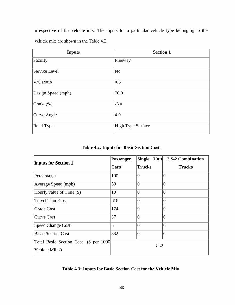
105
irrespective of the vehicle mix. The inputs for a particular vehicle type belonging to the
vehicle mix are shown in the Table 4.3.
Inputs Section 1
Facility Freeway
Service Level No
V/C Ratio 0.6
Design Speed (mph) 70.0
Grade (%) -3.0
Curve Angle 4.0
Road Type High Type Surface
Table 4.2: Inputs for Basic Section Cost.
Inputs for Section 1Passenger
Cars
Single Unit
Trucks
3 S-2 Combination
Trucks
Percentages 100 0 0
Average Speed (mph) 50 0 0
Hourly value of Time ($) 10 0 0
Travel Time Cost 616 0 0
Grade Cost 174 0 0
Curve Cost 37 0 0
Speed Change Cost 5 0 0
Basic Section Cost 832 0 0
Total Basic Section Cost ($ per 1000
Vehicle Miles)832
Table 4.3: Inputs for Basic Section Cost for the Vehicle Mix.
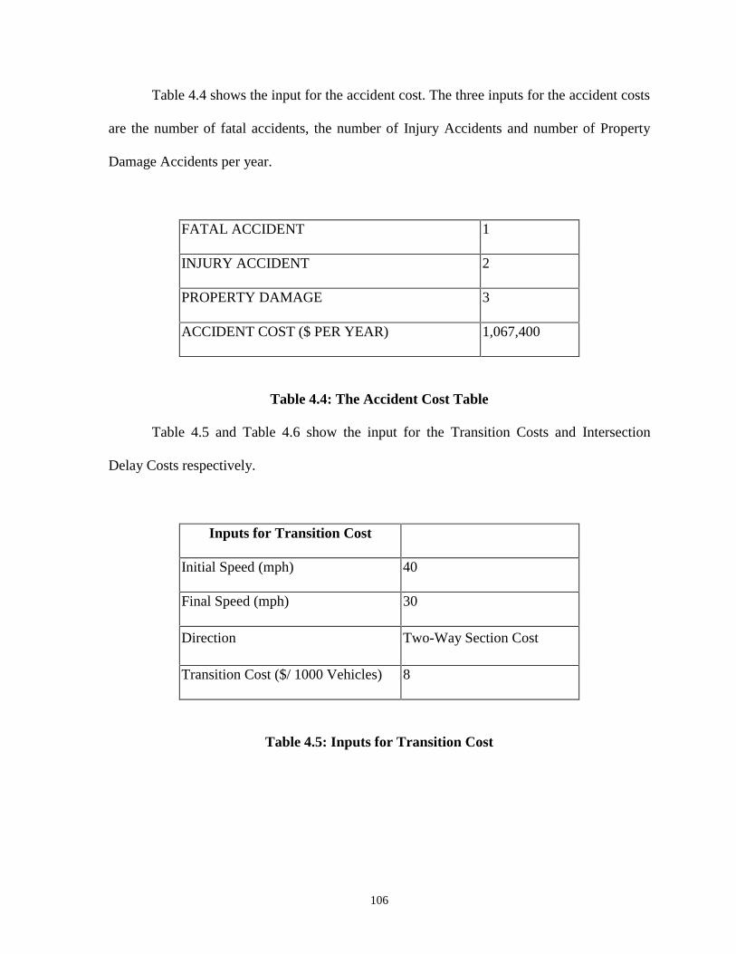
106
Table 4.4 shows the input for the accident cost. The three inputs for the accident costs
are the number of fatal accidents, the number of Injury Accidents and number of Property
Damage Accidents per year.
FATAL ACCIDENT 1
INJURY ACCIDENT 2
PROPERTY DAMAGE 3
ACCIDENT COST ($ PER YEAR) 1,067,400
Table 4.4: The Accident Cost Table
Table 4.5 and Table 4.6 show the input for the Transition Costs and Intersection
Delay Costs respectively.
Inputs for Transition Cost
Initial Speed (mph) 40
Final Speed (mph) 30
Direction Two-Way Section Cost
Transition Cost ($/ 1000 Vehicles) 8
Table 4.5: Inputs for Transition Cost
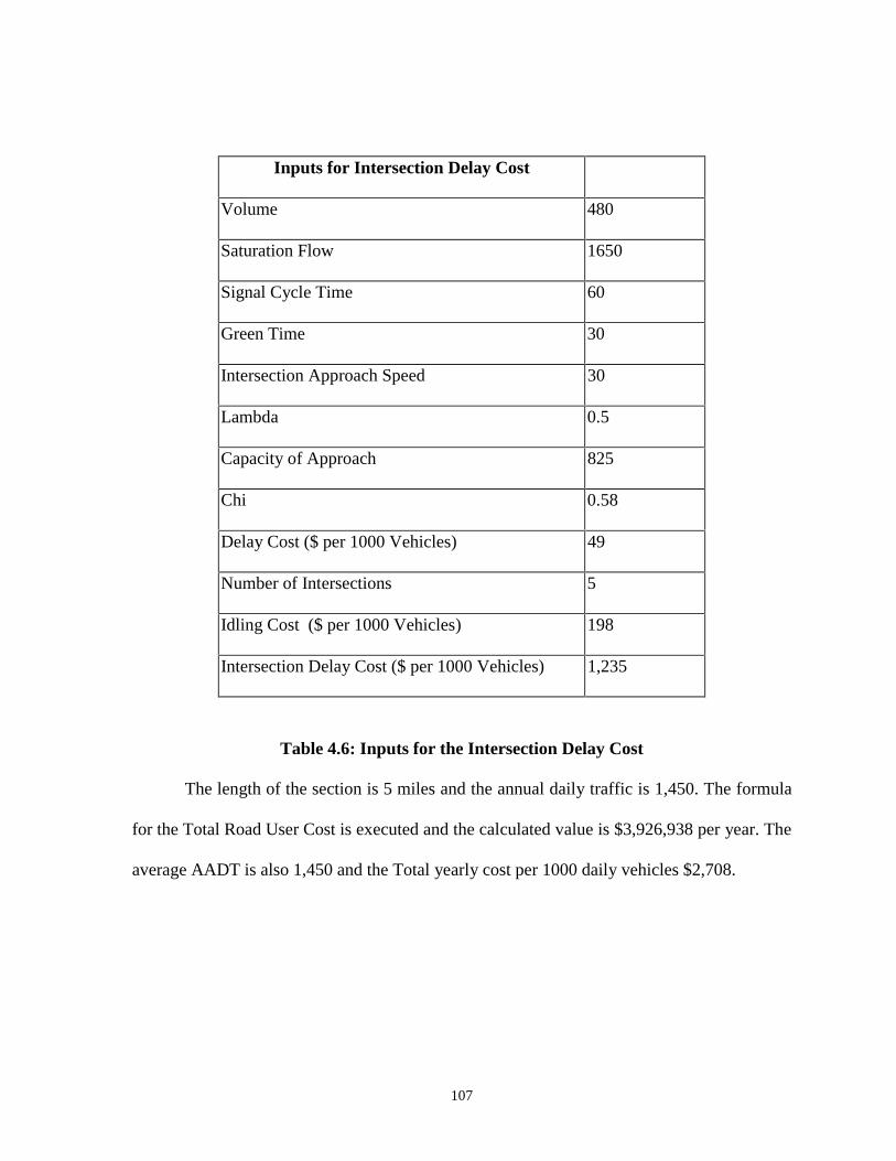
107
Inputs for Intersection Delay Cost
Volume 480
Saturation Flow 1650
Signal Cycle Time 60
Green Time 30
Intersection Approach Speed 30
Lambda 0.5
Capacity of Approach 825
Chi 0.58
Delay Cost ($ per 1000 Vehicles) 49
Number of Intersections 5
Idling Cost ($ per 1000 Vehicles) 198
Intersection Delay Cost ($ per 1000 Vehicles) 1,235
Table 4.6: Inputs for the Intersection Delay Cost
The length of the section is 5 miles and the annual daily traffic is 1,450. The formula
for the Total Road User Cost is executed and the calculated value is $3,926,938 per year. The
average AADT is also 1,450 and the Total yearly cost per 1000 daily vehicles $2,708.
108
Chapter 5: Conclusions and Recommendations for Future Research
5.1 Conclusions
“A Manual on User Benefit Analysis of Highway and Bus-Transit Improvements ”
published in 1977 by AASHTO provides guidelines for road user cost. Unfortunately, the use
of the Manual is cumbersome and error-prone. In order to address this problem, an
application software was developed based on the 1977 Manual. The 1977 Manual is a
product of research sponsored by NCHRP. The project entitled “Highway User Economic
Analysis” was performed under NCHRP Project 2-12 and formed the basis for the cost tables
and nomographs in the Manual.
The application software reported here was been developed for the WVDOH to
facilitate the computation of road-user cost, which forms one of the most important
components of the highway transportation costs. Federal regulations require all state
departments of transportation to conduct an economic analysis for all projects costing over
twenty five million dollars.
This software provides highway planners with easy to use capabilities to perform
benefit-cost analysis for individual projects as well as compare various alternatives based on
several engineering economy criteria. This software can be used to compute the road user
cost for a project with up to fifty sections with varying characteristics. The road user cost are
calculated as annualized costs. Provisions are made for updating the cost tables as the latest
consumer price indices and producer price indices become available. Net Present Value
analysis has been used as an engineering economy tool to conduct the economic analysis. All
components of costs that are incurred over the life cycle of a project are included in the
109
economic analysis. These include construction costs, maintenance costs, right of way costs,
residual costs and road user cost.
Visual Basic 5 has proved to be an effective front-end tool interacting with the
database tables stored in Microsoft Excel. The software can be used to perform analysis on
new projects as well as those which have been analyzed previously and saved in a file. The
user can also add, delete, or modify a section as and when required.
5.2 Recommendations for Future Research
A lot of research is going on in the field of Engineering Economy. New concepts are
born that can be used to further enhance the basis for economic justification of a project. Net
Present Value method can be used to decide whether a project is economically feasible or
not; but it alone cannot justify economic decisions. Enhanced version of the Net Present
Value techniques, which may include probabilistic approaches and risk factor analysis, can
be incorporated in future research.
New software application can be developed to integrate the current application with
other highway evaluation applications. Various manuals such as the Highway Capacity
Manual can be consulted dynamically. The current application can be further developed into
a full-fledged decision support system. As an extension of this project, it is also
recommended to make this application web-based so that other state DOT’s can use it.
110
References
1. American Association of State Highway Officials. (1952). Road User Cost Benefit
Analysis Improvements. Washington, DC.
2. Anderson, D. G., Curry, D. A., and Pozdena, R. J. (1977). User Benefit Analysis for
Highway and Bus Transit Improvements. Final Report NCHRP Project 2-12, Stanford
Research Institute, Meleno Park, CA. (Published as A Manual on User Benefit Analysis
of Highway and Bus-Transit Improvements, 1977 by the American Association of State
Highway and Transportation Officials).
3. Bureau of Labor Statistics. [On-Line]. Available: http://www.bls.gov
4. Claffey, P. J. (1971). Running Costs of Motor Vehicles as Affected by Road Design and
Traffic, National Cooperative Highway Research Program (NCHRP) Report No. 111.
5. Curry, D. A., and Anderson, D. G. (1972). Procedures for Estimating Highway User
Costs, Air Pollution, and Noise Effects, National Cooperative Highway Research
Program (NCHRP) Report No. 133. pp.127.
6. DeCorla-Souza, P., Cohen, H., Haling, D., and Hunt, J. (1997). Using Steam for Benefit-
Cost Analysis of Transportation Alternatives, Prepared for Consideration for presentation
at the 1998 Annual Meeting of the Transportation Research Board, Paper No. 980083.
pp.1-7.
7. Dell’Isola, A. J. and Kirk, S. J. (1981). Life Cycle Costing for Design Professionals. New
York. McGraw-Hill.
8. Douglas H. (1997). Visual Basic 5 Bible. CA. IDG Books Worldwide, Inc.
9. Federal Highway Administration (1994). Highway Economy Requirements System
(HERS)-Overview. Volume 2.
111
10. Federal Highway Administration (1995). Highway Economy Requirements System
(HERS)-User’s Guide. Volume 3.
11. Federal Highway Administration (1996). Highway Economy Requirements System
(HERS)-Technical Report. Volume 4.
12. Federal Highway Administration Policy Memorandum (1996). National Highway System
Designation Act. Life-Cycle Cost Analysis Requirements. [On-Line]. Available:
http://www.fhwa.dot.gov/legsreg/directives/policy/lcca.htm
13. Frye, F. F. (1973). Alternative Multimodal Passenger transportation Systems-A
Comparative Analysis. National Cooperative Highway Research Program (NCHRP).
Report 146. pp.68.
14. Hickling Lewis Brod, Inc. StratBENCOST. [On-Line]. Available: http://www.hlb-
econ.com/web1/prod02.htm
15. Lindow, E. S. (1978). Systems Approach to Life-Cycle Design of Pavements, Vol 1, Life
2 Users Manual, Report No. CERL-TR-M-253, Construction Engineering Research
Laboratory, Dept of Army.
16. National Cooperative Highway Research Program (1993). MicroBENCOST User’s
Manual. Project 7-12, Texas Transportation Institute, The Texas A&M University
System. College Station, Texas.
17. National Cooperative Highway Research Program. Microcomputer Evaluation of
Highway User Benefits. Project 7-12. [On-Line]. Available:
http://www2.nas.edu/trbcrp/25a2.html

112
18. National Cooperative Highway Research Program. Research Strategies for Improving
Highway User Cost-Estimating Methodologies. Project 2-18. [On-Line]. Available:
http://www2.nas.edu/trbcrp/689a.html
19. National Cooperative Highway Research Program. Development of an Innovative
Highway User-Cost Estimation Procedure. Project 2-18/3. [On-Line]. Available:
http://www2.nas.edu/trbcrp/68fa.html
20. National Cooperative Highway Research Program (1998). Summary of Progress,
Transportation Research Board, National Research Council. Washington, DC.
21. National Safety Council (1997). Estimating the Cost of Unintentional Injuries. [On-Line].
Available: http://www.nsc.org/lrs/statinfo/estcost7.htm
22. Oglesby, C. H. and Hicks, R. G. (1982). Highway Engineering. (4th Edition). New York.
Wiley.
23. Peterson, D. E. (1985). Life-Cycle Cost Analysis of Pavements, National Cooperative
Highway Research Program Synthesis of Highway Practice, Highway Research Board,
National Research Council.
24. Stanford Research Institute (1961). Economics of Asphalt and Concrete for Highway
Construction. Report No. SRI Project IE-3153, American Petroleum Institute, New York.
25. Thomas, E. N. and Schofer, J. L. (1970). Strategies for the Evaluation of the Alternative
Transportation Plans. National Cooperative Highway Research Council (NCHRP).
Report 96. pp.111.
26. Winfrey, R., and Zellner, C. (1971). Summary and Evaluation of Economic
Consequences of Highway Improvements, National Cooperative Highway Research
Program (NCHRP) Report No. 122. pp.324.

113
27. Winfrey, R. (1968). Economic Analysis for Highways. Scranton, PA. International
Textbook.
28. Wright, H. P (1996). Highway Engineering. (6th Edition). New York. John Wiley &
Sons, Inc.
114
Appendix A: Software Manual
West Virginia Department of Transportation
Division of Highways
Highway Cost-Benefit Analysis System
Software User’s Manual
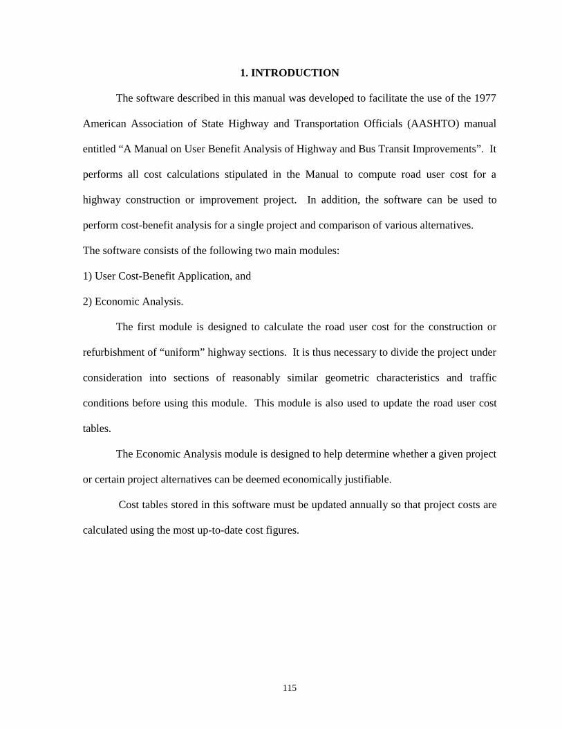
115
1. INTRODUCTION
The software described in this manual was developed to facilitate the use of the 1977
American Association of State Highway and Transportation Officials (AASHTO) manual
entitled “A Manual on User Benefit Analysis of Highway and Bus Transit Improvements”. It
performs all cost calculations stipulated in the Manual to compute road user cost for a
highway construction or improvement project. In addition, the software can be used to
perform cost-benefit analysis for a single project and comparison of various alternatives.
The software consists of the following two main modules:
1) User Cost-Benefit Application, and
2) Economic Analysis.
The first module is designed to calculate the road user cost for the construction or
refurbishment of “uniform” highway sections. It is thus necessary to divide the project under
consideration into sections of reasonably similar geometric characteristics and traffic
conditions before using this module. This module is also used to update the road user cost
tables.
The Economic Analysis module is designed to help determine whether a given project
or certain project alternatives can be deemed economically justifiable.
Cost tables stored in this software must be updated annually so that project costs are
calculated using the most up-to-date cost figures.
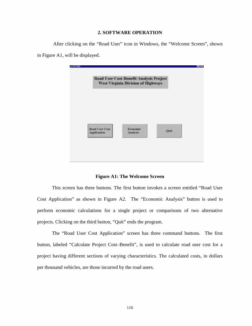
116
2. SOFTWARE OPERATION
After clicking on the “Road User” icon in Windows, the “Welcome Screen”, shown
in Figure A1, will be displayed.
Figure A1: The Welcome Screen
This screen has three buttons. The first button invokes a screen entitled “Road User
Cost Application” as shown in Figure A2. The “Economic Analysis” button is used to
perform economic calculations for a single project or comparisons of two alternative
projects. Clicking on the third button, “Quit” ends the program.
The “Road User Cost Application” screen has three command buttons. The first
button, labeled “Calculate Project Cost–Benefit”, is used to calculate road user cost for a
project having different sections of varying characteristics. The calculated costs, in dollars
per thousand vehicles, are those incurred by the road users.
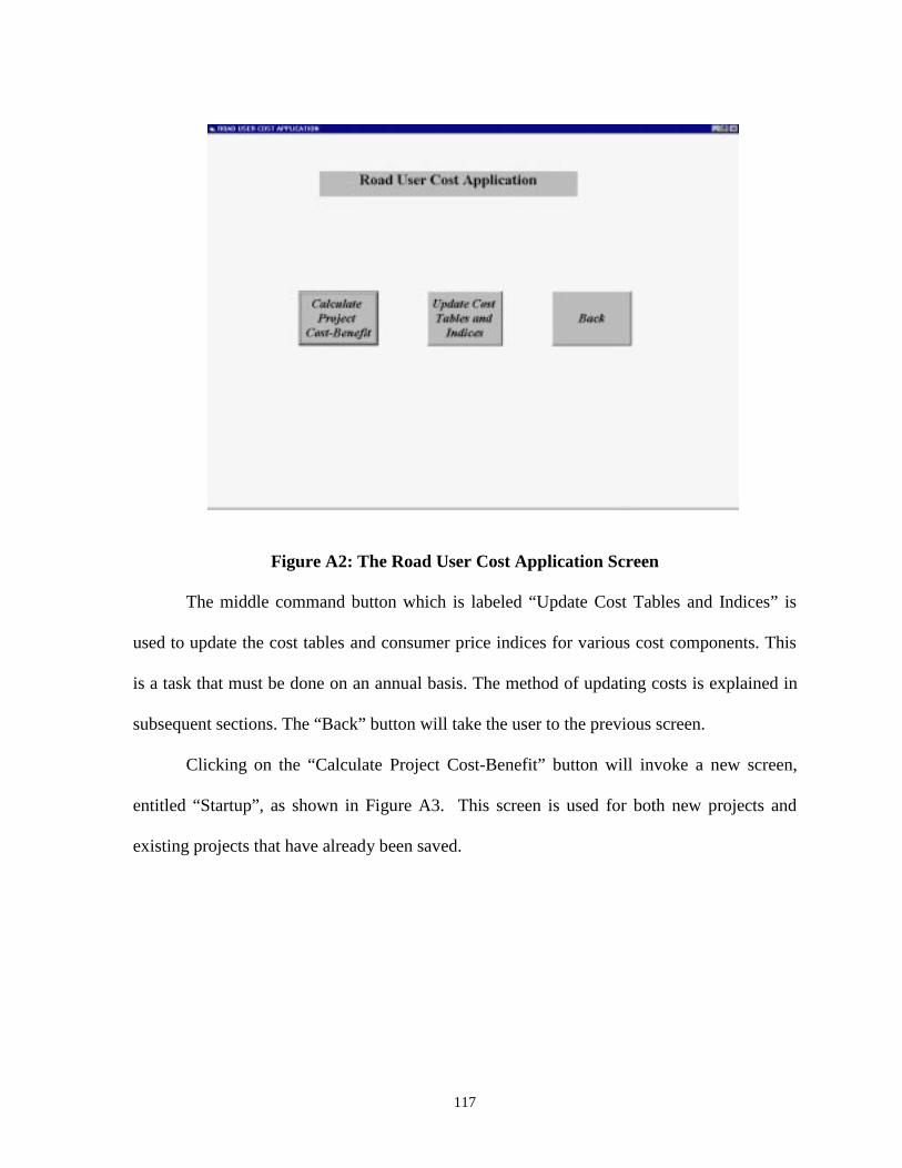
117
Figure A2: The Road User Cost Application Screen
The middle command button which is labeled “Update Cost Tables and Indices” is
used to update the cost tables and consumer price indices for various cost components. This
is a task that must be done on an annual basis. The method of updating costs is explained in
subsequent sections. The “Back” button will take the user to the previous screen.
Clicking on the “Calculate Project Cost-Benefit” button will invoke a new screen,
entitled “Startup”, as shown in Figure A3. This screen is used for both new projects and
existing projects that have already been saved.
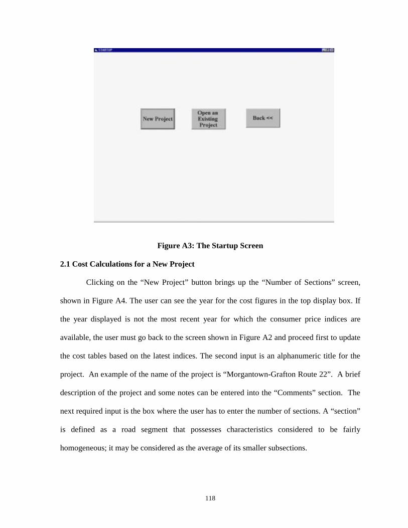
118
Figure A3: The Startup Screen
2.1 Cost Calculations for a New Project
Clicking on the “New Project” button brings up the “Number of Sections” screen,
shown in Figure A4. The user can see the year for the cost figures in the top display box. If
the year displayed is not the most recent year for which the consumer price indices are
available, the user must go back to the screen shown in Figure A2 and proceed first to update
the cost tables based on the latest indices. The second input is an alphanumeric title for the
project. An example of the name of the project is “Morgantown-Grafton Route 22”. A brief
description of the project and some notes can be entered into the “Comments” section. The
next required input is the box where the user has to enter the number of sections. A “section”
is defined as a road segment that possesses characteristics considered to be fairly
homogeneous; it may be considered as the average of its smaller subsections.
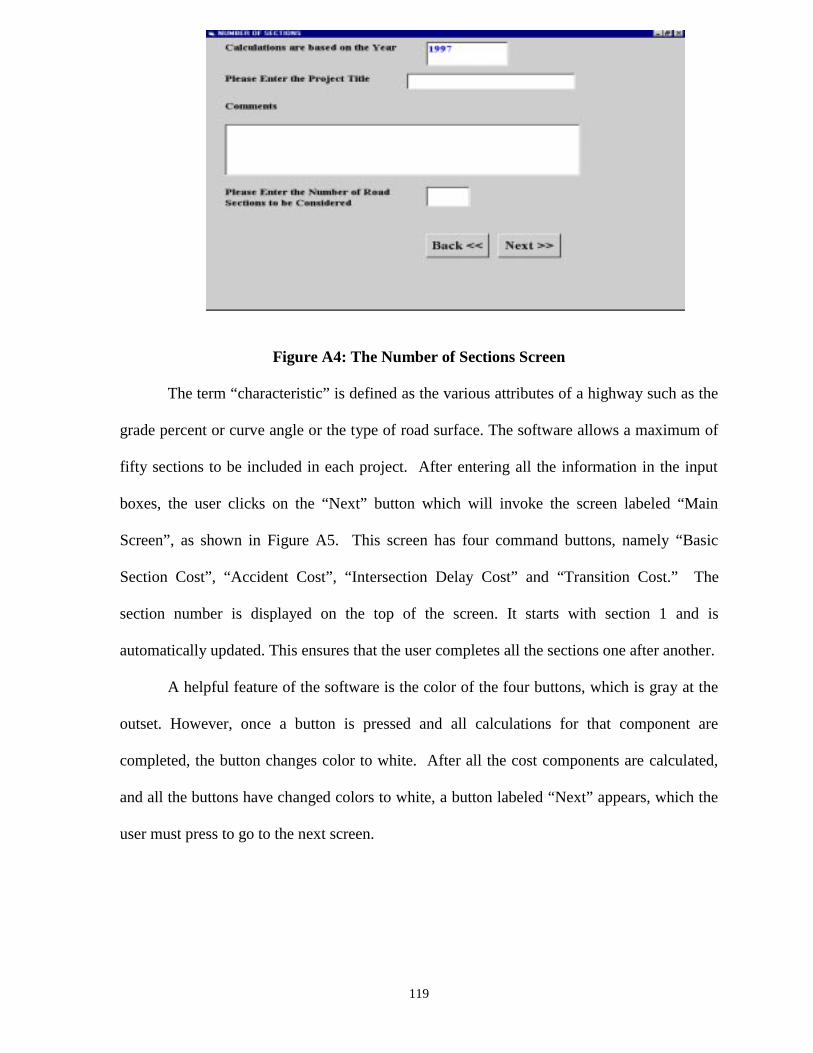
119
Figure A4: The Number of Sections Screen
The term “characteristic” is defined as the various attributes of a highway such as the
grade percent or curve angle or the type of road surface. The software allows a maximum of
fifty sections to be included in each project. After entering all the information in the input
boxes, the user clicks on the “Next” button which will invoke the screen labeled “Main
Screen”, as shown in Figure A5. This screen has four command buttons, namely “Basic
Section Cost”, “Accident Cost”, “Intersection Delay Cost” and “Transition Cost.” The
section number is displayed on the top of the screen. It starts with section 1 and is
automatically updated. This ensures that the user completes all the sections one after another.
A helpful feature of the software is the color of the four buttons, which is gray at the
outset. However, once a button is pressed and all calculations for that component are
completed, the button changes color to white. After all the cost components are calculated,
and all the buttons have changed colors to white, a button labeled “Next” appears, which the
user must press to go to the next screen.
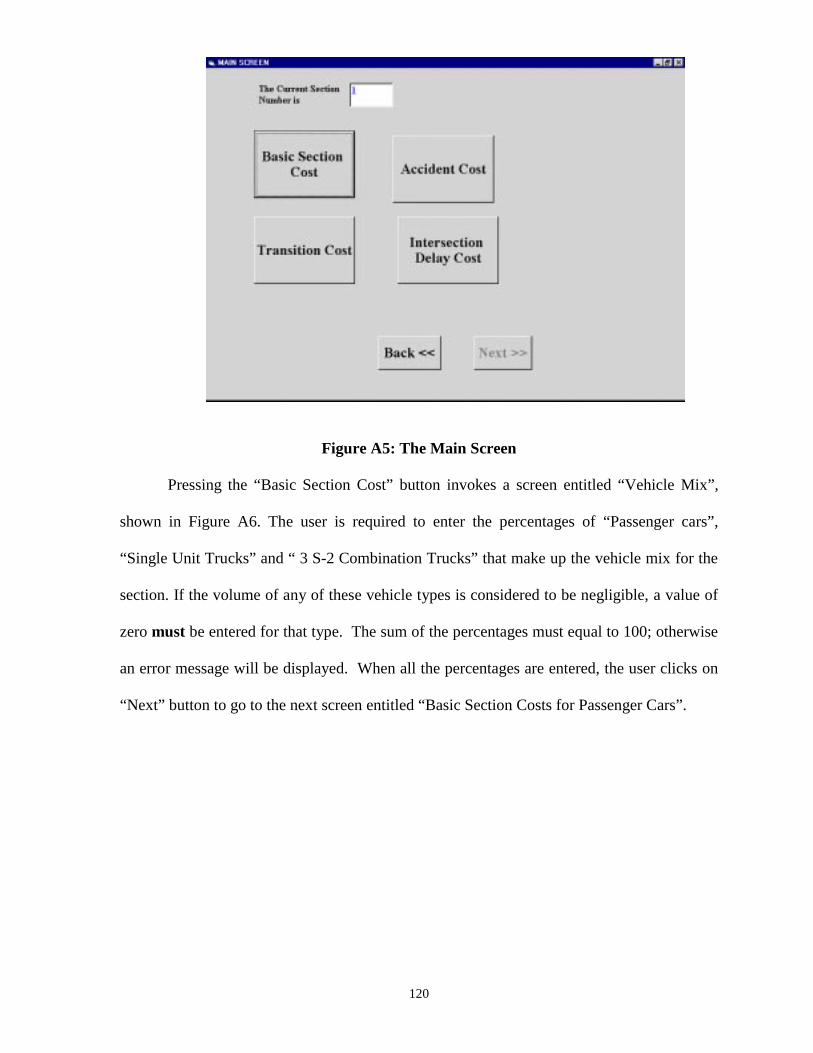
120
Figure A5: The Main Screen
Pressing the “Basic Section Cost” button invokes a screen entitled “Vehicle Mix”,
shown in Figure A6. The user is required to enter the percentages of “Passenger cars”,
“Single Unit Trucks” and “ 3 S-2 Combination Trucks” that make up the vehicle mix for the
section. If the volume of any of these vehicle types is considered to be negligible, a value of
zero must be entered for that type. The sum of the percentages must equal to 100; otherwise
an error message will be displayed. When all the percentages are entered, the user clicks on
“Next” button to go to the next screen entitled “Basic Section Costs for Passenger Cars”.
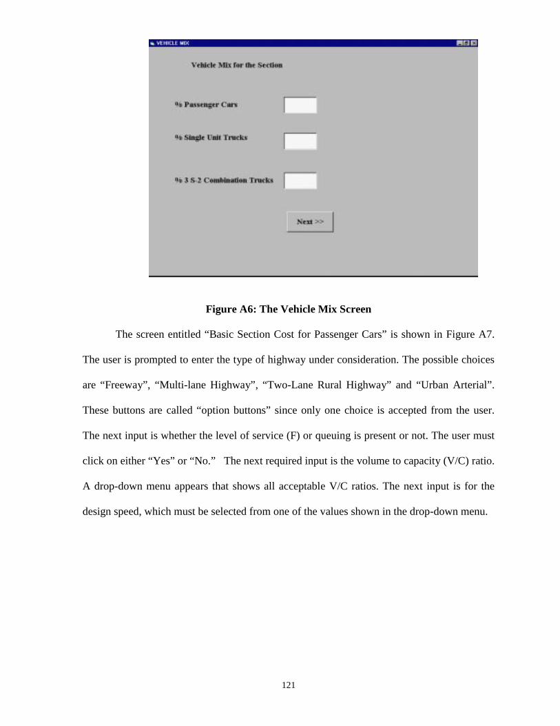
121
Figure A6: The Vehicle Mix Screen
The screen entitled “Basic Section Cost for Passenger Cars” is shown in Figure A7.
The user is prompted to enter the type of highway under consideration. The possible choices
are “Freeway”, “Multi-lane Highway”, “Two-Lane Rural Highway” and “Urban Arterial”.
These buttons are called “option buttons” since only one choice is accepted from the user.
The next input is whether the level of service (F) or queuing is present or not. The user must
click on either “Yes” or “No.” The next required input is the volume to capacity (V/C) ratio.
A drop-down menu appears that shows all acceptable V/C ratios. The next input is for the
design speed, which must be selected from one of the values shown in the drop-down menu.
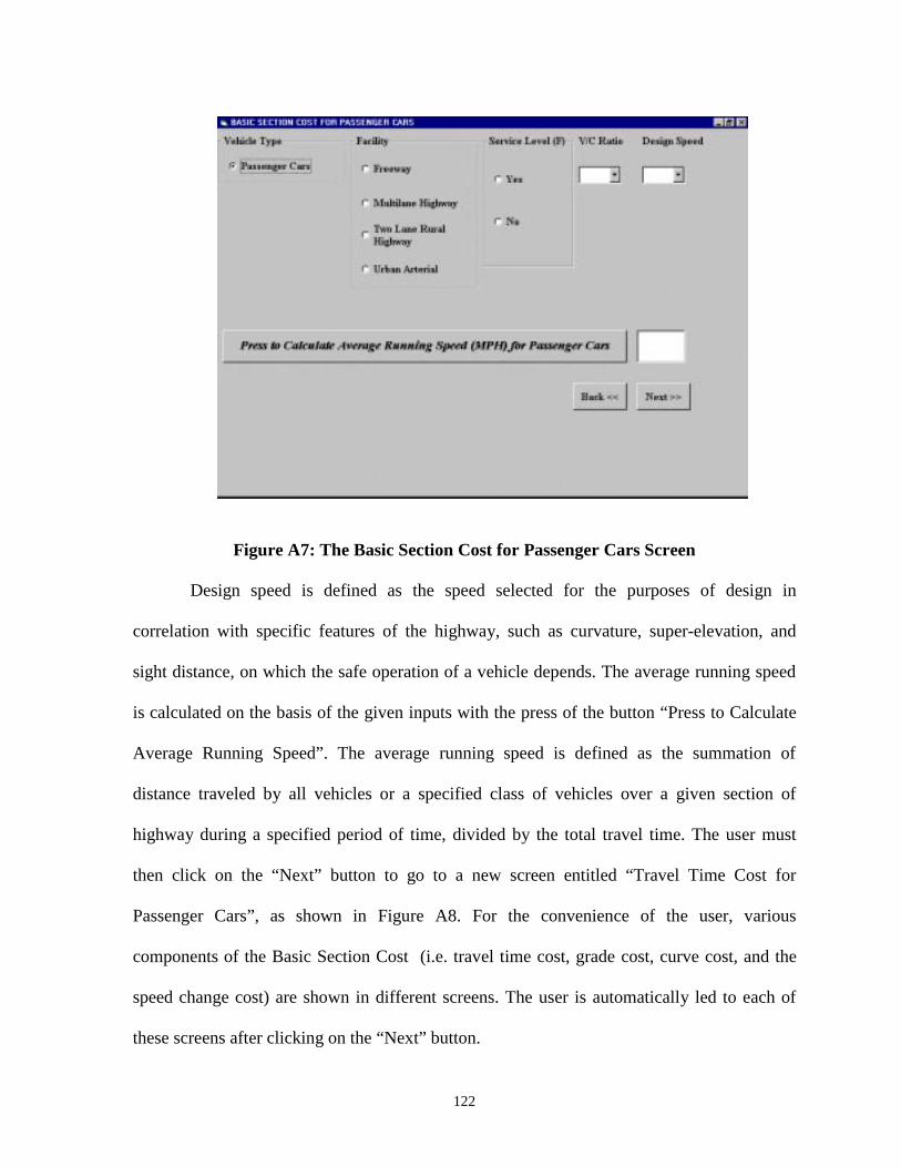
122
Figure A7: The Basic Section Cost for Passenger Cars Screen
Design speed is defined as the speed selected for the purposes of design in
correlation with specific features of the highway, such as curvature, super-elevation, and
sight distance, on which the safe operation of a vehicle depends. The average running speed
is calculated on the basis of the given inputs with the press of the button “Press to Calculate
Average Running Speed”. The average running speed is defined as the summation of
distance traveled by all vehicles or a specified class of vehicles over a given section of
highway during a specified period of time, divided by the total travel time. The user must
then click on the “Next” button to go to a new screen entitled “Travel Time Cost for
Passenger Cars”, as shown in Figure A8. For the convenience of the user, various
components of the Basic Section Cost (i.e. travel time cost, grade cost, curve cost, and the
speed change cost) are shown in different screens. The user is automatically led to each of
these screens after clicking on the “Next” button.
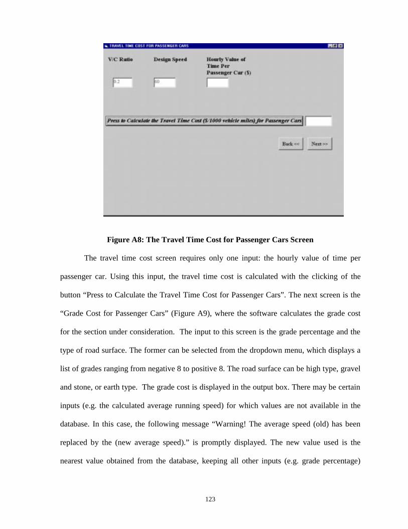
123
Figure A8: The Travel Time Cost for Passenger Cars Screen
The travel time cost screen requires only one input: the hourly value of time per
passenger car. Using this input, the travel time cost is calculated with the clicking of the
button “Press to Calculate the Travel Time Cost for Passenger Cars”. The next screen is the
“Grade Cost for Passenger Cars” (Figure A9), where the software calculates the grade cost
for the section under consideration. The input to this screen is the grade percentage and the
type of road surface. The former can be selected from the dropdown menu, which displays a
list of grades ranging from negative 8 to positive 8. The road surface can be high type, gravel
and stone, or earth type. The grade cost is displayed in the output box. There may be certain
inputs (e.g. the calculated average running speed) for which values are not available in the
database. In this case, the following message “Warning! The average speed (old) has been
replaced by the (new average speed).” is promptly displayed. The new value used is the
nearest value obtained from the database, keeping all other inputs (e.g. grade percentage)
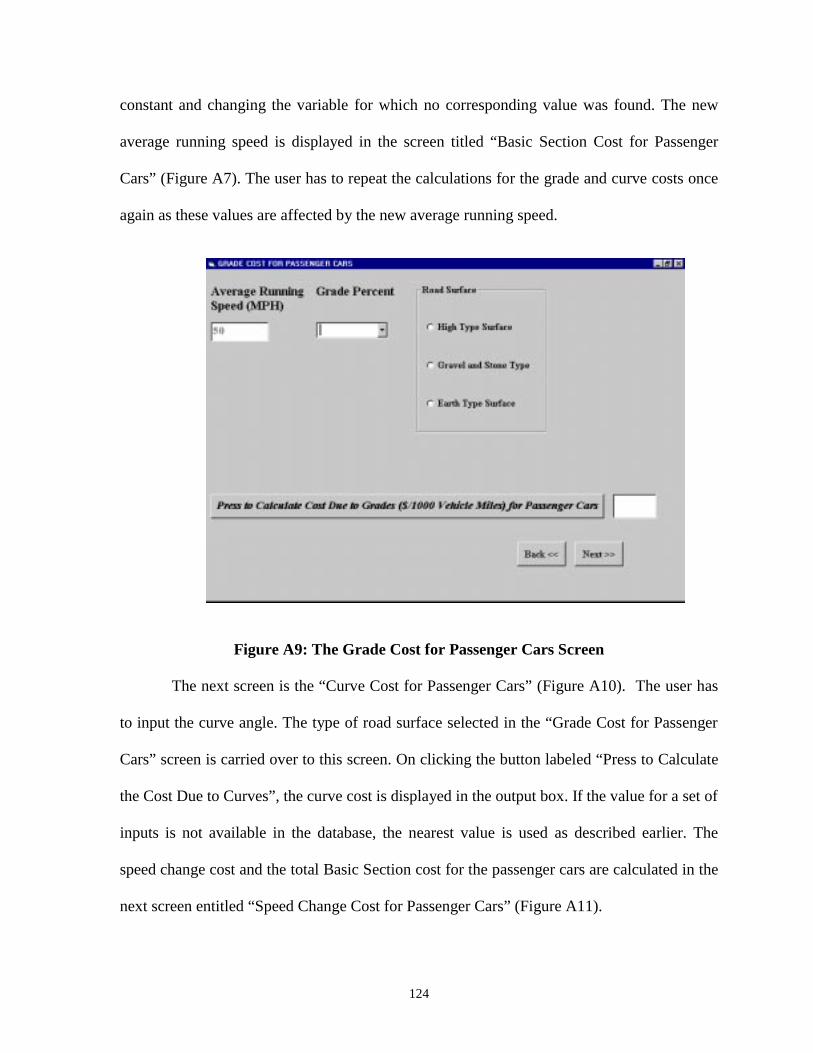
124
constant and changing the variable for which no corresponding value was found. The new
average running speed is displayed in the screen titled “Basic Section Cost for Passenger
Cars” (Figure A7). The user has to repeat the calculations for the grade and curve costs once
again as these values are affected by the new average running speed.
Figure A9: The Grade Cost for Passenger Cars Screen
The next screen is the “Curve Cost for Passenger Cars” (Figure A10). The user has
to input the curve angle. The type of road surface selected in the “Grade Cost for Passenger
Cars” screen is carried over to this screen. On clicking the button labeled “Press to Calculate
the Cost Due to Curves”, the curve cost is displayed in the output box. If the value for a set of
inputs is not available in the database, the nearest value is used as described earlier. The
speed change cost and the total Basic Section cost for the passenger cars are calculated in the
next screen entitled “Speed Change Cost for Passenger Cars” (Figure A11).
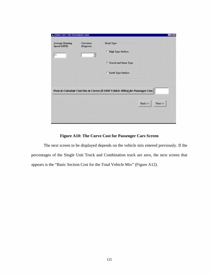
125
Figure A10: The Curve Cost for Passenger Cars Screen
The next screen to be displayed depends on the vehicle mix entered previously. If the
percentages of the Single Unit Truck and Combination truck are zero, the next screen that
appears is the “Basic Section Cost for the Total Vehicle Mix” (Figure A12).
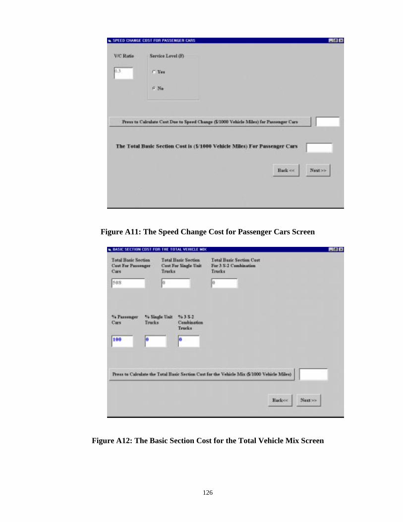
126
Figure A11: The Speed Change Cost for Passenger Cars Screen
Figure A12: The Basic Section Cost for the Total Vehicle Mix Screen
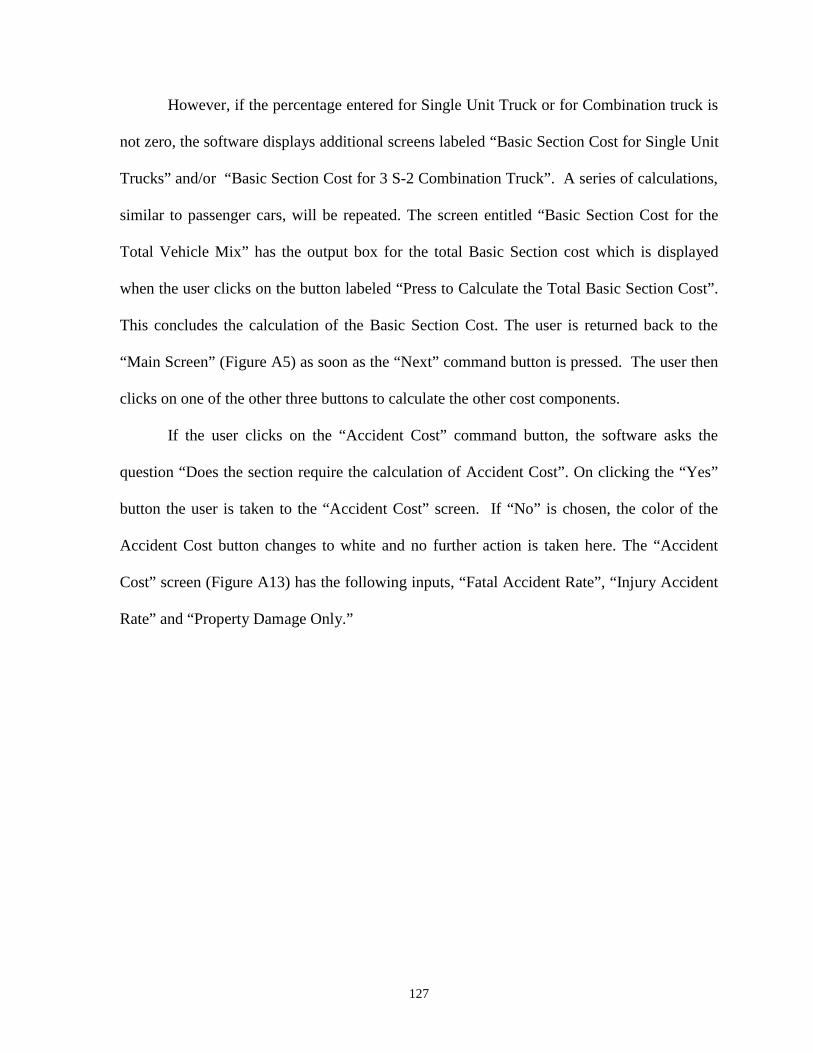
127
However, if the percentage entered for Single Unit Truck or for Combination truck is
not zero, the software displays additional screens labeled “Basic Section Cost for Single Unit
Trucks” and/or “Basic Section Cost for 3 S-2 Combination Truck”. A series of calculations,
similar to passenger cars, will be repeated. The screen entitled “Basic Section Cost for the
Total Vehicle Mix” has the output box for the total Basic Section cost which is displayed
when the user clicks on the button labeled “Press to Calculate the Total Basic Section Cost”.
This concludes the calculation of the Basic Section Cost. The user is returned back to the
“Main Screen” (Figure A5) as soon as the “Next” command button is pressed. The user then
clicks on one of the other three buttons to calculate the other cost components.
If the user clicks on the “Accident Cost” command button, the software asks the
question “Does the section require the calculation of Accident Cost”. On clicking the “Yes”
button the user is taken to the “Accident Cost” screen. If “No” is chosen, the color of the
Accident Cost button changes to white and no further action is taken here. The “Accident
Cost” screen (Figure A13) has the following inputs, “Fatal Accident Rate”, “Injury Accident
Rate” and “Property Damage Only.”
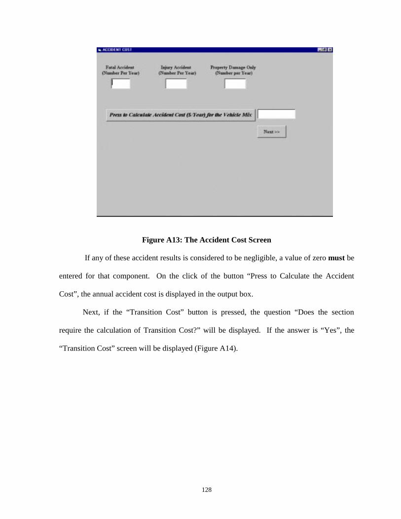
128
Figure A13: The Accident Cost Screen
If any of these accident results is considered to be negligible, a value of zero must be
entered for that component. On the click of the button “Press to Calculate the Accident
Cost”, the annual accident cost is displayed in the output box.
Next, if the “Transition Cost” button is pressed, the question “Does the section
require the calculation of Transition Cost?” will be displayed. If the answer is “Yes”, the
“Transition Cost” screen will be displayed (Figure A14).
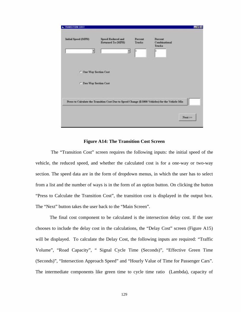
129
Figure A14: The Transition Cost Screen
The “Transition Cost” screen requires the following inputs: the initial speed of the
vehicle, the reduced speed, and whether the calculated cost is for a one-way or two-way
section. The speed data are in the form of dropdown menus, in which the user has to select
from a list and the number of ways is in the form of an option button. On clicking the button
“Press to Calculate the Transition Cost”, the transition cost is displayed in the output box.
The “Next” button takes the user back to the “Main Screen”.
The final cost component to be calculated is the intersection delay cost. If the user
chooses to include the delay cost in the calculations, the “Delay Cost” screen (Figure A15)
will be displayed. To calculate the Delay Cost, the following inputs are required: “Traffic
Volume”, “Road Capacity”, “ Signal Cycle Time (Seconds)”, “Effective Green Time
(Seconds)”, “Intersection Approach Speed” and “Hourly Value of Time for Passenger Cars”.
The intermediate components like green time to cycle time ratio (Lambda), capacity of
130
approach and the volume to capacity ratio of approach are calculated on the click of the
button labeled “Press to Calculate the Delay Cost”.
Figure A15: The Intersection Delay Cost Due to Stopping Screen
The next screen is entitled “Intersection Delay Cost due to Idling” (Figure A16)
where the idling cost is computed. The input data are the same as for the Delay Costs and are
displayed here for the user’s information. The user needs to enter only the “Number of
Intersections”. The Total Intersection Cost (Delay Cost + Idling Cost) is calculated and
displayed in this screen. The user then goes back to the “Main Screen.” If at this time the
color of all four buttons has changed to white, the “Next” button will appear on the Main
Screen. This button leads to the screen labeled “Total Cost” (Figure A17), where all the costs
calculated so far is displayed. The user is now required to enter the length of the section (in
miles). The total cost is displayed as soon as the button “Press to Calculate the Total Cost” is
clicked.
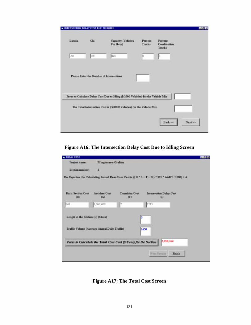
131
Figure A16: The Intersection Delay Cost Due to Idling Screen
Figure A17: The Total Cost Screen
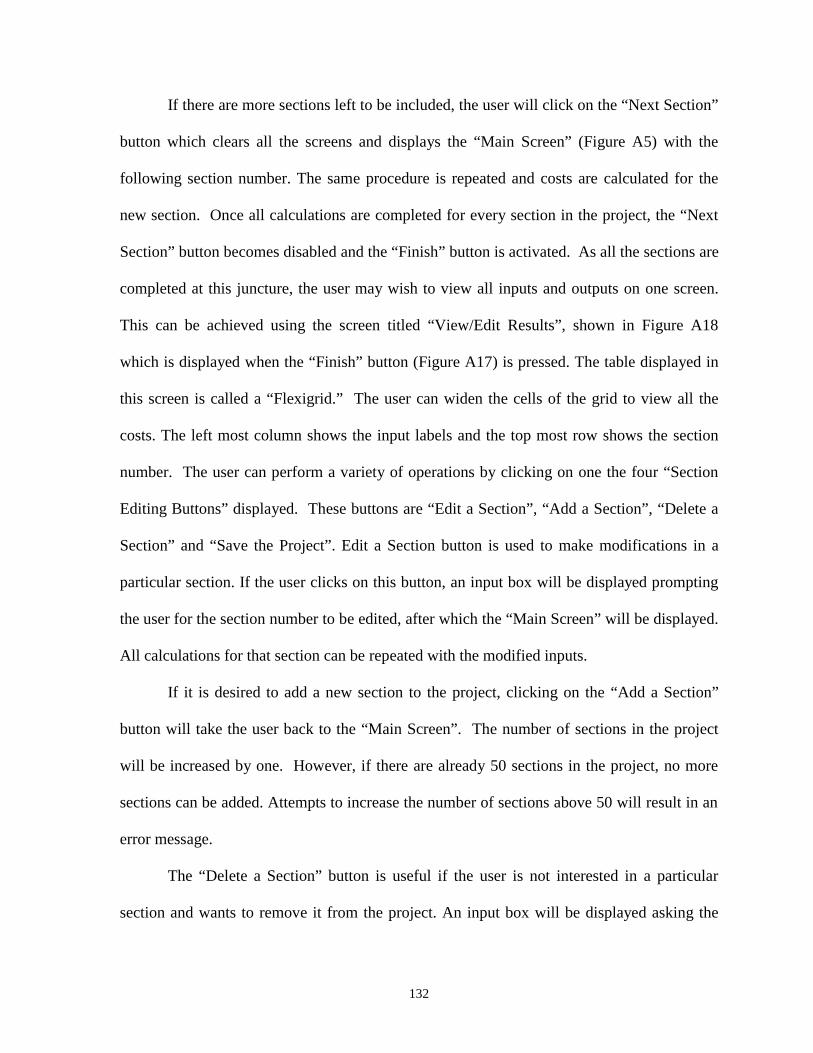
132
If there are more sections left to be included, the user will click on the “Next Section”
button which clears all the screens and displays the “Main Screen” (Figure A5) with the
following section number. The same procedure is repeated and costs are calculated for the
new section. Once all calculations are completed for every section in the project, the “Next
Section” button becomes disabled and the “Finish” button is activated. As all the sections are
completed at this juncture, the user may wish to view all inputs and outputs on one screen.
This can be achieved using the screen titled “View/Edit Results”, shown in Figure A18
which is displayed when the “Finish” button (Figure A17) is pressed. The table displayed in
this screen is called a “Flexigrid.” The user can widen the cells of the grid to view all the
costs. The left most column shows the input labels and the top most row shows the section
number. The user can perform a variety of operations by clicking on one the four “Section
Editing Buttons” displayed. These buttons are “Edit a Section”, “Add a Section”, “Delete a
Section” and “Save the Project”. Edit a Section button is used to make modifications in a
particular section. If the user clicks on this button, an input box will be displayed prompting
the user for the section number to be edited, after which the “Main Screen” will be displayed.
All calculations for that section can be repeated with the modified inputs.
If it is desired to add a new section to the project, clicking on the “Add a Section”
button will take the user back to the “Main Screen”. The number of sections in the project
will be increased by one. However, if there are already 50 sections in the project, no more
sections can be added. Attempts to increase the number of sections above 50 will result in an
error message.
The “Delete a Section” button is useful if the user is not interested in a particular
section and wants to remove it from the project. An input box will be displayed asking the
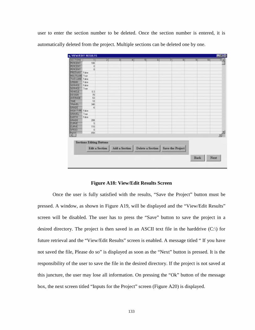
133
user to enter the section number to be deleted. Once the section number is entered, it is
automatically deleted from the project. Multiple sections can be deleted one by one.
Figure A18: View/Edit Results Screen
Once the user is fully satisfied with the results, “Save the Project” button must be
pressed. A window, as shown in Figure A19, will be displayed and the “View/Edit Results”
screen will be disabled. The user has to press the “Save” button to save the project in a
desired directory. The project is then saved in an ASCII text file in the harddrive (C:\) for
future retrieval and the “View/Edit Results” screen is enabled. A message titled “ If you have
not saved the file, Please do so” is displayed as soon as the “Next” button is pressed. It is the
responsibility of the user to save the file in the desired directory. If the project is not saved at
this juncture, the user may lose all information. On pressing the “Ok” button of the message
box, the next screen titled “Inputs for the Project” screen (Figure A20) is displayed.
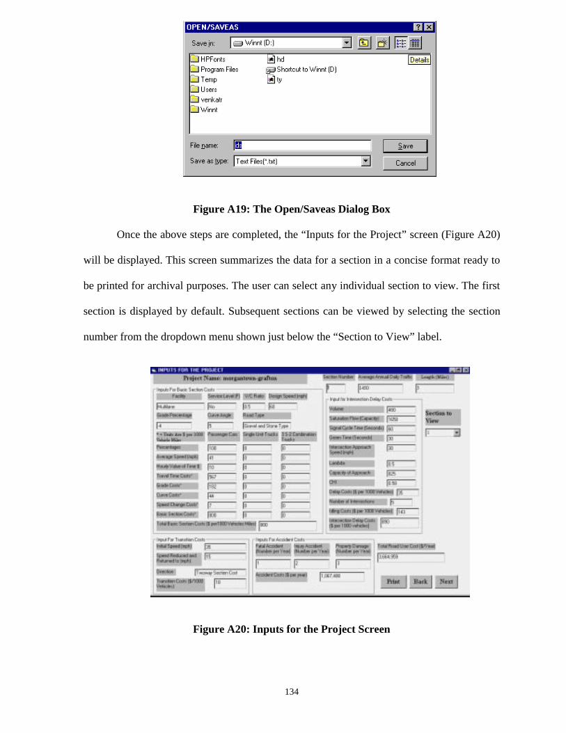
134
Figure A19: The Open/Saveas Dialog Box
Once the above steps are completed, the “Inputs for the Project” screen (Figure A20)
will be displayed. This screen summarizes the data for a section in a concise format ready to
be printed for archival purposes. The user can select any individual section to view. The first
section is displayed by default. Subsequent sections can be viewed by selecting the section
number from the dropdown menu shown just below the “Section to View” label.
Figure A20: Inputs for the Project Screen
135
He can also take printouts of the inputs by simply pressing the “Print” button. On
clicking the “Print” button, a window titled “Print Results” is displayed as shown in Figure
A21.
Figure A21: The Print Results Screen
The user has to select a section number to print. He can print individual sections by
selecting a particular section number from the dropdown titled “ Select Section Number to be
Printed” or select “All” from the dropdown to print all sections in succession. Each section
will be printed on a separate page.
Clicking on the “Next” button in Figure A20 will take the user to the “View Results”
screen (Figure A22). This screen displays all the cost components of each section (ten
sections per screen) and the total costs for the whole project. At this point the user can print
the results for future reference.

136
Figure A22: The View Results Screen
The “Back” button helps the user go back to the previous screen. The “Next” button
helps the user to move to the next screen in case there are more than ten sections. Otherwise,
the “Next” button is replaced by the “End” button, which helps the user to exit the software.
On pressing the “End” button, a window appears with a message “Do you want to go to a
New Session?”. If the user presses the “Yes” button, the screen in Figure A1 appears. The
“No” button terminates the software.
2.2 Opening an Existing File
To retrieve information saved in an existing file, the user must click on the “Opening
an Existing File” button displayed in the “Startup” screen (Figure A3). This would bring up
the open/saveas dialog box similar to that shown in Figure A19 from which the user selects
the file to open. The user can also browse through all directories to find the desired file.
137
Once a file is selected, a new screen entitled “Opening an Existing File” (Figure A23) will be
displayed. This screen shows the file name, the title of the project, brief comments on the
project and the number of sections. An input box is also shown prompting the user for the
section number to be viewed or edited. If the value entered for the section number to be
viewed is larger than the number of sections in the project, an error message will be
displayed.
Figure A23: Opening an Existing File Screen
The user must enter a valid section number and press the “Ok” button to proceed to
the “Main Screen”. A label on top of the screen shows the section number being viewed.
The “Basic Section Cost”, “Accident Cost”, “Intersection Delay Cost” and “Transition Cost”
buttons are displayed on the screen. The user may press any one of them to view or make
changes to the cost components.
138
Due to the fact that change in inputs in one screen may affect other screens, the user
has to make sure that changes are reflected in all the required screens. If the user fails to do
so, error messages will be displayed. As an example, if the user wants to change the grade
percentage for passenger cars, he has to go to the “Grade Cost for Passenger Car” screen,
select a new grade percentage from the dropdown menu and click on the button “Press to
Calculate Grade Cost” to complete the calculation. The new grade cost also changes the total
Basic Section cost, so the user has to proceed to the “Speed Change Cost for Passenger Cars”
screen and click on “Press to Calculate the Speed Change Cost” to display the changed cost.
Once all the necessary changes are made, the user clicks the “Next” button on the
“Main Screen” to move to the “Total Cost” screen. Here, the new costs are displayed in their
respective output boxes. At this point it is also possible to change the length of the section.
When the user is satisfied with the changes, the button “Press to Calculate the Total Cost for
the Section” must be pressed to display the new total cost.
The user can go to the next screen titled “View/Edit Results” (Figure A18) where it is
possible to use the various editing buttons available. The old costs may be revised either by
viewing each section as in the screen “Opening an Existing File” (Figure A23) or by using
the edit buttons in the screen “View/Edit Results” (Figure A18). After making all the
changes needed, the user must save all the work for future retrieval. The user can proceed to
obtain printouts of the projects after changes.
2.3 Updating Cost Tables
All cost tables are stored in Excel worksheets. These tables must be updated annually
so that calculated costs reflect the latest cost figures. The first step is to press the ”Update
139
Cost Tables and Indices” button on the “Road User Cost Application” screen, shown in
Figure A2. Once this button is clicked, screen entitled “View/Update Indices” (Figure A24)
is invoked. This screen opens and displays the base year and consumer price indices (CPI)
for all price components: CPI (Fuel), CPI (Motor Oil), CPI (Depreciation), CPI (Tires) and
CPI Maintenance) and the latest producer price indices (PPI), previously called wholesale
price indices like PPI (Fuel, Single Unit Truck), PPI (Fuel, Combination Truck), PPI (Motor
Oil), PPI (Depreciation, Single Unit Truck), PPI (Depreciation, Combination Truck), PPI
(Tires), CPI (Total) and WPI (Industrial Commodities) The user must enter the current year
and the latest CPI’s and PPI’s in the specified input boxes and click the “Save Changes and
Update Cost Tables” button to update all the tables.
The latest available vehicular accident costs, as published by the National Safety
Council, must also be entered. Once the updating is finished, the user goes back to the “Road
User Cost Application” screen. If the user is not interested in any modifications, he can go
back to the “Road User Cost Application” screen by pressing the “Back (No Modifications) ”
button.
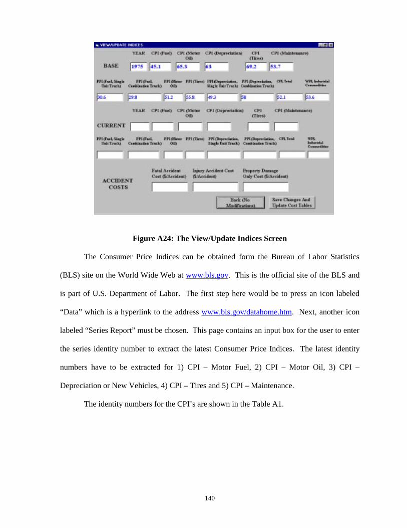
140
Figure A24: The View/Update Indices Screen
The Consumer Price Indices can be obtained form the Bureau of Labor Statistics
(BLS) site on the World Wide Web at www.bls.gov. This is the official site of the BLS and
is part of U.S. Department of Labor. The first step here would be to press an icon labeled
“Data” which is a hyperlink to the address www.bls.gov/datahome.htm. Next, another icon
labeled “Series Report” must be chosen. This page contains an input box for the user to enter
the series identity number to extract the latest Consumer Price Indices. The latest identity
numbers have to be extracted for 1) CPI – Motor Fuel, 2) CPI – Motor Oil, 3) CPI –
Depreciation or New Vehicles, 4) CPI – Tires and 5) CPI – Maintenance.
The identity numbers for the CPI’s are shown in the Table A1.
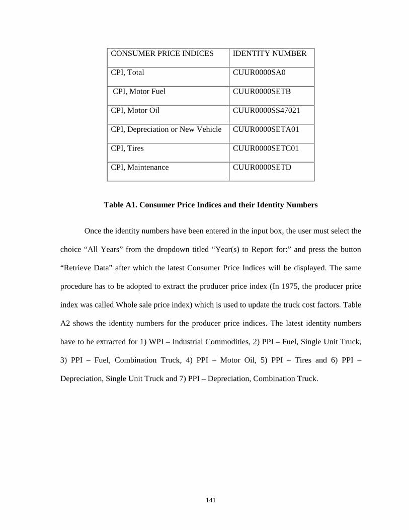
141
CONSUMER PRICE INDICES IDENTITY NUMBER
CPI, Total CUUR0000SA0
CPI, Motor Fuel CUUR0000SETB
CPI, Motor Oil CUUR0000SS47021
CPI, Depreciation or New Vehicle CUUR0000SETA01
CPI, Tires CUUR0000SETC01
CPI, Maintenance CUUR0000SETD
Table A1. Consumer Price Indices and their Identity Numbers
Once the identity numbers have been entered in the input box, the user must select the
choice “All Years” from the dropdown titled “Year(s) to Report for:” and press the button
“Retrieve Data” after which the latest Consumer Price Indices will be displayed. The same
procedure has to be adopted to extract the producer price index (In 1975, the producer price
index was called Whole sale price index) which is used to update the truck cost factors. Table
A2 shows the identity numbers for the producer price indices. The latest identity numbers
have to be extracted for 1) WPI – Industrial Commodities, 2) PPI – Fuel, Single Unit Truck,
3) PPI – Fuel, Combination Truck, 4) PPI – Motor Oil, 5) PPI – Tires and 6) PPI –
Depreciation, Single Unit Truck and 7) PPI – Depreciation, Combination Truck.
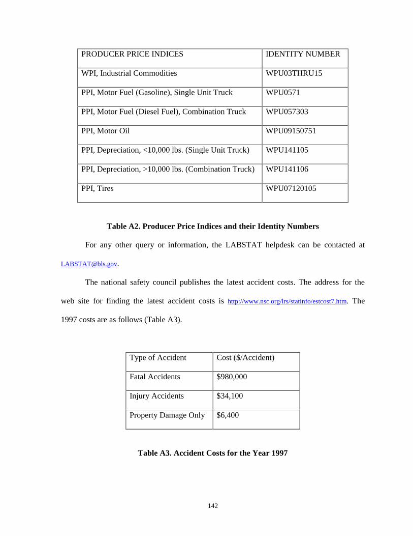
142
PRODUCER PRICE INDICES IDENTITY NUMBER
WPI, Industrial Commodities WPU03THRU15
PPI, Motor Fuel (Gasoline), Single Unit Truck WPU0571
PPI, Motor Fuel (Diesel Fuel), Combination Truck WPU057303
PPI, Motor Oil WPU09150751
PPI, Depreciation, <10,000 lbs. (Single Unit Truck) WPU141105
PPI, Depreciation, >10,000 lbs. (Combination Truck) WPU141106
PPI, Tires WPU07120105
Table A2. Producer Price Indices and their Identity Numbers
For any other query or information, the LABSTAT helpdesk can be contacted at
The national safety council publishes the latest accident costs. The address for the
web site for finding the latest accident costs is http://www.nsc.org/lrs/statinfo/estcost7.htm. The
1997 costs are as follows (Table A3).
Type of Accident Cost ($/Accident)
Fatal Accidents $980,000
Injury Accidents $34,100
Property Damage Only $6,400
Table A3. Accident Costs for the Year 1997
143
2.4 Economic Analysis
Another application of the software is to compute the present value of all the annual
user benefits due to the improvement over the analysis period, and to compare this present
value with the computed present value of the project costs associated with the improvement.
A project (or project alternative) can be deemed economically justifiable if the present value
of the project-related benefits exceeds the present value of all project-related costs. The user
clicks on the Button “Economic Analysis” displayed in the “Welcome” screen (Figure A1),
to invoke the “Economic Analysis” screen, shown in Figure A25, which includes three
buttons.
The “Net Present Value for Project with Constant Growth” button is used to calculate
the present value for a project that has a constant anticipated annual growth rate for
maintenance and user costs during the analysis period. On clicking this button, the screen
entitled “Economic analysis for Uniform Increase or Decrease” (Figure A26) will be
displayed.
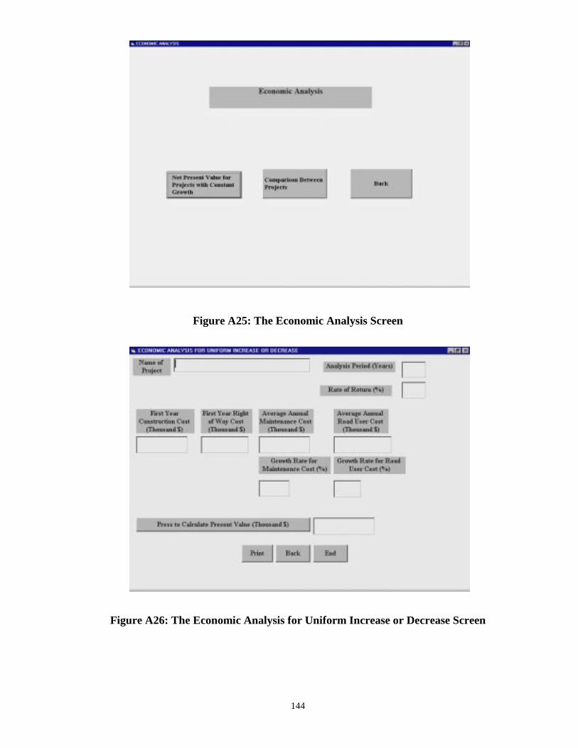
144
Figure A25: The Economic Analysis Screen
Figure A26: The Economic Analysis for Uniform Increase or Decrease Screen
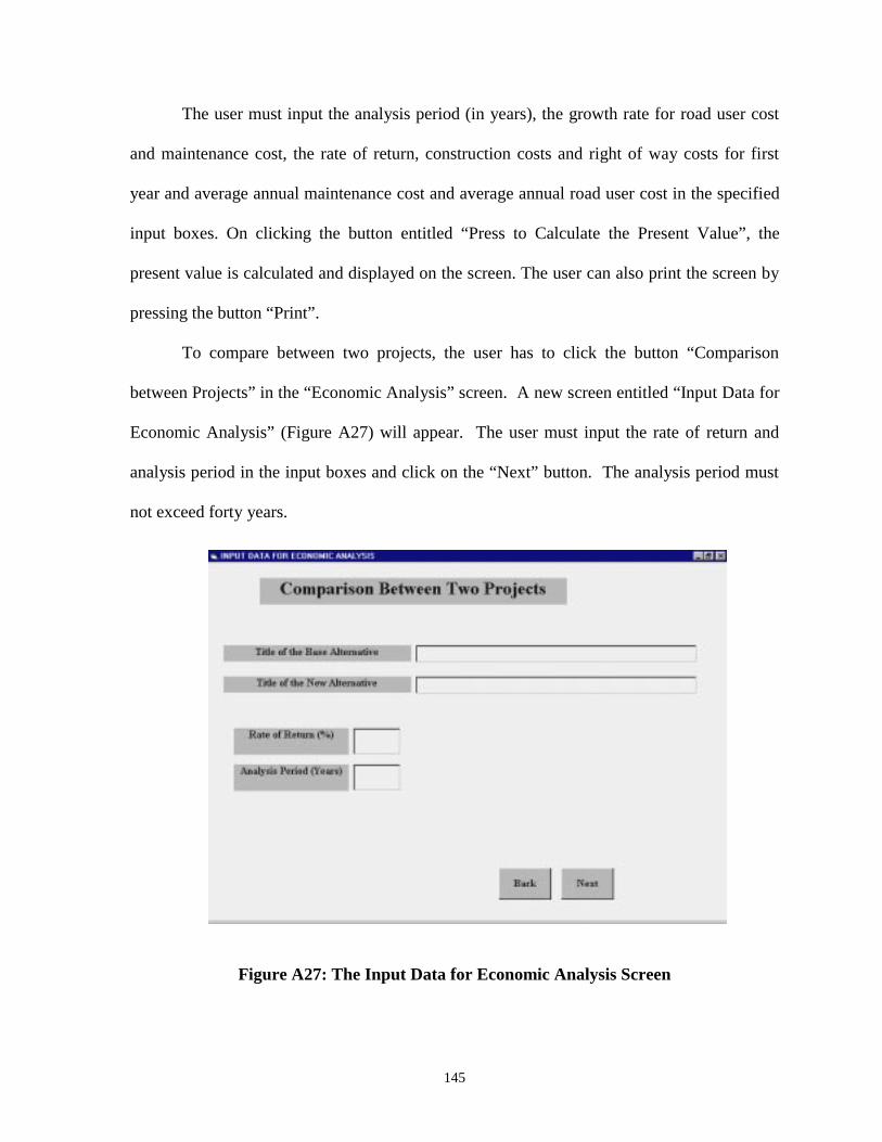
145
The user must input the analysis period (in years), the growth rate for road user cost
and maintenance cost, the rate of return, construction costs and right of way costs for first
year and average annual maintenance cost and average annual road user cost in the specified
input boxes. On clicking the button entitled “Press to Calculate the Present Value”, the
present value is calculated and displayed on the screen. The user can also print the screen by
pressing the button “Print”.
To compare between two projects, the user has to click the button “Comparison
between Projects” in the “Economic Analysis” screen. A new screen entitled “Input Data for
Economic Analysis” (Figure A27) will appear. The user must input the rate of return and
analysis period in the input boxes and click on the “Next” button. The analysis period must
not exceed forty years.
Figure A27: The Input Data for Economic Analysis Screen
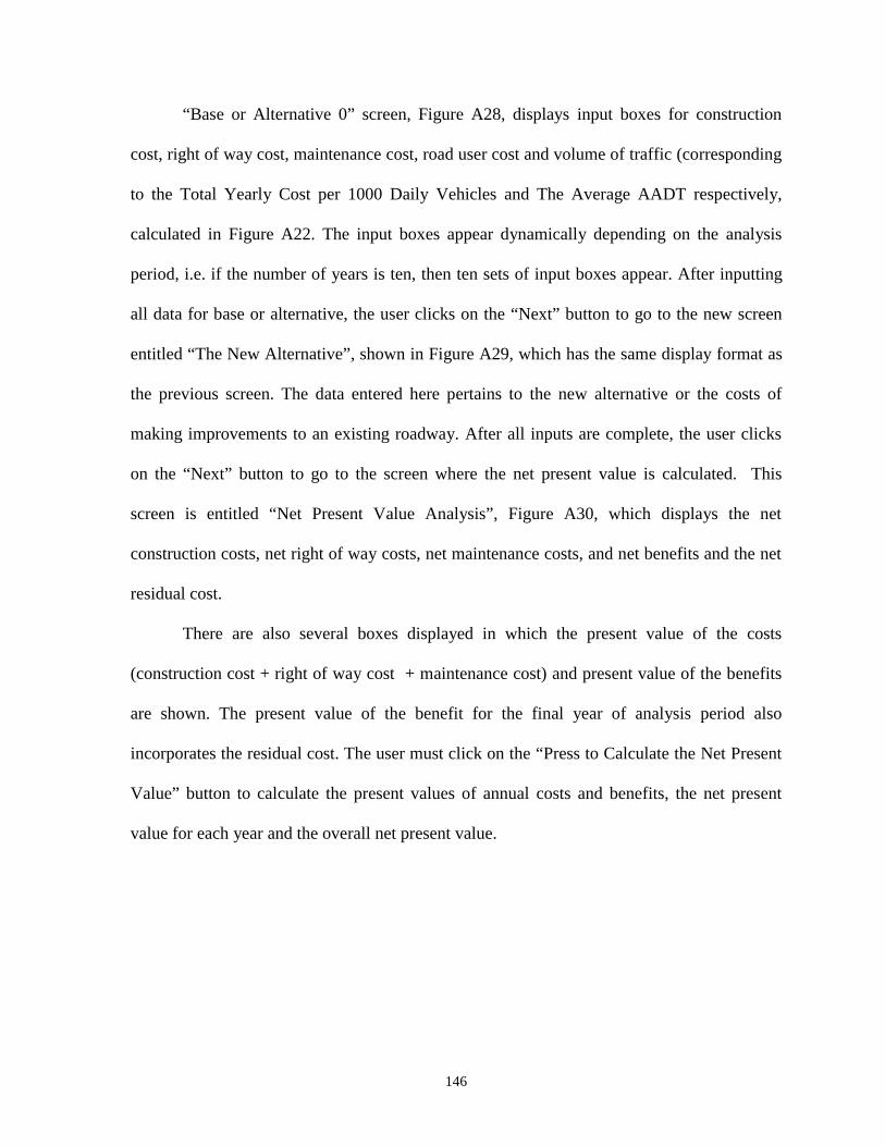
146
“Base or Alternative 0” screen, Figure A28, displays input boxes for construction
cost, right of way cost, maintenance cost, road user cost and volume of traffic (corresponding
to the Total Yearly Cost per 1000 Daily Vehicles and The Average AADT respectively,
calculated in Figure A22. The input boxes appear dynamically depending on the analysis
period, i.e. if the number of years is ten, then ten sets of input boxes appear. After inputting
all data for base or alternative, the user clicks on the “Next” button to go to the new screen
entitled “The New Alternative”, shown in Figure A29, which has the same display format as
the previous screen. The data entered here pertains to the new alternative or the costs of
making improvements to an existing roadway. After all inputs are complete, the user clicks
on the “Next” button to go to the screen where the net present value is calculated. This
screen is entitled “Net Present Value Analysis”, Figure A30, which displays the net
construction costs, net right of way costs, net maintenance costs, and net benefits and the net
residual cost.
There are also several boxes displayed in which the present value of the costs
(construction cost + right of way cost + maintenance cost) and present value of the benefits
are shown. The present value of the benefit for the final year of analysis period also
incorporates the residual cost. The user must click on the “Press to Calculate the Net Present
Value” button to calculate the present values of annual costs and benefits, the net present
value for each year and the overall net present value.
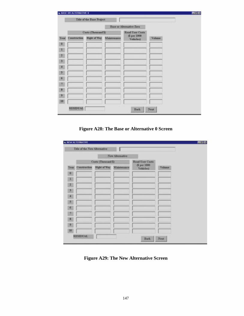
147
Figure A28: The Base or Alternative 0 Screen
Figure A29: The New Alternative Screen
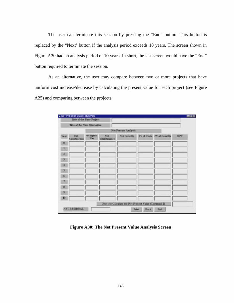
148
The user can terminate this session by pressing the “End” button. This button is
replaced by the “Next’ button if the analysis period exceeds 10 years. The screen shown in
Figure A30 had an analysis period of 10 years. In short, the last screen would have the “End”
button required to terminate the session.
As an alternative, the user may compare between two or more projects that have
uniform cost increase/decrease by calculating the present value for each project (see Figure
A25) and comparing between the projects.
Figure A30: The Net Present Value Analysis Screen
149
3. Valid Ranges for Inputs and Parameters
User inputs have to be consistent and valid for the proper functioning of the software.
Also, calculations can be completed only if all the inputs are entered. Several display and
error messages are designed to alert the user in case of missing or inconstitent inputs. In the
following, a number of possible inconsistencies are discussed.
In most cases, the user is required to enter a value for a variable or choose from a drop-down
menu. If the value entered is not included in the drop-down menu, the software will not
respond. For example, valid choices for the design speed for a freeway is 70 miles per hour,
60 miles per hour and 50 miles per hour. A speed other than the above-mentioned values,
such as 65 miles per hour, will result in the software not responding to the input. Another
example is the user input for vehicle to capacity ratio. It has a range form 0 to 1 in steps of
0.1 increase. An input of 0.25 is considered inconstitent.
A different type of inconsistent input may occur when calculating intersection delay
costs. A number of intermediate values are calculated like lambda (Ratio of Green Time to
Signal Cycle Time), Capacity of Approach (Lambda * Saturation Flow or Capacity) and chi
(Volume / Capacity of Approach). The value of lambda must be between 0.2 and 0.8. The
value of capacity of approach is between 200 and 4,400. The value of chi is between 0.1 and
0.8. Intersection approach speed is between 5 to 55 miles per hour.
The software also assumes that percentage of cars is greater than zero for every
section of a project. An input of zero percent for cars will result in an error message to be
displayed.
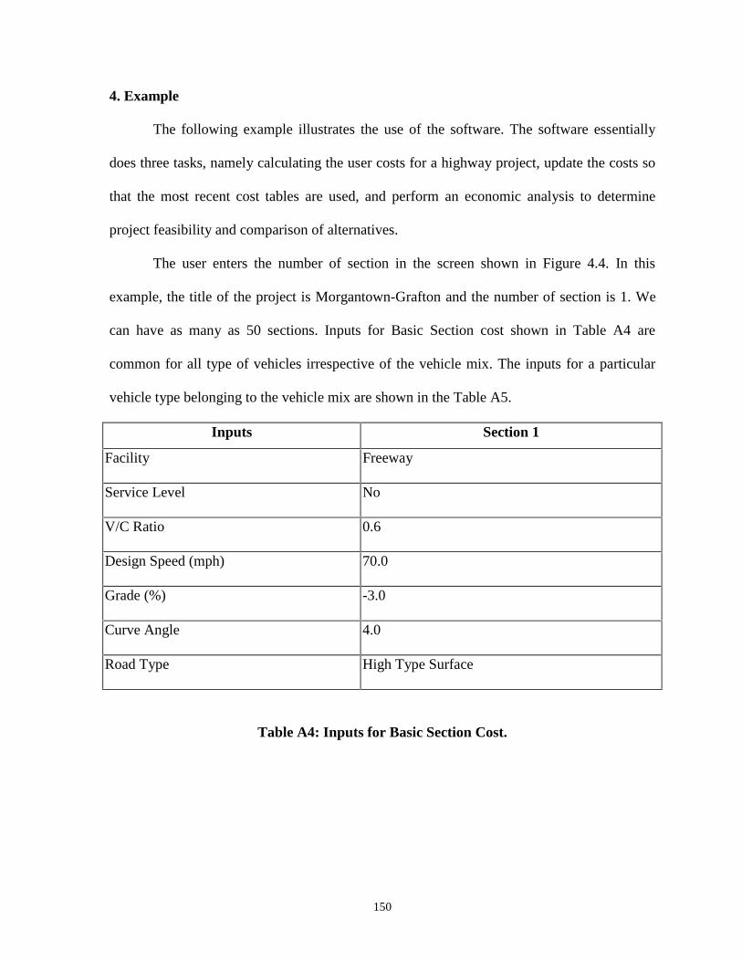
150
4. Example
The following example illustrates the use of the software. The software essentially
does three tasks, namely calculating the user costs for a highway project, update the costs so
that the most recent cost tables are used, and perform an economic analysis to determine
project feasibility and comparison of alternatives.
The user enters the number of section in the screen shown in Figure 4.4. In this
example, the title of the project is Morgantown-Grafton and the number of section is 1. We
can have as many as 50 sections. Inputs for Basic Section cost shown in Table A4 are
common for all type of vehicles irrespective of the vehicle mix. The inputs for a particular
vehicle type belonging to the vehicle mix are shown in the Table A5.
Inputs Section 1
Facility Freeway
Service Level No
V/C Ratio 0.6
Design Speed (mph) 70.0
Grade (%) -3.0
Curve Angle 4.0
Road Type High Type Surface
Table A4: Inputs for Basic Section Cost.
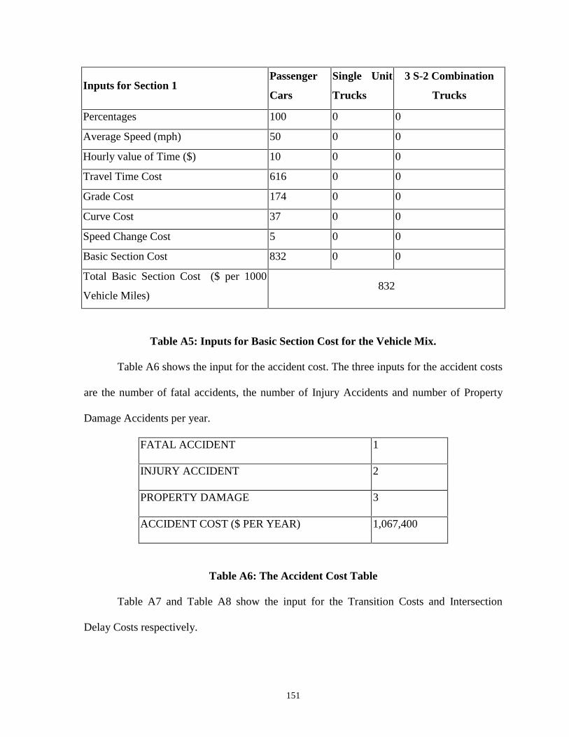
151
Inputs for Section 1Passenger
Cars
Single Unit
Trucks
3 S-2 Combination
Trucks
Percentages 100 0 0
Average Speed (mph) 50 0 0
Hourly value of Time ($) 10 0 0
Travel Time Cost 616 0 0
Grade Cost 174 0 0
Curve Cost 37 0 0
Speed Change Cost 5 0 0
Basic Section Cost 832 0 0
Total Basic Section Cost ($ per 1000
Vehicle Miles)832
Table A5: Inputs for Basic Section Cost for the Vehicle Mix.
Table A6 shows the input for the accident cost. The three inputs for the accident costs
are the number of fatal accidents, the number of Injury Accidents and number of Property
Damage Accidents per year.
FATAL ACCIDENT 1
INJURY ACCIDENT 2
PROPERTY DAMAGE 3
ACCIDENT COST ($ PER YEAR) 1,067,400
Table A6: The Accident Cost Table
Table A7 and Table A8 show the input for the Transition Costs and Intersection
Delay Costs respectively.
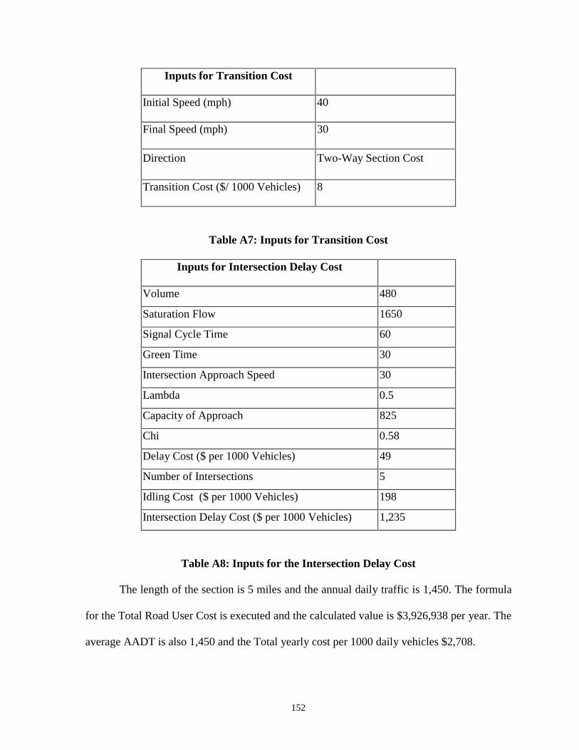
152
Inputs for Transition Cost
Initial Speed (mph) 40
Final Speed (mph) 30
Direction Two-Way Section Cost
Transition Cost ($/ 1000 Vehicles) 8
Table A7: Inputs for Transition Cost
Inputs for Intersection Delay Cost
Volume 480
Saturation Flow 1650
Signal Cycle Time 60
Green Time 30
Intersection Approach Speed 30
Lambda 0.5
Capacity of Approach 825
Chi 0.58
Delay Cost ($ per 1000 Vehicles) 49
Number of Intersections 5
Idling Cost ($ per 1000 Vehicles) 198
Intersection Delay Cost ($ per 1000 Vehicles) 1,235
Table A8: Inputs for the Intersection Delay Cost
The length of the section is 5 miles and the annual daily traffic is 1,450. The formula
for the Total Road User Cost is executed and the calculated value is $3,926,938 per year. The
average AADT is also 1,450 and the Total yearly cost per 1000 daily vehicles $2,708.