hot rolled wire descaling - chalmers publication...

Hot Rolled Wire Descaling

Master’s Thesis in Applied Physics

JON-HENRIK SVONNI

Department of Materials and Manufacturing TechnologyCHALMERS UNIVERSITY OF TECHNOLOGYGoteborg, Sweden 2012Master’s Thesis 2012:XX

MASTER’S THESIS

Hot Rolled Wire Descaling

Master’s Thesis in Applied PhysicsJON-HENRIK SVONNI

Department of Materials and Manufacturing TechnologyCHALMERS UNIVERSITY OF TECHNOLOGY

Goteborg, Sweden 2012

Hot Rolled Wire DescalingJON-HENRIK SVONNI

JON-HENRIK SVONNI, 2012

Master’s ThesisDepartment of Materials and Manufacturing Technology

Chalmers University of TechnologySE-412 96 GoteborgSwedenTelephone: + 46 (0)31-772 1000

Chalmers ReproserviceGoteborg, Sweden 2012

Hot Rolled Wire DescalingMaster’s Thesis in Applied PhysicsJON-HENRIK SVONNIDepartment of Materials and Manufacturing TechnologyChalmers University of Technology

Abstract

In the process of making welding wire an important step is to descale an oxide layerfrom the surface of the wire. If the oxide layer is not entirely removed it will affectthe quality of the finished product. A common way of descaling is to use acids whichis not quite environmental friendly. It is possible to mechanically descale the wirebut the method needs to be better since the current methods does not give consistentresults.

In this work the possiblity to descale the wire using ultrasounds have been inves-tigated. It has been theoretically analysed, modelled in MATLAB and comparedwith results from an existing mechanical wire descaler. The results have not beenvalidated through experimental analysis.

The results show that ultrasound may be an interesting technique to investigatefurther, and guidelines and important variables for future experiments are given.

, Materials and Manufacturing Technology, Master’s Thesis I

II , Materials and Manufacturing Technology, Master’s Thesis

Contents

Abstract I

Contents III

Preface V

Notation VI

1 Introduction 11.1 Background . . . . . . . . . . . . . . . . . . . . . . . . . . . . . . . . . . . 11.2 Purpose . . . . . . . . . . . . . . . . . . . . . . . . . . . . . . . . . . . . . 11.3 Limitations . . . . . . . . . . . . . . . . . . . . . . . . . . . . . . . . . . . 11.4 Aim . . . . . . . . . . . . . . . . . . . . . . . . . . . . . . . . . . . . . . . 11.5 Layout . . . . . . . . . . . . . . . . . . . . . . . . . . . . . . . . . . . . . . 1

2 Theory 22.1 Making Welding Wire . . . . . . . . . . . . . . . . . . . . . . . . . . . . . 2

2.1.1 Stelmor cooling . . . . . . . . . . . . . . . . . . . . . . . . . . . . . 32.1.2 Descaling . . . . . . . . . . . . . . . . . . . . . . . . . . . . . . . . 32.1.3 Coating and Drawing . . . . . . . . . . . . . . . . . . . . . . . . . . 3

2.2 Ultrasonic Cleaning . . . . . . . . . . . . . . . . . . . . . . . . . . . . . . . 42.3 Vibrating String . . . . . . . . . . . . . . . . . . . . . . . . . . . . . . . . . 52.4 Discretizing the Wave Equation . . . . . . . . . . . . . . . . . . . . . . . . 7

2.4.1 Matrix Representation . . . . . . . . . . . . . . . . . . . . . . . . . 82.5 Acoustic Pressure . . . . . . . . . . . . . . . . . . . . . . . . . . . . . . . . 82.6 The Wire Roll . . . . . . . . . . . . . . . . . . . . . . . . . . . . . . . . . . 102.7 The Bending Moment . . . . . . . . . . . . . . . . . . . . . . . . . . . . . . 102.8 Maximum Bending Momentum in the Elastic Region . . . . . . . . . . . . 11

3 Method 13

4 Results 154.1 Length and Tension Dependencies . . . . . . . . . . . . . . . . . . . . . . . 154.2 Model Eigenfrequencies . . . . . . . . . . . . . . . . . . . . . . . . . . . . . 184.3 Maximum Bend for Elastic Region . . . . . . . . . . . . . . . . . . . . . . 204.4 Wave Equation Simulations . . . . . . . . . . . . . . . . . . . . . . . . . . 21

4.4.1 The Frequency . . . . . . . . . . . . . . . . . . . . . . . . . . . . . 224.4.2 Constant F . . . . . . . . . . . . . . . . . . . . . . . . . . . . . . . 234.4.3 Constant p . . . . . . . . . . . . . . . . . . . . . . . . . . . . . . . 254.4.4 Constant l . . . . . . . . . . . . . . . . . . . . . . . . . . . . . . . . 274.4.5 Matrix Size . . . . . . . . . . . . . . . . . . . . . . . . . . . . . . . 28

5 Discussion 295.1 Length and Tension Dependencies . . . . . . . . . . . . . . . . . . . . . . . 295.2 Model Eigenfrequencies . . . . . . . . . . . . . . . . . . . . . . . . . . . . . 295.3 Maximum Bend for Elastic Region . . . . . . . . . . . . . . . . . . . . . . 295.4 Matrix Size . . . . . . . . . . . . . . . . . . . . . . . . . . . . . . . . . . . 29

, Materials and Manufacturing Technology, Master’s Thesis III

5.5 The Results from Constant F, p and l . . . . . . . . . . . . . . . . . . . . . 295.6 The Acoutic Pressure . . . . . . . . . . . . . . . . . . . . . . . . . . . . . . 30

6 Conclusion 316.1 Future Work . . . . . . . . . . . . . . . . . . . . . . . . . . . . . . . . . . . 31

IV , Materials and Manufacturing Technology, Master’s Thesis

Preface

This M.Sc. thesis has been conducted at ESAB Sweden and at Chalmers University ofTechnology at the department of Materials and Manufacturing Technology in the fall of2011.

Acknowledgements

I would like to thank: Lars Nyborg at Chalmers University of Technology that has beenthe examiner of this master’s thesis. Dean Ward and Jiri Hejcl at ESAB that have beenmy supervisors. I want to thank Peter Olsson, Lennart Josefsson and Hakan Wirdeliusand the NDT group at Chalmers University of Technology for ideas and help during theproject, and also Joel Kim at ESAB for support and feedback.

I also want to thank my family for all support throughout my time at Chalmers.

Goteborg March 2012Jon-Henrik Svonni

, Materials and Manufacturing Technology, Master’s Thesis V

Notations

M – Bending momentum [Nm]

T – Tension [N]

E – Young’s modulus [N/m2]

I – Second moment of area [m4]

ρ – Density [kg/m3]

A – Area [m2]

L – Length [m]

ω – Angular frequency [rad/s]

Pac – Acoustic power [W]

p – Sound pressure [Pa]

c – Sound velocity [m/s]

F – Force [N]

f – Frequency [Hz]

n – Eigenfrequency number

VI , Materials and Manufacturing Technology, Master’s Thesis

1 INTRODUCTION

1 Introduction

1.1 Background

Removing an oxide layer from the surface of welding wires is necessary in MAG (MetalActive Gas) production before the wire drawing process. The present method is not quiteenvironmental friendly because the usage of acids. When mechanically removing the scalessome sticky remain. These can also be removed by mechanical descaling but the resultsare not consistent but depend on the operator.

There are several different mechanical descalers today. An example is wire rolls: Thewelding wires are drawn over the rolls and the bending momentum makes the oxide scaleson the wire surface crack and fall off since they are less formable than the steel wire, butthe method is however not perfect. A suggested technique is to use ultrasonic vibrationsto achieve a similar bending momentums for better controllability and output.

1.2 Purpose

A need to investigate possible solutions for cleaner and quicker processes with better envi-ronmental control in the wire descaling process has been identified. The method needs tobe efficient and consistent.

1.3 Limitations

The work is limited to an analytical and computational analysis and does not includeexperimental validations. In the simulations the wire is assumed to be elastic. Ultrason-ics have been identified as a principle of interest and the work has been limited to onlyinvestigate this.

1.4 Aim

This project will start with an investigation of current options to define the direction ofnew technology and process in Hot rolled wire descaling. The process will be demonstratedwith MATLAB analysis to evaluate the theory and practice. The object of the project isto obtain a process modification for a cleaner, quicker and better environmental controlduring the process.

It has been suggested that by vibrating the wire at eigenfrequency to make it resonate couldproduce large enough vibrations to produce a bending momentum that pops off the oxidescales. The eigenfrequencies of a wire that is held in both ends have been been calculatedand the wire vibrations when subjected to a harmonic force at the eigenfrequency havebeen analysed through simulations.

1.5 Layout

The report is divided into six parts. After the introduction all theory needed for theunderstanding of the subsequent sections is given. In the others, the method is described,the results are presented, they are discussed and lastly conclusions from them are made.

, Materials and Manufacturing Technology, Master’s Thesis 1

2 THEORY

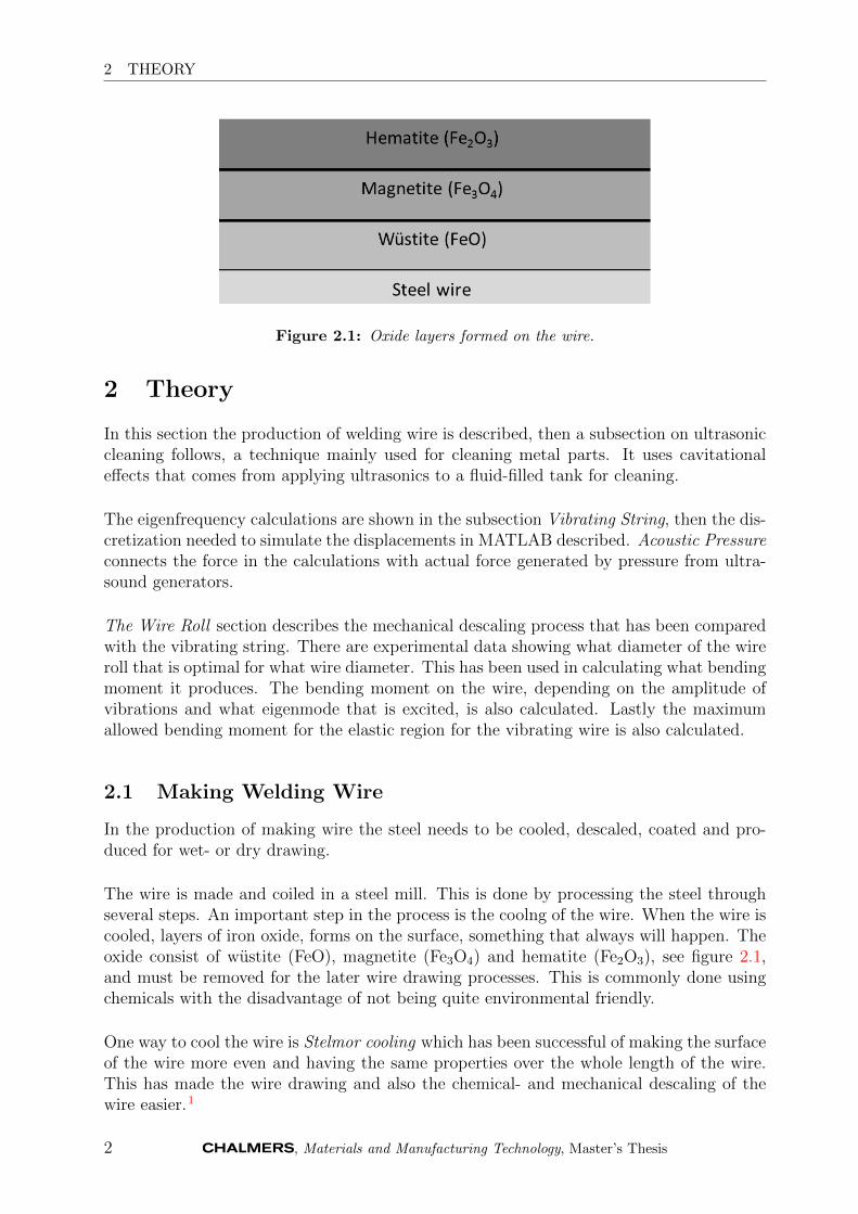
Figure 2.1: Oxide layers formed on the wire.

2 Theory

In this section the production of welding wire is described, then a subsection on ultrasoniccleaning follows, a technique mainly used for cleaning metal parts. It uses cavitationaleffects that comes from applying ultrasonics to a fluid-filled tank for cleaning.

The eigenfrequency calculations are shown in the subsection Vibrating String, then the dis-cretization needed to simulate the displacements in MATLAB described. Acoustic Pressureconnects the force in the calculations with actual force generated by pressure from ultra-sound generators.

The Wire Roll section describes the mechanical descaling process that has been comparedwith the vibrating string. There are experimental data showing what diameter of the wireroll that is optimal for what wire diameter. This has been used in calculating what bendingmoment it produces. The bending moment on the wire, depending on the amplitude ofvibrations and what eigenmode that is excited, is also calculated. Lastly the maximumallowed bending moment for the elastic region for the vibrating wire is also calculated.

2.1 Making Welding Wire

In the production of making wire the steel needs to be cooled, descaled, coated and pro-duced for wet- or dry drawing.

The wire is made and coiled in a steel mill. This is done by processing the steel throughseveral steps. An important step in the process is the coolng of the wire. When the wire iscooled, layers of iron oxide, forms on the surface, something that always will happen. Theoxide consist of wustite (FeO), magnetite (Fe3O4) and hematite (Fe2O3), see figure 2.1,and must be removed for the later wire drawing processes. This is commonly done usingchemicals with the disadvantage of not being quite environmental friendly.

One way to cool the wire is Stelmor cooling which has been successful of making the surfaceof the wire more even and having the same properties over the whole length of the wire.This has made the wire drawing and also the chemical- and mechanical descaling of thewire easier.1

2 , Materials and Manufacturing Technology, Master’s Thesis

2 THEORY

2.1.1 Stelmor cooling

In the Stelmor cooling process the wire initially gets cooled in water until the temperatureof the wire drops from 950 C◦, after this the wire is cooled in air to room temperature. Thelaying temperature i.e. the temperature in which the air cooling starts can be adjustedbetween about 875-750 C◦ and is very important for formation of different grain sizes andstructure. The cooling can also be slow or delayed with different handling of the wire.1

A study to investigate the formation of oxide depending on the cooling conditions of highcarbon wire rods have been conducted in laboratory simulations. During mechanical descal-ing the hematite layer is difficult to remove and tends to stick to the surface. This layerhas been shown to be significantly thinner with higher laying head temperature and fastercooling. At high temperatures, only wustit and magnetite are stable. Hematite formsas a decomposition of the high temperature oxides. If the cooling is fast less hematite isformed since there is less time for the oxides to decompose. Wustit and magnetite are lessadherent by nature and are therefore preferable. By keeping the laying head temperatureclose to 880 C◦ the hematite layer can be kept at a minimum. This was also reviewed andconfirmed in a test plant.2

2.1.2 Descaling

The oxide scales that are formed on the wire during the cooling needs to be removed inorder for the coating to stick in the next process step. This is usually done by acids or bymechanically removing them.

Chemical DescalingWhen chemically removing the scales with sulfuric acid (H2SO4) or hydrochloric acid (HCl)the acid penetrates the scales in cracks and attacks the wustite which is solvable in acids.The outer oxide layers are unaffected by the acid but gets undermined and therefore fallsoff. The environmental effects associated acids makes it interesting to evaluate mechanicaldescaling.1

Mechanical DescalingThere are several different ways of mechanically removing the scales. One method is calledscale breaking. The wire is bent over rolls so that the outer fibers is stretched so muchthat the scales break and fall off while the more formable steel remains. Scale breakingalways leaves some residues of the oxide and requires complementing methods to removethe rest. This can be done by brushing or by acids for instance. There are also severalother techniques to remove the scales mechanically, like for instance by shot blasting, jetbeam, shaving and with plasma.1

2.1.3 Coating and Drawing

After the descaling of the wire it gets coated and prepared for the drawing machine wherethe diameter of the wire is reduced to make welding wire.1


2 THEORY

2.2 Ultrasonic Cleaning

Ultrasonic cleaning has existed for decades and is used in several different industries. It canfor example remove oils, paints, dust and has also been successful of removing corrosiondeposits from metals. The benefits from ultrasonic cleaning can be lowered labor costs,less time comsumption and more reliable cleaning.3

The set up consists of ultrasonic transducers connected to diaphragms, a generator and atank filled with a cleaning liquid. The transducer is a piezo-ceramic material that changesits shape when it is excited by an electric signal. The piezo-electric transducer can beimmersed into the tank. When it gets excited by an high frequency electric generator itsvibrations get amplified by the diaphragm which causes compression and attenuation ofthe liquid in the tank. The liquid can be water or a cleaning chemical.3

The changes in density will start a cavitation process, bubbles will form and then im-plode. The frequency determines the magnitude of the bubbles. Low frequency produceslarger bubbles than high frequency. The cavitation effect is more aggressive with increasingbubble size. The energy release from bubble implosions close to the surface destroys thecontaminants, the implosion also creates a pressure wave and a high velocity jet and thecumulative effect of millions of implosions create the sufficient mechanical energy to breakthe contaminants bonds. The collapse of several cavities at the same time, clusters, maycause erosion of the sample.3

There are two mechanisms of ultrasonic cleaning, namely cavitation and acoustic stream-ing. When the cavitation bubbles implode they produce jets of liquid that can affect thesurface to be cleaned. The cavitation takes place at discontinuities of the surface suchas cracks and other features. The diameter of the bubbles are in the order of 100µm at25 kHz, and are generated on the order of microseconds with a estimated pressure of about50 MPa. Instantaneous collapse pressures from clusters in the order of 1 GPa have beenmeasured.3

In acoustic streaming the bulk liquid moves and the contaminants are carried away withit. Acoustic streaming is the dominating contribution of the cleaning at high frequencies,from about 170 kHz and even more over 1 MHz. At high frequencies the streaming veloc-ities are greater and the cavitation bubbles are smaller. The shear stress from acousticstreaming is non-erosive and strongly adhered particles cannot be removed from surfaces,it does however help to flush away loosened particles from the surface.3

Two frequencies can be used simultaneously to clean a surface with improved effect. Forexample can a high and a low frequency combination make the surface cleaner than thesum of cleaning with both frequencies individually.3


2 THEORY

2.3 Vibrating String

The mass of the wire is evenly distributed on the wire and the mass per unit length is ρ,the tension is T and when the wire is in rest it is on the x-axis. The wire is presumed toonly move in the xu-plane.

For a string with the tension T applied in both ends the equation of motion of the stringbecomes 2.1.4

∂2u

dt2= c2∂

2u

∂x2− β2∂

4u

∂x4(2.1)

β = (EIρA

)1/2, c = ( TρA

)1/2, A is the cross-section area, ρ is the density, E is Young’s modulus

and I is the second moment of area about the x-axis.4

The moment of inertia about the length axis is calculated as 2.2, or in cylindrical coordi-nates 2.3. The second area of moment is through the center of a homogenous wire withradius a constant in the x-direction and is I(x) = πa4

4.5

Iy(x) =

∫A

z2 dA (2.2)

I(x) =

∫ a

0

∫ 2π

0

r2sin2(φ) r drdφ (2.3)

The equation of motion is solved with the separtion method to determine the eigenfrequen-cies of the wire, 2.4.

u(x, t) = X(x)T (t) (2.4)

The separated equation of motion can now be solved. Since the X-equation and T-equationare independent of each other they must be equal to some constant λ, 2.5.

β2X(4)(x)

X(x)− c2X

′′(x)

X(x)= −T

′′(t)

T (t)= λ (2.5)

Because the solutions should be periodic λ must be positive. With λ = ω2 the solutionof the T-equation 2.6, is 2.7.

T ′′(t) = −ω2 T (t) (2.6)

T (t) = A1 sinωt+ A2 cosωt (2.7)

The X-equation 2.8 is solved by the ansatz X(x) = B es x and solving the characteristicequation 2.9. This gives the solutions s1 - s4, 2.10.

X(4)(x)− c2

β2X ′′(x)− ω2

β2X(x) = 0 (2.8)

s4 − c2

β2s2 − ω2

β2= 0 (2.9)


2 THEORY

s2 =c2

2β2±

√ω2

β2+

c4

4β4

⇒

s1 =

√c2

2β2 +√

ω2

β2 + c4

4β4

s2 = −√

c2

2β2 +√

ω2

β2 + c4

4β4

s3 = i

√√ω2

β2 + c4

4β4 − c2

2β2

s4 = −i√√

ω2

β2 + c4

4β4 − c2

2β2

(2.10)

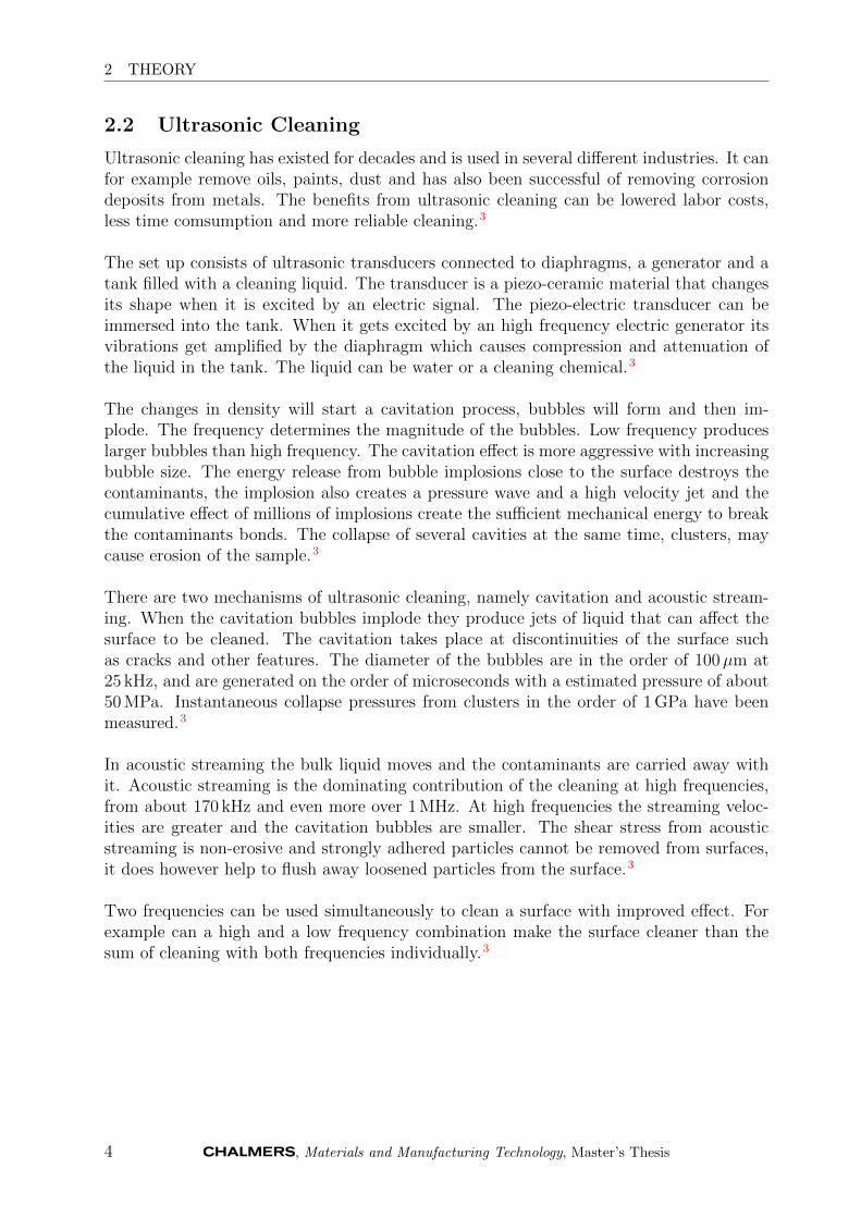
s1 = −s2 and s3 = −s4. Since s3 is imaginary, s3 will be the imaginary part from here oni.e. the root is is3. The solution can be written as 2.11, this is modified to 2.13 throughthe relations 2.12.

X(x) = B1 es1 x +B2 e

−s1 x +B3 eis3 x +B4 e

−is3 x (2.11)

sinh s1 x =es1 x − e−s1 x

2

cosh s1 x =es1 x + e−s1 x

2

sin s3 x =eis3 x − e−is3 x

2i

cos s3 x =eis3 x + e−is3 x

2

(2.12)

X(x) = B′1 sinh s1 x+B′2 cosh s1 x+B′3 sin s3 x+B′4 cos s3 x (2.13)

The boundary conditions that the lateral movement and the moment in the ends are zero(X(0) = 0 and X ′′(0) = 0) gives that B′2 and B′4 has to be zero, 2.14.{

X(0) = B′2 +B′4 = 0

X ′′(0) = s22B′2 − s2

4B′4 = 0

(2.14)

The equation is now simplified to 2.15.

X(x) = B′1 sinh s1 x+B′3 sin s3 x (2.15)

The conditions X(L) = 0 and X ′′(L) = 0 gives the equation system 2.16. Combing thesegives 2.17. Multiplying the equations in 2.16 gives 2.18 and inserting 2.17 gives the relationneeded for finding the eigenfrequencies.{

B′1 sinh s1 L+B′3 sin s3 L = 0

s21B′1 sinh s1 L− s2

3B′3 sin s3 L = 0

(2.16)

B′1 = −B′3sin s3 L

sinh s1 L(2.17)


2 THEORY

s21B′21 sinh2 s1 L− s2

3B′23 sin2 s3 L︸︷︷︸

=(s21−s23)B′23 sin2 s3 L

+ (s21 − s2

3)︸︷︷︸=( c

β)2

B′1B′3 sinh s1 L sin s3 L = 0 (2.18)

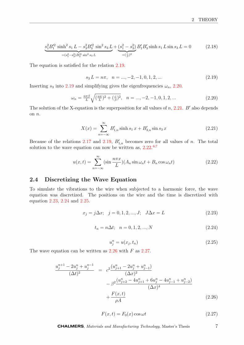
The equation is satisfied for the relation 2.19.

s3 L = nπ, n = ...,−2,−1, 0, 1, 2, ... (2.19)

Inserting s3 into 2.19 and simplifying gives the eigenfrequencies ωn, 2.20.

ωn = nπβL

√(nπL

)2 + ( cβ)2, n = ...,−2,−1, 0, 1, 2, ... (2.20)

The solution of the X-equation is the superposition for all values of n, 2.21. B′ also dependson n.

X(x) =∞∑

n=−∞

B′1,n sinh s1 x+B′3,n sin s3 x (2.21)

Because of the relations 2.17 and 2.19, B′1,n becomes zero for all values of n. The totalsolution to the wave equation can now be written as, 2.22.6;7

u(x, t) =∞∑

n=−∞

(sinnπx

L)(An sinωnt+Bn cosωnt) (2.22)

2.4 Discretizing the Wave Equation

To simulate the vibrations to the wire when subjected to a harmonic force, the waveequation was discretized. The positions on the wire and the time is discretized withequation 2.23, 2.24 and 2.25.

xj = j∆x; j = 0, 1, 2, ..., J ; J∆x = L (2.23)

tn = n∆t; n = 0, 1, 2, ..., N (2.24)

unj = u(xj, tn) (2.25)

The wave equation can be written as 2.26 with F as 2.27.

un+1j − 2unj + un−1

j

(∆t)2= c2

(unj+1 − 2unj + unj−1)

(∆x)2

− β2(unj+2 − 4unj+1 + 6unj − 4unj−1 + unj−2)

(∆x)4

+F (x, t)

ρA(2.26)

F (x, t) = F0(x) cosωt (2.27)


2 THEORY

This gives the relation for the next time-step, 2.28.

un+1j = (2− 2r2 − 6r2s2)unj − un−1

j

+ (r2 + 4r2s2)[unj+1 + unj−1]

− r2s2[unj+2 + unj−2]

+F (x, t)(∆t)2

ρA(2.28)

r = c∆t∆x

and s = β∆x

.

2.4.1 Matrix Representation

The discretization was represented in a J × J matrix, 2.29. With the next time step as2.30. The values of α− ε are correspondin to equation 2.28 with α = ε, β = δ. α = − r2s2,β = (r2 + 4r2s2), γ = (2− 2r2− 6r2s2) and B is a diagonal matrix with the value -1 on allnon-zero elements.

A =

γ δ ε 0 0 0 . . .β γ δ ε 0 0 . . .α β γ δ ε 0 . . .0 α β γ δ ε . . .

. . . . . . . . . . . . . . . . . . . . .

. . . 0 0 α β γ δ

. . . 0 0 0 α β γ

(2.29)

un+1j = Aunj + Bun−1

j +F0(x)(∆t)2 cosωt

ρA(2.30)

The eigenfrequencies of the model with the matrix size J × J is determined by taking thesquare root of the eigenvalues calculated by using the MATLAB command eig on A, andthen plotted for increasing n to compare with the analytical eigenfrequencies.

2.5 Acoustic Pressure

A point source for acoustic pressure is used to determine what power the generator needsto have to achieve the needed force on the wire.

The sound power Pac, for plane sound waves are given by equation 2.31. p is the soundpressure, As is the area of a sphere with the radius r from the point source, cf is thevelocity of sound in the medium and ρf is the density of given medium.

Pac =p2Ascfρf

(2.31)

As = 4πr2, this gives the equation for the sound pressure as 2.32. The sound pressuredecreases with the distance with 1/r.

p =1

r

√Pac cf ρf

4π(2.32)


2 THEORY

The total force F added to the right hand side of the discretized wave equation 2.26 is thesum of the F0 elements, 2.33. m is the number of elements that F is applied to.

Ftot = mF0 (2.33)

The total force is also the acoustic pressure times the area which is the length x multipliedby the diameter of the wire that the pressure is applied to, 2.34.

Ftot = pxd (2.34)

Equation 2.33 and 2.34 gives the relation between the force used in the discretized waveequation and the pressure, see equation 2.35.

p =mF0

xd(2.35)

With the relations 2.35 and 2.32 it is possible to determine what power the generator needsto have and what distance it needs to have to the wire for a specified medium.


2 THEORY

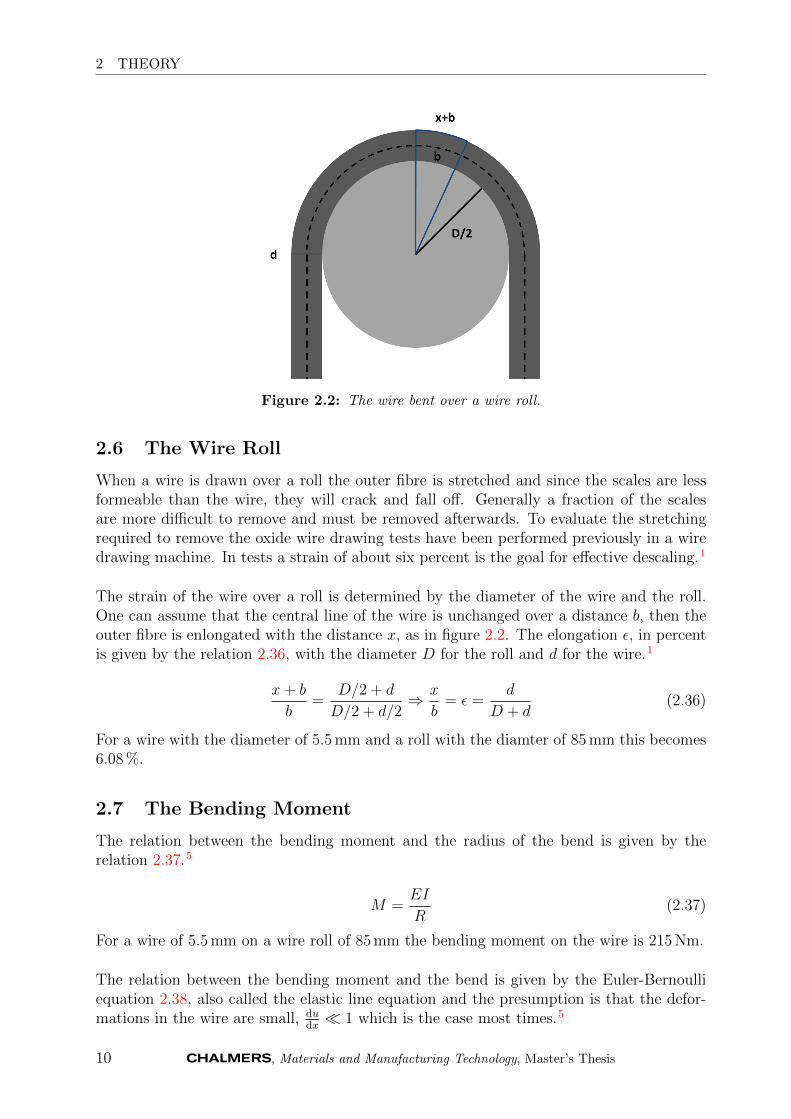
Figure 2.2: The wire bent over a wire roll.

2.6 The Wire Roll

When a wire is drawn over a roll the outer fibre is stretched and since the scales are lessformeable than the wire, they will crack and fall off. Generally a fraction of the scalesare more difficult to remove and must be removed afterwards. To evaluate the stretchingrequired to remove the oxide wire drawing tests have been performed previously in a wiredrawing machine. In tests a strain of about six percent is the goal for effective descaling.1

The strain of the wire over a roll is determined by the diameter of the wire and the roll.One can assume that the central line of the wire is unchanged over a distance b, then theouter fibre is enlongated with the distance x, as in figure 2.2. The elongation ε, in percentis given by the relation 2.36, with the diameter D for the roll and d for the wire.1

x+ b

b=

D/2 + d

D/2 + d/2⇒ x

b= ε =

d

D + d(2.36)

For a wire with the diameter of 5.5 mm and a roll with the diamter of 85 mm this becomes6.08 %.

2.7 The Bending Moment

The relation between the bending moment and the radius of the bend is given by therelation 2.37.5

M =EI

R(2.37)

For a wire of 5.5 mm on a wire roll of 85 mm the bending moment on the wire is 215 Nm.

The relation between the bending moment and the bend is given by the Euler-Bernoulliequation 2.38, also called the elastic line equation and the presumption is that the defor-mations in the wire are small, du

dx� 1 which is the case most times.5


2 THEORY

M = −EI d2u

dx2(2.38)

The displacement of the wire is calculated before, in equation 2.22. It is therefore possibleto derive it twice and calculate the bending moment at the point where the displacementis the largest, at Cmax, 2.39.

Mmax = EI (nπ

L)2Cmax (2.39)

2.8 Maximum Bending Momentum in the Elastic Region

To determine how much the wire may be displaced and still be in the elastic region can bedone by integrating the curve and plotting the result in MATLAB. The possible displace-ment is dependent on what wave mode is excited i.e. what n is used.

To do this the length of the wire in rest is compared with the wire when it has the amplitudeC. Then it can be calculated for different frequencies. The wire has a sinusoidal curvature,2.40. To evaluate it, x and y has to be expressed in the same variable, 2.41.

y(x) = C sinnπx

L(2.40)

r(θ) = (x(θ), y(θ)) (2.41)

This is done with elliptical coordinates as in equation 2.42.{y(θ) = L

2nsin θ

x(θ) = C cos θ(2.42)

The length of a curve s is calculated with equation 2.43.8

s =

∫Γ

ds =

∫ b

a

|r(θ)| dθ (2.43)

Inserting 2.42 gives equation 2.44.

s =

∫ π/2

0

√x(θ)2 + y(θ)2 dθ (2.44)

After some simplifications this results in an elliptical integral 2.45, that needs to be solvedwith tabular values.8

s = L2n

∫ π/20

√√√√√1− (1− (C

L/2n))2︸︷︷︸

k2

sin2 θ dθ , (k2 < 1)(2.45)

The value L2n

in front of the integral is the length of the wire in rest. So the value ofthe integral is therefore the elongation factor ε. The tabular values for different values ofε is listed with correspoding values for k is listed in 2.47. The k value for the differentelongations is given by 2.46.


2 THEORY

k = sinα (2.46)

ε = 1.01 ⇒ α = 85.6◦

ε = 1.02 ⇒ α = 83.6◦

ε = 1.03 ⇒ α = 81.6◦ (2.47)

The amplitude C is used when calculating the bending moment. By combining k fromequation 2.45 and 2.46 an equation for the maximum displacement for different elongationscan be calculated, 2.48. This is used for calculating the maximum bend with equation 2.39.

C =L

2n

√1− sin2 α (2.48)


3 METHOD

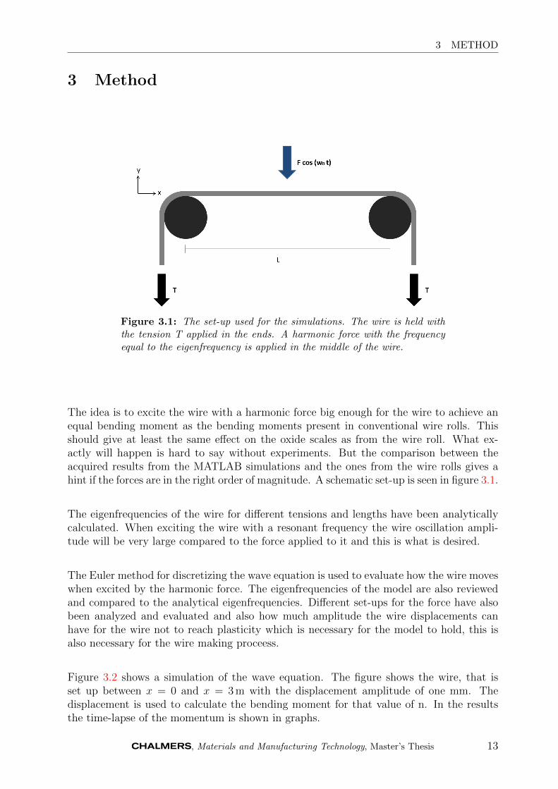
3 Method

Figure 3.1: The set-up used for the simulations. The wire is held withthe tension T applied in the ends. A harmonic force with the frequencyequal to the eigenfrequency is applied in the middle of the wire.

The idea is to excite the wire with a harmonic force big enough for the wire to achieve anequal bending moment as the bending moments present in conventional wire rolls. Thisshould give at least the same effect on the oxide scales as from the wire roll. What ex-actly will happen is hard to say without experiments. But the comparison between theacquired results from the MATLAB simulations and the ones from the wire rolls gives ahint if the forces are in the right order of magnitude. A schematic set-up is seen in figure 3.1.

The eigenfrequencies of the wire for different tensions and lengths have been analyticallycalculated. When exciting the wire with a resonant frequency the wire oscillation ampli-tude will be very large compared to the force applied to it and this is what is desired.

The Euler method for discretizing the wave equation is used to evaluate how the wire moveswhen excited by the harmonic force. The eigenfrequencies of the model are also reviewedand compared to the analytical eigenfrequencies. Different set-ups for the force have alsobeen analyzed and evaluated and also how much amplitude the wire displacements canhave for the wire not to reach plasticity which is necessary for the model to hold, this isalso necessary for the wire making proceess.

Figure 3.2 shows a simulation of the wave equation. The figure shows the wire, that isset up between x = 0 and x = 3 m with the displacement amplitude of one mm. Thedisplacement is used to calculate the bending moment for that value of n. In the resultsthe time-lapse of the momentum is shown in graphs.


3 METHOD

Figure 3.2: The set-up for the bending moment simulations. Here awire that is excited with n=21.


4 RESULTS

4 Results

This section contains the results of the simulations in MATLAB. In the simulations valuesfor a steel wire with the diameter 5.5 mm has been used.

4.1 Length and Tension Dependencies

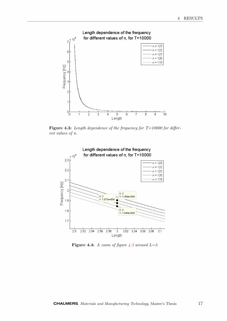
The results from the simulations to determine the length dependence of the tension andfrequency, is shown in figure 4.1 and 4.2 and figure 4.3 and 4.4 respectively. n = 121 isequal to f = 18735 Hz.

Figure 4.1 and the zoomed in figure 4.2 shows that in order to steer the eigenfrequenciesa length of at least 3 m is needed. The eigenfrequencies are very close to each other fordifferent tensions. For subsequent simulations a tension of 10 kN has been used.

Figure 4.3 and the zoomed in 4.4 shows how close in frequency the different eigenmodesare.


4 RESULTS

Figure 4.1: Length dependence of the frequency for n=121 for differentvalues of the tension.

Figure 4.2: A zoom of figure 4.1 around L=3.


4 RESULTS

Figure 4.3: Length dependence of the frequency for T=10000 for differ-ent values of n.

Figure 4.4: A zoom of figure 4.3 around L=3.


4 RESULTS

4.2 Model Eigenfrequencies

The model eigenfrequencies has been compared with the analytical eigenvalues. For thelow eigenmodes the model is quite accurate but for big values of n the values diverges. Theshift of the model eigenfrequencies for a thousand elements (J=1000) is seen in figure 4.5and 4.6.

Figure 4.5: The eigenfrequencies for different values of n.


4 RESULTS

Figure 4.6: A zoom of figure 4.5 around n=121.


4 RESULTS

4.3 Maximum Bend for Elastic Region

In figure 4.7 the maximum possible bend for different elongations is shown.

Higher frequencies makes it possible to achieve larger bending moments by less stretchingof the wire. The wire can reach a bending moment of 215 Nm at the frequency of 0.25 MHzwithout stretching the wire more than 0.2%.

Figure 4.7: The maximum possible bend for different frequencies, for thewire without elongating it more than ε. The bending moment for n=121is 215.8 Nm.


4 RESULTS

4.4 Wave Equation Simulations

The simulations for the wave equation contains a time-lapse over the calculated bendingmoment. The interesting part is the maximum value of the curve. The bending momentgoes up and down with the frequency of the harmonic force because of the flattening ofthe wire between the maxima. When the wire oscillates close to the eigenfrequency, theamplitude of the oscillations increase.

The following section is divided into subsections where different aspects of the applied forceand the model is looked in to. These are:- The Frequency- Constant F- Constant p- Constant l- and the Matrix Size


4 RESULTS

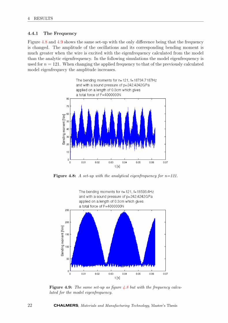
4.4.1 The Frequency

Figure 4.8 and 4.9 shows the same set-up with the only difference being that the frequencyis changed. The amplitude of the oscillations and its corresponding bending moment ismuch greater when the wire is excited with the eigenfrequency calculated from the modelthan the analytic eigenfrequency. In the following simulations the model eigenfrequency isused for n = 121. When changing the applied frequency to that of the previously calculatedmodel eigenfrequecy the amplitude increases.

Figure 4.8: A set-up with the analytical eigenfrequency for n=121.

Figure 4.9: The same set-up as figure 4.8 but with the frequency calcu-lated for the model eigenfrequency.


4 RESULTS

4.4.2 Constant F

A set-up with constant total force and increasing area that the force is distributed on isshown in figure 4.10, 4.11 and 4.12. When the force is distributed over a larger area theamplitude of the bending moment decreases, but less pressure is needed. When the areafurther inreases the efficiency drops even more.

Figure 4.10: Set-up A for constant F.

Figure 4.11: Set-up B for constant F.


4 RESULTS

Figure 4.12: Set-up C for constant F.


4 RESULTS

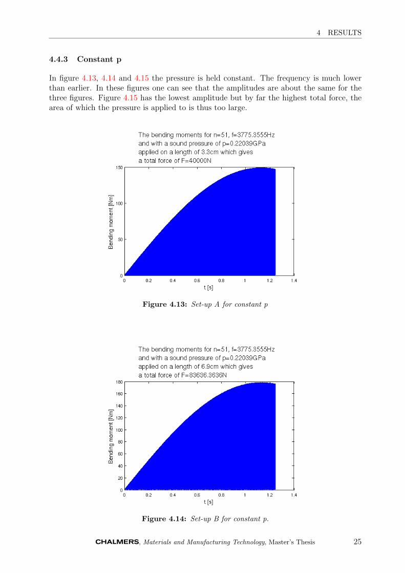
4.4.3 Constant p

In figure 4.13, 4.14 and 4.15 the pressure is held constant. The frequency is much lowerthan earlier. In these figures one can see that the amplitudes are about the same for thethree figures. Figure 4.15 has the lowest amplitude but by far the highest total force, thearea of which the pressure is applied to is thus too large.

Figure 4.13: Set-up A for constant p

Figure 4.14: Set-up B for constant p.


4 RESULTS

Figure 4.15: Set-up C for constant p.


4 RESULTS

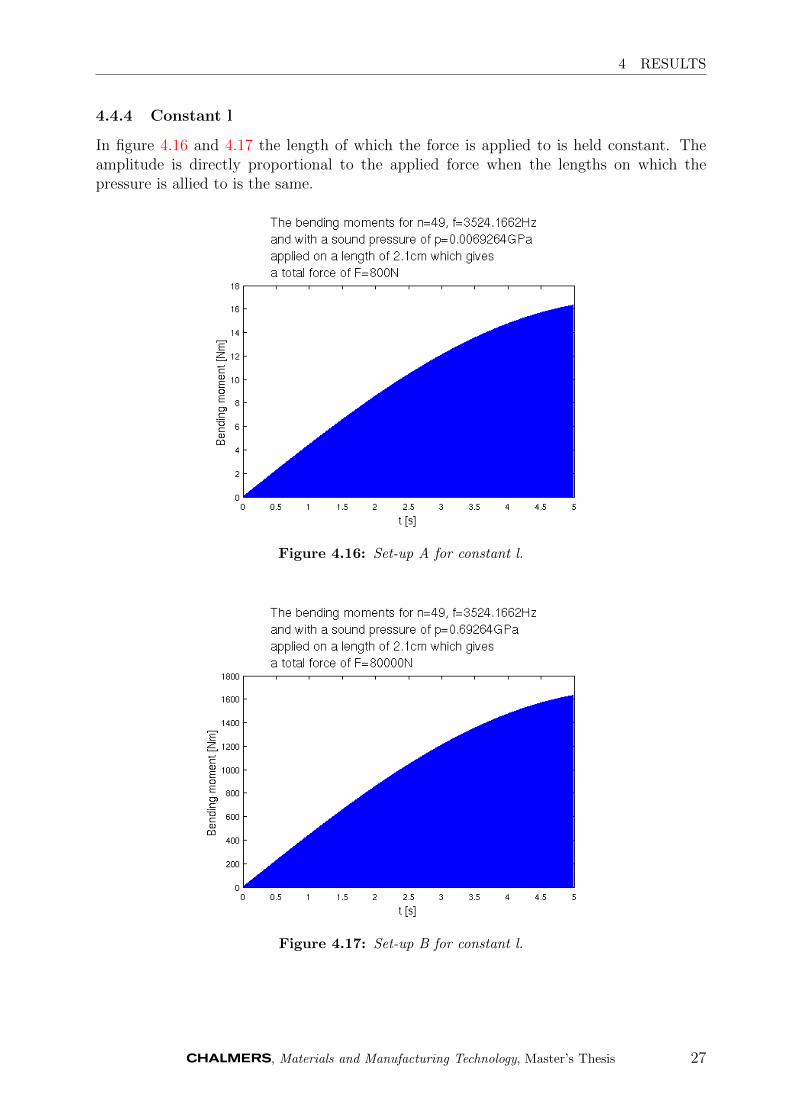
4.4.4 Constant l

In figure 4.16 and 4.17 the length of which the force is applied to is held constant. Theamplitude is directly proportional to the applied force when the lengths on which thepressure is allied to is the same.

Figure 4.16: Set-up A for constant l.

Figure 4.17: Set-up B for constant l.


4 RESULTS

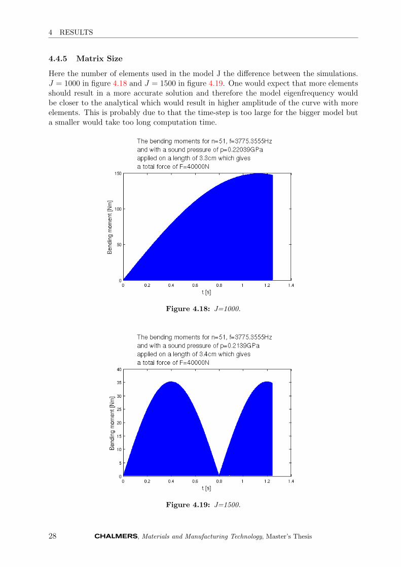
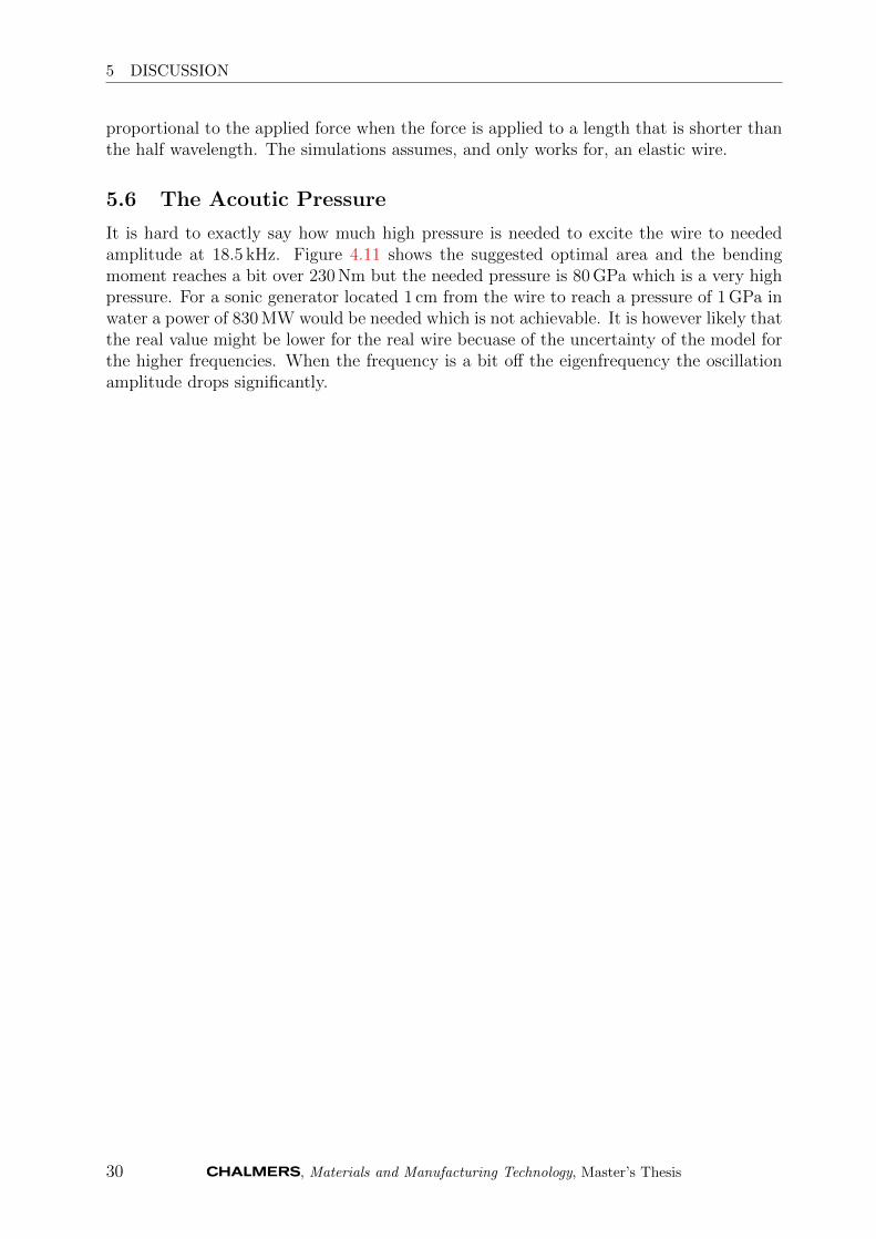
4.4.5 Matrix Size

Here the number of elements used in the model J the difference between the simulations.J = 1000 in figure 4.18 and J = 1500 in figure 4.19. One would expect that more elementsshould result in a more accurate solution and therefore the model eigenfrequency wouldbe closer to the analytical which would result in higher amplitude of the curve with moreelements. This is probably due to that the time-step is too large for the bigger model buta smaller would take too long computation time.

Figure 4.18: J=1000.

Figure 4.19: J=1500.


5 DISCUSSION

5 Discussion

Here follows a discussion of the results.

5.1 Length and Tension Dependencies

The length dependence of the eigenfrequencies shows that a set-up where the wire lengthis at least 3 m is desired because shorter lengths make the controllability of the eigenfre-quencies much more difficult. Also, with too long wire other effects might take place suchas the wire collapsing of its own weight. The tension can be selected freely with the onlyconstraint that it must hold the wire still.

5.2 Model Eigenfrequencies

The model eigenfrequencies results show that the model is quite good for predicting theeigenfrequency, although there is a small shift in frequency especially for higher frequen-cies. It is possible that this affects the results for n = 121 in a way that the model mightbe insufficient for determining the correct force needed to achieve the desired amplitude.

5.3 Maximum Bend for Elastic Region

These calculation says that the frequency must be at least 18.5 kHz (n = 121) to achievesufficiently large oscillations for the bending momentum to reach 215 Nm without elon-gating the wire more than 2%. Higher than 2% elongation can not be accepted due toplasticity. Lower frequencies can not achieve that bending moment without stretching thewire over the plasticity limit. The wire might reach plasticity already on 0.2% elongationin the radial direction, that would require the frequency to be 0.25 MHz.

5.4 Matrix Size

For the simulations, there are always one thousand elements that are evaluated, exceptin the section about the matrix size. The results from this section indicates that even ifmore positions on the wire is evaluated the result is not better. This is probably due tothat the time-steps are to big and thus the bending moment becomes less than for thesimulation with J = 1000 even though the result should be more accurate with more cells.By decreasing the time-step size the simulation time quickly becomes too long.

5.5 The Results from Constant F, p and l

From these simulations one can see that the amplitude of the wire depends on what totalforce is applied. If the force is spread out over a length that is longer than ≈ 1

2wavelength

the effect is lowered. For n = 121 that is L2n

= 1.2 cm and for n = 51 this value is2.9 cm. From the constant l simulations one can see that the bending moment is directly


5 DISCUSSION

proportional to the applied force when the force is applied to a length that is shorter thanthe half wavelength. The simulations assumes, and only works for, an elastic wire.

5.6 The Acoutic Pressure

It is hard to exactly say how much high pressure is needed to excite the wire to neededamplitude at 18.5 kHz. Figure 4.11 shows the suggested optimal area and the bendingmoment reaches a bit over 230 Nm but the needed pressure is 80 GPa which is a very highpressure. For a sonic generator located 1 cm from the wire to reach a pressure of 1 GPa inwater a power of 830 MW would be needed which is not achievable. It is however likely thatthe real value might be lower for the real wire becuase of the uncertainty of the model forthe higher frequencies. When the frequency is a bit off the eigenfrequency the oscillationamplitude drops significantly.


6 CONCLUSION

6 Conclusion

For ultrasound cleaning to work properly the surface needs to have discontinuities for thecavitation erosion to be effective. This leads to the idea of adding an ultrasound generatoracting on a small area whos function is to make the wire vibrate to loosen the scales.To add the extra ultrasound generator into the tank used for ultrasound cleaning makesadditional preparations for the wire unneccessary. Using dual frequencies for eroding theoxide and cleaning the wire as suggested by Kohli and Mittal may erase the need for afterwork. The Stelmor cooling process should also be optimized for minimizing the hematitelayer. It is uncertain exactly how much power the ultrasound generator needs to emit tosuccessfully vibrate the wire with sufficient amplitude. The effects from cavitation knownfrom the concept of ultrasound cleaning may add additional pressure, the effect from thisis not included in this work.

6.1 Future Work

A future work to evaluate the concept in practice would be a very interesting task andneeded to be able to validate the results and also to be able to see how much pressure thatis possible to attain at the surface of the wire.


REFERENCES

References

[1] Per Enghag. Tradteknik. Materialteknik, Orebro, Sweden, 2010.

[2] A. Chattopadhyay et al. Study on formation of ”easy to remove oxide scale” dur-ing mechanical descaling of high carbon wire rods. Surface & Coatings Technology,203:2912–2915, 2009.

[3] Rajiv Kohli and Kashmiri L. Mittal. Developments in Surface Contamination andCleaning – Particle Deposition, Control and Removal. Elsevier Inc., Amsterdam,Netherlands, 2009.

[4] Peter Olsson. Svangningar och Ljudutbredning, Del 1: Endimensionella System. Avdel-ning Mekanik CTH, Goteborg, Sweden, 1989.

[5] Hans Lundh. Grundlaggande hallfasthetslara. Kungliga tekniska hogskolan. Institutio-nen for hallfasthetslara, Stockholm, Sweden, 2007.

[6] Gerald B. Folland. Fourier analysis and its applications. Wadsworth & Brooks/Cole,Pacific Grove, California, 1992.

[7] Singiresu S. Rao. Mechanical Vibrations, 4th edition. Pearson Education, Inc, UpperSaddle River, New Jersey, 2004.

[8] Lennart Rade and Bertil Westergren. Mathematics Handbook. Studentlitteratur, Lund,Sweden, 2008.


hot rolled wire descaling - chalmers publication...

Documents