household travel model - squarespace · household travel app 3 introduction some of today’s most...

HOUSEHOLD TRAVEL APP

Reid Ewing

University of Utah

11/30/12

Household Travel App

1

Contents

Executive Summary ......................................................................................................................... 2

D Variables ...................................................................................................................................... 3

Literature ........................................................................................................................................ 4

Self-Selection .................................................................................................................................. 7

Methods .......................................................................................................................................... 8

Data ................................................................................................................................................. 8

Variables........................................................................................................................................ 10

Statistical Analysis ......................................................................................................................... 11

Results ........................................................................................................................................... 14

Discussion...................................................................................................................................... 18

References .................................................................................................................................... 18


2

Executive Summary

The potential to moderate travel demand by changing the built environment is the most heavily

researched subject in urban planning. Yet, the existing literature is short on external validity or

generalizability. The models estimated for Portland, OR or Southern California cannot necessarily be

applied to the rest of the United States. To fill this gap in the literature, we have estimated travel models

based on pooled household travel data and built environment data from six diverse regions of the United

States. This application, referred to as the Household Travel App, is perhaps the most critical of all

within the scenario planning software package, Envision Tomorrow Plus (ET+). The reason is that the

outputs of this app feed into many other apps.

The Household Travel App consists of five models, with household travel outcomes as the dependent

variables, and so-called D variables as the independent variables. The predicted outcomes are vehicle

trips, walk trips, bike trips, transit trips, and vehicle miles traveled (VMT). The D variables are the

demographics of households and the density, diversity, design, destination accessibility, and distance to

transit for buffers around their places of residence. The six D’s affect the accessibility of trip productions

to trip attractions, and hence the generalized cost of travel by different modes to and from different

locations. This affects the utility of different travel choices.

Multilevel modeling (MLM) is used to account for dependence among observations, in this case the

dependence of households within a given region. All households within a given region share the

characteristic of that region. This dependence violates the independences assumption of ordinary least

squares (“OLS”) regression. Therefore, MLM produces a more accurate coefficient and standard error

estimates.

VMT increases with the household size, number of employed household members, and real household

income. The coefficient values suggest that household VMT does not rise as fast household size or

income. Household VMT declines with four built environmental variables characterizing one-mile

buffers around households: activity density, intersection density, percentage of 4-way intersections, and

transit stop density. In addition, VMT declines as the percentage of regional employment accessible

within a 10 minute drive time increases. Again, those who live in highly accessible places (characterized

by these five D variables) generate less VMT than those in less accessible places.

The number of household walk trips increases with household size and declines with household income.

High income households have greater access to private vehicles. Walk trips increase with land use

entropy (mix) within a quarter mile of home and activity density within a mile of home. These measures

of density and diversity place destinations within walking distance of home. Walk trips also increase with

transit stop density within a mile of home. Transit service is complementary to walking, as households

with good access to transit own fewer private vehicles and hence are more likely to use alternative modes.

The bike trip model is the simplest of the six models estimated. Bike trip frequency increases with

household size, land use entropy within a quarter mile, activity density within a mile, and percentage of 4-

way intersections within a mile. All three built environmental variables tend to reduce bicycling

distances between home and trip attractions, thereby reducing the generalized cost of bicycling relative to

automobile use.

The number of household transit trips increases with household size and employment, and declines with

household income. The number increases with land use entropy, activity density, and percentage of 4-

way intersections. Transit-oriented development is virtually defined by these three variables. Controlling

for these variables, transit trips increase with two transit service variables, transit stop density within a

quarter mile and percentage of regional employment reachable within 30 minutes by transit.


3

Introduction

Some of today’s most vexing problems, including sprawl, congestion, oil dependence, and climate

change, are prompting states and localities to turn to land planning and urban design to rein in automobile

use. But how much effect can land planning and urban design have on automobile use, walking, biking,

and transit use?

This chapter describes the 6D household travel app. This application within the Envision Tomorrow Plus

(ET+) suite is perhaps the most critical of all. This is because the outputs of this app feed into many other

apps. For example, the vehicle emission app depends on two outputs of this app, household vehicle miles

traveled (VMT) and household vehicle trips (VT). The public health app depends on three outputs, walk

bike, and transit trip frequency. All told, six apps are linked to this one app.

D Variables

The potential to moderate travel demand by changing the built environment is the most heavily

researched subject in urban planning. In travel research, such influences have often been named with

words beginning with D. The original “three Ds,” coined by Cervero and Kockelman (1997), are density,

diversity, and design, followed later by destination accessibility and distance to transit (Ewing & Cervero,

2001; Ewing and Cervero, 2010; Ewing, Greenwald, & Zhang, 2011). While not part of the environment,

demographics are the sixth D, controlled as confounding influences in travel studies.

A number of studies, including Crane (1996), Cervero and Kockelman (1997), Kockelman (1997),

Boarnet and Crane (2001), Cervero (2002a), Zhang (2004), and Cao, Mokhtarian, and Handy (2009b),

provide economic and behavioral explanations of why built environments might be expected to influence

travel choices. Basically, the first six Ds affect the accessibility of trip productions to trip attractions, and

hence the generalized cost of travel by different modes to and from different locations. This, in turn,

affects the utility of different travel choices. For example, destinations that are closer as a result of

higher density or greater diversity are easier to walk to than distant destinations. As the Ds increase (and

distance to transit decreases), the generalized cost of travel by alternative modes decreases, relative utility

increases, and mode shifts occur.

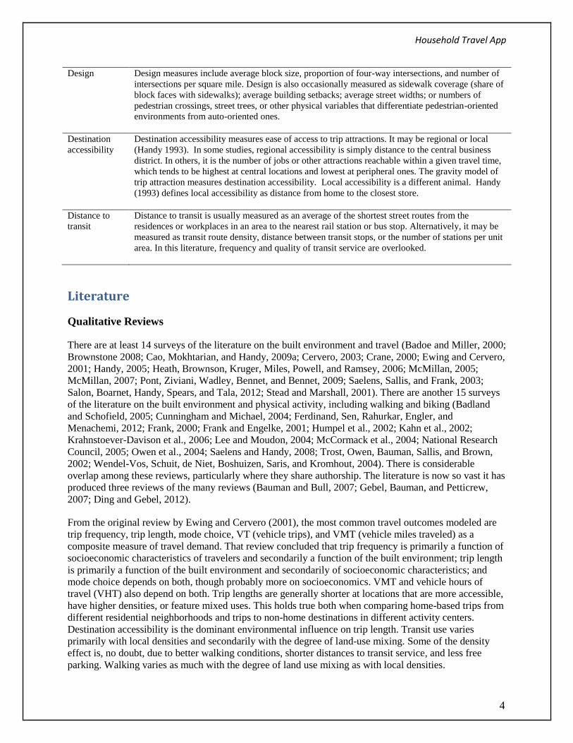
Table 1 indicates how D variables are typically measured. Note that these are rough categories, divided

by ambiguous and unsettled boundaries that may change in the future. Some dimensions overlap (e.g.,

diversity and destination accessibility). Still, it is a useful framework to organize the empirical literature

and provide order-of-magnitude insights.

Table 1. The D Variables

D Variable Measurement

Density Density is always measured as the variable of interest per unit of area. The area can be gross or

net, and the variable of interest can be population, dwelling units, employment, or building floor

area. Population and employment are sometimes summed to compute an overall activity density

per areal unit.

Diversity Diversity measures pertain to the number of different land uses in a given area and the degree to

which they are represented in land area, floor area, or employment. Entropy measures of diversity,

wherein low values indicate single-use environments and higher values more varied land uses, are

widely used in travel studies. Jobs-to-housing or jobs-to-population ratios are less frequently used.


4

Design Design measures include average block size, proportion of four-way intersections, and number of

intersections per square mile. Design is also occasionally measured as sidewalk coverage (share of

block faces with sidewalks); average building setbacks; average street widths; or numbers of

pedestrian crossings, street trees, or other physical variables that differentiate pedestrian-oriented

environments from auto-oriented ones.

Destination

accessibility

Destination accessibility measures ease of access to trip attractions. It may be regional or local

(Handy 1993). In some studies, regional accessibility is simply distance to the central business

district. In others, it is the number of jobs or other attractions reachable within a given travel time,

which tends to be highest at central locations and lowest at peripheral ones. The gravity model of

trip attraction measures destination accessibility. Local accessibility is a different animal. Handy

(1993) defines local accessibility as distance from home to the closest store.

Distance to

transit

Distance to transit is usually measured as an average of the shortest street routes from the

residences or workplaces in an area to the nearest rail station or bus stop. Alternatively, it may be

measured as transit route density, distance between transit stops, or the number of stations per unit

area. In this literature, frequency and quality of transit service are overlooked.

Literature

Qualitative Reviews

There are at least 14 surveys of the literature on the built environment and travel (Badoe and Miller, 2000;

Brownstone 2008; Cao, Mokhtarian, and Handy, 2009a; Cervero, 2003; Crane, 2000; Ewing and Cervero,

2001; Handy, 2005; Heath, Brownson, Kruger, Miles, Powell, and Ramsey, 2006; McMillan, 2005;

McMillan, 2007; Pont, Ziviani, Wadley, Bennet, and Bennet, 2009; Saelens, Sallis, and Frank, 2003;

Salon, Boarnet, Handy, Spears, and Tala, 2012; Stead and Marshall, 2001). There are another 15 surveys

of the literature on the built environment and physical activity, including walking and biking (Badland

and Schofield, 2005; Cunningham and Michael, 2004; Ferdinand, Sen, Rahurkar, Engler, and

Menachemi, 2012; Frank, 2000; Frank and Engelke, 2001; Humpel et al., 2002; Kahn et al., 2002;

Krahnstoever-Davison et al., 2006; Lee and Moudon, 2004; McCormack et al., 2004; National Research

Council, 2005; Owen et al., 2004; Saelens and Handy, 2008; Trost, Owen, Bauman, Sallis, and Brown,

2002; Wendel-Vos, Schuit, de Niet, Boshuizen, Saris, and Kromhout, 2004). There is considerable

overlap among these reviews, particularly where they share authorship. The literature is now so vast it has

produced three reviews of the many reviews (Bauman and Bull, 2007; Gebel, Bauman, and Petticrew,

2007; Ding and Gebel, 2012).

From the original review by Ewing and Cervero (2001), the most common travel outcomes modeled are

trip frequency, trip length, mode choice, VT (vehicle trips), and VMT (vehicle miles traveled) as a

composite measure of travel demand. That review concluded that trip frequency is primarily a function of

socioeconomic characteristics of travelers and secondarily a function of the built environment; trip length

is primarily a function of the built environment and secondarily of socioeconomic characteristics; and

mode choice depends on both, though probably more on socioeconomics. VMT and vehicle hours of

travel (VHT) also depend on both. Trip lengths are generally shorter at locations that are more accessible,

have higher densities, or feature mixed uses. This holds true both when comparing home-based trips from

different residential neighborhoods and trips to non-home destinations in different activity centers.

Destination accessibility is the dominant environmental influence on trip length. Transit use varies

primarily with local densities and secondarily with the degree of land-use mixing. Some of the density

effect is, no doubt, due to better walking conditions, shorter distances to transit service, and less free

parking. Walking varies as much with the degree of land use mixing as with local densities.

http://www.sciencedirect.com/science/article/pii/S136192091200051X






5

The third D, design, has a more ambiguous relationship to travel behavior than do the first two. Any

effect is likely to be a collective one involving multiple design features. It also may be an interactive

effect with other D variables. This is the idea behind composite measures such as Portland, Oregon’s

urban design factor, which is a function of intersection density, residential density, and employment

density.

Quantitative Syntheses

In a meta-analysis, Ewing and Cervero (2010) computed weighted averages of results from more than 60

studies. The resulting elasticities are shown in Tables 2 through 4. These results tell us the following.

For all variable pairs, the relationships between travel variables and built environmental variables are

inelastic, that is, they have absolute values less than one. The weighted average elasticity with the greatest

absolute magnitude is 0.39, and most elasticities are much smaller. Still, the combined effect of several

built environmental variables on travel could be quite large.

First we consider the D variables that influence VMT (see Table 2). As in an earlier meta-study (Ewing

and Cervero, 2001), the D variable that is most strongly associated with VMT is destination accessibility.

The elasticity of VMT with respect to “job accessibility by auto” in this meta-analysis, -0.20. In fact, the -

0.20 VMT elasticity is nearly as large as the elasticities of the first three D variables (density, diversity,

and design) combined. This too is consistent with our earlier meta-study.

Next most strongly associated with VMT are the design metrics intersection density and street

connectivity. This is surprising, given the emphasis in the qualitative literature on density and diversity,

and the relatively limited attention paid to design. The weighted average elasticities of these two street

network variables are identical. Both short blocks and many interconnections apparently shorten travel

distances to about the same extent.

Also surprising are the small elasticities of VMT with respect to population and job densities.

Conventional wisdom holds that population density is a primary determinant of vehicular travel, and that

density at the work end of trips is as important as density at the home end in moderating VMT. This does

not appear to be the case once other variables are controlled.

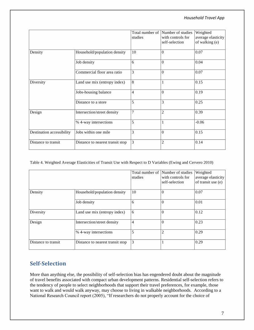
Next we consider the D variables that influence walking. The meta-analysis shows that mode share and

likelihood of walk trips are most strongly associated with the design and diversity dimensions of built

environments. Intersection density, jobs-housing balance, and distance to stores have the greatest

elasticities. Interestingly, intersection density is a more significant variable than street connectivity.

Intuitively this seems right, as walkability may be limited even if connectivity is excellent when blocks

are long. Also of interest is the fact that jobs-housing balance has a stronger relationship to walking than

the more commonly used land use mix (entropy) variable. Several variables that often go hand-in-hand

with population density have elasticities that are well above that of population density. Also, as with

VMT, job density is less strongly related to walking than is population density. Table 2 suggests that

having transit stops nearby may stimulate walking.

Finally, we consider the D variables that influence transit use (see Table 3). The mode share and

likelihood of transit trips are strongly associated with transit access. Living near a bus stop appears to be

an inducement to ride transit, supporting the transit industry’s standard of running buses within a quarter

mile of most residents. Next in importance are road network variables and, then, measures of land use

mix. High intersection density and great street connectivity shorten access distances, and provide more

routing options for transit users and transit service providers. Land use mix makes it possible to

efficiently link transit trips with errands on the way to and from transit stops. It is sometimes said that


6

“mass transit needs ‘mass’”, however this is not supported by the low elasticities of transit use with

respect to population and job densities in Table 3.

No clear pattern emerges from scanning across Tables 2 through 4. Perhaps what can be said with the

highest degree of confidence is that destination accessibility is most strongly related to both motorized

(i.e., VMT) and non-motorized (i.e., walking) travel and that among the remaining Ds, density has the

weakest association with travel choices. The primacy of destination accessibility may be due to lower

levels of auto ownership and auto dependence at central locations. Almost any development in a central

location is likely to generate less automobile travel than the best-designed, compact, mixed-use

development in a remote location.

The relatively weak relationships between density and travel likely indicate that density is an intermediate

variable that is often expressed by the other Ds (i.e., dense settings commonly have mixed uses, short

blocks, and central locations, all of which shorten trips and encourage walking). Among design variables,

intersection density more strongly sways the decision to walk than does street connectivity. And among

diversity variables, jobs-housing balance is a stronger predictor of walk mode choice than land-use mix

measures. Linking where people live and work allows more to commute by foot, and this appears to shape

mode choice more than sprinkling multiple land uses around a neighborhood.

Table 2. Weighted Average Elasticities of VMT with Respect to D Variables (Ewing and Cervero 2010)

Total number

of studies

Number of studies with

controls for self-selection

Weighted average

elasticity of VMT (e)

Density Household/population

density

9 1 -0.04

Job density 5 1 0.00

Diversity Land use mix (entropy

index)

10 0 -0.09

Jobs-housing balance 4 0 -0.02

Design Intersection/street density 6 0 -0.12

% 4-way intersections 3 1 -0.12

Destination

accessibility

Job accessibility by auto 5 0 -0.20

Job accessibility by

transit

3 0 -0.05

Distance to downtown 3 1 -0.22

Distance to transit Distance to nearest transit

stop

6 1 -0.05

Table 3. Weighted Average Elasticities of Walking with Respect to D Variables (Ewing and Cervero 2010)


7

Total number of

studies

Number of studies

with controls for

self-selection

Weighted

average elasticity

of walking (e)

Density Household/population density 10 0 0.07


Commercial floor area ratio 3 0 0.07

Diversity Land use mix (entropy index) 8 1 0.15

Jobs-housing balance 4 0 0.19

Distance to a store 5 3 0.25

Design Intersection/street density 7 2 0.39

% 4-way intersections 5 1 -0.06

Destination accessibility Jobs within one mile 3 0 0.15

Distance to transit Distance to nearest transit stop 3 2 0.14

Table 4. Weighted Average Elasticities of Transit Use with Respect to D Variables (Ewing and Cervero 2010)

Total number of

studies

Number of studies

with controls for

self-selection

Weighted

average elasticity

of transit use (e)

Density Household/population density 10 0 0.07


Diversity Land use mix (entropy index) 6 0 0.12

Design Intersection/street density 4 0 0.23

% 4-way intersections 5 2 0.29

Distance to transit Distance to nearest transit stop 3 1 0.29

Self-Selection

More than anything else, the possibility of self-selection bias has engendered doubt about the magnitude

of travel benefits associated with compact urban development patterns. Residential self-selection refers to

the tendency of people to select neighborhoods that support their travel preferences, for example, those

want to walk and would walk anyway, may choose to living in walkable neighborhoods. According to a

National Research Council report (2005), “If researchers do not properly account for the choice of


8

neighborhood, their empirical results will be biased in the sense that features of the built environment

may appear to influence activity more than they in fact do. (Indeed, this single potential source of

statistical bias casts doubt on the majority of studies on the topic to date.)” (p. 5-7)

At least 38 studies using nine different research approaches have attempted to control for residential self-

selection (Mokhtarian & Cao, 2008; Cao, Mokhtarian, & Handy, 2009a). Nearly all of them found

“resounding” evidence of statistically significant associations between the built environment and travel

behavior, independent of self-selection influences (Cao, Mokhtarian, et al. 2009a, p. 389). However,

nearly all of them also found that residential self-selection attenuates the effects of the built environment

on travel.

We have no ability to control for residential self-selection in the multi-region study that follows, as most

of the underlying household surveys do not ask relevant attitudinal questions. But this may not be a

major limitation. In Ewing and Cervero (2010), controls for residential self-selection appear to increase

the absolute magnitude of elasticities if they have any effect at all. There may be good explanations for

this unexpected result. In a region with few pedestrian- and transit-friendly neighborhoods, residential

self-selection likely matches individual preferences with place characteristics, increasing the effect of the

D variables, a possibility posited by Lund et al. (2006, p. 256).

“. . . if people are simply moving from one transit-accessible location to another (and they use transit

regularly at both locations), then there is theoretically no overall increase in ridership levels. If, however,

the resident was unable to take advantage of transit service at their prior residence, then moves to a TOD

(transit-oriented development) and begins to use the transit service, the TOD is fulfilling a latent demand

for transit accessibility and the net effect on ridership is positive.”

Similarly, Chatman (2009, p. 1087) hypothesizes that “Residential self-selection may actually cause

underestimates of built environment influences, because households prioritizing travel access—

particularly, transit accessibility—may be more set in their ways, and because households may not find

accessible neighborhoods even if they prioritize accessibility.” He carries out regressions that explicitly

test for this, and finds that self-selection is more likely to enhance than diminish built environmental

influences.

Still, we are left with a question. Most of the literature reviewed by Cao, Mokhtarian, et al. (2009a) shows

that the effect of the built environment on travel is attenuated by controlling for self-selection, whereas

Ewing and Cervero (2010) find no effect (or enhanced effects) after controlling for self-selection. The

difference may lie in the different samples included in the two studies or in the crude way Ewing and

Cervero (2010) operationalized self-selection (lumping all studies that control for self-selection together

regardless of methodology).

Methods

This is a multivariate cross sectional study pooling household travel data and built environmental data

from six diverse regions of the United States. What distinguishes this study from the hundreds of earlier

studies is the external validity (generalizability) that comes with such a large and diverse database. A

study using data from, say, Portland OR or Houston TX could be challenged for relevance to other

regions of the country, particularly when different dependent and independent variables are used in each

study. A study that pools data from six diverse regions, and uses consistently defined built environmental

variables to predict several consistently defined travel outcome variables, should be ready for use in large

metropolitan areas across the U.S.

Data


9

A main criterion for inclusion of regions in this study was data availability. Regions had to offer:

regional household travel surveys with XY coordinates for trip ends, so we could geocode the

precise locations of residences and measure the precise lengths of trips; and

land use databases at the parcel level with detailed land use classifications, so we could study

land-use intensity and mix down to the parcel level.

Most U.S. regions fall short on one or both counts. While nearly all metropolitan planning organizations

(MPOs) have conducted regional household travel surveys as the basis for the calibration of regional

travel demand models, most have geo-coded trip ends only at the relatively coarse geography of traffic

analysis zones. Likewise, while most MPOs have historical land use databases that are used in model

calibration, these too provide data only for the relatively coarse geography of traffic analysis zones.

Traffic analysis zones vary in size from region to region, but as a general rule, are equivalent to census

block groups. They will ordinarily not coincide with relevant built environments for individual

households.

The regions included in our sample met both criteria, and in addition, were able to supply GIS data layers

for streets, transit stops, and population and employment at the traffic analysis zone level. Buffers were

established around household geocodes locations with three different buffer widths, ¼ mile, ½ mile, and 1

mile. Built environmental variables were computed for each household and all three buffer widths. The

rationale for using different buffers is that different travel outcomes may depend on the built environment

at different widths around home locations. For example, the number of walk trips may depend on

conditions within a short distance of the home location, while the number or length of vehicle trips may

depend on conditions over a larger area.

Regions, survey dates, and sample sizes are shown in Table 5. Not all variables were calculable for all

cases, so effective sample sizes are somewhat smaller. Still, to our knowledge, this is largest sample of

household travel records ever collected for such a study outside of the National Household Travel Survey.

And relative to NHTS, our database provides much larger samples for individual regions and permits that

calculation of wider array of built environmental variables for use in modeling travel outcomes.

Table 5. Regional Household and Trip Samples

Survey

Year

Surveyed

Households

Surveyed

Trips

Austin 2005 1,450 14,377

Boston 1991 2,599 20,756

Houston 1995 1,960 20,039

Portland 1994 3,832 50,574

Sacramento 2001 3,520 33,519

Seattle 2006 4,126 40,522

Total 17,487 179,787


10

Variables

The dependent and independent variables used in this study are defined in Table 6. Sample sizes and

descriptive statistics are also provided. Only the unlogged independent variables are shown in Table 6.

For each of them, there is a natural logged variable with the same variable name but for an “ln” at the

beginning (for example, hhsize and lnhhsize). The logged variables have the potential to account for

nonlinearity in the data set and to reduce the effect of outliers.

The variables in this app cover all of the Ds, from density to demographics. With different measures,

different buffer widths, and both absolute and logged variables, a total of 50 independent variables were

available to explain household travel outcomes. The variables were consistently defined across regions.

That is one of the main strengths of this study.

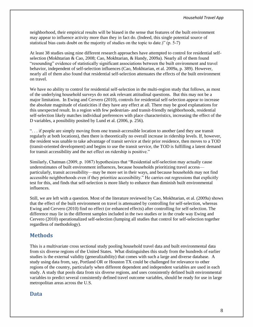
Table 6. Dependent and Independent Variables

variable description N Mean S.D.

dependent variables

posvmt positive household VMT (1=yes,

0=no)

17,487 0.91 0.29

vmt household VMT (for households with

positive VMT)

17,423 51.90 54.90

auto household private vehicle trips 17,424 8.33 7.38

walk household walk trips 17,424 0.90 2.13

bike household bike trips 17,424 0.13 0.78

transit household transit trips 17,424 0.26 0.93

independent variables – household

hhsize household size 17,484 2.15 1.21

hhworkers number employed 17,487 1.17 0.86

hhincome real household income (1973 dollars) 15,432 30,486.85 18,146.16

independent variables – buffers

actden1/4mi activity density quarter mile (pop +

emp per square mile)

16,854 16,217.05 30,531.49

jobpop1/4mi job-population balance quarter mile 16,853 0.54 0.28

entropy1/4mi land use entropy quarter mile 16,667 0.32 0.28

intden1/4mi intersection density quarter mile 17,252 202.63 133.71


11

int4w1/4mi percentage 4-way intersections quarter

mile

17,022 31.33 25.39

stopden1/4mi transit stop density quarter mile 17,252 38.00 57.00

actden1/2mi activity density half mile (pop + emp

per square mile)

17,087 13,630.93 22,142.57

jobpop1/2mi job-population balance half mile 17,078 0.55 0.28

entropy1/2mi land use entropy half mile 16,852 0.44 0.27

intden1/2mi intersection density half mile 17,270 178.80 115.09

int4w1/2mi percentage 4-way intersections half

mile

17,193 29.94 20.81

stopden1/2mi transit stop density half mile 17,270 31.67 38.43

actden1mi activity density one mile (pop + emp

per square mile)

17,157 12,506.68 18,487.08

jobpop1mi job-population balance one mile 17,156 0.60 0.26

entropy1mi land use entropy one mile 16,902 0.52 0.25

intden1mi intersection density one mile 17,290 162.83 102.44

int4w1mi percentage 4-way intersections one

mile

17,229 29.29 18.03

stopden1mi transit stop density one mile 17,290 26.86 30.56

rail1/2mi rail station within one half mile (1=yes,

0=no)

17,450 0.25 2.21

emp10mina percentage of regional employment

within 10 minutes by auto

17,156 7.70 9.08



17,159 30.56 23.64



17,159 54.15 29.54

emp30mint percentage of regional employment


17,286 12.58 18.08

Statistical Analysis


12

To increase statistical power and external validity, we are pooling household travel data from six diverse

regions. Our data and model structure are hierarchical, with households nested within regions.

The solution to the problem of nested data is multilevel modeling (MLM), also called hierarchical

modeling (HLM). MLM modeling is just beginning to be used in the planning field (Ewing et al. 2011).

MLM accounts for dependence among observations, in this case the dependence of households within a

given region. All households within a given region share the characteristics of that region. This

dependence violates the independence assumption of ordinary least squares ("OLS") regression. Standard

errors of regression coefficients based on OLS will consequently be underestimated. Moreover, OLS

coefficient estimates will be inefficient. MLM overcomes these limitations, accounting for the

dependence among observations and producing more accurate coefficient and standard error estimates

(Raudenbush and Bryk 2002).

Regions such as Boston and Houston are likely to generate very different travel patterns irrespective of

household characteristics. The essence of MLM is to isolate the variance associated with each data level.

Despite the small number of Level 2 units (six regions) in this study, we can partition variance between

the household level (Level 1) and the region level (Level 2). However, we cannot reliably explain Level

2 variance with Level 2 variables when the sample is this small. Variables such as regional population

and density are unlikely to prove statistically significant predictors of household travel due to limited

degrees of freedom. As the number of regions increases, we would expect Level 2 variables to gain

statistical significance. It is our intent to eventually pool data from at least 10 different regions.

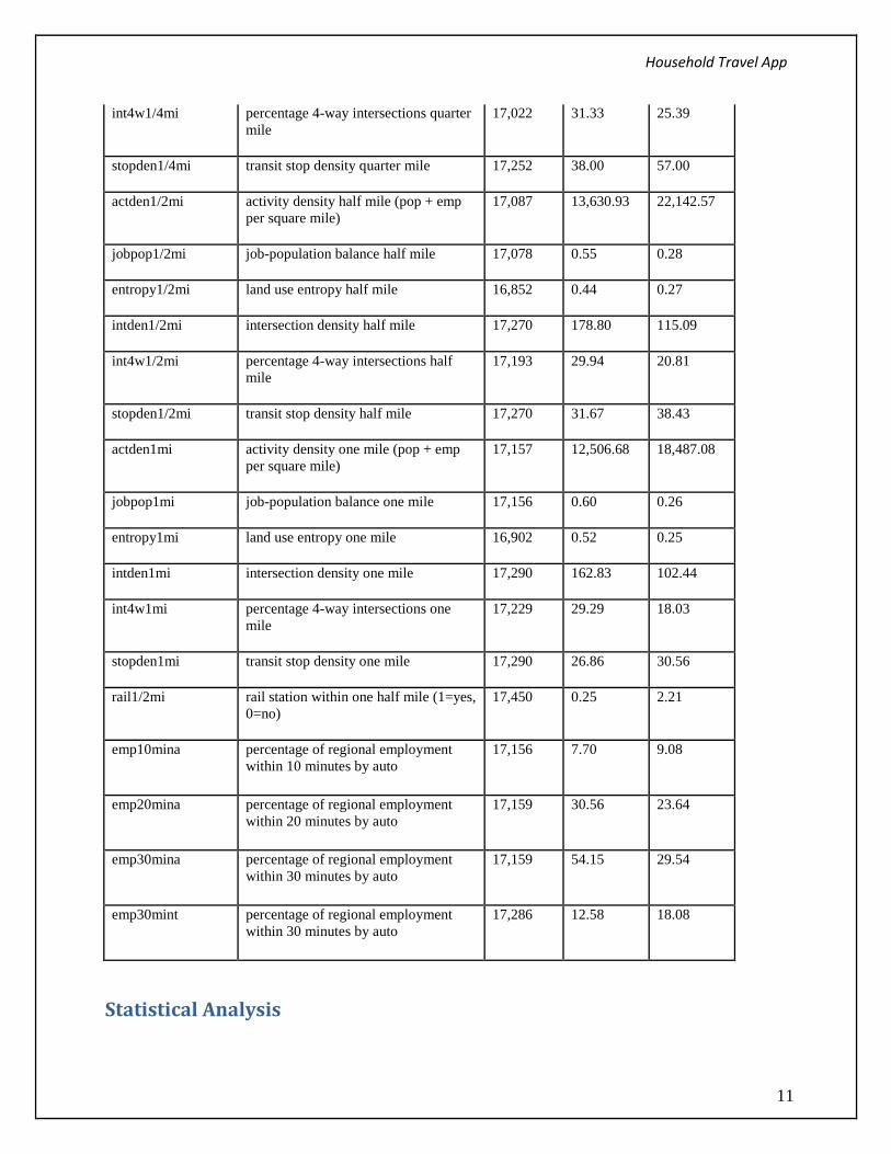
The dependent variables are of two types: continuous (VMT per household) and counts (vehicle trips,

walk trips, and transit trips). VMT per household has two characteristics that complicate the modeling of

it. First, it is non-normally distributed (see Figure 1). The solution to this problem is to take the natural

logarithm of VMT, which becomes our dependent variable (see Figure 2). Second, it has a large number

of zero values for households that generate no VMT. These households only use alternative modes such

as transit or walking. About one in 10 households in the sample fall into this category. When VMT is log

transformed, these households have undefined values of the dependent variable.

The solution to this problem is to estimate a two-stage “hurdle” model of VMT per household (Greene

2012, pp. 443, 824-826). We are aware of no previous application of hurdle models to the planning field.

The stage 1 model categorizes households as either generating positive VMT or not, and the stage 2

model estimates the amount of VMT generated for those categorized as generating VMT. “In some

settings, the zero outcome of the data generating process is qualitatively different from the positive ones.

The zero or nonzero values of the outcome is the result of a separate decision whether or not to

‘participate’ in the activity. On deciding to participate, the individual decides separately how much to,

that is, how intensively [to participate]” (Greene, 2012, p. 824).

Figure 1. Histogram of VMT per Household vs. a Normal Distribution


13

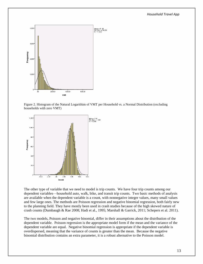
Figure 2. Histogram of the Natural Logarithim of VMT per Household vs. a Normal Distribution (excluding

households with zero VMT)

The other type of variable that we need to model is trip counts. We have four trip counts among our

dependent variables—household auto, walk, bike, and transit trip counts. Two basic methods of analysis

are available when the dependent variable is a count, with nonnegative integer values, many small values

and few large ones. The methods are Poisson regression and negative binomial regression, both fairly new

to the planning field. They have mostly been used in crash studies because of the high skewed nature of

crash counts (Dumbaugh & Rae 2008; Hadi et al., 1995; Marshall & Garrick, 2011; Schepers et al. 2011).

The two models, Poisson and negative binomial, differ in their assumptions about the distribution of the

dependent variable. Poisson regression is the appropriate model form if the mean and the variance of the

dependent variable are equal. Negative binomial regression is appropriate if the dependent variable is

overdispersed, meaning that the variance of counts is greater than the mean. Because the negative

binomial distribution contains an extra parameter, it is a robust alternative to the Poisson model.


14

“A central distributional assumption of the Poisson model is the equivalence of the Poisson mean and

variance. This assumption is rarely met with real data. Usually the variance exceeds the mean, resulting in

what is termed overdispersion… Overdispersion is, in fact, the norm and gives rise to a variety of other

models that are extensions of the basic Poisson model. Negative binomial regression is nearly always

thought of as the model to be used instead of Poisson when overdispersion is present in the data” (Hilbe,

2011, pg. 140).

Popular indicators of overdispersion are the Pearson and χ2 statistics divided by the degrees of freedom,

so-called dispersion statistics. If these statistics are greater than 1.0, a model is said to be overdispersed

(Hilbe, 2011, pp. 88, 142). By these measures, we have overdispersion of trip counts in our data set, and

the negative binomial model is more appropriate than the Poisson model.

Results

There is no theoretically superior model involving different D variables and different buffer widths.

Theoretically, buffers could be wide or narrow. Even a determinant as straightforward as walking

distance could be anywhere from one quarter mile to one mile. Relationships may be linear (suggesting

linear variables) or nonlinear (suggesting logarithmic variables). Different Ds may emerge as significant

in different models. So trial and error was used to arrive at the best-fit models for the travel outcomes of

interest. Variables were substituted into models to see if they were statistically significant and improved

goodness-of-fit. For each dependent variable, we were looking for the model with the most significant t-

statistics and the highest pseudo-R2.

The best-fit model for the dichotomous variable, positive VMT (1=yes, 0=no), is presented in Table 7.

The likelihood of positive VMT increases with household size, number of employed household members,

and real household income. These sociodemographics are associated with increased likelihood of

vehicular travel. The likelihood of positive VMT declines with land use entropy within a quarter mile

buffer around the household, with the percentage of 4-way intersections within a half mile, with transit

stop density within a half mile, with activity density within a mile, and with intersection density within a

mile. All variables are significant at the 0.001 level or beyond, except intersection density which is

significant at the 0.002 level. Basically, those who live in highly accessible places (characterized by these

five D variables) are better able to make do without vehicle trips. However, the probability of positive

VMT remains high for all cohorts. The pseudo-R2 of this model only 0.15, suggesting that much of the

variance in this dichotomous variable remains unexplained.

Table 7. Logistic Regression Model of Log Odds of Positive Household VMT

coeff std error t-ratio p-value

constant -4.40 0.522 -8.44 <0.001

lnhhsize 0.755 0.082 9.26 <0.001

hhworkers 0.343 0.055 6.29 <0.001

lnhhincome 0.771 0.045 17.2 <0.001

lnentropy1/4mi -0.744 0.128 -5.81 <0.001


15

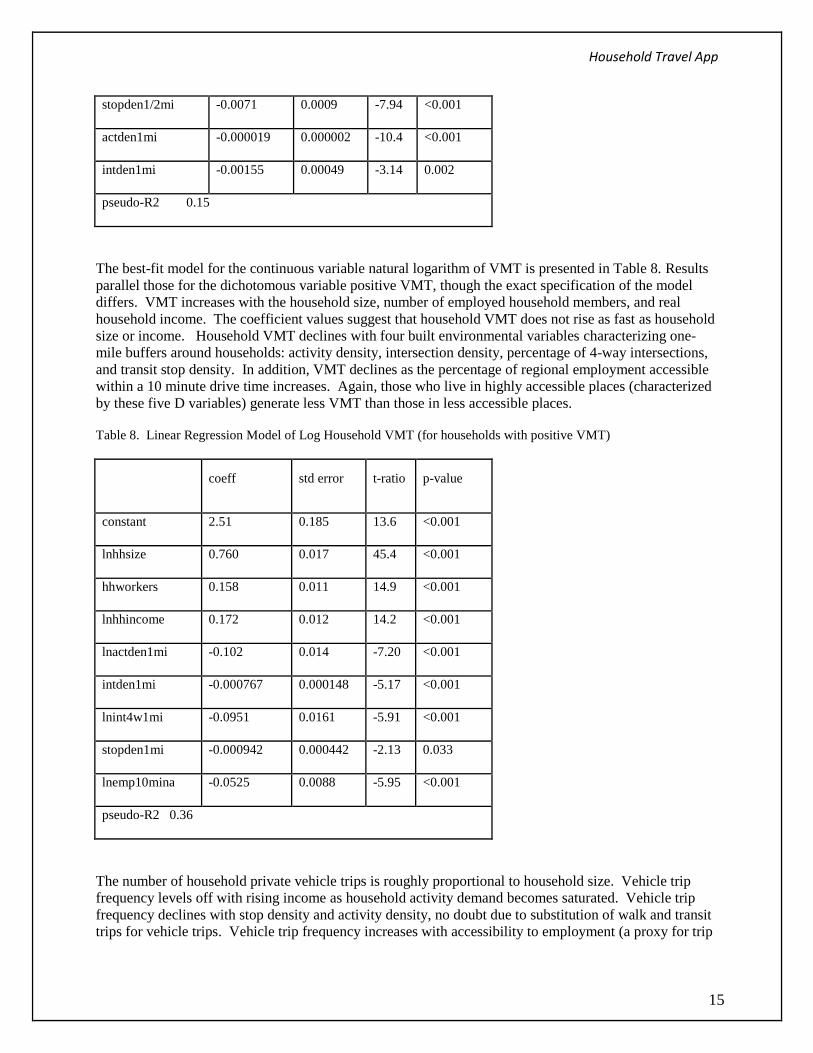
stopden1/2mi -0.0071 0.0009 -7.94 <0.001

actden1mi -0.000019 0.000002 -10.4 <0.001

intden1mi -0.00155 0.00049 -3.14 0.002

pseudo-R2 0.15

The best-fit model for the continuous variable natural logarithm of VMT is presented in Table 8. Results

parallel those for the dichotomous variable positive VMT, though the exact specification of the model

differs. VMT increases with the household size, number of employed household members, and real

household income. The coefficient values suggest that household VMT does not rise as fast as household

size or income. Household VMT declines with four built environmental variables characterizing one-

mile buffers around households: activity density, intersection density, percentage of 4-way intersections,

and transit stop density. In addition, VMT declines as the percentage of regional employment accessible

within a 10 minute drive time increases. Again, those who live in highly accessible places (characterized

by these five D variables) generate less VMT than those in less accessible places.

Table 8. Linear Regression Model of Log Household VMT (for households with positive VMT)


constant 2.51 0.185 13.6 <0.001

lnhhsize 0.760 0.017 45.4 <0.001

hhworkers 0.158 0.011 14.9 <0.001

lnhhincome 0.172 0.012 14.2 <0.001

lnactden1mi -0.102 0.014 -7.20 <0.001

intden1mi -0.000767 0.000148 -5.17 <0.001

lnint4w1mi -0.0951 0.0161 -5.91 <0.001

stopden1mi -0.000942 0.000442 -2.13 0.033

lnemp10mina -0.0525 0.0088 -5.95 <0.001

pseudo-R2 0.36

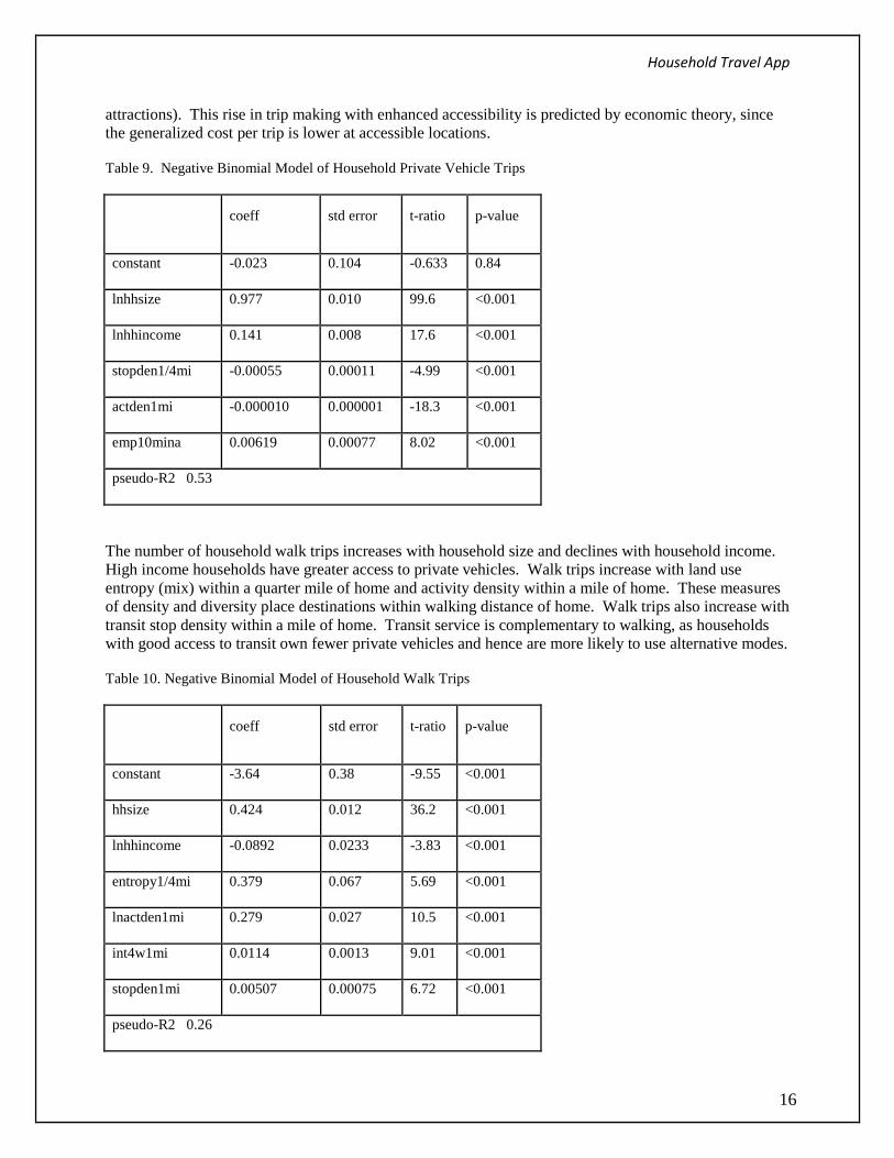
The number of household private vehicle trips is roughly proportional to household size. Vehicle trip

frequency levels off with rising income as household activity demand becomes saturated. Vehicle trip

frequency declines with stop density and activity density, no doubt due to substitution of walk and transit

trips for vehicle trips. Vehicle trip frequency increases with accessibility to employment (a proxy for trip


16

attractions). This rise in trip making with enhanced accessibility is predicted by economic theory, since

the generalized cost per trip is lower at accessible locations.

Table 9. Negative Binomial Model of Household Private Vehicle Trips


constant -0.023 0.104 -0.633 0.84

lnhhsize 0.977 0.010 99.6 <0.001

lnhhincome 0.141 0.008 17.6 <0.001

stopden1/4mi -0.00055 0.00011 -4.99 <0.001

actden1mi -0.000010 0.000001 -18.3 <0.001

emp10mina 0.00619 0.00077 8.02 <0.001

pseudo-R2 0.53

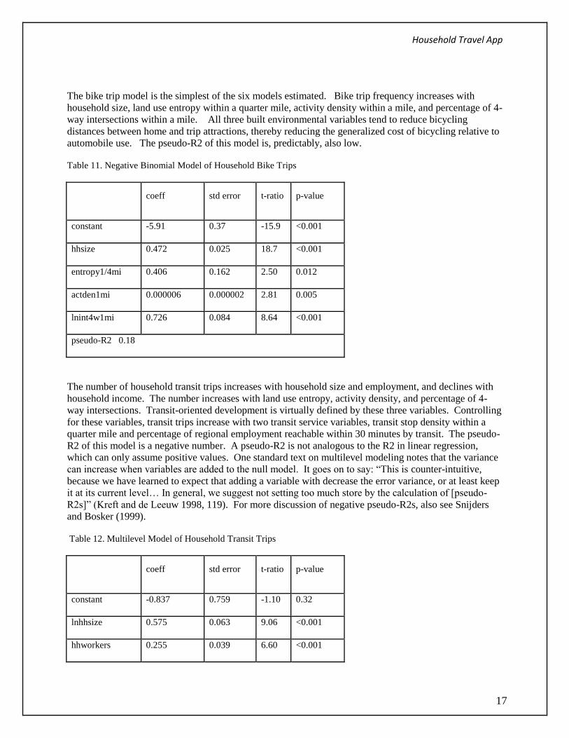
The number of household walk trips increases with household size and declines with household income.

High income households have greater access to private vehicles. Walk trips increase with land use

entropy (mix) within a quarter mile of home and activity density within a mile of home. These measures

of density and diversity place destinations within walking distance of home. Walk trips also increase with

transit stop density within a mile of home. Transit service is complementary to walking, as households

with good access to transit own fewer private vehicles and hence are more likely to use alternative modes.

Table 10. Negative Binomial Model of Household Walk Trips


constant -3.64 0.38 -9.55 <0.001

hhsize 0.424 0.012 36.2 <0.001

lnhhincome -0.0892 0.0233 -3.83 <0.001

entropy1/4mi 0.379 0.067 5.69 <0.001

lnactden1mi 0.279 0.027 10.5 <0.001

int4w1mi 0.0114 0.0013 9.01 <0.001

stopden1mi 0.00507 0.00075 6.72 <0.001

pseudo-R2 0.26


17

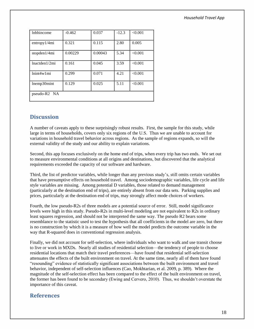
The bike trip model is the simplest of the six models estimated. Bike trip frequency increases with

household size, land use entropy within a quarter mile, activity density within a mile, and percentage of 4-

way intersections within a mile. All three built environmental variables tend to reduce bicycling

distances between home and trip attractions, thereby reducing the generalized cost of bicycling relative to

automobile use. The pseudo-R2 of this model is, predictably, also low.

Table 11. Negative Binomial Model of Household Bike Trips


constant -5.91 0.37 -15.9 <0.001

hhsize 0.472 0.025 18.7 <0.001

entropy1/4mi 0.406 0.162 2.50 0.012

actden1mi 0.000006 0.000002 2.81 0.005

lnint4w1mi 0.726 0.084 8.64 <0.001

pseudo-R2 0.18

The number of household transit trips increases with household size and employment, and declines with

household income. The number increases with land use entropy, activity density, and percentage of 4-

way intersections. Transit-oriented development is virtually defined by these three variables. Controlling

for these variables, transit trips increase with two transit service variables, transit stop density within a

quarter mile and percentage of regional employment reachable within 30 minutes by transit. The pseudo-

R2 of this model is a negative number. A pseudo-R2 is not analogous to the R2 in linear regression,

which can only assume positive values. One standard text on multilevel modeling notes that the variance

can increase when variables are added to the null model. It goes on to say: “This is counter-intuitive,

because we have learned to expect that adding a variable with decrease the error variance, or at least keep

it at its current level… In general, we suggest not setting too much store by the calculation of [pseudo-

R2s]” (Kreft and de Leeuw 1998, 119). For more discussion of negative pseudo-R2s, also see Snijders

and Bosker (1999).

Table 12. Multilevel Model of Household Transit Trips


constant -0.837 0.759 -1.10 0.32

lnhhsize 0.575 0.063 9.06 <0.001

hhworkers 0.255 0.039 6.60 <0.001


18

lnhhincome -0.462 0.037 -12.3 <0.001

entropy1/4mi 0.321 0.115 2.80 0.005

stopden1/4mi 0.00229 0.00043 5.34 <0.001

lnactden1/2mi 0.161 0.045 3.59 <0.001

lnint4w1mi 0.299 0.071 4.21 <0.001

lnemp30mint 0.129 0.025 5.11 <0.001

pseudo-R2 NA

Discussion

A number of caveats apply to these surprisingly robust results. First, the sample for this study, while

large in terms of households, covers only six regions of the U.S. Thus we are unable to account for

variations in household travel behavior across regions. As the sample of regions expands, so will the

external validity of the study and our ability to explain variations.

Second, this app focuses exclusively on the home end of trips, when every trip has two ends. We set out

to measure environmental conditions at all origins and destinations, but discovered that the analytical

requirements exceeded the capacity of our software and hardware.

Third, the list of predictor variables, while longer than any previous study’s, still omits certain variables

that have presumptive effects on household travel. Among sociodemographic variables, life cycle and life

style variables are missing. Among potential D variables, those related to demand management

(particularly at the destination end of trips), are entirely absent from our data sets. Parking supplies and

prices, particularly at the destination end of trips, may strongly affect mode choices of workers.

Fourth, the low pseudo-R2s of three models are a potential source of error. Still, model significance

levels were high in this study. Pseudo-R2s in multi-level modeling are not equivalent to R2s in ordinary

least squares regression, and should not be interpreted the same way. The pseudo R2 bears some

resemblance to the statistic used to test the hypothesis that all coefficients in the model are zero, but there

is no construction by which it is a measure of how well the model predicts the outcome variable in the

way that R-squared does in conventional regression analysis.

Finally, we did not account for self-selection, where individuals who want to walk and use transit choose

to live or work in MXDs. Nearly all studies of residential selection—the tendency of people to choose

residential locations that match their travel preferences—have found that residential self-selection

attenuates the effects of the built environment on travel. At the same time, nearly all of them have found

“resounding” evidence of statistically significant associations between the built environment and travel

behavior, independent of self-selection influences (Cao, Mokhtarian, et al. 2009, p. 389). Where the

magnitude of the self-selection effect has been compared to the effect of the built environment on travel,

the former has been found to be secondary (Ewing and Cervero, 2010). Thus, we shouldn’t overstate the

importance of this caveat.

References


19

Babisch, W. (2008). Road traffic noise and cardiovascular risk. Noise & Health, 10(38), 27-33.

Badland, H., & Schofield, G. (2005). Transport, urban design, and physical activity: An evidence-based

update. Transportation Research D, 10(3), 177-196.

Badoe, D. A. & Miller, E. J. (2000). Transportation–land-use interaction: Empirical findings in North

America, and the implications for modeling. Transportation Research D, 5(4), 235-263.

Bagley, M., & Mokhtarian, P. (2002). The impact of residential neighborhood type on travel behavior: A

structural equations modeling approach. Annals of Regional Science, 36(2), 279-297.

Bartholomew, K., & Ewing, R. (2008). Land use-transportation scenarios and future vehicle travel and

land consumption: A meta-analysis. Journal of the American Planning Association, 75(1), 1-15.

Bauman, A. E., & Bull, F. C. (2007). Environmental correlates of physical activity and walking in adults

and children: A review of reviews. London, U.K.: National Institute of Health and Clinical Excellence.

Bento, A. M., Cropper, M. L., Mobarak, A. M., & Vinha, K. (2003). The impact of urban spatial structure

on travel demand in the United States. (World Bank policy research working paper #3007).

Besser, L., & Dannenberg, A. (2005). Walking to public transit: Steps to help meet physical activity

recommendations. American Journal of Preventive Medicine, 29(4), 273-280.

Bhatia, R. (2004, June). Land use: A key to livable transportation. Paper presented at the 40th

International Making Cities Livable conference, London.

Bhat, C.R., and J.Y. Guo (2007), "A Comprehensive Analysis of Built Environment Characteristics on

Household Residential Choice and Auto Ownership Levels" Transportation Research Part B, Vol. 41, No.

5, pp. 506-526

Bhat, C.R., and N. Eluru (2009), "A Copula-Based Approach to Accommodate Residential Self-Selection

Effects in Travel Behavior Modeling," Transportation Research Part B, Vol. 43, No. 7, pp. 749-765,

Bhat, C.R., S. Sen, and N. Eluru (2009), "The Impact of Demographics, Built Environment Attributes,

Vehicle Characteristics, and Gasoline Prices on Household Vehicle Holdings and Use," Transportation

Research Part B, Vol. 43, No. 1, pp. 1-18, 2009

Boarnet, M. G., & Sarmiento, S. (1998). Can land-use policy really affect travel behavior? A study of the

link between non-work travel and land-use characteristics. Urban Studies, 35(7), 1155-1169.

Boarnet, M. G., & Greenwald, M. (2000). Land use, urban design, and non-work travel: Reproducing for

Portland, Oregon empirical tests from other urban areas. Transportation Research Record, 1722, 27-37.

Boarnet, M. G., & Crane, R. (2001). The influence of land use on travel behavior: Specification and

estimation strategies. Transportation Research A, 35(9), 823-845.

Boarnet, M. G., Nesamani, K. S., & Smith, C. S.(2004, January). Comparing the influence of land use on

nonwork trip generation and vehicle distance traveled: An analysis using travel diary data. Paper

presented at the 83rd annual meeting of the Transportation Research Board, Washington, DC.

Boarnet, M. G., Greenwald, M., & McMillan, T. (2008). Walking, urban design, and health: Toward a

cost-benefit analysis framework. Journal of Planning Education and Research, 27(3), 341-358.

mip://0221f4a8/default.html??

mip://0221f4a8/default.html??

http://www.ce.utexas.edu/prof/bhat/Copula.html

http://www.ce.utexas.edu/prof/bhat/Copula.html


20

Boarnet, M. G., Joh, K., Siembab, W., Fulton, W., & Nguyen, M. T. (2009). Transportation planning in

an era of expensive mobility. Unpublished manuscript.

Borenstein, M., Hedges, L.V., Higgins, J. P. T., & Rothstein, H. R. (2009). Introduction to meta-analysis.

Chichester, U.K.: Wiley.

Bunn, F., Collier, T., Frost, C., Ker, K., Roberts, I. & Wentz, R. (2003). Traffic calming for the

prevention of road traffic injuries: Systematic review and meta-analysis. Injury Prevention, 9(3), 200-204.

Button, K. & Kerr, J. (1996). Effectiveness of traffic restraint policies: A simple meta-regression analysis.

International Journal of Transport Economics, 23, 213-225.

Button, K. & Nijkamp, P. (1997). Environmental policy analysis and the usefulness of meta-analysis.

Socio-Economic Planning Sciences, 31(3), 231-240.

Cao, X. (2010). Exploring causal effects of neighborhood type on walking behavior using stratification on

the propensity score. Environment and Planning A, 42(2), 487-504.

Cao, X., Handy, S. L., & Mokhtarian, P. L. (2006). The influences of the built environment and

residential self-selection on pedestrian behavior: Evidence from Austin, TX. Transportation, 33(1), 1-20.

Cao, X., Mokhtarian, P. L., & Handy, S. L. (2007). Do changes in neighborhood characteristics lead to

changes in travel behavior? A structural equations modeling approach. Transportation, 34(5). 535-556.

Cao, X., Mokhtarian, P. L., & Handy, S. L. (2009a). Examining the impacts of residential self-selection

on travel behaviour: A focus on empirical findings. Transport Reviews, 29(3), 359-395.

Cao, X., Mokhtarian, P. L. & Handy, S. L. (2009b). The relationship between the built environment and

nonwork travel: A case study of northern California. Transportation Research Part A, 43(5), 548-559.

Cao, X., Xu, Z., & Fan, Y. (2009, January). Exploring the connections among residential location, self-

selection, and driving behavior: A case study of Raleigh, NC. Paper presented at the 89th annual meeting

of the Transportation Research Board.

Cervero, R. (2001). Walk-and-ride: Factors influencing pedestrian access to transit. Journal of Public

Transportation, 3(4), 1-23.

Cervero, R. (2002a). Built environments and mode choice: Toward a normative framework.

Transportation Research D, 7(4), 265-284.

Cervero, R. (2002b). Induced travel demand: Research design, empirical evidence, and normative

policies. Journal of Planning Literature, 17(1), 3-20.

Cervero, R. (2003). The built environment and travel: Evidence from the United States. European Journal

of Transport and Infrastructure Research, 3(2), 119-137.

Cervero, R. (2006). Alternative approaches to modeling the travel-demand impacts of smart growth.

Journal of the American Planning Association, 72(3), 285-295.

Cervero, R. (2007). Transit oriented development's ridership bonus: A product of self-selection and public

policies. Environment and Planning Part A, 39(9), 2068-2085.


21

Cervero, R., & Duncan, M. (2003). Walking, bicycling, and urban landscapes: Evidence from the San

Francisco Bay Area. American Journal of Public Health, 93(9), 1478-1483.

Cervero, R., & Duncan, M. (2006). Which reduces vehicle travel more: Jobs-housing balance or retail-

housing mixing? Journal of the American Planning Association, 72(4), 475-490.

Cervero, R., & Kockelman, K. (1997). Travel demand and the 3Ds: Density, diversity, and design.

Transportation Research D, 2(3), 199-219.

Cervero, R., & Murakami, J. (2010). Effects of built environments on vehicle miles traveled: Evidence

from 370 U.S. metropolitan areas, Environment and Planning A, 42(2) 400 – 418.

Chapman, J., & Frank, L. (2004). Integrating travel behavior and urban form data to address

transportation and air quality problems in Atlanta, Georgia (Research Project No. 9819, Task Order 97-

13). Washington, DC: U.S. Department of Transportation.

Chatman, D. G. (2003). How density and mixed uses at the workplace affect personal commercial travel

and commute mode choice. Transportation Research Record, 1831, 193-201.

Chatman, D. G. (2008) Deconstructing development density: Quality, quantity and price effects on

household non-work travel. Transportation Research Part A, 42(7), 1009–1031.

Chatman, D. G. (2009). Residential self-selection, the built environment, and nonwork travel: Evidence

using new data and methods. Environment and Planning A, 41(5), 1072–1089.

Chen, C. & McKnight, C. E. (2007). Does the built environment make a difference? Additional evidence

for the daily activity and travel behavior of homemakers living in New York City and suburb. Journal of

Transport Geography, 15(5), 380-395.

Craig, C. L, Brownson, R. C., Cragg, S. E., & Dunn, A. L. (2002). Exploring the effect of the

environment on physical activity: A study examining walking to work. American Journal of Preventive

Medicine, 23(2), 36-43.

Crane, R. (1996). On form versus function: Will the new urbanism reduce traffic, or increase it? Journal

of Planning Education and Research, 15(2), 117–126.

Crane, R. (2000). The influence of urban form on travel: An interpretive review. Journal of Planning

Literature, 15(1), 3-23.

Cunningham, G. O., & Michael, Y. L. (2004). Concepts guiding the study of the impact of the built

environment on physical activity for older adults: A review of the literature. American Journal of Health

Promotion, 18(6), 435-443.

Debrezion, G., Pels, E., & Rietveld, P. (2003). The impact of railway stations on residential and

commercial property value: A meta analysis. Tinbergen Institute Discussion Paper No. TI–2004–023/3.

Ding, D. & Gebel, K. (2012). Built environment, physical activity, and obesity: What have we learned

from reviewing the literature? Health & Place 18, 100–105.

DKS Associates. (2007). Assessment of local models and tools for analyzing smart-growth strategies:

Final report. Sacramento, CA: California Department of Transportation.


22

Duncan, M. J., Spence, J. C., & Mummery, W. K. (2005). Perceived environment and physical activity: a

meta-analysis of selected environmental characteristics. International Journal of Behavioral Nutrition and

Physical Activity, 2(11), doi:10.1186/1479-5868-2-11.

Edwards, R. D. (2008). Public transit, obesity, and medical costs: Assessing the magnitudes. Preventive

Medicine, 46(1),14-21.

Estupinan, N., & Rodriguez, D. A. (2008). The relationship between urban form and station boardings for

Bogota's BRT. Transportation Research A, 42(2), 296-306.

Ewing, R. (1996). Pedestrian and transit-friendly design. Tallahassee, FL: Florida Department of

Transportation.

Ewing, R., & Cervero, R. (2001). Travel and the built environment. Transportation Research Record,

1780, 87-114.

Ewing, R., DeAnna, M. & Li, S. (1996). Land use impacts on trip generation rates. Transportation

Research Record, 1518, 1-7.

Ewing, R., Greenwald, M. J., Zhang, M.,Walters, J., Feldman, M., Cervero, R., Frank, L. D., Thomas, J.

(2009). Measuring the impact of urban form and transit access on mixed use site trip generation rates –

Portland pilot study. Washington, DC: U.S. Environmental Protection Agency.

Ewing, R., Schroeer, W., Greene, W. (2004). School location and student travel: Analysis of factors

affecting mode choice. Transportation Research Record, 1895, 55-63.

Fan, Y. (2007). The built environment, activity space, and time allocation: An activity-based framework

for modeling the land use and travel connection. (Unpublished doctoral dissertation.) University of North

Carolina, Chapel Hill, NC.

Ferdinand, A.O., Sen, B., Rahurkar, S., Engler, S., and Menachemi, N. (2012). The Relationship Between

Built Environments and Physical Activity: A Systematic Review. American Journal of Public Health,

102(10), e7-e13.

Frank, L. D. (2000). Land use and transportation interaction: Implications on public health and quality of

life. Journal of Planning Education and Research, 20(1), 6-22.

Frank, L.D., & Engelke, P. (2001). The built environment and human activity patterns: Exploring the

impacts of urban form on public health. Journal of Planning Literature, 16(2), 202-218.

Frank, L. D., & Engelke, P. (2005). Multiple impacts of the built environment on public health: Walkable

places and the exposure to air pollution. International Regional Science Review, 28(2), 193-216.

Frank, L. D., Bradley, Kavage, S., Chapman, J., & Lawton, K. (2007) Urban form, travel time, and cost

relationships with tour complexity and mode choice. Transportation, 35(1), 37-54.

Frank, L. D., Kerr, J., Chapman, J., & Sallis, J. (2007). Urban form relationships with walk trip frequency

and distance among youth. American Journal of Health Promotion, 21(4), 305-311.

http://ntlsearch.bts.gov/tris/search.do?new=&b1=9&f1=au&t1=Rodriguez%2C+Daniel+A&d=tr

http://ntlsearch.bts.gov/tris/search.do?f1=mnid&new=&t1=387545&d=tr


23

Frank, L. D., Saelens, B. E., Powell, K. E., & Chapman, J. E. (2007). Stepping towards causation: Do

built environments or neighborhood and travel preferences explain physical activity, driving, and obesity?

Social Science & Medicine, 65(9),1898–1914.

Graham, D., & Glaister, S. (2002). Review of income and price elasticities of demand for road traffic.

London, U.K.: Centre for Transport Studies Imperial College of Science, Technology and Medicine.

Greenwald, M. J. (2009). SACSIM modeling –elasticity results: Draft. (Unpublished manuscript.) Walnut

Creek, CA: Fehr & Peers Associates.

Greenwald, M. J., & Boarnet, M. G. (2001). The built environment as a determinant of walking behavior:

Analyzing non-work pedestrian travel in Portland, Oregon. Transportation Research Record, 1780, 33-43.

Guo, J.Y., C.R. Bhat, and R.B. Copperman (2007), "Effect of the Built Environment on Motorized and

Non-Motorized Trip Making: Substitutive, Complementary, or Synergistic?," Transportation Research

Record, Vol. 2010, pp. 1-11, 2007,

Hamer, M., & Chida, Y. (2008) Active commuting and cardiovascular risk: A meta-analytic review.

Preventive Medicine, 46(1), 9-13.

Handy, S. L. (1993). Regional versus local accessibility: Implications for non-work travel. Transportation

Research Record, 1400, 58-66.

Handy, S. L. (2005). Critical assessment of the literature on the relationships among transportation, land

use, and physical activity. (Special Report 282: Does the built environment influence physical activity?

Examining the evidence.) Washington, DC: Transportation Research Board and Institute of Medicine

Committee on Physical Activity, Health, Transportation, and Land Use.

Handy, S. L., & Clifton, K. J. (2001). Local shopping as a strategy for reducing automobile travel.

Transportation, 28(4), 317-346.

Handy, S. L., Cao, X., & Mokhtarian, P. L. (2005). Correlation or causality between the built

environment and travel behavior? Evidence from Northern California. Transportation Research D, 10(6),

427-444.

Handy, S. L., Cao, X., & Mokhtarian, P. L. (2006). Self-selection in the relationship between the built

environment and walking—Empirical evidence from Northern California. Journal of the American

Planning Association, 72(1), 55-74.

Heath, G. W., Brownson, R. C., Kruger, J., Miles, R., Powell, K. E., Ramsey, L. T., & the Task Force on

Community Preventive Services. (2006). The effectiveness of urban design and land use and transport

policies and practices to increase physical activity: A systematic review. Journal of Physical Activity and

Health, 3(1), 55-76.

Hedel, R., & Vance, C. (2007, January). Impact of urban form on automobile travel: Disentangling

causation from correlation. Paper presented at the 86th annual meeting of the Transportation Research

Board, Washington, DC.

Hedges, L. V. & Olkin, I. (1985). Statistical methods for meta-analysis. Orlando, FL: Academic Press.

http://www.sciencedirect.com/science/journal/13619209


24

Hess, P. M., Moudon, A. V., Snyder, M. C., & Stanilov, K. (1999). Site design and pedestrian travel.

Transportation Research Record, 1674, 9-19.

Holtzclaw, J., Clear, R., Dittmar, H., Goldstein, D., & Haas, P. (2002). Location efficiency:

Neighborhood and socioeconomic characteristics determine auto ownership and use-studies in Chicago,

Los Angeles, and San Francisco. Transportation Planning and Technology, 25(1), 1-27.

Humpel, N., Owen, N., & Leslie, E. (2002). Environmental factors associated with adults’ participation in

physical activity: A review. American Journal of Preventative Medicine, 22(3), 188-199.

Hunter, J. E., & Schmidt, F.L. (2004). Methods of meta-analysis: Correcting error and bias in research

findings. Newbury Park, CA: Sage.

Joh, K., Boarnet, M. G, & Nguyen, M. T. (2009, January). Interactions between race/ethnicity, attitude,

and crime: Analyzing walking trips in the South Bay Area. Paper presented at the 88th annual meeting of

the Transportation Research Board, Washington, DC.

Johnston, R. (2004). The urban transportation planning process. In S. Hanson and G. Guiliano (Eds.), The

geography of urban transportation (pp. 115-140). New York, NY: Guilford Press.

Kahn, E. B., Ramsey, L. T., Brownson, R. C., Heath, G. W., & Howze, E. H. (2002). The effectiveness of

interventions to increase physical activity: A systematic review. American Journal of Preventive

Medicine, 22(4), 73-107.

Khattak, A. J., & Rodriquez, D. (2005). Travel behavior in neo-traditional neighborhood developments: A

case study in USA. Transportation Research A, 39(6), 481-500.

Kitamura, R., Mokhtarian, P. L., & Laidet, L. (1997). A micro-analysis of land use and travel in five

neighborhoods in San Francisco Bay Area. Transportation, 24(2), 125-158.

Kockelman, K. M. (1997). Travel behavior as a function of accessibility, land use mixing, and land use

balance: Evidence from the San Francisco Bay Area. Transportation Research Record, 1607, 116-125.

Krahnstoever-Davison, K., & Lawson, C. T. (2006). Do attributes in the physical environment influence

children's physical activity? A review of the literature. International Journal of Behavioral Nutrition and

Physical Activity, 3(19), doi: 10.1186/1479-5868-3-19.

Kuby, M., Barranda, A., & Upchurch, C. (2004). Factors influencing light-rail station boardings in the

United States. Transportation Research A, 38(3), 223-258.

Kuzmyak, R., Baber, C., & Savory, D. (2006). Use of a walk opportunities index to quantify local

accessibility. Transportation Research Record, 1977, 145-153.

Kuzmyak, R. (2009a). Estimating the travel benefits of blueprint land use concepts. (Unpublished

manuscript.) Los Angeles, CA: Southern California Association of Governments.

Kuzmyak, R. (2009b). Estimates of point elasticities. Phoenix, AZ: Maricopa Association of

Governments.

Lau, J., Ioannidis, J. P. A., Terrin, N., Schmid, C. H., & Olkin, I. (2006). The case of the misleading

funnel plot. British Medical Journal, 333( ), 597−600.


25

Lauria, M., & Wagner, J. A. (2006). What can we learn from empirical studies of planning theory? A

comparative case analysis of extant literature. Journal of Planning Education and Research, 25, 364-381.

Lawrence Frank & Company. (2009). I-PLACE3S Health & climate enhancements and their application

in King County. Seattle, WA: King County.

Leck, E. (2006). The impact of urban form on travel behavior: A meta-analysis. Berkeley Planning

Journal, 19, 37-58.

Lee, C., & Moudon, A. V. (2004). Physical activity and environment research in the health field:

Implications for urban and transportation planning practice and research. Journal of Planning Literature,

19, 147-181.

Lee, C., & Moudon, A. V. (2006a). Correlates of walking for transportation or recreation purposes.

Journal of Physical Activity and Health. 3(1), 77-98.

Lee, C., & Moudon, A.V. (2006b). The 3Ds + R: Quantifying land use and urban form correlates of

walking. Transportation Research Part D, 11, 204-215.

Li, F., Fisher, K. J., Brownson, R. C., & Bosworth, M. (2005). Multilevel modelling of built environment

characteristics related to neighbourhood walking activity in older adults. Journal of Epidemiology and

Community Health, 59(7), 558-564.

Lipsey, M. W., and Wilson, D. B. (2001). Practical meta-analysis. Thousand Oaks, CA: Sage.

Littell, J. H., Corcoran, J., & Pillai, V. (2008). Systematic reviews and meta-analysis. New York, NY:

Oxford University Press.

Livi Smith, A. D. (2009, January) Contribution of perception in analysis of walking behavior. Paper

presented at the 88th annual meeting of the Transportation Research Board, Washington, DC.

Lund, H. M. (2003). Testing the claims of new urbanism: Local access, pedestrian travel, and neighboring

behaviors. Journal of the American Planning Association, 69(4), 414-429.

Lund, H. M., Cervero, R., & Wilson, R. W. (2004). Travel characteristics of transit-oriented development

in California. Sacramento: California Department of Transportation.

Lund, H. M., Willson, R., & Cervero, R. (2006). A re-evaluation of travel behavior in California TODs.

Journal of Architectural and Planning Research, 23(3), 247-263.

Lyons, L. (2003). Meta–analysis: Methods of accumulating results across research domains. Retrieved

June 26, 2009, from http://www.lyonsmorris.com/MetaA

Macaskill, P., Walter, S. D., & Irwig, L. (2001). A comparison of methods to detect publication bias in

meta-analysis. Statistics in Medicine, 20(4), 641-654.

McCormack, G., Giles-Corti, B., Lange, A., Smith, T., Martin, K., & Pikora, T. J. (2004). An update of

recent evidence of the relationship between objective and self-report measures of the physical

environment and physical activity behaviours. Journal of Science and Medicine in Sport, 7(1), 81-92.

http://www.lyonsmorris.com/MetaA


26

McGinn, A. P., Evenson, K. E., Herring, A. H., Huston, S. L., & Rodriguez, D. A. (2007). Exploring

associations between physical activity and perceived and objective measures of the built

environment. Journal of Urban Health, 84(2), 162-184.

McMillan, T. E. (2005). Urban form and a child's trip to school: The current literature and a framework

for future research. Journal of Planning Literature, 19(4), 440-456.

McMillan T. E. (2007). The relative influence of urban form on a child's travel mode to school.

Transportation Research A, 41(1), 69-79.

Melo, P. C., Graham, D. J., & Noland, R. B. (2009). A meta-analysis of estimates of urban agglomeration

economies. Regional Science and Urban Economics, 39(3), 332-342.

Mokhtarian, P. L., & Cao, X. (2008). Examining the impacts of residential self-selection on travel

behavior: A focus on methodologies. Transportation Research B, 43(3), 204-228.

Næss, P. (2005). Residential location affects travel behavior—but how and why? The case of Copenhagen

metropolitan area. Progress in Planning, 63(1), 167–257.

National Research Council. (2005). Does the built environment influence physical activity? Examining

the evidence. (Special Report 282). Washington, DC: Transportation Research Board and Institute of

Medicine Committee on Physical Activity, Health, Transportation, and Land Use.

Nijkamp, P., & Pepping, G. (1998). A meta-analytical evaluation of sustainable city initiatives. Urban

Studies, 35(9), 1481-1500.

Newman, P. W. G., & Kenworthy, J. R. (2006). Urban design to reduce automobile dependence. Opolis:

An International Journal of Suburban and Metropolitan Studies, 2(1), 35-52.

Oakes, J. M., Forsyth, A., & Schmitz, K. H. (2007). The effects of neighborhood density and street

connectivity on walking behavior: The Twin Cities walking study. Epidemiologic Perspectives &

Innovations, 4(16), doi:10.1186/1742-5573-4-16.

Owen, N., Humpel, N., Leslie, E., Bauman, A., & Sallis, J. F. (2004). Understanding environmental

influences on walking: Review and research agenda. American Journal of Preventive Medicine, 27(1), 67-

76.

Pickrell, D., & Schimek, P. (1999). Growth in motor vehicle ownership and use: Evidence from the

Nationwide Personal Transportation Survey. Journal of Transportation and Statistics, 2(1), 1-17.

Pinjari, A.R., R.M. Pendyala, C.R. Bhat, and P.A. Waddell (2007a), "Modeling Residential Sorting

Effects to Understand the Impact of the Built Environment on Commute Mode Choice," Transportation,

Vol. 34, No. 5, pp. 557-573

Pinjari, A.R., R.M. Pendyala, C.R. Bhat, and P.A. Waddell (2007b), "Modeling the Choice Continuum:

An Integrated Model of Residential Location, Auto Ownership, Bicycle Ownership, and Commute Tour

Mode Choice Decisions," Technical paper, Department of Civil, Architectural & Environmental

Engineering, The University of Texas at Austin



27

Pinjari, A.R., N. Eluru, C.R. Bhat, R.M. Pendyala, and E. Spissu (2008), "Joint Model of Choice of

Residential Neighborhood and Bicycle Ownership: Accounting for Self-Selection and Unobserved

Heterogeneity," Transportation Research Record, Vol. 2082, pp. 17-26

Pinjari, A.R., C.R. Bhat, and D.A. Hensher (2009), "Residential Self-Selection Effects in an Activity

Time-use Behavior Model," Transportation Research Part B, Vol. 43, No. 7, pp. 729-748

Plaut, P. O. (2005). Non-motorized commuting in the U.S. Transportation Research D, 10(5), 347-356.

Pont, K., Ziviani, J., Wadley, D., Bennett, S., & Abbott, R. (2009). Environmental correlates of children’s

active transportation: A systematic literature review. Health & Place, 15(3), 827-840.

Pushkar, A. O., Hollingworth, B. J., & Miller, E. J. (2000, January). A multivariate regression model for

estimating greenhouse gas emissions from alternative neighborhood designs. Paper presented at the 79th

annual meeting of the Transportation Research Board, Washington, DC.

Rajamani, J., Bhat, C. R., Handy, S., Knaap, G., & Song, Y. (2003). Assessing the impact of urban form

measures in nonwork trip mode choice after controlling for demographic and level-of-service effects.

Transportation Research Record, 1831, 158-165.

Reilly, M. K. (2002, January). Influence of urban form and land use on mode choice: Evidence from the

1996 bay area travel survey. Paper presented at the 81st annual meeting of the Transportation Research

Board, Washington, DC.

Rodenburg, R., Benjamin, A., de Roos, C., Meijer, A. M. & Stams, G. J. (2009). Efficacy of EMDR in

children: A meta-analysis. Clinical Psychology Review, 29(7), 599-606.

Rodriguez, D. A., & Joo, J. (2004). The relationship between non-motorized mode choice and the local

physical environment. Transportation Research D, 9(2), 151-173.

Rose, M. (2004). Neighborhood design and mode choice. (Unpublished doctoral dissertation.) Portland,

OR: Portland State University.

Ross, C. L., & Dunning, A. E. (1997). Land use transportation interaction: An examination of the 1995

NPTS data. Washington, DC: U.S. Department of Transportation.

Rothstein, H. R., Sutton, A. J., & Borenstein, M. (2005). Publication bias in meta-analysis. In Rothstein,

H. R., Sutton, A. J. & Borenstein, M. (Eds.). Publication bias in meta-analysis: Prevention, assessment

and adjustment (pp. 1-7). Chichester, UK: Wiley.

Ryan, S. & Frank, L. D. (2009). Pedestrian Environments and Transit Ridership. Journal of Public

Transportation 12(1), 39-57.

Saelens, B. E., & Handy, S. (2008). Built environment correlates of walking: A review. Medicine &

Science in Sports & Exercise, 40(S), S550-S567.

Saelens, B. E., Sallis, J. F., & Frank, L. D. (2003). Environmental correlates of walking and cycling:

Findings from the transportation, urban design, and planning literatures. Annals of Behavioral Medicine,

25(2), 80-91.



28

Salon, D. (2006). Cars and the city: An investigation of transportation and residential location choices in

New York City. Davis, CA: Agricultural and Resource Economics, University of California, Davis.

Schimek, P. (1996). Household motor vehicle ownership and use: How much does residential density

matter? Transportation Research Record, 1552, 120-125.

Schulze, R. (2004). Meta-analysis: A comparison of approaches. Cambridge, MA: Hogrefe & Huber.

Shadish, W. R. & Haddock, C. K. (1994). Combining estimates of effect size. In Cooper, H. and Hedges,

L.V. (Eds.), The handbook of research synthesis (pp. 261-280). New York, NY: Russell Sage Foundation.

Shay, E., Fan, Y., Rodriguez, D. A., & Khattak, A. J. (2006). Drive or walk? Utilitarian trips within a

neo-traditional neighborhood. Transportation Research Record, 1985, 154-161.

Shay, E., & Khattak, A. J. (2005). Auto ownership and use in neotraditional and conventional

neighborhoods. Transportation Research Record, 1902, 18-25.

Shen, Q. (2000). Spatial and social dimensions of commuting. Journal of the American Planning

Association, 66(1), 68-82.

Smith, V. K. & Huang, J. (1995). Can markets value air quality? A meta-analysis of hedonic property

value models. Journal of Political Economy, 103(1): 209-227.

Soltani, A. & Allan, A. (2006). Analyzing the impacts of microscale urban attributes on travel: Evidence

from suburban Adelaide, Australia. Journal of Urban Planning and Development, 132(3), 132-137.

Stamps, A. E. III. (1990). Use of photographs to simulate environments: A meta-analysis. Perceptual and

Motor Skills, 71(3), 907-913.

Stamps, A. E. III. (1999). Demographic effects in environmental aesthetics: A meta-analysis. Journal of

Planning Literature, 14(2), 155-175.

Stead, D., & Marshall, S. (2001). The relationships between urban form and travel patterns. An

international review and evaluation. European Journal of Transport and Infrastructure Research, 1(2),

113-141.

Sun, X., Emany, M., Pendyala, R., & Wilmot, C. G. (1998). Household travel, household characteristics,

and land-use: An empirical study from the 1994 Portland travel survey. Transportation Research Record,

1617, 10-17.

Talvitie, A. (1976). Disaggregate travel demand models with disaggregate data, not with aggregate data,

and for what (Working Paper 7615). Berkeley, CA: Institute of Transportation Studies.

Targa, F., & Clifton, K. (2005). The built environment and trip generation for non-motorized travel.

Journal of Transportation and Statistics, 8(3), 55-70.

Tompa, E., de Oliveira, C., Dolinschi, R. & Irvin, E. (2008). A systematic review of disability

management interventions with economic evaluations. Journal of Occupational Rehabilitation, 18(1), 16-

26.

Train, K. (1986). Qualitative choice analysis: Theory, econometrics, and an application to automobile

demand. Cambridge, MA: The MIT Press.

http://www.ejtir.tudelft.nl/issues/2001_02/abstracts/2001_02_01.asp


29

Treadwell, J. R., Tregear, S. J., Reston, J. T., & Turkelson, C. H. (2006). A system for rating the stability

and strength of medical evidence. Medical Research Technology, 6(52) doi:10.1186/1471-2288-6-52.

Trost, S. G., Owen, N., Bauman, A. E., Sallis, J. F., Brown, W. (2002). Correlates of adults’ participation

in physical activity: Review and update. Medicine & Science in Sports & Exercise, 34(12), 1996-2001.

U.S. Environmental Protection Agency. (2004). Characteristics and performance of regional

transportation systems, (EPA-231-R-04-001). Washington, DC: Author.

van de Coevering, P., & Schwanen, T. (2006). Re-evaluating the impact of urban form on travel patterns

in Europe and North-America. Transport Policy, 13(3), 229-239.

Walters, J., Ewing, R., & Allen, E. (2000). Adjusting computer modeling tools to capture effects of smart

growth. Transportation Research Record, 1722, 17-26.

Waygood, E. O. D., Sun, Y., Kitamura, R. (2009, January). Children in transit oriented development:

Travel patterns, independence, and exercise. Paper presented at the 88th annual meeting of the

Transportation Research Board, Washington, DC.

Yarlagadda, A. K., & Srinivasan, S. (2008). Modeling children’s school travel mode and parental escort

decisions. Transportation, 35(2), 201-218.

Zegras, P. C. (2007). The built environment and motor vehicle ownership and use: Evidence from

Santiago de Chile. Paper presented at the 86th annual meeting of the Transportation Research Board,

Washington, DC.

Zhang, M. (2004). The role of land use in travel mode choice: Evidence from Boston and Hong Kong.

Journal of the American Planning Association, 70(3), 344-361.

Zhang, M. (2009, January). Bus vs. rail: A meta-analysis of cost characteristics, carrying capacities, and

land use impacts. Paper presented at the 88th annual meeting of the Transportation Research Board,

Washington, DC.

Zheng, Y. (2008). The benefit of public transportation: Physical activity to reduce obesity and ecological

footprint. Preventive Medicine, 46(1), 4-5.

Zhou, B., & Kockelman, K. (2008). Self-selection in home choice: Use of treatment effects in evaluating

relationship between built environment and travel behavior. Transportation Research Record, 2077, 54-

61.

http://ntlsearch.bts.gov/tris/search.do?new=&b1=9&f1=au&t1=Waygood%2C+E.+Owen+D&d=tr

http://ntlsearch.bts.gov/tris/search.do?new=&b1=9&f1=au&t1=Sun%2C+Yilin&d=tr

http://ntlsearch.bts.gov/tris/search.do?new=&b1=9&f1=au&t1=Kitamura%2C+Ryuichi&d=tr

http://ntlsearch.bts.gov/tris/search.do?new=&b1=9&f1=au&t1=Yarlagadda%2C+Amith+K&d=tr

http://ntlsearch.bts.gov/tris/search.do?new=&b1=9&f1=au&t1=Srinivasan%2C+Sivaramakrishnan&d=tr

household travel model - squarespace · household travel app 3 introduction some of today’s most...

Documents