household wealth and finances in germany: results …...life insurance policies are also included.2...

Household wealth and finances in Germany: results of the 2017 survey

Every three years, the Bundesbank conducts a survey of German households’ wealth and debt

entitled the “Panel on Household Finances (PHF)”. The collected data feed into studies of monet-

ary and financial stability policy and form the basis of research projects and analyses both within

and outside of the Bundesbank. Almost 5,000 households participated in the 2017 survey. Around

two- thirds of these households were taking part for the second or third time.

The results for 2017 show that household wealth increased on a broad front between 2014 and

2017. Both average net wealth and the median value increased significantly. The net wealth of

real estate owners, in particular, has risen owing to higher real estate prices. However, the wealth

of many tenant households and households in the poorer half of the distribution has also grown.

Higher incomes, in particular, are contributing to the positive wealth developments of these

households by putting them in a position to save more money and reducing their need to take

out new consumer loans.

Although some metrics of the inequality of wealth distribution declined slightly compared with

the previous survey, overall, no clear trend is evident in relation to earlier surveys.

The share of indebted households and the percentage of households with negative net wealth

changed only marginally between 2010 and 2017. The pressure on households from interest on

loans decreased during the same period. A much smaller share of indebted households’ income

was consumed by interest payments on loans in 2017 than in 2010.

This article describes the composition and distribution of household wealth and debt in Germany.

Other factors such as public finances, public pension provision, and access to education or the

healthcare system, to name just a few, also play a role when it comes to forming a more com-

prehensive assessment of the financial situation or indeed the welfare of households.

Deutsche Bundesbank Monthly Report

April 2019 13

Introduction

This article presents selected results of the 2017

survey on household wealth and finances in

Germany in 2017. As the Bundesbank had al-

ready conducted surveys on the wealth, debt

and income of households in Germany as well

as their saving and investment behaviour back

in 2010 and 2014, a comparison can also be

drawn across the years.

The present article limits itself to describing the

distribution and composition of households’

wealth. As a general rule, these statistics alone

do not allow any conclusions to be drawn

about possible causal relationships. Further an-

alysis is required for this. The study “Panel on

Household Finances (PHF)” was therefore de-

signed from the outset with a view to academic

research both within and outside of the Bun-

desbank. The anonymised microdatasets may

be requested from the Bundesbank’s Research

Data and Service Centre for academic research

projects. They are currently being used by over

200 researchers in more than 140 projects.

Wealth distribution in Germany in 2017

Wealth distribution can be characterised using

various statistical parameters. These include,

for example, the relationships between the

mean and median, Gini coefficients and

wealthy households’ share of total net wealth.

In order to calculate the ratio between mean

and median wealth, average (mean) wealth

must first be determined. In 2017, according to

the PHF study, households in Germany pos-

sessed average gross wealth of €262,5001 and

average net wealth of €232,800 following de-

duction of debt.

If households are grouped in ascending order

according to their net wealth, the median can

be determined, amongst other things. This

value divides households into a wealthier half

and a poorer half.2 At €86,400 for gross wealth

and €70,800 for net wealth, the median values

were significantly lower than the average val-

ues in 2017.

Examining the relationship between the me-

dian and mean values, it emerges that average

net wealth is more than three times as high as

median net wealth. This high value is already

an indication that net wealth is unevenly dis-

tributed in Germany.3

The cut- off point at which a household can be

counted among the wealthiest 10% in Ger-

many can also be determined by ranking

households according to net wealth. This limit,

known as the 90th percentile, stood at

€621,000 for gross wealth and €555,400 for

net wealth.

Another measure of inequality in a distribution

is the ratio of the 90th percentile to the me-

dian. The higher the value, the more steeply

the net wealth of households in the middle of

the distribution would have to rise in order for

them to rank among the wealthiest 10% of

households. In terms of net wealth, the cut- off

between the wealthiest 10% and all other

households is roughly eight times higher than

the median. By way of comparison, this ratio

for the euro area as a whole was five in 2014,

the last year for which data are available.

Similarly, the Gini coefficient4 for net wealth – a

classic measure of inequality – also indicates a

Median net wealth totals €70,800 in 2017

Net wealth unevenly distributed

1 These and all other values in this article are expressed in nominal terms unless stated otherwise; i.e. they have not been adjusted for inflation.2 Based on the sequence of the households sorted accord-ing to wealth, further parameters can be deduced (known as quantiles). A breakdown into ten equal parts yields the deciles.3 Mean net wealth is strongly influenced by extreme val-ues. A high ratio between the median and the mean there-fore suggests that wealth in the upper part of the distribu-tion is considerably greater than in the middle.4 The Gini coefficient generally assumes values between 0% and 100%, with 0% representing a perfectly even dis-tribution and 100% signifying maximum inequality. The closer the figure is to 100%, the more uneven the distribu-tion. If negative values are also included in the calculation, the Gini coefficient can also assume a value of over 100%.

Deutsche Bundesbank Monthly Report April 2019 14

The defi nition of wealth in the “Panel on household fi nances” (PHF)

The PHF study aims to compile and present

detailed information on households’

wealth1 in Germany. The PHF’s defi nition of

wealth is therefore designed to capture

both the assets and liabilities on house-

holds’ balance sheets. The assets side (gross

wealth) consists of non- fi nancial assets and

fi nancial assets. On the liabilities side, assets

are contrasted with liabilities, i.e. loans se-

cured by real estate and unsecured loans.

Net wealth is calculated as the difference

between gross wealth and debt.

The depth of information on the types of

wealth captured in the PHF goes beyond

other surveys on the subject of wealth.

Under non- fi nancial assets, for example,

the value of vehicles, collections and jewel-

lery is recorded alongside property and

business ownership. There is also compre-

hensive coverage of fi nancial assets. These

consist of balances with banks, such as sav-

ings banks and building and loan associ-

ations, securities, long- term equity invest-

ment and assets under management. The

positive balances from private pension and

life insurance policies are also included.2

Not included are any statutory pension

claims that lie in the distant future. As a

pay- as- you-go system exists in Germany, a

variety of assumptions would fi rst be

needed to recalculate (capitalise) future

pension entitlements as assets. Moreover,

these are only claims and not savings.

The households evaluate their assets them-

selves. This is mainly relevant for property

and business ownership. In both cases,

households are asked what price could be

achieved for their property or business if it

were to be sold.

Assets held abroad are also included in the

calculation of a household’s total assets, if

the respondents report them.

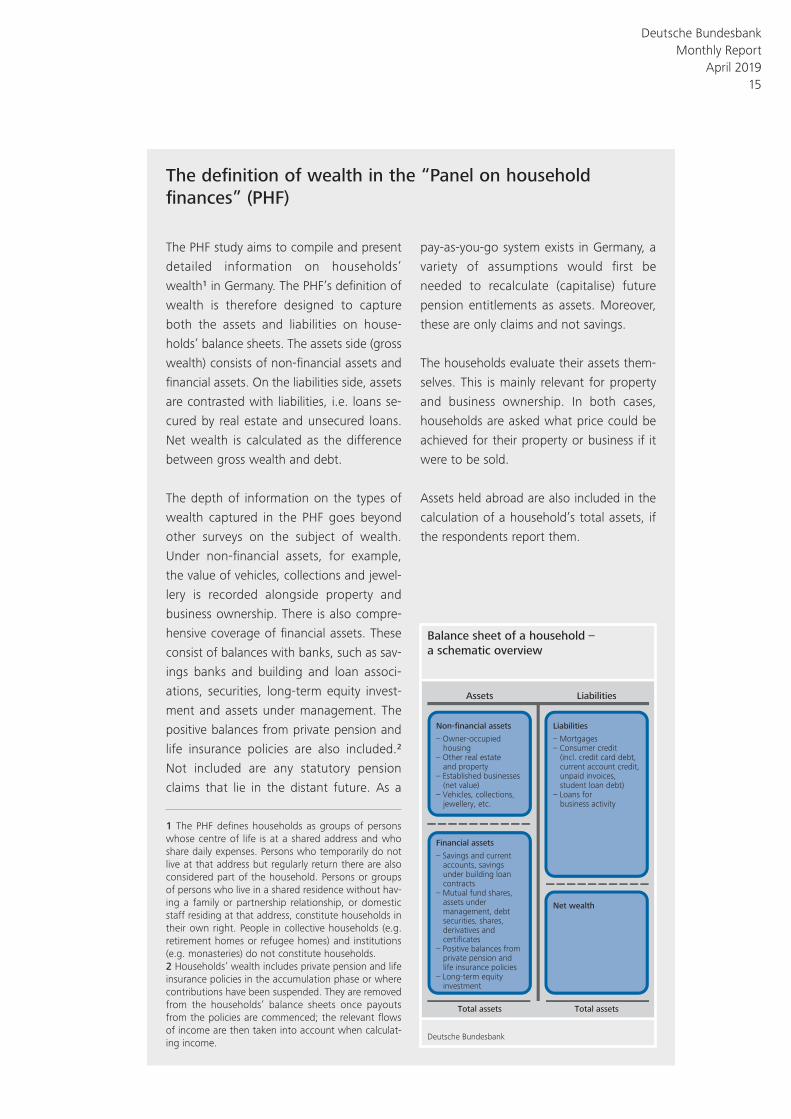
Balance sheet of a household –

a schematic overview

Deutsche Bundesbank

Net wealth

Liabilities

– Mortgages

– Consumer credit

(incl. credit card debt,

current account credit,

unpaid invoices,

student loan debt)

– Loans for

business activity

Non-financial assets

– Owner-occupied

housing

– Other real estate

and property

– Established businesses

(net value)

– Vehicles, collections,

jewellery, etc.

Financial assets

– Savings and current

accounts, savings

under building loan

contracts

– Mutual fund shares,

assets under

management, debt

securities, shares,

derivatives and

certificates

– Positive balances from

private pension and

life insurance policies

– Long-term equity

investment

LiabilitiesAssets

Total assetsTotal assets

1 The PHF defi nes households as groups of persons whose centre of life is at a shared address and who share daily expenses. Persons who temporarily do not live at that address but regularly return there are also considered part of the household. Persons or groups of persons who live in a shared residence without hav-ing a family or partnership relationship, or domestic staff residing at that address, constitute households in their own right. People in collective households (e.g. retirement homes or refugee homes) and institutions (e.g. monasteries) do not constitute households.2 Households’ wealth includes private pension and life insurance policies in the accumulation phase or where contributions have been suspended. They are removed from the households’ balance sheets once payouts from the policies are commenced; the relevant fl ows of income are then taken into account when calculat-ing income.


April 2019 15

persistently uneven distribution of wealth,

standing at 74% in 2017.5

Over the past few years, the academic litera-

ture describing income and wealth distribution

has increasingly looked at (very) wealthy house-

holds’ share of total wealth.6 On this basis, just

how uneven the distribution is can also be de-

duced from the share of wealth held by the top

10% in the net wealth distribution. In 2017, this

group possessed around 55% of total net

wealth in Germany.7 Values for a comparable

period are currently only available for the

United States, Italy and Austria. In 2016,

roughly 44% and 77% of total net wealth be-

longed to this group in Italy and the United

States respectively, whereas the figure for Aus-

tria stood at 56% in 2017. It amounted to 51%

for the euro area as a whole in 2014.8

Alongside the overall measures of the distribu-

tion of net wealth, the distribution of wealth

amongst individual groups of households, such

as those who own real estate, is also of inter-

est.9

Real estate ownership is a good indicator for a

household’s level of wealth. Households living

in a property they own have considerably

higher net wealth than tenant households.10

The median net wealth of owner households

amounted to €277,000 in 2017. For tenant

households, conversely, the median value is

only around €10,400. Similar structures can be

found in other countries both throughout Eur-

ope and worldwide. The highlighted differ-

ences are not only the result of whether a

household owns real estate or not, but are also

at least partly due to the differing household

structures of owners and tenants, for example

with regard to age, household size, marital sta-

tus of household members, and income.11 In

addition, rising real estate prices in the last few

years have had a significant impact on the

development of property- owning households’

wealth.

The well- documented differences between

eastern and western Germany with regard to

income and other economic indicators12 are

also apparent when examining wealth. The

median household in eastern Germany had

wealth of €23,400 in 2017; the median house-

hold in western Germany, by contrast, had

approximately four times as much wealth, at

€92,500. The lower proportion of home

owners in the eastern states presumably plays a

role here. The distribution of wealth as meas-

ured by the Gini coefficient is still somewhat

more uneven in the eastern states (77%) than

in the western states (72%).

Differences can also be identified in terms of

socio- demographic characteristics. The PHF

study captures a household’s wealth as a whole

rather than recording that of the individual

members of that household. The size and com-

position of a household are therefore signifi-

cant when determining the average and me-

dian wealth of certain household groups. At

€141,800, the average net wealth of single

person households in 2017 amounted to

slightly less than half of that of couple house-

Wealthiest 10% possess 55% of net wealth

Real estate own-ership indicates high net wealth

Marked differ-ences between eastern and western Germany

Single parents possess little wealth

5 The latest available Gini coefficient for the euro area dates back to the year 2014, when it amounted to 68.5%. 2014 figures for individual euro area countries can be found in Household Finance and Consumption Network (2016a).6 See Piketty (2014); and Saez and Zucman (2016).7 The share of wealth attributable to the top 10% of the distribution is probably underestimated (see Vermeulen (2018)). The approach behind the study “Panel on house-hold finances (PHF)” is to over- represent the wealthy households in the (unweighted) sample (see the box on p. 17). This goal has generally been achieved. However, as in all other comparable surveys, very wealthy households are missing from the PHF. None of the households sur-veyed in the PHF have assets amounting to €100 million or more. This under- recording is not offset through the weighting of the data.8 For Italy, see Banca d’Italia (2018); for the United States, Federal Reserve Bank (2017); for Austria, Oesterreichische Nationalbank (2019); for the euro area, Household Finance and Consumption Network (2016b).9 Only a few methods of breaking down households into different groups can be outlined here. Further breakdowns can be found in the tables on pp. 30 ff.10 In Germany, only 44% of households own their main residence. Of all the other euro area countries, only Austria has a similarly low share (46% in 2017). By way of compari-son, home ownership levels in Italy and Spain stood at around 70% and 80% respectively in 2014.11 See also p. 18.12 See Brenke (2014).


PHF study 2017: methodological design of the third survey

Between March and October 2017, 4,942

households comprising 9,710 persons aged

16 and over participated in the PHF study in

Germany. Some of the households (3,335)

took part in a PHF survey for the second or

third time. For the remaining 1,607 house-

holds, it was their fi rst survey. There was a

response rate of 33% for successfully con-

tacted households. The response rate was

around 70% for households that had al-

ready participated in the survey (panel

households) and only 16% for those ap-

proached for the fi rst time. The response

rate for the panel households is comparable

to other surveys conducted in Germany, but

the fi gure for households included in the

study for the fi rst time is relatively low,

which to some extent is likely due to the

general decline in willingness to participate

in surveys.

The methodology used in the third PHF sur-

vey in 2017 is largely based on that of the

previous surveys in 2010/ 2011 and 2014. As

before, computer- assisted personal inter-

views (CAPI) were carried out face- to- face

at the interviewee’s home. The just under

300 trained interviewers required a little

over an hour on average to complete an

interview.

In 2017, the target population again also

included households with at least one per-

son over 18, but did not include people liv-

ing in collective households (e.g. retirement

homes, student halls of residence and refu-

gee homes) or institutions (e.g. monasteries

or prisons).

Addresses of households approached for

the fi rst time were selected randomly from

lists provided by residence registration of-

fi ces. An oversampling feature was imple-

mented at this point, which means that

wealthy households are overrepresented in

the sample chosen.1 The higher selection

probability was taken into account in the

weighting, so that the results shown can be

regarded as being representative for house-

holds in Germany.

In order to ensure comparability across the

individual surveys, only minor modifi cations

were made to the PHF questionnaire for the

third wave. The questionnaire was ex-

panded in some areas to include questions

on households’ expectations regarding

house prices, for example.

Further information on the methodology

and background of the PHF survey can be

found at https:// www.bundesbank.de/ en/

bundesbank/ research/ panel- on- household-

finances.

1 Income tax statistics are used in sampling to divide smaller municipalities with less than 100,000 residents into “rich municipalities” and “other municipalities”. In cities with 100,000 residents and more, wealthy street sections are identifi ed using micro- geographic infor-mation on residential area and purchasing power. Fi-nally, the proportion of households in the sample is selected such that households in wealthy municipal-ities and wealthy street sections are oversampled com-pared with their numbers in the population.


April 2019 17

https://www.bundesbank.de/en/bundesbank/research/panel-on-household-finances

holds (€319,000). By contrast, the median

value for couple households is almost seven

times higher than that of people living alone.

As has also become evident in recent years,

single- parent households, in particular, have lit-

tle wealth. In 2017, half of these households

possessed less than €5,200 gross or €3,900 net

wealth.

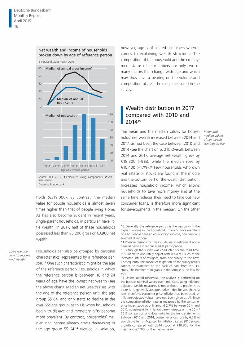
Households can also be grouped by personal

characteristics, represented by a reference per-

son.13 One such characteristic might be the age

of the reference person. Households in which

the reference person is between 16 and 24

years of age have the lowest net wealth (see

the above chart). Median net wealth rises with

the age of the reference person until the age

group 55-64, and only starts to decline in the

over-65s age group, as this is when households

begin to dissave and monetary gifts become

more prevalent. By contrast, households’ me-

dian net income already starts decreasing in

the age group 55-64.14 Viewed in isolation,

however, age is of limited usefulness when it

comes to explaining wealth structures. The

composition of the household and the employ-

ment status of its members are only two of

many factors that change with age and which

may thus have a bearing on the volume and

composition of asset holdings measured in the

survey.

Wealth distribution in 2017 compared with 2010 and 201415

The mean and the median values for house-

holds’ net wealth increased between 2014 and

2017, as had been the case between 2010 and

2014 (see the chart on p. 21). Overall, between

2014 and 2017, average net wealth grew by

€18,300 (+9%), while the median rose by

€10,400 (+17%).16 Few households who own

real estate or stocks are found in the middle

and the bottom part of the wealth distribution.

Increased household income, which allows

households to save more money and at the

same time reduces their need to take out new

consumer loans, is therefore more significant

for developments in the median. On the other

Life- cycle pat-tern for income and wealth

Mean and median values of net wealth continue to rise

Net wealth and income of households

broken down by age of reference person

Source: PHF 2017. 1 Calculated using components. 2 Self-

assessment.

Deutsche Bundesbank

10

20

30

40

50

60

0

30

60

90

120

150

180Median of net wealth

75 +

Median of annualnet income 2

65–7455–6445–5435–4425–3416–24

Age of reference person

€ thousand, as at March 2019

Median of annual gross income1

13 Generally, the reference person is the person with the highest income in the household. If two or more members of a household have an equally high income, one person is selected at random.14 Possible reasons for this include (early) retirement and a general decline in labour market participation.15 Although the survey was conducted for the third time, it is unable to accurately depict certain events, such as the increased influx of refugees, from one survey to the next. Consequently, the impact of migration on the survey results cannot be examined on the basis of data from the PHF study. The number of migrants in the sample is too low for this.16 Unless stated otherwise, the analysis is performed on the basis of nominal values over time. Calculating inflation- adjusted wealth measures is not without its problems as there is no generally accepted price index for wealth. As a rule, therefore, consumer price inflation has been used, or inflation- adjusted values have not been given at all. Since the cumulative inflation rate as measured by the consumer price index stood at only around 2.7% between 2014 and 2017, adjustment for inflation barely impacts on the 2014/ 2017 comparison and does not alter the trend statements. Between 2010 and 2014, consumer prices rose by 6.7% in cumulative terms. Adjusted for inflation, i.e. at 2010 prices, growth compared with 2014 stood at €10,800 for the mean and €7,700 for the median value.


Selected research results based on PHF data

The study “Panel on household fi nances” (PHF) not only provides important results for advising policy makers, it is also used for aca-demic research on the behaviour and fi nancial situation of German households. More than 200 researchers in Germany and abroad are now using the anonymised data for research projects. The empirical and theoretical pro-jects cover a large range of subjects.

In recent years, central banks around the world have dropped their policy rates to his-torical lows and pursued non- standard policy measures such as extensive programmes to purchase government bonds. Drawing on micro data from the PHF and similar house-hold surveys by other central banks, a number of current research projects are addressing the question regarding the extent to which mon-etary policy infl uences the distribution of households’ wealth and income in Germany and other European countries.1

Tzamourani (2019) analyses the unhedged interest rate exposure2 of households in the euro area. This indicator captures the extent to which households respond to changes in real interest rates and refl ects the direct gains and losses in their net interest income after such changes. On the whole, households in individual countries are exposed to very differ-ent types of interest rate risk. These national differences are mainly caused by the hetero-geneous distribution of adjustable- rate mort-gages. In countries where the prevalence of adjustable- rate mortgages issued is high, households’ interest rate exposure is negative on average, i.e. where infl ation is constant, households would be impacted negatively on average by an interest rate hike. In Germany and other countries where the number of people with adjustable- rate mortgages is low, households would initially benefi t on average from a hike in interest rates (where infl ation remains constant).

Given the importance of housing wealth to the distribution of wealth within individual

countries and across euro area countries, the differences in the investment behaviour of owner households and tenant households have been the focus of a number of ongoing research projects. Le Blanc and Schmidt (2019a) investigate differences in owners’ and tenants’ savings behaviour, noting that house-holds do not cut back on their active savings fl ows despite passive saving in the form of mortgage repayments, but rather save on top of their pre- existing contracts.

While this article focuses on the distribution of wealth, the fi nancial situation of house-holds is multidimensional and characterised by the joint distribution of consumption, in-come and wealth.3 In an ongoing research project, Le Blanc and Schmidt (2019b) esti-mate the joint distribution of consumption, income and wealth in Germany. One provi-sional result of this project is that consump-tion and income are more evenly distributed than net wealth.

Inherited assets also play a major role in wealth distribution and inequality. Pasteau and Zhu (2018) analyse inherited wealth as an additional potential factor in explaining the choice of partner. One of the main fi ndings of their analysis is that prospects of an inherit-ance are more than twice as important than income in explaining marriage choice. As the number of inheritances is expected to rise in the coming years, this will also have implica-tions on the dynamics of wealth inequality.

In addition to the detailed information on the components of wealth, the PHF also provides information on households’ expectations, which are crucial to consumption and invest-ment behaviour.

1 See Deutsche Bundesbank (2016a); Casiraghi et al. (2016); Ampudia et al. (2018); Lenza and Slacalek (2019).2 Auclert (2019) defi nes unhedged interest rate expos-ure as the difference between maturing assets and liabil ities.3 See Fisher et al. (2018).


April 2019 19

hand, increases in real estate and share prices

are likely to have played a key role in the rise in

net wealth in the upper range of the distribu-

tion, where real estate and share ownership

are widespread.

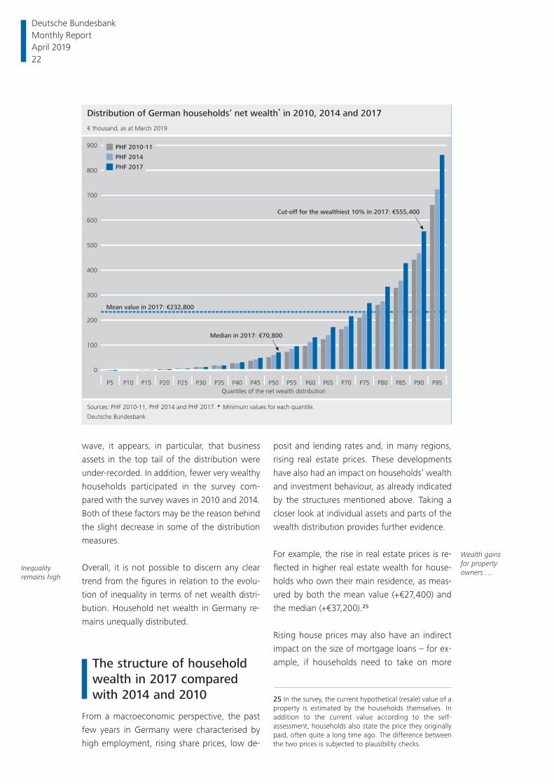
The values breaking down net wealth distribu-

tion17 into ten equal parts increased across the

board. While the cut- offs for the bottom four

deciles were lower in 2014 than in 2010, they

rebounded to 2010 levels in 2017.18 In absolute

terms, however, these increases are small and

amounted to between €100 and €4,200 in

these deciles. Measured in euro terms, upward

shifts in the top part of the wealth distribution

are greater, as expected. In order to rank

among the wealthiest 10% of households in

Germany, around €442,000 was needed in

2010, roughly €468,000 in 2014 and just over

€555,400 in 2017.19 However, even relative to

the figure determined in the preceding study,

the percentage increases in the upper half of

the distribution were more pronounced than in

the lower half of the distribution.

The major significance of real estate in terms of

household wealth and its distribution was al-

ready apparent in the first two waves of the

PHF study.20 It is therefore hardly surprising that

wealth has risen especially sharply, in both ab-

solute terms and relative to the values for 2014,

for those deciles of the net wealth distribution

in which property- owning households are es-

pecially common, i.e. the wealthiest 40% of

households.21

Broad- based increase in net wealth

Goldfayn- Frank and Wohlfart (2018) analyse the infl ation expectations of households in eastern and western Germany. They docu-ment the fact that the infl ation expectations of households that were located in East Ger-many before German reunifi cation are one percentage point higher than the infl ation ex-pectations of western German households. The authors cite the surprisingly high infl ation that eastern German households experienced after 1989 as a reason for their signifi cantly higher infl ation expectations. The differing in-fl ation expectations are still seen today in the investment behaviour of people born in east-ern Germany.

In an ongoing research project, Kindermann et al. (2019) studied the expectations of households regarding the development of house prices over the following twelve months. Two clear patterns can be identifi ed when it comes to households that provide in-formation on how house prices will evolve in their area in the following twelve months.

First, households tend to underestimate future house price developments.4 Second, a differ-ence emerges between tenant households and owner households. Tenants expect higher infl ation than owner households, especially those that intend to purchase property.

Interested researchers may apply for access to the PHF’s anonymised data (scientifi c use fi les) for academic projects. More information and forms to apply for access to the data can be downloaded from the Bundesbank’s website at www.bundesbank.de/ phf- data.

4 These results cannot be generalised, however, as the underlying data only recognise the upturn in house prices.

17 The discussion in this article focuses on net wealth dis-tribution. Corresponding analyses of gross wealth distribu-tion can be carried out using the tables in the annex on pp. 30 ff.18 These figures provide only limited information on changes in individual households’ net wealth, as house-holds’ position in the distribution may change.19 At 2010 prices, the values are €436,600 for 2014 and €503,500 for 2017.20 See Deutsche Bundesbank (2013) and Deutsche Bun-desbank (2016b).21 In these parts of the net wealth distribution, more than 60% of households own real estate.


www.bundesbank.de/phf-data

As a result of these developments, indicators

focusing on the range between certain parts of

the wealth distribution have risen since 2010.

For example, the difference between the top

and bottom quartiles of the net wealth distri-

bution (“interquartile range”) increased from

around €203,000 to €262,000. This corres-

ponds to growth of almost 30% between 2010

and 2017.22

Looking at the gaps between the deciles of the

distribution and the median as the midpoint of

the distribution, it is striking that both the top

and bottom deciles have moved further away

from the median. The gap between the median

and the first decile is now around €19,400

greater than it was in 2010. The gap between

the ninth decile and the median rose by around

€93,600 compared with 2010. The part of the

distribution with a high proportion of property

owners (see the chart on p. 23), in particular,

became further removed from the median in

relative terms between 2010 and 2017. This de-

velopment also reflects the fact that the per-

centage of households in Germany who are

homeowners is below 50%. In other words,

the median household does not own its own

home and is therefore not benefiting from the

rise in real estate prices.

The widening gaps between individual parts of

the net wealth distribution tend to point to-

wards an increase in inequality. By contrast,

other indicators measuring inequality in the dis-

tribution of household net wealth, which are

listed in the table on page 23, fell slightly over

time or remained unchanged.

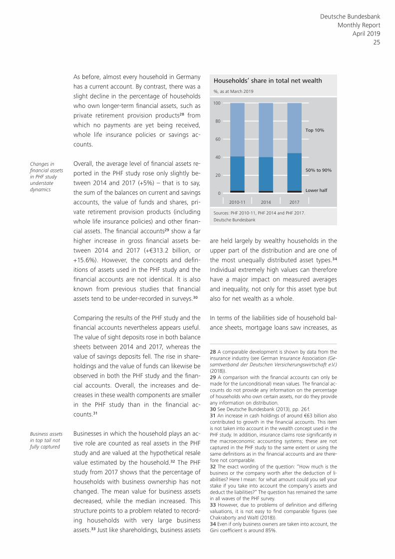
The Gini coefficient and the share of total net

wealth held by the wealthiest 10% of house-

holds decreased by 2 and 5 percentage points

respectively. The ratio of the mean to the me-

dian and the gap between the wealthiest 10%

of households and the median changed only

slightly. As before, the lower half of the distri-

bution of wealth accounts for around 3% of

total net wealth (see the chart on p. 25). The

share of total wealth held by the top 10% of

households fell from about 60% in 2014 to

55% in 2017. In return, the share held by the

group between the 90th percentile and the

median rose from 38% to 42% over the same

period.

Similar, smaller changes in these indicators

were revealed in the past in other wealth sur-

veys for Germany and other countries without

resulting in a revised assessment of inequality.23

The declines in the Gini coefficient and the

share of total net wealth held by the top 10%

of households should not be overstated, in part

due to the known issues related to recording

wealth in the top tail.24 In the 2017 survey

Increase in absolute gap between distri-bution tails and median

Real estate important for wealth dynam-ics in upper part of wealth distribution

Slight fall in standard indica-tors for measur-ing inequality

Under- recording of wealth in top tail affects measures of inequality

Mean and median values of German

households’ net wealth distribution

Sources: PHF 2010-11, PHF 2014, PHF 2017.

Deutsche Bundesbank

0

50

100

150

200

250


Mean Median

20172017 2010-112010-11 20142014

22 The interquartile range is a measure of statistical disper-sion. When interpreting the data, it is important to note that the interquartile range would increase even if the wealth of all households rose by the same factor. At 2010 prices, the interquartile range was around €237,200 in 2017 (+17% compared with 2010).23 In Italy, the Gini coefficient for net wealth has hovered between 60% and 64% since the mid-1990s (Banca d’Italia (2018)), whilst in Austria it has fluctuated between 76% and 73% since 2010 (Oesterreichische Nationalbank (2019)). For Germany, too, data from the Socio- Economic Panel (SOEP) and the sample survey of income and expend-iture (EVS) show that the Gini coefficient has, in the past, tended to fluctuate slightly by between 1 and 2 percentage points (see Deutsche Bundesbank (2016a), pp. 18-20 and the chart on p. 17; and Grabka and Westermeier (2014)).24 See Vermeulen (2016); Grabka and Westermeier (2014); Deutsche Bundesbank (2013); and Chakraborty and Waltl (2018).


April 2019 21

wave, it appears, in particular, that business

assets in the top tail of the distribution were

under- recorded. In addition, fewer very wealthy

households participated in the survey com-

pared with the survey waves in 2010 and 2014.

Both of these factors may be the reason behind

the slight decrease in some of the distribution

measures.

Overall, it is not possible to discern any clear

trend from the figures in relation to the evolu-

tion of inequality in terms of net wealth distri-

bution. Household net wealth in Germany re-

mains unequally distributed.

The structure of household wealth in 2017 compared with 2014 and 2010

From a macroeconomic perspective, the past

few years in Germany were characterised by

high employment, rising share prices, low de-

posit and lending rates and, in many regions,

rising real estate prices. These developments

have also had an impact on households’ wealth

and investment behaviour, as already indicated

by the structures mentioned above. Taking a

closer look at individual assets and parts of the

wealth distribution provides further evidence.

For example, the rise in real estate prices is re-

flected in higher real estate wealth for house-

holds who own their main residence, as meas-

ured by both the mean value (+€27,400) and

the median (+€37,200).25

Rising house prices may also have an indirect

impact on the size of mortgage loans – for ex-

ample, if households need to take on more

Inequality remains high

Wealth gains for property owners …

Distribution of German households’ net wealth* in 2010, 2014 and 2017

Sources: PHF 2010-11, PHF 2014 and PHF 2017. * Minimum values for each quantile.

Deutsche Bundesbank

0

100

200

300

400

500

600

700

800

900

P95P90P85P80P75P70P65P60P55P50P45P40P35P30P25P20P15P10P5

Quantiles of the net wealth distribution

PHF 2010-11

PHF 2014

PHF 2017

Mean value in 2017: €232,800

Cut-off for the wealthiest 10% in 2017: €555,400

Median in 2017: €70,800


25 In the survey, the current hypothetical (resale) value of a property is estimated by the households themselves. In addition to the current value according to the self- assessment, households also state the price they originally paid, often quite a long time ago. The difference between the two prices is subjected to plausibility checks.


debt in order to be able to afford a property, or

if properties are more heavily leveraged in view

of low lending rates. Median mortgage debt

was €81,000 in 2017, compared with €76,400

in 2014. Not only has median mortgage debt

increased, the mean value of outstanding mort-

gage debt for households with mortgage debt

also rose by around €14,000.26 However, this

debt is backed by real estate assets that have

appreciated even more. The, relatively speak-

ing, largest increases in mortgage debt were

recorded by the wealthiest 10% of households

in terms of net wealth.27 The unconditional

mean value for mortgage debt rose by around

€28,700 in this part of the distribution. These

households usually have sufficient financial re-

sources to meet the capital requirements for a

mortgage loan. As described in the section

below entitled “Households’ debt situation”,

debt service as a share of income has declined

for indebted households as a whole.

Changes in holdings of shares and funds reflect

the rise in share prices between 2014 and 2017.

On average, the value of shares for those

households with direct shareholdings rose by

around €5,000, or 13%; by contrast, the me-

dian remained virtually unchanged at just under

€10,000. The German stock market index in-

creased by almost 30% between mid- April

2014 and mid- April 2017. As a result, the in-

crease measured in the PHF study is lower.

However, the data do not allow for a separate

analysis of the changes in the value of possible

acquisitions and sales. Furthermore, changes in

the composition of the shareholders cannot be

taken into account. If, for example, households

with large share portfolios sell part of them and

other households invest smaller amounts in the

equity market, this can affect the mean value

as well as the median, despite the fact that the

percentage of households with shareholdings

does not change. This could also be a reason

for the lower values for fund holdings.

In terms of financial assets, the increase in

assets on current accounts is striking. Com-

pared with 2014, the average current account

balance increased by 65%, with the median ris-

ing to a similar extent. This development sug-

gests that households in Germany continue to

have a preference for liquid forms of invest-

ment that are perceived as low- risk.

… and house-holds with shareholdings

Fewer house-holds with longer- term financial assets

Real estate ownership along the net

wealth distribution

Source: PHF 2017. 1 In this context, ownership of other prop-erties includes only those properties which are not used for business purposes.

Deutsche Bundesbank

1 2 3 4 5 6 7 8 9 10

0

20

40

60

80

100

Share of households as a percentage, as at March 2019

Deciles of the net wealth distribution

Share of households with ownership of main residence

Share of householdswith ownership of other properties1

Indicators of net wealth distribution in 2010-11, 2014 and 2017

Item 2010-11 2014 2017

Interquartile range €203,000 €221,000 €262,000P90- P10 €442,000 €468,000 €555,000

Mean value/ median 3.8 3.6 3.3P90/ P50 8.6 7.8 7.8

Gini coeffi cient 76% 76% 74%

Share of total net wealth held by wealthiest 10% 59% 60% 55%

Source: PHF 2017 – data as at March 2019.

Deutsche Bundesbank

26 When interpreting these figures, it should be borne in mind that reference is made to the current outstanding loan amount, and that loans taken out some time ago and new loans are therefore analysed together.27 For this group of very wealthy households, the share of households who own property in addition to their main residence rose by 5 percentage points. Part of the growth in mortgage lending is therefore probably attributable to new builds or purchases of additional properties.


April 2019 23

Self-assessment of position in the distribution of wealth

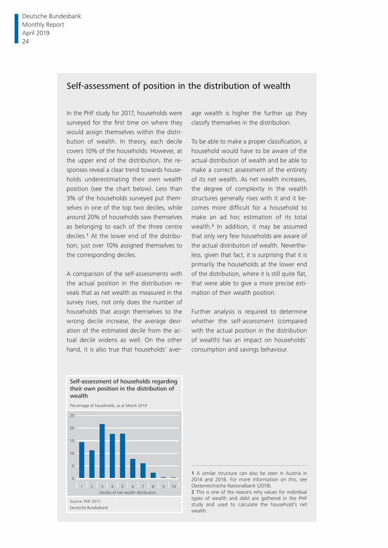
In the PHF study for 2017, households were

surveyed for the fi rst time on where they

would assign themselves within the distri-

bution of wealth. In theory, each decile

covers 10% of the households. However, at

the upper end of the distribution, the re-

sponses reveal a clear trend towards house-

holds underestimating their own wealth

position (see the chart below). Less than

3% of the households surveyed put them-

selves in one of the top two deciles, while

around 20% of households saw themselves

as belonging to each of the three centre

deciles.1 At the lower end of the distribu-

tion, just over 10% assigned themselves to

the corresponding deciles.

A comparison of the self- assessments with

the actual position in the distribution re-

veals that as net wealth as measured in the

survey rises, not only does the number of

households that assign themselves to the

wrong decile increase, the average devi-

ation of the estimated decile from the ac-

tual decile widens as well. On the other

hand, it is also true that households’ aver-

age wealth is higher the further up they

classify themselves in the distribution.

To be able to make a proper classifi cation, a

household would have to be aware of the

actual distribution of wealth and be able to

make a correct assessment of the entirety

of its net wealth. As net wealth increases,

the degree of complexity in the wealth

structures generally rises with it and it be-

comes more diffi cult for a household to

make an ad hoc estimation of its total

wealth.2 In addition, it may be assumed

that only very few households are aware of

the actual distribution of wealth. Neverthe-

less, given that fact, it is surprising that it is

primarily the households at the lower end

of the distribution, where it is still quite fl at,

that were able to give a more precise esti-

mation of their wealth position.

Further analysis is required to determine

whether the self- assessment (compared

with the actual position in the distribution

of wealth) has an impact on households’

consumption and savings behaviour.

1 A similar structure can also be seen in Austria in 2014 and 2016. For more information on this, see Oesterreichische Nationalbank (2019).2 This is one of the reasons why values for individual types of wealth and debt are gathered in the PHF study and used to calculate the household’s net wealth.

Self-assessment of households regarding

their own position in the distribution of

wealth

Source: PHF 2017.

Deutsche Bundesbank

0

5

10

15

20

25

Percentage of households, as at March 2019

10987654321

Deciles of net wealth distribution


As before, almost every household in Germany

has a current account. By contrast, there was a

slight decline in the percentage of households

who own longer- term financial assets, such as

private retirement provision products28 from

which no payments are yet being received,

whole life insurance policies or savings ac-

counts.

Overall, the average level of financial assets re-

ported in the PHF study rose only slightly be-

tween 2014 and 2017 (+5%) – that is to say,

the sum of the balances on current and savings

accounts, the value of funds and shares, pri-

vate retirement provision products (including

whole life insurance policies) and other finan-

cial assets. The financial accounts29 show a far

higher increase in gross financial assets be-

tween 2014 and 2017 (+€313.2 billion, or

+15.6%). However, the concepts and defin-

itions of assets used in the PHF study and the

financial accounts are not identical. It is also

known from previous studies that financial

assets tend to be under- recorded in surveys.30

Comparing the results of the PHF study and the

financial accounts nevertheless appears useful.

The value of sight deposits rose in both balance

sheets between 2014 and 2017, whereas the

value of savings deposits fell. The rise in share-

holdings and the value of funds can likewise be

observed in both the PHF study and the finan-

cial accounts. Overall, the increases and de-

creases in these wealth components are smaller

in the PHF study than in the financial ac-

counts.31

Businesses in which the household plays an ac-

tive role are counted as real assets in the PHF

study and are valued at the hypothetical resale

value estimated by the household.32 The PHF

study from 2017 shows that the percentage of

households with business ownership has not

changed. The mean value for business assets

decreased, while the median increased. This

structure points to a problem related to record-

ing households with very large business

assets.33 Just like shareholdings, business assets

are held largely by wealthy households in the

upper part of the distribution and are one of

the most unequally distributed asset types.34

Individual extremely high values can therefore

have a major impact on measured averages

and inequality, not only for this asset type but

also for net wealth as a whole.

In terms of the liabilities side of household bal-

ance sheets, mortgage loans saw increases, as

Changes in financial assets in PHF study understate dynamics

Business assets in top tail not fully captured

Households’ share in total net wealth

Sources: PHF 2010-11, PHF 2014 and PHF 2017.

Deutsche Bundesbank

0

20

40

60

80

100

%, as at March 2019

201720142010-11

50% to 90%

Top 10%

Lower half

28 A comparable development is shown by data from the insurance industry (see German Insurance Association (Ge-samtverband der Deutschen Versicherungswirtschaft e.V.) (2018)).29 A comparison with the financial accounts can only be made for the (unconditional) mean values. The financial ac-counts do not provide any information on the percentage of households who own certain assets, nor do they provide any information on distribution.30 See Deutsche Bundesbank (2013), pp. 26 f.31 An increase in cash holdings of around €63 billion also contributed to growth in the financial accounts. This item is not taken into account in the wealth concept used in the PHF study. In addition, insurance claims rose significantly in the macroeconomic accounting systems; these are not captured in the PHF study to the same extent or using the same definitions as in the financial accounts and are there-fore not comparable.32 The exact wording of the question: “How much is the business or the company worth after the deduction of li-abilities? Here I mean: for what amount could you sell your stake if you take into account the company’s assets and deduct the liabilities?” The question has remained the same in all waves of the PHF survey.33 However, due to problems of definition and differing valuations, it is not easy to find comparable figures (see Chakraborty and Waltl (2018)).34 Even if only business owners are taken into account, the Gini coefficient is around 85%.


April 2019 25

discussed above. The outstanding amount of

unsecured loans also rose in 2017, with the me-

dian now standing at €4,900, compared with

€3,500 in 2014 and €3,200 in 2010. The per-

centage of households with unsecured loans

remained stable between 2014 and 2017 at

33%, however. On a related note, the share of

households with negative net wealth, i.e.

households whose debt exceeds their assets,

fell slightly from 8.7% in 2014 to 7.5% in

2017.35

The structure of portfolios along the net wealth

distribution barely changed between 2010 and

2017. Whilst, in the upper range of the distribu-

tion, real assets and real estate make up the

bulk of wealth, in the lower half of the distribu-

tion households’ wealth consists almost exclu-

sively of financial assets (see the chart on

p. 27). Levels of outstanding debt increase as

net wealth rises.

Saving and wealth

Upward and downward movements in particu-

lar asset prices are not the only factors that

may alter the structure of asset holdings de-

scribed above; it is also shaped, in part, by

households’ saving and investment behaviour.

While changes in saving and investment pat-

terns generally only start having an impact on

wealth composition over the long run, they are

nevertheless relevant when it comes to the ef-

fect of monetary policy measures.

Looking at 2016, analyses on the basis of a

special survey conducted as part of the PHF

study show that households modify their sav-

ings behaviour in response to low interest rates

to a certain extent.36 There appears to be a ten-

Amounts out-standing on loans rising

Composition of wealth along wealth distribu-tion unchanged

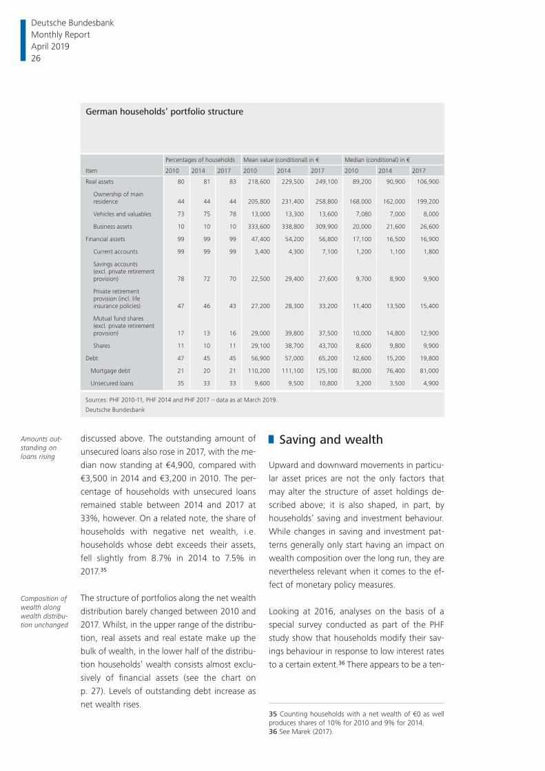
German households’ portfolio structure

Item

Percentages of households Mean value (conditional) in € Median (conditional) in €

2010 2014 2017 2010 2014 2017 2010 2014 2017

Real assets 80 81 83 218,600 229,500 249,100 89,200 90,900 106,900

Ownership of main residence 44 44 44 205,800 231,400 258,800 168,000 162,000 199,200

Vehicles and valuables 73 75 78 13,000 13,300 13,600 7,080 7,000 8,000

Business assets 10 10 10 333,600 338,800 309,900 20,000 21,600 26,600

Financial assets 99 99 99 47,400 54,200 56,800 17,100 16,500 16,900

Current accounts 99 99 99 3,400 4,300 7,100 1,200 1,100 1,800

Savings accounts(excl. private retirement provision) 78 72 70 22,500 29,400 27,600 9,700 8,900 9,900

Private retirement provision (incl. life insurance policies) 47 46 43 27,200 28,300 33,200 11,400 13,500 15,400

Mutual fund shares (excl. private retirement provision) 17 13 16 29,000 39,800 37,500 10,000 14,800 12,900

Shares 11 10 11 29,100 38,700 43,700 8,600 9,800 9,900

Debt 47 45 45 56,900 57,000 65,200 12,600 15,200 19,800

Mortgage debt 21 20 21 110,200 111,100 125,100 80,000 76,400 81,000

Unsecured loans 35 33 33 9,600 9,500 10,800 3,200 3,500 4,900

Sources: PHF 2010-11, PHF 2014 and PHF 2017 – data as at March 2019.

Deutsche Bundesbank

35 Counting households with a net wealth of €0 as well produces shares of 10% for 2010 and 9% for 2014.36 See Marek (2017).


dency towards both reduced saving efforts and

an adjustment in terms of saving objectives.

Measured in terms of the share of households

who claim to regularly save, the data collected

in 2017 show no evidence of a decline in sav-

ing efforts. Around 63% of the households re-

port that they put aside a set amount of money

every month, meaning there has even been a

4 percentage point rise in that share since

2014. At the same time, the proportion of

households who say they are unable to save

because they lack the financial means has fallen

by 4 percentage points. The favourable condi-

tions on the labour market are likely to be a

factor in this.

Over the three waves, the PHF study also pro-

vides insights into why households save. Mo-

tives for saving have evidently changed over

time. The proportion of households citing buy-

ing property as their main motive for saving

grew between 2010 and 2017. An increase was

apparent between 2010 and 2014 especially

among younger households, for whom this

motive is traditionally particularly important

(see the chart on p. 28), while a slight fall in the

share can be seen between 2014 and 2017.

Over the last three years, the share of house-

holds for whom renovating, refurbishing or ex-

tending a property is the main reason for sav-

ing has also increased,37 with around 9% citing

it as their most important motivation in 2017.

Rising property prices seem to be acting as in-

centives to invest in maintaining and upgrading

real estate. Low interest rates are also making it

possible for borrowers to obtain loans for reno-

vating an owner- occupied property at favour-

able conditions.

The proportion of households citing “retire-

ment provision” as their most important motive

for saving, meanwhile, has dropped from 22%

in 2010 to 17% in 2017. This decline is consist-

ent with the reduced share of households pos-

sessing long- term savings deposits and con-

tracts for private retirement provision described

above. The waning significance of this motive

for saving was already apparent between 2010

and 2014 and can be seen across all age

groups, but is particularly pronounced among

the older households over 65 years of age. For

that group, saving is increasingly motivated by

supporting children and grandchildren and by

legacy and gifting purposes.

Households’ debt situation

The primary focus of this article so far has been

households’ wealth and how that wealth is

structured. For central banks, however, it is not

just households’ investment behaviour that is

of interest but also the decisions households

make when it comes to borrowing. The house-

hold debt situation can be ascertained by refer-

More than half of households save on a regular basis

Motives for saving changing

Fewer house-holds saving with retirement provision in mind

Breakdown of households’ wealth

by size*

Source: PHF 2017. * Mean values (unconditional).

Deutsche Bundesbank

200

0

200

400

600

800

1,000

1,200

1,400

–

+

+

+

+

+

+

+

Assets and/or debt in € thousand, as at March 2019

Quantiles of the net wealth distribution

90 –

100

80 –

90

60 –

80

40 –

60

20 –

40

0 –

20

Total

Financial assets

Real estate

Real assets excl. real estate

Unsecured loans

Mortgage debt

37 The year 2014 was the first time participants were asked about this particular motive for saving.


April 2019 27

ence to various indicators. These include, for

instance, the proportion of indebted house-

holds, the level of debt and measures of house-

holds’ debt sustainability.

According to the PHF study, there has been

barely any change in the share of indebted

households between 2010 and 2017: the per-

centage of households with some kind of out-

standing debt38 still stands at roughly 45%.

Very little has changed with respect to the

underlying structures, too. Fewer households

have mortgage loans than have unsecured

types of credit but, as is to be expected, the

amounts owed on mortgage loans are far

higher (median: €81,000) than outstanding

amounts for other loans (median: €4,900).

Both values are higher than in 2014; in particu-

lar, the outstanding amounts for unsecured

loans are still low.

More important than the absolute amount of

outstanding debt is debt sustainability, in other

words the interplay between income, indebt-

edness and debt service. The ratio of debt ser-

vice, i.e. interest and principal repayments, to

net income frequently figures in analyses re-

lated to issues of financial stability and in a

monetary policy context.39

Moving up the income scale, both the share of

households with outstanding debt and the

amount owed by this group of households

rises. Out of the households with an annual net

income of up to around €13,200, roughly 32%

had debts outstanding in 2017; in the group of

households with an annual net income of over

€37,200, meanwhile, the figure was slightly

greater than 60%.

Interest and principal repayments as a share of

net income fell from an average of 23% to

20% between 2010 and 2017. As the chart on

page 29 shows, the top tail of the distribution

in particular saw changes compared with 2014.

From about the seventh decile, we start to see

a decrease. The ninth decile starts out at 37%

of net income in 2017; in 2010 that figure was

47% and in 2014 it stood at 42%. Households

with high interest and principal repayments in

2017 were thus also needing to use a smaller

portion of their income to cover them.

There are two factors which likely play a role in

this change: the increase in households’ net in-

come and the persistently low lending rates.

Looking at purely the interest element of debt

service as a proportion of income, there was a

very strong decrease of 4 percentage points

Share of indebted households unchanged

Share of indebted house-holds rises with income

Debt service as a share of net income lower

Interest burden as a share of income lower

Most important motive for saving

by age of reference person

%, as at March 2019

0 10 20 30 40 50 60 70 80 90 100

Sources: PHF 2010-11, PHF 2014, PHF 2017.

Deutsche Bundesbank

Over 65

45 to 65

Under 45

PHF 2010-11

PHF 2014

PHF 2017

PHF 2010-11

PHF 2014

PHF 2017

PHF 2010-11

PHF 2014

PHF 2017

Property purchase Property renovation

Consumer purchases Emergencies

Retirement provision Children/grandchildren

Other

38 In the context of the PHF study, this covers mortgage loans as well as unsecured loans including overdrawn cur-rent accounts and money owed to other households.39 See Deutsche Bundesbank (2019).


between 2010 and 2017 to an average of 6%

for indebted households. A significant part of

the reduction in debt service relative to net in-

come can thus be attributed to lower interest

payments for new loans or loans where the

fixed interest rate has expired.

Summary

The PHF study provides an overview of the fi-

nancial situation of households in Germany in

2017. It shows that both the average wealth of

households and the median increased signifi-

cantly between 2014 and 2017. Net wealth

rose particularly in those sections of the distri-

bution containing a high proportion of prop-

erty owners. The findings thus again highlight

the important role played by real estate in

households’ asset holdings.

Compared with the results for 2014 and 2010,

it is also evident that households in Germany

remain hesitant to invest in securities, and hold

a substantial portion of their wealth in liquid

forms of investment that are perceived as low

risk, despite the fact that these are currently

only yielding low returns. There are initial indi-

cations that fewer households are investing in

longer- term assets such as voluntary private

pension plans or whole life insurance policies.

When it comes to debt, households are bene-

fiting from low lending rates.

Measures of inequality exhibited only minor

changes between 2014 and 2017 and no clear

trend is discernible. While the standard indica-

tors used to measure inequality – such as the

Gini coefficient and the share of total net

wealth held by the wealthiest households – fell

slightly, the gap between the upper and lower

part of the distribution widened. Germany re-

mains a country in which wealth is distributed

unequally.

The PHF study testifies to the fact that wealth

distribution and the underlying portfolio struc-

tures of Germany’s households are changing

only slowly. Even against a backdrop of strong

asset price hikes, sustained low interest rates

and a healthy economy, there were no major

shifts so far as measured inequality and port-

folio structures were concerned.

Table appendix

Only a small selection of the figures on German

household finances could be presented in the

main article on the PHF survey findings. The fol-

lowing appendix contains further tables. Each

table shows the percentage of households

Distribution of debt service as a share of net income for indebted households*

Sources: PHF 2010-11, PHF 2014, PHF 2017. * The shares refer to indebted households paying off debt.

Deutsche Bundesbank

0

10

20

30

40

50

60

70

%, as at March 2019

P95P90P85P80P75P70P65P60P55P50P45P40P35P30P25P20P15P10P5

Quantiles: debt service as a share of net income

PHF 2010-11

PHF 2014

PHF 2017


April 2019 29

who own a particular asset or are in debt (par-

ticipation rates), the conditional mean value

and the conditional median. “Conditional” in

this context means that the mean values and

medians are all computed only for those house-

holds who possess a given asset or have a par-

ticular type of debt. Where no participation

rate is stated, it is 100% and the mean values

and medians refer to all households. The afore-

mentioned values are shown in total as well as

broken down by the age, nationality, labour

market status and education of the reference

person,40 the type of household, the region in

which a household lives and its homeowner-

ship status. In addition, the households are also

differentiated according to where they lie in

the distributions of net wealth and gross in-

come.

Participation rate, mean value and conditional distribution of gross and net wealth, fi nancial and real assets, debt and annual gross and net income

Figures in €

ItemGross wealth

Net wealth Debt

Real assets (gross)

Financial assets (gross)

Gross income ( annual)

Net income ( annual, self-assess-ment)

Participation rate in % 100 100 45 83 99 100 100

Mean value (conditional) 262,500 232,800 65,200 249,100 56,800 53,000 36,700

Conditional distribution 5th percentile 300 – 2,800 300 500 0 7,900 8,90010th percentile 1,100 100 600 1,400 300 12,200 11,90020th percentile 6,000 3,000 2,400 4,900 2,000 19,300 15,60030th percentile 15,500 11,800 5,600 10,900 4,900 26,300 19,80040th percentile 38,100 31,200 10,000 37,100 9,500 32,900 24,00050th percentile 86,400 70,800 19,800 106,900 16,900 40,100 27,60060th percentile 167,100 131,000 36,500 175,500 29,500 47,800 32,30070th percentile 260,000 215,400 63,500 249,900 49,000 58,700 38,20080th percentile 379,800 334,000 101,900 346,600 79,500 73,800 44,40090th percentile 621,000 555,400 174,100 540,300 147,000 100,600 59,60095th percentile 969,100 861,600 265,500 898,400 224,400 137,300 72,000

Deutsche Bundesbank

40 In this context, the reference person is always the per-son with the highest income in the household. If two or more members of a household have an equally high in-come, one person is selected at random.


Gross and net wealth and debt, in total and by household characteristics

Figures in €

Item

Gross wealth Net wealth Debt

Mean value Median

Mean value Median

Participa-tion rate in %

Condi-tional mean value

Condi-tional median

All households 262,500 86,400 232,800 70,800 45 65,200 19,800

Regioneast1 110,400 26,700 93,200 23,400 45 38,200 9,700west 302,500 123,300 269,600 92,500 45 72,300 24,700

of which: region 12 313,600 88,500 281,100 74,300 47 69,800 29,100region 23 349,000 165,900 314,000 139,800 42 82,500 28,700region 34 236,000 74,500 205,600 60,300 49 62,300 16,900

Homeowner statusOwner without mortgage 513,400 319,700 494,900 317,100 25 74,900 19,300Owner with mortgage 527,300 316,800 406,000 218,400 100 121,300 85,400Tenant 61,400 13,400 54,900 10,400 38 17,000 5,000

Type of householdSingle household 156,500 27,400 141,800 22,200 33 44,200 10,000Single-parent household 80,300 5,200 58,000 3,900 51 43,500 7,300Couple without children 360,700 194,700 330,800 167,300 44 67,500 26,900Couple with children 361,500 196,300 295,100 115,300 76 88,000 39,500Other 221,800 54,300 194,800 47,900 44 61,600 7,600

Age of reference person16-24 16,400 6,600 13,000 4,500 41 8,200 4,80025-34 88,800 17,400 64,500 13,600 57 42,500 7,30035-44 210,700 82,900 162,300 56,300 65 74,900 29,50045-54 389,200 174,100 339,900 138,700 60 81,900 41,70055-64 352,100 202,100 317,100 180,900 48 73,600 30,00065-74 328,300 171,800 313,200 166,800 28 54,600 8,90075+ 227,500 84,800 223,600 84,400 10 40,800 9,900

Labour market status of reference personSelf-employed 779,000 270,700 712,600 211,000 59 112,100 51,200Civil servant 346,800 245,600 294,200 170,500 62 84,200 21,400Employee 259,300 97,500 216,100 76,900 59 72,900 29,300Worker5 143,500 42,600 114,900 26,900 58 48,900 22,600Unemployed 40,400 1,500 35,000 600 37 14,700 1,200Non-labour force member6 222,100 70,800 212,400 67,300 25 39,400 6,800

Pensioner 229,000 91,500 223,800 87,700 16 31,700 6,300Retired civil servant 452,300 380,300 403,800 353,200 34 143,000 69,500

School education of reference personNo school qualifi cations 39,800 1,500 36,400 1,000 36 9,200 800Secondary general school 210,800 62,100 194,600 52,100 33 49,400 13,900Intermediate secondary school7 242,300 82,700 212,100 65,700 53 56,700 19,700Higher education entrance qualifi cation 345,400 147,700 301,300 108,500 52 85,100 30,300

Vocational training of reference personNo vocational qualifi cations 83,600 5,500 71,300 3,800 40 30,500 4,800Apprenticeship8 220,000 72,400 196,100 59,800 45 52,800 17,700Technical college degree 440,700 235,300 397,900 195,000 45 94,200 50,500University of applied sciences degree9 315,100 88,300 280,300 78,500 49 71,100 15,400University degree10 431,500 221,800 377,400 175,400 48 112,200 49,600

Nationality of reference personGerman 284,100 108,000 253,300 87,100 44 69,800 23,700Other nationality 132,800 18,200 108,500 11,000 55 44,300 8,700

Net wealth (quantile) 0- 20% 9,600 1,100 – 6,800 100 54 30,000 5,10020- 40% 18,800 13,500 13,300 11,800 35 15,400 4,20040- 60% 99,400 81,300 73,400 70,800 43 61,000 24,60060- 80% 258,000 250,700 222,100 215,400 47 76,200 50,00080- 90% 476,400 456,200 436,400 428,400 43 93,800 51,70090-100% 1,381,500 955,800 1,292,100 861,600 53 170,100 92,600

Gross income (quantile) 0- 20% 57,100 4,400 53,400 3,500 28 12,900 3,20020- 40% 149,400 34,000 140,400 29,800 36 25,000 5,70040- 60% 183,000 74,300 162,300 62,500 46 44,700 13,20060- 80% 270,100 173,200 234,200 118,100 54 66,400 29,50080- 90% 409,200 292,800 352,400 219,300 64 89,400 56,00090-100% 897,900 523,600 796,900 456,100 60 167,100 99,400

1 Mecklenburg-West Pomerania, Saxony-Anhalt, Brandenburg, Berlin, Thuringia, Saxony. 2 Lower Saxony, Schleswig-Holstein, Hamburg, Bremen. 3 Bavaria, Baden-Württemberg, Hesse. 4 North Rhine-Westphalia, Rhineland-Palatinate, Saarland. 5 Including agriculture. 6 In-cluding (early) pensioners/retired civil servants, school pupils, persons on national service, housewives, others. 7 Or equivalent qualifi ca-tions/completed GDR standard school up to tenth grade. 8 Dual training programme. 9 Including bachelor’s degree. 10 Or doctorate.

Deutsche Bundesbank


April 2019 31

Real assets (gross) and fi nancial assets (gross), in total and by household characteristics

Figures in €

Item

Real assets (gross) Financial assets (gross)

Participation rate in %

Conditional mean value

Conditional median



Conditional median

All households 83 249,100 106,900 99 56,800 16,900

Regioneast1 76 105,500 21,100 100 30,900 10,100west 85 283,000 143,100 99 63,700 21,200

of which: region 12 82 319,400 144,600 99 53,400 15,900region 23 88 308,100 164,000 100 77,200 30,600region 34 81 226,100 118,800 99 52,200 15,400

Homeowner statusOwner without mortgage 100 407,300 250,400 100 106,200 50,800Owner with mortgage 100 462,400 264,200 100 65,100 31,600Tenant 69 44,900 6,800 99 30,600 6,900

Type of householdSingle household 69 168,700 30,000 100 40,200 9,900Single-parent household 63 99,600 8,300 94 18,300 2,700Couple without children 96 298,100 158,700 100 76,000 30,700Couple with children 94 313,900 171,600 99 67,900 21,100Other 80 224,200 68,700 100 43,500 13,100

Age of reference person16-24 57 11,500 5,300 98 10,100 2,80025-34 78 85,800 8,300 100 22,200 7,10035-44 84 192,000 80,400 99 49,700 18,60045-54 89 356,500 167,400 100 73,400 25,80055-64 90 310,200 171,500 100 73,700 31,90065-74 85 297,700 183,800 100 76,200 26,20075+ 76 230,800 113,100 100 53,200 16,700

Labour market status of reference personSelf-employed 96 697,700 220,800 100 110,400 36,400Civil servant 97 279,100 195,600 100 76,900 56,500Employee 88 226,600 100,400 100 59,700 23,400Worker5 86 136,400 50,800 100 25,800 9,300Unemployed 48 45,000 2,700 97 19,300 600Non-labour force member6 76 220,500 119,500 99 55,600 14,600

Pensioner 78 219,900 119,300 99 58,300 17,200Retired civil servant 93 393,300 296,400 100 85,900 40,200

School education of reference personNo school qualifi cations 35 94,400 3,700 95 7,200 500Secondary general school 78 218,900 104,600 99 39,300 9,800Intermediate secondary school7 87 222,800 84,400 99 47,900 15,800Higher education entrance qualifi cation 86 302,900 140,000 100 84,700 33,400

Vocational training of reference personNo vocational qualifi cations 56 118,400 12,900 98 17,500 2,100Apprenticeship8 84 208,000 85,500 100 44,500 13,700Technical college degree 95 385,600 204,400 100 75,200 35,300University of applied sciences degree9 89 264,500 73,300 100 79,400 30,700University degree10 89 359,200 199,800 100 110,700 57,200

Nationality of reference personGerman 84 264,000 120,300 100 61,700 21,200Other nationality 72 150,700 44,600 97 24,400 3,400

Net wealth (quantile) 0- 20% 45 15,700 1,100 98 2,500 70020- 40% 75 11,800 5,400 100 9,900 7,60040- 60% 94 68,200 40,900 100 35,500 30,80060- 80% 99 199,900 200,800 100 59,200 41,70080- 90% 99 367,400 360,200 100 111,100 84,90090-100% 100 1,140,300 774,100 100 241,200 165,600

Gross income (quantile) 0- 20% 50 84,500 5,000 98 14,700 2,70020- 40% 81 147,000 33,300 99 30,700 7,40040- 60% 89 160,600 48,400 100 40,700 14,50060- 80% 95 220,900 141,600 100 59,900 28,30080- 90% 98 330,100 238,600 100 86,200 52,00090-100% 99 719,300 384,400 100 188,400 112,700


Deutsche Bundesbank


Owner-occupied housing and other properties, in total and by household characteristics

Figures in €

Item

Owner-occupied housing Other properties



Conditional median



Conditional median

All households 44 258,800 199,200 22 244,700 115,800

Regioneast1 34 149,700 105,000 14 143,800 61,800west 47 279,500 217,700 25 259,700 120,300


Homeowner statusOwner without mortgage 100 239,800 195,300 39 288,300 124,000Owner with mortgage 100 287,900 217,700 35 235,700 119,200Tenant – – – 11 176,300 98,600


Age of reference person16-24 – – – – – –25-34 15 213,600 167,000 9 195,400 95,50035-44 39 246,700 195,600 17 210,600 118,10045-54 55 293,900 241,100 28 255,400 124,80055-64 60 256,600 199,300 32 261,300 106,60065-74 54 253,800 197,800 30 283,200 125,80075+ 48 237,200 173,600 22 213,300 83,100

Labour market status of reference personSelf-employed 54 438,800 294,700 39 454,700 195,400Civil servant 56 313,700 245,100 24 238,600 176,100Employee 45 257,100 201,800 23 237,400 133,700Worker5 40 206,700 162,900 17 80,500 45,200Unemployed 9 176,300 116,700 5 64,000 47,600Non-labour force member6 45 230,200 179,400 22 221,900 103,400


School education of reference personNo school qualifi cations 14 180,100 141,900 – – –Secondary general school 44 222,500 171,200 22 181,000 77,400Intermediate secondary school7 45 254,100 196,800 19 216,000 99,300Higher education entrance qualifi cation 45 300,000 245,500 27 312,100 160,100



Net wealth (quantile) 0- 20% 4 107,700 82,100 2 65,900 17,40020- 40% 5 74,500 43,800 3 9,000 4,40040- 60% 40 110,500 94,000 15 61,800 44,70060- 80% 81 186,400 177,400 31 90,500 62,50080- 90% 89 291,900 295,600 52 155,700 141,50090-100% 92 515,800 426,300 71 551,800 347,600



Deutsche Bundesbank


April 2019 33

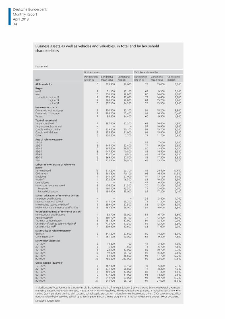
Business assets as well as vehicles and valuables, in total and by household characteristics

Figures in €

Item

Business assets Vehicles and valuables



Conditional median



Conditional median

All households 10 309,900 26,600 78 13,600 8,000

Regioneast1 7 51,100 17,100 69 9,300 5,000west 10 356,500 28,900 80 14,600 8,000



Type of householdSingle household 7 287,300 27,200 62 10,400 4,900Single-parent household – – – 57 10,900 1,900Couple without children 10 339,600 30,100 92 15,700 9,500Couple with children 15 335,500 21,900 91 15,400 9,500Other 6 130,200 7,700 77 11,700 5,600

Age of reference person16-24 – – – 55 7,000 3,90025-34 8 145,100 22,400 74 9,300 5,80035-44 10 195,600 18,500 80 13,400 8,00045-54 18 447,500 40,800 83 14,500 8,50055-64 12 272,000 9,500 86 14,700 8,50065-74 6 269,400 27,800 81 17,300 8,90075+ 2 327,300 36,500 66 13,700 5,300

Labour market status of reference personSelf-employed 79 315,200 23,700 83 24,400 10,600Civil servant 5 501,300 170,100 96 16,400 11,500Employee 7 341,100 27,000 84 13,100 8,000Worker5 4 272,200 46,300 82 10,800 6,900Unemployed – – – 47 6,300 1,900Non-labour force member6 3 176,000 21,300 70 13,300 7,000


School education of reference personNo school qualifi cations – – – 35 3,400 1,700Secondary general school 7 415,000 25,700 72 11,200 6,000Intermediate secondary school7 9 299,100 27,500 83 13,800 8,000Higher education entrance qualifi cation 13 263,800 26,000 81 16,000 8,800



Net wealth (quantile) 0- 20% 2 14,800 100 44 3,400 1,00020- 40% 3 5,300 1,600 73 6,700 4,80040- 60% 8 23,100 17,900 89 10,700 7,70060- 80% 12 49,200 26,100 89 15,200 9,80080- 90% 10 84,900 36,600 92 17,700 12,20090-100% 35 786,200 213,000 95 32,600 17,600



Deutsche Bundesbank


Current accounts, savings accounts (excluding private retirement provision) and building loan contracts, in total and by household characteristics

Figures in €

Item

Current accounts

Savings accounts (incl. savings under building loan accounts, excl. private retirement provisions) of which: building loan contracts



Condi-tional median



Condi-tional median



Condi-tional median

All households 99 7,100 1,800 70 27,600 9,900 31 9,800 5,000Regioneast1 99 4,200 1,400 61 18,000 5,900 24 7,000 4,500west 99 7,900 2,000 72 29,700 10,100 33 10,400 5,700

of which: region 12 99 7,600 1,600 71 23,200 8,300 28 7,100 4,500region 23 100 9,500 2,300 76 35,100 15,000 39 12,800 7,100region 34 99 5,900 1,300 67 26,000 7,800 28 7,900 5,000

Homeowner statusOwner without mortgage 100 11,500 3,100 83 46,700 22,000 42 12,100 7,900Owner with mortgage 100 9,300 2,500 82 18,800 9,600 47 9,900 5,400Tenant 99 4,300 1,000 59 18,500 4,900 21 7,600 4,000Type of householdSingle household 99 6,000 1,400 62 22,500 7,100 22 8,200 4,700Single-parent household 91 3,200 300 54 8,200 1,900 16 5,600 3,100Couple without children 100 8,600 2,400 77 35,200 13,900 38 9,400 5,800Couple with children 99 8,000 1,800 75 25,500 9,600 40 13,400 6,000Other 99 5,100 1,100 70 23,000 9,700 36 8,000 4,400Age of reference person16-24 98 2,600 1,000 60 4,200 1,200 17 5,000 2,00025-34 98 5,100 1,400 67 13,600 4,100 33 6,200 2,80035-44 98 7,000 1,500 71 22,900 7,500 35 11,100 4,90045-54 99 9,400 2,000 68 25,300 8,200 38 9,800 5,10055-64 100 6,000 1,900 69 36,200 18,400 36 12,600 6,90065-74 99 8,900 1,900 73 43,600 18,900 26 10,500 7,10075+ 100 7,100 2,000 72 30,400 14,000 21 8,400 5,600Labour market status of reference personSelf-employed 99 18,800 3,000 60 40,400 9,900 23 23,500 7,100Civil servant 100 8,600 3,200 86 38,600 20,200 53 12,300 7,000Employee 99 6,900 2,000 77 23,300 7,900 40 9,500 4,800Worker5 99 3,600 1,100 64 13,000 5,400 37 6,100 4,200Unemployed 97 2,000 100 27 14,600 1,900 9 4,600 2,000Non-labour force member6 99 6,600 1,900 67 34,500 13,100 23 9,400 6,600

Pensioner 99 6,900 2,000 71 35,800 15,100 23 10,000 7,000Retired civil servant 100 9,800 3,200 79 42,700 22,100 27 12,200 8,900

School education of reference personNo school qualifi cations 95 1,100 100 35 8,700 4,100 – – –Secondary general school 99 5,300 1,200 64 25,300 9,700 25 8,200 5,000Intermediate secondary school7 99 5,300 1,500 70 21,100 7,000 35 7,800 4,700Higher education entrance qualifi cation 100 10,800 2,800 77 35,000 12,700 36 12,600 5,900Vocational training of reference personNo vocational qualifi cations 98 2,500 400 50 12,600 3,000 14 7,500 3,400Apprenticeship8 99 5,100 1,500 69 22,000 7,900 33 8,900 5,000Technical college degree 100 9,000 2,300 79 35,300 16,400 40 10,100 5,800University of applied sciences degree9 100 10,500 2,900 78 39,000 15,700 37 11,600 4,800University degree10 100 15,700 4,700 78 41,500 18,400 34 12,300 7,800Nationality of reference personGerman 99 7,700 2,000 72 29,200 10,000 33 10,000 5,700Other nationality 97 3,300 400 48 15,600 4,600 18 9,900 3,200Net wealth (quantile) 0- 20% 97 700 100 35 1,600 500 8 2,400 1,10020- 40% 99 2,500 1,400 63 5,500 3,900 22 3,500 2,60040- 60% 100 5,300 2,100 79 17,700 9,900 37 8,000 4,90060- 80% 100 7,100 2,300 85 28,900 16,600 43 10,000 7,50080- 90% 100 12,100 4,300 90 46,500 24,500 49 10,000 6,70090-100% 100 27,100 8,700 83 78,400 37,300 43 21,700 9,700Gross income (quantile) 0- 20% 97 2,900 500 46 15,400 3,400 10 7,200 3,90020- 40% 99 4,700 1,000 61 19,400 7,500 21 6,700 5,80040- 60% 99 4,400 1,500 74 22,700 7,900 34 6,900 3,90060- 80% 100 6,700 2,000 81 26,000 9,700 44 8,500 4,90080- 90% 100 10,200 3,600 84 36,600 17,000 45 10,800 7,80090-100% 100 23,000 7,300 88 54,200 24,300 49 19,000 7,900


Deutsche Bundesbank


April 2019 35

Mutual fund shares (excluding private retirement provision), shares and bonds, in total and by household characteristics

Figures in €

Item

Mutual fund shares(excl. private retirement provision) Shares Bonds



Condi-tional median



Condi-tional median



Condi-tional median

All households 16 37,500 12,900 11 43,700 9,900 3 43,200 15,100

Regioneast1 10 36,000 14,100 5 27,400 7,700 1 32,500 17,300west 17 37,800 12,900 13 45,300 9,900 4 44,000 14,400


Homeowner statusOwner without mortgage 23 54,500 20,800 17 69,800 16,400 6 62,800 26,400Owner with mortgage 19 22,300 7,400 15 23,800 5,700 4 20,500 5,400Tenant 11 29,300 9,800 7 24,800 9,500 2 28,400 10,900

Type of householdSingle household 14 38,800 13,100 9 39,600 9,800 2 28,700 6,300Single-parent household – – – – – – – – –Couple without children 20 43,400 15,000 14 46,300 12,300 4 57,900 27,000Couple with children 14 24,900 7,100 12 48,600 7,800 4 27,100 5,800Other 15 11,200 4,000 8 38,400 13,800 4 39,400 9,900

Age of reference person16-24 – – – – – – – – –25-34 11 13,500 5,800 9 7,500 2,800 2 7,300 4,80035-44 16 19,900 5,500 8 51,200 4,800 4 30,600 7,30045-54 18 26,000 10,500 16 25,400 8,100 3 26,900 6,00055-64 19 38,900 14,800 10 50,300 11,400 3 42,200 23,70065-74 19 68,500 25,700 13 53,300 15,100 5 70,100 21,80075+ 11 69,500 32,400 12 79,500 27,600 3 66,900 27,900

Labour market status of reference personSelf-employed 21 47,200 14,600 14 41,800 6,800 4 32,800 3,500Civil servant 27 17,900 8,900 18 22,300 8,700 4 12,000 8,800Employee 20 24,700 7,700 12 32,900 9,600 4 31,700 9,700Worker5 7 20,500 9,300 4 3,500 1,100 – – –Unemployed 6 27,500 3,400 – – – – – –Non-labour force member6 13 61,300 24,800 11 63,100 16,300 3 63,100 23,800


School education of reference personNo school qualifi cations – – – – – – – – –Secondary general school 8 50,900 19,000 6 37,200 15,700 2 40,400 22,400Intermediate secondary school7 15 32,600 10,000 10 35,100 8,300 2 48,500 11,100Higher education entrance qualifi cation 25 35,600 12,100 17 49,900 9,700 5 42,200 11,500

Vocational training of reference personNo vocational qualifi cations 5 62,700 21,100 4 46,500 8,700 – – –Apprenticeship8 12 38,500 10,000 8 33,800 9,900 3 38,200 19,700Technical college degree 18 29,500 10,000 13 49,400 10,100 2 25,000 6,600University of applied sciences degree9 24 27,500 8,500 17 25,600 8,600 5 58,900 13,900University degree10 32 38,200 17,100 22 61,500 13,400 8 49,100 14,300

Nationality of reference personGerman 17 38,000 14,900 12 43,400 9,900 4 42,700 15,600Other nationality 8 38,700 5,900 2 88,300 61,900 0 119,100 16,200

Net wealth (quantile) 0- 20% – – – – – – – – –20- 40% 6 4,700 2,600 2 5,800 1,900 – – –40- 60% 17 13,500 8,100 9 13,400 5,400 2 13,700 10,30060- 80% 19 23,700 9,900 12 16,400 5,800 4 11,800 3,80080- 90% 34 41,000 21,600 26 28,400 10,600 6 39,000 24,20090-100% 39 79,100 38,600 36 93,700 23,500 12 82,400 38,400

Gross income (quantile) 0- 20% 4 21,300 7,600 3 21,200 10,700 1 15,400 4,20020- 40% 9 50,200 18,000 4 30,300 20,400 1 69,800 24,50040- 60% 15 34,100 13,700 10 30,400 8,000 2 23,600 11,10060- 80% 19 29,100 9,700 11 35,500 9,800 3 30,900 12,30080- 90% 25 25,000 9,100 18 31,400 5,900 7 35,900 5,30090-100% 36 54,500 19,400 34 70,800 14,200 11 58,100 24,900


Deutsche Bundesbank


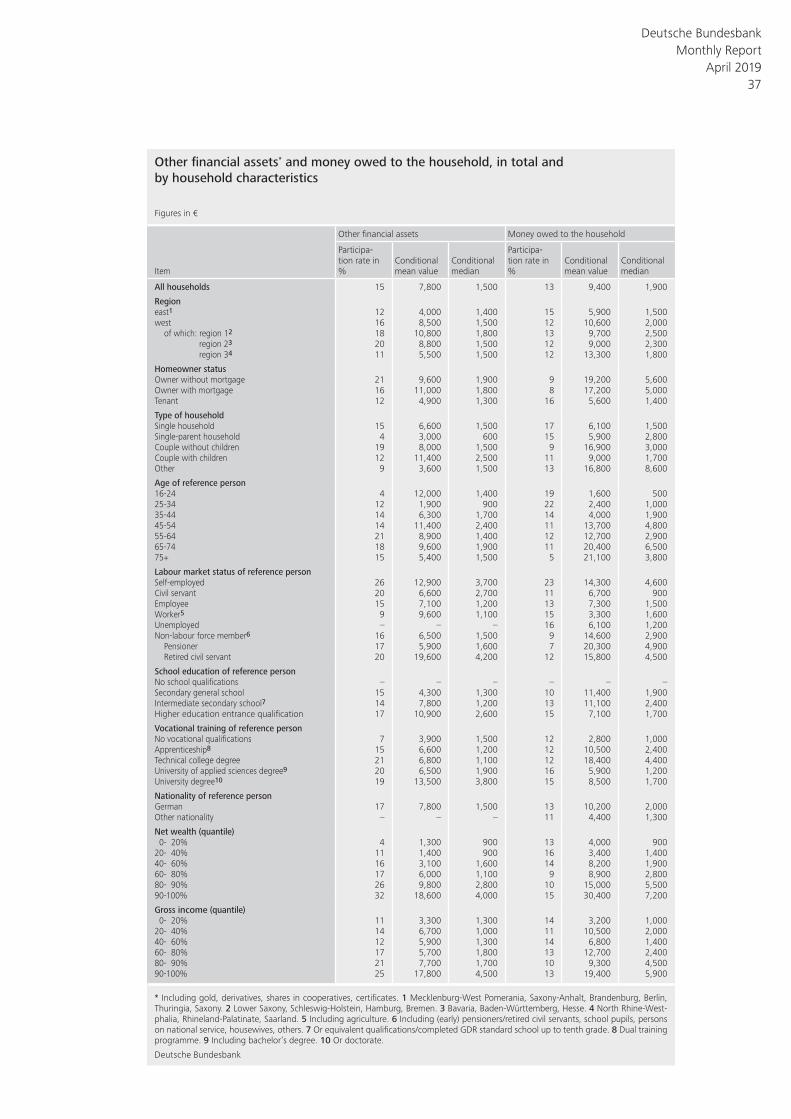
Other fi nancial assets* and money owed to the household, in total and by household characteristics

Figures in €

Item

Other fi nancial assets Money owed to the household



Conditional median



Conditional median

All households 15 7,800 1,500 13 9,400 1,900

Regioneast1 12 4,000 1,400 15 5,900 1,500west 16 8,500 1,500 12 10,600 2,000



Type of householdSingle household 15 6,600 1,500 17 6,100 1,500Single-parent household 4 3,000 600 15 5,900 2,800Couple without children 19 8,000 1,500 9 16,900 3,000Couple with children 12 11,400 2,500 11 9,000 1,700Other 9 3,600 1,500 13 16,800 8,600

Age of reference person16-24 4 12,000 1,400 19 1,600 50025-34 12 1,900 900 22 2,400 1,00035-44 14 6,300 1,700 14 4,000 1,90045-54 14 11,400 2,400 11 13,700 4,80055-64 21 8,900 1,400 12 12,700 2,90065-74 18 9,600 1,900 11 20,400 6,50075+ 15 5,400 1,500 5 21,100 3,800

Labour market status of reference personSelf-employed 26 12,900 3,700 23 14,300 4,600Civil servant 20 6,600 2,700 11 6,700 900Employee 15 7,100 1,200 13 7,300 1,500Worker5 9 9,600 1,100 15 3,300 1,600Unemployed – – – 16 6,100 1,200Non-labour force member6 16 6,500 1,500 9 14,600 2,900


School education of reference personNo school qualifi cations – – – – – –Secondary general school 15 4,300 1,300 10 11,400 1,900Intermediate secondary school7 14 7,800 1,200 13 11,100 2,400Higher education entrance qualifi cation 17 10,900 2,600 15 7,100 1,700


Nationality of reference personGerman 17 7,800 1,500 13 10,200 2,000Other nationality – – – 11 4,400 1,300

Net wealth (quantile) 0- 20% 4 1,300 900 13 4,000 90020- 40% 11 1,400 900 16 3,400 1,40040- 60% 16 3,100 1,600 14 8,200 1,90060- 80% 17 6,000 1,100 9 8,900 2,80080- 90% 26 9,800 2,800 10 15,000 5,50090-100% 32 18,600 4,000 15 30,400 7,200


* Including gold, derivatives, shares in cooperatives, certifi cates. 1 Mecklenburg-West Pomerania, Saxony-Anhalt, Brandenburg, Berlin, Thuringia, Saxony. 2 Lower Saxony, Schleswig-Holstein, Hamburg, Bremen. 3 Bavaria, Baden-Württemberg, Hesse. 4 North Rhine-West-phalia, Rhineland-Palatinate, Saarland. 5 Including agriculture. 6 Including (early) pensioners/retired civil servants, school pupils, persons on national service, housewives, others. 7 Or equivalent qualifi cations/completed GDR standard school up to tenth grade. 8 Dual training programme. 9 Including bachelor’s degree. 10 Or doctorate.

Deutsche Bundesbank


April 2019 37

Private retirement provision and whole life insurance policies as well as Riester/Rürup retirement provision products, in total and by household characteristics

Figures in €

Item

Private retirement provision (incl. whole life insurance policies)

of which: Riester/Rürup retirement provision products



Conditional median



Conditional median

All households 43 33,200 15,400 21 13,800 7,100

Regioneast1 37 21,100 10,800 20 10,100 5,400west 45 35,800 17,500 21 14,800 7,600




Age of reference person16-24 35 3,400 1,900 13 2,200 1,10025-34 44 10,500 4,700 23 6,500 2,90035-44 57 26,000 16,000 35 11,000 6,60045-54 63 47,400 26,600 34 18,600 9,70055-64 54 43,900 27,200 21 16,500 9,60065-74 19 34,500 19,000 5 15,500 5,00075+ 13 18,400 9,400 1 23,800 14,900

Labour market status of reference personSelf-employed 57 64,100 35,000 22 27,400 11,600Civil servant 71 32,900 22,900 42 11,900 6,800Employee 61 33,400 16,700 32 14,200 7,200Worker5 52 20,900 9,600 28 8,600 5,400Unemployed 29 25,000 6,400 14 6,700 6,200Non-labour force member6 19 28,000 12,800 5 11,900 7,600


School education of reference personNo school qualifi cations – – – – – –Secondary general school 31 27,000 10,000 11 10,300 6,700Intermediate secondary school7 50 29,400 14,000 26 10,000 5,900Higher education entrance qualifi cation 52 40,300 20,800 26 18,700 9,700



Net wealth (quantile) 0- 20% 16 3,600 1,500 7 3,300 1,60020- 40% 37 7,200 5,500 20 5,000 3,80040- 60% 53 19,700 14,300 23 9,800 6,40060- 80% 51 35,700 24,700 24 16,000 9,60080- 90% 54 49,800 33,500 28 18,600 10,90090-100% 64 82,300 59,500 29 28,400 17,500



Deutsche Bundesbank


Mortgage loans for owner-occupied and other properties and unsecured loans*, in total and by household characteristics

Figures in €

Item

Mortgage loans for owner-occupied properties

Mortgage loans for other properties Unsecured loans



Condi-tional median



Condi-tional median



Condi-tional median

All households 17 99,400 76,200 6 151,500 80,100 33 10,800 4,900Regioneast1 12 91,500 65,500 3 92,500 61,200 39 10,800 4,100west 19 100,600 78,000 7 157,500 86,100 31 10,800 4,900


Homeowner statusOwner without mortgage – – – 8 193,800 69,200 18 17,400 7,000Owner with mortgage 100 99,400 76,200 13 132,900 86,900 40 9,900 4,500Tenant – – – 3 118,300 86,800 37 9,500 4,600Type of householdSingle household 8 77,500 59,000 4 125,600 79,300 27 11,400 4,500Single-parent household 14 114,200 107,200 – – – 46 5,500 2,200Couple without children 19 91,000 67,700 7 124,100 72,100 31 11,100 5,000Couple with children 37 119,100 97,900 9 192,100 94,700 47 11,300 5,400Other 10 77,200 76,400 – – – 35 7,400 4,700Age of reference person16-24 – – – – – – 41 8,200 4,90025-34 8 184,300 166,100 2 202,500 130,100 51 10,200 5,10035-44 27 116,000 105,400 6 176,600 103,800 45 11,500 4,10045-54 33 97,500 72,600 9 133,700 89,600 38 12,600 5,80055-64 22 73,700 58,900 10 157,100 67,700 30 11,400 4,30065-74 9 72,800 60,300 5 158,000 42,500 18 5,100 2,00075+ 3 38,800 23,200 2 97,600 65,400 6 10,900 3,400Labour market status of reference personSelf-employed 27 105,200 72,200 17 197,600 109,200 36 14,200 6,700Civil servant 31 128,500 87,300 4 147,000 93,300 36 18,500 8,500Employee 25 106,900 83,800 7 150,100 79,300 41 11,700 5,500Worker5 23 77,000 69,000 5 107,900 62,500 47 10,900 4,200Unemployed – – – – – – 36 4,600 1,100Non-labour force member6 6 69,200 45,400 3 130,600 52,800 19 7,600 2,500


School education of reference personNo school qualifi cations – – – – – – 33 5,100 700Secondary general school 11 75,600 65,800 4 125,800 59,300 24 9,500 4,000Intermediate secondary school7 21 94,700 70,100 5 120,200 69,800 41 9,800 4,000Higher education entrance qualifi cation 21 116,900 97,100 9 179,700 96,000 33 13,000 6,300Vocational training of reference personNo vocational qualifi cations 8 88,800 68,900 2 174,600 121,800 36 6,600 2,500Apprenticeship8 18 84,100 69,300 4 125,300 64,900 34 10,300 4,000Technical college degree 22 112,500 92,100 9 145,400 96,400 28 13,500 5,200University of applied sciences degree9 19 113,500 95,000 6 126,000 104,800 32 14,200 7,000University degree10 21 130,100 99,500 12 186,900 91,000 27 15,200 7,500Nationality of reference personGerman 18 99,700 79,000 6 152,700 75,900 31 11,200 4,900Other nationality 16 90,500 63,400 4 127,700 85,800 45 9,700 4,500Net wealth (quantile) 0- 20% 3 154,300 139,200 2 349,600 180,300 53 11,300 4,90020- 40% 3 88,000 72,700 – – – 33 6,900 3,70040- 60% 20 96,100 77,600 3 105,600 96,200 33 8,500 5,30060- 80% 31 86,700 65,100 7 76,900 49,200 24 13,400 6,70080- 90% 27 100,400 84,300 9 98,300 87,900 20 17,000 5,30090-100% 30 121,500 87,900 24 203,600 98,600 20 16,800 2,500Gross income (quantile) 0- 20% 2 76,600 47,200 – – – 27 6,200 2,70020- 40% 7 62,800 39,400 2 91,800 69,000 31 8,900 3,50040- 60% 15 82,700 62,700 3 122,200 55,600 37 10,800 5,30060- 80% 25 91,900 76,800 7 114,600 56,600 37 12,500 6,90080- 90% 37 102,500 78,600 11 129,600 106,100 36 11,200 4,60090-100% 37 136,600 103,500 21 211,400 98,400 26 19,900 7,800

* Including consumer loans, student loan debt, revolving credit card debt. 1 Mecklenburg-West Pomerania, Saxony-Anhalt, Brandenburg, Berlin, Thuringia, Saxony. 2 Lower Saxony, Schleswig-Holstein, Hamburg, Bremen. 3 Bavaria, Baden-Württemberg, Hesse. 4 North Rhine-Westphalia, Rhineland-Palatinate, Saarland. 5 Including agriculture. 6 Including (early) pensioners/retired civil servants, school pupils, persons on national service, housewives, others. 7 Or equivalent qualifi cations/completed GDR standard school up to tenth grade. 8 Dual training programme. 9 Including bachelor’s degree. 10 Or doctorate.

Deutsche Bundesbank


April 2019 39

Gross and net income,* in total and by household characteristics

Figures in €

Item

Gross income (annual, calculated from components)

Net income (annual, self-assessment)

Mean value Median Mean value Median

All households 53,000 40,100 36,700 27,600

Regioneast1 42,000 32,200 30,200 23,800west 56,000 42,400 38,500 29,800

of which: region 12 51,000 40,900 35,500 26,200region 23 63,400 46,700 42,000 31,500region 34 49,300 38,900 35,700 27,200

Homeowner statusOwner without mortgage 62,300 46,200 44,100 32,200Owner with mortgage 81,800 66,900 48,700 41,600Tenant 39,800 30,200 29,500 22,200

Type of householdSingle household 31,800 25,000 26,000 18,600Single-parent household 32,200 25,200 22,200 20,900Couple without children 67,000 52,700 46,200 35,700Couple with children 80,200 61,700 47,000 41,200Other 48,700 37,300 31,900 28,200

Age of reference person16-24 20,000 12,800 16,000 11,90025-34 42,300 37,600 29,400 25,10035-44 61,500 51,700 38,400 35,00045-54 74,900 55,200 41,800 34,90055-64 60,900 47,300 41,800 29,90065-74 43,900 32,200 39,900 25,70075+ 34,400 27,900 33,100 21,900

Labour market status of reference personSelf-employed 81,600 55,300 56,300 33,400Civil servant 78,900 67,300 59,700 47,700Employee 67,300 53,100 39,300 34,700Worker5 45,400 42,000 31,400 28,600Unemployed 25,100 19,500 14,600 12,800Non-labour force member6 36,500 28,200 32,500 22,700

Pensioner 35,500 27,800 34,800 22,700Retired civil servant 54,000 47,900 40,600 34,500

School education of reference personNo school qualifi cations 20,000 17,200 22,900 12,700Secondary general school 40,000 30,700 30,300 22,700Intermediate secondary school7 51,600 42,000 35,500 29,800Higher education entrance qualifi cation 69,300 54,100 45,000 34,700

Vocational training of reference personNo vocational qualifi cations 28,000 21,900 21,000 17,300Apprenticeship8 48,200 37,600 33,400 25,100Technical college degree 60,100 49,500 37,600 32,000University of applied sciences degree9 66,900 50,200 40,300 34,900University degree10 81,700 68,300 60,000 38,100

Nationality of reference personGerman 54,500 41,400 37,900 28,800Other nationality 45,100 34,400 28,700 22,800

Net wealth (quantile) 0- 20% 25,800 20,300 18,900 15,20020- 40% 34,200 31,600 29,800 22,70040- 60% 50,100 44,100 34,500 29,80060- 80% 63,700 50,900 43,500 33,00080- 90% 73,600 60,500 47,300 38,80090-100% 109,600 85,100 66,900 50,000

Gross income (quantile) 0- 20% 11,400 12,200 14,700 12,00020- 40% 26,100 26,300 23,600 20,40040- 60% 40,100 40,100 32,800 26,80060- 80% 59,400 58,700 38,100 36,80080- 90% 86,100 85,100 57,300 47,80090-100% 170,800 137,300 92,000 65,800

* Gross income is the sum of the income components included in the survey. By contrast, net income is the respondent’s self-assessment of the total. When respondents are asked to give net income as an aggregate, aggregation bias may arise; this means that incomes are understated as certain income components are more likely to be forgotten than when they are specifi cally asked about. 1 Mecklenburg-West Pomerania, Saxony-Anhalt, Brandenburg, Berlin, Thuringia, Saxony. 2 Lower Saxony, Schleswig-Holstein, Hamburg, Bremen. 3 Bavaria, Baden-Württemberg, Hesse. 4 North Rhine-Westphalia, Rhineland-Palatinate, Saarland. 5 Including agriculture. 6 Including (early) pen-sioners/retired civil servants, school pupils, persons on national service, housewives, others. 7 Or equivalent qualifi cations/completed GDR standard school up to tenth grade. 8 Dual training programme. 9 Including bachelor’s degree. 10 Or doctorate.

Deutsche Bundesbank


List of references

Adam K. and P. Tzamourani (2016), Distributional consequences of asset price inflation in the euro

area, European Economic Review 89, pp. 172-192.

Ampudia, M., D. Georgarakos, J. Slacalek, O. Tristani, P. Vermeulen and G.L. Violante (2018), Mon-

etary policy and household inequality, ECB Discussion Paper No 2170.

Auclert, A. (2019), Monetary policy and the redistribution channel, American Economic Review

(forthcoming).

Banca d’Italia (2018), Survey on Italian Household Income and Wealth, Statistics Report, 12 March

2018.

Brenke, K. (2014), Ostdeutschland – ein langer Weg des wirtschaftlichen Aufholens, DIW Wochen-

bericht 40/ 2014, pp. 939-957.

Casiraghi, M., E. Gaiotti, L. Rodano and A. Secchi (2016), A “Reverse Robin Hood”? The distribu-

tional implications of non- standard monetary policy for Italian households, Banca d’Italia Discus-

sion Paper No 1077.

Chakraborty, R. and S. R. Waltl (2018), Missing the wealthy in the HFCS: micro problems with

macro implications, ECB Working Paper 2163.

Deutsche Bundesbank (2019), The impact of an interest rate normalisation on the private non-

financial sector in the euro area from a balance sheet perspective, Monthly Report, January 2019,

pp. 13 ff.

Deutsche Bundesbank (2016a), Distributional effects of monetary policy, Monthly Report, Septem-

ber 2016, pp. 13 ff.

Deutsche Bundesbank (2016b), Household wealth and finances in Germany: results of the 2014

survey, Monthly Report, March 2016, pp. 57 ff.

Deutsche Bundesbank (2013), Household wealth and finances in Germany: results of the Bundes-

bank survey, Monthly Report, June 2013, pp. 23 ff.

Federal Reserve Bank (2017), Changes in U.S. Family Finances from 2013 to 2016: Evidence from

the Survey of Consumer Finances, Federal Reserve Bulletin 103 (3).

Fisher, J., D. Johnson, T. Smeeding and J. Thompson (2018), Inequality in 3D: Income, Consump-

tion and Wealth, Board of Governors of the Federal Reserve System Finance and Economics Dis-

cussion Series Working Paper 2018-001.

Gesamtverband der Deutschen Versicherungswirtschaft e.V. (2018), Statistical Yearbook of German

Insurance.


April 2019 41

Goldfayn- Frank, O. and J. Wohlfahrt (2018), How Do Consumers Adapt to a New Environment in

their Economic Forecasting? Evidence from the German Reunification, IMFS Working Paper No 129.

Grabka, M. and C. Westermeier (2014), Anhaltend hohe Vermögensungleichheit in Deutschland,

DIW Wochenbericht 9/ 2014, pp. 151-164.

Household Finance and Consumption Network (2016a), The Household Finance and Consumption

Survey: results from the second wave, ECB Statistics Paper 18/ 2016.

Household Finance and Consumption Network (2016b), The Household Finance and Consumption

Survey – Wave 2 – Statistical Tables.

Kindermann, F., J. Le Blanc, M. Piazzesi and M. Schneider (2019), Expectations during the German

House Price Boom, mimeo.

Le Blanc, J. and T. Schmidt (2019a), Do Homeowners Save more than Renters? – Evidence from the

German Wealth Survey, mimeo.

Le Blanc, J. and T. Schmidt (2019b), The joint distribution of income, wealth and consumption in

Germany, mimeo.

Lenza, M. and J. Slacalek (2019), How does monetary policy affect income and wealth inequality?

Evidence from quantitative easing in the euro area, ECB Working Paper No 2190.

Marek, P. (2017), Saving patterns in the low- interest- rate setting – results of the 2016 PHF summer

survey, Deutsche Bundesbank Research Brief 12-4/ 2017.

Oesterreichische Nationalbank (2019), Eurosystem Household Finance and Consumption Survey

2017 – First Results for Austria.

Pasteau, E. and J. Zhu (2018), Love and money with inheritance: marital sorting by labor income

and inherited wealth in the modern partnership, Deutsche Bundesbank Discussion Paper No 23/

2018.

Piketty, T. (2014), Capital in the Twenty- First Century, Harvard University Press.

Saez, E. and G. Zucman (2016), Wealth Inequality in the United States since 1913: Evidence from

Capitalized Income Tax Data, Quarterly Journal of Economics 131(2), pp. 519-578.

Tzamourani, P. (2019), The interest rate exposure of euro area households, Deutsche Bundesbank

Discussion Paper No 01/ 2019.

Vermeulen, P. (2018), How fat is the top tail of the wealth distribution?, Review of Income and

Wealth 64(2), pp. 357-387.

Vermeulen, P. (2016), Estimating the top tail of the wealth distribution, American Economic Review

106(5), pp. 646-650.


household wealth and finances in germany: results …...life insurance policies are also included.2...

Documents