How Well are Earnings Measured in the Current Population Survey?

Bias from Nonresponse and Proxy Respondents*

Christopher R. Bollinger Department of Economics

University of Kentucky Lexington, KY 40506

Voice: (859)257-9524 Fax: (859)323-1920 e-mail: crboll@email.uky.edu

hompage: http://gatton.uky.edu/faculty/bollinger

Barry T. Hirsch Department of Economics

Trinity University San Antonio, TX 78212-7200

Voice: (210)999-8112 Fax: (210)999-7255 e-mail: bhirsch@trinity.edu

homepage: http://www.trinity.edu/bhirsch

April 2007

Earnings nonresponse is currently about 30% in the CPS-ORG and 20% in the March CPS. Census imputes missing earnings by assigning nonrespondents the reported earnings of matched donors. Even if nonresponse is random, in a wage equation there exists severe “match bias” on coefficients attached to non-match imputation attributes (union status, industry, foreign-born, etc.) and imperfectly matched criteria (schooling, age, etc.). Bollinger-Hirsch (JOLE, July 2006) show that if nonresponse is conditional missing at random (i.e., ignorable nonresponse) then unbiased wage equation estimation can be achieved in several ways, most easily by deleting imputed earners from the sample. The focus of this paper is twofold. First, we examine whether or not nonresponse is ignorable in the CPS-ORG and March CPS. Second, we assess the effect of “proxy” respondents on earnings, since roughly half of CPS records are based on self-responses and half on responses from another household member. Earnings nonresponse varies little with respect to most earnings attributes, but is noticeably highest among those in the top percentiles of the predicted earnings distribution. Wage effects due to nonresponse and proxy reports are estimated using selection models and longitudinal analysis. Based on reasonable instruments to identify selection, we conclude that there is negative selection into response among men, but relatively little selection among women. Wage equation slope coefficients are affected little by selection (as compared to OLS results for respondent-only samples), but because of intercept shifts, our preliminary evidence suggests that men’s (but not women’s) wages are understated due to response bias by as much as 10%. By contrast, longitudinal results from the ORG suggest moderate response bias for women as well as men. OLS estimate of proxy effects on reported earnings indicates a modest negative effect (about 2-3%). What this masks, however, is large negative correlations between non-spousal proxy reports and earnings, combined with spousal proxy reports of earnings roughly equivalent to self-reports. The panel analysis indicates that much of the (non-spousal) proxy effect on earnings seen in cross-sectional analysis is due to worker heterogeneity or fixed effects (including selection into response, which is correlated with proxy reports). In short, proxy reports by spouses and non-spouses are only about 1-2% lower than are self-reports from these same individuals, but workers whose earnings are reported by non-spousal household members tend to have even lower wages for reasons not reflected by measured characteristics. *For North American Summer Meetings of the Econometric Society, Duke University, June 21-24, 2007.

Introduction

The Current Population Survey (CPS) is used extensively by economists and other social

scientists because of its large sample size, comprehensiveness, historical continuity, and timeliness. The

American Social and Economic Supplement (ASES) to the March CPS is often used for estimation of

annual earnings equations based on earnings in all jobs the previous calendar year, while the monthly

CPS Outgoing Rotation Group (ORG) files are used for estimation of hourly earnings equations for wage

and salary workers based on the principal job the previous week.

Although item nonresponse rates are low for most questions in the CPS, the notable exception is

for questions on income and earnings. Currently, about 30% of employed wage and salary workers in the

CPS-ORG do not provide earnings information. Missing earnings are assigned (allocated) to

nonrespondents using a cell hot deck imputation procedure. The procedure matches nonrespondents with

the “donor” earnings of the most recent respondent who has an identical set of match characteristics

(Hirsch and Schumacher 2004). In the March ASES, about 20% of individuals employed the previous

year fail to report annual earnings. Their earnings are assigned using a sequential hot deck procedure.

This procedure begins its search for an earnings donor using a relatively detailed set of match attribute

values and then, failing to find a match, begins collapsing categories (say from a narrowly defined to a

broader age range) until a matching donor is found from that same month’s survey (Lillard, Smith, and

Welch 1986).

Hirsch and Schumacher (2004) and Bollinger and Hirsch (2006) have established that even if

nonresponse is perfectly random, the imputation procedure can result in a severe “match bias” in

regression settings. Specifically, wage regression coefficients on attributes that are not match criteria

(union, industry, foreign-born, etc.) are biased toward zero by roughly the nonresponse (imputation) rate.

Coefficients on imperfectly matched attributes such as education can also be severely biased. For

example, estimated returns to the GED are overstated because nonrespondents with a GED are typically

assigned the earnings of donors with a standard high school degree or some college).1 Bollinger and

Hirsch (2006) examine alternative methods to account for match bias, the simplest of which is to

removing those with imputed earnings (nonrespondents) from the estimation sample. But this and other

approaches assume that nonresponse is either random or ignorable (i.e., equivalent expected earnings for

respondents and nonrespondents, conditional upon regressors in the model). Unfortunately, we have

surprisingly little information as to whether or not nonresponse is conditional missing at random and thus

ignorable. Moreover, earnings nonresponse has risen over time in the CPS, making the question of

possible response bias increasingly important.

1 For analysis of the effect of imputation on estimates of the returns to the GED, see Heckman-and LaFontaine (2006) and Bollinger and Hirsch (2006).

1

The purpose of this paper is twofold. A principal goal is to examine the issue of response bias. Is

there nonignorable response bias in the ORG and ASES CPS earnings files? If so, what is its nature and

severity? How might researchers correct for the bias? We address the structure and impact of earnings

nonresponse using both the CPS ORG and ASES data files for 1998 through 2006. We employ two

alternative approaches. One approach focuses on the selection of appropriate instruments accounting for

response, thus permitting estimation of selection adjusted wage equations. Our other approach is the use

of longitudinal analysis that identifies the effects of response bias from workers who report earnings in

one year but who do not respond and are assigned donor earnings in a second year.

A second goal of the paper is to assess the impact of “proxy” reporting of earnings. About half of

all CPS individual records are based on self responses, while the other half rely on the responses of

another household member (a proxy), often a spouse. It is commonly believed that proxy reports have

little effect on earnings or wage regression coefficients (Angrist and Krueger 1999), although this topic

has not received much attention. The issue of proxy respondents is important for several reasons. Given

that half of earnings responses are from proxies, the question of whether or not proxy reporting affects

wages is important in its own right. In addition, because proxy respondents are less likely to report

earnings than are self-respondents, the presence of a proxy respondent potentially provides an appropriate

instrument to assess whether nonresponse is ignorable. But its appropriateness as an instrument depends

on whether it has a direct effect on the wage, conditional on other wage regressors. If proxy status affects

earnings nonresponse but not the wage, it may facilitate a reasonable way to control not only for response

bias, but also to correct for match bias associated with imperfect earnings imputation. If proxy

respondents affect reported wages to a substantial degree, however, then these effects should no longer be

ignored in analyses of earnings based on the CPS.

Response Bias and Proxy Effects on Earnings: What is Known?

Several studies use validation studies to evaluate the accuracy of measured earnings. These

studies typically exclude nonrespondents with imputed earnings, but sometime do compare reported

earnings based on self-response versus a proxy household member. A small number of studies examine

the quality of imputed values and the issue of response bias.

Bound and Kruger (1991) conclude that proxies are about as accurate as self-respondents, based

on the 1977 and 1978 March CPS (measuring annual earnings the previous year) compared to earnings

reported in Social Security records. Comparing earnings reported in a January 1977 CPS supplement

with employer reports on earnings (the survey asked workers the name of their employer), Mellow and

Sider (1983) also conclude that self and proxy reports on earnings are similar. But a close look at their

results (Table 1) suggests that proxy respondents underreport wages by more and overreport hours a bit

2

less than do self respondents, the two reinforcing each other and producing about a small 2%

understatement in proxy relative to self reported wages (results are not reported separately by gender). In

regressions of the employer-employee difference in reported wages on typical wage determinants, they

find no significant coefficients.

Far less is known as to whether nonresponse in the CPS is ignorable and whether imputation does

a good job on average in estimating earnings. The little work of which we are aware focuses on the

March CPS files measuring annual earnings the previous year and not the monthly earnings files (the CPS

ORG files beginning in 1979) reported earnings and weeks worked on the principal job during the

previous week. Greenlees et al. (1982) examined the March 1973 CPS, comparing wage and salary

earnings the previous year with 1972 matched income tax records. They restrict their analysis to full-

time, full-year heads of households in the private nonagricultural sector whose spouse did not work. They

conclude that nonresponse is not ignorable, being negatively related to income (negative selection into

response). The authors estimate a standard wage equation using the administrative IRS earnings as the

dependent variable. Based on those values they impute earnings for those who are CPS nonrespondents.

Their imputations understate administrative wage and salary earnings by .077 log points. The sample

included only 561 nonrespondents (imputed values) and earnings were censored at $50,000. Herriot and

Spiers (1975) report similar Census results with these data, with the ratio of CPS respondent to IRS

earnings being .98 and of CPS imputed to IRS earnings being .91. These two figures taken together

suggest a downward response bias of .07, since imputed values are based on respondents with similar

characteristics. It is not clear whether such a large magnitude can be generalized outside this survey and

time period. The sequential hot deck procedure used in the March survey at that time was primitive as

compared to subsequent methods, for example, failing to use education as a match variable (Lillard et al.

1986). But the findings from this validation study suggest the importance of the question of whether or

not there exists nonignorable response bias, all the more so given increasing rates of nonresponse.

A more encouraging outcome emerges from the study by David et al. (1986), who examine a

similar validation study matching the March 1981 CPS and 1980 IRS reports. They conclude that the

Census hot deck does a reasonably good job in predicting earnings as compared to alternative imputation

methods. Their results are based on a broader sample and the use of a more detailed Census imputation

method than were the imputation methods considered in Greenlees et al (1982). David et al. note the

many difficulties in comparing CPS and IRS measures of income, not regarding either measure as a true

measure of earnings. They conclude that nonresponse is not ignorable; the earnings structure for

respondents providing an unreliable basis for predicting the earnings of nonrespondents. An interesting

finding is that imputations for single returns (relative to IRS values) are a good bit higher than imputed

values for joint returns (relative to IRS values), indicating that negative selection into response (i.e., that

3

imputations will understate true earnings) is most serious for married couples (the group considered by

Greenlees et al.). In short, the evidence available suggests that there exists at least modest response bias,

that it is likely to reflect negative selection into response, and that it may differ between those filing single

and joint returns. It is hard to know how these results based on March CPS records from more than 25

years ago apply to more current CPS earnings and imputation methods or to the CPS ORG earnings files.

We are unaware of prior work examining response bias in the monthly CPS ORG earnings files,

which begin in January 1979. The 1973-78 May CPS earnings supplements, a precursor to the ORGs, did

not include imputed earnings values.2 Using recent ORG files, Hirsch and Schumacher (2004, fn. 29)

estimate a selection wage equation model in which the proxy variable is used to identify

nonresponse (imputation). Based on similar union wage gap estimates from a full-sample

selection model and an OLS wage regression on the sample of earnings respondents, the authors

conclude that response bias is modest at most. Their principal concern is not response bias,

however, but the first-order problem of “match bias” in the union wage gap estimate resulting

from the inclusion of imputed earners in an OLS wage equation (or, more generally, match bias

with respect to coefficients on any attribute not used in the CPS imputation procedure). Hirsch

and Schumacher’s use of the proxy variable to identify a selection model was intended to

account for possible response bias in addition to correcting for the known match bias.3

A recent paper by Korinek, Mistiaen, and Ravallion (2005) examines potential bias from unit

nonresponse as opposed to earnings (item) nonresponse. Use of CPS weights is intended to account for

nonrandom survey nonparticipation. But such weights are predicated on the assumption that response is

nonrandom across geographic areas (states) but random within states. Korinek et al. question such an

assumption. They show that response rates across states vary inversely with income (and other

measurable factors), and apply this relationship to adjust weights within states.4 It seems reasonable that

negative selection in response might apply to item nonresponse as well as unit nonresponse. Our focus is

on item nonresponse with respect to earnings, its frequency being substantially greater than unit

nonresponse.

Although our summary of the literature is brief and selective, we believe it is fair to say that

evidence on response bias and proxy effects on earnings in the CPS is limited, involves largely older data

2 About 20% of the May 1973-78 records have missing earnings values, much of this due to nonresponse (Hirsch and Schumacher 2004). 3 Hirsch and Schumacher (2004, fn. 29) report a proxy coefficient of -.02 when included in an OLS wage equation. 4 We subsequently show that earnings nonresponse is substantially lower in rural areas and higher in large metropolitan areas, holding constant other earnings determinants. Thus, the inverse relationship between response and income found by Korinek et al. (2005) reflects to some degree the substantial earnings differences with respect to area size.

4

sets, and is far from conclusive. Proxy effects on earnings are generally believed to be minor (Angrist

and Krueger 1999), although there are hints in prior studies that proxy respondents report somewhat lower

earnings than do self-respondents. There is stronger evidence that there exists at least some level of

nonignorable response bias, the evidence pointing toward negative selection into response. Yet much of

this evidence is dated, from a period where nonresponse was less frequent (and overly sparse hot deck

procedures were used in the March CPS). There is little study of possible response bias in the CPS ORG,

a data source providing many advantages over the March CPS for the study of wage determination (see

Lemieux 2006), but which have higher rates of nonresponse than in the March surveys.

Data

Analysis in this paper uses the CPS Outgoing Rotation Group (ORG) monthly earnings files and

the March CPS Annual Social and Economic Supplement (ASES, previously known as the Annual

Demographic File or ADF). For both data sets, wage level equations are estimated using multiple cross

sections pooled across years, while wage change equations are estimated using pooled two year panels.

The panel data are made possible by the sample design of the CPS. Households are included in the CPS

for eight months -- four consecutive months in the survey, followed by eight months out, followed by four

months in. Thus, most CPS households are included during the same month in consecutive years.

The ORG files used are for 1998 through 2006. In addition to answering demographic and

employment questions asked of all households in the monthly CPS, an earnings supplement is

administered to the quarter sample of employed wage and salary workers in their outgoing 4th and 8th

months included in the survey (i.e., the outgoing rotation groups). The earnings supplement includes

questions on usual earnings in the principal job the previous week, usual hours worked per week in that

job, and worker union status in that job. Based on this information, one can form a measure of average

hourly earnings or the wage. Hourly workers report their straight-time wage rate. For hourly workers

who do not report tips, overtime pay, or commissions, the straight time wage is used as the hourly wage.

For all other workers, the wage is measured by usual weekly earnings (inclusive of tips, overtime, and

commissions) divided by usual hours worked per week on the principal job.5 For workers whose weekly

earnings are top-coded in the ORGs (at $2,885 or about $150,000 per year), we assign the estimated mean

above the cap based on the Pareto distribution (posted at www.unionstats.com).

The March CPS or ASES is used for 1998 through 2006. The March supplement is administered

to all rotation groups in the CPS. Earnings (and income) questions do not apply to the previous week, but

to the previous calendar year (1997-2005). A March wage measure can be calculated as annual earnings

5 For the small number of workers who do not report an hourly wage and report variable hours, the wage is calculated using hours worked the previous week.

5

for all wage and salary jobs divided by annual hours worked (the product of week worked and hours

worked per week). Most of our analysis with the March survey simply examines annual earnings among

full-time, full-year workers. This avoids confounding reporting errors (say from a proxy respondent) on

earnings with those on hours and weeks worked. Industry and occupation designation is based on the

longest job held the previous year. Union status is not measured for that job.

Rates of earnings nonresponse in the CPS are provided in Table 1 (for earlier rates for the ORGs,

see Hirsch and Schumacher 2004). Due to more intensive efforts to contact and acquire responses for the

ASES, nonresponse rates for the March ASES are lower than for the ORG (and are lower in the ORG in

March than in other months, as seen subsequently). In recent years, nonresponse in the ORG files has

been about 30% of the sample, versus about 20% in the March CPS (but 17.3% in 2006). Nonresponse

rates are about 1 percentage point higher if one applies employment weights to the sample. This

difference results from a combination of lower response rates in large metropolitan areas than in smaller

cities and non-metropolitan areas, and from Census procedures in which it samples a smaller proportion

of households (thus large employment weights) in highly populated areas and oversamples in less-

populated areas.

Individuals for whom earnings are not reported have earnings imputed (i.e., allocated) by the

Census. Different imputation procedures are used in the ORG and ASES.6 Earnings in the CPS-ORG are

imputed using a "cell hot deck" method. There has been minor variation in the hot deck match criteria

over time. For the ORG files during the 1998-2002, the Census created a hot deck or cells containing

14,976 possible combinations based on the product of the following seven categories: gender (2 cells),

age (6), race (2), education (3), occupation (13), hours worked – including whether or not hours per week

are variable (8), and receipt of tips, commissions or overtime (2). Beginning in 2003 when new

occupation and industry codes were adopted, the number of major occupation categories fell to 10,

reducing the number of hot deck combinations to 11,520. In the ORG, Census keeps all cells "stocked"

with a single donor, insuring that an exact match is always found. The donor in each cell is the most

recent earnings respondent surveyed previously by the Census with that exact combination of

characteristics. As each surveyed worker reports an earnings value, the Census goes to the appropriate

cell, removes the previous donor value, and "refreshes" that cell with a new earnings value from the

respondent. If a cell has not been stocked by a matching donor from the current survey month, Census

uses donor earnings obtained in from prior survey months (or years).7

6 Details on the ORG imputation procedure are provided by Hirsch and Schumacher (2004) and Bollinger and Hirsch (2006). Lillard, Smith, and Welch (1986) provide a detailed discussion of the March imputation method.. 7 For an analysis of “dated donors” and the bias from use of nominal earnings, see Bollinger and Hirsch (2006).

6

Hirsch and Schumacher (2004) and Bollinger and Hirsch (2006) have provide detailed analyses

of coefficient bias (match bias) in the ORGs. The intuition behind match bias is straightforward.

Characteristics which are not used in the imputation procedure are largely uncorrelated with the imputed

earnings. The resulting estimated coefficients are then an average of a value close to zero and the true

coefficient, the weights for the average being the respective proportions of observations which are and are

not imputed. As an illustration, suppose one is estimating the union-nonunion wage gap. Union status is

not an imputation match criterion. Hence, most union nonrespondents are assigned the earnings of

nonunion donors and some nonunion nonrespondents are assigned the earnings of union donors. The

union-nonunion wage gap among those with imputed earnings is close to zero (union status may be

correlated with wage determinants used as match criteria). Bollinger and Hirsch (2006, Table 2) report a

biased full-sample union wage gap estimate of .14 log points among men, a weighted average of a .19

estimate for earnings respondents and .02 among nonrespondents with imputed earnings. Attenuation of

the union coefficient in the full sample exceeds 25%, nearly as large as the 28.7% of the sample imputed.

Notably, alternative corrections for match bias, in particular estimation with the respondent only

sample, rely critically on the assumption that earnings are conditional missing at random; that is, response

bias is ignorable (Bollinger and Hirsch 2006). Hence this paper, which has as a goal the measurement of

response bias, may provide implications about how to deal with imputed earners and match bias.

The imputation procedure in the ASES differs from the ORG. The ASES use a "sequential"

rather than "cell" hot deck imputation procedure: Nonrespondents are matched to donors from within the

same March survey in sequential steps, each step involving a less detailed match requirement. The

matching program first attempts to find a match on the exact combination of variables using the full set of

match characteristics (similar to those used in the ORG). Absent a successful match at that level,

matching proceeds to a next step with a less detailed breakdown, for example, broader occupation and age

categories. As emphasized by Lillard, Smith, and Welch (1986), the probability of a close match declines

the less common an individual's characteristics.

The CPS typically interviews one individual who provides responses for all household members.

Thus, approximately half of all individuals have recorded responses that are self-reported and about half

have responses that are reported by another household member, referred to here as “proxy” respondents.

Among those records based on proxy responses, over half are from a spouse. As reported in Table 2. the

frequency of proxies and spouse proxies differs by gender. Using as an example the ORGs, 59% of male

earnings records are based on a proxy respondent of whom 35% are wives (i.e., 59% of men’s proxies are

a spouse). Among women’s earnings records, 41.5% are based on a proxy of whom 21% are husbands

(50% of women’s proxies are a spouse). Below we examine how rates of earnings nonresponse differ

between earnings records based on self and proxy respondents, as well as other measured attributes.

7

Who Fails to Report Earnings?

Response Rates and Worker Attributes. Our paper examines the role of response bias and proxy

respondents on earnings in the CPS. In this section we examine correlates of earnings nonresponse, the

existence of a proxy household respondent being the most important. We first examine response

determinants that are potential instruments for use in a selection wage model (i.e., response determinants

not correlated with the wage). For both the ORGs and ASES we consider the proxy variable, for the

ORGs the calendar month of the survey, and for the ASES the CPS rotation group.8

Returning to Table 1, we see that when an earnings record is based on self-reports rather than a

proxy interview, nonresponse (imputation) rates are 24.1% in the 1998-2006 ORG. When the interview is

a proxy household member, earnings nonresponse is 35.4%, 11 percentage points higher. When the

proxy household member is a spouse, however, nonresponse is 30.1, “only” 6 percentage points higher

than nonresponse among self-reporters. A similar pattern is found for the March supplements, where

earnings nonresponse rates are about 8 percentage points higher for proxy than self-respondents (but just

3 percentage points for spouse proxies). The importance of proxy interviews as a determinant of earnings

nonresponse suggests that proxy is a strong candidate to be used as an instrument to account for selection

into response. This requires that a proxy response has little effect on earnings, an issue we examine.

Other candidates for instruments are identified in Table 1. We find that nonresponse rates for the

February and March ORG interviews are lower than for all other months by about 4 percentage points

(roughly 25% or 26% versus 30%; again, highly significant statistically). There is little variation in

nonresponse among the other 10 months. We speculate that this is related to the lower rates associated

with the ASES interviews, which go into the field in February and March. It is not entirely clear by what

mechanism this occurs, as those in the ORG in February should not be in the March ASES, and some of

the March ASES is collected into the beginning of April which does not exhibit a differential response.

Alternative explanations exist. Nonresponse may come from two sources. First, and perhaps

most obviously, nonresponse may simply indicate an individual’s unwillingness to share what they

consider to be personal information. A second source is lack of knowledge. We expect that proxy

interviews are less likely to respond because of lack of knowledge. It may be that in February and March

people are more aware of income amounts because of tax documents and this explains the higher response

rates in the ORG (and the ASES overall, which is administered in March because it is during tax season).

Were knowledge of earnings the key explanation, however, we might expect some of this “knowledge” to

be retained in April and perhaps later months, yet we see no such evidence. Nor is it obvious that tax

8 We considered using as instruments information from CPS supplements on voting behavior and volunteer activity on the expectation that “public spirit” would increase the likelihood of survey response, but have no direct effect on the wage. Volunteer activity but not voting was found to be associated with a higher probability of earnings response. Both of these potential instruments were significantly correlated with the wage.

8

knowledge is critical for the ORGs, since ORG earnings questions concern hours worked and rates of pay

at the principal job during the prior week. An alternative possibility is that that bad weather or other

seasonal factors reduce costs of participating in the study and improve earnings response.

For households in the March survey who are in either their first or fifth month in sample, the

nonresponse rate is about 2 percentage points lower (because of the large samples, the differences are

highly statistically significant). The first and fifth month interviews, which take place in the same month

one year apart, are typically done in person (CAPI), whereas rotation groups 2-4 and 6-8 (in the months

directly following the first and fifth month interviews) are administered by phone (CATI). It seems

reasonable to assume that use of an in-person interviewer is responsible for the higher earnings response.

In Table 3 we present means of selected sample characteristics by response status. These are

attributes included (in some form) in our wage regressions and thus not candidates as instruments. The

first and second columns are the selected sample means (most are proportions) for the ORG sample,

shown separately earnings response status. The same information for the ASES sample is shown in

columns three and four.9

A comparison of each variable’s mean for the respondent and nonrespondent samples indicates

whether that variable is correlated with response. For example, 13% of the respondent sample is age 55

and over, as compared to 16% of the nonrespondent sample, indicating that nonresponse is more likely

among older workers. There are a number of differences in characteristics between the respondents and

the nonrespondents. We see that in both the ORG and March data, nonrespondents are more likely to be

over 55 and have mean ages about 1 year older than respondents. Nonrespondents are more likely to be

high school graduates, while respondents are more likely to have college degrees. Nonresponse among

men exceeds that for women. Respondents are more likely to be white, while nonrespondents are more

likely to be Black or Asian. Nonrespondents are more likely to be single males, while respondents are

more likely to be married females. Labor market size is important. Workers residing outside of

metropolitan areas are more likely to be respondents, while those who live in the largest metropolitan

areas are least likely to respond. Response rates are similar across the remaining five city sizes. Finally,

those in the mid and south Atlantic regions are more likely to be nonrespondents, while those in the west

north central and mountain regions have higher rates of response.

In order to further understand the characteristics associated with nonresponse, we estimate probit

models of response using maximum likelihood. The dependent variable is 1 if earnings are reported and

zero if nonresponse (i.e., an imputed value). The ORG earnings question refers to usual earnings on the

9 Our principal interest in Table 3 is to identify correlates of nonresponse, but we note minor differences in the composition of the ORG and ASES samples. The ORG has a higher percentage of white and lower percentages of Asian and Hispanic workers. These differences are largely due to lower employment rates among these groups, since only individuals employed in the previous week are asked the ORG earnings question.

9

principal wage and salary job during the previous week (pay can be reported by the hour, week, or

month). Given our large sample sizes, we include a rich specification using many variables, including

broad industry and occupation controls which are not reported. Of particular interest are variables such as

proxy interview, February/March calendar month (for the ORG survey), and month in sample (for the

March survey), variables that may be viable instruments for identification of wage selection models. We

estimate these models separately by gender and pooled.

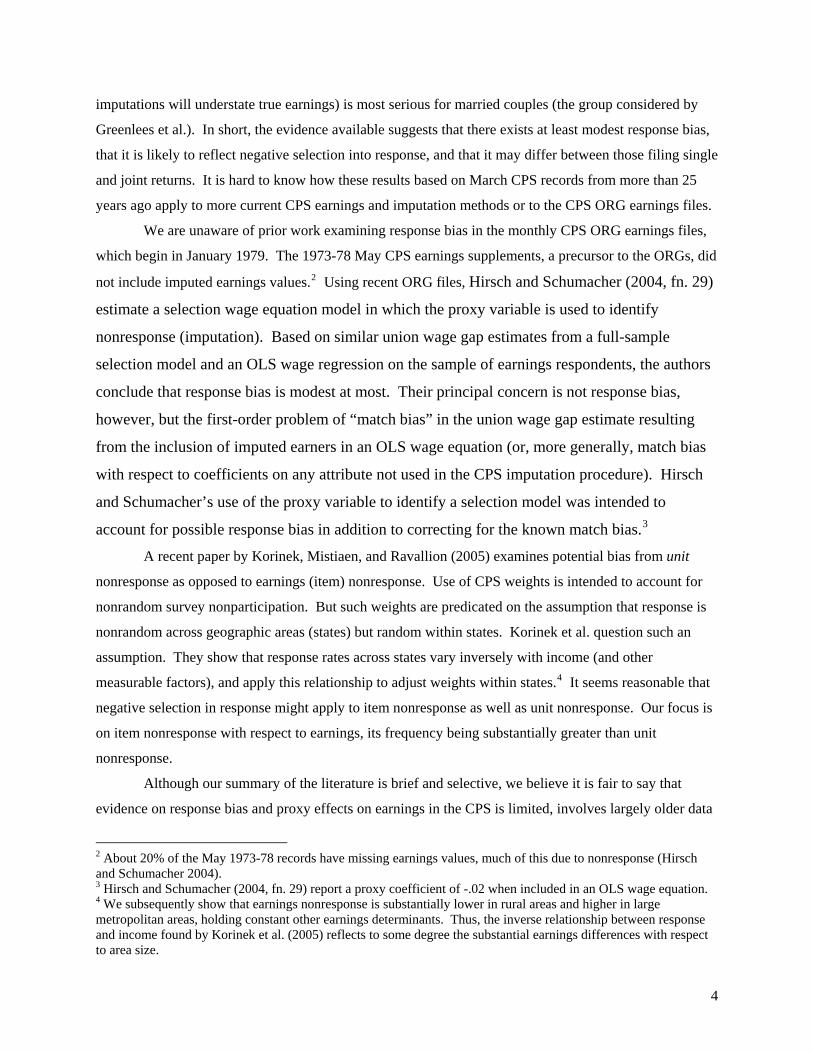
Table 4 presents results from the response probits. We report the marginal effects (evaluated at

the mean of all variables), allowing comparison to tables 1 and 2 and providing some information on the

relative magnitude of these effects. Qualitatively, the results are very comparable across the two samples

and by gender. The marginal effects are larger in magnitude for the ORG than for the March survey, due

largely to the higher nonresponse rate in the ORG. A few variables have different signs in the ORG and

March samples, perhaps due to each model containing unique regressors (e.g., union status is included in

the ORGs; an in-coming rotation group dummy – MIS 1 or 5 – is included in the March).

The information gleaned from table 4, which shows partial effects, is generally similar to that

gleaned from the means in tables 1 and 3. A rundown of results is not warranted. Variables with the

largest marginal effects are Proxy, Age 55+, Married Male, Black, and Asian. All else constant, a proxy

respondent other than a spouse decreases the likelihood of response by about 20%, while a spouse proxy

decreases response only slightly, something under 5%. An interesting difference by gender is that in

ORG, the sensitivity of response to the presence of a proxy, spouse or otherwise, is somewhat greater for

women’s earnings records than for men’s. In the March CPS, exactly the opposite is the case.

Differences by sex, however, are small in both data sets.

The multivariate probit analysis does not change what was found in table 1 for potential

instruments. Proxy respondents are less likely to answer the earnings questions. In the ORG, response

rates are approximately 5 percentage points higher in February and March than in the rest of the year.

And in the ASES data, response rates are about 2 percentage points higher for people in their first of four

months in the survey during each of two consecutive years (rotation groups 1 and 5). The proxy variable

and the interview timing variables (MIS for the March ASES and Feb/March for the ORG) appear to be

potential instruments for selection models.

Response Rates and Predicted Earnings. An additional way in which evidence on nonresponse is

provided is by seeing how nonresponse varies with predicted earnings. Of course, what we would like to

know is how nonresponse varies with actual earnings, but this cannot be observed directly in the CPS for

the 20% (in the ASES) or 30% (in the ORG) who do not report earnings.10 Seeing how response varies

10 The earnings records of nonrespondents include imputed values, but these represent the earnings of respondents with the same mix of imputation match attributes as the nonrespondents and thus add no additional information.

10

with predicted earnings (a weighted mix of earnings attributes) may be suggestive. It tells us how

response varies with measured earnings attributes. If unmeasured skill (or other) attributes are positively

correlated with the measured attributes included in our wage equation, then the response pattern seen with

respect to predicted earnings is likely to reveal the pattern with respect to unmeasured attributes and true

earnings.

Figures 1 and 2 show how nonresponse rates vary with respect to earnings ventiles (one-twentieth

of the distribution) for the ORG and March earnings files, respectively. The figures show nonresponse

for those with predicted earnings in percentiles 0-5, 5-10, 10-15, and so forth. We also separately break

out the 99th percentile.11 The extraordinary thing about Figures 1 and 2 is how little response varies by

predicted earnings. Over much of the earnings distribution, nonresponse rates vary little from the

average. Having said this, there is a clear pattern in both data sets suggesting at least moderated negative

selection into earnings response, although more notably so for men than women. In both data sets,

response rates are highest among those in the top 5% of the wage distribution and, in particular, the top

percentile. For example, in the ASES, the nonresponse rate is 21.8% for the top percentile (18.8% for the

top ventile), compared to mean nonresponse for the entire sample of 18%. Also notable, at least in the

ORG, is a somewhat higher response rate for those with the lowest predicted earnings. Apart from the

bottom tenth and top tenth of the earnings distribution, however, response rates are remarkably similar,

with some hint of slightly declining nonresponse with respect to predicted earnings over the broad middle

of the distribution.

The pattern shown in the figures suggest negative selection into response, more so for men than

women. If an identical pattern holds with respect to actual as well as predicted earnings then it implies

that earnings equations based on respondents (and imputed earners assigned the earnings of respondent

donors) will tend to understate earnings. That being said, the more notable pattern is the rather small

difference in nonresponse with respect to predicted earnings, suggesting that response bias, if it exists, is

likely to be minor or at most quite modest. We turn to this issue below.

Cross Sectional Evidence for Response Selection: Significance versus Importance

In order to investigate the effects of nonresponse, we estimate rich log-linear wage models similar

to those explored in Bollinger and Hirsch (2006). As noted by Bollinger and Hirsch, inclusion of imputed

earners would lead to attenuation in estimated coefficients in many cases. Although some variables are

not significantly affected, non-match imputation attributes (e.g., union status, foreign born) have bias

toward zero of about 25%, while attributes for which there is imperfect matching (e.g., schooling, etc.)

11 Depending on year, about .5% to 1.5% of the ORG sample has earnings that are top-coded. We have yet to examine the incidence of top coded earners in the top percentiles of the predicted earnings distribution.

11

display varied forms of bias. If negative selection into response is also a problem, coefficients would be

biased downward even further. Including the imputed values in a wage equation is not a valid solution

for response bias since the imputations are simply predicted values from the respondents.

Tables 5 and 6 presents log-wage estimates for both the ORG and ASES samples, table 5 for men

and table 6 for women. The first and fourth columns are simply OLS estimates using only respondents

(we do not present OLS estimates of the full sample, given that these are severely biased). The second

and fifth column use both proxy and the interview timing variables (either month or month in sample) as

instruments in the selection equation. Because of concern that proxy is correlated with the wage and is

thus not an ideal instrument, the third and sixth columns use only the month in sample as instruments in

the selection equation. Proxy is such a strong predictor of response that it is natural to consider it as an

instrument, especially given that it should have no direct impact on wages or earnings realized in the labor

market. Proxy may be correlated with the measured wage, however, if proxy respondents report higher or

lower earnings than do self-respondents. We restrict the ORG sample to workers in full-time jobs and the

ASES sample to full-time, full-year workers the previous calendar year. The purpose in this restriction is

to avoid entangling selection into employment and hours with possible selection into response.

We first examine the coefficients on the Mills ratio selection terms in tables 5 and 6, comparing

results for men and women, between the ORG and ASES, and with and without the inclusion of the proxy

variables (both proxy and spouse proxy) as instruments in the selection equation. In table 5, the Mills

ratios for men are negative, highly significant, and quite stable regardless of the inclusion of the proxy

variables as instruments. Based on these selection results, we conclude that men exhibit negative

selection into response.

The Mills ratios for women, as seen in table 6, are more sensitive to the use of the proxy variable

as an instrument. In regressions using the proxy variables as instruments, we obtain significant, negative

coefficients on the Mills ratios using both the ORG and ASES. Absent the use of Proxy (that is, with

only the first or fifth rotation month in sample as an instrument) the coefficient on the selection terms falls

to nearly zero in the ORG. The decline is less sharp using ASES (from -.17 to -.11), but it becomes

statistically insignificant. One possible interpretation of the results for women is that there is little or no

response bias, models using Proxy as an instrument providing misleading results due to a systematic

relationship of earnings with proxy response (evidence examined subsequently). The other possibility is

that the interview timing variables are only weakly related to selection for women. Yet our results in

table 4 seem to discount this possibility. Hence, our conclusion based on results to this point in the paper

is that response bias among full-time women may be weak, certainly not as strong as seen for men.

We next turn to examine the practical importance of selection on estimates of coefficients.

Because of large sample sizes, even trivial differences in coefficients can be statistically significant. We

12

focus on the magnitude of coefficient differences between wage equations with and without an accounting

for selection into response. To examine these differences, we return to tables 5 and 6, which allows us to

compare coefficients from OLS regressions using respondents only (full sample OLS wage equations

suffer from severe match bias due to imputation) and full-sample selection equations. For example,

consider the table 5 results for full time men for the coefficients on elementary education (relative to high

school) estimated by OLS versus results with alternative sample selection corrections for response. The

OLS estimate for the ORG sample is -0.181, while the selection estimates are -0.189 or -0.190. While the

change is statistically significant, the general conclusions one would typically draw are not likely to be

sensitive to this change in magnitude.12 Indeed some coefficients such as the coefficient on foreign-born

in the ORG sample, or the coefficient on Master’s degree in the ASES sample, have a zero change at

three decimal places.

Nearly all the coefficients rise in magnitude moving from OLS with the respondents sample to a

selection model with the full sample, consistent with the coefficient attenuation expected from selection.

But the larger point is that most changes in coefficients are quite minor. For most applications the choice

of approach will have little effect on interpretation of coefficients (other than the intercept). There are,

however, a number of exceptions. Perhaps the clearest examples are the coefficient on Asian, the

selection corrected coefficient being over 50% smaller in magnitude, although the change in log points is

modest. Other notable changes are in the coefficient on Black, Mid-Atlantic, Mountain, and Pacific

regions. Note that variables whose coefficients are most affected by use of a selection model are, not

surprisingly, those for variables highly correlated with rates of earnings nonresponse.

Although response bias appears to have little effect on most wage equation coefficient estimates,

this need not imply selection into response is not an important issue for some applications. Another

approach to assess the impact of the selection correction for response is to predict wages or earnings for

the sample using both the OLS coefficients for respondents and the selection corrected estimates. These

results are seen in Table 7. Using the models in tables 5 and 6 (by gender and for full time workers in the

ORG and full time year round workers in the ASES, and not using Proxy as a selection instrument), we

predict the log wage using first OLS and then the selection model (but not including the selection term in

the prediction). The difference between these two is a measure of the importance of selection to the

model. We find that the difference is (perhaps surprisingly) a sizable -0.09 and -0.12 log points for men

using the ORG and ASES, respectively. That is, negative selection into response among men causes

average earnings to be understated by roughly 10%. Importantly, these differences are produced

12 Bollinger and Hirsch (2006) provide weighted least squares results on the respondent sample using inverse probability weights to account for differences in the probability of response. We suspect that IPW estimates of the respondent sample coefficients would be closer than is OLS to the selection model coefficients, but we have not performed this exercise.

13

primarily by differences in the intercepts and not in slope coefficients, the latter often being the principal

concern of researchers.13 Note as well that our result is similar to the Greenlees et al. and Herriot and

Spiers (1975) studies that used the match March 1973 CPS and 1972 Social Security earnings records.

In sharp contrast to men, for women the difference in the predicted wages from OLS and the

selection model is quite modest, a 1% understatement by OLS using the ORG and a 3% understatement

using ASES. As with men, most of the prediction differences are driven by intercept differences.

In short, our conclusion to this point is that selection into response is negative for men, perhaps

substantially so, while minor among women. In general, regression coefficients (apart from intercepts)

are not particularly sensitive to selection, but coefficients of variables highly correlated with nonresponse

can be affected. We should reiterate a point made earlier. OLS estimates are based on earnings

respondents only. Inclusion of records whose earnings are imputed lead to coefficient match bias of first-

order importance, even when nonresponse is random (Hirsch and Schumacher 2004; Bollinger and Hirsch

2006).

Longitudinal Analysis: Identifying Response Bias as a Fixed Effect?

The selection model approach from the prior section suggests that there exists negative selection

into response among men, but little selection among women. We provide further evidence on possible

response bias by conducting wage change analysis with constructed CPS panels in which each worker is

observed in the same month in consecutive years. Longitudinal analysis allows us to account

(imperfectly) for the worker heterogeneity that is the source of response bias – unmeasured differences in

workers who are likely and not likely to respond to earnings questions. For workers who respond in one

year but not in another year, we can compare their respondent earnings value to the imputed earnings

value in the other year. Imputed values (on average) provide a good measure of the earnings of

respondents (donors) with identical measured attributes, at least those attributes that are included as

Census match criteria. The longitudinal analysis provides two alternative measures of response bias. Let

each person’s reporting status be either R (respondent) or I (imputation) in year 1 and 2. One measure

compares the difference in wage growth for individuals who are R/I versus R/R and the other measure

compares wage growth for those who are I/R versus I/I. If there is negative selection into response, then

imputations should understate actual earnings; hence the first measure should be negative and latter

positive. We would expect these measures to be symmetrical (i.e., have the same absolute value).

13 But not always, as in studies using Oaxaca decomposition, which includes the intercept as part of the unexplained (or discrimination) component. Given our preliminary conclusion that negative selection into response is present and nontrivial for men, but very minor among women, an implication is that the gender wage gap is understated.

14

The key assumption in this analysis is that individuals who fail to respond in one of the two years

are (at least to some extent) similar to nonrespondents, while the imputed values represent the earnings of

respondents with the same measured attributes. If those who are R/I and I/R are just like those who never

respond then the wage change differences should provide a good measure of response bias. If response

“switchers” have unmeasured differences that are somewhere between workers who typically respond and

those who typically refuse to respond, wage change estimates should be qualitatively correct but will

understate the degree of response bias. In subsequent work, we will explore ways to determine whether

R/I and I/R individuals are more similar to R/R or I/I individuals.

Table 8 provides the mean wage changes for the four possible groups, separately for women and

men and for the ORG and ASES panels. Results are cleaner when we control for changes in

characteristics (union status, broad occupation and industry, etc.), but we are uncomfortable presenting

such analysis since inclusion of imputed earners biases coefficient estimates (Bollinger and Hirsch 2006).

Another concern is the appropriate treatment of those with top-coded earnings in one or both years. For

these reasons, these results should be regarded as suggestive and preliminary.

The ORG results are surprisingly clear-cut, with 3% higher wages from respondents than from

the Census imputation, with similar results for women and men and symmetry in the two measures.

Among men, R/I workers displayed a -.031 slower log wage change than did R/R workers, while I/R

workers displayed .034 more wage gain than did I/I workers. For women the equivalent values are -.030

and .041. Assuming that response switchers have unobservables that are somewhere in between those of

those who always and never respond, then the magnitude of response bias exceeds 3%. The ORG results

for men are thus entirely consistent (in direction and magnitude) with our earlier selection results,

reinforcing the conclusion that nonrespondents have higher earnings than do respondents with similar

measured attributes. We obtain similar longitudinal results for women, however, for whom evidence for

negative selection was rather weak in the analysis up to this point.

Evidence from the ASES panels confuses matters further, perhaps due to the smaller size of the

March panels (earnings change data are very noisy), differences in March and ORG imputation methods,

and failure to account for earnings caps in the March surveys. Among men, we observe R/I earnings

growth -.038 slower than for R/R workers, but I/R earnings growth is identical to that for I/I workers. For

women we observe .063 more earnings growth for I/R than for I/I workers, but no difference between R/R

and R/I workers.

In both the ORG and ASES we observe earnings growth differing between always-responders

and always-imputed (R/R and I/I), although nothing in theory tells us that this should be so. This

suggests that other (hopefully measurable) attributes might account for these differences; thus a

multivariate framework seems more appropriate and may provide a more reliable measure of response

15

bias. An additional complicating factor is that the respondent values include not only self-reports but

proxy reports of earnings. In the next section we will examine the relationship between proxy response

and earnings.

Do Proxy and Self Respondents Report Earnings Differently?

To this point our discussion of proxy respondents has focused on its relationship to earnings

nonresponse and imputation. Because individual records based on proxy interviews are substantially less

likely to have earnings reported, use of a proxy provides a potential instrument to identify selection into

response, assuming proxy reports are not correlated with earnings. About half of all CPS records are

based on interviews from proxy rather than self respondents. Thus, the question of whether or not proxy

earnings reports differ from self-reports is important in its own right, independent of the issue of

nonresponse. We explore the issue of proxy response and earnings based on OLS earnings level

equations and using longitudinal analysis in which within-worker proxy wage effects are identified from

workers switching between earnings reports based on self-response and a proxy response. Since changes

in interviewers between one year and the next are likely to be exogenous with respect to wage change,

this approach has appeal. Because over half of all proxy respondents are spouses, we examine separately

spousal and non-spouse proxy effects. As in prior sections, analysis is conducted using both the CPS

ORG and March ASES, with results shown separately for women and men.

Table 9 presents proxy coefficients from OLS earnings level equations. As shown previously

(Hirsch and Schumacher 2004), proxy wage reports are moderately lower than self reports. Using the

ORGs, wages for men based on proxy reports lower by are -.028 than those on self reports; for women the

equivalent estimate is -.019. Using the March CPS, the estimate proxy effect for men is -.027, nearly

identical to that from the ORG, but is tiny for women, being just -.007.14 Given that for men most proxy

reports are provided by women, and for women most proxies are men, it is not surprising that results by

gender can differ.

One of our more interesting findings, to our knowledge not one previously reported, is that the

earnings responses of spousal proxies are substantially different from those of non-spousal proxies.15 As

evident in table 9, earnings reports from non-spousal proxies are substantially lower than self-reports,

whereas spousal reports differ little from self-reports. Among men in the ORGs, non-spouse proxies

report wages -.06 log points lower than self reports, but men whose spouse reports earnings report wages

14 Recall that Angrist and Krueger (1999) concluded that proxy reports of earnings are not substantially different from self repots based on a March CPS sample. 15 In this version of our paper, we lump all non-spousal proxies together and do not report earnings differences within this heterogeneous group.

16

just -.01 less. Using the March CPS, reported earnings for men are a sizable -.09 less when there are non-

spouse proxies. Differences in self and proxy reports are nearly zero (.005) when there is a spouse proxy.

A similar pattern is found for women. In the ORG, non-spouse proxies provide wage reports -.05

log points lower than self reports, but spousal proxies report wages similar to self reports (a coefficient of

.005). Using the March CPS, reported earnings of women are -.05 log points lower with non-spouse

proxies. Women with spouse proxies have reported earnings that are .025 higher than self reports.

In short, standard earnings level equations indicate that proxy reports by non-spouse household

members are strongly correlated with earnings, indicating earnings that are substantively lower than self

reported earnings from otherwise similar workers. Spouse proxies, however, who account for more than

half of all proxy responders, provide earnings reports nearly identical to self reports. An interesting

implication of these findings is that that spouse proxy (but not non-spouse proxy) may provide an

appropriate instrument to account for nonresponse.16 For our discussion here, the question is how best to

interpret the intriguing stylized fact of a large negative non-spousal proxy correlation with earnings.

Why are proxy reports, at least those from non-spouses, correlated with earnings? Is the apparent

proxy effect on earnings really a reporting error producing mismeasured individual earnings? One

possibility is that this is not a reporting problem. Rather, there may be unobserved worker heterogeneity

correlated with the use of a non-spouse proxy – workers whose earnings are reported by a proxy

household member other than a spouse having low unmeasured “skills” (i.e., any earnings related

characteristics) as compared to earners who self-report or who rely on spouse proxies. Moreover,

heterogeneity showing up in the proxy coefficients may reflect nonignorable response bias, given the

strong correlation between proxy reports and earnings nonresponse. Longitudinal analysis, which nets

out heterogeneity as a worker fixed effect, provides a straightforward way to examine this possibility.

Table 10 provides longitudinal results using the CPS panels, which identifies the effects of proxy

reports based on the difference in earnings growth between those switching between proxy and self

reports and those who do not change proxy status. We focus initially on the ORG panels, which have

larger total sample sizes, large samples of switchers, and a cleaner definition of earnings (the wage on the

principal job last week versus earnings in all wage and salary jobs in the previous year). Non-spouse

wage effects in the panel analysis are considerably lower than in the wage level equation. Men switching

from a self-report in year 1 to a non-spouse proxy report in year 2 display -.014 slower wage growth than

those with self-reports in both years. Men switching from a non-spouse proxy in year 1 to a self-report in

year 2 display .019 faster wage growth than those with non-spouse proxy reports in both years. These

longitudinal estimates of a 1-2% non-spouse proxy effect can be compared to the large -.060 effect

reported in the wage level equation. Those switching from a self-report to a spouse report display -.014 16 Response bias estimates using non-spouse proxy as an instrument are not included in this version of the paper.

17

lower wage growth, while those switching in the opposite direction display .008 faster growth. In short,

the ORG panel results for men find that proxy reports are only modestly lower than self reports, with

roughly similar magnitudes for both non-spouse and spouse proxies. These very modest proxy effects are

in line with the estimates found by Mellow and Sider (1983) in their validation study using a special

January 1977 CPS supplement.

Turning to the ORG panel for women, one continues to find that proxy reports are slightly lower

than self reports, again with no evidence that of stronger effects for non-spouse than spouse proxies.

Women switching from a self-report in year 1 to a non-spouse proxy report in year 2 display -.014 slower

wage growth than those self-reporting in both years, as compared to the -.050 reported in the wage level

equation seen in table 9. Those switching from a self-report to a spouse report also display -.014 slower

wage growth. For both women and men, much of the large proxy effect found for non-spouses in the

wage level equations is due to worker heterogeneity – lower earnings attributes (unmeasured) for workers

who have non-spouse than spouse proxies. There remains a “real” difference in proxy and self reports of

earnings, but they appear to be small, on the order of 1-2%. That being said, for the standard wage level

equations seen throughout the labor economics literature, there exists considerable unmeasured worker

heterogeneity, including that correlated with nonresponse and the presence of a non-spouse proxy.

March CPS panel results tend to be less precise than the ORG panels, but provide a generally

similar story, with non-spouse proxy effects smaller in the panel than in the earnings level equations.

Men switching from a self-report in year 1 to a non-spouse proxy report in year 2 display higher rather

than lower earnings growth (by .017) than those self-reporting in both years, while those switching from a

non-spouse to a self-report display .067 faster earnings growth.17 These effects can be compared to the

large -.090 non-spouse proxy effect found in the March earnings level equation. Among men with spouse

proxies, those switching from self to spouse reports display -.012 slower earnings growth, while those

switching in the opposite direction display .019 earnings gain. These latter estimates are consistent with

the 1-2% proxy wage effects seen in the ORG panels.

Among women in the March CPS, those switching from a self-report in year 1 to a non-spouse

proxy report in year 2 display -.035 lower earnings growth than those self-reporting in both years, while

those switching from a non-spouse to a self-report display .041 faster earnings growth. These estimates

are only modestly lower than the -.05 non-spouse proxy effect found in the March earnings level

equation. Women switching to a spouse proxy from a self report, earnings growth is nearly equivalent

(.005 higher), as is the case for those switching in the opposite direction (-.014 lower earnings growth).

17 Note that all of the longitudinal estimates of wage change are relative to the wage growth of a control group or base category. Unusual wage growth for the control group will thus be reflected in the parameter estimates.

18

The results from the March panel indicate that spousal proxy effects on reported earnings are effectively

zero, but that non-spousal reports have a modest but real negative effect.

Taken as a whole, the panel evidence reveals that even after accounting for worker heterogeneity,

there exist small to modest effects of proxy respondents, with proxy reports tending to provide lower

reports of earnings than self reports. Lower reporting is less evident for spouse than for non-spouse proxy

reports in the March panels, but in the larger ORG panels we observe no difference. For both data sets, it

is reasonable to conclude that both spouse and non-spouse proxy effects on earnings are quite modest.

Absent an accounting for worker heterogeneity (worker fixed effects), proxy reports are of far greater

concern. In standard wage level equations, non-spouse proxy reports, but not spouse proxy reports, are

substantially lower than self reports. This large difference in spouse and non-spouse reporting, however,

is the result of unobserved worker heterogeneity that is netted out in the panel analysis.

Finally, note that the results reported in this section include only earnings respondents and do not

deal directly with selection into response. We have estimated full-sample selection equations that include

control for selection into response. As seen previously, selection into response is an issue in wage level

equations, although far more so for men than for women. Indeed part of what shows up in table 9 as an

apparent reporting effect of proxy respondents is in fact the result of selection. Using selection wage

level equations, results for non-spouse proxies are greatly diminished and look more like our wage change

than wage level results. We have seen that proxy reporting effects are diminished greatly in the

longitudinal analysis. Part of what we have been calling worker heterogeneity is unobserved differences

with respect to selection into response. When we estimate full-sample selectivity adjusted wage change

equations (not shown), we find no evidence for selection (response bias), as evident by the Mills ratios.

Selection effects are largely worker fixed effects that can be eliminated in the CPS panels.

Conclusions

Nonresponse (accompanied by earnings imputation) and proxy respondents are frequently seen in

household surveys, most notably in the CPS. We examine the issue of response bias and proxy

respondents using the CPS ORG earnings files and the March CPS ASES files. Although labor

economists typically include imputed earners and proxy respondents in empirical studies, recent research

has shown that inclusion of imputed earners in wage studies is problematic (Hirsch and Schumacher

2004; Bollinger and Hirsch 2006). Coefficients on attributes not included as Census imputation match

criteria are severely attenuated, by roughly 25% or close to the percentage of imputed earners. For

coefficients on attributes where the imputation match is imperfect, severe biases can also arise.

Accounting for this bias by throwing out imputations provides a relatively simple fix for the first-order

distortions resulting from match bias. But this and other approaches to correct for match bias (see

19

Bollinger and Hirsch 2006) rest on the important assumption that nonrespondents are conditional missing

at random (nonignorable response bias). This paper explores that question, along with the effect of proxy

earnings reports, given that proxy responses are highly correlated with earnings nonresponse .

Using selection wage equations in which selection is identified by measures on the timing of the

surveys and (in some specifications) proxy respondents, we conclude that that there is negative selection

into response among men. Response bias is far less evident among women. These conclusions match

what is visually evident from descriptive data on nonresponse by percentiles in the predicted earnings

distributions and what has been previously concluded in older validation studies discussed in the text.

Longitudinal analysis is then used to identify response bias based on a comparison of workers’ self

reported earnings with those same workers’ imputed value in the previous or subsequent year. The

imputed values on average measure the earnings of respondents (earnings donors) with identical

measured attributed. Here evidence is that for both men and women, imputations moderately understate

true earnings. This is further support for there being negative selection into response, although why we

find roughly similar effects here for women and men, but not using selection models, is not clear.

Finally, we examine the effect of proxy reports on earnings, based primarily on samples of

earnings respondents. In a standard cross section earnings equations, proxy reports are about 2-3% lower

than self-reports, as has been previously reported in the literature (Hirsch and Schumacher 2004). What

these results mask is a substantive difference between spouse and non-spouse proxies. For both men and

women, in the CPS and ASES, non-spouse proxies report earnings substantially lower than self reports,

whereas spouse proxy reports are very close to self reports. Longitudinal analysis reveals that the non-

spouse reporting effects are not due to reporting error but to unobserved heterogeneity, including that

associated with response bias (since proxy is a strong correlate of response). Response bias appears to be

largely a fixed effect that nets out in the wage and earnings change equations. Based on the longitudinal

analysis, proxy effects on reported earnings tend to be negative, small or moderate in size (1-2%), and not

greatly different for spouse and non-spouse proxies. The “problem” is not the use by Census of proxy

respondents, who provide reasonably accurate reports on earnings, but substantial worker heterogeneity

correlated with both the proxy variable and with nonresponse. It is these forms of worker heterogeneity

about which labor economists need to be concerned.

20

References Angrist, Joshua D. and Alan B. Krueger. “Empirical Strategies in Labor Economics,” in Handbook of

Labor Economics 3A, edited by Orley C. Ashenfelter and David Card. Amsterdam: Elsevier, 1999. Bollinger, Christopher R. and Barry T. Hirsch. “Match Bias from Earnings Imputation in the Current

Population Survey: The Case of Imperfect Matching,” Journal of Labor Economics 24 (July 2006): 483-519.

Bound, John and Alan B. Krueger. “The Extent of Measurement Error in Longitudinal Earnings Data: Do

Two Wrongs Make a Right?” Journal of Labor Economics 9 (January 1991): 1-24. David, Martin, Roderick J. A. Little, Michael E. Samuhel, and Robert K. Triest. “Alternative Methods for

CPS Income Imputation,” Journal of the American Statistical Association 81 (March 1986): 29-41. Greenlees, John, William Reece, and Kimberly Zieschang. “Imputation of Missing Values when the

Probability of Response Depends on the Variable Being Imputed,” Journal of the American Statistical Association 77 (June 1982): 251-61.

Heckman, James J. and Paul A. LaFontaine. "Bias Corrected Estimates of GED Returns," Journal of

Labor Economics 24 (July 2006): 661-700. Herriot, R. A. and E. F. Spiers. “Measuring the Impact on Income Statistics of Reporting Differences

between the Current Population Survey and Administrative Sources,” Proceedings, American Statistical Association Social Statistics Section (1975): 147-58.

Hirsch, Barry T. and Edward J. Schumacher. "Match Bias in Wage Gap Estimates Due to Earnings

Imputation," Journal of Labor Economics 22 (July 2004): 689-722. Korinek, Anton, Johan A. Mistiaen, and Martin Ravallion. “An Econometric Method of Correcting for

Unit Nonresponse Bias in Surveys,” World Bank Policy Research Working Paper 3711 (September 2005).

Lemieux, Thomas. “Increasing Residual Wage Inequality: Composition Effects, Noisy Data, or Rising

Demand for Skill,” American Economic Review 96 (June 2006): 461-98. Lillard, Lee, James P. Smith, and Finis Welch. “What Do We Really Know about Wages? The

Importance of Nonreporting and Census Imputation,” Journal of Political Economy 94 (June 1986): 489-506.

Mellow, Wesley and Hal Sider. “Accuracy of Response in Labor Market Surveys: Evidence and

Implications,” Journal of Labor Economics 1 (October 1983): 331-44.

21

Figure 1

Percent Imputed by Predicted Wage Ventile, CPS-ORG, 1998-2006

15

20

25

30

35

40

0 5 10 15 20 25 30 35 40 45 50 55 60 65 70 75 80 85 90 95 99

Percentile of Predicted Wage

Perc

ent I

mpu

ted

Full SampleMenWomen

Figure 2

Percent Imputed by Predicted Earnings Ventile, March CPS ASES, 1998-2006

10

12

14

16

18

20

22

24

5 10 15 20 25 30 35 40 45 50 55 60 65 70 75 80 85 90 95 100 99

Predicted Ventile

Perc

ent I

mpu

ted

All WorkersMale WorkersFemale Workers

Table 1: Sample Sizes and Percent Earnings Nonresponse CPS ORG Sample March CPS ASES Sample

Year N %Non-Respondent N %Non-Respondent1998 150,621 23.4 62,227 14.7 1999 156,991 27.5 63,119 16.3 2000 158,868 29.7 64,763 15.9 2001 168,962 30.8 62,534 18.6 2002 181,309 30.2 102,896 18.6 2003 178,163 31.8 100,657 19.4 2004 175,195 31.5 98,543 19.4 2005 176,401 30.8 96,844 19.3 2006 176,048 30.9 96,371 17.3

Self Report 766,623 24.1 331,840 14.1 Any Proxy Report* 756,425 35.4 353,887 22.2 Spouse Proxy* 422,796 30.1 251,920 16.9 MIS 1 or 5 n.a n.a 189,762 16.4 MIS 2-4, or 6-8 n.a n.a 578,288 18.5 February 126,579 26.3 n.a. n.a. March 125,231 25.4 n.a. n.a. Total %Imputed 1,523,048 29.6 747,954 18.0

*not available for one year of the March CPS

Table 2: Proxy Respondents by Gender and Marital Status

ORG Sample March ASES Sample All Men Women All Men Women Any Proxy 50.3% 58.9% 41.5% 51.6% 60.7% 42.8% Spouse Proxy 27.8% 34.6% 20.7% 27.9% 34.3% 21.2% % of All Proxies who are Spouse

55.2% 58.8% 49.7% 54.0% 57.1% 49.5%

Table 3: Means by Response Status ORG Sample ASES Respondent Non-Respondents RespondentsNon-Respondents Age 39.30 40.75 38.75 39.42 Under age 25 0.15 0.14 0.17 0.19 Prime Age 0.72 0.70 0.78 0.74 Age 55 and over 0.13 0.16 0.12 0.15 Elementary School 0.03 0.03 0.04 0.04 H.S. Dropout 0.09 0.08 0.11 0.11 H.S. Graduate 0.30 0.34 0.30 0.32 Some College 0.20 0.19 0.20 0.20 Associates Degree 0.10 0.09 0.09 0.08 Baccalaureate Degree 0.19 0.18 0.18 0.17 Master's Degree 0.07 0.06 0.06 0.05 Professional Degree 0.01 0.01 0.01 0.01 Ph.D. 0.01 0.01 0.01 0.01 Female 0.50 0.48 0.50 0.48 White 0.77 0.72 0.70 0.66 Black 0.08 0.12 0.09 0.13 Asian 0.03 0.05 0.04 0.05 Hispanic 0.10 0.10 0.15 0.15 Single Male 0.14 0.16 0.14 0.18 Single Female 0.13 0.13 0.13 0.15 Married Male 0.30 0.30 0.30 0.28 Married Female 0.27 0.25 0.27 0.24 Previously Married Male 0.06 0.07 0.06 0.06 Previously Married Female 0.10 0.10 0.10 0.10 Non-MSA 0.28 0.23 0.27 0.23 MSA under 250K 0.07 0.06 0.07 0.06 MSA 250K to 500K 0.09 0.08 0.09 0.08 MSA 500K to 1M 0.11 0.11 0.11 0.11 MSA 1M to 2.5M 0.17 0.17 0.17 0.17 MSA 2.5M to 5M 0.09 0.09 0.09 0.08 MSA 5M + 0.20 0.26 0.21 0.27 Northeast 0.10 0.10 0.09 0.11 Mid-Atlantic 0.10 0.14 0.11 0.14 East North Central 0.13 0.15 0.13 0.15 West North Central 0.13 0.09 0.11 0.09 South Atlantic 0.16 0.18 0.16 0.18 East South Central 0.05 0.05 0.05 0.05 West South Central 0.08 0.08 0.09 0.07 Mountain 0.13 0.08 0.12 0.09 Pacific 0.13 0.12 0.14 0.14 Weekly Earnings (in 2006$) $752.91 Annual Earnings (in 1980 $) $36,766 Sample Size 1,069,829 453,219 613,501 134,453

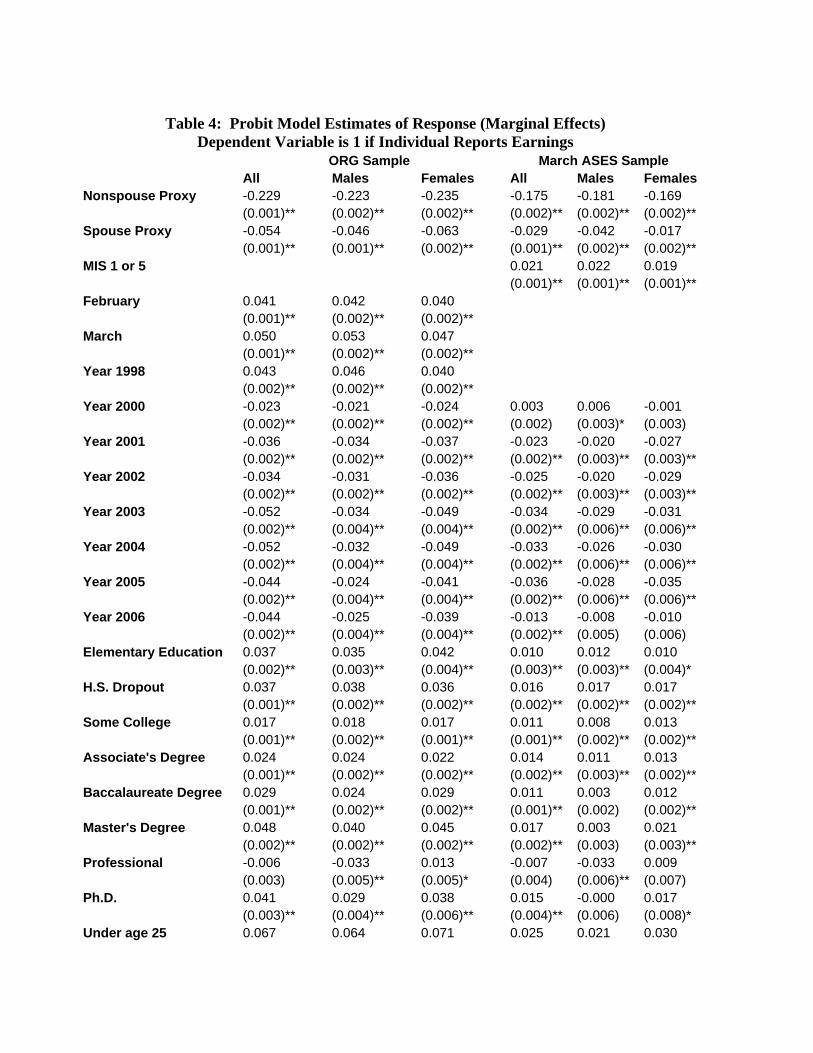
Table 4: Probit Model Estimates of Response (Marginal Effects)

Dependent Variable is 1 if Individual Reports Earnings ORG Sample March ASES Sample All Males Females All Males FemalesNonspouse Proxy -0.229 -0.223 -0.235 -0.175 -0.181 -0.169 (0.001)** (0.002)** (0.002)** (0.002)** (0.002)** (0.002)** Spouse Proxy -0.054 -0.046 -0.063 -0.029 -0.042 -0.017 (0.001)** (0.001)** (0.002)** (0.001)** (0.002)** (0.002)** MIS 1 or 5 0.021 0.022 0.019 (0.001)** (0.001)** (0.001)** February 0.041 0.042 0.040 (0.001)** (0.002)** (0.002)** March 0.050 0.053 0.047 (0.001)** (0.002)** (0.002)** Year 1998 0.043 0.046 0.040 (0.002)** (0.002)** (0.002)** Year 2000 -0.023 -0.021 -0.024 0.003 0.006 -0.001 (0.002)** (0.002)** (0.002)** (0.002) (0.003)* (0.003) Year 2001 -0.036 -0.034 -0.037 -0.023 -0.020 -0.027 (0.002)** (0.002)** (0.002)** (0.002)** (0.003)** (0.003)** Year 2002 -0.034 -0.031 -0.036 -0.025 -0.020 -0.029 (0.002)** (0.002)** (0.002)** (0.002)** (0.003)** (0.003)** Year 2003 -0.052 -0.034 -0.049 -0.034 -0.029 -0.031 (0.002)** (0.004)** (0.004)** (0.002)** (0.006)** (0.006)** Year 2004 -0.052 -0.032 -0.049 -0.033 -0.026 -0.030 (0.002)** (0.004)** (0.004)** (0.002)** (0.006)** (0.006)** Year 2005 -0.044 -0.024 -0.041 -0.036 -0.028 -0.035 (0.002)** (0.004)** (0.004)** (0.002)** (0.006)** (0.006)** Year 2006 -0.044 -0.025 -0.039 -0.013 -0.008 -0.010 (0.002)** (0.004)** (0.004)** (0.002)** (0.005) (0.006) Elementary Education 0.037 0.035 0.042 0.010 0.012 0.010 (0.002)** (0.003)** (0.004)** (0.003)** (0.003)** (0.004)* H.S. Dropout 0.037 0.038 0.036 0.016 0.017 0.017 (0.001)** (0.002)** (0.002)** (0.002)** (0.002)** (0.002)** Some College 0.017 0.018 0.017 0.011 0.008 0.013 (0.001)** (0.002)** (0.001)** (0.001)** (0.002)** (0.002)** Associate's Degree 0.024 0.024 0.022 0.014 0.011 0.013 (0.001)** (0.002)** (0.002)** (0.002)** (0.003)** (0.002)** Baccalaureate Degree 0.029 0.024 0.029 0.011 0.003 0.012 (0.001)** (0.002)** (0.002)** (0.001)** (0.002) (0.002)** Master's Degree 0.048 0.040 0.045 0.017 0.003 0.021 (0.002)** (0.002)** (0.002)** (0.002)** (0.003) (0.003)** Professional -0.006 -0.033 0.013 -0.007 -0.033 0.009 (0.003) (0.005)** (0.005)* (0.004) (0.006)** (0.007) Ph.D. 0.041 0.029 0.038 0.015 -0.000 0.017 (0.003)** (0.004)** (0.006)** (0.004)** (0.006) (0.008)* Under age 25 0.067 0.064 0.071 0.025 0.021 0.030

(0.001)** (0.002)** (0.002)** (0.002)** (0.002)** (0.002)** Over age 55 -0.073 -0.081 -0.062 -0.055 -0.058 -0.052 (0.001)** (0.002)** (0.002)** (0.002)** (0.002)** (0.002)** Married Male -0.013 -0.012 -0.011 -0.007 (0.002)** (0.002)** (0.002)** (0.002)** Married Female -0.024 -0.024 -0.018 -0.024 (0.001)** (0.002)** (0.002)** (0.002)** Previously Married Male -0.004 -0.002 0.004 0.002 (0.002)* (0.002) (0.002) (0.003) Previously Married Female 0.002 0.001 -0.000 (0.002) (0.002) (0.002) Single Female 0.003 0.003 0.004 (0.001) (0.002) (0.002)* Black -0.082 -0.081 -0.085 -0.043 -0.042 -0.045 (0.001)** (0.002)** (0.002)** (0.002)** (0.003)** (0.002)** Asian -0.054 -0.059 -0.053 -0.035 -0.036 -0.038 (0.002)** (0.003)** (0.003)** (0.003)** (0.004)** (0.004)** Other 0.005 0.013 -0.002 -0.004 -0.006 -0.002 (0.003) (0.004)** (0.004) (0.003) (0.005) (0.005) Hispanic 0.026 0.029 0.022 -0.002 0.001 -0.004 (0.001)** (0.002)** (0.002)** (0.002) (0.002) (0.002) Foreign 0.007 0.007 0.010 0.012 0.009 0.017 (0.001)** (0.002)** (0.002)** (0.002)** (0.002)** (0.002)** Veteran 0.005 0.004 0.035 (0.001)** (0.002)** (0.005)** Central City -0.002 -0.004 0.000 0.001 -0.001 0.003 (0.002) (0.002) (0.002) (0.001) (0.002) (0.002) Metro under 250M 0.010 0.013 0.010 0.012 0.011 0.012 (0.002)** (0.002)** (0.002)** (0.002)** (0.003)** (0.003)** Metro 250K-500K -0.015 -0.016 -0.013 0.005 0.003 0.007 (0.002)** (0.002)** (0.002)** (0.002)** (0.003) (0.003)** Metro 500K-1M -0.022 -0.021 -0.020 -0.014 -0.015 -0.014 (0.001)** (0.002)** (0.002)** (0.002)** (0.003)** (0.003)** Metro 1M-2.5M -0.024 -0.022 -0.023 -0.004 -0.005 -0.004 (0.001)** (0.002)** (0.002)** (0.002)** (0.002)* (0.002) Metro 2.5M - 5M -0.035 -0.033 -0.033 -0.004 -0.006 -0.002 (0.002)** (0.002)** (0.002)** (0.002)* (0.003)* (0.003) Metro 5M + -0.063 -0.061 -0.061 -0.029 -0.030 -0.028 (0.001)** (0.002)** (0.002)** (0.002)** (0.002)** (0.002)** Mid Atlantic -0.032 -0.032 -0.029 -0.001 -0.004 0.002 (0.002)** (0.002)** (0.002)** (0.002) (0.003) (0.003) East North Central 0.000 -0.002 0.000 0.007 0.005 0.008 (0.002) (0.002) (0.002) (0.002)** (0.003) (0.003)** West North Central 0.069 0.071 0.069 0.044 0.044 0.044 (0.002)** (0.002)** (0.002)** (0.002)** (0.003)** (0.003)** South Atlantic -0.005 -0.002 -0.004 0.010 0.010 0.011 (0.002)** (0.002) (0.002) (0.002)** (0.003)** (0.003)**

East South Central -0.014 -0.016 -0.012 0.019 0.017 0.022 (0.002)** (0.003)** (0.003)** (0.002)** (0.004)** (0.003)** West South Central 0.021 0.026 0.020 0.038 0.039 0.039 (0.002)** (0.003)** (0.003)** (0.002)** (0.003)** (0.003)** Mountain 0.080 0.089 0.076 0.060 0.063 0.061 (0.002)** (0.002)** (0.002)** (0.002)** (0.002)** (0.002)** Pacific 0.037 0.041 0.036 0.035 0.036 0.036 (0.002)** (0.002)** (0.002)** (0.002)** (0.003)** (0.003)** Federal Government 0.021 0.000 0.018 0.022 0.017 0.025 (0.002)** (0.003) (0.004)** (0.003)** (0.004)** (0.004)** State Government 0.028 0.018 0.016 0.017 0.022 0.007 (0.002)** (0.003)** (0.003)** (0.002)** (0.003)** (0.003)* Local Government 0.027 0.011 0.020 0.021 0.020 0.017 (0.001)** (0.003)** (0.003)** (0.002)** (0.003)** (0.002)** Part Time, Full Year -0.000 0.003 0.003 (0.002) (0.003) (0.002) Full Time, Part Year 0.036 0.038 0.037 (0.001)** (0.002)** (0.002)** Part Time, Part Year 0.047 0.051 0.049 (0.001)** (0.002)** (0.002)** Part Time 0.055 0.062 0.060 (0.001)** (0.002)** (0.001)** Observations 1,523,048 774,678 748,370 683,218 345,777 337,441

Table 5: Wage Equation Estimates, Full Time (Full Year) Men ORG Sample March ASES Sample

OLS

2-Step with Proxy

2-Step w/o Proxy OLS

2-Step with Proxy

2-Step w/o Proxy

Elementary School -0.181 -0.189 -0.190 -0.235 -0.235 -0.240 (0.003)** (0.004)** (0.004)** (0.006)** (0.007)** (0.007)** Grade 9 -0.146 -0.156 -0.157 -0.208 -0.215 -0.215 (0.004)** (0.005)** (0.005)** (0.009)** (0.009)** (0.009)** Grade 10 -0.121 -0.129 -0.130 -0.175 -0.172 -0.176 (0.004)** (0.005)** (0.005)** (0.009)** (0.009)** (0.009)** Grade 11 -0.098 -0.104 -0.105 -0.154 -0.156 -0.154 (0.003)** (0.004)** (0.004)** (0.007)** (0.008)** (0.008)** Grade 11+ -0.082 -0.080 -0.081 -0.125 -0.125 -0.119 (0.005)** (0.006)** (0.006)** (0.010)** (0.011)** (0.010)** Some College 0.088 0.082 0.082 0.099 0.094 0.092 (0.002)** (0.002)** (0.002)** (0.003)** (0.004)** (0.004)** Associates Degree 0.128 0.121 0.121 0.146 0.142 0.137 (0.002)** (0.002)** (0.003)** (0.004)** (0.005)** (0.005)** Baccalaureate Degree 0.300 0.294 0.294 0.334 0.335 0.331 (0.002)** (0.002)** (0.002)** (0.004)** (0.004)** (0.004)** Masters Degree 0.417 0.407 0.407 0.489 0.489 0.487 (0.003)** (0.003)** (0.003)** (0.006)** (0.006)** (0.006)** Professional Degree 0.743 0.752 0.751 0.951 0.977 0.973 (0.008)** (0.005)** (0.006)** (0.014)** (0.010)** (0.010)** Ph.D. 0.646 0.639 0.638 0.757 0.765 0.762 (0.006)** (0.005)** (0.005)** (0.011)** (0.010)** (0.010)** Experience 0.045 0.043 0.043 0.067 0.062 0.060 (0.001)** (0.001)** (0.001)** (0.002)** (0.002)** (0.002)** Experience-squared (00's) -0.165 -0.150 -0.151 -0.263 -0.229 -0.217 (0.006)** (0.006)** (0.006)** (0.012)** (0.011)** (0.013)** Experience - Cubed (000's) 0.028 0.024 0.024 0.046 0.039 0.036 (0.002)** (0.002)** (0.002)** (0.003)** (0.003)** (0.003)** Experience - quartic (0000's) -0.002 -0.002 -0.002 -0.003 -0.003 -0.002 (0.000)** (0.000)** (0.000)** (0.000)** (0.000)** (0.000)** Married Male 0.132 0.118 0.115 0.189 0.166 0.156 (0.002)** (0.002)** (0.003)** (0.003)** (0.004)** (0.006)** Previously Married Male 0.037 0.025 0.025 0.070 0.050 0.048 (0.002)** (0.002)** (0.003)** (0.004)** (0.005)** (0.006)** Black -0.147 -0.127 -0.126 -0.153 -0.136 -0.130 (0.003)** (0.003)** (0.004)** (0.004)** (0.005)** (0.006)** Asian -0.029 -0.012 -0.010 -0.036 -0.017 -0.011 (0.004)** (0.004)** (0.005)* (0.007)** (0.007)* (0.008) Other -0.061 -0.062 -0.061 -0.082 -0.078 -0.077 (0.005)** (0.005)** (0.005)** (0.009)** (0.009)** (0.009)** Hispanic -0.134 -0.138 -0.138 -0.132 -0.132 -0.131 (0.003)** (0.003)** (0.003)** (0.004)** (0.004)** (0.004)** Foreign -0.136 -0.136 -0.136 -0.156 -0.158 -0.159 (0.003)** (0.003)** (0.003)** (0.004)** (0.004)** (0.004)**

Central City -0.050 -0.051 -0.051 -0.048 -0.051 -0.051 (0.003)** (0.003)** (0.003)** (0.003)** (0.003)** (0.003)** Metro under 250M 0.066 0.063 0.063 0.072 0.067 0.064 (0.002)** (0.003)** (0.003)** (0.004)** (0.005)** (0.005)** Metro 250K-500K 0.087 0.091 0.091 0.101 0.102 0.100 (0.002)** (0.003)** (0.003)** (0.004)** (0.005)** (0.005)** Metro 500K-1M 0.119 0.125 0.125 0.136 0.142 0.145 (0.002)** (0.002)** (0.002)** (0.004)** (0.004)** (0.005)** Metro 1M-2.5M 0.152 0.158 0.159 0.159 0.164 0.164 (0.002)** (0.002)** (0.002)** (0.004)** (0.004)** (0.004)** Metro 2.5M - 5M 0.249 0.258 0.258 0.226 0.233 0.232 (0.003)** (0.003)** (0.003)** (0.005)** (0.005)** (0.005)** Metro 5M + 0.251 0.268 0.268 0.247 0.265 0.267 (0.002)** (0.002)** (0.003)** (0.004)** (0.004)** (0.005)** Mid Atlantic -0.033 -0.023 -0.023 -0.009 -0.007 -0.003 (0.003)** (0.003)** (0.003)** (0.005) (0.006) (0.005) East North Central -0.034 -0.033 -0.034 -0.019 -0.024 -0.023 (0.003)** (0.003)** (0.003)** (0.005)** (0.005)** (0.005)** West North Central -0.080 -0.099 -0.100 -0.075 -0.100 -0.107 (0.003)** (0.003)** (0.004)** (0.005)** (0.006)** (0.008)** South Atlantic -0.050 -0.050 -0.051 -0.056 -0.061 -0.063 (0.003)** (0.003)** (0.003)** (0.005)** (0.005)** (0.005)** East South Central -0.080 -0.076 -0.077 -0.070 -0.076 -0.078 (0.003)** (0.004)** (0.004)** (0.006)** (0.007)** (0.007)** West South Central -0.105 -0.113 -0.114 -0.087 -0.107 -0.112 (0.003)** (0.003)** (0.003)** (0.005)** (0.006)** (0.007)** Mountain -0.020 -0.044 -0.045 -0.030 -0.061 -0.070 (0.003)** (0.003)** (0.004)** (0.005)** (0.006)** (0.008)** Pacific 0.029 0.018 0.018 0.006 -0.009 -0.014 (0.003)** (0.003)** (0.003)** (0.005) (0.005) (0.006)* Federal Government 0.046 0.044 0.045 0.031 0.022 0.015 (0.003)** (0.004)** (0.004)** (0.005)** (0.007)** (0.007)* State Government -0.204 -0.208 -0.207 -0.142 -0.153 -0.157 (0.003)** (0.004)** (0.004)** (0.005)** (0.006)** (0.007)** Local Government -0.179 -0.180 -0.180 -0.061 -0.071 -0.075 (0.003)** (0.003)** (0.003)** (0.004)** (0.005)** (0.006)** Union Member 0.178 0.170 0.170 (0.002)** (0.002)** (0.002)** Mills Ratio -0.183 -0.180 -0.309 -0.381 (0.006)** (0.022)** (0.013)** (0.064)** Constant 2.503 2.580 2.581 9.443 9.571 9.606 (0.005)** (0.006)** (0.011)** (0.010)** (0.012)** (0.029)** Robust standard errors in parentheses 693452 276115 * significant at 5%; ** significant at 1% Industry, Occupation and Year Dummy Variables Included in Specifications

Table 6: Wage Equation Estimates, Full Time (Full Year) Women ORG Sample March ASEC Sample

OLS

2_Step with Proxy

2-Step w/o Proxy OLS

2-Step with Proxy

2-Step w/o Proxy

Elementary School -0.190 -0.198 -0.192 -0.206 -0.201 -0.207 (0.004)** (0.005)** (0.005)** (0.009)** (0.009)** (0.008)** Grade 9 -0.163 -0.169 -0.164 -0.189 -0.189 -0.191 (0.005)** (0.006)** (0.007)** (0.012)** (0.012)** (0.012)** Grade 10 -0.148 -0.153 -0.149 -0.182 -0.185 -0.184 (0.005)** (0.005)** (0.005)** (0.010)** (0.011)** (0.010)** Grade 11 -0.118 -0.122 -0.119 -0.157 -0.161 -0.160 (0.004)** (0.005)** (0.005)** (0.009)** (0.009)** (0.009)** Grade 11+ -0.083 -0.082 -0.082 -0.094 -0.101 -0.093 (0.006)** (0.007)** (0.007)** (0.014)** (0.013)** (0.012)** Some College 0.093 0.089 0.092 0.098 0.095 0.096 (0.002)** (0.002)** (0.002)** (0.003)** (0.004)** (0.004)** Associates Degree 0.170 0.165 0.169 0.185 0.181 0.182 (0.002)** (0.002)** (0.002)** (0.004)** (0.004)** (0.005)** Baccalaureate Degree 0.328 0.323 0.327 0.389 0.388 0.386 (0.002)** (0.002)** (0.002)** (0.004)** (0.004)** (0.004)** Masters Degree 0.490 0.482 0.488 0.581 0.580 0.577 (0.003)** (0.003)** (0.003)** (0.005)** (0.006)** (0.006)** Professional Degree 0.740 0.736 0.739 0.888 0.888 0.886 (0.009)** (0.006)** (0.006)** (0.017)** (0.012)** (0.011)** Ph.D. 0.710 0.701 0.708 0.856 0.855 0.852 (0.008)** (0.007)** (0.007)** (0.016)** (0.013)** (0.013)** Experience 0.044 0.043 0.044 0.062 0.059 0.061 (0.001)** (0.001)** (0.001)** (0.002)** (0.002)** (0.002)** Experience-squared (00's) -0.196 -0.186 -0.194 -0.281 -0.260 -0.269 (0.005)** (0.005)** (0.006)** (0.012)** (0.011)** (0.012)** Experience - Cubed (000's) 0.039 0.036 0.039 0.056 0.051 0.054 (0.002)** (0.001)** (0.002)** (0.003)** (0.003)** (0.003)** Experience - quartic (0000's) -0.003 -0.003 -0.003 -0.004 -0.004 -0.004 (0.000)** (0.000)** (0.000)** (0.000)** (0.000)** (0.000)** Married Female 0.029 0.025 0.028 0.036 0.030 0.031 (0.002)** (0.002)** (0.002)** (0.003)** (0.004)** (0.004)** Previously Married Female 0.004 -0.003 0.003 0.017 0.008 0.011 (0.002)* (0.002) (0.003) (0.004)** (0.004) (0.005)* Black -0.087 -0.073 -0.084 -0.092 -0.081 -0.084 (0.002)** (0.002)** (0.004)** (0.004)** (0.004)** (0.006)** Asian -0.015 -0.002 -0.012 -0.004 0.007 0.005 (0.004)** (0.004) (0.005)** (0.008) (0.007) (0.008) Other -0.035 -0.034 -0.035 -0.029 -0.030 -0.029 (0.005)** (0.005)** (0.005)** (0.008)** (0.008)** (0.008)** Hispanic -0.105 -0.107 -0.105 -0.100 -0.099 -0.099 (0.003)** (0.003)** (0.003)** (0.004)** (0.004)** (0.004)** Foreign -0.110 -0.111 -0.111 -0.120 -0.125 -0.122 (0.003)** (0.003)** (0.003)** (0.005)** (0.005)** (0.005)**

Central City -0.016 -0.016 -0.016 -0.008 -0.011 -0.010 (0.003)** (0.003)** (0.003)** (0.003)** (0.003)** (0.003)** Metro under 250M 0.072 0.069 0.071 0.078 0.077 0.076 (0.002)** (0.003)** (0.003)** (0.005)** (0.005)** (0.005)** Metro 250K-500K 0.095 0.098 0.096 0.102 0.102 0.102 (0.002)** (0.002)** (0.002)** (0.005)** (0.005)** (0.005)** Metro 500K-1M 0.128 0.133 0.129 0.147 0.153 0.150 (0.002)** (0.002)** (0.002)** (0.004)** (0.005)** (0.005)** Metro 1M-2.5M 0.160 0.166 0.161 0.170 0.172 0.171 (0.002)** (0.002)** (0.002)** (0.004)** (0.004)** (0.004)** Metro 2.5M - 5M 0.256 0.264 0.258 0.258 0.263 0.259 (0.003)** (0.003)** (0.003)** (0.005)** (0.005)** (0.005)** Metro 5M + 0.262 0.275 0.265 0.263 0.274 0.269 (0.002)** (0.002)** (0.003)** (0.004)** (0.005)** (0.006)** Mid Atlantic -0.030 -0.024 -0.029 -0.018 -0.020 -0.017 (0.003)** (0.003)** (0.003)** (0.005)** (0.006)** (0.005)** East North Central -0.057 -0.057 -0.057 -0.044 -0.048 -0.045 (0.003)** (0.003)** (0.003)** (0.005)** (0.005)** (0.005)** West North Central -0.086 -0.100 -0.089 -0.078 -0.089 -0.087 (0.003)** (0.003)** (0.004)** (0.005)** (0.006)** (0.007)** South Atlantic -0.063 -0.063 -0.063 -0.051 -0.052 -0.053 (0.003)** (0.003)** (0.003)** (0.005)** (0.005)** (0.005)** East South Central -0.112 -0.110 -0.112 -0.081 -0.087 -0.084 (0.003)** (0.004)** (0.004)** (0.006)** (0.007)** (0.007)** West South Central -0.136 -0.141 -0.137 -0.119 -0.129 -0.126 (0.003)** (0.003)** (0.003)** (0.006)** (0.006)** (0.007)** Mountain -0.048 -0.062 -0.051 -0.045 -0.061 -0.056 (0.003)** (0.003)** (0.004)** (0.005)** (0.006)** (0.008)** Pacific 0.020 0.014 0.019 0.012 0.003 0.006 (0.003)** (0.003)** (0.003)** (0.005)* (0.006) (0.006) Federal Government 0.099 0.097 0.099 0.137 0.128 0.131 (0.004)** (0.004)** (0.004)** (0.006)** (0.007)** (0.008)** State Government -0.159 -0.159 -0.159 -0.077 -0.080 -0.079 (0.003)** (0.003)** (0.003)** (0.005)** (0.005)** (0.005)** Local Government -0.192 -0.193 -0.192 -0.067 -0.073 -0.071 (0.003)** (0.003)** (0.003)** (0.004)** (0.004)** (0.005)** Union Member 0.121 0.112 0.119 (0.002)** (0.002)** (0.003)** Mills Ratio -0.127 -0.025 -0.172 -0.112 (0.005)** (0.022) (0.014)** (0.065) Constant 2.397 2.440 2.406 9.255 9.318 9.295 (0.005)** (0.005)** (0.009)** (0.010)** (0.012)** (0.025)** Robust standard errors in parentheses 559712 212616 * significant at 5%; ** significant at 1% Industry, Occupation and Year Dummy Variables Included in Specifications

Table 7: Predicted Mean Log Earnings from Models in Tables 5 and 6 ORG Sample ASES Sample Men Women Men Women OLS Prediction 2.91 2.71 9.97 9.67 Selection Corrected Prediction 3.00 2.72 10.09 9.70 Prediction Log Differential -0.09 -0.01 -0.12 -0.03 Table 8: Log Wage and Earnings Growth Rates by Imputation Status (Full-time workers both years) ORG Sample ASES Sample Year1, Year 2 Men Women Men Women Respond, Respond .039 .037 .038 .044 Respond, Impute .008 .007 .000 .000 Impute, Respond .050 .070 .044 .084 Impute, Impute .016 .029 .044 .021 ORG measures hourly wage on principal job the previous week. ASES measures annual earnings from all wage and salary jobs the previous year. These are mean differences and not regression results with detailed controls.

Table 9: Wage Level Results: Spouse and Nonspouse Proxy Effects on Earnings (Full time workers both years) ORG Sample ASES Sample Indicated Category Men Women Men Women All Proxy Respondents -.028

(.001)* -.019

(.001)* -.027

(.002)* -.007

(.003)* Nonspouse Proxy -.060

(.002)* -.052

(.002)* -.090

(.004)* -.052

(.004)* Spouse Proxy -008

(.002)* .005

(.002)* .005

(.003)* .025

(.003)* ORG measures hourly wage on principal job the previous week. ASES measures annual earnings from all wage and salary jobs the previous year. Detailed controls included. Sample includes only non-imputed observations. Standard errors in parentheses. * = statistically significant at 5% level.

Table 10: Wage and Earnings Growth Differentials for Proxy Response Switchers (Full time workers both years)

ORG Sample ASES Sample Base Category Indicated Category Men Women Men Women

Respond / Nonspouse Proxy

-.014 (.005)*

-.014 (.005)*

.017 (.022)

-.035 (.024)

Respond in Both Year

Respond / Spouse Proxy

-.014 (.007)*

-.016 (.005)*

-.012 (.012)

.005 (.015)

Nonspouse Proxy Both Years

Nonspouse Proxy / Respond

.019 (.003)*

.002 (.006)

.067 (.025)*

.041 (.028)

Spouse Proxy Both Years

Spouse Proxy / Respond

.008 (.008)

.023 (.005)*

.019 (.012)

-.014 (.016)

ORG measures hourly wage changes. ASES measures annual earnings. Controls for year, industry, occupation and other changes are included. Sample includes only non-imputed observations. Standard errors in parentheses. * = statistically significant at 5% level.