TICAM REPORT 97-25September, 1997

hp-Adaptive Finite Elements in Electromagnetics

L. Vardapetyan and L. Demkowicz

hp-ADAPTIVE FINITE ELEMENTSIN ELECTROMAGNETICS

L. Vardapetyan and L. DemkowiczThe Texas Institute for Computational and Applied Mathematics

The University of Texas at AustinTaylor Hall 2.400

Austin, Texas 78712, USA

September 24, 1997

Abstract

A model problem for the steady-state form of Maxwell's equations is considered.The problem is formulated in a weak form using a Lagrange multiplier, laying down afoundation for a general class of novel hp-adaptive FE approximations. A convergenceproof for curvilinear elements is presented. The proposed method is illustrated andverified by a series of 2D experiments which include elements with curved boundariesand nonhomogeneous media.

Key words: Maxwell's equations, hp finite elements, covariant projection, error esti-mates

AMS subject classification: 65N30, 35115

1 Introduction

The goal of the presented research is to design a stable finite element method for the steady-state Maxwell equations in the domains with complex geometries and/or multiple mediawith varying electromagnetic properties. Singular solutions are expected in both classes ofproblems as the result of rapidly changing material constants and/or rough geometries.

One of the most powerful methodologies which permits successful modeling of singularsolutions is the hp-adaptive finite elements [1]. We emphasize that a true hp method allowsto vary locally both element size h and order of approximation p. Only then the exponentialrates of convergence are accessible for a wide class of functions with singularities.

1

This work is a generalization of results presented in [7] for affine elements to the caseof elements of arbitrary curved geometry. We are indebted to Prof. Peter Monk who sug-gested to us the correct approach for defining the curved element shape functions used toapproximate the H(n , curl) - space.

The main accomplishments of the proposed approach are:

• a formulation for a class of problems with discontinuous material properties, which isuniformly stable with respect to frequency w,

• a discretization with the possibility of varying locally order of approximation p andelement size h,

• a curved element to model complex, curvilinear geometry.

There is an extensive literature on the subject. We have benefited from a large numberof related contributions. The mathematical foundations and the necessary functional settingwere established in [9]. H(curl)-conforming FE approximations were introduced by Nedelec[27, 28, 29] and, independetly in the engineering literature among others by Lee [15, 16,17, 18, 19, 11]. A comprehensive analysis of various existing formulations was provided byMonk [21, 22, 23, 24, 25], see in particular [24] for the first application of hp methods toelectromagnetics (with constant p, however). For comprehensive reviews of existing work werefer to [31, 14]. For the theory on hp approximations we refer to [1] and for our relatedwork on hp discretizations to [3, 30, 4, 6]. Finally, for a number of recent innovative ideas,including the L2-residual formulations see [13, 10, 26].

The plan of the presentation is as follows. In section 2 we state a model problem whichcontains all essential difficulties connected with the solution of Maxwell's equation in interiordomains. We briefly discuss existence, uniqueness and stability of solution. In section 3 wedefine a novel curvilinear finite element with variable order of approximation for which weare able to prove convergence estimates. Finally, in section 4 we present a number of 2Dnumerical experiments.

2 Analysis of a Model Problem

In order to discuss the main mathematical issues we will restrict ourselves to a presentationof the following model problem.

Let us consider a bounded domain n of two disjoint parts ni, i = 1,2 filled by media withdifferent permittivity, permeability, and conductivity:t:i, Pi, ai, i = 1,2 and with an interfacef12. The boundary f of the domain n consists of two disjoint parts f1 and f2. We assume

2

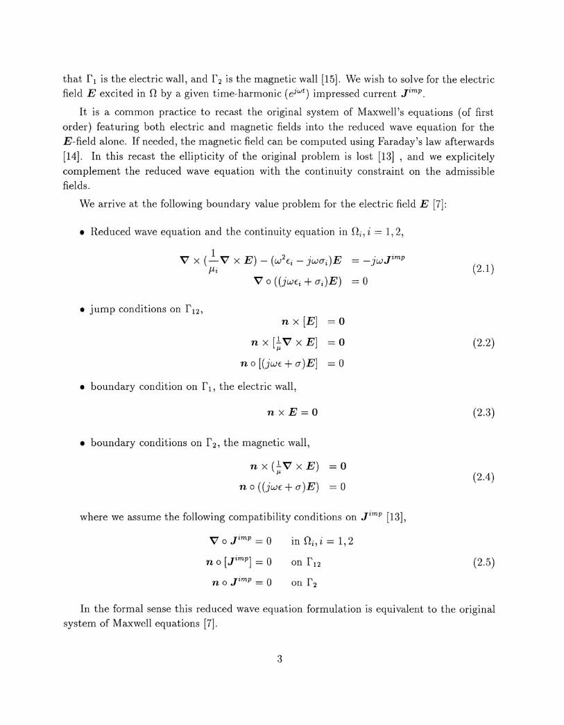
that f 1 is the electric wall, and f 2 is the magnetic wall [15]. We wish to solve for the electricfield E excited in n by a given time-harmonic (ejwt) impressed current fmp.

It is a common practice to recast the original system of Maxwell's equations (of firstorder) featuring both electric and magnetic fields into the reduced wave equation for theE-field alone. If needed, the magnetic field can be computed using Faraday's law afterwards[14]. In this recast the ellipticity of the original problem is lost [13] , and we explicitelycomplement the reduced wave equation with the continuity constraint on the admissiblefields.

We arrive at the following boundary value problem for the electric field E [7]:

• Reduced wave equation and the continuity equation in ni,i = 1,2,

(2.1)VO((jWEi+ai)E) =0

• jump conditions on f12,

n x [E] = 0

n x [IV x E] = 0µ

no [(jwE + a)E] = 0

• boundary condition on f 1, the electric wall,

nxE=O

• boundary conditions on r2, the magnetic wall,

n X (IV x E) = 0µ

no ((jwE+a)E) =0

where we assume the following compatibility conditions on Jimp [13],

(2.2)

(2.3)

(2.4 )

no Jtmp = 0 on f2

(2.5)

In the formal sense this reduced wave equation formulation is equivalent to the originalsystem of Maxwell equations [7].

3

Variational Formulation

We introduce the space of admissible solutions:

(2.6)

equipped with the norm:

(2.7)

and the space of Lagrange multipliers:

(2.8)

with the norm:(2.9)

where1 1

IIgl12,dl = (k t:lgI2dx) 2, IlfI12,µ,n = (k p-llfI2dx) 2 (2.10)

Note that placing the factor w2 in front of IIVpl1 in the definition of the norm in space V isequivalent to replacing the Lagrange multiplier p in the formulation with the product w-2p.The boundary condition in (2.6) is understood in the sense of the generalized Green formula[9], and the boundary condition in (2.8) in the sense of traces.

Wo is a subspace of W:

Wo~{EEW: VxE=O} (2.11 )

We shall assume that the domain n and the boundary conditions are selected in such away 1 that:

Eo E W 0 {:::::::} :J4> E V : Eo = V 4> (2.12)

Following the usual procedure for the mixed methods, we arrive at the following varia-tional formulation:

EEW, pEV

11--(V x E) 0 (V x F) dxnp

-fn(w2t: - jwa)(E + Vp) 0 F dx

= -jw fn(Jimp 0 F) dx, \IF E W

= 0 Vq E V

(2.13)

It has been shown in [7] that at the continuous level Lagrange multiplier p = O.

1We emphasize that n need not be simply connected!

4

Stability, Existence, and Uniqueness

We restrict ourselves to the case of lossless media, only assuming a = O. Both non-zeroconductivity and radiation conditions (for exterior domains) will only improve stability and,in particular, eliminate resonance.In [7] variational problem (2.13) is studied on the Hilbert space W X V with the norm:II(E,p)IIWxV = IIEIIW+llpll~·With assumption (2.12) we can prove the following theorem:

THEOREM 1Let Ai denote the eigenvalues for the eigenvalue problem:

{

E E W, A E C

r ~(V x E) 0 (V x F) dx = A r t:E 0 F dx VF E Wkp kwhere W is the subspace of W, consisting of fields with square integrable curl, 2

(2.14)

(2.15)

Then, for any w2 1= Ai, problem (2.13) possesses a unique solution with a stability estimate:

where

REMARK 1

,=min{ 1 IAi-W21.1 + w2 ' 1 + Ai ' Z = 1,2, ... }

(2.16)

(2.17)

We note that in order to obtain the formulation whose stability properties do not deteri-orate with w --+ 0, it is essential that the continuity condition is enforced explicitely via theLagrange multiplier.

A majority of results reported in the literature, see e.g. [14, 31], are based on thesimplified formulation:

{

EEW

In ~(V x E) 0 (V X F) dx - w2fn t:E 0 F dx = -jw fn (Jimp 0 F) dx,

2For results on existence of the eigenvalues, see (20]

5

VFEW

(2.18)

And for such a formulation:

where. { 2 IAi - w2

1 . }, = mm w , \' Z = 1,2, ...1+ Ai

which means that the stability properties of this formulation deteriorate as w --+ O.

3 Discretization

Galerkin Approximations

(2.19)

(2.20)

I

Introducing finite-dimensional subspaces W heW and Vh C \I, we obtain the approximateproblem by replacing all unknowns and test functions from W, V with their approximationsfrom W h, Vh.

-In (w2t: - jwa)(Eh + Vph) 0 Fh dx

= -jw k(Jimp 0 Fh) dx, VFh E Wh

= 0 Vqh E Vh

(3.1 )

It has been shown in [7] that if a finite element is designed so that the spaces W hand Vh

satisfy the discrete version of (2.12) then the discrete Lagrange multiplier Ph is zero again.(Of course, under the assumption that the impressed current satisfies (2.5) exactly and thatall computations are performed with infinite precision).

An hp-Finite Element Approximation

Further discussion will lead to the case of curvilinear triangular elements. The same approachis valid for rectangles in 2D, and for prisms, cubes and tetrahedra in 3D.

Affine triangular element of variable order

Let k denote a triangle with straight sides ,gi, i = 1,2,3. We associate with the trianglea specific order of approximation P = PK which may vary with element K. Additionally,with each of its sides we associate a possibly different order of approximation Pi, i = 1,2,3,with the assumption that

1 ::::;Pi ::::;P i = 1,2,3

6

(3.2)

Due to approximability requirements, in practice we select p = max{PI, P2, P3}. We introducenow two spaces of element shape functions:

• the scalar space (to approximate the Lagrange multiplier p) identified as the spa.ce ofpolynomials of order p + 1 which, over each of the three sides Si, reduce to polynomialsof order Pi+1,i = 1,2,3,

(3.3)

• the vector space (to approximate the E-field) identified as the space of vector-valuedpolynomials of order p for which the corresponding tangential components, over eachof the three sides Si, reduce to polynomials of order Pi, i = 1,2,3:

(3.4)

Here Ti denotes a tangent vector to side Si, i = 1,2,3.

We also introduce a subspace of W(k):

(3.5)

It is easily shown [7] that

. ' '.' p(p - 1)dlmV(A) = 3 + PI + P2 + P3 + () (3.6)

dimW(k) = (PI + 1) + (P2 + 1) + (P3 + 1) + 3(p - 1) + 2(P + 1)5p + 2) (3.7)

We also have:

THEOREM 2The spaces 1;(k) and W(k) satisfy the same compatibility condition as their continuouscounterparts:

(3.8)

Proof: The proof is trivial. I

In practice both spaces are constructed as spans of predefined element shape functions.For the scalar approximation we use the shape functions introduced in [4].

7

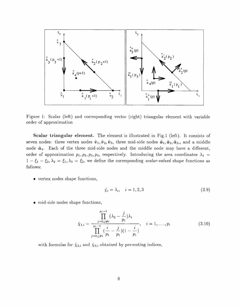
Figure 1: Scalar (left) and corresponding vector (right) triangular element with variableorder of approximation

Scalar triangular element. The element is illustrated in Fig.1 (left). It consists ofseven nodes: three vertex nodes VI, V2, V3, three mid-side nodes 0,1,0,2,0,3" and a middlenode 0,4. Each of the three mid-side nodes and the middle node may have a different,order of approximation PI, P2, P3, P4, respectively. Introducing the area coordinates Al =1 - 6 - 6, A2 = 6, A3 = 6, we define the corresponding scalar-valued shape functions asfollows:

• vertex nodes shape functions,

Xi = Ai, i = 1,2,3

• mid-side nodes shape functions,

(3.9)

Xu =

Pl-1

II (A2 - 1.-)Alj=O,j:f:i PI

Pl-1 i . .'.II (--1.-)(1- 2-)]=O,j:f:i PI PI PI

i= 1, ... ,PI (3.10)

with formulas for ~b,iand X3,i obtained by permuting indices,

8

• middle node shape functions,

i-I m j-l n k-l mII(AI - -) II(A2 - -) II(A3 --)

m=O P n=O P 1=0 PX4,i,j,k = i-I i m j-l j n k-l k l

II (- - -) II(- - -) II(- --)m=O P P n=O P P 1=0 P P

with 1 :::;i, j, k :::; P, i + j + k = P + 1.

(3.11)

Vector triangular element: The vector element is illustrated in Fig.1 (right) . Formally,it consists of seven nodes: three tangential mid-side nodes o,~,o,~,o,~, three normal mid-sidenodes o,~,o,~,o,~, and again the middle node 0,4. The tangential nodes are of order PI, P2, P3,resp., whereas all normal nodes and the middle node are of order p. Next, similarly to thescalar approximation, for each of the nodes we introduce the corresponding Lagrangian nodeso'~,j' o'~j' o'4,j. Note that the Lagrangian nodes for the tangential mid-side nodes include thevertices. Vector shape functions have two components. Each component is constructed fromthe polynomials of the same type shown above for the case of scalar shape functions.

The degrees of freedom for the scalar and vector element will be discussed in conjunctionwith the general case of curvilinear elements.

Curvilinear Triangular Element

Let a curvilinear triangle I< be the image of some one-to-one C2-smooth map T definedon J{:

T: It" ---7 J{ (3.12)

Following [2, 8], we introduce the space of vector shape functions over the curvilinear elementIt" as:

Here dT(x) is the Jacobian matrix of the map T at the point x E k and [tdT(x)]-l is theinverse of its transpose. In other words, vector functions defined on J{ are transformed fromk like gradients [32].

The space of scalar shape functions is defined as usually by the composition with T:

V(I<) ~ {q : I< --+ R, :Jq E v(f{), q(T(x)) = q(x), Vx E k} (3.14)

Since T is one-to-one, dimV(I<) = dimV(k), and dimW(K) = dimW(f{).It has been shown in [8] that V x F = det(dTr1(V x F). Therefore, we can introduce

the subspace of curl-free vectors in W(K) as:

9

We will need the following

THEOREM 3

¢ E V(J() {:::::::}V¢ E Wo(J() (3.16)

Proof: Definitions (3.13)-(3.15), Theorem 2, and the chain rule of differentiation leadstraight to the result above. I

Scalar Degrees of Freedom

The scalar shape functions on J( are introduced according to the definition of V( J()(3.14). They may no longer be polynomials. The choice of the actual degrees of freedom(dof) is not unique but it should reflect global continuity requirements.

THEOREM 4The following Lagrangian do! are V( J()-unisolvent

q --+ q( Vi)

q --+ q( ai,j)

q --+ q( a4,j)

i = 1,2,3

ai,j = T( o'i,j) i = 1,2,3, j = 1, ... ,Pi

a4,j = T(o'4,j) j = 1, ... ,p(p - 1)/2

(3.17)

where Vi, o'i,j, o'4,j have been introduced in the definition of the scalar shape functions on i,.".

Proof: As the number of dof equals exactly the dimension of space V( J(), compare with(3.6), it remains to check that they are linearly independent. This means that if they are allzero for a function q E V(J(), the function q must be zero. The assertion follows immediatelyfrom (3.3) and (3.14) I

With our choice of dof on V(J(), in order to enforce the global continuity of the scalarapproximation we assume that the function values at the vertex nodes and at the mid-sidenodes are shared by adjacent elements.

Vector Degrees of Freedom

First, we consider seven "logical" nodes, which are: three tangential mid-side nodesat, a~, a~, three normal mid-side nodes a~, a~, a~, and again the middle node a4. Next, sim-

10

ilarly to the scalar approximation, for each of the formal nodes we define the correspondingL . d t T(At) n T(An) T(A) 'th{At An A } lA,agranglan no es as: ai,j = ai,j' ai,j = ai,j' a4,j = a4,j, WI ai,j' ai,j' a4,j C 1

We note that the Lagrangian nodes for the tangential mid-side nodes include the vertices.The corresponding dof are defined as follows:

• tangential dof:

• normal dof:

• middle dof

F --+ F(at .) 0 TiJ· i = 1, 2,3,j = 0, ... ,PiZ,) ,

F --+ F(a7,j) 0 ni,j i= 1,2,3,j = 1, ... ,p-l

F --+ F(a4,j) 0 ik k = 1,2,j = 1, ... , (p - 2)(p - 1)/2

(3.18)

(3.19)

(3.20)

Here Ti,j denotes tangential unit vectors constructed at points a~,j and directed from thevertex node with a smaller (global) number to the vertex node with a greater number, ni,j

denotes outward normal unit vectors constructed at points a~j' and ik, k = 1,2 stands forthe global cartesian unit vectors. Note that for elements with straight edges vectors Ti,j andni,j are independent of index j.

THEOREM 5The dof described by (3.18)-(3.20) are W(I<)-unisolvent.

Proof: As for the scalar case, the number of dof equals dimW(I<). We must check thatthe dof are linearly independent. Again, let us assume that for some F E W(I<) all dof arezero. We need to show that F is a zero-vector. The relation between unit tangent vectorson I< and f< is given by [9]:

T(T(x)) = dT(x)f(x)

And for the unit normal vectors [9]:

where 11.11 denotes 2D Eucledian norm.

From (3.13),(3.4), it is clear that for the vector F corresponding to F:

F(a~)fi = 0, i = 1,2,3,j = 0, ... ,Pi

11

(3.21)

(3.22)

(3.23)

From (3.23) and (3.7) it follows that the tangential component of F vanishes along all threesides of k. This fact together with (3.23) and (3.22) leads to:

F( a~Jni = 0, i = 1,2,3, j = 0, ... ,p - 1 (3.24)

We conclude from (3.24),(3.4), and (3.7) that the normal component of F also vanishes alongall three sides.

Let us consider now the middle node. From (3.13),(3.4),(3.7), and since [tdT]-l has fullrank we conclude that F must vanish at the middle node as well. Therefore, F is zero onk, this in turn means that F on J{ is also zero. I

In order to construct an internal polynomial approximation of H( curl)-space, the con-tinuity of the "tangential" components of vector-functions must be enforced. Therefore weassume that the values of the tangential dof are shared by adjacent elements. To demon-strate that the approximation remains H (curl )-conforming for parametric maps we consider2 adjacent curvilinear elements J{l and 1\.'2 with the common side !(12 = Rl nR2. The mapsTi: ki ---+ J{i,i = 1,2 are identical along J{12, therefore ((dTl - dT2)T)IK12 = O.Let F be a vector field on J{l U J{2' Given that:

(3.25)

we use (3.21) to show that (Ji\(aU - Ji\(aU)Ti = 0 j = O'''',Pi for Fi correspondingto FIKi' i = 1,2. Since Ti is a non-zero vector and F 1 - F 2 is a polynomial of degreePi, it follows that Fl = F2 restricted to k12. Applying again (3.21) we conclude thatFIK1(X)T(X) = FIK2(x)T(x) Vx E J{12, therefore the approximation is indeed H(curl)-conforming.

REMARK 2 Let us note that the Lagrangian dof for scalar and vector-valued functionsdo not coincide with the dual basis to the original shape functions. Consequently, therestrictions to an element of the global basis functions (which are dual to the global dof)do not coincide with the original element shape functions and the generalized assemblyingprocedure discussed in [7] must be applied. I

Convergence Analysis

Let n be a bounded domain with piece-wise smooth, possibly curvilinear boundary. Let Thbe a triangulation of the domain. We define the FE spaces W heW and VhC Vas:

(3.26)

12

and(3.27)

We also introduce the subspace of curl-free functions in W h:

(3.28)

We have the following essential compatibility result:

THEOREM 6

(3.29)

Proof: Let us take any 4> E Vh. By (3.26) and (3.16) V4> E Wo, by (3.26) and (3.8)V4>IK E Wo(I<), VI< E~. Therefore, by (3.28) V4> E WOh.

Conversely, let us take any E E WOh. By (3.28) and (3.16) :J4> E V: V4> = E. By(3.28), (3.8) and since the tangential component of E is continuous across element interfaces:Vf{ E ~ :J1/Jk E V(f{), such that V1/Jk = ElK and 1/Jk = 4>IK. Therefore by (3.26) 4> E Vh.I

We derive the following estimate for the discrete LBB constant using the same techniqueas for its continuous counterpart, [7]:

1 IAih-

w21 i=1,2, ... }

ih ~ min{ 1 + w2' 1+ Aih ' (3.30)

where Aih denotes the discrete eigenvalues resulting for the Galerkin approximation of (2.14).We emphasize the essential role of condition (3.29) in deriving the result above.

Combining the discrete stability result with the classical theory on asymptotic conver-gence (see e.g. [5]), we arrive at the final convergence result.

THEOREM 7There exists a threshold value ho and a constant C, independent of h, such that

for every h ~ ho. Constant C depends upon frequency w but is bounded away from infinityfor w --+ O.

13

Theoretically, since P = 0 and with condition (3.29) satisfied, Ph = 0 as well, and (3.31)reduces to the estimate:

(3.32)

In practice, of course, due to the round-off and integration error and due to possible con-tamination of input data (impressed current) Ph is never exactly zero.

REMARK 3 hp-error estimates. Theorem 7, when combined with the interpolationerror estimates for hp-approximations, see [1, 24], results in standard hp-error estimates,with exponential rates of convergence for analytic solutions. I

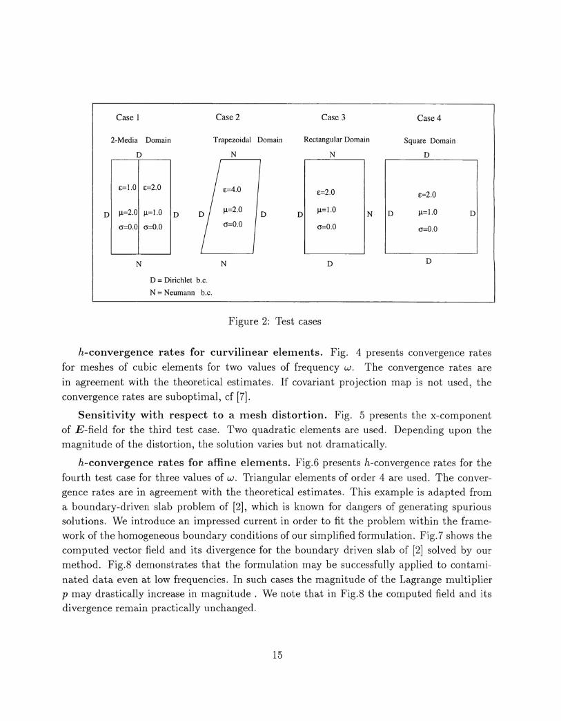
4 Numerical Experiments

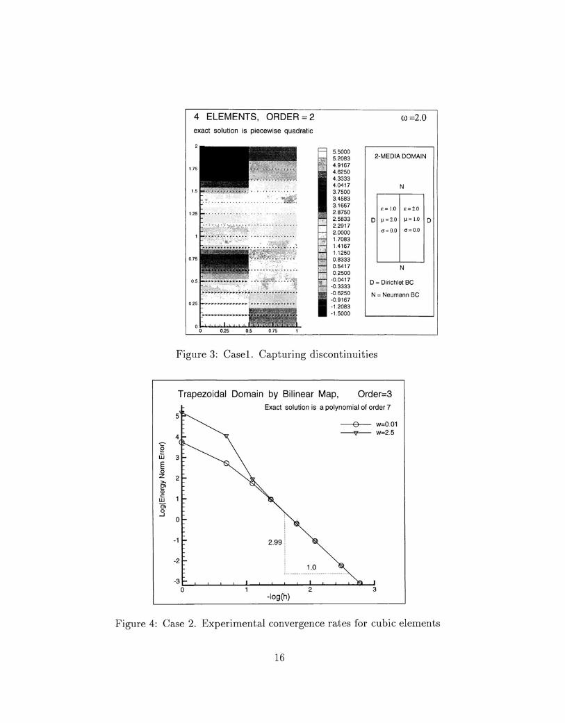
Test cases. All presented results are two-dimensional. Fig. 2 displays four test cases. Thecorresponding exact solutions for the first three cases are polynomials of order 2, 7, and 5,respectively. In the first case, due to the discontinuity of constants p and t:, the horizontalcomponent of the solution has a jump across the vertical interface. For the square domainthe exact solution is composed of trigonometric and hyperbolic sines and cosines (dependingon w).

In [7] the reader will find a short discussion on the geometry representation and initialmesh generation used in the experiments.

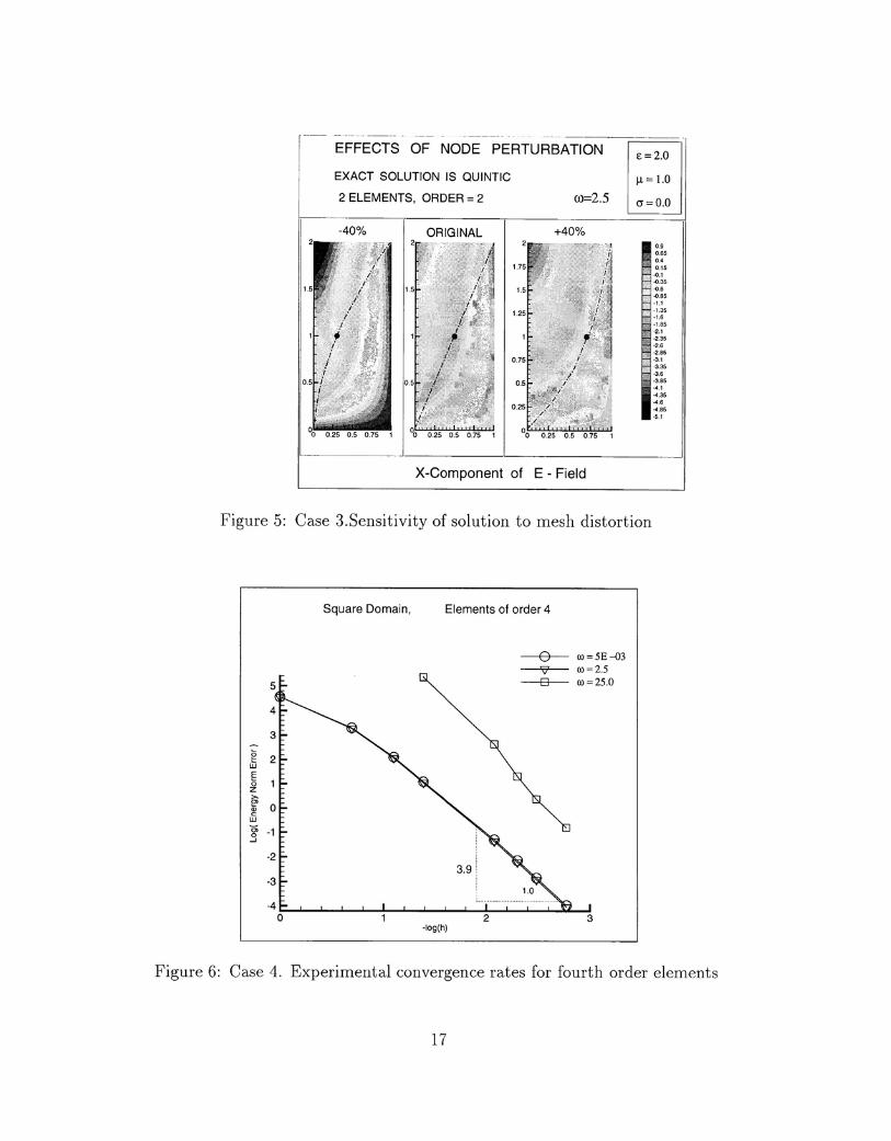
The parametrization maps are linear for cases 1 and 4. The resulting mesh consists ofaffine elements. Bilinear maps are used to model the domains for cases 2 and 3, and theresulting triangular elements have curved sides.

Discontinuous solutions. We begin with a simple illustration of the fact that theformulation can handle discontinuous solutions. Fig. 3 displays the x-component of theE-field reproduced using a mesh of quadratic elements.

14

£=4.0

In£=2.0

µ=2.0D

µ=1.0

0=0.0 0=0.0

Case 1

2-Media Domain

D

£=1.0 £=2.0

DIµ=2.0 µ=1.0

ID0=0.0 0=0.0

N

D = Dirichlet b.c.

N = Neumann b.c.

Case 2

Trapezoidal Domain

N

N

Case 3

Rectangular Domain

N

N ID

D

Case 4

Square Domain

D

£=2.0

µ=1.0

0=0.0

D

D

Figure 2: Test cases

h-convergence rates for curvilinear elements. Fig. 4 presents convergence ratesfor meshes of cubic elements for two values of frequency w. The convergence rates arein agreement with the theoretical estimates. If covariant projection map is not used, theconvergence rates are suboptimal, cf [7].

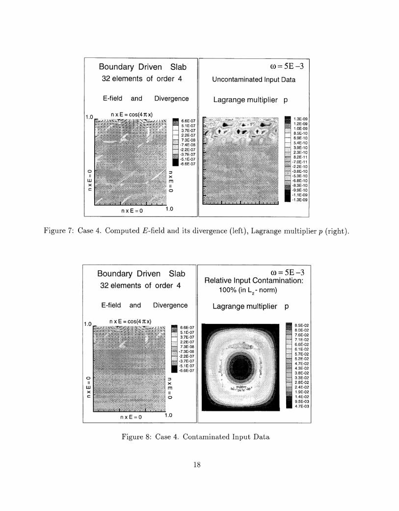
Sensitivity with respect to a mesh distortion. Fig. 5 presents the x-componentof E-field for the third test case. Two quadratic elements are used. Depending upon themagnitude of the distortion, the solution varies but not dramatically.

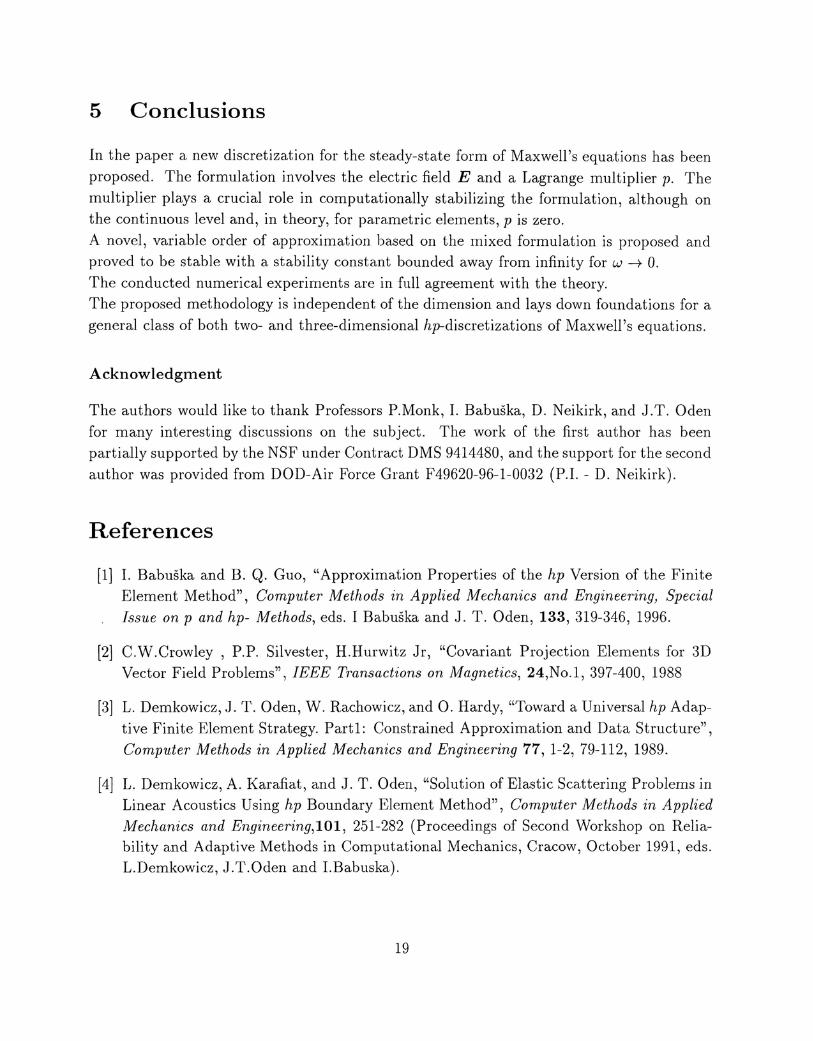
h-convergence rates for affine elements. Fig.6 presents h-convergence rates for thefourth test case for three values of w. Triangular elements of order 4 are used. The conver-gence rates are in agreement with the theoretical estimates. This example is adapted froma boundary-driven slab problem of [2], which is known for dangers of generating spurioussolutions. We introduce an impressed current in order to fit the problem within the frame-work of the homogeneous boundary conditions of our simplified formulation. Fig.7 shows thecomputed vector field and its divergence for the boundary driven slab of [2] solved by ourmethod. Fig.8 demonstrates that the formulation may be successfully applied to contami-nated data even at low frequencies. In such cases the magnitude of the Lagrange multiplierp may drastically increase in magnitude. We note that in Fig.8 the computed field and itsdivergence remain practically unchanged.

15

4 ELEMENTS, ORDER = 2exact solution is piecewise quadratic

5.50005.20834.91674.62504.33334.04173.75003.45833.16672.87502.58332.29172.00001.70831.41671.12500.83330.54170.2500

-0.0417-0.3333-0.6250-0.9167-1.2083-1.5000

(0 =2.0

2-MEDIA DOMAIN

N

E = 1.0 I E = 2.0

D I µ= 2.0 µ= 1.0 I D,,=0.0 "=0.0

N

D = Dirichlet BC

N = Neumann BC

Figure 3: Casel. Capturing discontinuities

Trapezoidal Domain by Bilinear Map, Order=3Exact solution is a polynomial of order 7

ew 3E0z 2>-OlQ;c:

WOi0-l

0

-1

-2

-30

2.99

e-- w=O.01- w=2.5

-Iog(h)

Figure 4: Case 2. Experimental convergence rates for cubic elements

16

EFFECTS OF NODE PERTURBATION E=2.0

EXACT SOLUTION IS QUINTIC

2 ELEMENTS, ORDER = 2 OJ=2.5µ= 1.0

(J = 0.0

-40% ORIGINAL +40%

0.25 0.5 0.75 1 I 00 0.25 0.5 0.75 1 0.25 0.5 0.75 1

0.90.650.'0.15

'(1.1.(J.35.(J.8

-0.85-1.1-1.35-1.6

-1.85-2.1-2.35-2.6·2.85-3.1-3.35-3.6-3.85-4.1

-4.35-4.8-4B5-5.1

X-Component of E - Field

Figure 5: Case 3.Sensitivity of solution to mesh distortion

Square Domain, Elements of order 4

(0 = 5E--{)3(0=2.5(0=25.0

e'V'p

3

4

5

e 2WE(; 1z>-Q)

Ii; 0cW

g; -1-'

-2

-3

-40 1 2 3

-Iog(h)

Figure 6: Case 4. Experimental convergence rates for fourth order elements

17

Boundary Driven Slab32 elements of order 4

ro=5E-3Uncontaminated Input Data

E-field and Divergence Lagrange multiplier p

1.0

oII

UJXC

n x E = cos(41tx)6.6E-075.1E-073.7E-072.2E-077.3E-08·7.4E-08-22E-07-3.7E-07-5.1E-07-6.6E-07

1.3E-091.2E-0910E-098.5E-106.9E-105.4E-103.9E-102.3E-108.2E-11-7.0E-11-2.2E-10-3.8E-10-5.3E-10-6.8E-10-8.3E-1O-9.9E-10·1.1E-09-1.3E·09

nxE=O 1.0

Figure 7: Case 4. Computed E-field and its divergence (left), Lagrange multiplier p (right).

Boundary Driven Slab32 elements of order 4

ro=5E-3Relative Input Contamination:

100% (in L2

- norm)

E-field and Divergence Lagrange multiplier p

1.0

oII

UJXC

n x E = cos(41tx)6.6E-075.1E-073.7E-072.2E-077.3E·08-7.3E-08·2.2E-07-3.7E-07-5.1E-07-6.6E-07

8.5E-028.0E-027.6E-027.1E-026.6E-026.1E-025.7E-025.2E-024.7E-024.3E-023.8E-023.3E-022.8E·022.4E-021.9E-021.4E-029.5E-034.7E-03

nxE=O 1.0

Figure 8: Case 4. Contaminated Input Data

18

5 Conclusions

In the paper a new discretization for the steady-state form of Maxwell's equations has beenproposed. The formulation involves the electric field E and a Lagrange multiplier p. Themultiplier plays a crucial role in computationally stabilizing the formulation, although onthe continuous level and, in theory, for parametric elements, p is zero.A novel, variable order of approximation based on the mixed formulation is proposed andproved to be stable with a stability constant bounded away from infinity for w --+ O.The conducted numerical experiments are in full agreement with the theory.The proposed methodology is independent of the dimension and lays down foundations for ageneral class of both two- and three-dimensional hp-discretizations of Maxwell's equations.

Acknowledgment

The authors would like to thank Professors P.Monk, I. Babuska, D. Neikirk, and J.T. Odenfor many interesting discussions on the subject. The work of the first author has beenpartially supported by the NSF under Contract DMS 9414480, and the support for the secondauthor was provided from DOD-Air Force Grant F49620-96-1-0032 (P.I. - D. Neikirk).

References

[1] 1. Babuska and B. Q. Guo, "Approximation Properties of the hp Version of the FiniteElement Method", Computer Methods in Applied Mechanics and Engineering, SpecialIssue on p and hp- Methods, eds. I Babuska and J. T. Oden, 133, 319-346, 1996.

[2] C.W.Crowley , P.P. Silvester, H.Hurwitz Jr, "Covariant Projection Elements for 3DVector Field Problems", IEEE Transactions on Magnetics, 24,No.1, 397-400, 1988

[3] L. Demkowicz, J. T. Oden, W. Rachowicz, and O. Hardy, "Toward a Universal hp Adap-tive Finite Element Strategy. Partl: Constrained Approximation and Data Structure",Computer Methods in Applied Mechanics and Engineering 77, 1-2, 79-112, 1989.

[4] L. Demkowicz, A. Karafiat, and J. T. Oden, "Solution of Elastic Scattering Problems inLinear Acoustics Using hp Boundary Element Method", Computer Methods in AppliedMechanics and Engineering,101, 251-282 (Proceedings of Second Workshop on Relia-bility and Adaptive Methods in Computational Mechanics, Cracow, October 1991, eds.L.Demkowicz, J.T.Oden and 1.Babuska).

19

[5] L. Demkowicz, "Asymptotic Convergence in Finite and Boundary Element Methods:Part 1: Theoretical Results", Computers and Mathematics with Applications, 27, 12,69-84, 1994.

[6] L. Demkowicz, "A Modified FE Assembling Procedure with Applications to Electromag-netics, Acoustics and hp-Adaptivity", Mathematics of Finite Elements with Application,ed. J. R. Whiteman, John Wiley and Sons Ltd., in print.

[7] L. Demkowicz, L. Vardapetyan , "Modeling of Electromagnetic Absoption/ScatteringProblems Using hp-adaptive Finite Elements", Computer Methods in Applied Mechanicsand Engineering, to appear in 1997.

[8] F.Dubois, "Discrete Vector Potential Representation of a Divergence-Free Vector Fieldin Three-Dimensional Domains: Numerical Analysis of a Model Problem", SIAMJ.Numerical Analysis,v.27,No.5, 1103-1141, 1990

[9] V. Girault, and P.A. Raviart, Finite Element Methods for Navier-Stokes Euations,Springer- Verlag, Berlin, 1986.

[10] C. Hazard, and S. Lohrengel, "How to Use Standard Lagrange Finite Elements forSolving Maxwell's Equations", MAFELAP 1996.

[11] D.J. Hoppe, L.W. Epp, and J.F. Lee, "A Hybrid Symmetric FEM/MOM FormulationApplied to Scattering by Inhomogeneous Bodies of Revolution", IEEE Transactions onAntennas and Propagation, 42, 6, 798-805, 1994.

[12] F. Ihlenburg and 1. Babuska, "Finite Element Solution to the Helmholtz Equation withHigh Wave Number. Part I: The h-Version of the FEM", Institute for Physical Scienceand Technology, Technical Note BN-1159, November 1993.

[13] B.N. Jiang, J. Wu, and L.A. Povinelli, "The Origin of Spurious Solutions in Computa-tional Electromagnetics", Journal of Computational Physics 125, 104-123, 1996.

[14] J. Jin, The Finite Element Method in Electromagnetics, John Wiley & Sons, Inc., NewYork 1993.

[15] J .F. Lee, "Analysis of Passive Microwave Devices by Using Three-Dimensional Tangen-tial Vector Finite Elements", International Journal of Numerical Modeling: Electronicnetworks, Devices and Fields, 3, 235-246, 1990.

[16] J .F. Lee, D.K. Sun, and Z.J. Cendes, "Tangential Vector Finite Elements for Elec-tromagnetic Field Computation", IEEE Transactions on Magnetics, 27, 5, 4032-4035,1991.

20

[17] J .F. Lee, D.K. Sun, and Z.J. Cendes, "Full-Wave Analysis of Dielectric WaveguidesUsing Tangential Vector Finite Elements", IEEE Transactions on Microwave Theoryand Techniques, 39, 8, 1991.

[18] J .F. Lee, R. Palandech, and R. Mittra, "Modeling Three-Dimensional Discontinuities inWaveguides Using Nonorthogonal FDTD Algorithm", IEEE Transcations on MicrowaveTheory and techniques, 40, 2, 346-352, 1992.

[19] J .F. Lee, C.M. Wilkins, and R. Mittra, "Finite-Element Analysis of Axisymmetric Cav-ity resonator Using a Hybrid Edge Element Technique", IEEE Transactions on Mi-crowave Theory and Techniques, 41, 11, 1993.

[20] R. Leis, Initial Boundary Value Problems in Mathematical Physics, John Wiley andSons, New York 1986

[21] P. Monk, "A Finite Element Method for Approximating the Time-Harmonic MaxwellEquations", Numerische mathematik, 63, 243-261, 1992.

[22] P. Monk, "Analysis of a Finite Element method for Maxwell's Equations", SIAM Jour-nal of Numerical Analysis, 29, 3, 714-729, 1992.

[23] P. Monk, "An Analysis of Nedelec's Method for the Spatial Discretization of Maxwell'sEquations", Journal of Computational and Applied Mathematics, 47, 101-121, 1993.

[24] P. Monk, "On the p- and hp-extension of Nedelec's Curl-Conforming Elements", Jour-nal of Computational and Applied Mathematics, 53, 117-137, 1994.

[25] P. Monk, "Superconvergence of Finite Element Approximations to Maxwell's Equa-tions", Numerical Methods for Partial Differential Equations, 10, 793-812, 1994.

[26] G. Mur, "Finite Element Methods for Electromagnetic Field Computations", MAFE-LAP 1996.

[27] J.C. Nedelec, "Computation of Eddy Currents on a Surface in IB? by Finite ElementMethods", SIAM Journal of Numerical Analysis, 15,3, 580-594, 1978.

[28] J .C. Nedelec, "Mixed Finite Elements in JR3", Numerische Mathematik, 35, 315-341,1980.

[29] J .C. Nedelec, "A New Family of Mixed Finite Elements in JR3", NumeTische Mathematik,50, 57-81, 1986.

21

[30] J. T. Oden, L. Demkowicz, W. Rachowicz and T. A. Westermann, "Towards a Universalh-p Adaptive Finite Element Strategy, Part 2. A Posteriori Error Estimation," Camp.Meth. Appl. Meth. Eng., 77, 113-180, 1989.

[31] P.P. Silvester, and G. Pelosi (eds.), Finite Elements for Wave Electromagnetics, IEEEPress, New York, 1994.

[32] V.l. Smirnov, A Course of Higher Mathematics, v.3, Pergamon Press, Oxford, 1964

22