introduction to the finite element method in electromagnetics
TRANSCRIPT

P1: IML/FFX P2: IML/FFX QC: IML/FFX T1: IML
MOBK021-FM MOBK021-Polycarpou.cls April 29, 2006 20:15
Introduction to the Finite ElementMethod in Electromagnetics
i

P1: IML/FFX P2: IML/FFX QC: IML/FFX T1: IML
MOBK021-FM MOBK021-Polycarpou.cls April 29, 2006 20:15
Copyright © 2006 by Morgan & Claypool
All rights reserved. No part of this publication may be reproduced, stored in a retrieval system, or transmitted in
any form or by any means—electronic, mechanical, photocopy, recording, or any other except for brief quotations in
printed reviews, without the prior permission of the publisher.
Introduction to the Finite Element Method in Electromagnetics
Anastasis C. Polycarpou
www.morganclaypool.com
1598290460 paper Polycarpou
1598290479 ebook Polycarpou
DOI 10.2200/S00019ED1V01Y200604CEM004
A Publication in the Morgan & Claypool Publishers’ series
SYNTHESIS LECTURES ON COMPUTATIONAL ELECTROMAGNETICS
Lecture #4
First Edition
10 9 8 7 6 5 4 3 2 1
Printed in the United States of America
ii
P1: IML/FFX P2: IML/FFX QC: IML/FFX T1: IML
MOBK021-FM MOBK021-Polycarpou.cls April 29, 2006 20:15
Introduction to the Finite ElementMethod in Electromagnetics
Anastasis C. Polycarpou
Intercollege, Cyprus
SYNTHESIS LECTURES ON COMPUTATIONAL ELECTROMAGNETICS #4
M&C
Morgan &Claypool Publishers
iii

P1: IML/FFX P2: IML/FFX QC: IML/FFX T1: IML
MOBK021-FM MOBK021-Polycarpou.cls April 29, 2006 20:15
To my parents, and to my wife and daughter
iv
P1: IML/FFX P2: IML/FFX QC: IML/FFX T1: IML
MOBK021-FM MOBK021-Polycarpou.cls April 29, 2006 20:15
v
ABSTRACTThis series lecture is an introduction to the finite element method with applications in electro-
magnetics. The finite element method is a numerical method that is used to solve boundary-value
problems characterized by a partial differential equation and a set of boundary conditions. The
geometrical domain of a boundary-value problem is discretized using sub-domain elements,
called the finite elements, and the differential equation is applied to a single element after it is
brought to a “weak” integro-differential form. A set of shape functions is used to represent the
primary unknown variable in the element domain. A set of linear equations is obtained for each
element in the discretized domain. A global matrix system is formed after the assembly of all
elements.
This lecture is divided into two chapters. Chapter 1 describes one-dimensional boundary-
value problems with applications to electrostatic problems described by the Poisson’s equation.
The accuracy of the finite element method is evaluated for linear and higher order elements
by computing the numerical error based on two different definitions. Chapter 2 describes
two-dimensional boundary-value problems in the areas of electrostatics and electrodynamics
(time-harmonic problems). For the second category, an absorbing boundary condition was
imposed at the exterior boundary to simulate undisturbed wave propagation toward infinity.
Computations of the numerical error were performed in order to evaluate the accuracy and
effectiveness of the method in solving electromagnetic problems. Both chapters are accompa-
nied by a number of Matlab codes which can be used by the reader to solve one- and two-
dimensional boundary-value problems. These codes can be downloaded from the publisher’s
URL: www.morganclaypool.com/page/polycarpou
This lecture is written primarily for the nonexpert engineer or the undergraduate or grad-
uate student who wants to learn, for the first time, the finite element method with applications
to electromagnetics. It is also targeted for research engineers who have knowledge of other
numerical techniques and want to familiarize themselves with the finite element method. The
lecture begins with the basics of the method, including formulating a boundary-value problem
using a weighted-residual method and the Galerkin approach, and continues with imposing all
three types of boundary conditions including absorbing boundary conditions. Another impor-
tant topic of emphasis is the development of shape functions including those of higher order. In
simple words, this series lecture provides the reader with all information necessary for someone
to apply successfully the finite element method to one- and two-dimensional boundary-value
problems in electromagnetics. It is suitable for newcomers in the field of finite elements in
electromagnetics.

P1: IML/FFX P2: IML/FFX QC: IML/FFX T1: IML
MOBK021-FM MOBK021-Polycarpou.cls April 29, 2006 20:15
KEYWORDSBoundary-value problems (BVPs), Finite element method (FEM),
Galerkin approach, Higher order elements, Linear elements,
Numerical methods, Shape/interpolation functions, Weak formulation
vi

P1: IML/FFX P2: IML/FFX QC: IML/FFX T1: IML
MOBK021-FM MOBK021-Polycarpou.cls April 29, 2006 20:15
vii
Contents
1. One-Dimensional Boundary-Value Problems . . . . . . . . . . . . . . . . . . . . . . . . . . . . . . . . . . . 1
1.1 Introduction . . . . . . . . . . . . . . . . . . . . . . . . . . . . . . . . . . . . . . . . . . . . . . . . . . . . . . . . . . . . . 1
1.2 Electrostatic BVP and the Analytical Solution. . . . . . . . . . . . . . . . . . . . . . . . . . . . . . .1
1.3 The Finite Element Method . . . . . . . . . . . . . . . . . . . . . . . . . . . . . . . . . . . . . . . . . . . . . . 3
1.4 Domain Discretization . . . . . . . . . . . . . . . . . . . . . . . . . . . . . . . . . . . . . . . . . . . . . . . . . . . . 5
1.5 Interpolation Functions . . . . . . . . . . . . . . . . . . . . . . . . . . . . . . . . . . . . . . . . . . . . . . . . . . . 5
1.6 The Method of Weighted Residual: The Galerkin Approach . . . . . . . . . . . . . . . . . 7
1.7 Assembly of Elements . . . . . . . . . . . . . . . . . . . . . . . . . . . . . . . . . . . . . . . . . . . . . . . . . . . 13
1.8 Imposition of Boundary Conditions . . . . . . . . . . . . . . . . . . . . . . . . . . . . . . . . . . . . . . . 19
1.8.1 Dirichlet Boundary Conditions . . . . . . . . . . . . . . . . . . . . . . . . . . . . . . . . . . . 19
1.8.2 Mixed Boundary Conditions . . . . . . . . . . . . . . . . . . . . . . . . . . . . . . . . . . . . . . 22
1.9 Finite Element Solution of the Electrostatic Boundary-Value Problem . . . . . . . 22
1.10 One-Dimensional Higher Order Interpolation Functions . . . . . . . . . . . . . . . . . . . 29
1.10.1 Quadratic Elements . . . . . . . . . . . . . . . . . . . . . . . . . . . . . . . . . . . . . . . . . . . . . . 30
1.10.2 Cubic Elements . . . . . . . . . . . . . . . . . . . . . . . . . . . . . . . . . . . . . . . . . . . . . . . . . 33
1.11 Element Matrix and Right-Hand-Side Vector Using Quadratic Elements . . . . 36
1.12 Element Matrix and Right-Hand-Side Vector Using Cubic Elements . . . . . . . . 39
1.13 Postprocessing of the Solution: Quadratic Elements . . . . . . . . . . . . . . . . . . . . . . . . 39
1.14 Postprocessing of the Solution: Cubic Elements . . . . . . . . . . . . . . . . . . . . . . . . . . . . 47
1.15 Software . . . . . . . . . . . . . . . . . . . . . . . . . . . . . . . . . . . . . . . . . . . . . . . . . . . . . . . . . . . . . . . 48
2. Two-Dimensional Boundary-Value Problems . . . . . . . . . . . . . . . . . . . . . . . . . . . . . . . . . . 51
2.1 Introduction . . . . . . . . . . . . . . . . . . . . . . . . . . . . . . . . . . . . . . . . . . . . . . . . . . . . . . . . . . . . 51
2.2 Domain Discretization. . . . . . . . . . . . . . . . . . . . . . . . . . . . . . . . . . . . . . . . . . . . . . . . . . .52
2.3 Interpolation Functions . . . . . . . . . . . . . . . . . . . . . . . . . . . . . . . . . . . . . . . . . . . . . . . . . . 54
2.3.1 Linear Triangular Element . . . . . . . . . . . . . . . . . . . . . . . . . . . . . . . . . . . . . . . .54
2.3.2 Bilinear Quadrilateral Element . . . . . . . . . . . . . . . . . . . . . . . . . . . . . . . . . . . . 59
2.4 The Method of Weighted Residual: The Galerkin Approach . . . . . . . . . . . . . . . . 61
2.5 Evaluation of Element Matrices and Vectors . . . . . . . . . . . . . . . . . . . . . . . . . . . . . . . 66
2.5.1 Linear Triangular Elements . . . . . . . . . . . . . . . . . . . . . . . . . . . . . . . . . . . . . . . 67
2.5.2 Bilinear Quadrilateral Elements . . . . . . . . . . . . . . . . . . . . . . . . . . . . . . . . . . . 75
2.6 Assembly of the Global Matrix System . . . . . . . . . . . . . . . . . . . . . . . . . . . . . . . . . . . . 86

P1: IML/FFX P2: IML/FFX QC: IML/FFX T1: IML
MOBK021-FM MOBK021-Polycarpou.cls April 29, 2006 20:15
viii CONTENTS
2.7 Imposition of Boundary Conditions . . . . . . . . . . . . . . . . . . . . . . . . . . . . . . . . . . . . . . . 90
2.8 Solution of the Global Matrix System . . . . . . . . . . . . . . . . . . . . . . . . . . . . . . . . . . . . . 90
2.9 Postprocessing of the Results . . . . . . . . . . . . . . . . . . . . . . . . . . . . . . . . . . . . . . . . . . . . . 91
2.10 Application Problems . . . . . . . . . . . . . . . . . . . . . . . . . . . . . . . . . . . . . . . . . . . . . . . . . . . . 92
2.10.1 Electrostatic Boundary-Value Problem . . . . . . . . . . . . . . . . . . . . . . . . . . . . . 92
2.10.2 Two-Dimensional Scattering Problem . . . . . . . . . . . . . . . . . . . . . . . . . . . . . 97
2.11 Higher Order Elements . . . . . . . . . . . . . . . . . . . . . . . . . . . . . . . . . . . . . . . . . . . . . . . . 105
2.11.1 A Nine-Node Quadratic Quadrilateral Element . . . . . . . . . . . . . . . . . . . 106
2.11.2 A Six-Node Quadratic Triangular Element . . . . . . . . . . . . . . . . . . . . . . . .108
2.11.3 A Ten-Node Cubic Triangular Element . . . . . . . . . . . . . . . . . . . . . . . . . . .110
2.12 Software . . . . . . . . . . . . . . . . . . . . . . . . . . . . . . . . . . . . . . . . . . . . . . . . . . . . . . . . . . . . . . 111
P1: IML/FFX P2: IML/FFX QC: IML/FFX T1: IML
MOBK021-FM MOBK021-Polycarpou.cls April 29, 2006 20:15
ix
Preface
This book was written as an introductory text to the finite element method in electromagnetics.
The finite element method has been widely used in computational electromagnetics for the last
40–50 years with an impressive number of quality publications on the subject in the late 1980s
and 1990s. It is a highly versatile numerical method that has received considerable attention
by scientists and researchers around the world after the latest technological advancements
and computer revolution of the twentieth century. The main concept of the finite element
method is based on subdividing the geometrical domain of a boundary-value problem into
smaller subdomains, called the finite elements, and expressing the governing differential equation
along with the associated boundary conditions as a set of linear equations that can be solved
computationally using linear algebra techniques. The subject of the finite element method in
electromagnetics is very broad and covers a wide range of topics that are impossible to cover in
a short introductory book. Some of these topics include vector elements, eigenvalue problems,
axisymmetric problems, three-dimensional scattering and radiation problems, microwave and
millimeter wave circuits, absorbing boundary conditions and the perfectly matched layer, hybrid
methods, and a few more. The purpose of this book is primarily the introduction of this
numerical method to the undergraduate student and the nonexpert working engineer who may
be using commercial finite element codes or simply is interested in learning this method for
the first time. Therefore, emphasis was placed on writing a book that is limited in size but
not in substance, characterized by simplicity and clarity, free of advanced mathematics and
complex variational formulations, self-contained, and effective in teaching the reader the basics
of the method. It can be considered as a first book in learning the finite element method with
applications in electromagnetics. More advanced books may follow to cover specific topics that
are not discussed in this introductory book.
The content of the book is divided into two chapters. Chapter 1 presents the finite element
formulation for one-dimensional problems and its specific application to electrostatic problems.
Initially, the formulation was carried out using linear elements, whereas toward the end of the
chapter, the author introduces higher order elements such as quadratic and cubic. Error analysis
is also presented in this chapter where the numerical error is computed using two different
definitions namely the percent error and the error based on the L2 norm. It is important to
emphasize here that throughout the entire book, all the expressions presented are derived from
the basics. There is no expression that is presented without derivation. Consequently, the reader
P1: IML/FFX P2: IML/FFX QC: IML/FFX T1: IML
MOBK021-FM MOBK021-Polycarpou.cls April 29, 2006 20:15
x PREFACE
can follow better the steps involved in the formulation of the method without creating gaps and
doubts.
Chapter 2 deals with the finite element formulation of two-dimensional boundary-value
problems using quadrilateral and triangular elements. The development of higher order elements
is also presented at the end of the chapter. The finite element formulation involves imposition of
Dirichlet, Neumann, or mixed boundary conditions. Note that a first-order absorbing boundary
condition that is often used to terminate the unbounded domain of a scattering or radiation
problem is a special case of a mixed boundary condition. The underlined formulation is applied
to a generic second-order partial differential equation with a set of boundary conditions: one
of the Dirichlet type and one of the mixed type. Following this methodology, any type of two-
dimensional boundary-value problem in electromagnetics can be treated using the underlined
formulation. The finite element method in two dimensions was applied to an electrostatic
problem first, and then, to a scattering problem where a first-order absorbing boundary condition
was used to terminate the outer boundary. A number of plots in the chapter illustrate the
effectiveness and the accuracy of the finite element method as compared to the exact analytical
solution. The numerical error of this formulation is quantified by following the same type of
error analysis introduced in Chapter 1.
This book on the finite element method in electromagnetics is accompanied by a number
of codes written by the author in Matlab. These are the finite element codes that were used
to generate most of the graphs presented in this book. Specifically, there are three Matlab
codes for the one-dimensional case and two Matlab codes for the two-dimensional case which
can be downloaded from the publisher’s URL: www.morganclaypool.com/page/polycarpou.
The reader may execute these codes, modify certain parameters such as mesh size or object
dimensions, and visualize the results.
A. C. Polycarpou

P1: IML/FFX P2: IML/FFX QC: IML/FFX T1: IML
MOBK021-01 MOBK021-Polycarpou.cls April 29, 2006 19:14
1
C H A P T E R 1
One-Dimensional
Boundary-Value Problems
1.1 INTRODUCTIONIn this chapter, the finite element method (FEM) will be applied to an electrostatic boundary-
value problem (BVP) in one dimension. The reason for choosing to start with one-dimensional
(1-D) problems is to help the reader walk through all the steps of the FEM without having
to deal with extensive mathematical derivations and geometrical complexities. This way, the
reader will gain a better understanding of the entire numerical procedure and gather sufficient
knowledge to tackle 2-D and 3-D BVPs. The validity and accuracy of the FEM will be evaluated
(a posteriori error analysis) by comparing the numerical result with the exact analytical solution.
Therefore, before proceeding with a detailed presentation of the FEM and its application to the
specific BVP, it is instructive that we first put an effort to obtain analytically the solution to the
problem at hand. This will provide the means for comparison and validation of the numerical
solution.
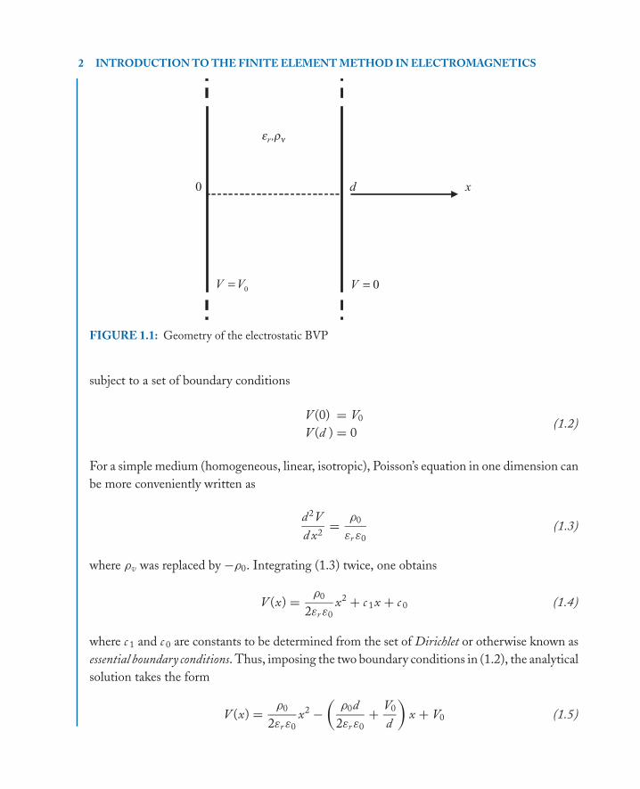
1.2 ELECTROSTATIC BVP AND THE ANALYTICAL SOLUTION
Problem definition: Consider two infinite in extent parallel conducting plates that are positioned
normal to the x-axis and separated by a distance d , as shown in Figure 1.1. One plate is
maintained at a fixed potential V = V0 and the second plate is maintained at V = 0 (ground).
The region between the plates is filled with a nonmagnetic medium having a dielectric constant
εr and a uniform electron volume charge density ρv = −ρ0. Obtain the analytical expressions
for the electric (or electrostatic) potential and the electric field in the region between the two
parallel plates.
Analytical solution: The potential distribution at any point between the two plates is governed
by Poisson’s equation
∇(εr ∇V ) = −ρv
ε0
(1.1)
P1: IML/FFX P2: IML/FFX QC: IML/FFX T1: IML
MOBK021-01 MOBK021-Polycarpou.cls April 29, 2006 19:14
2 INTRODUCTION TO THE FINITE ELEMENT METHOD IN ELECTROMAGNETICS
FIGURE 1.1: Geometry of the electrostatic BVP
subject to a set of boundary conditions
V (0) = V0
V (d ) = 0(1.2)
For a simple medium (homogeneous, linear, isotropic), Poisson’s equation in one dimension can
be more conveniently written as
d 2V
d x2= ρ0
εr ε0
(1.3)
where ρv was replaced by −ρ0. Integrating (1.3) twice, one obtains
V (x) = ρ0
2εr ε0
x2 + c 1x + c 0 (1.4)
where c 1 and c 0 are constants to be determined from the set of Dirichlet or otherwise known as
essential boundary conditions. Thus, imposing the two boundary conditions in (1.2), the analytical
solution takes the form
V (x) = ρ0
2εr ε0
x2 −(
ρ0d
2εr ε0
+ V0
d
)x + V0 (1.5)
P1: IML/FFX P2: IML/FFX QC: IML/FFX T1: IML
MOBK021-01 MOBK021-Polycarpou.cls April 29, 2006 19:14
ONE-DIMENSIONAL BOUNDARY-VALUE PROBLEMS 3
The electric field expression is obtained by taking the negative gradient of the electric
potential
�E(x) = −∇V = −axdV(x)
d x(1.6)
which results in
�E(x) = ax
[V0
d+ ρ0d
2εr ε0
− ρ0x
εr ε0
](1.7)
indicating that the electric field is a function of x-coordinate and is directed along the x-axis. It
is also important to notice here that the electric potential for this particular BVP is a quadratic
function of x whereas the electric field is a linear function of x.
1.3 THE FINITE ELEMENT METHODThe FEM [1–5] is a numerical technique that is used to solve BVPs governed by a differential
equation and a set of boundary conditions. The main idea behind the method is the repre-
sentation of the domain with smaller subdomains called the finite elements. The distribution
of the primary unknown quantity inside an element is interpolated based on the values at the
nodes, provided nodal elements are used, or the values at the edges, in case vector elements are
used. The interpolation or shape functions must be a complete set of polynomials. The accuracy
of the solution depends, among other factors, on the order of these polynomials, which may
be linear, quadratic, or higher order. The numerical solution corresponds to the values of the
primary unknown quantity at the nodes or the edges of the discretized domain. The solution is
obtained after solving a system of linear equations. To form such a linear system of equations,
the governing differential equation and associated boundary conditions must first be converted
to an integro-differential formulation either by minimizing a functional or using a weighted-
residual method such as the Galerkin approach. This integro-differential formulation is applied
to a single element and with the use of proper weight and interpolation functions the respective
element equations are obtained. The assembly of all elements results in a global matrix system
that represents the entire domain of the BVP.
As said in the previous paragraph, there are two methods that are widely used to obtain
the finite element equations: the variational method and the weighted-residual method. The
variational approach requires construction of a functional which represents the energy associated
with the BVP at hand. A functional is a function expressed in an integral form and has arguments
that are functions themselves. Many engineers and scientists refer to a functional as being a
function of functions. A stable or stationary solution to a BVP can be obtained by minimizing or
maximizing the governing functional. Such a solution corresponds to either a minimum point,
a maximum point, or a saddle point. In the vicinity of such a point, the numerical solution is

P1: IML/FFX P2: IML/FFX QC: IML/FFX T1: IML
MOBK021-01 MOBK021-Polycarpou.cls April 29, 2006 19:14
4 INTRODUCTION TO THE FINITE ELEMENT METHOD IN ELECTROMAGNETICS
stable meaning that it is rather insensitive to small variations of dependent parameters. This
translates to a smaller numerical error compared to a solution that corresponds to any other
point. The process of minimizing or maximizing a functional involves taking partial derivatives
of the functional with respect to each of the dependent variables and setting them to zero.
This forms a set of equations that can be discretized with the proper choice of subdomain
interpolation functions to generate the finite element equations.
The second method, which is the one followed in this book, is a weighted-residual method
widely known as the Galerkin method. This method begins by forming a residual directly from
the partial differential equation that is associated with the BVP under study. Simply stated,
this method does not require the use of a functional. The residual is formed by transferring
all terms of the partial differential equation on one side. This residual is then multiplied by a
weight function and integrated over the domain of a single element. This is the reason why the
method is termed as weighted-residual method. If the differential equation is of second order, as
is the case with all the problems considered in this book, it is required that the shape functions
used to interpolate the primary unknown quantity be twice differentiable. This requirement is
weakened by using integration by parts and distributing the second derivative equally between
the weight functions and the interpolation functions. In this way, the associated weight functions
and interpolation functions are required to be only once differentiable. Due to this weakened
requirement, the outlined formulation is also referred to as the weak formulation. In addition, if
the weight functions are chosen from the same set of functions as the interpolation functions,
the underlined weighted-residual method is called Galerkin method.
In this book, we decided to follow the Galerkin approach rather than the variational
approach. The reason stems from the fact that the Galerkin approach is simple and starts directly
from the governing differential equation. Consequently, a beginner will have less difficulty
understand and comprehend the steps involved in the formulation of this method. On the
contrast, variational methods require knowledge of variational principles [6–8] in order for
someone to be able to construct a functional. For some well-known BVPs, the corresponding
functional is often available, but there are cases that it is necessary to construct one using
variational techniques. To avoid the tedious procedure of constructing a functional and the
associated mathematical complexities, it was considered more appropriate to implement the
Galerkin approach instead of the variational approach.
The major steps involved in the application of the Galerkin FEM for the solution of a
BVP are the following:
• Discretize the domain using finite elements.
• Choose proper interpolation functions (otherwise known as shape functions or basis
functions).
P1: IML/FFX P2: IML/FFX QC: IML/FFX T1: IML
MOBK021-01 MOBK021-Polycarpou.cls April 29, 2006 19:14
ONE-DIMENSIONAL BOUNDARY-VALUE PROBLEMS 5
1 2 3 Ne
2 1 3 4 Nn Nn–1
x
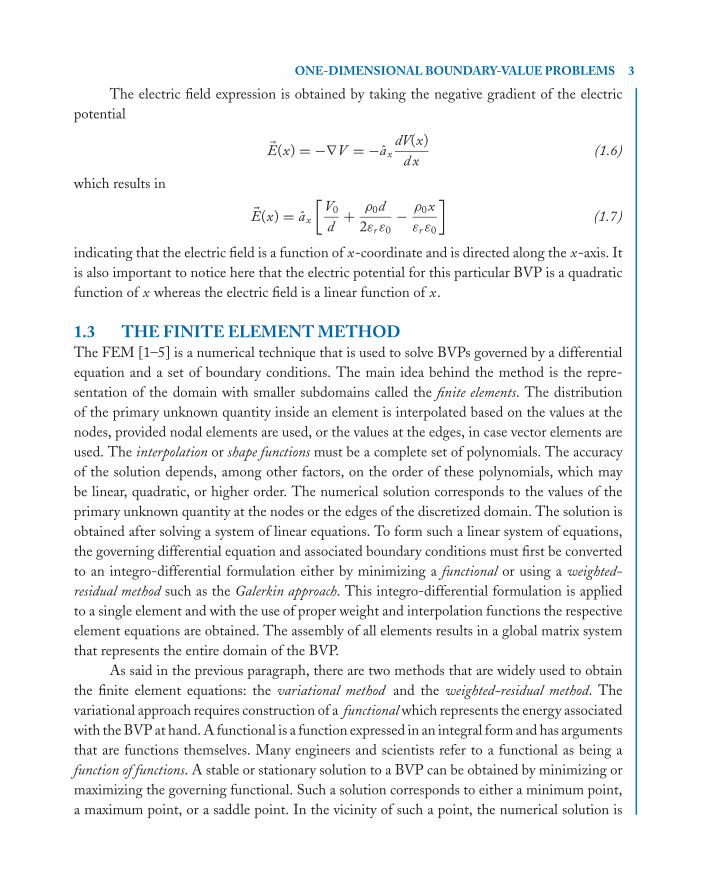
FIGURE 1.2: Discretization of the 1-D domain
• Obtain the corresponding linear equations for a single element by first deriving the
weak formulation of the differential equation subject to a set of boundary conditions.
• Form the global matrix system of equations through the assembly of all elements.
• Impose Dirichlet boundary conditions.
• Solve the linear system of equations using linear algebra techniques.
• Postprocess the results.
These steps will be followed one-by-one in order to solve the electrostatic BVP at hand.
1.4 DOMAIN DISCRETIZATIONThe domain of the problem at hand corresponds to a straight line along the x-axis extending
from x = 0 to x = d . As shown in Figure 1.2, the domain is subdivided into Ne line segments
called the finite elements. These elements constitute the finite element mesh. The element
number is shown circled in the figure. Each element has two nodes; therefore, the total number
of nodes in the domain is Nn = Ne + 1. Depending on the order of shape functions, it may be
necessary to introduce additional nodes inside each element. Such elements are known as higher
order elements. For linear elements, there are only two nodes that are located at the endpoints of
the segment. The finite elements do not have to be of the same length. An element is allowed
to have an arbitrary length to provide the ability to generate a denser mesh near regions where
the solution is expected to have rapid spatial variations. In addition, the discretization of the
domain allows the weak formulation of the problem to be applied to each element separately,
thus allowing us to define distinct element values for material properties and sources. This offers
generality and versatility to the method.
1.5 INTERPOLATION FUNCTIONSThe approximate solution obtained from the weak formulation of the problem over the dis-
cretized domain is represented inside an element by a set of interpolation functions otherwise
known as shape functions. Since the weak formulation of the problem, as it will be outlined in the
following section, contains first-order derivatives of the primary unknown quantity, the chosen
interpolation functions must be continuous within the element and at least once differentiable.
P1: IML/FFX P2: IML/FFX QC: IML/FFX T1: IML
MOBK021-01 MOBK021-Polycarpou.cls April 29, 2006 19:14
6 INTRODUCTION TO THE FINITE ELEMENT METHOD IN ELECTROMAGNETICS
2 e e
1
–1
2 x
2
ex +1
(a) (b)
ξ
1
ex
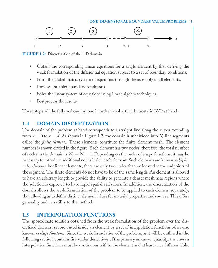
FIGURE 1.3: (a) Element along x-axis. (b) Element along ξ-axis (master element)
The simplest choice is a polynomial of degree one. The use of a polynomial instead of any other
type of function allows for the integrations, which are products of the weak formulation, to be
evaluated more easily. Besides continuity and differentiability, another important requirement is
that these polynomials must be complete. In other words, they must consist of all the lower order
terms. This is essential in order for the solution to be accurately represented by the interpolation
functions inside an element.
Let us now consider a finite element (line segment), as illustrated in Figure 1.3(a). This
element has coordinates xe1 and xe
2, which correspond to local nodes 1 and 2, respectively. The
coordinate transformation
ξ = 2(x − xe1)
xe2 − xe
1
− 1 (1.8)
can be used to transform the element along the x-axis to the master element, shown in
Figure 1.3(b), which resides on the ξ-axis. The ξ-coordinate is also known as the natural
coordinate. As illustrated in the figure, the master element has a fixed position along the natural
coordinate axis. The left node of the element (node 1) maps to ξ = −1 whereas the right node
(node 2) maps to ξ = +1. It is therefore easier for us to integrate a function on the natural
coordinate system rather than on the regular coordinate system. In other words, by mapping
an element onto the natural coordinate axis, the limits of integration involved in the weak
formulation do not change every time a new element is considered. This would be the case if
an integral were to be evaluated for elements residing on the regular coordinate axis. Due to
this observation, it is instructive that interpolation functions be derived based on the master
element rather than the local element.
At any point inside the master element (−1 ≤ ξ ≤ 1), the primary unknown quantity (in
our case the electrostatic potential V ) can be expressed as
V (ξ ) = V e1 N1(ξ ) + V e
2 N2(ξ ) (1.9)
where N1(ξ ), N2(ξ ) are the interpolation functions that correspond to nodes 1 and 2, respectively,
and V e1 , V e
2 are the values of the primary unknown quantity at the two nodes of the element.
Note that the number of interpolation functions used per element is equal to the number of
P1: IML/FFX P2: IML/FFX QC: IML/FFX T1: IML
MOBK021-01 MOBK021-Polycarpou.cls April 29, 2006 19:14
ONE-DIMENSIONAL BOUNDARY-VALUE PROBLEMS 7
1
x–1 +1 –1
+1
x
N1 N2
x–1 +1
V1
eV
2
eV
(a) (b)
(c)
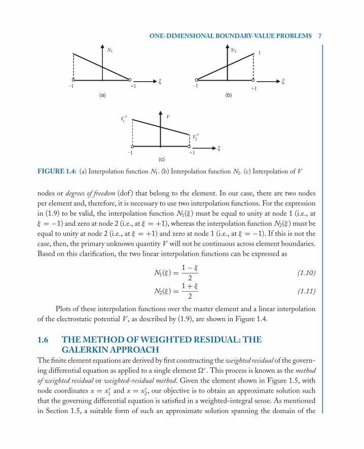
FIGURE 1.4: (a) Interpolation function N1. (b) Interpolation function N2. (c) Interpolation of V
nodes or degrees of freedom (dof ) that belong to the element. In our case, there are two nodes
per element and, therefore, it is necessary to use two interpolation functions. For the expression
in (1.9) to be valid, the interpolation function N1(ξ ) must be equal to unity at node 1 (i.e., at
ξ = −1) and zero at node 2 (i.e., at ξ = +1), whereas the interpolation function N2(ξ ) must be
equal to unity at node 2 (i.e., at ξ = +1) and zero at node 1 (i.e., at ξ = −1). If this is not the
case, then, the primary unknown quantity V will not be continuous across element boundaries.
Based on this clarification, the two linear interpolation functions can be expressed as
N1(ξ ) = 1 − ξ
2(1.10)
N2(ξ ) = 1 + ξ
2(1.11)
Plots of these interpolation functions over the master element and a linear interpolation
of the electrostatic potential V , as described by (1.9), are shown in Figure 1.4.
1.6 THE METHOD OF WEIGHTED RESIDUAL: THEGALERKIN APPROACH
The finite element equations are derived by first constructing the weighted residual of the govern-
ing differential equation as applied to a single element �e . This process is known as the method
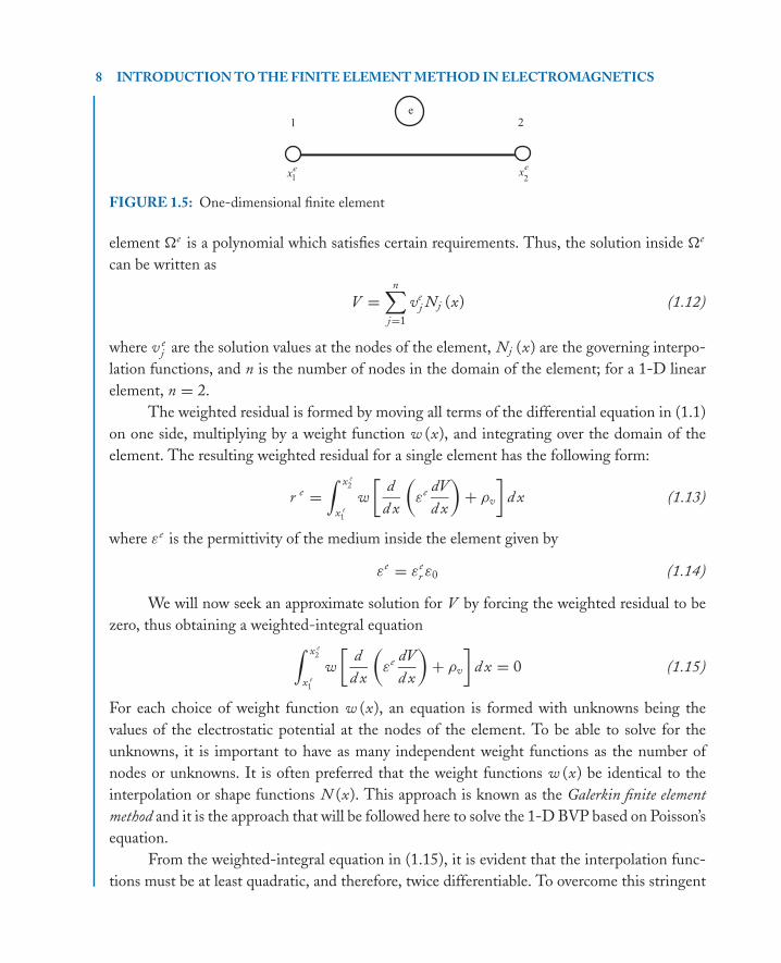
of weighted residual or weighted-residual method. Given the element shown in Figure 1.5, with
node coordinates x = xe1 and x = xe
2, our objective is to obtain an approximate solution such
that the governing differential equation is satisfied in a weighted-integral sense. As mentioned
in Section 1.5, a suitable form of such an approximate solution spanning the domain of the
P1: IML/FFX P2: IML/FFX QC: IML/FFX T1: IML
MOBK021-01 MOBK021-Polycarpou.cls April 29, 2006 19:14
8 INTRODUCTION TO THE FINITE ELEMENT METHOD IN ELECTROMAGNETICS
1 2
1ex
2
ex
e
FIGURE 1.5: One-dimensional finite element
element �e is a polynomial which satisfies certain requirements. Thus, the solution inside �e
can be written as
V =n∑
j=1
vej Nj (x) (1.12)
where v ej are the solution values at the nodes of the element, Nj (x) are the governing interpo-
lation functions, and n is the number of nodes in the domain of the element; for a 1-D linear
element, n = 2.
The weighted residual is formed by moving all terms of the differential equation in (1.1)
on one side, multiplying by a weight function w (x), and integrating over the domain of the
element. The resulting weighted residual for a single element has the following form:
r e =∫ x e
2
x e1
w
[d
d x
(εe dV
d x
)+ ρv
]d x (1.13)
where εe is the permittivity of the medium inside the element given by
εe = εer ε0 (1.14)
We will now seek an approximate solution for V by forcing the weighted residual to be
zero, thus obtaining a weighted-integral equation∫ x e2
x e1
w
[d
d x
(εe dV
d x
)+ ρv
]d x = 0 (1.15)
For each choice of weight function w (x), an equation is formed with unknowns being the
values of the electrostatic potential at the nodes of the element. To be able to solve for the
unknowns, it is important to have as many independent weight functions as the number of
nodes or unknowns. It is often preferred that the weight functions w (x) be identical to the
interpolation or shape functions N (x). This approach is known as the Galerkin finite element
method and it is the approach that will be followed here to solve the 1-D BVP based on Poisson’s
equation.
From the weighted-integral equation in (1.15), it is evident that the interpolation func-
tions must be at least quadratic, and therefore, twice differentiable. To overcome this stringent
P1: IML/FFX P2: IML/FFX QC: IML/FFX T1: IML
MOBK021-01 MOBK021-Polycarpou.cls April 29, 2006 19:14
ONE-DIMENSIONAL BOUNDARY-VALUE PROBLEMS 9
requirement and be able to use linear interpolation functions as well, integration by parts can be
used to trade the double differentiation on V (x) to an evenly distributed single differentiation
on both V (x) and w (x). Integration by parts states that∫ b
a
U dV = U V |ba −
∫ b
a
V dU (1.16)
Using this identity, the first term of the weighted-integral equation can be conveniently written
as ∫ xe2
xe1
wd
d x
(εe dV
d x
)d x =
∫ xe2
xe1
w d
(εe dV
d x
)= w εe dV
d x
∣∣∣∣xe2
xe1
−∫ xe
1
xe1
(dw
d x
)εe
(dV
d x
)d x
(1.17)
Thus, the weak formulation of the governing differential equation can be expressed as∫ xe2
xe1
(dw
d x
)εe
(dV
d x
)d x −
∫ xe2
xe1
w ρv d x − w εe dV
d x
∣∣∣∣xe2
xe1
= 0 (1.18)
The above weak formulation requires that the interpolation functions be at least once differen-
tiable. The last term is evaluated at the two endpoints of the element resulting in
w εe dV
d x
∣∣∣∣xe2
xe1
= w(xe
2
) [εe dV
d x
]x=xe
2
− w(xe
1
) [εe dV
d x
]x=xe
1
(1.19)
From electrostatics [9], it is known that the electric flux density or electric displacement is
defined along the x-axis as
D ex = −εe dV
d x(1.20)
Substituting (1.20) into (1.19), the latter becomes
w εe dV
d x
∣∣∣∣xe2
xe1
= −w(xe
2
)D e
x
(xe
2
) + w(xe
1
)D e
x
(xe
1
)(1.21)
As a result of this observation, the weak form of the differential equation becomes∫ xe2
xe1
(dw
d x
)εe
(dV
d x
)d x −
∫ xe2
xe1
w ρv d x + w(xe
2
)D e
x
(xe
2
) − w(xe
1
)D e
x
(xe
1
) = 0 (1.22)
The finite element equations for a single finite element �e , according to the Galerkin approach,
can be obtained by substituting the approximate solution, given by (1.12), in the weak form of
the differential equation and taking the weight functions as being identical to the interpolation
functions. Thus, for 1-D linear elements, the finite element equations, after we substitute the
P1: IML/FFX P2: IML/FFX QC: IML/FFX T1: IML
MOBK021-01 MOBK021-Polycarpou.cls April 29, 2006 19:14
10 INTRODUCTION TO THE FINITE ELEMENT METHOD IN ELECTROMAGNETICS
approximate solution for n = 2 and the appropriate weight functions, take the following form:∫ xe2
xe1
(dN1
d x
)εe
(2∑
j=1
vej
dN j
d x
)d x =
∫ xe2
xe1
N1ρvd x + N1
(xe
1
)D e
x
(xe
1
) − N1
(xe
2
)D e
x
(xe
2
)∫ xe
2
xe1
(dN2
d x
)εe
(2∑
j=1
vej
dN j
d x
)d x =
∫ xe2
xe1
N2ρvd x + N2
(xe
1
)D e
x
(xe
1
) − N2
(xe
2
)D e
x
(xe
2
) (1.23)
Based on the properties of the interpolation functions introduced in the previous section, it is
deduced that
N1
(xe
1
) = 1
N2
(xe
1
) = 0
N1
(xe
2
) = 0
N2
(xe
2
) = 1
(1.24)
As a result, the finite element equations in (1.23) can be expressed as∫ xe2
xe1
(dN1
d x
)εe
(2∑
j=1
vej
dN j
d x
)d x =
∫ xe2
xe1
N1ρvd x + D ex
(xe
1
)∫ xe
2
xe1
(dN2
d x
)εe
(2∑
j=1
vej
dN j
d x
)d x =
∫ xe2
xe1
N2ρvd x − D ex
(xe
2
) (1.25)
The two algebraic equations in (1.25) can be conveniently written in matrix form[K e
11 K e12
K e21 K e
22
] {v e
1
v e2
}=
{f e1
f e2
}+
{D e
1
−D e2
}(1.26)
where
K ei j =
∫ xe2
xe1
(dNi
d x
)εe
(dN j
d x
)d x (1.27)
and
f ei =
∫ xe2
xe1
Niρvd x (1.28)
for i = 1, 2 and j = 1, 2. The second element right-hand-side vector in (1.26) is denoted by
de; i.e.,
de ={
De1
−De2
}(1.29)
P1: IML/FFX P2: IML/FFX QC: IML/FFX T1: IML
MOBK021-01 MOBK021-Polycarpou.cls April 29, 2006 19:14
ONE-DIMENSIONAL BOUNDARY-VALUE PROBLEMS 11
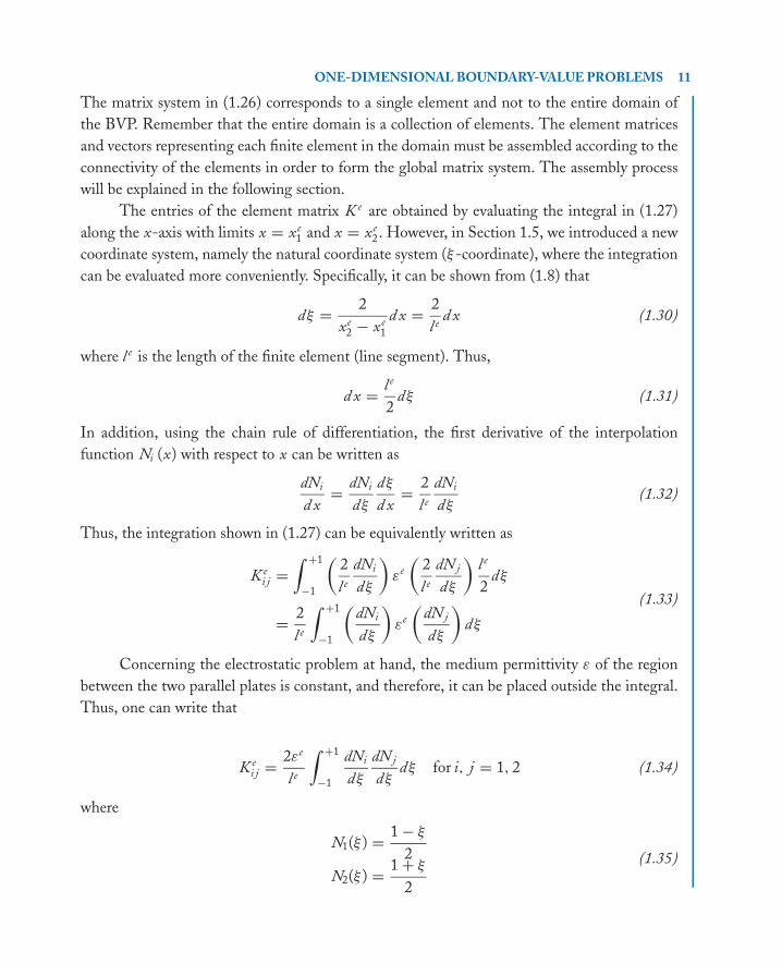
The matrix system in (1.26) corresponds to a single element and not to the entire domain of
the BVP. Remember that the entire domain is a collection of elements. The element matrices
and vectors representing each finite element in the domain must be assembled according to the
connectivity of the elements in order to form the global matrix system. The assembly process
will be explained in the following section.
The entries of the element matrix K e are obtained by evaluating the integral in (1.27)
along the x-axis with limits x = xe1 and x = xe
2. However, in Section 1.5, we introduced a new
coordinate system, namely the natural coordinate system (ξ-coordinate), where the integration
can be evaluated more conveniently. Specifically, it can be shown from (1.8) that
dξ = 2
xe2 − xe
1
d x = 2
l ed x (1.30)
where l e is the length of the finite element (line segment). Thus,
d x = l e
2dξ (1.31)
In addition, using the chain rule of differentiation, the first derivative of the interpolation
function Ni (x) with respect to x can be written as
dNi
d x= dNi
dξ
dξ
d x= 2
l e
dNi
dξ(1.32)
Thus, the integration shown in (1.27) can be equivalently written as
K ei j =
∫ +1
−1
(2
l e
dNi
dξ
)εe
(2
l e
dN j
dξ
)l e
2dξ
= 2
l e
∫ +1
−1
(dNi
dξ
)εe
(dN j
dξ
)dξ
(1.33)
Concerning the electrostatic problem at hand, the medium permittivity ε of the region
between the two parallel plates is constant, and therefore, it can be placed outside the integral.
Thus, one can write that
K ei j = 2εe
l e
∫ +1
−1
dNi
dξ
dN j
dξdξ for i, j = 1, 2 (1.34)
where
N1(ξ ) = 1 − ξ
2
N2(ξ ) = 1 + ξ
2
(1.35)

P1: IML/FFX P2: IML/FFX QC: IML/FFX T1: IML
MOBK021-01 MOBK021-Polycarpou.cls April 29, 2006 19:14
12 INTRODUCTION TO THE FINITE ELEMENT METHOD IN ELECTROMAGNETICS
From the above definition of the two linear interpolation functions with respect to ξ , it is evident
that
dN1
dξ= −1
2(1.36)
and
dN2
dξ= +1
2(1.37)
As a result, the corresponding entries of the element matrix K e are given by
K e = εe
l e
[+1 −1
−1 +1
](1.38)
In a similar way, the entries of the element right-hand-side vector f e can be evaluated using
(1.28). For the electrostatic BVP at hand, the volume charge density ρv was assumed constant
and equal to −ρ0. Thus, using the coordinate transformation from the regular coordinate system
(x-axis) to the natural coordinate system (ξ-axis), the integral in (1.28) can be more conveniently
written as
f ei = − l e ρ0
2
∫ +1
−1
Ni (ξ )dξ (1.39)
Substituting (1.35) into (1.39), one obtains
f e1 = − l e ρ0
2
∫ +1
−1
(1 − ξ
2
)dξ = − l e ρ0
4
[ξ − ξ 2
2
]+1
−1
= − l e ρ0
2(1.40)
f e2 = − l e ρ0
2
∫ +1
−1
(1 + ξ
2
)dξ = − l e ρ0
4
[ξ + ξ 2
2
]+1
−1
= − l e ρ0
2(1.41)
Therefore, vector f e can be expressed as
f e = − l e ρ0
2
{1
1
}(1.42)
The governing matrix system for a single element is given by
εe
l e
[+1 −1
−1 +1
] {v e
1
v e2
}= − l e ρ0
2
{1
1
}+
{D e
1
−D e2
}(1.43)
P1: IML/FFX P2: IML/FFX QC: IML/FFX T1: IML
MOBK021-01 MOBK021-Polycarpou.cls April 29, 2006 19:14
ONE-DIMENSIONAL BOUNDARY-VALUE PROBLEMS 13
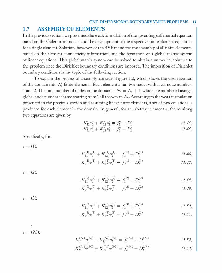
1.7 ASSEMBLY OF ELEMENTSIn the previous section, we presented the weak formulation of the governing differential equation
based on the Galerkin approach and the development of the respective finite element equations
for a single element. Solution, however, of the BVP mandates the assembly of all finite elements,
based on the element connectivity information, and the formation of a global matrix system
of linear equations. This global matrix system can be solved to obtain a numerical solution to
the problem once the Dirichlet boundary conditions are imposed. The imposition of Dirichlet
boundary conditions is the topic of the following section.
To explain the process of assembly, consider Figure 1.2, which shows the discretization
of the domain into Ne finite elements. Each element e has two nodes with local node numbers
1 and 2. The total number of nodes in the domain is Nn = Ne + 1, which are numbered using a
global node number scheme starting from 1 all the way to Nn. According to the weak formulation
presented in the previous section and assuming linear finite elements, a set of two equations is
produced for each element in the domain. In general, for an arbitrary element e , the resulting
two equations are given by
K e11ve
1 + K e12ve
2 = f e1 + De
1 (1.44)
K e21ve
1 + K e22ve
2 = f e2 − De
2 (1.45)
Specifically, for
e = (1):
K(1)
11 v(1)1 + K
(1)12 v
(1)2 = f
(1)1 + D
(1)1 (1.46)
K(1)
21 v(1)1 + K
(1)22 v
(1)2 = f
(1)2 − D
(1)2 (1.47)
e = (2):
K(2)
11 v(2)1 + K
(2)12 v
(2)2 = f
(2)1 + D
(2)1 (1.48)
K(2)
21 v(2)1 + K
(2)22 v
(2)2 = f
(2)2 − D
(2)2 (1.49)
e = (3):
K(3)
11 v(3)1 + K
(3)12 v
(3)2 = f
(3)1 + D
(3)1 (1.50)
K(3)
21 v(3)1 + K
(3)22 v
(3)2 = f
(3)2 − D
(3)2 (1.51)
...
e = (Ne ):
K(Ne )
11 v(Ne )1 + K
(Ne )12 v
(Ne )2 = f
(Ne )1 + D
(Ne )1 (1.52)
K(Ne )
21 v(Ne )1 + K
(Ne )22 v
(Ne )2 = f
(Ne )2 − D
(Ne )2 (1.53)
P1: IML/FFX P2: IML/FFX QC: IML/FFX T1: IML
MOBK021-01 MOBK021-Polycarpou.cls April 29, 2006 19:14
14 INTRODUCTION TO THE FINITE ELEMENT METHOD IN ELECTROMAGNETICS
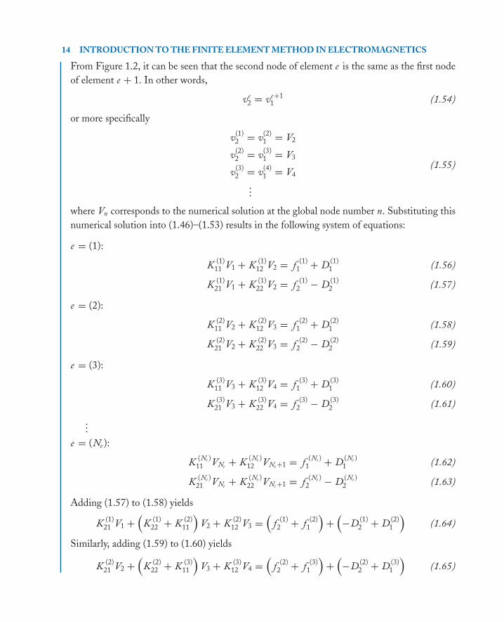
From Figure 1.2, it can be seen that the second node of element e is the same as the first node
of element e + 1. In other words,
ve2 = ve+1
1 (1.54)
or more specifically
v(1)2 = v
(2)1 = V2
v(2)2 = v
(3)1 = V3
v(3)2 = v
(4)1 = V4
...
(1.55)
where Vn corresponds to the numerical solution at the global node number n. Substituting this
numerical solution into (1.46)–(1.53) results in the following system of equations:
e = (1):
K(1)
11 V1 + K(1)
12 V2 = f(1)
1 + D(1)1 (1.56)
K(1)
21 V1 + K(1)
22 V2 = f(1)
2 − D(1)2 (1.57)
e = (2):
K(2)
11 V2 + K(2)
12 V3 = f(2)
1 + D(2)1 (1.58)
K(2)
21 V2 + K(2)
22 V3 = f(2)
2 − D(2)2 (1.59)
e = (3):
K(3)
11 V3 + K(3)
12 V4 = f(3)
1 + D(3)1 (1.60)
K(3)
21 V3 + K(3)
22 V4 = f(3)
2 − D(3)2 (1.61)
...
e = (Ne ):
K(Ne )
11 VNe+ K
(Ne )12 VNe +1 = f
(Ne )1 + D
(Ne )1 (1.62)
K(Ne )
21 VNe+ K
(Ne )22 VNe +1 = f
(Ne )2 − D
(Ne )2 (1.63)
Adding (1.57) to (1.58) yields
K(1)
21 V1 +(
K(1)
22 + K(2)
11
)V2 + K
(2)12 V3 =
(f
(1)2 + f
(2)1
)+
(−D
(1)2 + D
(2)1
)(1.64)
Similarly, adding (1.59) to (1.60) yields
K(2)
21 V2 +(
K(2)
22 + K(3)
11
)V3 + K
(3)12 V4 =
(f
(2)2 + f
(3)1
)+
(−D
(2)2 + D
(3)1
)(1.65)
P1: IML/FFX P2: IML/FFX QC: IML/FFX T1: IML
MOBK021-01 MOBK021-Polycarpou.cls April 29, 2006 19:14
ONE-DIMENSIONAL BOUNDARY-VALUE PROBLEMS 15
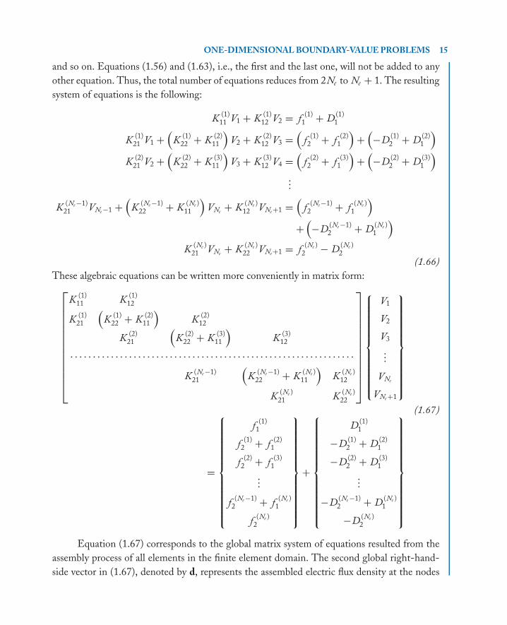
and so on. Equations (1.56) and (1.63), i.e., the first and the last one, will not be added to any
other equation. Thus, the total number of equations reduces from 2Ne to Ne + 1. The resulting
system of equations is the following:
K(1)
11 V1 + K(1)
12 V2 = f(1)
1 + D(1)1
K(1)
21 V1 +(
K(1)
22 + K(2)
11
)V2 + K
(2)12 V3 =
(f
(1)2 + f
(2)1
)+
(−D
(1)2 + D
(2)1
)K
(2)21 V2 +
(K
(2)22 + K
(3)11
)V3 + K
(3)12 V4 =
(f
(2)2 + f
(3)1
)+
(−D
(2)2 + D
(3)1
)...
K (Ne −1)21 VNe −1 +
(K
(Ne −1)22 + K
(Ne )11
)VNe
+ K(Ne )
12 VNe +1 =(
f(Ne −1)
2 + f(Ne )
1
)+
(−D
(Ne −1)2 + D
(Ne )1
)K
(Ne )21 VNe
+ K(Ne )
22 VNe +1 = f(Ne )
2 − D(Ne )2
(1.66)
These algebraic equations can be written more conveniently in matrix form:⎡⎢⎢⎢⎢⎢⎢⎢⎢⎢⎢⎢⎢⎣
K(1)
11 K(1)
12
K(1)
21
(K
(1)22 + K
(2)11
)K
(2)12
K(2)
21
(K
(2)22 + K
(3)11
)K
(3)12
. . . . . . . . . . . . . . . . . . . . . . . . . . . . . . . . . . . . . . . . . . . . . . . . . . . . . . . . . . . . . . .
K(Ne −1)
21
(K
(Ne −1)22 + K
(Ne )11
)K
(Ne )12
K(Ne )
21 K(Ne )
22
⎤⎥⎥⎥⎥⎥⎥⎥⎥⎥⎥⎥⎥⎦
⎧⎪⎪⎪⎪⎪⎪⎪⎪⎪⎪⎪⎨⎪⎪⎪⎪⎪⎪⎪⎪⎪⎪⎪⎩
V1
V2
V3
...
VNe
VNe +1
⎫⎪⎪⎪⎪⎪⎪⎪⎪⎪⎪⎪⎬⎪⎪⎪⎪⎪⎪⎪⎪⎪⎪⎪⎭
=
⎧⎪⎪⎪⎪⎪⎪⎪⎪⎪⎪⎪⎪⎨⎪⎪⎪⎪⎪⎪⎪⎪⎪⎪⎪⎪⎩
f(1)
1
f(1)
2 + f(2)
1
f(2)
2 + f(3)
1
...
f(Ne −1)
2 + f(Ne )
1
f(Ne )
2
⎫⎪⎪⎪⎪⎪⎪⎪⎪⎪⎪⎪⎪⎬⎪⎪⎪⎪⎪⎪⎪⎪⎪⎪⎪⎪⎭+
⎧⎪⎪⎪⎪⎪⎪⎪⎪⎪⎪⎪⎪⎨⎪⎪⎪⎪⎪⎪⎪⎪⎪⎪⎪⎪⎩
D(1)1
−D(1)2 + D
(2)1
−D(2)2 + D
(3)1
...
−D(Ne −1)2 + D
(Ne )1
−D(Ne )2
⎫⎪⎪⎪⎪⎪⎪⎪⎪⎪⎪⎪⎪⎬⎪⎪⎪⎪⎪⎪⎪⎪⎪⎪⎪⎪⎭
(1.67)
Equation (1.67) corresponds to the global matrix system of equations resulted from the
assembly process of all elements in the finite element domain. The second global right-hand-
side vector in (1.67), denoted by d, represents the assembled electric flux density at the nodes
P1: IML/FFX P2: IML/FFX QC: IML/FFX T1: IML
MOBK021-01 MOBK021-Polycarpou.cls April 29, 2006 19:14
16 INTRODUCTION TO THE FINITE ELEMENT METHOD IN ELECTROMAGNETICS
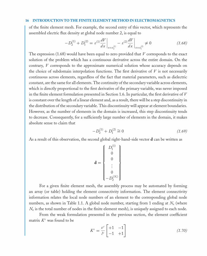
of the finite element mesh. For example, the second entry of this vector, which represents the
assembled electric flux density at global node number 2, is equal to
−D(1)2 + D
(2)1 = ε(1) dV
d x
∣∣∣∣x=x
(1)2
− ε(2) dV
d x
∣∣∣∣x=x
(2)1
�= 0 (1.68)
The expression (1.68) would have been equal to zero provided that V corresponds to the exact
solution of the problem which has a continuous derivative across the entire domain. On the
contrary, V corresponds to the approximate numerical solution whose accuracy depends on
the choice of subdomain interpolation functions. The first derivative of V is not necessarily
continuous across elements, regardless of the fact that material parameters, such as dielectric
constant, are the same for all elements. The continuity of the secondary variable across elements,
which is directly proportional to the first derivative of the primary variable, was never imposed
in the finite element formulation presented in Section 1.6. In particular, the first derivative of V
is constant over the length of a linear element and, as a result, there will be a step discontinuity in
the distribution of the secondary variable. This discontinuity will appear at element boundaries.
However, as the number of elements in the domain is increased, this step discontinuity tends
to decrease. Consequently, for a sufficiently large number of elements in the domain, it makes
absolute sense to claim that
−D (1)2 + D
(2)1
∼= 0 (1.69)
As a result of this observation, the second global right-hand-side vector d can be written as
d =
⎧⎪⎪⎪⎪⎪⎪⎪⎪⎨⎪⎪⎪⎪⎪⎪⎪⎪⎩
D(1)1
0
0...
0
−D (Ne )2
⎫⎪⎪⎪⎪⎪⎪⎪⎪⎬⎪⎪⎪⎪⎪⎪⎪⎪⎭For a given finite element mesh, the assembly process may be automated by forming
an array (or table) holding the element connectivity information. The element connectivity
information relates the local node numbers of an element to the corresponding global node
numbers, as shown in Table 1.1. A global node number, starting from 1 ending at Nn (where
Nn is the total number of nodes in the finite element mesh), is uniquely assigned to each node.
From the weak formulation presented in the previous section, the element coefficient
matrix K e was found to be
K e = εe
l e
[+1 −1
−1 +1
](1.70)

P1: IML/FFX P2: IML/FFX QC: IML/FFX T1: IML
MOBK021-01 MOBK021-Polycarpou.cls April 29, 2006 19:14
ONE-DIMENSIONAL BOUNDARY-VALUE PROBLEMS 17
TABLE 1.1: Element connectivity information
ELEMENT LOCAL NODE 1 LOCAL NODE 2
1 1 2
2 2 3
3 3 4
......
...
Ne Nn − 1 Nn
This element coefficient matrix must be mapped, according to the element connectivity infor-
mation, to the global coefficient matrix with dimensions Nn × Nn. Here the word “mapping”
means adding the entries of the element coefficient matrix to the corresponding entries of the
global coefficient matrix. Note that the global coefficient matrix K must be initialized to the
zero matrix before we begin the assembly process. Therefore, according to Table 1.1, entry K e11
of element 2 maps to entry K22 of the global matrix; entry K e12 of element 2 maps to entry
K23 of the global matrix, and so on. To illustrate the assembly process, consider an example
where we have only three elements in the domain, i.e., Ne = 3 and Nn = 4. As a result, the
dimensions of the global matrix is 4 × 4 and can be formed by adding the contribution of each
element coefficient matrix to an initialized-to-zero global K matrix. Thus,
K = ε(1)
l (1)
⎡⎢⎢⎢⎣+1 −1 0 0
−1 +1 0 0
0 0 0 0
0 0 0 0
⎤⎥⎥⎥⎦ + ε(2)
l (2)
⎡⎢⎢⎢⎣0 0 0 0
0 +1 −1 0
0 −1 +1 0
0 0 0 0
⎤⎥⎥⎥⎦ + ε(3)
l (3)
⎡⎢⎢⎢⎣0 0 0 0
0 0 0 0
0 0 +1 −1
0 0 −1 +1
⎤⎥⎥⎥⎦ (1.71)
which is equal to
K =
⎡⎢⎢⎢⎢⎢⎢⎢⎢⎢⎢⎣
ε(1)
l (1)−ε(1)
l (1)0 0
−ε(1)
l (1)
(ε(1)
l (1)+ ε(2)
l (2)
)−ε(2)
l (2)0
0 −ε(2)
l (2)
(ε(2)
l (2)+ ε(3)
l (3)
)−ε(3)
l (3)
0 0 −ε(3)
l (3)
ε(3)
l (3)
⎤⎥⎥⎥⎥⎥⎥⎥⎥⎥⎥⎦(1.72)
P1: IML/FFX P2: IML/FFX QC: IML/FFX T1: IML
MOBK021-01 MOBK021-Polycarpou.cls April 29, 2006 19:14
18 INTRODUCTION TO THE FINITE ELEMENT METHOD IN ELECTROMAGNETICS
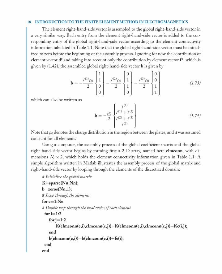
The element right-hand-side vector is assembled to the global right-hand-side vector in
a very similar way. Each entry from the element right-hand-side vector is added to the cor-
responding entry of the global right-hand-side vector according to the element connectivity
information tabulated in Table 1.1. Note that the global right-hand-side vector must be initial-
ized to zero before the beginning of the assembly process. Ignoring for now the contribution of
element vector de and taking into account only the contribution by element vector f e, which is
given by (1.42), the assembled global right-hand-side vector b is given by
b = − l (1)ρ0
2
⎧⎪⎪⎪⎨⎪⎪⎪⎩1
1
0
0
⎫⎪⎪⎪⎬⎪⎪⎪⎭ − l (2)ρ0
2
⎧⎪⎪⎪⎨⎪⎪⎪⎩0
1
1
0
⎫⎪⎪⎪⎬⎪⎪⎪⎭ − l (3)ρ0
2
⎧⎪⎪⎪⎨⎪⎪⎪⎩0
0
1
1
⎫⎪⎪⎪⎬⎪⎪⎪⎭ (1.73)
which can also be written as
b = −ρ0
2
⎧⎪⎪⎪⎨⎪⎪⎪⎩l (1)
l (1) + l (2)
l (2) + l (3)
l (3)
⎫⎪⎪⎪⎬⎪⎪⎪⎭ (1.74)
Note that ρ0 denotes the charge distribution in the region between the plates, and it was assumed
constant for all elements.
Using a computer, the assembly process of the global coefficient matrix and the global
right-hand-side vector begins by forming first a 2-D array, named here elmconn, with di-
mensions Ne × 2, which holds the element connectivity information given in Table 1.1. A
simple algorithm written in Matlab illustrates the assembly process of the global matrix and
right-hand-side vector by looping through the elements of the discretized domain:
# Initialize the global matrix
K=sparse(Nn,Nn);
b=zeros(Nn,1);
# Loop through the elements
for e=1:Ne
# Double loop through the local nodes of each element
for i=1:2
for j=1:2
K(elmconn(e,i),elmconn(e,j))=K(elmconn(e,i),elmconn(e,j))+Ke(i,j);
end
b(elmconn(e,i))=b(elmconn(e,i))+fe(i);
end
end
P1: IML/FFX P2: IML/FFX QC: IML/FFX T1: IML
MOBK021-01 MOBK021-Polycarpou.cls April 29, 2006 19:14
ONE-DIMENSIONAL BOUNDARY-VALUE PROBLEMS 19
The names of the variables used are self-explanatory, e.g., elmconn stands for the array holding
the element connectivity information. In addition, for the filling of the global coefficient
matrix, the Matlab command sparse was used in order to save on computer memory by avoiding
storing the zero entries. Note that the majority of entries in the global coefficient matrix will
be zero after the completion of the assembly process. We call such a matrix a sparse matrix.
The sparsity of the global coefficient matrix is attributed to the subdomain nature of the shape
functions. In other words, a given shape function, which corresponds to a specific node, is
nonzero only inside the elements where this node belongs to. For the remaining elements
in the discretized domain, this specific shape function is zero and, therefore, there is no
interaction between the specific node and the associated nodes of those elements. As a result,
the corresponding entries of the global coefficient matrix will be zero.
1.8 IMPOSITION OF BOUNDARY CONDITIONSThis section outlines the procedure used to impose boundary conditions on the set of linear
equations obtained from the weak formulation of the governing differential equation. Prior
to imposing boundary conditions, the global matrix system is singular and, thus, cannot be
solved to obtain a unique solution. A nonsingular matrix system is obtained after imposing
the boundary conditions associated with a given BVP. The two types of boundary conditions
that are discussed in this section are the Dirichlet or essential boundary conditions and the mixed
boundary conditions. The Dirichlet boundary conditions involve only the primary unknown
variable whereas the mixed boundary conditions involve both the primary unknown variable
and its derivative. Another type of boundary conditions is the Neumann boundary conditions
which can be considered as a special case of the mixed boundary conditions.
1.8.1 Dirichlet Boundary Conditions
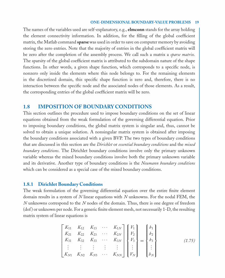
The weak formulation of the governing differential equation over the entire finite element
domain results in a system of N linear equations with N unknowns. For the nodal FEM, the
N unknowns correspond to the N nodes of the domain. Thus, there is one degree of freedom
(dof ) or unknown per node. For a generic finite element mesh, not necessarily 1-D, the resulting
matrix system of linear equations is⎡⎢⎢⎢⎢⎢⎢⎣K11 K12 K13 · · · K1N
K21 K22 K23 · · · K2N
K31 K32 K33 · · · K3N
......
......
...
KN1 KN2 KN3 · · · KNN
⎤⎥⎥⎥⎥⎥⎥⎦
⎧⎪⎪⎪⎪⎪⎪⎨⎪⎪⎪⎪⎪⎪⎩
V1
V2
V3
...
VN
⎫⎪⎪⎪⎪⎪⎪⎬⎪⎪⎪⎪⎪⎪⎭=
⎧⎪⎪⎪⎪⎪⎪⎨⎪⎪⎪⎪⎪⎪⎩
b1
b2
b3
...
b N
⎫⎪⎪⎪⎪⎪⎪⎬⎪⎪⎪⎪⎪⎪⎭(1.75)
P1: IML/FFX P2: IML/FFX QC: IML/FFX T1: IML
MOBK021-01 MOBK021-Polycarpou.cls April 29, 2006 19:14
20 INTRODUCTION TO THE FINITE ELEMENT METHOD IN ELECTROMAGNETICS
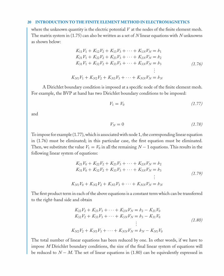
where the unknown quantity is the electric potential V at the nodes of the finite element mesh.
The matrix system in (1.75) can also be written as a set of N linear equations with N unknowns
as shown below:
K11V1 + K12V2 + K13V3 + · · · + K1N VN = b1
K21V1 + K22V2 + K23V3 + · · · + K2N VN = b2
K31V1 + K32V2 + K33V3 + · · · + K3N VN = b3
...
KN1V1 + KN2V2 + KN3V3 + · · · + KNN VN = b N
(1.76)
A Dirichlet boundary condition is imposed at a specific node of the finite element mesh.
For example, the BVP at hand has two Dirichlet boundary conditions to be imposed:
V1 = V0 (1.77)
and
VN = 0 (1.78)
To impose for example (1.77), which is associated with node 1, the corresponding linear equation
in (1.76) must be eliminated; in this particular case, the first equation must be eliminated.
Then, we substitute the value V1 = V0 in all the remaining N − 1 equations. This results in the
following linear system of equations:
K21V0 + K22V2 + K23V3 + · · · + K2N VN = b2
K31V0 + K32V2 + K33V3 + · · · + K3N VN = b3
...
KN1V0 + KN2V2 + KN3V3 + · · · + KNN VN = b N
(1.79)
The first product term in each of the above equations is a constant term which can be transferred
to the right-hand side and obtain
K22V2 + K23V3 + · · · + K2N VN = b2 − K21V0
K32V2 + K33V3 + · · · + K3N VN = b3 − K31V0
...
KN2V2 + KN3V3 + · · · + KNN VN = b N − KN1V0
(1.80)
The total number of linear equations has been reduced by one. In other words, if we have to
impose M Dirichlet boundary conditions, the size of the final linear system of equations will
be reduced to N − M. The set of linear equations in (1.80) can be equivalently expressed in

P1: IML/FFX P2: IML/FFX QC: IML/FFX T1: IML
MOBK021-01 MOBK021-Polycarpou.cls April 29, 2006 19:14
ONE-DIMENSIONAL BOUNDARY-VALUE PROBLEMS 21
matrix form as ⎡⎢⎢⎢⎢⎣K22 K23 · · · K2N
K32 K33 · · · K3N
...... · · · ...
KN2 KN3 · · · KNN
⎤⎥⎥⎥⎥⎦⎧⎪⎪⎪⎪⎨⎪⎪⎪⎪⎩
V2
V3
...
VN
⎫⎪⎪⎪⎪⎬⎪⎪⎪⎪⎭ =
⎧⎪⎪⎪⎪⎨⎪⎪⎪⎪⎩b2 − K21V0
b3 − K31V0
...
b N − KN1V0
⎫⎪⎪⎪⎪⎬⎪⎪⎪⎪⎭ (1.81)
Comparing the global matrix system in (1.81) with the global matrix system in (1.75),
which corresponds to the problem before imposing the first Dirichlet boundary condition, it is
obvious that the first row of the matrix and right-hand-side vector, as well as the first column of
the matrix, were eliminated. The remaining entries of the right-hand-side vector were updated
according to
bi = bi − Ki1V0 for i = 2, 3, . . . , N (1.82)
In general, to impose a Dirichlet boundary condition at a given node n, let us say
Vn = V0 (1.83)
the nth row of the system matrix, the nth row of the right-hand-side vector, and the nth row
of the unknown vector, as well as the nth column of the system matrix must be eliminated,
whereas the remaining entries of the right-hand-side vector must be updated according to
bi = bi − KinV0 for i = 1, 2, . . . , N; i �= n (1.84)
After eliminating a given row, all the rows underneath must be shifted upward by one position.
Similarly, after eliminating a given column, all the columns on the right must be shifted toward
the left by one position.
Once the matrix system is solved, only N − M unknowns will be determined; the values
of the primary unknown quantity at the remaining M nodes are known from the set of Dirichlet
boundary conditions. This method of imposing Dirichlet boundary conditions is known as the
Method of Elimination because the algebraic equation that corresponds to the global node at
which the Dirichlet boundary condition is imposed must be eliminated, thus reducing the size
of the governing matrix system by one.
From a programming point of view, it is more convenient to number the global nodes of
the finite element mesh in such a way that the nodes which correspond to Dirichlet boundary
conditions appear last. Thus, using the method of elimination in imposing Dirichlet boundary
conditions, it is not necessary every time we delete a row to have to shift the bottom rows
upward. The same argument applies to columns as well. This will save computational time and
make programming simpler and more straightforward.
P1: IML/FFX P2: IML/FFX QC: IML/FFX T1: IML
MOBK021-01 MOBK021-Polycarpou.cls April 29, 2006 19:14
22 INTRODUCTION TO THE FINITE ELEMENT METHOD IN ELECTROMAGNETICS
1.8.2 Mixed Boundary Conditions
A mixed boundary condition, unlike a Dirichlet or Neumann boundary condition, involves the
variable of the quantity under study and its derivative. A generic form of a mixed boundary
condition can be expressed as
εdV
d x+ αV = β (1.85)
where α and β are constants. For a Neumann boundary condition, i.e., dV/d x = 0 at a given
x-coordinate, constants α and β are set to zero. As it will be shown in Chapter 2, a first-order
absorbing boundary condition (ABC), which is used in scattering and radiation problems to
truncate the unbounded free space, is a form of a mixed boundary condition. To impose this
mixed boundary condition at an exterior node, let us say the rightmost node of the domain with
global number N, we need to remind ourselves that the global right-hand-side vector b is a
superposition of two other global vectors namely f and d where
d =
⎧⎪⎪⎪⎪⎪⎪⎨⎪⎪⎪⎪⎪⎪⎩
D (1)1
0...
0
−D (Ne )2
⎫⎪⎪⎪⎪⎪⎪⎬⎪⎪⎪⎪⎪⎪⎭=
⎧⎪⎪⎪⎪⎪⎪⎪⎪⎪⎪⎨⎪⎪⎪⎪⎪⎪⎪⎪⎪⎪⎩
−ε(1)dV
d x
∣∣∣∣x=x
(1)1
0...
0
ε(Ne )dV
d x
∣∣∣∣x=x
(Ne )2
⎫⎪⎪⎪⎪⎪⎪⎪⎪⎪⎪⎬⎪⎪⎪⎪⎪⎪⎪⎪⎪⎪⎭(1.86)
To impose the mixed boundary condition given by (1.85) at the rightmost node of the finite
element mesh, we must replace the last entry of vector d by
ε(Ne ) dV
d x
∣∣∣∣x=x
(Ne )2
= β − αVN (1.87)
Note that VN is the unknown potential at the Nth node of the domain. The term αVN is
therefore transferred to the left-hand side whereas β stays at the last entry position of vector d.
Transferring αVN to the left-hand side of the matrix system is equivalent to adding constant α
to the KNN entry of the global coefficient matrix. A detailed explanation on how a first-order
ABC is implemented in a 2-D scattering problem will be provided in Chapter 2.
1.9 FINITE ELEMENT SOLUTION OF THE ELECTROSTATICBOUNDARY-VALUE PROBLEM
After going through the major steps of the FEM, we are now in the position to use this powerful
numerical method to solve the electrostatic BVP at hand. Remember that the objective is to
P1: IML/FFX P2: IML/FFX QC: IML/FFX T1: IML
MOBK021-01 MOBK021-Polycarpou.cls April 29, 2006 19:14
ONE-DIMENSIONAL BOUNDARY-VALUE PROBLEMS 23
x
1 2 3 4
x x2=2 x3=4 x4=6 x5=8
3 4 3 4 5 1 2
=0
(cm)(cm)
1
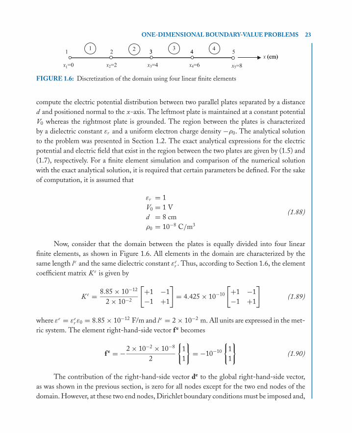
FIGURE 1.6: Discretization of the domain using four linear finite elements
compute the electric potential distribution between two parallel plates separated by a distance
d and positioned normal to the x-axis. The leftmost plate is maintained at a constant potential
V0 whereas the rightmost plate is grounded. The region between the plates is characterized
by a dielectric constant εr and a uniform electron charge density −ρ0. The analytical solution
to the problem was presented in Section 1.2. The exact analytical expressions for the electric
potential and electric field that exist in the region between the two plates are given by (1.5) and
(1.7), respectively. For a finite element simulation and comparison of the numerical solution
with the exact analytical solution, it is required that certain parameters be defined. For the sake
of computation, it is assumed that
εr = 1
V0 = 1 V
d = 8 cm
ρ0 = 10−8 C/m3
(1.88)
Now, consider that the domain between the plates is equally divided into four linear
finite elements, as shown in Figure 1.6. All elements in the domain are characterized by the
same length l e and the same dielectric constant εer . Thus, according to Section 1.6, the element
coefficient matrix K e is given by
K e = 8.85 × 10⁻¹²
2 × 10⁻²
[+1 −1
−1 +1
]= 4.425 × 10⁻¹⁰
[+1 −1
−1 +1
](1.89)
where εe = εer ε0 = 8.85 × 10⁻¹² F/m and l e = 2 × 10⁻² m. All units are expressed in the met-
ric system. The element right-hand-side vector f e becomes
f e = −2 × 10−2 × 10−8
2
{1
1
}= −10−10
{1
1
}(1.90)
The contribution of the right-hand-side vector de to the global right-hand-side vector,
as was shown in the previous section, is zero for all nodes except for the two end nodes of the
domain. However, at these two end nodes, Dirichlet boundary conditions must be imposed and,

P1: IML/FFX P2: IML/FFX QC: IML/FFX T1: IML
MOBK021-01 MOBK021-Polycarpou.cls April 29, 2006 19:14
24 INTRODUCTION TO THE FINITE ELEMENT METHOD IN ELECTROMAGNETICS
therefore, the contribution by vector de is effectively discarded. Thus, based on the assembly
process presented in Section 1.7, the global matrix system for the finite element mesh, depicted
in Figure 1.6, becomes
4.425 × 10⁻¹⁰
⎡⎢⎢⎢⎢⎢⎣1 −1 0 0 0
−1 2 −1 0 0
0 −1 2 −1 0
0 0 −1 2 −1
0 0 0 −1 1
⎤⎥⎥⎥⎥⎥⎦
⎧⎪⎪⎪⎪⎪⎨⎪⎪⎪⎪⎪⎩
V1
V2
V3
V4
V5
⎫⎪⎪⎪⎪⎪⎬⎪⎪⎪⎪⎪⎭= −10−10
⎧⎪⎪⎪⎪⎪⎨⎪⎪⎪⎪⎪⎩
1
2
2
2
1
⎫⎪⎪⎪⎪⎪⎬⎪⎪⎪⎪⎪⎭(1.91)
Dividing both sides by 4.425 × 10⁻¹⁰, the matrix system can be equivalently written as⎡⎢⎢⎢⎢⎢⎣1 −1 0 0 0
−1 2 −1 0 0
0 −1 2 −1 0
0 0 −1 2 −1
0 0 0 −1 1
⎤⎥⎥⎥⎥⎥⎦
⎧⎪⎪⎪⎪⎪⎨⎪⎪⎪⎪⎪⎩
V1
V2
V3
V4
V5
⎫⎪⎪⎪⎪⎪⎬⎪⎪⎪⎪⎪⎭=
⎧⎪⎪⎪⎪⎪⎨⎪⎪⎪⎪⎪⎩
−0.2259887
−0.4519774
−0.4519774
−0.4519774
−0.2259887
⎫⎪⎪⎪⎪⎪⎬⎪⎪⎪⎪⎪⎭(1.92)
Imposing the Dirichlet boundary condition V = 1 at node 1 eliminates the entire first
row, including the first row of the right-hand-side vector, and the first column of the coefficient
matrix. Once this is done, the right-hand-side vector must be updated according to (1.82), thus
resulting in the following reduced matrix system:⎡⎢⎢⎢⎣2 −1 0 0
−1 2 −1 0
0 −1 2 −1
0 0 −1 1
⎤⎥⎥⎥⎦⎧⎪⎪⎪⎨⎪⎪⎪⎩
V2
V3
V4
V5
⎫⎪⎪⎪⎬⎪⎪⎪⎭ =
⎧⎪⎪⎪⎨⎪⎪⎪⎩0.5480226
−0.4519774
−0.4519774
−0.2259887
⎫⎪⎪⎪⎬⎪⎪⎪⎭ (1.93)
The second boundary condition V = 0 at node 5 is imposed by eliminating the entire
last row of the matrix system and the last column of the coefficient matrix. Updating the
right-hand-side vector is needless since V5 = 0. Thus, the final global matrix system becomes⎡⎢⎣ 2 −1 0
−1 2 −1
0 −1 2
⎤⎥⎦⎧⎪⎨⎪⎩
V2
V3
V4
⎫⎪⎬⎪⎭ =
⎧⎪⎨⎪⎩0.5480226
−0.4519774
−0.4519774
⎫⎪⎬⎪⎭ (1.94)
This global matrix system can be solved using several techniques most of which can
be found in common linear algebra books. One such technique is Cramer’s rule, which is also
P1: IML/FFX P2: IML/FFX QC: IML/FFX T1: IML
MOBK021-01 MOBK021-Polycarpou.cls April 29, 2006 19:14
ONE-DIMENSIONAL BOUNDARY-VALUE PROBLEMS 25
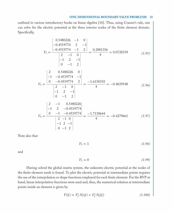
outlined in various introductory books on linear algebra [10]. Thus, using Cramer’s rule, one
can solve for the electric potential at the three interior nodes of the finite element domain.
Specifically,
V2 =
∣∣∣∣∣∣∣∣∣0.5480226 −1 0
−0.4519774 2 −1
−0.4519774 −1 2
∣∣∣∣∣∣∣∣∣∣∣∣∣∣∣∣∣∣2 −1 0
−1 2 −1
0 −1 2
∣∣∣∣∣∣∣∣∣
= 0.2881356
4= 0.0720339 (1.95)
V3 =
∣∣∣∣∣∣∣∣∣2 0.5480226 0
−1 −0.4519774 −1
0 −0.4519774 2
∣∣∣∣∣∣∣∣∣∣∣∣∣∣∣∣∣∣2 −1 0
−1 2 −1
0 −1 2
∣∣∣∣∣∣∣∣∣
= −1.6158192
4= −0.4039548 (1.96)
V4 =
∣∣∣∣∣∣∣∣∣2 −1 0.5480226
−1 2 −0.4519774
0 −1 −0.4519774
∣∣∣∣∣∣∣∣∣∣∣∣∣∣∣∣∣∣2 −1 0
−1 2 −1
0 −1 2
∣∣∣∣∣∣∣∣∣
= −1.7118644
4= −0.4279661 (1.97)
Note also that
V1 = 1 (1.98)
and
V5 = 0 (1.99)
Having solved the global matrix system, the unknown electric potential at the nodes of
the finite element mesh is found. To plot the electric potential at intermediate points requires
the use of the interpolation or shape functions employed for each finite element. For the BVP at
hand, linear interpolation functions were used and, thus, the numerical solution at intermediate
points inside an element is given by
V (ξ ) = V e1 N1(ξ ) + V e
2 N2(ξ ) (1.100)
P1: IML/FFX P2: IML/FFX QC: IML/FFX T1: IML
MOBK021-01 MOBK021-Polycarpou.cls April 29, 2006 19:14
26 INTRODUCTION TO THE FINITE ELEMENT METHOD IN ELECTROMAGNETICS
where
N1(ξ ) = 1 − ξ
2
N2(ξ ) = 1 + ξ
2
(1.101)
and
ξ = 2(x − xe
1
)xe
2 − xe1
− 1 (1.102)
Substituting (1.102) into (1.101) yields
N1(x) = xe2 − x
xe2 − xe
1
N2(x) = x − xe1
xe2 − xe
1
(1.103)
Consequently, the electric potential at any point inside an element can be written as
V (x) = V e1
(xe
2 − x
xe2 − xe
1
)+ V e
2
(x − xe
1
xe2 − xe
1
)(1.104)
where V e1 and V e
2 are the values of the electric potential at the two end nodes of the element.
The electric field at any point inside an element is computed by taking the negative gradient of
the electric potential given by (1.104)
�E = −∇V (1.105)
which is equivalent to
�E = −axdV (x)
d x(1.106)
since the electric potential is only a function of the x-coordinate. Applying (1.106) on (1.104)
yields
�E = −ax
[− V e
1
xe2 − xe
1
+ V e2
xe2 − xe
1
]= ax
[V e
1 − V e2
xe2 − xe
1
]= ax
(V e
1 − V e2
)l e
(1.107)
where l e = xe2 − xe
1 is the length of the element. Unlike the electric potential, which is contin-
uous across element boundaries, the electric field is discontinuous. In addition, due to the use
of linear interpolation functions, the electric field (which is proportional to the gradient of the
P1: IML/FFX P2: IML/FFX QC: IML/FFX T1: IML
MOBK021-01 MOBK021-Polycarpou.cls April 29, 2006 19:14
ONE-DIMENSIONAL BOUNDARY-VALUE PROBLEMS 27
0.0 0.01 0.02 0.03 0.04 0.05 0.06 0.07 0.08
Distance (m)
–0.4
–0.2
0.0
0.2
0.4
0.6
0.8
1.0
Ele
ctri
cp
ote
nti
al(V
)FEM
Exact
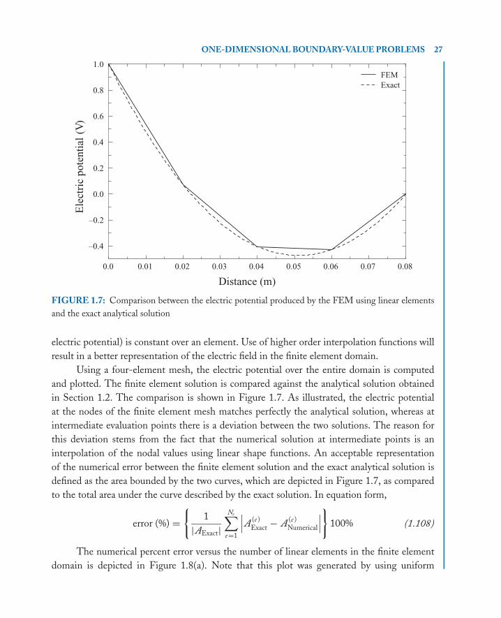
FIGURE 1.7: Comparison between the electric potential produced by the FEM using linear elements
and the exact analytical solution
electric potential) is constant over an element. Use of higher order interpolation functions will
result in a better representation of the electric field in the finite element domain.
Using a four-element mesh, the electric potential over the entire domain is computed
and plotted. The finite element solution is compared against the analytical solution obtained
in Section 1.2. The comparison is shown in Figure 1.7. As illustrated, the electric potential
at the nodes of the finite element mesh matches perfectly the analytical solution, whereas at
intermediate evaluation points there is a deviation between the two solutions. The reason for
this deviation stems from the fact that the numerical solution at intermediate points is an
interpolation of the nodal values using linear shape functions. An acceptable representation
of the numerical error between the finite element solution and the exact analytical solution is
defined as the area bounded by the two curves, which are depicted in Figure 1.7, as compared
to the total area under the curve described by the exact solution. In equation form,
error (%) ={
1
|AExact|Ne∑
e=1
∣∣∣A(e )Exact − A
(e )Numerical
∣∣∣} 100% (1.108)
The numerical percent error versus the number of linear elements in the finite element
domain is depicted in Figure 1.8(a). Note that this plot was generated by using uniform

P1: IML/FFX P2: IML/FFX QC: IML/FFX T1: IML
MOBK021-01 MOBK021-Polycarpou.cls April 29, 2006 19:14
28 INTRODUCTION TO THE FINITE ELEMENT METHOD IN ELECTROMAGNETICS
5 10 15 20 25 30 35 40 45 5010
–1
100
101
102
Err
or (
%)
(a)
5 10 15 20 25 30 35 40 45 5010
–5
10–4
10–3
10–2
Number of elements
L 2-n
orm
(b)
Number of elements
FIGURE 1.8: (a) Numerical percent error based on area. (b) Error based on the L2-norm definition
discretization, meaning that all elements (line segments) had exactly the same length. From
this figure, it is observed that by doubling the number of elements, which is equivalent to
reducing the length of the elements to half, the percent error in the numerical solution, as
compared to the exact analytical solution, is reduced by a factor of 4. This can be clearly seen
from Table 1.2, which shows the numerical value of the computed percent error as a function
of the number of linear elements.
TABLE 1.2: Numerical error as a function of the number of linear elements
NUMBER OF LINEAR NUMERICAL PERCENT ERROR BASED ON THE
ELEMENTS ERROR L2 NORM
5 23.4862 7.5 × 10⁻³
10 5.8716 1.9 × 10⁻³
15 2.6096 8.3 × 10⁻⁴
20 1.4679 4.7 × 10⁻⁴
25 0.9394 3.0 × 10⁻⁴
30 0.6524 2.1 × 10⁻⁴
35 0.4793 1.5 × 10⁻⁴
40 0.3670 1.2 × 10⁻⁴
45 0.2900 9.2 × 10⁻⁵
50 0.2349 7.5 × 10⁻⁵
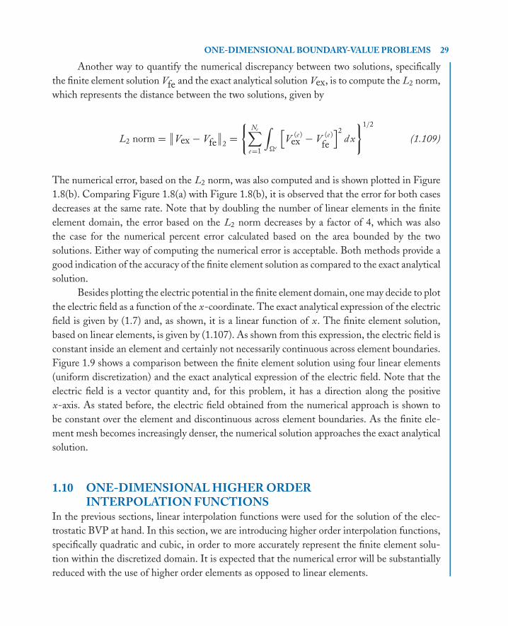
P1: IML/FFX P2: IML/FFX QC: IML/FFX T1: IML
MOBK021-01 MOBK021-Polycarpou.cls April 29, 2006 19:14
ONE-DIMENSIONAL BOUNDARY-VALUE PROBLEMS 29
Another way to quantify the numerical discrepancy between two solutions, specifically
the finite element solution Vfe and the exact analytical solution Vex, is to compute the L2 norm,
which represents the distance between the two solutions, given by
L2 norm = ∥∥Vex − Vfe
∥∥2
={
Ne∑e=1
∫�e
[V
(e )ex − V
(e )
fe
]2
d x
}1/2
(1.109)
The numerical error, based on the L2 norm, was also computed and is shown plotted in Figure
1.8(b). Comparing Figure 1.8(a) with Figure 1.8(b), it is observed that the error for both cases
decreases at the same rate. Note that by doubling the number of linear elements in the finite
element domain, the error based on the L2 norm decreases by a factor of 4, which was also
the case for the numerical percent error calculated based on the area bounded by the two
solutions. Either way of computing the numerical error is acceptable. Both methods provide a
good indication of the accuracy of the finite element solution as compared to the exact analytical
solution.
Besides plotting the electric potential in the finite element domain, one may decide to plot
the electric field as a function of the x-coordinate. The exact analytical expression of the electric
field is given by (1.7) and, as shown, it is a linear function of x. The finite element solution,
based on linear elements, is given by (1.107). As shown from this expression, the electric field is
constant inside an element and certainly not necessarily continuous across element boundaries.
Figure 1.9 shows a comparison between the finite element solution using four linear elements
(uniform discretization) and the exact analytical expression of the electric field. Note that the
electric field is a vector quantity and, for this problem, it has a direction along the positive
x-axis. As stated before, the electric field obtained from the numerical approach is shown to
be constant over the element and discontinuous across element boundaries. As the finite ele-
ment mesh becomes increasingly denser, the numerical solution approaches the exact analytical
solution.
1.10 ONE-DIMENSIONAL HIGHER ORDERINTERPOLATION FUNCTIONS
In the previous sections, linear interpolation functions were used for the solution of the elec-
trostatic BVP at hand. In this section, we are introducing higher order interpolation functions,
specifically quadratic and cubic, in order to more accurately represent the finite element solu-
tion within the discretized domain. It is expected that the numerical error will be substantially
reduced with the use of higher order elements as opposed to linear elements.
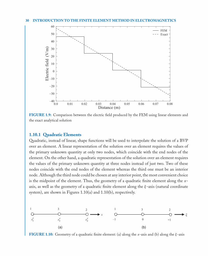
P1: IML/FFX P2: IML/FFX QC: IML/FFX T1: IML
MOBK021-01 MOBK021-Polycarpou.cls April 29, 2006 19:14
30 INTRODUCTION TO THE FINITE ELEMENT METHOD IN ELECTROMAGNETICS
0.0 0.01 0.02 0.03 0.04 0.05 0.06 0.07 0.08
Distance (m)
–40
–30
–20
–10
0
10
20
30
40
50
60
Ele
ctri
cfi
eld
(V/m
)
FEM
Exact
FIGURE 1.9: Comparison between the electric field produced by the FEM using linear elements and
the exact analytical solution
1.10.1 Quadratic Elements
Quadratic, instead of linear, shape functions will be used to interpolate the solution of a BVP
over an element. A linear representation of the solution over an element requires the values of
the primary unknown quantity at only two nodes, which coincide with the end nodes of the
element. On the other hand, a quadratic representation of the solution over an element requires
the values of the primary unknown quantity at three nodes instead of just two. Two of these
nodes coincide with the end nodes of the element whereas the third one must be an interior
node. Although the third node could be chosen at any interior point, the most convenient choice
is the midpoint of the element. Thus, the geometry of a quadratic finite element along the x-
axis, as well as the geometry of a quadratic finite element along the ξ-axis (natural coordinate
system), are shown in Figures 1.10(a) and 1.10(b), respectively.
1 3 2
1ex
x x
(a) (b)
–1 +10
1 2 3
3ex 2
ex
FIGURE 1.10: Geometry of a quadratic finite element: (a) along the x-axis and (b) along the ξ-axis
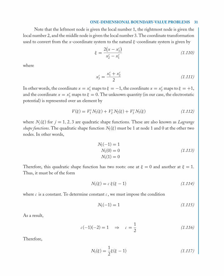
P1: IML/FFX P2: IML/FFX QC: IML/FFX T1: IML
MOBK021-01 MOBK021-Polycarpou.cls April 29, 2006 19:14
ONE-DIMENSIONAL BOUNDARY-VALUE PROBLEMS 31
Note that the leftmost node is given the local number 1, the rightmost node is given the
local number 2, and the middle node is given the local number 3. The coordinate transformation
used to convert from the x-coordinate system to the natural ξ-coordinate system is given by
ξ = 2(x − xe
3
)xe
2 − xe1
(1.110)
where
xe3 = xe
1 + xe2
2(1.111)
In other words, the coordinate x = xe1 maps to ξ = −1, the coordinate x = xe
2 maps to ξ = +1,
and the coordinate x = xe3 maps to ξ = 0. The unknown quantity (in our case, the electrostatic
potential) is represented over an element by
V (ξ ) = V e1 N1(ξ ) + V e
2 N2(ξ ) + V e3 N3(ξ ) (1.112)
where Nj (ξ ) for j = 1, 2, 3 are quadratic shape functions. These are also known as Lagrange
shape functions. The quadratic shape function N1(ξ ) must be 1 at node 1 and 0 at the other two
nodes. In other words,
N1(−1) = 1
N1(0) = 0
N1(1) = 0
(1.113)
Therefore, this quadratic shape function has two roots: one at ξ = 0 and another at ξ = 1.
Thus, it must be of the form
N1(ξ ) = c ξ (ξ − 1) (1.114)
where c is a constant. To determine constant c , we must impose the condition
N1(−1) = 1 (1.115)
As a result,
c (−1)(−2) = 1 ⇒ c = 1
2(1.116)
Therefore,
N1(ξ ) = 1
2ξ (ξ − 1) (1.117)
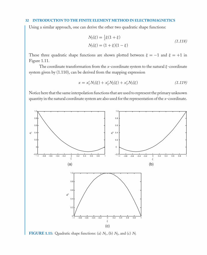
P1: IML/FFX P2: IML/FFX QC: IML/FFX T1: IML
MOBK021-01 MOBK021-Polycarpou.cls April 29, 2006 19:14
32 INTRODUCTION TO THE FINITE ELEMENT METHOD IN ELECTROMAGNETICS
Using a similar approach, one can derive the other two quadratic shape functions:
N2(ξ ) = 12ξ (1 + ξ )
N3(ξ ) = (1 + ξ )(1 − ξ )(1.118)
These three quadratic shape functions are shown plotted between ξ = −1 and ξ = +1 in
Figure 1.11.
The coordinate transformation from the x-coordinate system to the natural ξ-coordinate
system given by (1.110), can be derived from the mapping expression
x = xe1 N1(ξ ) + xe
2 N2(ξ ) + xe3 N3(ξ ) (1.119)
Notice here that the same interpolation functions that are used to represent the primary unknown
quantity in the natural coordinate system are also used for the representation of the x-coordinate.
–1 –0.8 –0.6 –0.4 –0.2 0 0.2 0.4 0.6 0.8 1–0.2
0
0.2
0.4
0.6
0.8
1.0
(a)
0 0.2 0.4 0.6 0.8 1
0
0.2
0.4
0.6
0.8
1.0
(b)
N1
N2
0 0.2 0.4 0.6 0.8 10
0.2
0.4
0.6
0.8
1.0
(c)
N3
–1 –0.8 –0.6 –0.4 –0.2–0.2
–1 –0.8 –0.6 –0.4 –0.2
x
x
x
FIGURE 1.11: Quadratic shape functions: (a) N1, (b) N2, and (c) N3
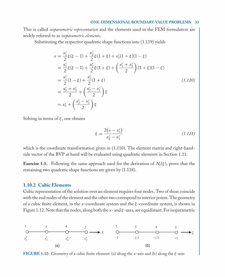
P1: IML/FFX P2: IML/FFX QC: IML/FFX T1: IML
MOBK021-01 MOBK021-Polycarpou.cls April 29, 2006 19:14
ONE-DIMENSIONAL BOUNDARY-VALUE PROBLEMS 33
This is called isoparametric representation and the elements used in the FEM formulation are
widely referred to as isoparametric elements.
Substituting the respective quadratic shape functions into (1.119) yields
x = xe1
2ξ (ξ − 1) + xe
2
2ξ (1 + ξ ) + xe
3(1 + ξ )(1 − ξ )
= xe1
2ξ (ξ − 1) + xe
2
2ξ (1 + ξ ) +
(xe
1 + xe2
2
)(1 + ξ )(1 − ξ )
= xe1
2(1 − ξ ) + xe
2
2(1 + ξ ) (1.120)
= xe1 + xe
2
2+
(xe
2 − xe1
2
)ξ
= xe3 +
(xe
2 − xe1
2
)ξ
Solving in terms of ξ , one obtains
ξ = 2(x − xe
3
)xe
2 − xe1
(1.121)
which is the coordinate transformation given in (1.110). The element matrix and right-hand-
side vector of the BVP at hand will be evaluated using quadratic elements in Section 1.11.
Exercise 1.1. Following the same approach used for the derivation of N1(ξ ), prove that the
remaining two quadratic shape functions are given by (1.118).
1.10.2 Cubic Elements
Cubic representation of the solution over an element requires four nodes. Two of these coincide
with the end nodes of the element and the other two correspond to interior points. The geometry
of a cubic finite element, in the x-coordinate system and the ξ-coordinate system, is shown in
Figure 1.12. Note that the nodes, along both the x- and ξ-axes, are equidistant. For isoparametric
1 3 2
1ex
x
4 4
–1/3 +1/3 3ex
4ex
2ex
(a) (b)
1 2
x3
–1 +1
FIGURE 1.12: Geometry of a cubic finite element: (a) along the x-axis and (b) along the ξ-axis
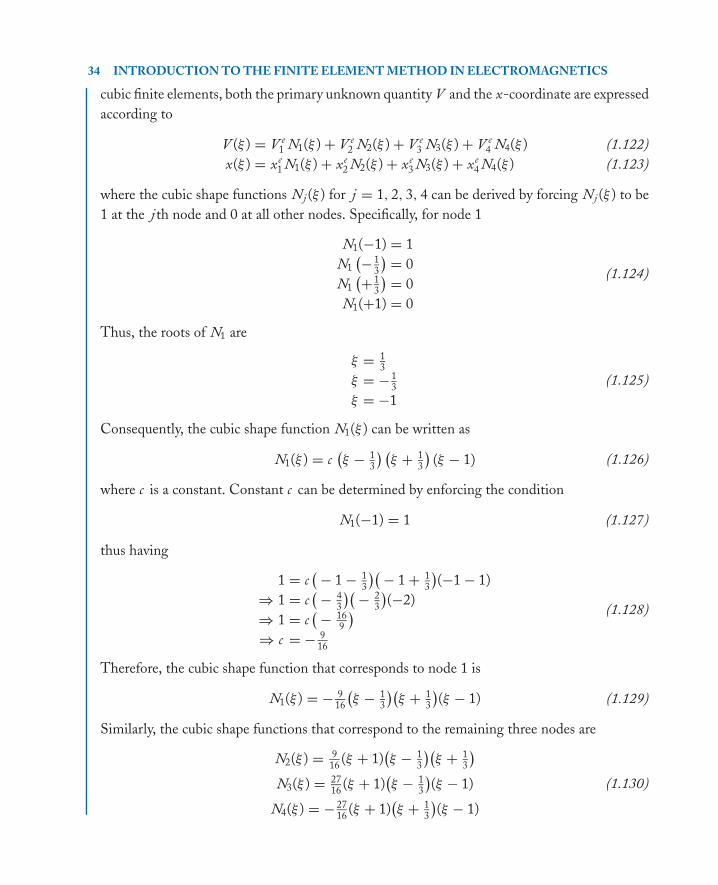
P1: IML/FFX P2: IML/FFX QC: IML/FFX T1: IML
MOBK021-01 MOBK021-Polycarpou.cls April 29, 2006 19:14
34 INTRODUCTION TO THE FINITE ELEMENT METHOD IN ELECTROMAGNETICS
cubic finite elements, both the primary unknown quantity V and the x-coordinate are expressed
according to
V (ξ ) = V e1 N1(ξ ) + V e
2 N2(ξ ) + V e3 N3(ξ ) + V e
4 N4(ξ ) (1.122)
x(ξ ) = xe1 N1(ξ ) + xe
2 N2(ξ ) + xe3 N3(ξ ) + xe
4 N4(ξ ) (1.123)
where the cubic shape functions Nj (ξ ) for j = 1, 2, 3, 4 can be derived by forcing Nj (ξ ) to be
1 at the j th node and 0 at all other nodes. Specifically, for node 1
N1(−1) = 1
N1
(− 13
) = 0
N1
(+ 13
) = 0
N1(+1) = 0
(1.124)
Thus, the roots of N1 are
ξ = 13
ξ = − 13
ξ = −1
(1.125)
Consequently, the cubic shape function N1(ξ ) can be written as
N1(ξ ) = c(ξ − 1
3
) (ξ + 1
3
)(ξ − 1) (1.126)
where c is a constant. Constant c can be determined by enforcing the condition
N1(−1) = 1 (1.127)
thus having
1 = c( − 1 − 1
3
)( − 1 + 13
)(−1 − 1)
⇒ 1 = c( − 4
3
)( − 23
)(−2)
⇒ 1 = c( − 16
9
)⇒ c = − 9
16
(1.128)
Therefore, the cubic shape function that corresponds to node 1 is
N1(ξ ) = − 916
(ξ − 1
3
)(ξ + 1
3
)(ξ − 1) (1.129)
Similarly, the cubic shape functions that correspond to the remaining three nodes are
N2(ξ ) = 916
(ξ + 1)(ξ − 1
3
)(ξ + 1
3
)N3(ξ ) = 27
16(ξ + 1)
(ξ − 1
3
)(ξ − 1)
N4(ξ ) = − 2716
(ξ + 1)(ξ + 1
3
)(ξ − 1)
(1.130)
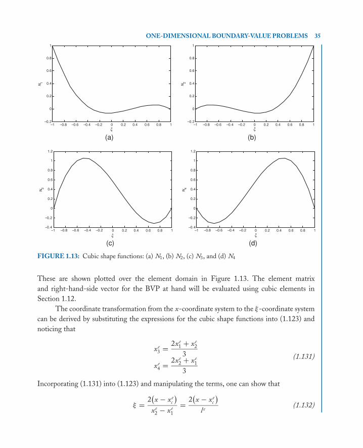
P1: IML/FFX P2: IML/FFX QC: IML/FFX T1: IML
MOBK021-01 MOBK021-Polycarpou.cls April 29, 2006 19:14
ONE-DIMENSIONAL BOUNDARY-VALUE PROBLEMS 35
–1 –0.8 –0.6 –0.4 –0.2 0 0.2 0.4 0.6 0.8 1–0.2
0
0.2
0.4
0.6
0.8
1
(a)
0 0.2 0.4 0.6 0.8 1
0
0.2
0.4
0.6
0.8
1
(b)
0 0.2 0.4 0.6 0.8 1
0
0.2
0.4
0.6
0.8
1
1.2
(c)
0 0.2 0.4 0.6 0.8 1
0
0.2
0.4
0.6
0.8
1
1.2
(d)
N1
N2
N3
N4
–1 –0.8 –0.6 –0.4 –0.2–0.2
–1 –0.8 –0.6 –0.4 –0.2–0.4
–0.2
–1 –0.8 –0.6 –0.4 –0.2–0.4
–0.2
x x
xx
FIGURE 1.13: Cubic shape functions: (a) N1, (b) N2, (c) N3, and (d) N4
These are shown plotted over the element domain in Figure 1.13. The element matrix
and right-hand-side vector for the BVP at hand will be evaluated using cubic elements in
Section 1.12.
The coordinate transformation from the x-coordinate system to the ξ-coordinate system
can be derived by substituting the expressions for the cubic shape functions into (1.123) and
noticing that
xe3 = 2xe
1 + xe2
3
xe4 = 2xe
2 + xe1
3
(1.131)
Incorporating (1.131) into (1.123) and manipulating the terms, one can show that
ξ = 2(x − xe
c
)xe
2 − xe1
= 2(x − xe
c
)l e
(1.132)
P1: IML/FFX P2: IML/FFX QC: IML/FFX T1: IML
MOBK021-01 MOBK021-Polycarpou.cls April 29, 2006 19:14
36 INTRODUCTION TO THE FINITE ELEMENT METHOD IN ELECTROMAGNETICS
where xec is the x-coordinate of the midpoint of the element given by
xec = xe
1 + xe2
2(1.133)
Exercise 1.2. Following the same approach used for the derivation of N1(ξ ), prove that the
remaining three cubic shape functions are given by (1.130).
Exercise 1.3. Using isoparametric cubic elements, show that the coordinate transformation
from the x-coordinate system to the ξ-coordinate system is governed by (1.132).
1.11 ELEMENT MATRIX AND RIGHT-HAND-SIDE VECTORUSING QUADRATIC ELEMENTS
According to the weak formulation presented in Section 1.6, the entries of the element coeffi-
cient matrix and right-hand-side vector are given by
K ei j =
∫ xe2
xe1
(dNi
d x
)εe
(dN j
d x
)d x for i, j = 1, 2, 3 (1.134)
and
f ei =
∫ xe2
xe1
Niρvd x for i = 1, 2, 3 (1.135)
Note that the global right-hand-side vector d does not contribute to the global matrix system
because the only nonzero entries of this vector belong to the first and the last rows. These will
eventually be discarded after imposing the two Dirichlet boundary conditions at the end nodes
of the domain. To obtain the entries of the element coefficient matrix K e , the integral in (1.134)
must be evaluated either analytically or numerically. Using quadratic elements, it was shown
that the expression that maps the x-coordinate to the ξ-coordinate system is given by
ξ = 2(x − xe
3
)xe
2 − xe1
(1.136)
Taking the derivative with respect to x yields
dξ = 2
xe2 − xe
1
d x = 2
l ed x (1.137)
P1: IML/FFX P2: IML/FFX QC: IML/FFX T1: IML
MOBK021-01 MOBK021-Polycarpou.cls April 29, 2006 19:14
ONE-DIMENSIONAL BOUNDARY-VALUE PROBLEMS 37
Thus,
d x = l e
2dξ (1.138)
In addition, using the chain rule of differentiation
dNi
d x= dNi
dξ
dξ
d x= 2
l e
dNi
dξ(1.139)
As a result, the integral in (1.134) can be equivalently expressed in terms of the natural coordinate
instead of the x-coordinate. Doing this, the limits of integration remain always the same for
all elements in the domain, i.e., from −1 to +1. Thus, after the coordinate transformation has
taken place, the integral that is used in the evaluation of the entries of the element coefficient
matrix takes the form
K ei j =
∫ +1
−1
2
l e
dNi
dξεe 2
l e
dN j
dξ
l e
2dξ
= 2εe
l e
∫ +1
−1
(dNi
dξ
) (dN j
dξ
)dξ for i, j = 1, 2, 3
(1.140)
where
N1(ξ ) = 12ξ (ξ − 1)
N2(ξ ) = 12ξ (1 + ξ )
N3(ξ ) = (1 + ξ )(1 − ξ )
(1.141)
Differentiating these three quadratic shape functions with respect to the natural coordinate ξ
yields
dN1
dξ= ξ − 1
2
dN2
dξ= ξ + 1
2
dN3
dξ= −2ξ
(1.142)
Substituting in (1.140) for i = j = 1, the entry K e11 becomes
K e11 = 2εe
l e
∫ +1
−1
(ξ − 1
2
)2
dξ = 7εe
3l e(1.143)

P1: IML/FFX P2: IML/FFX QC: IML/FFX T1: IML
MOBK021-01 MOBK021-Polycarpou.cls April 29, 2006 19:14
38 INTRODUCTION TO THE FINITE ELEMENT METHOD IN ELECTROMAGNETICS
Similarly,
K e12 = K e
21 = εe
3l e
K e13 = K e
31 = −2εe
3l e
K e22 = 7εe
3l e
K e23 = K e
32 = −8εe
3l e
K e33 = 16εe
3l e
(1.144)
Thus, the element coefficient matrix is a 3 × 3 symmetric square matrix given by
K e = εe
3l e
⎡⎢⎣ 7 1 −8
1 7 −8
−8 −8 16
⎤⎥⎦ (1.145)
The element right-hand-side vector is a 3 × 1 vector whose entries are obtained by
evaluating the following integral:
f ei = − l e ρ0
2
∫ +1
−1
Ni (ξ )dξ for i = 1, 2, 3 (1.146)
where ρv was replaced by −ρ0, which is the uniform electron charge density between the two
parallel plates. Substituting the shape functions Ni (ξ ) for i = 1, 2, 3 in (1.146) and evaluating
the corresponding integral, one can obtain analytically the entries of the element vector f e:
f e1 = − l e ρ0
2
∫ +1
−1
1
2ξ (ξ − 1) dξ = − l e ρ0
6
f e2 = − l e ρ0
2
∫ +1
−1
1
2ξ (1 + ξ ) dξ = − l e ρ0
6
f e3 = − l e ρ0
2
∫ +1
−1
(1 + ξ ) (1 − ξ ) dξ = −2l e ρ0
3
(1.147)
As a result, the element right-hand-side vector for quadratic nodal finite elements is given by
f e = − l e ρ0
6
⎧⎪⎨⎪⎩1
1
4
⎫⎪⎬⎪⎭ (1.148)
Exercise 1.4. Using quadratic elements, show that the element coefficient matrix is given by
(1.145).
P1: IML/FFX P2: IML/FFX QC: IML/FFX T1: IML
MOBK021-01 MOBK021-Polycarpou.cls April 29, 2006 19:14
ONE-DIMENSIONAL BOUNDARY-VALUE PROBLEMS 39
1.12 ELEMENT MATRIX AND RIGHT-HAND-SIDE VECTORUSING CUBIC ELEMENTS
The procedure used to derive the element coefficient matrix and right-hand-side vector of the
differential equation at hand is identical to the one used for quadratic elements but certainly a bit
more involved. Symbolic math packages, such as Maple, can be used to analytically obtain the
entries of the element coefficient matrix and right-hand-side vector, thus avoiding unnecessary
mathematical complexities by hand. It can be shown that the governing element coefficient
matrix and right-hand-side vector for cubic elements are given by
K e = εe
40l e
⎡⎢⎢⎢⎣148 −13 −189 54
−13 148 54 −189
−189 54 432 −297
54 −189 −297 432
⎤⎥⎥⎥⎦ (1.149)
f e = − l e ρ0
8
⎧⎪⎪⎪⎨⎪⎪⎪⎩1
1
3
3
⎫⎪⎪⎪⎬⎪⎪⎪⎭ (1.150)
Exercise 1.5. Follow the same formulation presented in Section 1.11 to show that the element
coefficient matrix and right-hand-side vector for cubic elements are given by (1.149) and (1.150),
respectively. To avoid the evaluation of complicated integrals by hand, it is recommended that
the symbolic math package called Maple be utilized.
1.13 POSTPROCESSING OF THE SOLUTION:QUADRATIC ELEMENTS
In the context of FEM, a BVP is represented by a set of independent linear equations that
can be solved numerically, using linear algebra techniques, to obtain the values of the unknown
quantity at the nodes of the finite element mesh. For a better representation of the unknown
quantities over the computational domain, it is instructive that these quantities be evaluated
at points other than the nodes of the mesh. For the specific BVP considered in this chapter,
the primary unknown quantity is the electrostatic potential whereas the secondary unknown
quantity is the electric field. The type of interpolation functions used over a single element
is quantratic and, therefore, the electrostatic potential at any point inside an element can be
expressed as
V = V e1 N1 + V e
2 N2 + V e3 N3
= V e1
1
2ξ (ξ − 1) + V e
2 ξ (ξ + 1) + V e3 (1 + ξ ) (1 − ξ )
(1.151)
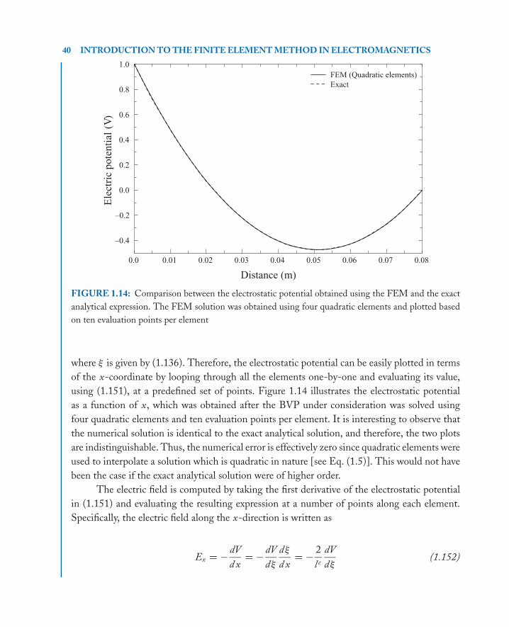
P1: IML/FFX P2: IML/FFX QC: IML/FFX T1: IML
MOBK021-01 MOBK021-Polycarpou.cls April 29, 2006 19:14
40 INTRODUCTION TO THE FINITE ELEMENT METHOD IN ELECTROMAGNETICS
0.0 0.01 0.02 0.03 0.04 0.05 0.06 0.07 0.08
Distance (m)
–0.4
–0.2
0.0
0.2
0.4
0.6
0.8
1.0
Ele
ctri
cpote
nti
al(V
)
FEM (Quadratic elements)
Exact
FIGURE 1.14: Comparison between the electrostatic potential obtained using the FEM and the exact
analytical expression. The FEM solution was obtained using four quadratic elements and plotted based
on ten evaluation points per element
where ξ is given by (1.136). Therefore, the electrostatic potential can be easily plotted in terms
of the x-coordinate by looping through all the elements one-by-one and evaluating its value,
using (1.151), at a predefined set of points. Figure 1.14 illustrates the electrostatic potential
as a function of x, which was obtained after the BVP under consideration was solved using
four quadratic elements and ten evaluation points per element. It is interesting to observe that
the numerical solution is identical to the exact analytical solution, and therefore, the two plots
are indistinguishable. Thus, the numerical error is effectively zero since quadratic elements were
used to interpolate a solution which is quadratic in nature [see Eq. (1.5)]. This would not have
been the case if the exact analytical solution were of higher order.
The electric field is computed by taking the first derivative of the electrostatic potential
in (1.151) and evaluating the resulting expression at a number of points along each element.
Specifically, the electric field along the x-direction is written as
Ex = −dV
d x= −dV
dξ
dξ
d x= − 2
l e
dV
dξ(1.152)

P1: IML/FFX P2: IML/FFX QC: IML/FFX T1: IML
MOBK021-01 MOBK021-Polycarpou.cls April 29, 2006 19:14
ONE-DIMENSIONAL BOUNDARY-VALUE PROBLEMS 41
Substituting (1.151) into (1.152), the x-directed electric field in the region between the two
parallel plates using quadratic shape functions can be expressed as
Ex = − 2
l e
[V e
1
(ξ − 1
2
)+ V e
2
(ξ + 1
2
)+ V e
3 (−2ξ )
](1.153)
where ξ is given by (1.136). To evaluate the electric field in the domain, we must loop through
all the elements and, for each element, evaluate the expression (1.153) at a selected number of
points. Using ten evaluation points per element, the x-directed electric field between the two
parallel plates is shown plotted in Figure 1.15. As was the case with the electrostatic potential,
the finite element solution is identical to the exact analytical solution, thus resulting in zero
numerical error. The reason stems from the fact that the exact expression of the electric field
within the two parallel plates is linear in nature [see Eq. (1.7)] and, as a result, quadratic shape
functions can adequately represent linear variation of a quantity that is proportional to the first
derivative of the primary unknown quantity. It is worth emphasizing here that the numerical
error is not identical to zero but close to the machine error of the computer used to perform the
computations.
0.0 0.01 0.02 0.03 0.04 0.05 0.06 0.07 0.08
Distance (m)
–40
–30
–20
–10
0
10
20
30
40
50
60
Ele
ctri
cfi
eld
(V/m
)
FEM (Quadratic elements)
Exact
FIGURE 1.15: Comparison between the electric field obtained using the FEM and the exact analytical
expression. The FEM solution was obtained using four quadratic elements and plotted based on ten
evaluation points per element
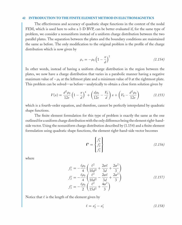
P1: IML/FFX P2: IML/FFX QC: IML/FFX T1: IML
MOBK021-01 MOBK021-Polycarpou.cls April 29, 2006 19:14
42 INTRODUCTION TO THE FINITE ELEMENT METHOD IN ELECTROMAGNETICS
The effectiveness and accuracy of quadratic shape functions in the context of the nodal
FEM, which is used here to solve a 1-D BVP, can be better evaluated if, for the same type of
problem, we consider a nonuniform instead of a uniform charge distribution between the two
parallel plates. The separation between the plates and the boundary conditions are maintained
the same as before. The only modification to the original problem is the profile of the charge
distribution which is now given by
ρv = −ρ0
(1 − x
d
)2
(1.154)
In other words, instead of having a uniform charge distribution in the region between the
plates, we now have a charge distribution that varies in a parabolic manner having a negative
maximum value of −ρ0 at the leftmost plate and a minimum value of 0 at the rightmost plate.
This problem can be solved—as before—analytically to obtain a close form solution given by
V (x) = d 2ρ0
12ε
(1 − x
d
)4
+(
dρ0
12ε− V0
d
)x +
(V0 − d 2ρ0
12ε
)(1.155)
which is a fourth-order equation, and therefore, cannot be perfectly interpolated by quadratic
shape functions.
The finite element formulation for this type of problem is exactly the same as the one
outlined for a uniform charge distribution with the only difference being the element right-hand-
side vector. Using the nonuniform charge distribution described by (1.154) and a finite element
formulation using quadratic shape functions, the element right-hand-side vector becomes
f e =
⎧⎪⎨⎪⎩f e1
f e2
f e3
⎫⎪⎬⎪⎭ (1.156)
where
f e1 = −�ρ0
4
(�2
10d 2+ 2α�
3d+ 2α2
3
)f e2 = −�ρ0
4
(�2
10d 2− 2α�
3d+ 2α2
3
)f e3 = −�ρ0
2
(�2
15d 2+ 4α2
3
) (1.157)
Notice that � is the length of the element given by
� = xe2 − xe
1 (1.158)

P1: IML/FFX P2: IML/FFX QC: IML/FFX T1: IML
MOBK021-01 MOBK021-Polycarpou.cls April 29, 2006 19:14
ONE-DIMENSIONAL BOUNDARY-VALUE PROBLEMS 43
and
α = 1 − xe3
d(1.159)
Using this formulation of the right-hand-side vector, the BVP at hand was solved for a
nonuniform charge distribution using quadratic shape functions. The distribution of the gov-
erning electrostatic potential is plotted in Figures 1.16(a) and 1.16(b) using a two-element mesh
and a four-element mesh, respectively. In both figures, the exact analytical solution, given by
(1.155), is provided for the purpose of comparison. It can be clearly seen that the numerical
solution closely approaches the exact solution as the number of quadratic elements in the mesh
is increased. The same conclusive remark applies to the electric field. However, the electric
field is linearly interpolated because it is computed from the gradient of the electrostatic po-
tential. In addition, there is a discontinuity of the electric field at element boundaries. This was
the case with linear elements as well. This discontinuity of the secondary unknown quantity
tends to become increasingly smaller as the number of elements increases. Note that the un-
derlined weak formulation and associated shape functions guarantee continuity of the primary
unknown quantity across elements but not necessarily of the secondary unknown quantity. This
is demonstrated by plotting the electric field distribution between the two parallel plates for
a two-element mesh and a four-element mesh using quadratic shape functions. The corre-
sponding graphs, together with the exact analytical solution, are illustrated in Figures 1.17(a)
and 1.17(b), respectively. Once again, the finite element solution, for both the electrostatic
potential and the electric field, becomes more accurate as the number of quadratic elements
increases.
The accuracy of the numerical solution can be evaluated by computing the numerical
error, based either on the area bounded between the two curves or the definition of L2 norm,
as a function of the number of quadratic elements. This was done here using the first definition
of numerical error, i.e., based on the area bounded between the finite element solution and
the exact analytical solution. This is referred to as the numerical percent error. A plot of the
numerical percent error, as far as the computation of the electrostatic potential is concerned, as a
function of the number of quadratic elements is depicted in Figure 1.18. Comparing this graph
with the corresponding graph of Figure 1.8(a), which depicts the percent error between the two
solutions but using linear instead of quadratic functions, it is clear that the rate of convergence
has increased significantly with the use of quadratic shape functions. Specifically, with the use
of 20 quadratic elements, the percent error has dropped down to 10−3, whereas in the case of
using 20 linear shape functions the percent error is close to 1. The rate of convergence using
quadratic shape functions can be more clearly seen from Table 1.3, which tabulates the data
that corresponds to the graph illustrated in Figure 1.18. From this table, one can deduce that
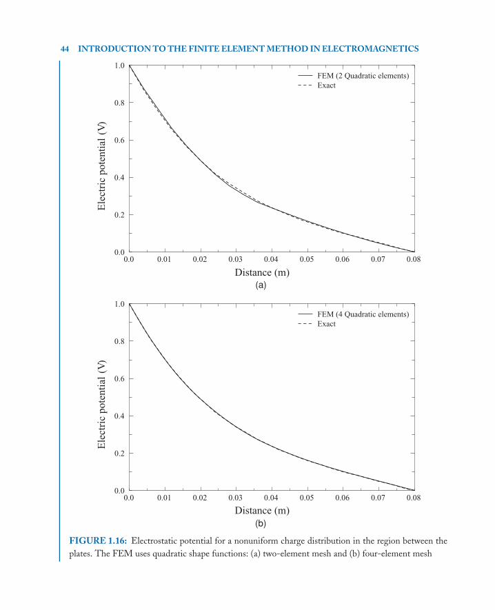
P1: IML/FFX P2: IML/FFX QC: IML/FFX T1: IML
MOBK021-01 MOBK021-Polycarpou.cls April 29, 2006 19:14
44 INTRODUCTION TO THE FINITE ELEMENT METHOD IN ELECTROMAGNETICS
0.0 0.01 0.02 0.03 0.04 0.05 0.06 0.07 0.08
Distance (m)
0.0
0.2
0.4
0.6
0.8
1.0
Ele
ctri
cpote
nti
al(V
)
FEM (2 Quadratic elements)
Exact
(a)
0.0 0.01 0.02 0.03 0.04 0.05 0.06 0.07 0.08
Distance (m)
0.0
0.2
0.4
0.6
0.8
1.0
Ele
ctri
cpote
nti
al(V
)
FEM (4 Quadratic elements)
Exact
(b)
FIGURE 1.16: Electrostatic potential for a nonuniform charge distribution in the region between the
plates. The FEM uses quadratic shape functions: (a) two-element mesh and (b) four-element mesh
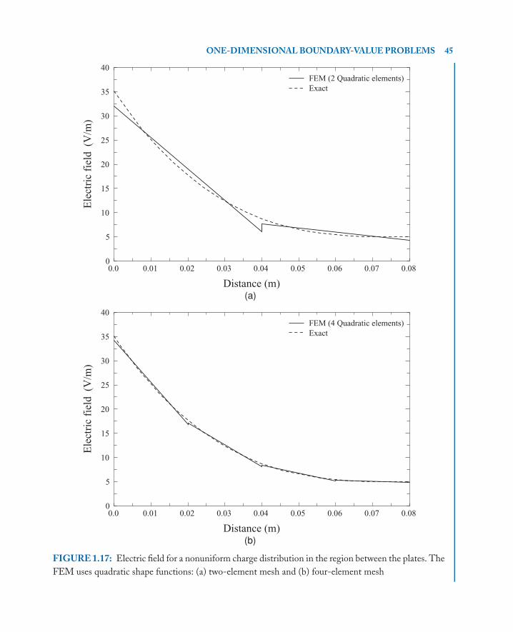
P1: IML/FFX P2: IML/FFX QC: IML/FFX T1: IML
MOBK021-01 MOBK021-Polycarpou.cls April 29, 2006 19:14
ONE-DIMENSIONAL BOUNDARY-VALUE PROBLEMS 45
0.0 0.01 0.02 0.03 0.04 0.05 0.06 0.07 0.08
Distance (m)
0
5
10
15
20
25
30
35
40
Ele
ctri
cfi
eld
(V/m
)FEM (2 Quadratic elements)
Exact
(a)
0.0 0.01 0.02 0.03 0.04 0.05 0.06 0.07 0.08
Distance (m)
0
5
10
15
20
25
30
35
40
Ele
ctri
cfi
eld
(V/m
)
FEM (4 Quadratic elements)
Exact
(b)
FIGURE 1.17: Electric field for a nonuniform charge distribution in the region between the plates. The
FEM uses quadratic shape functions: (a) two-element mesh and (b) four-element mesh
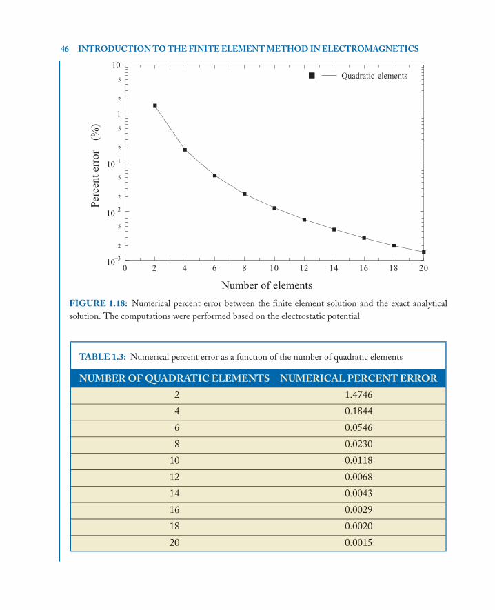
P1: IML/FFX P2: IML/FFX QC: IML/FFX T1: IML
MOBK021-01 MOBK021-Polycarpou.cls April 29, 2006 19:14
46 INTRODUCTION TO THE FINITE ELEMENT METHOD IN ELECTROMAGNETICS
0 2 4 6 8 10 12 14 16 18 2
Number of elements
010
–3
2
5
10–2
2
5
10–1
2
5
1
2
5
10
Per
cent
erro
r(%
)
Quadratic elements
FIGURE 1.18: Numerical percent error between the finite element solution and the exact analytical
solution. The computations were performed based on the electrostatic potential
TABLE 1.3: Numerical percent error as a function of the number of quadratic elements
NUMBER OF QUADRATIC ELEMENTS NUMERICAL PERCENT ERROR
2 1.4746
4 0.1844
6 0.0546
8 0.0230
10 0.0118
12 0.0068
14 0.0043
16 0.0029
18 0.0020
20 0.0015

P1: IML/FFX P2: IML/FFX QC: IML/FFX T1: IML
MOBK021-01 MOBK021-Polycarpou.cls April 29, 2006 19:14
ONE-DIMENSIONAL BOUNDARY-VALUE PROBLEMS 47
the percent error drops by a factor of 8 if the number of quadratic elements is doubled, whereas
in the case of linear shape functions, this factor was 4.
Exercise1.6. Show that (1.155) is indeed the analytical solution of the BVP at hand. Remember
that the electron charge distribution in the region between the two parallel plates has changed
from a constant profile to a parabolic profile given by (1.154).
Exercise 1.7. Using quadratic elements and the formulation presented in Section 1.11 for the
derivation of the element right-hand-side vector f e, show that the latter is given by (1.156)–
(1.159).
1.14 POSTPROCESSING OF THE SOLUTION: CUBIC ELEMENTSThe major steps involved in the postprocessing of the finite element solution obtained using cubic
elements are identical to the steps involved in the postprocessing of the finite element solution
obtained using quadratic elements. The only difference is the order of shape functions used to
interpolate the primary unknown variable over an element. To avoid unnecessary repetitions, we
will restrict our discussion on the development of the governing expansion equations describing
the primary and secondary unknown variables over an element after the finite element solution
has been obtained. It will be left as an exercise for the reader to repeat, using cubic elements,
the same procedure as was done in the previous section, using quadratic elements, for the
computation of the numerical percent error between the exact and the finite element solutions
and to compare the result with Figure 1.18 or Table 1.3.
Solving the global matrix system after imposing the governing Dirichlet boundary condi-
tions, a set of values for the primary unknown variable (i.e., electrostatic potential) is obtained.
These values correspond to the global nodes of the finite element mesh. For someone to plot
the primary unknown variable with good enough resolution in the discretized domain, it is nec-
essary that the primary unknown variable be evaluated at multiple points along each element.
When using cubic shape functions, the electrostatic potential is given by
V = V e1 N1(x) + V e
2 N2(x) + V e3 N3(x) + V e
4 N4(x) (1.160)
where V ei for i = 1, 2, 3, 4 are the values of the electrostatic potential at the four nodes of the
element, and Ni (x) for i = 1, 2, 3, 4 are the corresponding cubic shape functions in terms of x.
The cubic shape functions expressed in terms of x are obtained by substituting (1.132) into the
set of four equations given by (1.129) and (1.130).
As was done with quadratic elements, the electric field over a cubic element is computed
by taking the first derivative of (1.160) and evaluating the resulting expression at a selection of
points along the element. This derivative can be evaluated more conveniently by implementing
P1: IML/FFX P2: IML/FFX QC: IML/FFX T1: IML
MOBK021-01 MOBK021-Polycarpou.cls April 29, 2006 19:14
48 INTRODUCTION TO THE FINITE ELEMENT METHOD IN ELECTROMAGNETICS
the chain rule of differentiation
Ex = −dV
d x= −dV
dξ
dξ
d x= − 2
l e
dV
dξ= − 2
l e
4∑i=1
V ei
(dNi
dξ
)(1.161)
where Ni for i = 1, 2, 3, 4 are given by (1.129) and (1.130). From this discussion, it becomes
clear now that the electric field, which is the secondary unknown variable, is quadratic over a
cubic element whereas the electrostatic potential, which is the primary unknown variable, is
cubic.
1.15 SOFTWAREThree Matlab codes were written in order to solve the electrostatic BVP discussed in this chapter.
The first code, FEM1DL, uses linear elements to solve the Poisson’s equation in one dimension
assuming that the charge distribution between the two parallel plates is uniform. Dirichlet
boundary conditions are imposed on the two plates. The code computes both the electrostatic
potential and the electric field within the domain of interest. The second code, FEM1DQ,
uses quadratic elements to solve the same exact problem. The third code, FEM1Dqnucd, uses
quadratic elements to solve the same problem but with a nonuniform, instead of uniform, charge
distribution. All three codes are capable of computing the numerical error associated with the
finite element solution. Certain parameters such as mesh size and separation of plates can be
modified by the user. All three Matlab codes can be downloaded from the publisher’s URL:
www.morganclaypool.com/page/polycarpou.
Exercise 1.8. Write a finite element code in Matlab to solve the same BVP considered in
this chapter but using cubic elements instead of linear or quadratic elements. Assume that
the electron charge distribution between the plates is given by (1.154). Compute and plot the
numerical error, either as a percentage or using the L2-norm definition, and compare with
Tables 1.2 and 1.3.
REFERENCES[1] O. C. Zienkiewicz, The Finite Element Method. New York: McGraw-Hill, 1977.
[2] P. P. Silvester and R. L. Ferrari, Finite Elements for Electrical Engineers, 2nd ed. London:
Cambridge University Press, 1990.
[3] J. Jin, The Finite Element Method in Electromagnetics, 2nd ed. New York: Wiley-IEEE
Press, 2002.
[4] J. L. Volakis, A. Chatterjee, and L. C. Kempel, Finite Element Method Electromagnetics:
Antennas, Microwave Circuits, and Scattering Applications. New York: Wiley-IEEE Press,
1998.
P1: IML/FFX P2: IML/FFX QC: IML/FFX T1: IML
MOBK021-01 MOBK021-Polycarpou.cls April 29, 2006 19:14
ONE-DIMENSIONAL BOUNDARY VALUE PROBLEMS 49
[5] G. Pelosi, R. Coccioli, and S. Selleri, Quick Finite Elements For Electromagnetic Waves.
Boston: Artech House, 1998.
[6] J. N. Reddy, Applied Functional Analysis and Variational Methods in Engineering. New
York: McGraw-Hill, 1986.
[7] S. G. Mikhlin, Variational Methods in Mathematical Physics. New York: Macmillan, 1964.
[8] M. N. O. Sadiku, Numerical Techniques in Electromagnetics, 2nd ed. Boca Raton: CRC
Press, 2001.
[9] D. K. Cheng, Fundamentals of Engineering Electromagnetics. New York: Addison-Wesley,
1993.
[10] C. H. Edwards, Jr., and D. E. Penney, Elementary Linear Algebra. New Jersey: Prentice-
Hall, 1988.

P1: IML/FFX P2: IML/FFX QC: IML/FFX T1: IML
MOBK021-01 MOBK021-Polycarpou.cls April 29, 2006 19:14
50
P1: IML/FFX P2: IML
MOBK021-02 MOBK021-Polycarpou.cls April 29, 2006 20:28
51
C H A P T E R 2
Two-Dimensional
Boundary-Value Problems
2.1 INTRODUCTIONIn this chapter, the nodal FEM will be applied to a generic 2-D BVP in electromagnetics. Such
problems usually involve a second-order differential equation of a single dependent variable that
is subject to a set of boundary conditions. These boundary conditions could be of the Dirichlet
type, the Neumann type, or the mixed type. The domain of the problem is a 2-D geometry
with an arbitrary shape. Thus, an accurate representation of the domain in the context of the
FEM presumes discretization of the domain using the most appropriate shape of basic elements
called the finite elements. The most commonly used finite elements in two dimensions are the
triangular and quadrilateral elements. Both types of elements will be used in this chapter to solve
2-D BVPs in electromagnetics. Furthermore, higher order elements will be used to illustrate the
improvement in accuracy of the numerical solution without necessarily increasing the number
of elements in the finite element mesh.
The major steps involved in the application of the FEM for the solution of 2-D BVPs are
identical to those involved in the solution of 1-D problems. Specifically, a proper application
of the FEM for the solution of 2-D BVPs must involve the following major steps:
a) Discretization of the 2-D domain.
b) Derivation of the weak formulation of the governing differential equation.
c) Proper choice of interpolation functions.
d) Derivation of the element matrices and vectors.
e) Assembly of the global matrix system.
f ) Imposition of boundary conditions.
g) Solution of the global matrix system.
h) Postprocessing of the results.
Problem definition: A BVP characterized by a generic form of a second-order partial differential
equation will be considered in this chapter to illustrate the major steps involved in a 2-D nodal

P1: IML/FFX P2: IML
MOBK021-02 MOBK021-Polycarpou.cls April 29, 2006 20:28
52 INTRODUCTION TO THE FINITE ELEMENT METHOD IN ELECTROMAGNETICS
FEM. This generic type partial differential equation can be expressed as
∂
∂x
(αx
∂u
∂x
)+ ∂
∂y
(αy
∂u
∂y
)+ βu = g (2.1)
where αx , αy , β, and g are constants to be defined by the specific application and u is the primary
unknown quantity. Poisson’s equation, for a linear and isotropic medium, is given by
∇ (ε∇V ) = −ρv (2.2)
In a 2-D space, (2.2) is often written as
∂
∂x
(ε∂V
∂x
)+ ∂
∂y
(ε∂V
∂y
)= −ρv (2.3)
Equation (2.3) is a special case of the generic form given by (2.1). Comparing (2.1) with (2.3),
it can be easily realized that these two partial differential equations would be identical if
u = V
αx = αy = ε (2.4)
β = 0
g = −ρv
Consequently, the 2-D Poisson’s equation, which is widely used to solve electrostatic problems,
is a special case of (2.1). The set of boundary conditions could be either of Dirichlet type
u = u0 on �1 (2.5)
or mixed type (αx
∂u
∂xax + αy
∂u
∂ya y
)· an + γ u = q on �2 (2.6)
where an is the unit vector normal to the boundary �2 and γ, q are constants to be defined.
2.2 DOMAIN DISCRETIZATIONThe domain of a 2-D BVP usually has an irregular shape, as shown in Figure 2.1(a). Using
the FEM, the first step is to accurately represent the physical domain of the problem by a set
of basic shapes called the finite elements. The use of a rectangle, for example, as a basic finite
element to discretize an irregular domain is certainly the simplest but not the most suitable
choice because an assembly of rectangles cannot accurately represent the arbitrary geometrical
shape of the domain. In such a case, the discretization error is significant, as shown in Figure
2.1(b), although it tends to decrease as the size of rectangles in the domain becomes smaller. On
the other hand, if a triangle is used instead of a rectangle as the basic element for the meshing of
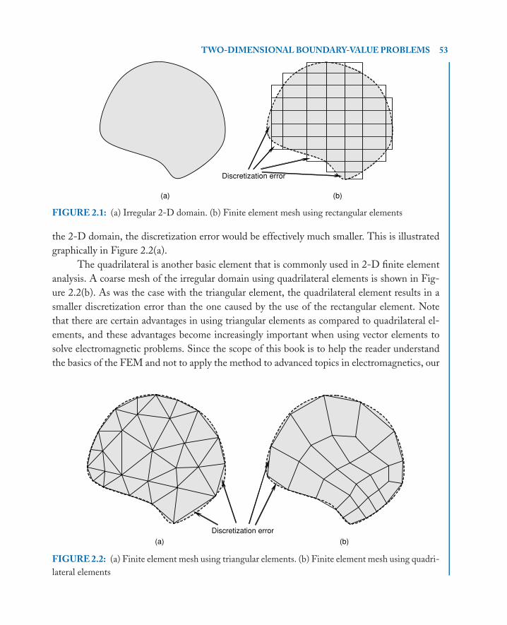
P1: IML/FFX P2: IML
MOBK021-02 MOBK021-Polycarpou.cls April 29, 2006 20:28
TWO-DIMENSIONAL BOUNDARY-VALUE PROBLEMS 53
Discretization error
(a) (b)
FIGURE 2.1: (a) Irregular 2-D domain. (b) Finite element mesh using rectangular elements
the 2-D domain, the discretization error would be effectively much smaller. This is illustrated
graphically in Figure 2.2(a).
The quadrilateral is another basic element that is commonly used in 2-D finite element
analysis. A coarse mesh of the irregular domain using quadrilateral elements is shown in Fig-
ure 2.2(b). As was the case with the triangular element, the quadrilateral element results in a
smaller discretization error than the one caused by the use of the rectangular element. Note
that there are certain advantages in using triangular elements as compared to quadrilateral el-
ements, and these advantages become increasingly important when using vector elements to
solve electromagnetic problems. Since the scope of this book is to help the reader understand
the basics of the FEM and not to apply the method to advanced topics in electromagnetics, our
Discretization error
(a) (b)
FIGURE 2.2: (a) Finite element mesh using triangular elements. (b) Finite element mesh using quadri-
lateral elements
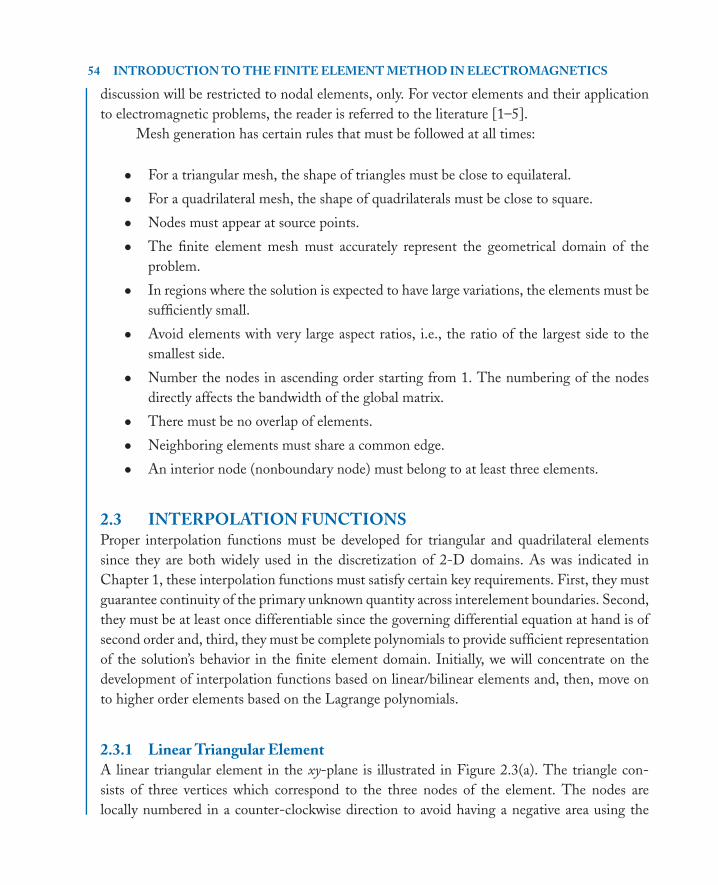
P1: IML/FFX P2: IML
MOBK021-02 MOBK021-Polycarpou.cls April 29, 2006 20:28
54 INTRODUCTION TO THE FINITE ELEMENT METHOD IN ELECTROMAGNETICS
discussion will be restricted to nodal elements, only. For vector elements and their application
to electromagnetic problems, the reader is referred to the literature [1–5].
Mesh generation has certain rules that must be followed at all times:
• For a triangular mesh, the shape of triangles must be close to equilateral.
• For a quadrilateral mesh, the shape of quadrilaterals must be close to square.
• Nodes must appear at source points.
• The finite element mesh must accurately represent the geometrical domain of the
problem.
• In regions where the solution is expected to have large variations, the elements must be
sufficiently small.
• Avoid elements with very large aspect ratios, i.e., the ratio of the largest side to the
smallest side.
• Number the nodes in ascending order starting from 1. The numbering of the nodes
directly affects the bandwidth of the global matrix.
• There must be no overlap of elements.
• Neighboring elements must share a common edge.
• An interior node (nonboundary node) must belong to at least three elements.
2.3 INTERPOLATION FUNCTIONSProper interpolation functions must be developed for triangular and quadrilateral elements
since they are both widely used in the discretization of 2-D domains. As was indicated in
Chapter 1, these interpolation functions must satisfy certain key requirements. First, they must
guarantee continuity of the primary unknown quantity across interelement boundaries. Second,
they must be at least once differentiable since the governing differential equation at hand is of
second order and, third, they must be complete polynomials to provide sufficient representation
of the solution’s behavior in the finite element domain. Initially, we will concentrate on the
development of interpolation functions based on linear/bilinear elements and, then, move on
to higher order elements based on the Lagrange polynomials.
2.3.1 Linear Triangular Element
A linear triangular element in the xy-plane is illustrated in Figure 2.3(a). The triangle con-
sists of three vertices which correspond to the three nodes of the element. The nodes are
locally numbered in a counter-clockwise direction to avoid having a negative area using the
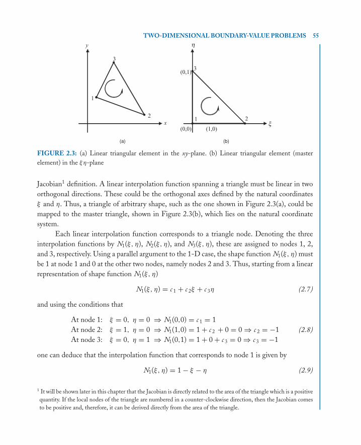
P1: IML/FFX P2: IML
MOBK021-02 MOBK021-Polycarpou.cls April 29, 2006 20:28
TWO-DIMENSIONAL BOUNDARY-VALUE PROBLEMS 55
x
y
1
2
3
1 2
3
(a) (b)
(0,0) (1,0)
(0,1)
x
h
FIGURE 2.3: (a) Linear triangular element in the xy-plane. (b) Linear triangular element (master
element) in the ξη-plane
Jacobian1 definition. A linear interpolation function spanning a triangle must be linear in two
orthogonal directions. These could be the orthogonal axes defined by the natural coordinates
ξ and η. Thus, a triangle of arbitrary shape, such as the one shown in Figure 2.3(a), could be
mapped to the master triangle, shown in Figure 2.3(b), which lies on the natural coordinate
system.
Each linear interpolation function corresponds to a triangle node. Denoting the three
interpolation functions by N1(ξ, η), N2(ξ, η), and N3(ξ, η), these are assigned to nodes 1, 2,
and 3, respectively. Using a parallel argument to the 1-D case, the shape function N1(ξ, η) must
be 1 at node 1 and 0 at the other two nodes, namely nodes 2 and 3. Thus, starting from a linear
representation of shape function N1(ξ, η)
N1(ξ, η) = c 1 + c 2ξ + c 3η (2.7)
and using the conditions that
At node 1: ξ = 0, η = 0 ⇒ N1(0,0) = c 1 = 1
At node 2: ξ = 1, η = 0 ⇒ N1(1,0) = 1 + c 2 + 0 = 0 ⇒ c 2 = −1 (2.8)
At node 3: ξ = 0, η = 1 ⇒ N1(0,1) = 1 + 0 + c 3 = 0 ⇒ c 3 = −1
one can deduce that the interpolation function that corresponds to node 1 is given by
N1(ξ, η) = 1 − ξ − η (2.9)
1 It will be shown later in this chapter that the Jacobian is directly related to the area of the triangle which is a positive
quantity. If the local nodes of the triangle are numbered in a counter-clockwise direction, then the Jacobian comes
to be positive and, therefore, it can be derived directly from the area of the triangle.
P1: IML/FFX P2: IML
MOBK021-02 MOBK021-Polycarpou.cls April 29, 2006 20:28
56 INTRODUCTION TO THE FINITE ELEMENT METHOD IN ELECTROMAGNETICS
Similarly, N2(ξ, η) must be 1 at node 2 and 0 at nodes 1 and 3. A linear representation of
N2(ξ, η) is
N2(ξ,η) = c 1 + c 2ξ + c 3η (2.10)
Imposing the above conditions, we have
At node 1: ξ = 0, η = 0 ⇒ N2(0,0) = c 1 = 0
At node 2: ξ = 1, η = 0 ⇒ N2(1,0) = 0 + c 2 + 0 = 1 ⇒ c 2 = 1 (2.11)
At node 3: ξ = 0, η = 1 ⇒ N2(0,1) = 0 + 0 + c 3 = 0 ⇒ c 3 = 0
Thus,
N2(ξ,η) = ξ (2.12)
Finally, N3(ξ, η) must be 1 at node 3 and 0 at the other two nodes of the master triangle. In
general, N3(ξ, η) can be expressed as
N3(ξ, η) = c 1 + c 2ξ + c 3η (2.13)
To obtain constants c 1, c 2, and c 3, the above conditions must be imposed, i.e.,
At node 1: ξ = 0, η = 0 ⇒ N3(0, 0) = c 1 = 0
At node 2: ξ = 1, η = 0 ⇒ N3(1, 0) = c 2 = 0 (2.14)
At node 3: ξ = 0, η = 1 ⇒ N3(0, 1) = c 3 = 1
The final form of N3(ξ, η) is therefore given by
N3(ξ, η) = η (2.15)
These three interpolation functions are plotted in Figure 2.4. It is important to empha-
size here that these interpolation functions are not linearly independent. Only N2 and N3 are
independent; N1 is a linear combination of N2 and N3; i.e.,
N1 = 1 − N2 − N3 (2.16)
which can also be written as
N1 + N2 + N3 = 1 (2.17)
These triangle-based linear interpolation functions can also be written in terms of area
coordinates. Consider an arbitrary point (ξ , η) inside the master triangle shown in Figure 2.5.
Connecting all three vertices to the interior point (ξ , η), three subtriangles are formed with
respective areas A1, A2, and A3. Note that A1 corresponds to the subtriangle opposite to local

P1: IML/FFX P2: IML
MOBK021-02 MOBK021-Polycarpou.cls April 29, 2006 20:28
TWO-DIMENSIONAL BOUNDARY-VALUE PROBLEMS 57
2
3
1
1
N2
1
3
2
1
2
3N3
1
1
N1
xx
h
h
h
x
FIGURE 2.4: Linear triangular interpolation functions
, )
2
3
2
3
A1
A
x
(
1
A
x h
h
FIGURE 2.5: Area coordinates
P1: IML/FFX P2: IML
MOBK021-02 MOBK021-Polycarpou.cls April 29, 2006 20:28
58 INTRODUCTION TO THE FINITE ELEMENT METHOD IN ELECTROMAGNETICS
node 1. A similar notation applies to the other two subtriangles. Based on this notation, the
linear interpolation functions N1, N2, and N3 can be expressed as
N1 = A1
A
N2 = A2
A(2.18)
N3 = A3
A
where A is the area of the master triangle. Notice that
N1 + N2 + N3 = A1
A+ A2
A+ A3
A
= A1 + A2 + A3
A(2.19)
= A
A= 1
This set of triangular basis functions are used in the FEM to interpolate the primary
unknown quantity in the interior of an element. In case of using linear triangular elements to
discretize the problem domain, the primary unknown quantity—let us say u—inside an element
can be expressed as
u = ue1 N1 + ue
2 N2 + ue3 N3 =
3∑i=1
uei Ni (2.20)
where ue1, ue
2, and ue3 are the nodal values of the primary unknown quantity at the three vertices
of the triangle. For isoparametric elements, the same shape functions used to interpolate the
primary unknown quantity inside an element are also used to interpolate the space coordinates
x and y . In other words,
x = xe1 N1 + xe
2 N2 + xe3 N3 =
3∑i=1
xei Ni
y = ye1 N1 + ye
2 N2 + ye3 N3 =
3∑i=1
yei Ni (2.21)
Substituting N1, N2, and N3 into (2.21) yields
x = xe1 + x21ξ + x31η
y = ye1 + y21ξ + y31η (2.22)
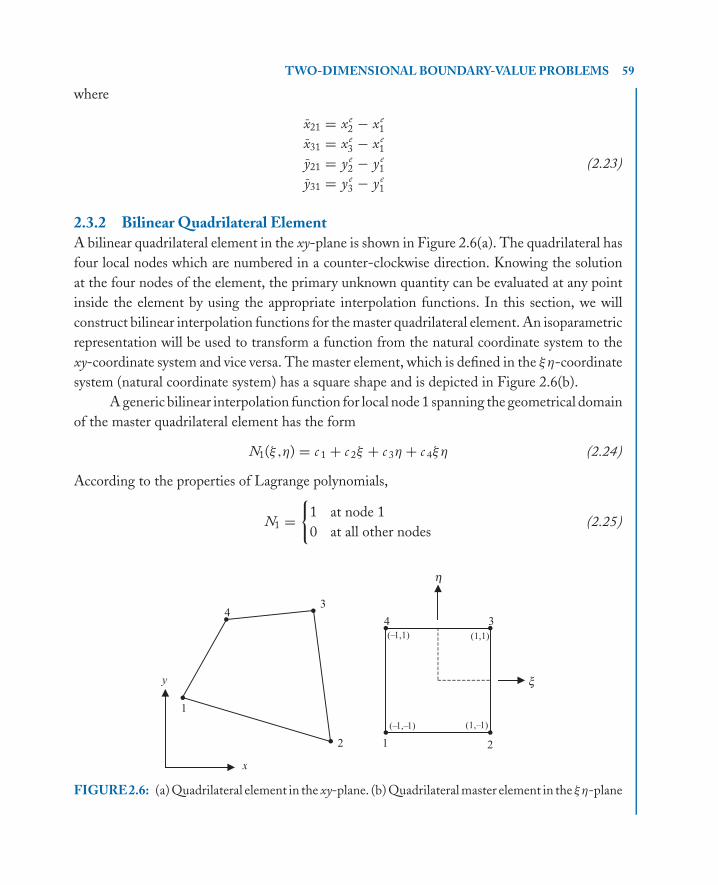
P1: IML/FFX P2: IML
MOBK021-02 MOBK021-Polycarpou.cls April 29, 2006 20:28
TWO-DIMENSIONAL BOUNDARY-VALUE PROBLEMS 59
where
x21 = xe2 − xe
1
x31 = xe3 − xe
1
y21 = ye2 − ye
1 (2.23)
y31 = ye3 − ye
1
2.3.2 Bilinear Quadrilateral Element
A bilinear quadrilateral element in the xy-plane is shown in Figure 2.6(a). The quadrilateral has
four local nodes which are numbered in a counter-clockwise direction. Knowing the solution
at the four nodes of the element, the primary unknown quantity can be evaluated at any point
inside the element by using the appropriate interpolation functions. In this section, we will
construct bilinear interpolation functions for the master quadrilateral element. An isoparametric
representation will be used to transform a function from the natural coordinate system to the
xy-coordinate system and vice versa. The master element, which is defined in the ξη-coordinate
system (natural coordinate system) has a square shape and is depicted in Figure 2.6(b).
A generic bilinear interpolation function for local node 1 spanning the geometrical domain
of the master quadrilateral element has the form
N1(ξ,η) = c 1 + c 2ξ + c 3η + c 4ξη (2.24)
According to the properties of Lagrange polynomials,
N1 ={
1 at node 1
0 at all other nodes(2.25)
x
y
4
1
(–1,1) (1,1)
3
(1,–1)
1
3 4
2
(–1,–1)
2
x
h
FIGURE2.6: (a) Quadrilateral element in the xy-plane. (b) Quadrilateral master element in the ξη-plane
P1: IML/FFX P2: IML
MOBK021-02 MOBK021-Polycarpou.cls April 29, 2006 20:28
60 INTRODUCTION TO THE FINITE ELEMENT METHOD IN ELECTROMAGNETICS
Applying these conditions at the four nodes of the master quadrilateral element, the result is a
system of four equations with four unknowns, the unknowns being the four constants of (2.24).
N1(−1,−1) = c 1 − c 2 − c 3 + c 4 = 1
N1(1,−1) = c 1 + c 2 − c 3 − c 4 = 0
N1(1,1) = c 1 + c 2 + c 3 + c 4 = 0 (2.26)
N1(−1,1) = c 1 − c 2 + c 3 − c 4 = 0
This system of equations can be solved in a straightforward manner to obtain the constants. It
can be shown that
c 1 = 14, c 2 = − 1
4, c 3 = − 1
4, c 4 = 1
4(2.27)
Thus, the interpolation function that corresponds to node 1 is given by
N1(ξ,η) = 14(1 − ξ − η + ξη) (2.28)
which can also be written as
N1(ξ,η) = 14(1 − ξ )(1 − η) (2.29)
Using a similar approach, one can construct all four bilinear interpolation functions spanning a
quadrilateral element:
N1(ξ,η) = 14(1 − ξ )(1 − η)
N2(ξ,η) = 14(1 + ξ )(1 − η)
N3(ξ,η) = 14(1 + ξ )(1 + η) (2.30)
N4(ξ,η) = 14(1 − ξ )(1 + η)
Assuming an isoparametric quadrilateral element, the primary unknown quantity and
the x and y space coordinates inside an element can be expressed in terms of these four basis
functions given by (2.30). In other words,
u = ue1 N1 + ue
2 N2 + ue3 N3 + ue
4 N4 =4∑
i=1
uei Ni (2.31)
and
x = xe1 N1 + xe
2 N2 + xe3 N3 + xe
4 N4 =4∑
i=1
xei Ni
y = ye1 N1 + ye
2 N2 + ye3 N3 + ye
4 N4 =4∑
i=1
yei Ni (2.32)

P1: IML/FFX P2: IML
MOBK021-02 MOBK021-Polycarpou.cls April 29, 2006 20:28
TWO-DIMENSIONAL BOUNDARY-VALUE PROBLEMS 61
Exercise 2.1. Show that the shape functions governing a bilinear quadrilateral element are
given by (2.30). Use the same approach followed for the derivation of N1(ξ,η).
2.4 THE METHOD OF WEIGHTED RESIDUAL:THE GALERKIN APPROACH
The generic 2-D BVP considered at the beginning of this chapter is characterized by a second-
order partial differential equation given by
∂
∂x
(αx
∂u
∂x
)+ ∂
∂y
(αy
∂u
∂y
)+ βu = g (2.33)
where αx , αy , β, and g are constants. The weak formulation of this problem can be obtained
by first constructing the weighted residual of (2.33) for a single element with domain �e . The
element residual is formed by moving the right-hand side of (2.33) to the left-hand side:
r e = ∂
∂x
(αx
∂u
∂x
)+ ∂
∂y
(αy
∂u
∂y
)+ βu − g (2.34)
This element residual is ideally zero, provided that the numerical solution u to be obtained is
identical to the exact solution. However, this is not the case, and therefore, the element residual
r e is, in general, nonzero. Our objective is to minimize this element residual in a weighted sense.
To achieve this, we must first multiply r e with a weight function w, then integrate the result
over the area of the element, and finally, set the integral to zero.∫∫�e
w
[∂
∂x
(αx
∂u
∂x
)+ ∂
∂y
(αy
∂u
∂y
)+ βu − g
]d xd y = 0 (2.35)
Introducing the identity
∂
∂x
(wαx
∂u
∂x
)= ∂w
∂x
(αx
∂u
∂x
)+ w
∂
∂x
(αx
∂u
∂x
)(2.36)
which can be rearranged as
w∂
∂x
(αx
∂u
∂x
)= ∂
∂x
(wαx
∂u
∂x
)− ∂w
∂x
(αx
∂u
∂x
)= ∂
∂x
(wαx
∂u
∂x
)− αx
∂w
∂x
∂u
∂x(2.37)
and substituting the latter into (2.35) yields∫∫�e
[∂
∂x
(wαx
∂u
∂x
)+ ∂
∂y
(wαy
∂u
∂y
)]d x d y −
∫∫�e
[αx
∂w
∂x
∂u
∂x+ αy
∂w
∂y
∂u
∂y
]d x d y
+∫∫
�e
βw u d x d y =∫∫
�e
w g d x d y (2.38)
P1: IML/FFX P2: IML
MOBK021-02 MOBK021-Polycarpou.cls April 29, 2006 20:28
62 INTRODUCTION TO THE FINITE ELEMENT METHOD IN ELECTROMAGNETICS
Then, we implement the Green’s theorem which states that the area integral of the divergence
of a vector quantity equals to the total outward flux of the vector quantity through the contour
that bounds the area. In equation form,∫∫�e
(∇t · �A
)d A =
∮�e
�A · and� (2.39)
or simply ∫∫�e
(∂Ax
∂x+ ∂Ay
∂y
)d x d y =
∮�e
(ax Ax + a y Ay
)· and� (2.40)
where �A is the vector quantity of interest and an is the outward unit vector that is normal to the
boundary of the element. The contour integral in (2.40) must be evaluated along the periphery
of the element in a counter-clockwise direction. Comparing the first integral of (2.40) with the
first integral of (2.38), it becomes quite clear that
Ax = wαx∂u
∂x(2.41)
and
Ay = wαy∂u
∂y(2.42)
By defining the normal unit vector as
an = axnx + a y ny (2.43)
and applying the Green’s theorem to the first integral of (2.38), the latter becomes∫∫�e
[∂
∂x
(wαx
∂u
∂x
)+ ∂
∂y
(wαy
∂u
∂y
)]dx dy =
∮�e
w
(αx
∂u
∂xnx + αy
∂u
∂yny
)d� (2.44)
Substituting this result into (2.38), the weak form of the differential equation reduces to
−∫∫
�e
[αx
∂w
∂x
∂u
∂x+ αy
∂w
∂y
∂u
∂y
]dx dy +
∫∫�e
βwu d x d y =∫∫
�e
wg dx dy
−∮
�e
w
(αx
∂u
∂xnx + αy
∂u
∂yny
)d� (2.45)
According to the Galerkin approach, the weight function w must belong to the same set
of shape functions that are used to interpolate the primary unknown quantity which, in our case,
is u. In the previous section, it was shown that the primary unknown quantity is interpolated
P1: IML/FFX P2: IML
MOBK021-02 MOBK021-Polycarpou.cls April 29, 2006 20:28
TWO-DIMENSIONAL BOUNDARY-VALUE PROBLEMS 63
using a set of Lagrange polynomials. Thus,
u =n∑
j=1
uej Nj (2.46)
where Nj ’s are the corresponding shape functions based on Lagrange polynomials and n is the
number of local nodes per element. Substituting (2.46) into (2.45), and setting
w = Ni for i = 1, 2, . . . , n (2.47)
the weak form of the governing differential equation is discretized:
−∫∫
�e
⎡⎢⎢⎢⎢⎣αx∂ Ni
∂x
∂
(n∑
j=1
uej Nj
)∂x
+ αy∂ Ni
∂y
∂
(n∑
j=1
uej Nj
)∂y
⎤⎥⎥⎥⎥⎦ d x d y
+∫∫
�e
βNi
(n∑
j=1
uej Nj
)dx dy =
∫∫�e
Ni g dx dy −∮
�e
Ni
(αx
∂u
∂xnx + αy
∂u
∂yny
)d�,
for i = 1, 2, . . . , n
(2.48)
Notice that the primary unknown quantity u in the contour integral of (2.48) has not been
replaced by the set of interpolation functions given by (2.46). This integral will be treated
separately a bit later. Equation (2.48) can also be written in the following form:
−∫∫
�e
[αx
(∂ Ni
∂x
) (n∑
j=1
uej
∂ Nj
∂x
)+ αy
(∂ Ni
∂y
) (n∑
j=1
uej
∂ Nj
∂y
)]dxdy
+∫∫
�e
βNi
(n∑
j=1
uej Nj
)dx dy =
∫∫�e
Ni g dx dy −∮
�e
Ni
(αx
∂u
∂xnx + αy
∂u
∂yny
)d�,
for i = 1, 2, . . . , n
(2.49)
This equation can be conveniently expressed in a matrix form given by⎡⎢⎢⎢⎢⎣M e
11 Me12 · · · Me
1n
Me21 Me
22 · · · Me2n
......
. . ....
Men1 Me
n2 · · · Menn
⎤⎥⎥⎥⎥⎦⎧⎪⎪⎪⎪⎨⎪⎪⎪⎪⎩
u e1
u e2...
u en
⎫⎪⎪⎪⎪⎬⎪⎪⎪⎪⎭ +
⎡⎢⎢⎢⎢⎣T e
11 T e12 · · · T e
1n
T e21 T e
22 · · · T e2n
......
. . ....
T en1 T e
n2 · · · T enn
⎤⎥⎥⎥⎥⎦⎧⎪⎪⎪⎪⎨⎪⎪⎪⎪⎩
u e1
u e2...
u en
⎫⎪⎪⎪⎪⎬⎪⎪⎪⎪⎭ =
⎧⎪⎪⎪⎪⎨⎪⎪⎪⎪⎩f e1
f e2...
f en
⎫⎪⎪⎪⎪⎬⎪⎪⎪⎪⎭ +
⎧⎪⎪⎪⎪⎨⎪⎪⎪⎪⎩p e
1
p e2...
p en
⎫⎪⎪⎪⎪⎬⎪⎪⎪⎪⎭(2.50)
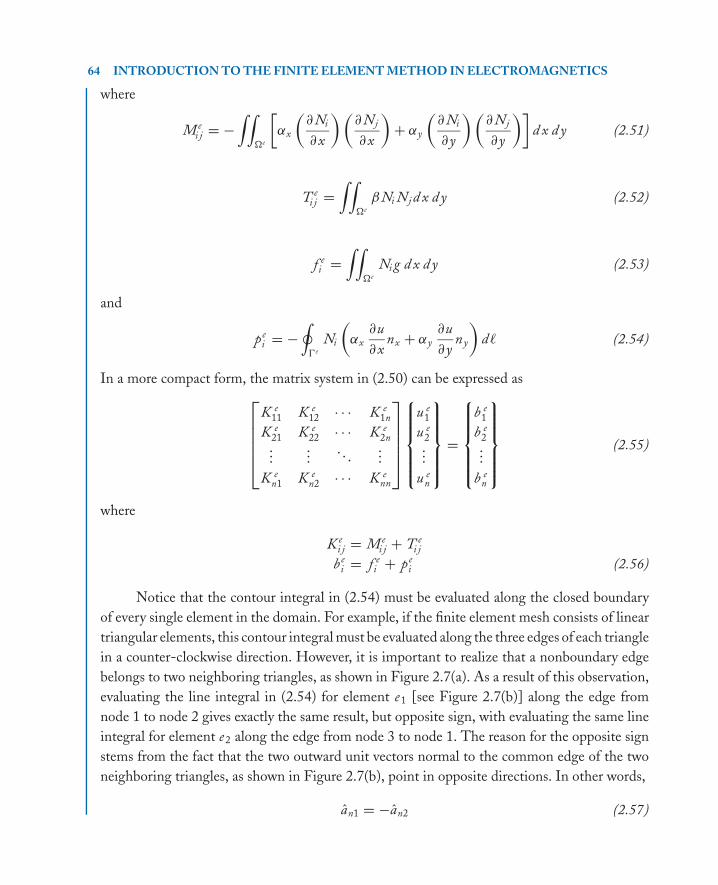
P1: IML/FFX P2: IML
MOBK021-02 MOBK021-Polycarpou.cls April 29, 2006 20:28
64 INTRODUCTION TO THE FINITE ELEMENT METHOD IN ELECTROMAGNETICS
where
Mei j = −
∫∫�e
[αx
(∂ Ni
∂x
) (∂ Nj
∂x
)+ αy
(∂ Ni
∂y
) (∂ Nj
∂y
)]d x d y (2.51)
T ei j =
∫∫�e
βNi Nj d x d y (2.52)
f ei =
∫∫�e
Ni g d x d y (2.53)
and
pei = −
∮�e
Ni
(αx
∂u
∂xnx + αy
∂u
∂yny
)d� (2.54)
In a more compact form, the matrix system in (2.50) can be expressed as⎡⎢⎢⎢⎢⎣K e
11 K e12 · · · K e
1n
K e21 K e
22 · · · K e2n
......
. . ....
K en1 K e
n2 · · · K enn
⎤⎥⎥⎥⎥⎦⎧⎪⎪⎪⎪⎨⎪⎪⎪⎪⎩
u e1
u e2...
u en
⎫⎪⎪⎪⎪⎬⎪⎪⎪⎪⎭ =
⎧⎪⎪⎪⎪⎨⎪⎪⎪⎪⎩b e
1
b e2...
b en
⎫⎪⎪⎪⎪⎬⎪⎪⎪⎪⎭ (2.55)
where
K ei j = Me
i j + T ei j
bei = f e
i + pei (2.56)
Notice that the contour integral in (2.54) must be evaluated along the closed boundary
of every single element in the domain. For example, if the finite element mesh consists of linear
triangular elements, this contour integral must be evaluated along the three edges of each triangle
in a counter-clockwise direction. However, it is important to realize that a nonboundary edge
belongs to two neighboring triangles, as shown in Figure 2.7(a). As a result of this observation,
evaluating the line integral in (2.54) for element e1 [see Figure 2.7(b)] along the edge from
node 1 to node 2 gives exactly the same result, but opposite sign, with evaluating the same line
integral for element e2 along the edge from node 3 to node 1. The reason for the opposite sign
stems from the fact that the two outward unit vectors normal to the common edge of the two
neighboring triangles, as shown in Figure 2.7(b), point in opposite directions. In other words,
an1 = −an2 (2.57)
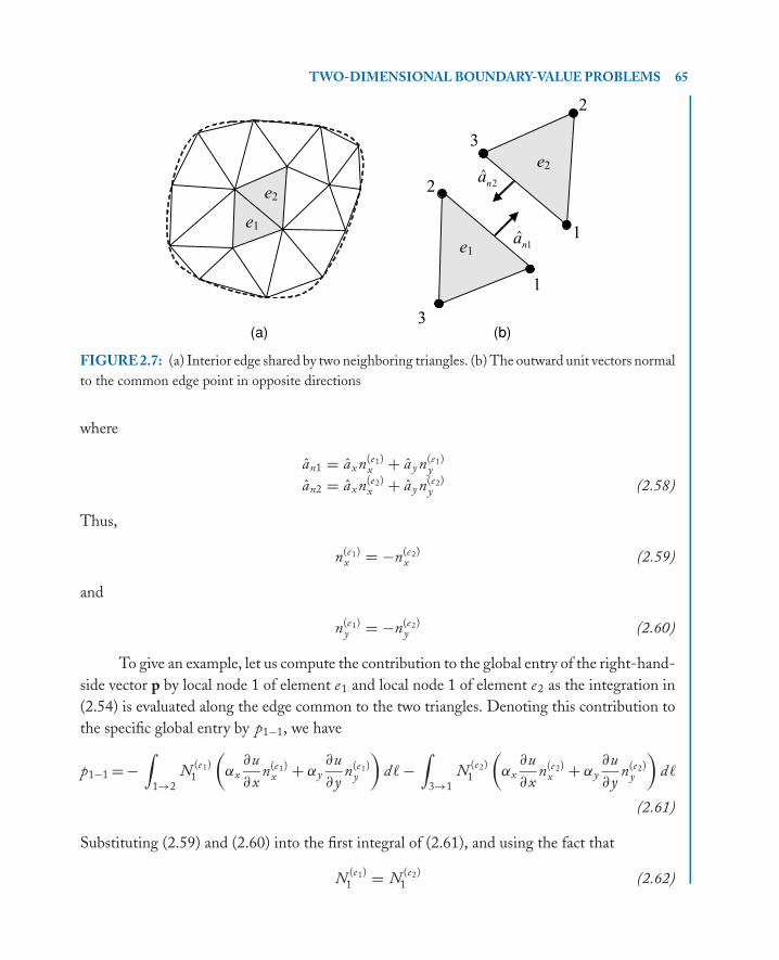
P1: IML/FFX P2: IML
MOBK021-02 MOBK021-Polycarpou.cls April 29, 2006 20:28
TWO-DIMENSIONAL BOUNDARY-VALUE PROBLEMS 65
e1
e2
(a)
e1
e2
1
1
3
2
(b)
1n
2n
2
3
a
a
FIGURE 2.7: (a) Interior edge shared by two neighboring triangles. (b) The outward unit vectors normal
to the common edge point in opposite directions
where
an1 = axn(e1)x + a y n(e1)
y
an2 = axn(e2)x + a y n(e2)
y (2.58)
Thus,
n(e1)x = −n(e2)
x (2.59)
and
n(e1)y = −n(e2)
y (2.60)
To give an example, let us compute the contribution to the global entry of the right-hand-
side vector p by local node 1 of element e1 and local node 1 of element e2 as the integration in
(2.54) is evaluated along the edge common to the two triangles. Denoting this contribution to
the specific global entry by p1−1, we have
p1−1 = −∫
1→2
N(e1)
1
(αx
∂u
∂xn(e1)
x + αy∂u
∂yn(e1)
y
)d� −
∫3→1
N(e2)
1
(αx
∂u
∂xn(e2)
x + αy∂u
∂yn(e2)
y
)d�
(2.61)
Substituting (2.59) and (2.60) into the first integral of (2.61), and using the fact that
N(e1)
1 = N(e2)
1 (2.62)
P1: IML/FFX P2: IML
MOBK021-02 MOBK021-Polycarpou.cls April 29, 2006 20:28
66 INTRODUCTION TO THE FINITE ELEMENT METHOD IN ELECTROMAGNETICS
along the path of integration, which is the common edge, it becomes evident that the two
integrals are equal in magnitude but opposite in sign, thus canceling each other out. Notice that
the line integrals in (2.61) are evaluated along the common edge and, therefore, the remaining
terms involved in the integrand of (2.54) are equal for both triangles. Similarly, the contribution
to the global entry of the right-hand-side vector p by local node 2 of element e1 and local node
3 of element e2 as the integration is evaluated along the common edge is given by
p2−3 = −∫
1→2
N(e1)2
(αx
∂u
∂xn(e1)
x + αy∂u
∂yn(e1)
y
)d� −
∫3→1
N(e2)3
(αx
∂u
∂xn(e2)
x + αy∂u
∂yn(e2)
y
)d�
(2.63)
Again, substituting (2.59) and (2.60) into the first integral of (2.63), and using the fact that
N(e1)2 = N
(e2)3 (2.64)
along the path of integration, it is evident that the two integrals cancel each other out. Conse-
quently, the contribution of the line integral in (2.54) to the global right-hand-side vector p is
zero for all interior edges. It is nonzero only for edges that belong to the domain boundary �,
where
� = �1 ∪ �2 (2.65)
For boundary edges that belong to �1, where a Dirichlet boundary condition is to be imposed,
the contribution of the line integral in (2.54) will be discarded. Thus, the only contribution of
the line integral in (2.54) is attributed only to boundary edges that reside on �2. Remember
that �2 is characterized by a mixed boundary condition of the form(αx
∂u
∂xnx + αy
∂u
∂yny
)+ γ u = q on �2 (2.66)
Rearranging the terms in (2.66) and substituting into (2.54), the line integral becomes
pei = −
∫�2
Ni (q − γ u) d� (2.67)
The line integral in (2.67) exists only for boundary elements, i.e., elements that have one or more
edges on the outer boundary of the finite element domain. Specifically, it must be evaluated only
along boundary edges that reside on �2. For interior edges, as was stated before, its contribution
is zero.
2.5 EVALUATION OF ELEMENT MATRICES AND VECTORSThe main purpose of this section is to derive analytically the expressions for the entries of all
element matrices and vectors that are present in the linear system of equations given by (2.50).
P1: IML/FFX P2: IML
MOBK021-02 MOBK021-Polycarpou.cls April 29, 2006 20:28
TWO-DIMENSIONAL BOUNDARY-VALUE PROBLEMS 67
These entry values are dependent on the type and order of interpolation functions used in the
FEM. In this section, we are going to consider two types of interpolation functions: one for
the linear triangular element, and another for the bilinear quadrilateral element. Higher order
elements will be considered separately in Section 2.11.
2.5.1 Linear Triangular Elements
We begin the evaluation of element matrices and vectors with matrix Me whose entries are
given, according to (2.51), by
Mei j = −
∫∫�e
[αx
(∂ Ni
∂x
) (∂ Nj
∂x
)+ αy
(∂ Ni
∂y
) (∂ Nj
∂y
)]d x d y (2.68)
where αx and αy are constants. At this point, it is important to remind the reader that the
governing interpolation functions for linear triangular elements are given by
N1 = 1 − ξ − η
N2 = ξ
N3 = η (2.69)
and that the x and y coordinates of any point inside an element can be expressed as
x = xe1 + x21ξ + x31η
y = ye1 + y21ξ + y31η (2.70)
where the notation
xi j = xei − xe
j (2.71)
has been used in (2.70). Using the chain rule of differentiation, one can write that
∂ N
∂ξ= ∂ N
∂x
∂x
∂ξ+ ∂ N
∂y
∂y
∂ξ
∂ N
∂η= ∂ N
∂x
∂x
∂η+ ∂ N
∂y
∂y
∂η(2.72)
In matrix form, ⎧⎪⎪⎨⎪⎪⎩∂ N
∂ξ
∂ N
∂η
⎫⎪⎪⎬⎪⎪⎭ =
⎡⎢⎢⎣∂x
∂ξ
∂y
∂ξ
∂x
∂η
∂y
∂η
⎤⎥⎥⎦⎧⎪⎪⎨⎪⎪⎩
∂ N
∂x
∂ N
∂y
⎫⎪⎪⎬⎪⎪⎭ (2.73)
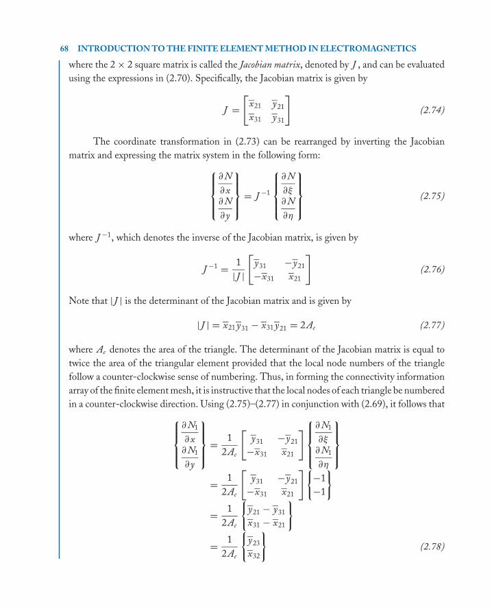
P1: IML/FFX P2: IML
MOBK021-02 MOBK021-Polycarpou.cls April 29, 2006 20:28
68 INTRODUCTION TO THE FINITE ELEMENT METHOD IN ELECTROMAGNETICS
where the 2 × 2 square matrix is called the Jacobian matrix, denoted by J , and can be evaluated
using the expressions in (2.70). Specifically, the Jacobian matrix is given by
J =[
x21 y21
x31 y31
](2.74)
The coordinate transformation in (2.73) can be rearranged by inverting the Jacobian
matrix and expressing the matrix system in the following form:⎧⎪⎪⎨⎪⎪⎩∂ N
∂x∂ N
∂y
⎫⎪⎪⎬⎪⎪⎭ = J −1
⎧⎪⎪⎨⎪⎪⎩∂ N
∂ξ∂ N
∂η
⎫⎪⎪⎬⎪⎪⎭ (2.75)
where J −1, which denotes the inverse of the Jacobian matrix, is given by
J −1 = 1
|J |
[y31 −y21
−x31 x21
](2.76)
Note that |J | is the determinant of the Jacobian matrix and is given by
|J | = x21 y31 − x31 y21 = 2Ae (2.77)
where Ae denotes the area of the triangle. The determinant of the Jacobian matrix is equal to
twice the area of the triangular element provided that the local node numbers of the triangle
follow a counter-clockwise sense of numbering. Thus, in forming the connectivity information
array of the finite element mesh, it is instructive that the local nodes of each triangle be numbered
in a counter-clockwise direction. Using (2.75)–(2.77) in conjunction with (2.69), it follows that⎧⎪⎪⎨⎪⎪⎩∂ N1
∂x∂ N1
∂y
⎫⎪⎪⎬⎪⎪⎭ = 1
2Ae
[y31 −y21
−x31 x21
] ⎧⎪⎪⎨⎪⎪⎩∂ N1
∂ξ∂ N1
∂η
⎫⎪⎪⎬⎪⎪⎭= 1
2Ae
[y31 −y21
−x31 x21
] {−1
−1
}
= 1
2Ae
{y21 − y31
x31 − x21
}
= 1
2Ae
{y23
x32
}(2.78)
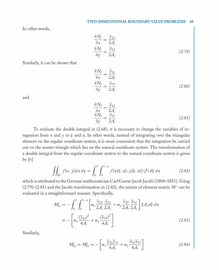
P1: IML/FFX P2: IML
MOBK021-02 MOBK021-Polycarpou.cls April 29, 2006 20:28
TWO-DIMENSIONAL BOUNDARY-VALUE PROBLEMS 69
In other words,
∂ N1
∂x= y23
2Ae
∂ N1
∂y= x32
2Ae
(2.79)
Similarly, it can be shown that
∂ N2
∂x= y31
2Ae
∂ N2
∂y= x13
2Ae
(2.80)
and
∂ N3
∂x= y12
2Ae∂ N3
∂y= x21
2Ae
(2.81)
To evaluate the double integral in (2.68), it is necessary to change the variables of in-
tegration from x and y to ξ and η. In other words, instead of integrating over the triangular
element on the regular coordinate system, it is more convenient that the integration be carried
out on the master triangle which lies on the natural coordinate system. The transformation of
a double integral from the regular coordinate system to the natural coordinate system is given
by [6] ∫∫�e
f (x, y)d x d y =∫ 1
0
∫ 1−η
0
f (x(ξ, η), y(ξ, η)) |J | dξ dη (2.82)
which is attributed to the German mathematician Carl Gustav Jacob Jacobi (1804–1851). Using
(2.79)–(2.81) and the Jacobi transformation in (2.82), the entries of element matrix M e can be
evaluated in a straightforward manner. Specifically,
Me11 = −
∫ 1
0
∫ 1−η
0
[αx
y23
2Ae
y23
2Ae
+ αyx32
2Ae
x32
2Ae
]2Ae dξ dη
= −[αx
(y23)2
4Ae
+ αy(x32)2
4Ae
](2.83)
Similarly,
Me12 = Me
21 = −[αx
y23 y31
4Ae
+ αyx32x13
4Ae
](2.84)
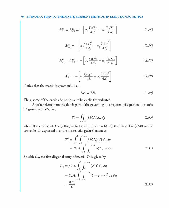
P1: IML/FFX P2: IML
MOBK021-02 MOBK021-Polycarpou.cls April 29, 2006 20:28
70 INTRODUCTION TO THE FINITE ELEMENT METHOD IN ELECTROMAGNETICS
Me13 = Me
31 = −[αx
y23 y12
4Ae
+ αyx32x21
4Ae
](2.85)
Me22 = −
[αx
(y31)2
4Ae
+ αy(x13)2
4Ae
](2.86)
Me23 = Me
32 = −[αx
y31 y12
4Ae
+ αyx13x21
4Ae
](2.87)
Me33 = −
[αx
(y12)2
4Ae
+ αy(x21)2
4Ae
](2.88)
Notice that the matrix is symmetric, i.e.,
Mei j = M e
ji (2.89)
Thus, some of the entries do not have to be explicitly evaluated.
Another element matrix that is part of the governing linear system of equations is matrix
Te given by (2.52), i.e.,
T ei j =
∫∫�e
βNi Nj d x d y (2.90)
where β is a constant. Using the Jacobi transformation in (2.82), the integral in (2.90) can be
conveniently expressed over the master triangular element as
T ei j =
∫ 1
0
∫ 1−η
0
βNi Nj |J | dξ dη
= β2Ae
∫ 1
0
∫ 1−η
0
Ni Nj dξ dη (2.91)
Specifically, the first diagonal entry of matrix T e is given by
T e11 = β2Ae
∫ 1
0
∫ 1−η
0
(N1)2 dξ dη
= β2Ae
∫ 1
0
∫ 1−η
0
(1 − ξ − η)2 dξ dη
= β Ae
6(2.92)
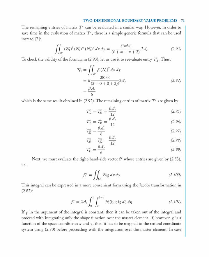
P1: IML/FFX P2: IML
MOBK021-02 MOBK021-Polycarpou.cls April 29, 2006 20:28
TWO-DIMENSIONAL BOUNDARY-VALUE PROBLEMS 71
The remaining entries of matrix T e can be evaluated in a similar way. However, in order to
save time in the evaluation of matrix T e , there is a simple generic formula that can be used
instead [7]: ∫∫�e
(N1)� (N2)m (N3)n d x d y = �!m!n!
(� + m + n + 2)!2Ae (2.93)
To check the validity of the formula in (2.93), let us use it to reevaluate entry T e11. Thus,
T e11 =
∫∫�e
β (N1)2 d x d y
= β2!0!0!
(2 + 0 + 0 + 2)!2Ae (2.94)
= β Ae
6
which is the same result obtained in (2.92). The remaining entries of matrix T e are given by
T e12 = T e
21 = β Ae
12(2.95)
T e13 = T e
31 = β Ae
12(2.96)
T e22 = β Ae
6(2.97)
T e23 = T e
32 = β Ae
12(2.98)
T e33 = β Ae
6(2.99)
Next, we must evaluate the right-hand-side vector f e whose entries are given by (2.53),
i.e.,
f ei =
∫∫�e
Ni g d x d y (2.100)
This integral can be expressed in a more convenient form using the Jacobi transformation in
(2.82):
f ei = 2Ae
∫ 1
0
∫ 1−η
0
Ni (ξ, η)g dξ dη (2.101)
If g in the argument of the integral is constant, then it can be taken out of the integral and
proceed with integrating only the shape function over the master element. If, however, g is a
function of the space coordinates x and y , then it has to be mapped to the natural coordinate
system using (2.70) before proceeding with the integration over the master element. In case

P1: IML/FFX P2: IML
MOBK021-02 MOBK021-Polycarpou.cls April 29, 2006 20:28
72 INTRODUCTION TO THE FINITE ELEMENT METHOD IN ELECTROMAGNETICS
the integration is difficult to be evaluated analytically, it may be more convenient to evaluate it
numerically. Here, it is assumed that g is constant inside the integral and, thus, the entries of
the right-hand-side vector f e are given, according to (2.93), by
f e1 = g
∫∫�e
N1dx dy = g1!0!0!
(1 + 0 + 0 + 2)!2Ae = g Ae
3
f e2 = g
∫∫�e
N2dx dy = g0!1!0!
(0 + 1 + 0 + 2)!2Ae = g Ae
3(2.102)
f e3 = g
∫∫�e
N3dx dy = g0!0!1!
(0 + 0 + 1 + 2)!2Ae = g Ae
3
At last, we must evaluate the right-hand-side vector pe whose entries are given by (2.54).
Note that (2.54) reduces to (2.67) after imposing the mixed boundary condition in (2.66). Thus,
the ith entry of the element vector pe is given by
pei = −
∫�2
Ni (q − γ u) d� (2.103)
where q and γ are constants. The integral in (2.103) is nonzero only for boundary elements that
have at least one edge coinciding with �2 and where either q or γ is nonzero; if both q and γ
are zero, then automatically the integral in (2.103) becomes zero. For example, to impose a
Neumann boundary condition on �2, q and γ must be set to zero. This is equivalent to having
a right-hand-side vector pe equal to the zero vector 0. Now, for a generic mixed boundary
condition, as given by (2.66), with nonzero q and γ , the integral in (2.103) becomes
pei = −
∫Le
b
Ni
(q − γ
3∑j=1
uej Nj
)d�
= −∫
Leb
Ni q d� +∫
Leb
Niγ(ue
1 N1 + ue2 N2 + ue
3 N3
)d�
(2.104)
where Leb denotes the boundary edge of the element that coincides with �2.
Consider the triangular element illustrated in Figure 2.8(a) with one edge lying on �2.
Numbering the local nodes of the element as indicated in the figure, the integral in (2.104)
must be evaluated along the edge from node 1 to node 2 (1 → 2). In other words,
pei = −
∫1→2
Ni q d� +∫
1→2
Niγ(ue
1 N1 + ue2 N2 + ue
3 N3
)d� (2.105)
To evaluate the integral in (2.105), triangle e must be mapped onto the master triangle in the
natural coordinate system, as shown in Figure 2.8(b). Thus, integrating along edge 1 → 2 on
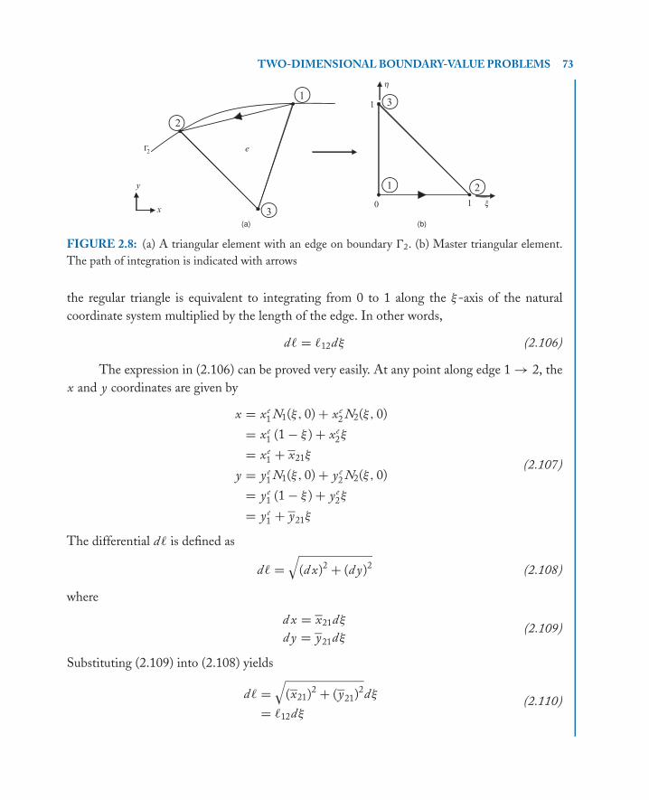
P1: IML/FFX P2: IML
MOBK021-02 MOBK021-Polycarpou.cls April 29, 2006 20:28
TWO-DIMENSIONAL BOUNDARY-VALUE PROBLEMS 73
FIGURE 2.8: (a) A triangular element with an edge on boundary �2. (b) Master triangular element.
The path of integration is indicated with arrows
the regular triangle is equivalent to integrating from 0 to 1 along the ξ-axis of the natural
coordinate system multiplied by the length of the edge. In other words,
d� = �12dξ (2.106)
The expression in (2.106) can be proved very easily. At any point along edge 1 → 2, the
x and y coordinates are given by
x = xe1 N1(ξ, 0) + xe
2 N2(ξ, 0)
= xe1 (1 − ξ ) + xe
2ξ
= xe1 + x21ξ
y = ye1 N1(ξ, 0) + ye
2 N2(ξ, 0)
= ye1 (1 − ξ ) + ye
2ξ
= ye1 + y21ξ
(2.107)
The differential d� is defined as
d� =√
(d x)2 + (d y)2 (2.108)
where
d x = x21dξ
d y = y21dξ(2.109)
Substituting (2.109) into (2.108) yields
d� =√
(x21)2 + (y21)2dξ
= �12dξ(2.110)

P1: IML/FFX P2: IML
MOBK021-02 MOBK021-Polycarpou.cls April 29, 2006 20:28
74 INTRODUCTION TO THE FINITE ELEMENT METHOD IN ELECTROMAGNETICS
Thus, using the result of (2.106), the integral in (2.105), evaluated for local node 1 of the
element, becomes
pe1 = −
∫ 1
0
N1(ξ, 0)q�12dξ
+∫ 1
0
N1(ξ, 0)γ[ue
1 N1(ξ, 0) + ue2 N2(ξ, 0) + ue
3 N3(ξ, 0)]�12dξ
= −∫ 1
0
(1 − ξ ) q �12dξ +∫ 1
0
(1 − ξ ) γ[ue
1 (1 − ξ ) + ue2ξ + ue
3 0]�12dξ
= −q�12
2+
[γ �12
3ue
1 + γ �12
6ue
2 + 0 ue3
](2.111)
The terms enclosed in the square brackets must be transferred to the left-hand side of the
element matrix system in (2.55). This is equivalent to subtracting the coefficients of ue1, ue
2, and
ue3 from the matrix entries K e
11, K e12, and K e
13, respectively, i.e.,
K e11 = K e
11 − γ �12
3
K e12 = K e
12 − γ �12
6(2.112)
K e13 = K e
13 − 0
Similarly, the vector entry that corresponds to local node 2 is given, according to the integral
in (2.105), by
pe2 = −
∫ 1
0
N2(ξ, 0)q�12dξ
+∫ 1
0
N2(ξ, 0)γ[ue
1 N1(ξ, 0) + ue2 N2(ξ, 0) + ue
3 N3(ξ, 0)]�12dξ
= −∫ 1
0
ξ q �12dξ +∫ 1
0
ξ γ[ue
1 (1 − ξ ) + ue2ξ + ue
30]�12dξ
= −q�12
2+
[γ �12
6ue
1 + γ �12
3ue
2 + 0 ue3
](2.113)
Again, the terms within the square brackets must be transferred to the left-hand side of the
element matrix system and be subtracted from the entries of matrix K e ; i.e.,
K e21 = K e
21 − γ �12
6
K e22 = K e
22 − γ �12
3(2.114)
K e23 = K e
33 − 0
P1: IML/FFX P2: IML
MOBK021-02 MOBK021-Polycarpou.cls April 29, 2006 20:28
TWO-DIMENSIONAL BOUNDARY-VALUE PROBLEMS 75
Finally, the vector entry that corresponds to local node 3 is
pe3 = −
∫ 1
0
N3(ξ, 0)q�12dξ
+∫ 1
0
N3(ξ, 0)γ[ue
1 N1(ξ, 0) + ue2 N2(ξ, 0) + ue
3 N3(ξ, 0)]�12dξ
= 0
(2.115)
due to the fact that N3 (ξ, 0) = 0 along the ξ-axis. The element right-hand-side vector pe for
a boundary element locally numbered as shown in Figure 2.8(a) is therefore given by
pe = −q�12
2
⎧⎪⎨⎪⎩1
1
0
⎫⎪⎬⎪⎭ (2.116)
Exercise 2.2. Given a linear triangular element on the xy-plane whose nodes are numbered in
a counter-clockwise direction, prove that the determinant of the Jacobian matrix is twice the
area of the triangle.
Exercise 2.3. Using the Jacobi transformation, evaluate the double integral in (2.68) to show
that the entries of matrix Me are given by (2.83)–(2.88). Follow the same procedure as was done
for Me11. Repeat the exercise for matrix T e to show that its entries are given by (2.94)–(2.99).
2.5.2 Bilinear Quadrilateral Elements
The evaluation of element matrices and vectors using bilinear quadrilateral elements follows
the same step-by-step procedure as the one used for linear triangular elements. The governing
interpolation functions for a bilinear quadrilateral element are given by
N1 = 1
4(1 − ξ )(1 − η)
N2 = 1
4(1 + ξ )(1 − η)
N3 = 1
4(1 + ξ )(1 + η)
N4 = 1
4(1 − ξ )(1 + η)
(2.117)
Using an isoparametric representation, the x, y space coordinates of a point inside a quadrilateral
and the primary unknown quantity are expanded in terms of the same interpolation functions,
i.e.,
x = xe1 N1 + xe
2 N2 + xe3 N3 + xe
4 N4
y = ye1 N1 + ye
2 N2 + ye3 N3 + ye
4 N4
(2.118)
P1: IML/FFX P2: IML
MOBK021-02 MOBK021-Polycarpou.cls April 29, 2006 20:28
76 INTRODUCTION TO THE FINITE ELEMENT METHOD IN ELECTROMAGNETICS
and
u = ue1 N1 + ue
2 N2 + ue3 N3 + ue
4 N4 (2.119)
where xei , ye
i for i = 1,2,3,4 are the node coordinates of the quadrilateral element, and uei for
i = 1,2,3,4 are the values of the primary unknown quantity at the four nodes. Using the chain
rule of differentiation, the partial derivatives of the interpolation functions in (2.117) with
respect to ξ and η can be expressed as
∂ Ni
∂ξ= ∂ Ni
∂x
∂x
∂ξ+ ∂ Ni
∂y
∂y
∂ξ
∂ Ni
∂η= ∂ Ni
∂x
∂x
∂η+ ∂ Ni
∂y
∂y
∂η
(2.120)
or in a more convenient matrix form⎧⎪⎪⎨⎪⎪⎩∂ Ni
∂ξ
∂ Ni
∂η
⎫⎪⎪⎬⎪⎪⎭ =
⎡⎢⎢⎣∂x
∂ξ
∂y
∂ξ
∂x
∂η
∂y
∂η
⎤⎥⎥⎦⎧⎪⎪⎨⎪⎪⎩
∂ Ni
∂x∂ Ni
∂y
⎫⎪⎪⎬⎪⎪⎭= J
⎧⎪⎨⎪⎩∂ Ni
∂x∂ Ni
∂y
⎫⎪⎬⎪⎭(2.121)
where J , the Jacobian matrix, is given by
J =[
J11 J12
J21 J22
](2.122)
with
J11 = 1
4
[− (1 − η) xe1 + (1 − η) xe
2 + (1 + η) xe3 − (1 + η) xe
4
]J12 = 1
4
[− (1 − η) ye1 + (1 − η) ye
2 + (1 + η) ye3 − (1 + η) ye
4
]J21 = 1
4
[− (1 − ξ ) xe1 − (1 + ξ ) xe
2 + (1 + ξ ) xe3 + (1 − ξ ) xe
4
]J22 = 1
4
[− (1 − ξ ) ye1 − (1 + ξ ) ye
2 + (1 + ξ ) ye3 + (1 − ξ ) ye
4
](2.123)
P1: IML/FFX P2: IML
MOBK021-02 MOBK021-Polycarpou.cls April 29, 2006 20:28
TWO-DIMENSIONAL BOUNDARY-VALUE PROBLEMS 77
To express the partial derivatives with respect to x and y in terms of the partial derivatives
with respect to ξ and η, the Jacobian matrix must be inverted, i.e.,⎧⎪⎨⎪⎩∂ Ni
∂x∂ Ni
∂y
⎫⎪⎬⎪⎭ = J −1
⎧⎪⎪⎨⎪⎪⎩∂ Ni
∂ξ
∂ Ni
∂η
⎫⎪⎪⎬⎪⎪⎭= 1
|J |
[J22 −J12
−J21 J11
] ⎧⎪⎪⎨⎪⎪⎩∂ Ni
∂ξ
∂ Ni
∂η
⎫⎪⎪⎬⎪⎪⎭(2.124)
where |J | is the determinant of the Jacobian matrix given by
|J | = J11 J22 − J12 J21 (2.125)
As an example, let us consider the interpolation function that corresponds to node 1:
∂ N1
∂ξ= −1
4(1 − η)
∂ N1
∂η= −1
4(1 − ξ )
(2.126)
Substituting (2.126) into (2.124), we have⎧⎪⎨⎪⎩∂ N1
∂x∂ N1
∂y
⎫⎪⎬⎪⎭ = 1
|J |
[J22 −J12
−J21 J11
] {− 1
4(1 − η)
− 14(1 − ξ )
}(2.127)
which can also be written as
∂ N1
∂x= 1
4 |J | [−J22(1 − η) + J12(1 − ξ )]
∂ N1
∂y= 1
4 |J | [J21(1 − η) − J11(1 − ξ )]
(2.128)
Similarly, it can be shown that
∂ N2
∂x= 1
4 |J | [J22(1 − η) + J12(1 + ξ )]
∂ N2
∂y= 1
4 |J | [−J21(1 − η) − J11(1 + ξ )]
(2.129)

P1: IML/FFX P2: IML
MOBK021-02 MOBK021-Polycarpou.cls April 29, 2006 20:28
78 INTRODUCTION TO THE FINITE ELEMENT METHOD IN ELECTROMAGNETICS
∂ N3
∂x= 1
4 |J | [J22(1 + η) − J12(1 + ξ )]
∂ N3
∂y= 1
4 |J | [−J21(1 + η) + J11(1 + ξ )]
(2.130)
∂ N4
∂x= 1
4 |J | [−J22(1 + η) − J12(1 − ξ )]
∂ N4
∂y= 1
4 |J | [J21(1 + η) + J11(1 − ξ )]
(2.131)
The first matrix to be evaluated, on an element basis, is Me . The entries of this matrix
are given by
Mei j = −
∫∫�e
[αx
∂ Ni
∂x
∂ Nj
∂x+ αy
∂ Ni
∂y
∂ Nj
∂y
]d x d y (2.132)
where �e is the domain of the quadrilateral element. Using the Jacobi transformation introduced
for triangular elements in (2.82), modified however for quadrilateral elements, the integral in
(2.132) can be expressed in a more convenient form given by
Mei j = −
∫ 1
−1
∫ 1
−1
[αx
∂ Ni
∂x
∂ Nj
∂x+ αy
∂ Ni
∂y
∂ Nj
∂y
]|J | dξ dη (2.133)
As seen, the double integral is now evaluated over the domain of the master element which
corresponds to a square [see Figure 2.6(b)]. Notice that the partial derivatives of the governing
interpolation functions with respect to x and y were conveniently expressed using the Jacobian
matrix in terms of the natural coordinates ξ and η. These expressions are given by (2.128)–
(2.131).
As an example, let us evaluate entry Me11:
Me11 = −
∫ 1
−1
∫ 1
−1
[αx
(∂ N1
∂x
)2
+ αy
(∂ N1
∂y
)2]
|J | dξ dη
= − 1
16
∫ 1
−1
∫ 1
−1
1
|J |
{αx [−J22 (1 − η) + J12 (1 − ξ )]2 +αy [J21 (1 − η) − J11 (1 − ξ )]2
}dξ dη
(2.134)
Unlike the case of using linear triangular elements, the integrand of (2.134) is a fairly complex
function of ξ and η, which makes the integral difficult to evaluate analytically. This integral
must be evaluated numerically. Although there are many numerical methods [8, 9] that can be
used to evaluate a double integration, some of which include midpoint rule and trapezoid rule,
the most appropriate and widely used approach in the FEM is Gauss quadrature.
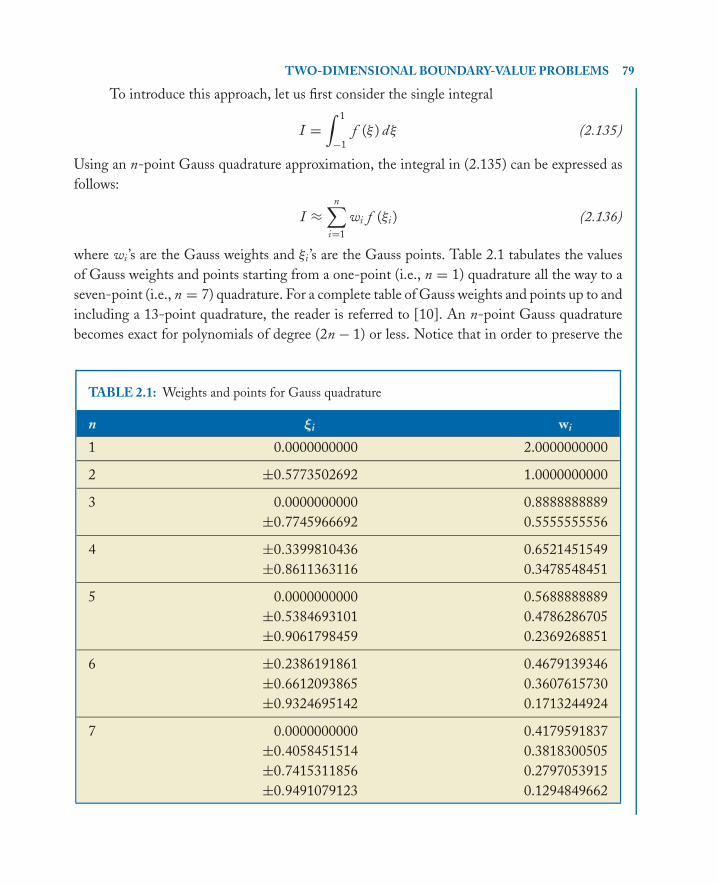
P1: IML/FFX P2: IML
MOBK021-02 MOBK021-Polycarpou.cls April 29, 2006 20:28
TWO-DIMENSIONAL BOUNDARY-VALUE PROBLEMS 79
To introduce this approach, let us first consider the single integral
I =∫ 1
−1
f (ξ ) dξ (2.135)
Using an n-point Gauss quadrature approximation, the integral in (2.135) can be expressed as
follows:
I ≈n∑
i=1
wi f (ξi ) (2.136)
where wi ’s are the Gauss weights and ξi ’s are the Gauss points. Table 2.1 tabulates the values
of Gauss weights and points starting from a one-point (i.e., n = 1) quadrature all the way to a
seven-point (i.e., n = 7) quadrature. For a complete table of Gauss weights and points up to and
including a 13-point quadrature, the reader is referred to [10]. An n-point Gauss quadrature
becomes exact for polynomials of degree (2n − 1) or less. Notice that in order to preserve the
TABLE 2.1: Weights and points for Gauss quadrature
n ξi wi
1 0.0000000000 2.0000000000
2 ±0.5773502692 1.0000000000
3 0.0000000000 0.8888888889
±0.7745966692 0.5555555556
4 ±0.3399810436 0.6521451549
±0.8611363116 0.3478548451
5 0.0000000000 0.5688888889
±0.5384693101 0.4786286705
±0.9061798459 0.2369268851
6 ±0.2386191861 0.4679139346
±0.6612093865 0.3607615730
±0.9324695142 0.1713244924
7 0.0000000000 0.4179591837
±0.4058451514 0.3818300505
±0.7415311856 0.2797053915
±0.9491079123 0.1294849662

P1: IML/FFX P2: IML
MOBK021-02 MOBK021-Polycarpou.cls April 29, 2006 20:28
80 INTRODUCTION TO THE FINITE ELEMENT METHOD IN ELECTROMAGNETICS
accuracy of Gauss quadrature rule, a large number of significant figures must be considered
when storing the Gauss weights and points in a computer. It is also recommended that double
precision arithmetic be used when implementing Gauss quadrature in a computer code.
Gauss quadrature can also be applied to double integrals of the form
I =∫ 1
−1
∫ 1
−1
f (ξ, η) dξdη (2.137)
Employing an n-point Gauss quadrature approximation, one can write that
I ≈∫ 1
−1
[n∑
i=1
wi f (ξi , η)
]dη
≈n∑
j=1
w j
[n∑
i=1
wi f(ξi , η j
)]
≈n∑
j=1
n∑i=1
wi w j f(ξi , η j
)(2.138)
Similarly, Gauss quadrature can be extended to volume integrals over a cube. It is important,
however, to emphasize here that Gauss weights and points for triangles are different from the
ones tabulated in Table 2.1. For more information on Gauss quadrature for triangular domains,
refer to [10, 11].
Now that the reader has become familiar with Gauss quadrature, the integral in (2.134) can
be evaluated numerically using (2.138) and the data posted in Table 2.1. The second element ma-
trix involved in the 2-D nodal finite element formulation is matrix Te whose entries are given by
Tei j =
∫∫�e
βNi Nj d x d y
=∫ 1
−1
∫ 1
−1
βNi Nj |J | dξ dη
(2.139)
As with matrix M e , the integrand involved in matrix T e is also complex and that makes it
extremely difficult to integrate analytically. Thus, choosing the appropriate n-point Gauss
quadrature, depending on the degree of the polynomial involved, the integral in (2.139) can
be evaluated numerically.
As an example, entry T e11 becomes
T e11 ≈
n∑j=1
n∑i=1
wi w jβ[
N1
(ξi , η j
)]2 ∣∣J(ξi , η j
)∣∣ (2.140)
where n must be such that the degree of the polynomial involved in the integrand is (2n − 1)
or less. The remaining entries of matrix T e are evaluated in a similar way. In addition, the
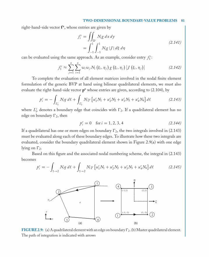
P1: IML/FFX P2: IML
MOBK021-02 MOBK021-Polycarpou.cls April 29, 2006 20:28
TWO-DIMENSIONAL BOUNDARY-VALUE PROBLEMS 81
right-hand-side vector f e, whose entries are given by
f ei =
∫∫�e
Ni g d x d y
=∫ 1
−1
∫ 1
−1
Ni g |J | dξ dη
(2.141)
can be evaluated using the same approach. As an example, consider entry f e1 :
f e1 ≈
n∑j=1
n∑i=1
wi w j N1
(ξi , η j
)g
(ξi , η j
) ∣∣J(ξi , η j
)∣∣ (2.142)
To complete the evaluation of all element matrices involved in the nodal finite element
formulation of the generic BVP at hand using bilinear quadrilateral elements, we must also
evaluate the right-hand-side vector pe whose entries are given, according to (2.104), by
pei = −
∫Le
b
Ni q d� +∫
Leb
Niγ[ue
1 N1 + ue2 N2 + ue
3 N3 + ue4 N4
]d� (2.143)
where Leb denotes a boundary edge that coincides with �2. If a quadrilateral element has no
edge on boundary �2, then
pei = 0 for i = 1, 2, 3, 4 (2.144)
If a quadrilateral has one or more edges on boundary �2, the two integrals involved in (2.143)
must be evaluated along each of these boundary edges. To illustrate how these two integrals are
evaluated, consider the boundary quadrilateral element shown in Figure 2.9(a) with one edge
lying on �2.
Based on this figure and the associated nodal numbering scheme, the integral in (2.143)
becomes
pei = −
∫1→2
Ni q d� +∫
1→2
Niγ[ue
1 N1 + ue2 N2 + ue
3 N3 + ue4 N4
]d� (2.145)
e
1
2
3
2
4
1 (–1,–1)
x
y
(a) (b)4
2
3
(1,–1)
(1,1) (–1,1)
x
h
Γ
FIGURE2.9: (a) A quadrilateral element with an edge on boundary �2. (b) Master quadrilateral element.
The path of integration is indicated with arrows

P1: IML/FFX P2: IML
MOBK021-02 MOBK021-Polycarpou.cls April 29, 2006 20:28
82 INTRODUCTION TO THE FINITE ELEMENT METHOD IN ELECTROMAGNETICS
Evaluation of the integral in (2.145) requires that quadrilateral e in Figure 2.9(a) be mapped
onto the master element shown in Figure 2.9(b). Doing that, the integral in (2.145) can be
equivalently expressed as
pei = −�12
2
∫ 1
−1
Ni (ξ, −1)q dξ + �12
2
∫ 1
−1
Ni (ξ, −1)γ
[ue
1 N1(ξ, −1) + ue2 N2(ξ, −1)+
ue3 N3(ξ, −1) + ue
4 N4(ξ, −1)
]dξ
(2.146)
Notice that integrating along edge 1 → 2 is equivalent to integrating on the natural coordinate
system along the ξ-axis from ξ = −1 to ξ = 1 with d� replaced by
d� = �12
2dξ (2.147)
The expression in (2.147) can be derived fairly easily once we realize that along edge 1 → 2 the
natural coordinate η = −1; i.e.,
x = xe1 N1(ξ, −1) + xe
2 N2(ξ, −1) + xe3 N3(ξ, −1) + xe
4 N4(ξ, −1)
= xe1
1
2(1 − ξ ) + xe
2
1
2(1 + ξ ) + xe
30 + xe40
=(
xe1 + xe
2
2
)+
(xe
2 − xe1
2
)ξ
(2.148)
Similarly, it can be shown that
y =(
ye1 + ye
2
2
)+
(ye
2 − ye1
2
)ξ (2.149)
The differential d� is given by
d� =√
(d x)2 + (d y)2 (2.150)
where
d x = xe2 − xe
1
2dξ = x21
2dξ
d y = ye2 − ye
1
2dξ = y21
2dξ
(2.151)
Substituting (2.151) into (2.150) yields
d� = 1
2
√(x21)2 + (y21)2dξ
= �12
2dξ
(2.152)
P1: IML/FFX P2: IML
MOBK021-02 MOBK021-Polycarpou.cls April 29, 2006 20:28
TWO-DIMENSIONAL BOUNDARY-VALUE PROBLEMS 83
Now, let us evaluate (2.146) for i = 1, 2, 3, and 4 assuming q and γ are constants.
Specifically, for i = 1,
pe1 = −�12
2
∫ 1
−1
N1(ξ, −1)q dξ + �12
2
∫ 1
−1
N1(ξ, −1)γ
[ue
1 N1(ξ, −1) + ue2 N2(ξ, −1)+
ue3 N3(ξ, −1) + ue
4 N4(ξ, −1)
]dξ
= −�12q
4
∫ 1
−1
(1 − ξ ) dξ + �12q
8
∫ 1
−1
(1 − ξ )[ue
1 (1 − ξ ) + ue2 (1 + ξ ) + ue
30 + ue40
]dξ
= −�12q
2+
[γ �12
3ue
1 + γ �12
12ue
2 + 0 ue3 + 0 ue
4
](2.153)
As was done in the case of triangular elements, the terms enclosed in the square brackets
must be transferred to the left-hand side of the element matrix in (2.55). This is equivalent to
subtracting the coefficients of ue1, ue
2, ue3, and ue
4 from the matrix entries K e11, K e
12, K e13, and
K e14, respectively, i.e.,
K e11 = K e
11 − γ �12
3
K e12 = K e
12 − γ �12
12(2.154)
K e13 = K e
13 − 0
K e14 = K e
14 − 0
Similarly,
pe2 = −�12q
2+
[γ �12
12ue
1 + γ �12
3ue
2 + 0 ue3 + 0 ue
4
](2.155)
Again, the terms inside the square brackets must be transferred to the left-hand side of the
element matrix system and be subtracted from the entries of matrix K e ; i.e.,
K e21 = K e
21 − γ �12
12
K e22 = K e
22 − γ �12
3(2.156)
K e23 = K e
23 − 0
K e24 = K e
24 − 0
The other two entries of vector pe are zero since
N3(ξ, −1) = 0
N4(ξ, −1) = 0(2.157)
P1: IML/FFX P2: IML
MOBK021-02 MOBK021-Polycarpou.cls April 29, 2006 20:28
84 INTRODUCTION TO THE FINITE ELEMENT METHOD IN ELECTROMAGNETICS
Thus, for the quadrilateral element on boundary �2 depicted in Figure 2.9(a), the right-hand-
side vector pe is given by
pe = −�12q
2
⎧⎪⎪⎪⎨⎪⎪⎪⎩1
1
0
0
⎫⎪⎪⎪⎬⎪⎪⎪⎭ (2.158)
It is important to point out here that for every element with one edge on boundary �2,
the corresponding entries of matrix K e must be updated according to (2.154) and (2.156). This
is equivalent to updating the entries of matrix K e once for every edge on boundary �2. In other
words, for edge 1 → 2, the relevant entries of matrix K e must be updated according to
K e11 = K e
11 − γ �12
3
K e12 = K e
12 − γ �12
12
K e21 = K e
21 − γ �12
12
K e22 = K e
22 − γ �12
3
(2.159)
which results after combining (2.154) and (2.156). If the edge on boundary �2 is defined by
local node numbers 2 and 3, the matrix update must occur on entries K e22, K e
23, K e32, and K e
33
instead of K e11, K e
12, K e21, and K e
22. Furthermore, the right-hand-side vector pe would be given
by
pe = −�23q
2
⎧⎪⎪⎪⎨⎪⎪⎪⎩0
1
1
0
⎫⎪⎪⎪⎬⎪⎪⎪⎭ (2.160)
Now, if the element has two edges on boundary �2, as shown in Figure 2.10, the corre-
sponding vector pe will take the form
pe = −�12q
2
⎧⎪⎪⎪⎨⎪⎪⎪⎩1
1
0
0
⎫⎪⎪⎪⎬⎪⎪⎪⎭ − �23q
2
⎧⎪⎪⎪⎨⎪⎪⎪⎩0
1
1
0
⎫⎪⎪⎪⎬⎪⎪⎪⎭ (2.161)
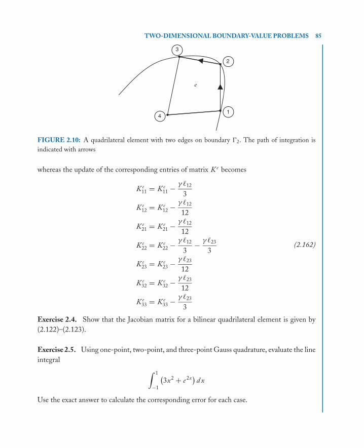
P1: IML/FFX P2: IML
MOBK021-02 MOBK021-Polycarpou.cls April 29, 2006 20:28
TWO-DIMENSIONAL BOUNDARY-VALUE PROBLEMS 85
e
2
1
3
4
FIGURE 2.10: A quadrilateral element with two edges on boundary �2. The path of integration is
indicated with arrows
whereas the update of the corresponding entries of matrix K e becomes
K e11 = K e
11 − γ �12
3
K e12 = K e
12 − γ �12
12
K e21 = K e
21 − γ �12
12
K e22 = K e
22 − γ �12
3− γ �23
3
K e23 = K e
23 − γ �23
12
K e32 = K e
32 − γ �23
12
K e33 = K e
33 − γ �23
3
(2.162)
Exercise 2.4. Show that the Jacobian matrix for a bilinear quadrilateral element is given by
(2.122)–(2.123).
Exercise 2.5. Using one-point, two-point, and three-point Gauss quadrature, evaluate the line
integral ∫ 1
−1
(3x2 + e 2x
)d x
Use the exact answer to calculate the corresponding error for each case.
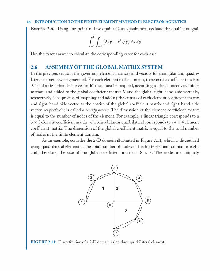
P1: IML/FFX P2: IML
MOBK021-02 MOBK021-Polycarpou.cls April 29, 2006 20:28
86 INTRODUCTION TO THE FINITE ELEMENT METHOD IN ELECTROMAGNETICS
Exercise 2.6. Using one-point and two-point Gauss quadrature, evaluate the double integral∫ 1
−1
∫ 1
−1
(2xy − x2√y
)d x d y
Use the exact answer to calculate the corresponding error for each case.
2.6 ASSEMBLY OF THE GLOBAL MATRIX SYSTEMIn the previous section, the governing element matrices and vectors for triangular and quadri-
lateral elements were generated. For each element in the domain, there exist a coefficient matrix
K e and a right-hand-side vector be that must be mapped, according to the connectivity infor-
mation, and added to the global coefficient matrix K and the global right-hand-side vector b,
respectively. The process of mapping and adding the entries of each element coefficient matrix
and right-hand-side vector to the entries of the global coefficient matrix and right-hand-side
vector, respectively, is called assembly process. The dimension of the element coefficient matrix
is equal to the number of nodes of the element. For example, a linear triangle corresponds to a
3 × 3 element coefficient matrix, whereas a bilinear quadrilateral corresponds to a 4 × 4 element
coefficient matrix. The dimension of the global coefficient matrix is equal to the total number
of nodes in the finite element domain.
As an example, consider the 2-D domain illustrated in Figure 2.11, which is discretized
using quadrilateral elements. The total number of nodes in the finite element domain is eight
and, therefore, the size of the global coefficient matrix is 8 × 8. The nodes are uniquely
1 2
3
1
2
3
4
5
6
7
8
FIGURE 2.11: Discretization of a 2-D domain using three quadrilateral elements
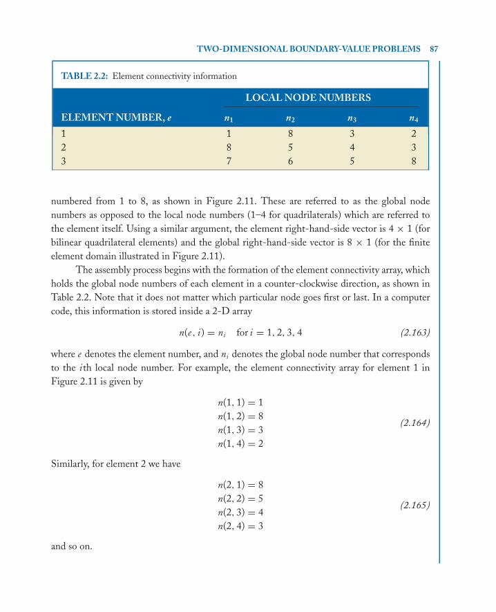
P1: IML/FFX P2: IML
MOBK021-02 MOBK021-Polycarpou.cls April 29, 2006 20:28
TWO-DIMENSIONAL BOUNDARY-VALUE PROBLEMS 87
TABLE 2.2: Element connectivity information
LOCAL NODE NUMBERS
ELEMENT NUMBER, e n1 n2 n3 n4
1 1 8 3 2
2 8 5 4 3
3 7 6 5 8
numbered from 1 to 8, as shown in Figure 2.11. These are referred to as the global node
numbers as opposed to the local node numbers (1–4 for quadrilaterals) which are referred to
the element itself. Using a similar argument, the element right-hand-side vector is 4 × 1 (for
bilinear quadrilateral elements) and the global right-hand-side vector is 8 × 1 (for the finite
element domain illustrated in Figure 2.11).
The assembly process begins with the formation of the element connectivity array, which
holds the global node numbers of each element in a counter-clockwise direction, as shown in
Table 2.2. Note that it does not matter which particular node goes first or last. In a computer
code, this information is stored inside a 2-D array
n(e , i) = ni for i = 1, 2, 3, 4 (2.163)
where e denotes the element number, and ni denotes the global node number that corresponds
to the ith local node number. For example, the element connectivity array for element 1 in
Figure 2.11 is given by
n(1, 1) = 1
n(1, 2) = 8
n(1, 3) = 3
n(1, 4) = 2
(2.164)
Similarly, for element 2 we have
n(2, 1) = 8
n(2, 2) = 5
n(2, 3) = 4
n(2, 4) = 3
(2.165)
and so on.

P1: IML/FFX P2: IML
MOBK021-02 MOBK021-Polycarpou.cls April 29, 2006 20:28
88 INTRODUCTION TO THE FINITE ELEMENT METHOD IN ELECTROMAGNETICS
Once the element connectivity array is formed, an 8 × 8 global matrix is created with its
entries initialized to zero. Thus, initially the global coefficient matrix is a null matrix
K =
⎡⎢⎢⎢⎢⎢⎢⎢⎢⎢⎢⎢⎢⎣
0 0 0 0 0 0 0 0
0 0 0 0 0 0 0 0
0 0 0 0 0 0 0 0
0 0 0 0 0 0 0 0
0 0 0 0 0 0 0 0
0 0 0 0 0 0 0 0
0 0 0 0 0 0 0 0
0 0 0 0 0 0 0 0
⎤⎥⎥⎥⎥⎥⎥⎥⎥⎥⎥⎥⎥⎦(2.166)
The process of assembly begins by looping through all the elements one-by-one and updating
the entries of the global coefficient matrix according to the following Matlab algorithm:
for e=1:3 % loop through the elements in the domain
for i=1:4 % loop through the local nodes (1st loop) of element e
for j=1:4 % loop through the local nodes (2nd loop) of element e
K(n(e,i),n(e,j)) = K(n(e,i),n(e,j)) + ke(i,j);
end
end
end
where K denotes the global coefficient matrix and ke denotes the element coefficient matrix.
By completing the assembly of element 1, the global coefficient matrix has the following form:
K =
⎡⎢⎢⎢⎢⎢⎢⎢⎢⎢⎢⎢⎢⎢⎢⎢⎣
K (1)11 K
(1)14 K
(1)13 0 0 0 0 K
(1)12
K(1)41 K
(1)44 K
(1)43 0 0 0 0 K
(1)42
K(1)31 K
(1)34 K
(1)33 0 0 0 0 K
(1)32
0 0 0 0 0 0 0 0
0 0 0 0 0 0 0 0
0 0 0 0 0 0 0 0
0 0 0 0 0 0 0 0
K(1)21 K
(1)24 K
(1)23 0 0 0 0 K
(1)22
⎤⎥⎥⎥⎥⎥⎥⎥⎥⎥⎥⎥⎥⎥⎥⎥⎦(2.167)
In other words, according to the element connectivity information in Table 2.2, element entry
K(1)23 maps to global entry K83, element entry K
(1)42 maps to global entry K28, and so on. It is also
worth noting here that the matrix in (2.167) is symmetric about the main diagonal. This can be
deduced directly from the integrals describing each entry in the weak formulation of the problem.
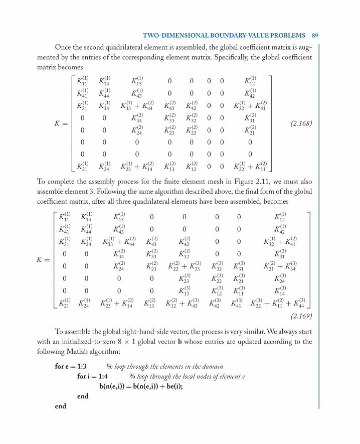
P1: IML/FFX P2: IML
MOBK021-02 MOBK021-Polycarpou.cls April 29, 2006 20:28
TWO-DIMENSIONAL BOUNDARY-VALUE PROBLEMS 89
Once the second quadrilateral element is assembled, the global coefficient matrix is aug-
mented by the entries of the corresponding element matrix. Specifically, the global coefficient
matrix becomes
K =
⎡⎢⎢⎢⎢⎢⎢⎢⎢⎢⎢⎢⎢⎢⎢⎢⎢⎣
K(1)11 K
(1)14 K
(1)13 0 0 0 0 K
(1)12
K(1)41 K
(1)44 K
(1)43 0 0 0 0 K
(1)42
K(1)31 K
(1)34 K
(1)33 + K
(2)44 K
(2)43 K
(2)42 0 0 K
(1)32 + K
(2)41
0 0 K(2)34 K
(2)33 K
(2)32 0 0 K
(2)31
0 0 K(2)24 K
(2)23 K
(2)22 0 0 K
(2)21
0 0 0 0 0 0 0 0
0 0 0 0 0 0 0 0
K(1)21 K
(1)24 K
(1)23 + K
(2)14 K
(2)13 K
(2)12 0 0 K
(1)22 + K
(2)11
⎤⎥⎥⎥⎥⎥⎥⎥⎥⎥⎥⎥⎥⎥⎥⎥⎥⎦(2.168)
To complete the assembly process for the finite element mesh in Figure 2.11, we must also
assemble element 3. Following the same algorithm described above, the final form of the global
coefficient matrix, after all three quadrilateral elements have been assembled, becomes
K =
⎡⎢⎢⎢⎢⎢⎢⎢⎢⎢⎢⎢⎢⎢⎢⎢⎢⎣
K(1)11 K
(1)14 K
(1)13 0 0 0 0 K
(1)12
K(1)41 K
(1)44 K
(1)43 0 0 0 0 K
(1)42
K(1)31 K
(1)34 K
(1)33 + K
(2)44 K
(2)43 K
(2)42 0 0 K
(1)32 + K
(2)41
0 0 K(2)34 K
(2)33 K
(2)32 0 0 K
(2)31
0 0 K(2)24 K
(2)23 K
(2)22 + K
(3)33 K
(3)32 K
(3)31 K
(2)21 + K
(3)34
0 0 0 0 K(3)23 K
(3)22 K
(3)21 K
(3)24
0 0 0 0 K(3)13 K
(3)12 K
(3)11 K
(3)14
K(1)21 K
(1)24 K
(1)23 + K
(2)14 K
(2)13 K
(2)12 + K
(3)43 K
(3)42 K
(3)41 K
(1)22 + K
(2)11 + K
(3)44
⎤⎥⎥⎥⎥⎥⎥⎥⎥⎥⎥⎥⎥⎥⎥⎥⎥⎦(2.169)
To assemble the global right-hand-side vector, the process is very similar. We always start
with an initialized-to-zero 8 × 1 global vector b whose entries are updated according to the
following Matlab algorithm:
for e = 1:3 % loop through the elements in the domain
for i = 1:4 % loop through the local nodes of element e
b(n(e,i)) = b(n(e,i)) + be(i);
end
end
P1: IML/FFX P2: IML
MOBK021-02 MOBK021-Polycarpou.cls April 29, 2006 20:28
90 INTRODUCTION TO THE FINITE ELEMENT METHOD IN ELECTROMAGNETICS
where b is the global right-hand-side vector and be is the element right-hand-side vector. Based
on the above algorithm, once the assembly process is over, the global right-hand-side vector
will have the following form:
b =
⎧⎪⎪⎪⎪⎪⎪⎪⎪⎪⎪⎪⎪⎪⎪⎪⎪⎨⎪⎪⎪⎪⎪⎪⎪⎪⎪⎪⎪⎪⎪⎪⎪⎪⎩
b(1)1
b(1)4
b(1)3 + b
(2)4
b(2)3
b(2)2 + b
(3)3
b(3)2
b(3)1
b(1)2 + b
(2)1 + b
(3)4
⎫⎪⎪⎪⎪⎪⎪⎪⎪⎪⎪⎪⎪⎪⎪⎪⎪⎬⎪⎪⎪⎪⎪⎪⎪⎪⎪⎪⎪⎪⎪⎪⎪⎪⎭
(2.170)
2.7 IMPOSITION OF BOUNDARY CONDITIONSThere are two types of boundary conditions that must be imposed for the BVP at hand: the
Dirichlet type and the mixed type. Remember that the Neumann boundary condition is a special
case of the mixed boundary condition. The procedure that has to be followed in order to properly
impose the Dirichlet boundary condition on all the global nodes that lie on boundary �1 is exactly
the same as the procedure outlined in Section 1.8 for the 1-D case. As far as the mixed boundary
condition is concerned, this has already been incorporated in the weak formulation, which was
developed in Section 2.4 and evaluated for specific interpolation functions in Section 2.5. Re-
member that the existence of a mixed boundary condition on �2 results in an additional line in-
tegral, given by (2.67), which must be evaluated along all edges that coincide with this boundary.
2.8 SOLUTION OF THE GLOBAL MATRIX SYSTEMThe FEM when applied to a BVP always results in a set of linear equations that is usually
presented in a matrix form:
K u = b (2.171)
where K is the global coefficient matrix, u is the global vector representing the primary unknown
quantity at the nodes of the domain, and b is the global right-hand-side vector. The size of the
global coefficient matrix is equal to the total number of nodes in the finite element domain. An
important characteristic of the global coefficient matrix is its sparsity meaning that most of its
entries are zero. A straightforward approach to solve the linear system in (2.171) is by using
LU decomposition, where matrix K is decomposed into a lower triangular matrix L multiplied
with an upper triangular matrix U . However, this approach will certainly destroy the sparsity of
P1: IML/FFX P2: IML
MOBK021-02 MOBK021-Polycarpou.cls April 29, 2006 20:28
TWO-DIMENSIONAL BOUNDARY-VALUE PROBLEMS 91
the matrix and populate the memory of your computer. For very large problems, in other words
problems with a very large number of nodes and therefore unknowns, it will be almost impossible
to solve such a linear system using LU decomposition because of limitations in computer memory
and an extensive code-execution time. Such an approach can only be implemented for relatively
small finite element problems, i.e., problems with a small number of nodes. Using Matlab, one
can make use of the command sparse to take advantage of the sparsity of the global coefficient
matrix without allocating memory for the zero entries. In professional commercial finite element
packages, the resulting linear system of equations is solved using iterative techniques. This type
of techniques does not destroy the sparsity of the matrix, and computer memory does not grow
out of proportions. Such techniques include conjugate gradient (CG) and biconjugate gradient
(BiCG) methods combined with a variety of preconditioners and accelerators. Other popular
iterative methods that are used in the solution of the global finite element matrix system include
the generalized minimal residual (GMRES) method and the quasi minimal residual (QMR)
method. We will not discuss these methods here since they can be found in a variety of linear
algebra books under the umbrella of Iterative Methods in Linear Algebra [12–15].
2.9 POSTPROCESSING OF THE RESULTSBy solving the matrix system in (2.171), a vector containing the values of the primary unknown
quantity at the global nodes of the finite element domain is obtained. To evaluate the primary
unknown quantity at a point inside an element, we have to make use of the governing set of
interpolation functions, i.e.,
u(x, y) =n∑
i=1
uei Ni (x, y) (2.172)
Notice that the interpolation functions Ni must be expressed in terms of x and y . In Section 2.3,
the interpolation functions for both triangular and quadrilateral elements were given in terms
of the natural coordinates. To be able to express Ni in terms of x and y , it is important that the
natural coordinates, ξ and η, be expressed in terms of x and y , first. This will be done here for
triangular elements, but the same exact procedure can be applied for quadrilateral elements as
well. From (2.22), the x and y coordinates of a point inside a triangle are given by
x = xe1 + x21ξ + x31η
y = ye1 + y21ξ + y31η
(2.173)
which can also be written as {x − xe
1
y − ye1
}=
[x21 x31
y21 y31
] {ξ
η
}(2.174)
P1: IML/FFX P2: IML
MOBK021-02 MOBK021-Polycarpou.cls April 29, 2006 20:28
92 INTRODUCTION TO THE FINITE ELEMENT METHOD IN ELECTROMAGNETICS
To solve for ξ and η, we need to invert the 2 × 2 square matrix giving{ξ
η
}= 1
x21 y31 − x31 y21
[y31 −x31
−y21 x21
] {x − xe
1
y − ye1
}(2.175)
Substituting ξ and η in the interpolation functions Ni (ξ, η), the latter become functions of x
and y ; i.e., Ni (x, y).
2.10 APPLICATION PROBLEMSIn this section, the nodal FEM will be used to solve 2-D electromagnetic problems. Specif-
ically, the underlined method will be applied separately to solve an electrostatic problem and
a scattering problem. The electrostatic problem is described by the Laplace’s equation and a
set of Dirichlet boundary conditions imposed on the outer surface of a rectangular domain.
The scattering problem is a time-harmonic problem described by the homogeneous scalar wave
equation (Helmholtz equation) in conjunction with an ABC that is used to effectively truncate
the unbounded domain. The effectiveness and accuracy of the method for the solution of static
as well as time-harmonic problems will be evaluated by comparing the numerical solution to
the exact analytical solution. Both problems considered in this section have an exact analytical
solution.
It is extremely important to emphasize here that the capability of the FEM extends
beyond the scope of these two representative electromagnetic problems. During the last few
decades, the FEM has been successfully applied to a plethora of electromagnetic problems
including scattering by 2-D and 3-D structures [16], antenna radiation and wave propagation
[17], anisotropic and frequency-dependent material (e.g., plasma, ferrites, etc.) [18], phased
arrays [19], eigenvalue problems [20], and many more. Special emphasis was also placed on
hybridizing the FEM with boundary integral (BI) formulations [21] and the geometrical theory
of diffraction (GTD) [22].
2.10.1 Electrostatic Boundary-Value Problem
Problem definition: Consider the infinitely long rectangular box with metallic walls shown in
Figure 2.12. The vertical and bottom walls are maintained at a zero electric potential whereas
the top wall, which is separated by tiny gaps from the vertical sidewalls, has a fixed electric
potential of V0. The region inside the box is free of charge. Use the FEM to solve the Laplace’s
equation subject to the given set of boundary conditions in order to find and plot the electric
potential distribution in the interior of the box.
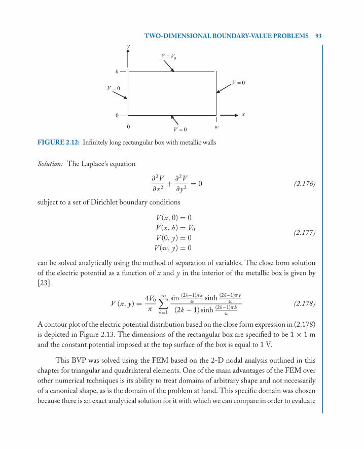
P1: IML/FFX P2: IML
MOBK021-02 MOBK021-Polycarpou.cls April 29, 2006 20:28
TWO-DIMENSIONAL BOUNDARY-VALUE PROBLEMS 93
0 w
h
0 x
y
0V =0V =
0V V=
0V =
FIGURE 2.12: Infinitely long rectangular box with metallic walls
Solution: The Laplace’s equation
∂2V
∂x2+ ∂2V
∂y2= 0 (2.176)
subject to a set of Dirichlet boundary conditions
V (x, 0) = 0
V (x, h) = V0
V (0, y) = 0
V (w, y) = 0
(2.177)
can be solved analytically using the method of separation of variables. The close form solution
of the electric potential as a function of x and y in the interior of the metallic box is given by
[23]
V (x, y) = 4V0
π
∞∑k=1
sin (2k−1)πxw
sinh (2k−1)π yw
(2k − 1) sinh (2k−1)πhw
(2.178)
A contour plot of the electric potential distribution based on the close form expression in (2.178)
is depicted in Figure 2.13. The dimensions of the rectangular box are specified to be 1 × 1 m
and the constant potential imposed at the top surface of the box is equal to 1 V.
This BVP was solved using the FEM based on the 2-D nodal analysis outlined in this
chapter for triangular and quadrilateral elements. One of the main advantages of the FEM over
other numerical techniques is its ability to treat domains of arbitrary shape and not necessarily
of a canonical shape, as is the domain of the problem at hand. This specific domain was chosen
because there is an exact analytical solution for it with which we can compare in order to evaluate
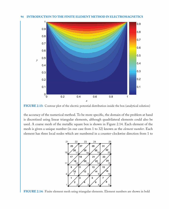
P1: IML/FFX P2: IML
MOBK021-02 MOBK021-Polycarpou.cls April 29, 2006 20:28
94 INTRODUCTION TO THE FINITE ELEMENT METHOD IN ELECTROMAGNETICS
FIGURE 2.13: Contour plot of the electric potential distribution inside the box (analytical solution)
the accuracy of the numerical method. To be more specific, the domain of the problem at hand
is discretized using linear triangular elements, although quadrilateral elements could also be
used. A coarse mesh of the metallic square box is shown in Figure 2.14. Each element of the
mesh is given a unique number (in our case from 1 to 32) known as the element number. Each
element has three local nodes which are numbered in a counter-clockwise direction from 1 to
1 3 5 7
9 11 13 15
6 7 8 10
11 12 13 14 15
16 19 20
21 22 23 24 25
1 2 3 4 52 4 6 8
10 12 14 16
17 19 21 23
18 20 22 24
25 27 29 31
26 28 30 32 1817
9
FIGURE 2.14: Finite element mesh using triangular elements. Element numbers are shown in bold

P1: IML/FFX P2: IML
MOBK021-02 MOBK021-Polycarpou.cls April 29, 2006 20:28
TWO-DIMENSIONAL BOUNDARY-VALUE PROBLEMS 95
3. In addition, each node is given a unique number that is widely referred to as the global node
number. For the particular mesh shown in Figure 2.14, there are 25 global nodes which are
numbered sequentially from 1 to 25. Thus, the global coefficient matrix will have dimensions
25 × 25, whereas the global right-hand-side vector will have dimensions 25 × 1.
The global matrix and right-hand-side vector are formed through the process of assembly,
as outlined in Section 2.6. Now, to construct the element matrices and vectors, which are used
during the assembly of the global matrix and vector, it is important to realize that the Laplace’s
equation in (2.176) is a special case of the generic second-order partial differential equation in
(2.1), i.e.,
∂
∂x
(αx
∂u
∂x
)+ ∂
∂y
(αy
∂u
∂y
)+ βu = g (2.179)
By comparing (2.179) with (2.176), it can be deduced that
u = V
αx = αy = 1
β = 0
g = 0
(2.180)
In addition, for the specific problem at hand, there exist only Dirichlet boundary condi-
tions and no mixed boundary conditions. In other words, there is no boundary �2. Concerning
the Dirichlet boundary conditions, note that three of them are homogeneous whereas one of
them is nonhomogeneous. A 2-D nodal finite element Matlab code, named FEM2DL Box,
was written to solve the Laplace’s equation with the associated Dirichlet boundary conditions.
The code utilizes linear triangular elements. Contour plots of the electric potential in the inte-
rior of the metallic box are depicted in Figures 2.15(a) and 2.15(b) for a coarse and a fine mesh,
respectively. By visually comparing the contour plots in Figures 2.15(a) and 2.15(b) with the
corresponding plot in Figure 2.13, it is observed that a good representation of the exact solution
can be obtained using the FEM provided the discretization of the domain is fine enough. The
accuracy of the numerical solution can be evaluated by computing the error as a function of
mesh size using the L2-norm definition
error =√√√√ 1
Np
Np∑i=1
(ue
i − uni
)2(2.181)
where uei represents the exact analytical solution at a specific grid point, un
i represents the
numerical solution at the same point, and Np represents the total number of points where the
two solutions are evaluated. A plot of the numerical error as a function of discretization size is
illustrated in Figure 2.16. The horizontal axis corresponds to the length of an edge along the x
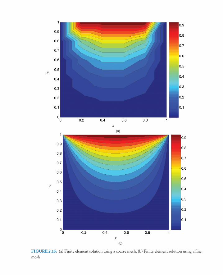
P1: IML/FFX P2: IML
MOBK021-02 MOBK021-Polycarpou.cls April 29, 2006 20:28
(a)
(b)
FIGURE 2.15: (a) Finite element solution using a coarse mesh. (b) Finite element solution using a fine
mesh
96
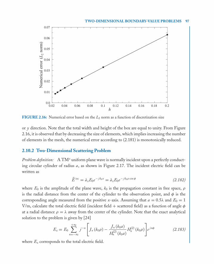
P1: IML/FFX P2: IML
MOBK021-02 MOBK021-Polycarpou.cls April 29, 2006 20:28
TWO-DIMENSIONAL BOUNDARY-VALUE PROBLEMS 97
0.02 0.04 0.06 0.08 0.1 0.12 0.14 0.16 0.18 0.2h
0.0
0.01
0.02
0.03
0.04
0.05
0.06
0.07
Num
eric
aler
ror
(L2
norm
)
FIGURE 2.16: Numerical error based on the L2 norm as a function of discretization size
or y direction. Note that the total width and height of the box are equal to unity. From Figure
2.16, it is observed that by decreasing the size of elements, which implies increasing the number
of elements in the mesh, the numerical error according to (2.181) is monotonically reduced.
2.10.2 Two-Dimensional Scattering Problem
Problem definition: A TMz uniform plane wave is normally incident upon a perfectly conduct-
ing circular cylinder of radius a , as shown in Figure 2.17. The incident electric field can be
written as
�E inc = azE0e− jk0x = azE0e− jk0ρ cos φ (2.182)
where E0 is the amplitude of the plane wave, k0 is the propagation constant in free space, ρ
is the radial distance from the center of the cylinder to the observation point, and φ is the
corresponding angle measured from the positive x-axis. Assuming that a = 0.5λ and E0 = 1
V/m, calculate the total electric field (incident field + scattered field) as a function of angle φ
at a radial distance ρ = λ away from the center of the cylinder. Note that the exact analytical
solution to the problem is given by [24]
Ez = E0
+∞∑n=−∞
j−n
[Jn (k0ρ) − Jn (k0a)
H(2)n (k0a)
H(2)n (k0ρ)
]e jnφ (2.183)
where Ez corresponds to the total electric field.
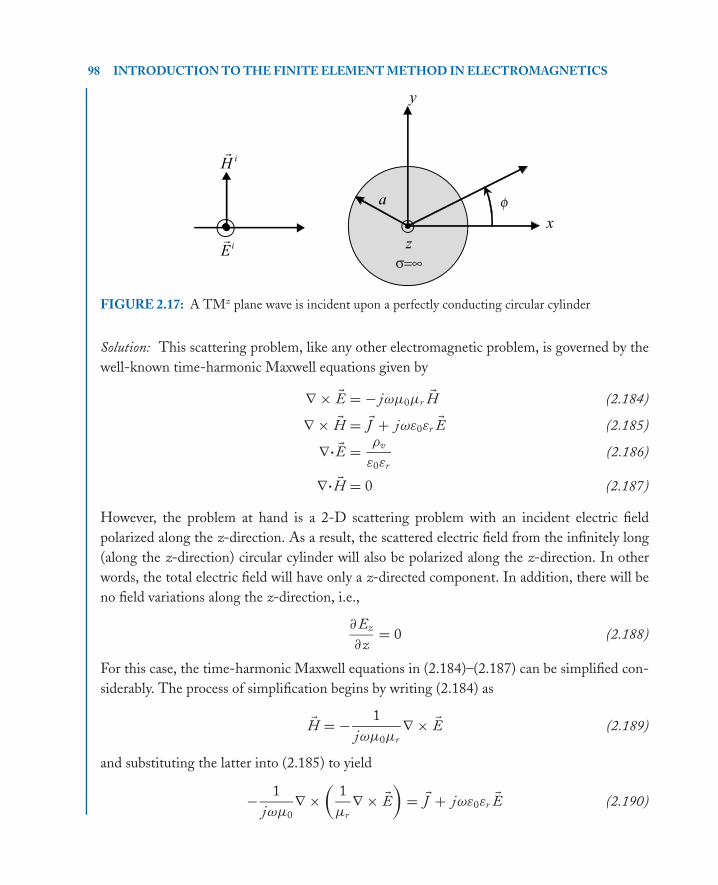
P1: IML/FFX P2: IML
MOBK021-02 MOBK021-Polycarpou.cls April 29, 2006 20:28
98 INTRODUCTION TO THE FINITE ELEMENT METHOD IN ELECTROMAGNETICS
x
y
z
a
iEr
iHr
σ=∞
f
FIGURE 2.17: A TMz plane wave is incident upon a perfectly conducting circular cylinder
Solution: This scattering problem, like any other electromagnetic problem, is governed by the
well-known time-harmonic Maxwell equations given by
∇ × �E = − jωμ0μr�H (2.184)
∇ × �H = �J + jωε0εr�E (2.185)
∇· �E = ρv
ε0εr
(2.186)
∇· �H = 0 (2.187)
However, the problem at hand is a 2-D scattering problem with an incident electric field
polarized along the z-direction. As a result, the scattered electric field from the infinitely long
(along the z-direction) circular cylinder will also be polarized along the z-direction. In other
words, the total electric field will have only a z-directed component. In addition, there will be
no field variations along the z-direction, i.e.,
∂ Ez
∂z= 0 (2.188)
For this case, the time-harmonic Maxwell equations in (2.184)–(2.187) can be simplified con-
siderably. The process of simplification begins by writing (2.184) as
�H = − 1
jωμ0μr
∇ × �E (2.189)
and substituting the latter into (2.185) to yield
− 1
jωμ0
∇ ×(
1
μr
∇ × �E)
= �J + jωε0εr�E (2.190)
P1: IML/FFX P2: IML
MOBK021-02 MOBK021-Polycarpou.cls April 29, 2006 20:28
TWO-DIMENSIONAL BOUNDARY-VALUE PROBLEMS 99
The relative permeability μr cannot be taken out of the curl–curl expression unless it is a
constant. To retain generality, it was decided that the relative permeability of the medium be
treated as a space dependent quantity.
Now, since the total electric field (incident plus scattered) is z-directed, we can write that
∇ ×(
1
μr
∇ × (azEz)
)= − jωμ0 (az Jz) + k2
0εr (azEz) (2.191)
where
k20 = ω2μ0ε0 (2.192)
Using the definition of the curl of a vector in Cartesian coordinates
∇ × �E = ax
(∂ Ez
∂y− ∂ Ey
∂z
)+ a y
(∂ Ex
∂z− ∂ Ez
∂x
)+ az
(∂ Ey
∂x− ∂ Ex
∂y
)(2.193)
and the fact that field variation along the z-direction is zero, see (2.188), the curl–curl expression
in (2.191) can be written as
∇ ×(
1
μr
∇ × (azEz)
)= az
[− ∂
∂x
(1
μr
∂ Ez
∂x
)− ∂
∂y
(1
μr
∂ Ez
∂y
)](2.194)
Substituting (2.194) into (2.191), eliminating the unit vector along the z-direction, and rear-
ranging the terms, we have
∂
∂x
(1
μr
∂ Ez
∂x
)+ ∂
∂y
(1
μr
∂ Ez
∂y
)+ k2
0εr Ez = jωμ0 Jz (2.195)
which is known as the inhomogeneous scalar wave equation. In case we have a source-free region,
as is the problem at hand, the impressed source current Jz must be set to zero, therefore having
∂
∂x
(1
μr
∂ Ez
∂x
)+ ∂
∂y
(1
μr
∂ Ez
∂y
)+ k2
0εr Ez = 0 (2.196)
which is known as the homogeneous scalar wave equation. The latter is the governing partial
differential equation of the scattering problem under consideration.
A finite element formulation was developed early in this chapter to solve the generic
partial differential equation in (2.1). Comparing (2.196) with (2.1), we observe that the former
is a special case of the latter. In other words,
u = Ez
αx = αy = 1
μr
β = k20εr
g = 0
(2.197)
P1: IML/FFX P2: IML
MOBK021-02 MOBK021-Polycarpou.cls April 29, 2006 20:28
100 INTRODUCTION TO THE FINITE ELEMENT METHOD IN ELECTROMAGNETICS
Consequently, the same expressions derived in this chapter for the evaluation of the element
matrices and vectors can be used for the finite element solution of the homogeneous scalar
wave equation in (2.196). As far as boundary conditions are concerned, the total tangential
electric field on perfectly conducting surfaces, denoted by �1, must vanish. In other words, on
the surface of the circular cylinder the z-directed total electric field is zero, i.e.,
Ez = 0 on �1 (2.198)
Furthermore, the domain of the problem is unbounded since this is a scattering problem and,
therefore, the field scattered by the cylinder must continue propagating toward infinity without
disturbance.
The question is how do we simulate numerically this undisturbed wave propagation to
infinity? In an electromagnetic anechoic chamber, absorbing cones are placed on the walls,
ceiling and floor in order to reduce the unwanted reflections by the surroundings. This in
effect simulates outward and undisturbed wave propagation. In the context of the FEM, as
well as other numerical methods such as the finite-difference time-domain (FDTD) method
[25, 26], the numerical domain must be truncated at a certain distance away from the object,
and on the outer boundary of the domain, an ABC [27–31] must be imposed. The purpose of
this ABC, which corresponds to a partial differential equation involving the primary unknown
variable and derivatives of it, is to allow the wave to propagate in the outward direction without
causing any numerical reflections back to the object. Depending on the highest degree of the
derivatives involved in an ABC, there exist different orders such as first-order ABC, second-
order ABC, etc. As the order of the ABC increases, the complexity of it increases as well;
however, the effectiveness of the ABC improves accordingly. Other ways of properly terminating
the unbounded domain of a scattering or radiation problem also exist including the popular
and widely used perfectly matched layer (PML) [32–35], which will not be discussed here. The
advantage of an ABC over the PML is that it does not increase the size of the global matrix
and retains sparsity whereas the PML, although it retains sparsity, it increases the number of
unknowns and worsens the condition number of the matrix system. The main advantages of
PML over ABC include straightforward implementation and improved accuracy.
For the present scattering problem, it was decided that a first-order ABC be used in order
to illustrate the process of imposing such a condition. A second-order ABC can also be used
but, of course, with a bit more complexity involved during its implementation. This will be left
as an exercise to the reader. According to Bayliss et al. [28, 29], a first-order ABC to be imposed
on a circular boundary at a certain distance away from the scatterer is given by
∂ F sca
∂ρ+
(jk0 + 1
2ρ
)F sca = 0 (2.199)

P1: IML/FFX P2: IML
MOBK021-02 MOBK021-Polycarpou.cls April 29, 2006 20:28
TWO-DIMENSIONAL BOUNDARY-VALUE PROBLEMS 101
where F sca denotes the scattered field whether that is electric or magnetic, and ρ is the radial
distance from the center of the circular domain to the outer boundary. The farther away this
circular boundary is placed from the scatterer, the more accurate the finite element solution will
be [29]. A good rule of thumb is to place the first-order ABC at least half a wavelength away
from the outer surface of the scatterer.
Substituting the scattered electric field in (2.199) and realizing that the total electric field
can be written as a sum of the incident and scattered fields,
Ez = E scaz + E inc
z ⇒ E scaz = Ez − E inc
z (2.200)
we can express (2.199) as
∂ Ez
∂ρ+
(jk0 + 1
2ρ
)Ez = ∂ E inc
z
∂ρ+
(jk0 + 1
2ρ
)E inc
z (2.201)
By realizing that the ρ-direction is normal to the outer boundary where the ABC is being
imposed, the first derivative with respect to ρ can be written in a more convenient form given
by
∂ Ez
∂ρ=
(∂ Ez
∂xax + ∂ Ez
∂ya y
)· an (2.202)
where an is the normal unit vector to the outer boundary. Thus, substituting (2.202) into (2.201),
yields(∂ Ez
∂xax + ∂ Ez
∂ya y
)· an +
(jk0 + 1
2ρ
)Ez =
(∂ Einc
z
∂xax + ∂ Einc
z
∂ya y
)· an +
(jk0 + 1
2ρ
)Einc
z
(2.203)
The incident electric field is given, in its general form, by
Eincz = E0e− jk0(x cos φi +y sin φi ) (2.204)
where φi is the incident angle measured with respect to the positive x-axis. Note, however, that
according to the problem definition the incident angle was set to zero, thus
Eincz = E0e− jk0x (2.205)
Substituting (2.205) into the right-hand side of (2.203) and carrying out the derivatives, we
obtain(∂ Ez
∂xax + ∂ Ez
∂ya y
)· an +
(jk0 + 1
2ρ
)Ez = − jk0 Einc
z (ax · an) +(
jk0 + 1
2ρ
)Einc
z
(2.206)
P1: IML/FFX P2: IML
MOBK021-02 MOBK021-Polycarpou.cls April 29, 2006 20:28
102 INTRODUCTION TO THE FINITE ELEMENT METHOD IN ELECTROMAGNETICS
Comparing (2.206) with the mixed boundary condition in (2.6), after setting
αx = αy = 1
μr
= 1 (2.207)
since the outer boundary of the domain (i.e., �2) belongs to free space—it is concluded that
γ = jk0 + 1
2ρ(2.208)
q = − jk0 Eincz (ax · an) +
(jk0 + 1
2ρ
)Einc
z (2.209)
As a result, a first-order ABC on boundary �2 can be imposed through the use of the
mixed boundary condition in (2.6) and the assignment of γ and q according to (2.208) and
(2.209). The process of imposing a mixed boundary condition was explained in detail in Section
2.5. However, in the implementation of the mixed boundary condition in Section 2.5, it was
assumed that both γ and q are constant along �2. As seen, however, from (2.208) and (2.209)
only γ is constant whereas q is a function of space coordinate x. Thus, it has to be taken
into account when evaluating the integral of (2.67). In other words, q cannot be taken out of
the integral as was done in Section 2.5. Specifically, assuming edge 1 → 2 lies on the ABC
boundary, the corresponding entries of element vector pe are given by
pe1 = E0q0�12e− jk0xe
1
(1 − jk0x21 − e− jk0x21
(k0x21)2
)pe
2 = E0q0�12e− jk0xe1
(−1 + ( jk0x21 + 1) e− jk0x21
(k0x21)2
)pe
3 = 0
(2.210)
where
q0 = γ − jk0
(ye
2 − ye1
)�12
(2.211)
If it were edge 3 → 1 lying on the ABC boundary, instead of edge 1 → 2, the entries of
element vector pe would take the following form:
pe1 = E0q0�13e− jk0xe
3
(−1 + ( jk0x13 + 1) e− jk0x13
(k0x13)2
)pe
2 = 0
pe3 = E0q0�13e− jk0xe
3
(1 − jk0x13 − e− jk0x13
(k0x13)2
) (2.212)
where
q0 = γ − jk0
(ye
1 − ye3
)�13
(2.213)
P1: IML/FFX P2: IML
MOBK021-02 MOBK021-Polycarpou.cls April 29, 2006 20:28
TWO-DIMENSIONAL BOUNDARY-VALUE PROBLEMS 103
And at last, if it were edge 2 → 3 lying on the ABC boundary, the entries of element
vector pe would be
pe1 = 0
pe2 = E0q0�23e− jk0xe
2
(1 − jk0x32 − e− jk0x32
(k0x32)2
)pe
3 = E0q0�23e− jk0xe2
(−1 + ( jk0x32 + 1) e− jk0x32
(k0x32)2
) (2.214)
where
q0 = γ − jk0
(ye
3 − ye2
)�23
(2.215)
It is important to reemphasize at this point that the global nodes of each triangle in the mesh
be stored in the connectivity information array in a counter-clockwise direction, otherwise the
above expressions will not be valid.
A 2-D nodal finite element code, named FEM2DL--Cyl, was written in Matlab to
solve the scattering problem described in this section. The major parts of the code include
discretization of the domain using linear triangular elements, generation of proper mesh data,
construction of element matrices and vectors for each element in the domain, assembly of these
element matrices and vectors into the global matrix and right-hand-side vector, imposition of
Dirichlet boundary conditions on the surface of the circular cylinder, and finally solution of the
matrix system to obtain the total electric field at the nodes of the domain. The electric field at
any point in the domain can be evaluated, as outlined in Section 2.9, by using the governing set
of interpolation functions. A relatively coarse mesh of the domain is shown in Figure 2.18. The
radius of the circular conducting cylinder, identified in the figure by the inner circular boundary,
is λ/2 whereas the radius of the ABC boundary, identified in the figure by the outer circular
boundary, is 3λ/2. In other words, the first-order ABC is imposed a distance of one wavelength
away from the outer surface of the object.
Figure 2.19 shows a contour plot of the normalized (to the amplitude of the incident
field) magnitude of the total electric field in the discretized domain. The discretization size was
approximately λ/25. For acceptable results, the discretization size should not be larger than λ/10
whereas the ABC boundary must not be placed closer than a distance of λ/2 from the outer
surface of the object. A comparison between the finite element solution and the exact analytical
solution is shown in Figure 2.20. The evaluation of the field occurs half way between the outer
surface of the conducting cylinder and the ABC boundary. Note that the discretization size is
roughly λ/25, and the ABC boundary is of circular type with radius 3λ/2.

P1: IML/FFX P2: IML
MOBK021-02 MOBK021-Polycarpou.cls April 29, 2006 20:28
104 INTRODUCTION TO THE FINITE ELEMENT METHOD IN ELECTROMAGNETICS
FIGURE 2.18: A coarse triangular mesh of the finite element domain
FIGURE 2.19: Contour plot of the total electric field based on a finite element solution
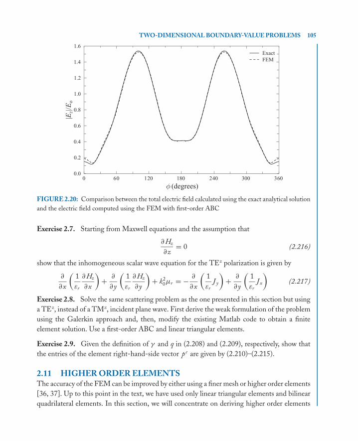
P1: IML/FFX P2: IML
MOBK021-02 MOBK021-Polycarpou.cls April 29, 2006 20:28
TWO-DIMENSIONAL BOUNDARY-VALUE PROBLEMS 105
0 60 120 180 240 300 360
(degrees)
0.0
0.2
0.4
0.6
0.8
1.0
1.2
1.4
1.6
|Ez|
/Eo
Exact
FEM
FIGURE 2.20: Comparison between the total electric field calculated using the exact analytical solution
and the electric field computed using the FEM with first-order ABC
Exercise 2.7. Starting from Maxwell equations and the assumption that
∂ Hz
∂z= 0 (2.216)
show that the inhomogeneous scalar wave equation for the TEz polarization is given by
∂
∂x
(1
εr
∂ Hz
∂x
)+ ∂
∂y
(1
εr
∂ Hz
∂y
)+ k2
0μr = − ∂
∂x
(1
εr
J y
)+ ∂
∂y
(1
εr
J x
)(2.217)
Exercise 2.8. Solve the same scattering problem as the one presented in this section but using
a TEz, instead of a TMz, incident plane wave. First derive the weak formulation of the problem
using the Galerkin approach and, then, modify the existing Matlab code to obtain a finite
element solution. Use a first-order ABC and linear triangular elements.
Exercise 2.9. Given the definition of γ and q in (2.208) and (2.209), respectively, show that
the entries of the element right-hand-side vector pe are given by (2.210)–(2.215).
2.11 HIGHER ORDER ELEMENTSThe accuracy of the FEM can be improved by either using a finer mesh or higher order elements
[36, 37]. Up to this point in the text, we have used only linear triangular elements and bilinear
quadrilateral elements. In this section, we will concentrate on deriving higher order elements
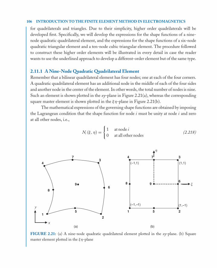
P1: IML/FFX P2: IML
MOBK021-02 MOBK021-Polycarpou.cls April 29, 2006 20:28
106 INTRODUCTION TO THE FINITE ELEMENT METHOD IN ELECTROMAGNETICS
for quadrilaterals and triangles. Due to their simplicity, higher order quadrilaterals will be
developed first. Specifically, we will develop the expressions for the shape functions of a nine-
node quadratic quadrilateral element, and the expressions for the shape functions of a six-node
quadratic triangular element and a ten-node cubic triangular element. The procedure followed
to construct these higher order elements will be illustrated in every detail in case the reader
wants to use the underlined approach to develop a different-order element but of the same type.
2.11.1 A Nine-Node Quadratic Quadrilateral Element
Remember that a bilinear quadrilateral element has four nodes; one at each of the four corners.
A quadratic quadrilateral element has an additional node in the middle of each of the four sides
and another node in the center of the element. In other words, the total number of nodes is nine.
Such an element is shown plotted in the xy-plane in Figure 2.21(a), whereas the corresponding
square master element is shown plotted in the ξη-plane in Figure 2.21(b).
The mathematical expressions of the governing shape functions are obtained by imposing
the Lagrangean condition that the shape function for node i must be unity at node i and zero
at all other nodes, i.e.,
Ni (ξ, η) ={
1 at node i
0 at all other nodes(2.218)
(a) (b)
(–1,–1) (1,–1)
(1,1) (–1,1)
x
y
1 5
2
6
3 7
4
8
9
1 5 2
6
3 7 4
8 9 x
h
FIGURE 2.21: (a) A nine-node quadratic quadrilateral element plotted in the xy-plane. (b) Square
master element plotted in the ξη-plane
P1: IML/FFX P2: IML
MOBK021-02 MOBK021-Polycarpou.cls April 29, 2006 20:28
TWO-DIMENSIONAL BOUNDARY-VALUE PROBLEMS 107
To illustrate the approach used in deriving these shape functions, let us first consider
node 1:
N1 (ξ, η) ={
1 at node 1; i.e., ξ = −1 and η = −1
0 at all other nodes(2.219)
Referring to the square master element in Figure 2.21(b), it is observed that all the nodes,
besides node 1, reside on the horizontal lines
η = 0
η − 1 = 0(2.220)
and the vertical lines
ξ = 0
ξ − 1 = 0(2.221)
Therefore, to impose the condition that N1 be zero at all nodes besides node 1, its expression
must have the form
N1(ξ, η) = c ξη(ξ − 1)(η − 1) (2.222)
Constant c is determined by imposing the second condition which says that N1 be unity at node
1. Doing so, we have
1 = c (−1)(−1)(−2)(−2)
⇒ c = 1
4
(2.223)
Substituting constant c into (2.222), the final expression for N1 is given by
N1(ξ, η) = 1
4ξη(ξ − 1)(η − 1) (2.224)
The same exact procedure can be repeated for the remaining eight nodes to determine
the governing expressions for the corresponding shape functions. These are given below for the
sake of completeness:
N2(ξ, η) = 1
4ξη(ξ + 1)(η − 1) (2.225)
N3(ξ, η) = 1
4ξη(ξ + 1)(η + 1) (2.226)
N4(ξ, η) = 1
4ξη(ξ − 1)(η + 1) (2.227)

P1: IML/FFX P2: IML
MOBK021-02 MOBK021-Polycarpou.cls April 29, 2006 20:28
108 INTRODUCTION TO THE FINITE ELEMENT METHOD IN ELECTROMAGNETICS
N5(ξ, η) = 1
2η(ξ + 1)(ξ − 1)(η − 1) (2.228)
N6(ξ, η) = −1
2ξ (ξ + 1)(η + 1)(η − 1) (2.229)
N7(ξ, η) = −1
2η(ξ + 1)(ξ − 1)(η + 1) (2.230)
N8(ξ, η) = −1
2ξ (ξ − 1)(η + 1)(η − 1) (2.231)
N9(ξ, η) = (ξ + 1)(ξ − 1)(η + 1)(η − 1) (2.232)
Exercise 2.10. Using the same approach illustrated for shape function N1, show that the
remaining shape functions governing a nine-node quadratic quadrilateral element are given by
(2.225)–(2.232).
2.11.2 A Six-Node Quadratic Triangular Element
A quadratic triangular element can be constructed by introducing an additional node at the
midpoint of each of the three edges of a linear triangle. In other words, a quadratic triangle,
shown plotted in the xy-plane in Figure 2.22(a), has a total of six nodes: one at each vertex and
one at the midpoint of each of the three edges. The corresponding master triangular element,
plotted in the ξη-plane, is depicted in Figure 2.22(b).
1
2
3
4
5
6
x
y
1 4 2
5
3
6
0= 2x - 1 = 0
(a) (b)
x
2h - 1 = 0
h = 0
2x + 2h −1= 0 x+h − 1 = 0
FIGURE 2.22: (a) A six-node quadratic triangular element plotted in the xy-plane. (b) Master element
plotted in the ξη-plane
P1: IML/FFX P2: IML
MOBK021-02 MOBK021-Polycarpou.cls April 29, 2006 20:28
TWO-DIMENSIONAL BOUNDARY-VALUE PROBLEMS 109
Assuming isoparametric representation, the primary unknown quantity and the space
coordinates x and y can be expressed according to
u =6∑
i=1
uei Ni
x =6∑
i=1
xei Ni
y =6∑
i=1
yei Ni
(2.233)
where Ni are the Lagrange shape functions defined as
Ni ={
1 at node i
0 at all other nodes(2.234)
For node 1, the corresponding shape function, referring to the master element in Figure
2.22(b), must have the form
N1 = c (2ξ + 2η − 1)(ξ + η − 1) (2.235)
Evaluating (2.235) at node 1 where ξ = 0 and η = 0, constant c is found to be
c = 1 (2.236)
Thus, the final form of N1 is
N1 = (2ξ + 2η − 1)(ξ + η − 1) (2.237)
Similarly,
N2 ={
1 at node 2
0 at all other nodes(2.238)
The second requirement in (2.238) is satisfied provided that the shape function N2 has the form
N2 = c ξ (2ξ − 1) (2.239)
The requirement that N2 = 1 at node 2 must be imposed in order to determine the value of
constant c . Doing so, it is found that
c = 1 (2.240)
Thus, the final expression of N2 is given by
N2 = ξ (2ξ − 1) (2.241)
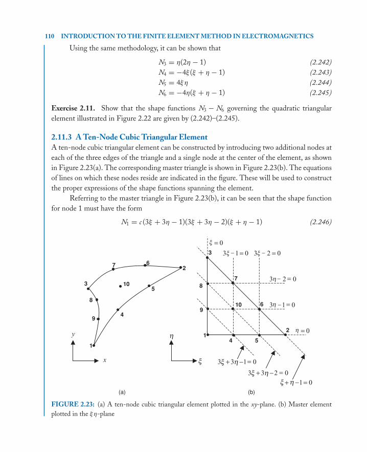
P1: IML/FFX P2: IML
MOBK021-02 MOBK021-Polycarpou.cls April 29, 2006 20:28
110 INTRODUCTION TO THE FINITE ELEMENT METHOD IN ELECTROMAGNETICS
Using the same methodology, it can be shown that
N3 = η(2η − 1) (2.242)
N4 = −4ξ (ξ + η − 1) (2.243)
N5 = 4ξη (2.244)
N6 = −4η(ξ + η − 1) (2.245)
Exercise 2.11. Show that the shape functions N3 − N6 governing the quadratic triangular
element illustrated in Figure 2.22 are given by (2.242)–(2.245).
2.11.3 A Ten-Node Cubic Triangular Element
A ten-node cubic triangular element can be constructed by introducing two additional nodes at
each of the three edges of the triangle and a single node at the center of the element, as shown
in Figure 2.23(a). The corresponding master triangle is shown in Figure 2.23(b). The equations
of lines on which these nodes reside are indicated in the figure. These will be used to construct
the proper expressions of the shape functions spanning the element.
Referring to the master triangle in Figure 2.23(b), it can be seen that the shape function
for node 1 must have the form
N1 = c (3ξ + 3η − 1)(3ξ + 3η − 2)(ξ + η − 1) (2.246)
1
2
3
4
5
6 7
8
9
10
x
y 12
3
4 5
6
78
910
3 1 0= 3 2 0=
=
=
3 3 1 0+
3 1 0
0=
0=
0
=
=−
)(a) (b
x
x x- -
h -
h
h
-
3 2
+
x x h3 3 2 0+ =−
−x h
x h
h
1 0
FIGURE 2.23: (a) A ten-node cubic triangular element plotted in the xy-plane. (b) Master element
plotted in the ξη-plane
P1: IML/FFX P2: IML
MOBK021-02 MOBK021-Polycarpou.cls April 29, 2006 20:28
TWO-DIMENSIONAL BOUNDARY-VALUE PROBLEMS 111
All nodes, besides node 1, reside on the three inclined lines whose equations are indicated in the
figure. The corresponding shape function for node 1 must be zero at all those nodes and that is
why the proper form of N1 is given by (2.246). To determine constant c , it is necessary to impose
the requirement that the shape function be unity at node 1. Doing so, it can be shown that
c = −1
2(2.247)
Thus, the shape function for node 1 is given by
N1 = −1
2(3ξ + 3η − 1)(3ξ + 3η − 2)(ξ + η − 1) (2.248)
In a similar way, we can derive the remaining shape functions. For the sake of completeness,
these are given below:
N2 = 1
2ξ (3ξ − 1)(3ξ − 2) (2.249)
N3 = 1
2η(3η − 1)(3η − 2) (2.250)
N4 = 9
2ξ (3ξ + 3η − 2)(ξ + η − 1) (2.251)
N5 = −9
2ξ (3ξ − 1)(ξ + η − 1) (2.252)
N6 = 9
2ξη(3ξ − 1) (2.253)
N7 = −9
2ξη(3ξ − 2) (2.254)
N8 = −9
2η(3η − 1)(ξ + η − 1) (2.255)
N9 = 9
2η(3ξ + 3η − 2)(ξ + η − 1) (2.256)
N10 = −27ξη(ξ + η − 1) (2.257)
Exercise 2.12. Using the same approach illustrated for the derivation of N1, show that the shape
functions N2 − N10 for the cubic triangular element in Figure 2.23 are given by (2.249)–(2.257).
2.12 SOFTWARETwo Matlab codes were written to solve the two application problems discussed in this chapter.
The first code (FEM2DL--Box), which uses linear triangular elements, was written to solve
the electrostatic BVP, presented in this chapter, for a rectangular domain. Three of the walls
are set to a zero potential whereas the top horizontal wall was set to a nonzero potential. The
user, among other parameters, has the freedom to change the density of the mesh. The code
computes the primary unknown quantity, which is the electrostatic potential, and the numerical
P1: IML/FFX P2: IML
MOBK021-02 MOBK021-Polycarpou.cls April 29, 2006 20:28
112 INTRODUCTION TO THE FINITE ELEMENT METHOD IN ELECTROMAGNETICS
error based on the L2 norm. The second code (FEM2DL--Cyl), which also uses linear elements,
was written to solve the scattering problem, presented in this chapter, for a conducting circular
cylinder. The program generates a triangular mesh, based on the user’s choice of discretization
size, and computes the total field everywhere in the domain. Note that the total field is a
superposition of the scattered field and the incident field. A TMz polarization was considered.
The reader is encouraged to execute these codes in Matlab, modify certain parameters
such as discretization size, object dimensions, distance to the ABC, etc., and visualize the results.
Whoever is interested can even try to slightly modify these Matlab codes to solve other types of
electromagnetic problems. Both Matlab codes can be downloaded from the publisher’s URL:
www.morganclaypool.com/page/polycarpou.
References
[1] J. C. Nedelec, “A new family of mixed finite elements in R3,” Numer. Methods, vol. 30,
pp. 57–81, 1986.
[2] M. L. Barton and Z. J. Cendes, “New vector finite elements for three-dimensional
magnetic field computation,” J. Appl. Phys., vol. 61, pp. 3919–3921, 1987.
doi:10.1063/1.338584
[3] Z. J. Cendes, “Vector finite elements for electromagnetic field computations,” IEEE
Trans. Magn., vol. MAG-27, no. 5, pp. 3958–3966, Sept. 1991. doi:10.1109/20.104970
[4] J. P. Webb, “Edge elements and what they can do for you,” IEEE Trans. Magn.,
vol. MAG-29, pp. 1460–1465, Mar. 1993. doi:10.1109/20.250678
[5] G. Mur, “The finite-element modeling of three-dimensional electromagnetic fields using
edge and nodal elements,” IEEE Trans. Antennas Propag., vol. 41, no. 7, pp. 948–953,
July 1993. doi:10.1109/8.237627
[6] H. Anton, I. Bivens, and S. Davis, Calculaus, 7th ed. New York: Wiley, 2002, pp. 1075–
1090.
[7] O. C. Zienkiewicz and R. L. Taylor, The Finite Element Method, 4th ed., vol. 1: Basic
Formulation of Linear Problems. New York: McGraw-Hill, 1989.
[8] D. Zwillinger, Handbook of Integration. Boston: Jones and Barlett, 1992.
[9] E. W. Cheney and D. R. Kincaid, Numerical Mathematics and Computing, 5th ed.
Monterey: Brooks Cole, 2003.
[10] M. Abramowitz and I. A. Stegun, Handbook of Mathematical Functions. New York: Dover
Publications, 1972.
[11] G. R. Cowper, “Gaussian quadrature formulas for triangles,” Int. J. Numer. Methods Eng.,
vol. 7, pp. 405–408, 1973. doi:10.1002/nme.1620070316
P1: IML/FFX P2: IML
MOBK021-02 MOBK021-Polycarpou.cls April 29, 2006 20:28
TWO-DIMENSIONAL BOUNDARY-VALUE PROBLEMS 113
[12] R. S. Varga, Matrix Iterative Analysis, Prentice-Hall, Englewood Cliffs, New Jersey, 1962.
[13] D. M. Young, Iterative Solution of Large Linear Systems. New York: Dover Publications,
2003.
[14] Y. Saads, Iterative Methods for Sparse Linear Systems. Boston: PWS Publishing, 1996.
[15] A. M. Bruaset, A Survey of Preconditioned Iterative Methods. London, UK: Chapman &
Hall, 1995.
[16] A. Chatterjee, J. M. Jin, and J. L. Volakis, “Edge-based finite elements and vector ABC’s
applied to 3-D scattering,” IEEE Trans. Antennas Propag., vol. 41, no. 2, pp. 221–226,
Feb. 1993. doi:10.1109/8.214614
[17] J. M. Jin and J. L. Volakis, “A hybrid finite element method for scattering and radiation by
microstrip patch antennas and arrays residing in a cavity,” IEEE Trans. Antennas Propag.,
vol. 39, no. 11, pp. 1598–1604, Nov. 1991. doi:10.1109/8.102775
[18] A. C. Polycarpou, C. A. Balanis, J. T. Aberle, and C. Birtcher, “Radiation and scattering
from ferrite-tuned cavity-backed slot antennas: Theory and experiment,” IEEE Trans.
Antennas Propag., vol. 46, no. 9, pp. 1297–1306, 1998. doi:10.1109/8.719973
[19] D. T. McGrath and V. P. Pyati, “Phased array antenna analysis with the hybrid finite
element method,” IEEE Trans. Antennas Propag., vol. 42, no. 12, pp. 1625–1630, Dec.
1994. doi:10.1109/8.362811
[20] A. Chatterjee, J. M. Jin, and J. L. Volakis, “Computation of cavity resonances using
edge-based finite elements,” IEEE Trans. Microw. Theory Tech., vol. MTT-40, pp. 2106–
2108, Nov. 1992. doi:10.1109/22.168771
[21] J. M. Jin and V. V. Liepa, “Application of hybrid finite element method to electromag-
netic scattering from coated cylinders,” IEEE Trans. Antennas Propag., vol. 36, no. 1,
pp. 50–54, Jan. 1988. doi:10.1109/8.1074
[22] D.-H. Han, A. C. Polycarpou, and C. A. Balanis, “Hybrid analysis of reflector antennas
including higher-order interactions and blockage effects,” IEEE Trans. Antennas Propag.,
vol. 50, no. 11, pp. 1514–1524, 2002. doi:10.1109/TAP.2002.803952
[23] M. N. O. Sadiku, Numerical Techniques in Electromagnetics, 2nd ed. Boca Raton: CRC
Press, 2001.
[24] C. A. Balanis, Advanced Engineering Electromagnetics. New York: Wiley, 1989.
[25] A. Taflove and S. C. Hagness, Computational Electrodynamics: The Finite-Difference Time
Domain Method, 2nd ed. Boston: Artech House, 2000.
[26] K. S. Kunz and R. J. Luebbers, The Finite Difference Time Domain Method for Electro-
magnetics. Boca Ratorn: CRC Press, 1993.
[27] B. Engquist and A. Majda, “Absorbing boundary conditions for the numerical simulation
of waves,” Math. Comput., vol. 31, pp. 329–351, 1977.

P1: IML/FFX P2: IML
MOBK021-02 MOBK021-Polycarpou.cls April 29, 2006 20:28
114 INTRODUCTION TO THE FINITE ELEMENT METHOD IN ELECTROMAGNETICS
[28] A. Bayliss and E. Turkel, “Radiation boundary conditions for wave-like equations,” Com-
mun. Pure Appl. Math., vol. 33, pp. 707–725, 1980.
[29] A. Bayliss, M. Gunzburger, and E. Turkel, “Boundary conditions for the numerical
solution of elliptic equations in exterior regions,” SIAM J. Appl. Math., vol. 42, pp. 430–
451, 1982. doi:10.1137/0142032
[30] A. F. Peterson, “Absorbing boundary conditions for the vector wave equation,” Microw.
Opt. Technol. Lett., vol. 1, pp. 62–64, 1988.
[31] J. P. Webb and V. N. Kanellopoulos, “Absorbing boundary conditions for the finite
element solution of the vector wave equation,” Microw. Opt. Technol. Lett., vol. 2,
pp. 370–372, 1989.
[32] J. P. Berenger, “A perfectly matched layer for the absorption of electromagnetic waves,”
J. Comput. Phys., vol. 114, no. 2, pp. 185–200, Oct. 1994. doi:10.1006/jcph.1994.1159
[33] Z. S. Sacks, D. M. Kingsland, R. Lee, and J.-F. Lee, “A perfectly matched anisotropic
absorber for use as an absorbing boundary condition,” IEEE Trans. Antennas Propag., vol.
43, no. 12, pp. 1460–1463, 1995. doi:10.1109/8.477075
[34] U. Pekel and R. Mittra, “A finite element method frequency domain application of
the perfectly matched layer (PML) concept,” Microw. Opt. Technol. Lett., vol. 9, no. 3,
pp. 117–122, June 1995.
[35] A. C. Polycarpou, M. R. Lyons, and C. A. Balanis, “A two-dimensional finite-element
formulation of the perfectly matched layer,” IEEE Microw. Guided Wave Lett., vol. 8,
pp. 30–32, Jan. 1997.
[36] P. Silvester, “High-order polynomial triangular finite elements for potential problems,”
Int. J. Eng. Sci., vol. 7, pp. 849–861, 1969. doi:10.1016/0020-7225(69)90065-2
[37] P. Silvester, “A general high-order finite-element waveguide analysis program,”
IEEE Trans. Microw. Theory Tech., vol. MTT-17, pp. 204–210, Apr. 1969.
doi:10.1109/TMTT.1969.1126932

P1: IML/FFX P2: IML
MOBK021-02 MOBK021-Polycarpou.cls April 29, 2006 20:28
115
Author Biographies
Anastasis C. Polycarpou received the B.S. (with summa cum laude), M.S., and Ph.D. degrees
in Electrical Engineering from Arizona State University in 1992, 1994, and 1998, respectively.
During his graduate studies, he was with the Telecommunications Research Center (TRC) of
ASU where he worked on various research projects sponsored by government organizations
and private companies such as the US Navy, US Army, Boeing, Sikorsky, and a few more. In
the summer of 1998, he joined the Department of Electrical Engineering of ASU as an Asso-
ciate Research Faculty where he performed research on a variety of subjects in the broad area
of electromagnetics. While being at ASU, he worked on the development and enhancement
of numerical methods, in particular the Finite Element Method (FEM) and the Method of
Moments (MoM), for the analysis of complex electromagnetic problems such as microwave
circuits, interconnects and electronic packaging, cavity-backed slot antennas in the pres-
ence of magnetized ferrites, and helicopter electromagnetics. He wrote a multipurpose three-
dimensional finite element code using edge elements to solve geometrically complex scattering
and radiation problems. The code utilizes advanced iterative techniques in linear algebra for the
solution of extremely large indefinite matrix systems.
Dr. Polycarpou has published more than 40 journals and conference proceedings and two
chapters in books. He is currently an Associate Professor at Intercollege in Cyprus. His research
areas of interest include numerical methods in electromagnetics and specifically the Finite
Element Method and the Method of Moments, antenna analysis and design, electromagnetic
theory, and ferrite materials.

P1: IML/FFX P2: IML
MOBK021-02 MOBK021-Polycarpou.cls April 29, 2006 20:28
116