Identifying differences in the rules of interaction betweenindividuals in moving animal groups

Timothy. M. Schaerf1,†

James E. Herbert-Read2,∗,†

Mary R. Myerscough3

David J. T. Sumpter2

Ashley J. W. Ward1

1. Animal Behaviour Lab, School of Biological Sciences, University of Sydney, Sydney, 2006,Australia;2. Department of Mathematics, Uppsala University, Uppsala, 75106, Sweden;3. School of Mathematics and Statistics, University of Sydney, Sydney, 2006, Australia.∗ Corresponding author; e-mail: james.herbert.read@gmail.com.† These authors contributed equally to this study.

Keywords: Collective motion, Leadership, Social Responsiveness, Gambusia holbrooki.

Manuscript type: Article.

1

arX

iv:1

601.

0820

2v1

[q-

bio.

QM

] 2

8 Ja

n 20

16

Abstract

Collective movement can be achieved whenindividuals respond to the local movementsand positions of their neighbours. Someindividuals may disproportionately influencegroup movement if they occupy particularspatial positions in the group, for example,positions at the front of the group. We asked,therefore, what led individuals in movingpairs of fish (Gambusia holbrooki) to occupya position in front of their partner? Individu-als adjusted their speed and direction differ-ently in response to their partner’s position,resulting in individuals occupying differentpositions in the group. Individuals that werefound most often at the front of the pair hadgreater mean changes in speed than their part-ner, and were less likely to turn towards theirpartner, compared to those individuals mostoften found at the back of the pair. The pairmoved faster when led by the individual thatwas usually at the front. Our results high-light how differences in the social respon-siveness between individuals can give rise toleadership in free moving groups. They alsodemonstrate how the movement characteris-tics of groups depend on the spatial config-uration of individuals within them.

Introduction

Collective motion is often driven through thelocal interactions between individuals in a self-organising process (Couzin et al. 2005, 2002).By responding to the movements and po-sitions of their neighbours, individuals cantransfer information about detected threats ormove together towards target locations (Couzinet al. 2011; Herbert-Read et al. 2015; Sumpter2010). But information does not always prop-agate evenly across groups (Rosenthal et al.2015). When individuals in bird flocks or fishschools travel in the same direction, individu-als positioned at the front of groups are more

likely to initiate changes in the direction ofothers, since individuals cannot observe themovements of those directly behind themselves(Herbert-Read et al. 2011; Nagy et al. 2010).If some individuals within a group occupythese front positions more than others, thenthese individuals can disproportionately influ-ence group motion (Couzin et al. 2011; Reebs2000). In effect, minorities of individuals canguide entire groups (Couzin et al. 2005).

There is evidence that individuals consis-tently occupy different positions within mov-ing groups. Phenotypic characteristics suchas body size can determine where individu-als are located in groups, with larger individu-als sometimes occupying positions at the frontof groups (Pitcher et al. 1982). Differences be-tween individuals’ movements may also lead todifferential spatial positions, with faster mov-ing individuals migrating towards front posi-tions (Couzin et al. 2002; Pettit et al. 2013).However, some individuals occupy positionsin groups that do not seem to be related totheir body size or other phenotypic differences.Burns et al. (2012), for example, found that in-dividual mosquitofish (Gambusia holbrooki) oc-cupied consistent positions within groups, andthis was not related to their sex, body size,or dominance (Burns et al. 2012). Similarly,dominance cannot explain the differential spa-tial positioning of individuals in homing pi-geon flocks (Columbia livia) (Nagy et al. 2013).In these cases, what differences between indi-viduals determine where individuals positionthemselves in groups?

Other factors that are more transient withinan individual may explain the differential po-sitioning behaviour of individuals in groups.In some cases, individuals that are more in-formed about their environment than othergroup members may occupy positions at thefront of groups (Reebs 2001) (but see; Flacket al. 2013). Nutritional state may also affectwhere an individual positions itself in a group,with hungry individuals often being found at

2

the front of groups (Krause et al. 2000). In thesecases, and in the absence of energetic or pheno-typic constraints on movement, it is ultimatelyhow an individual interacts with its neighboursthat leads it to occupy different spatial posi-tions. Information and satiation level influencethe likelihood that an individual will follow an-other conspecific’s movements (King et al. 2011;Leblond and Reebs 2006; Nakayama et al. 2012).If an individual ignores the movements of oth-ers more than others ignore it, then passiveself assortment may move this individual to thefront of groups (Couzin et al. 2005). How anindividual interacts with its neighbours, and inparticular, whether some individuals are more‘socially responsive’ to the movements of oth-ers, therefore, is likely to result in differentialspatial positioning in groups and affect whofollows whom (Harcourt et al. 2009).

How can we measure the responsiveness ofindividuals to each others’ movements? Re-searchers have previously used averaging pro-cedures to determine the general ‘rules’ that in-dividuals in groups use to react to their neigh-bours when on the move (Gautrais et al. 2012;Herbert-Read et al. 2011; Katz et al. 2011; Luke-man et al. 2010). Attraction and repulsion rules,largely governed by changes in speed, appearimportant determinants of how individuals re-spond to their neighbours’ locations and move-ments (Herbert-Read et al. 2011; Katz et al.2011). Alternatively, these rules may be drivenby individuals preferring to occupy particularspatial positions with respect to the locationsof other group members (Perna et al. 2014).The variation in these rules between individ-uals, however, has not been explored exper-imentally, although models of collective mo-tion show that differences between individu-als’ movements and interactions can influencegroup dynamics (Couzin et al. 2005; Romey1996).

We tested whether individuals differed inhow they responded to their partner’s locationand movements in pairs of mosquitofish (Gam-

busia holbrooki) during their exploration of anunfamiliar arena. We first asked whether an in-dividual’s position in the group was related totheir relative size, movement profile (for exam-ple, their average speed) or information aboutthe environment, and then determined whetherdifferences in the social interactions between in-dividuals could lead to individuals occupyingdifferent positions within groups.

Methods

Experiments

Female mosquitofish (n = 80) (Gambusia hol-brooki) were collected using hand-nets fromLake Northam, Sydney, NSW, (33◦53′07′′ S;151◦11′35′′ E). Fish were held in 170 l aquariaand were fed flake food ad libitum. Fish werekept for at least 3 weeks prior to experimenta-tion. A square experimental arena (1.5 m x 1.5m x 0.2 m) was constructed of opaque whiteperspex and filled to a depth of 7 cm. In twocorners of the arena, diagonally opposite oneanother, we placed an opaque white holdingtube (10 cm diameter). For each trial, we se-lected two fish of similar size (approximately1.5 - 2.5 cm) and placed one in each of the hold-ing tubes. To test if a fish’s experience withthe environment subsequently led this individ-ual to occupy positions at the front (or back) ofthe group, following an acclimation period of5 minutes, we either released one (n = 20 tri-als), or both fish (n = 20 trials) into the arena.If we had only released one fish into the arena,we allowed this fish to explore the arena for5 minutes before we released the second fish.In one of the two treatments, therefore, onefish had explored the environment for longerthan the other. We filmed the trials using aBasler avA1600-65kc camera and recorded us-ing StreamPix (version 5) at 40 fps. Fish werefilmed for 6 minutes when both fish had beenreleased into the arena. These films were sub-sequently converted using VirtualDub (version

3

1.9.11) and the fish were tracked using Ctrax(version 0.5.4), (Branson et al. 2009). Any ambi-guities in fish identities or other elements of thetracked data were resolved using Ctrax’s fixer-rors GUI. In addition to time series of each fish’s(x, y) coordinates, we extracted measurementsrelated to the body length of each fish.

Analysis

We smoothed the x and y components of eachfish’s track using a Savitzky-Golay filter (im-plemented through MATLAB’s intrinsic smoothfunction with span 5 and degree 2) prior to alldiagnostic calculations. We only analysed basicindividual characteristics of each fish’s motion,positioning behaviour and directional correla-tion when fish were less than or equal to 100mm apart. This is because we wanted to en-sure we analysed sequences when the pair wasinteracting, and not when individuals were ex-ploring the arena independently. 58.49% of ourtrajectory data satisfied this condition. Further,our analysis of interactions between individu-als was restricted to cases where the relativedisplacement between the fish was less than orequal to 100 mm in both the x or y direction.

Predictors of positioning behaviour inpairs

We first determined which individual in thepair was more often in front of the other (rel-ative to the heading of group motion) over theentire trial. We defined individuals that weremore often observed at the front of the group‘front fish’, and individuals that were more of-ten observed at the back of the group ‘back fish’(see online appendix A for the proportion oftime these individuals occupied different posi-tions).

We then determined the average directionalcorrelation between the two fish as a functionof a delay time to examine the relative influ-ence that fish had on the direction of motion oftheir partner when they were either at the front

or back of the pair (Katz et al. 2011; Nagy et al.2010). We calculated each fish’s speed, mag-nitude of acceleration, change in speed overtime and turning speed for all frames when fishwere less than or equal to 100 mm apart. Wedetermined the mean, standard deviation, me-dian, inter-quartile range and maximum valueof each of these variables for front fish and backfish separately (details of all the above calcula-tions are provided in online appendix A.)

We asked which of the above movement pa-rameters or body size was greater (or less) forfront or back fish. To do this, we treated allthe summary statistics as paired data (front fishversus back fish) and calculated the differencein parameter values between front and backfish. We applied a Shaprio-Wilk test to deter-mine if these differences were likely to havebeen drawn from a normal distribution Shapiroand Wilk 1965. If the data was normally dis-tributed, we then performed a paired t-test todetermine if the mean of the differences dif-fered from zero. If the set of differences wasnot normally distributed, we performed a two-sided Wilcoxon paired-sample test (via MAT-LAB’s intrinsic signrank function) to determineif the median difference in parameters differedfrom zero (see for example, Zar 1996). To ac-count for the number of summary statistics thatwe compared (21 in total), we sorted the re-sults of all statistical tests in ascending orderof p-value, and adjusted the significance level,αsig, for these tests according to the Holm-Bonferroni method (Holm 1979).

Characteristics of individuals’ interac-tions

After application of a Holm-Bonferroni correc-tion the only parameter that differed betweenfish that spent the greatest proportion of timeat the front of their pair and their partner wasmean change in speed over time – a parame-ter intrinsically linked with how an animal in-teracts with its neighbours (Herbert-Read et al.

4

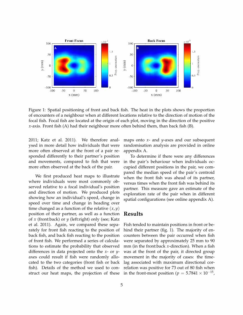
Figure 1: Spatial positioning of front and back fish. The heat in the plots shows the proportionof encounters of a neighbour when at different locations relative to the direction of motion of thefocal fish. Focal fish are located at the origin of each plot, moving in the direction of the positivex-axis. Front fish (A) had their neighbour more often behind them, than back fish (B).

2011; Katz et al. 2011). We therefore anal-ysed in more detail how individuals that weremore often observed at the front of a pair re-sponded differently to their partner’s positionand movements, compared to fish that weremore often observed at the back of the pair.

We first produced heat maps to illustratewhere individuals were most commonly ob-served relative to a focal individual’s positionand direction of motion. We produced plotsshowing how an individual’s speed, change inspeed over time and change in heading overtime changed as a function of the relative (x, y)position of their partner, as well as a functionof x (front:back) or y (left:right) only (see; Katzet al. 2011). Again, we compared these sepa-rately for front fish reacting to the position ofback fish, and back fish reacting to the positionof front fish. We performed a series of calcula-tions to estimate the probability that observeddifferences in data projected onto the x- or y-axes could result if fish were randomly allo-cated to the two categories (front fish or backfish). Details of the method we used to con-struct our heat maps, the projection of these

maps onto x- and y-axes and our subsequentrandomisation analysis are provided in onlineappendix A.

To determine if there were any differencesin the pair’s behaviour when individuals oc-cupied different positions in the pair, we com-pared the median speed of the pair’s centroidwhen the front fish was ahead of its partner,versus times when the front fish was behind itspartner. This measure gave an estimate of theexploration rate of the pair when in differentspatial configurations (see online appendix A).

Results

Fish tended to maintain positions in front or be-hind their partner (fig. 1). The majority of en-counters between the pair occurred when fishwere separated by approximately 25 mm to 90mm (in the front:back x-direction). When a fishwas at the front of the pair, it directed groupmovement in the majority of cases: the time-lag associated with maximum directional cor-relation was positive for 73 out of 80 fish whenin the front-most position (p = 5.7841× 10−15,

5

Figure 2: A The mean speed, B mean change in speed over time, C mean change in angle ofmotion over time of front fish (solid red curve) and back fish (solid blue curve) as a functionof the relative x-coordinate of their partner (A & B) or right-left position (C). Dashed curvesare plotted one standard error above and below all means in each panel. Combined, the meanchange in speed over time (B) and the mean change in angle of motion over time (C) describehow an individual adjusts its velocity as a function of relative partner location. Grey regions inall plots highlight where our randomisation procedure indicated that the sign and magnitude ofthe difference between the front fish curves and back fish curves was unlikely to occur if fish hadrandomly been allocated to the sets of front or back fish.

two-tailed binomial test). Individuals led theirpartner, therefore, when at the front of thegroup. The proportion of frames that the frontfish was found at the front of the group rangedwidely from 0.5004 to 0.9643 (see Tables A1 andA2 and fig. A1 in online appendix A).

Fish that had an additional 5 minutes toexplore the arena were not significantly asso-ciated with being the front fish (p = 0.4119,N = 20, n = 9, two-tailed binomial test). Af-ter application of the Holm-Bonferroni correc-tion, the only difference in movement parame-ters between front fish and back fish was themean change in speed over time; front fishhad greater mean changes speed over time thanback fish (see Table A5 in online appendix A fordetails of statistical tests applied to movementparameters and body length).

We then tested whether the movements offront fish or back fish differed in response totheir partner’s position. Speeds of both thefront fish and the back fish were lowest whentheir partner was close to them (x = 0). The

average speeds adopted by front fish were ap-proximately symmetric about x = 0 (fig. 2 A);front fish tended to travel at a similar speedregardless of whether their partner was at thesame distance in front or behind them (for ex-ample, compare the red curve speeds whenx = 50 mm with x = −50 mm in fig. 2 A).In contrast, there was more pronounced asym-metry in the speeds of back fish as a functionof their neighbour’s position. Back fish tendedto adopt lower speeds when their partner waslocated behind them, and higher speeds whentheir partner was located in front of them (fig. 2A). The differences in the speeds adopted byfront or back fish when their partner was be-hind them (x < −25 mm) were unlikely to oc-cur as a result of randomly allocating fish tocategories of front fish or back fish (see fig. A16E).

Fish also adjusted their speed dependingon their partner’s position. The instantaneouschanges in speed over time as a function oftheir partner’s position were qualitatively sim-

6

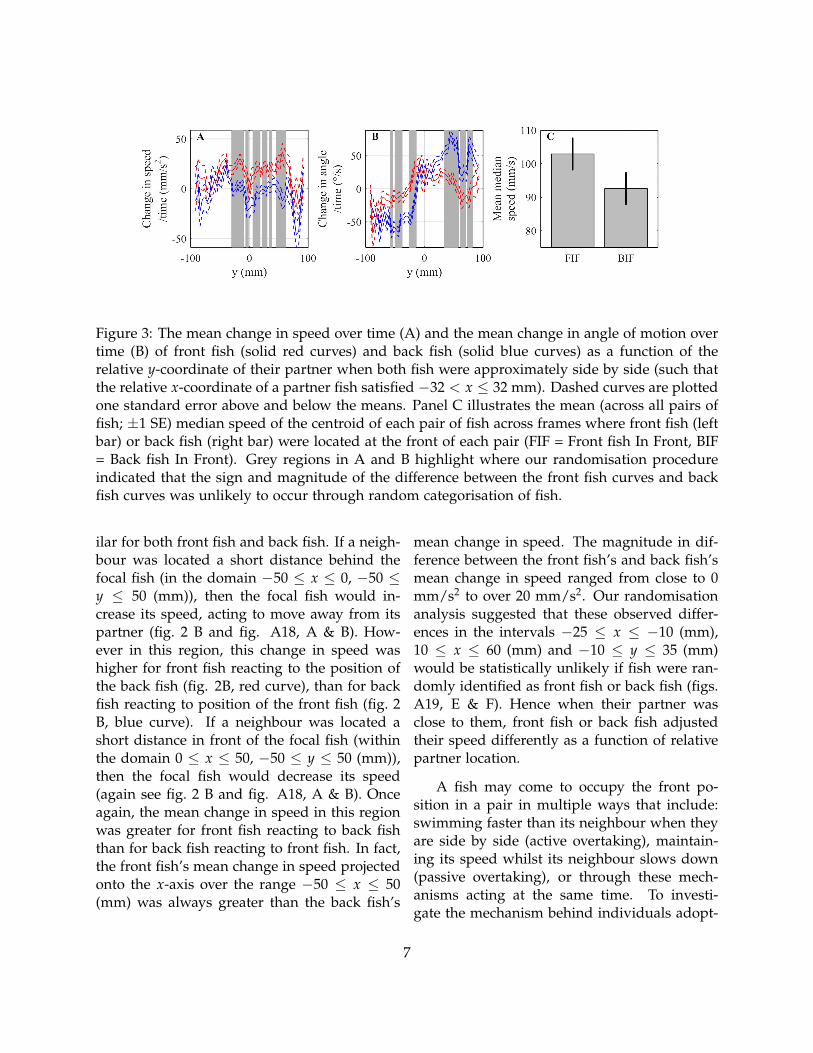
Figure 3: The mean change in speed over time (A) and the mean change in angle of motion overtime (B) of front fish (solid red curves) and back fish (solid blue curves) as a function of therelative y-coordinate of their partner when both fish were approximately side by side (such thatthe relative x-coordinate of a partner fish satisfied −32 < x ≤ 32 mm). Dashed curves are plottedone standard error above and below the means. Panel C illustrates the mean (across all pairs offish; ±1 SE) median speed of the centroid of each pair of fish across frames where front fish (leftbar) or back fish (right bar) were located at the front of each pair (FIF = Front fish In Front, BIF= Back fish In Front). Grey regions in A and B highlight where our randomisation procedureindicated that the sign and magnitude of the difference between the front fish curves and backfish curves was unlikely to occur through random categorisation of fish.

ilar for both front fish and back fish. If a neigh-bour was located a short distance behind thefocal fish (in the domain −50 ≤ x ≤ 0, −50 ≤y ≤ 50 (mm)), then the focal fish would in-crease its speed, acting to move away from itspartner (fig. 2 B and fig. A18, A & B). How-ever in this region, this change in speed washigher for front fish reacting to the position ofthe back fish (fig. 2B, red curve), than for backfish reacting to position of the front fish (fig. 2B, blue curve). If a neighbour was located ashort distance in front of the focal fish (withinthe domain 0 ≤ x ≤ 50, −50 ≤ y ≤ 50 (mm)),then the focal fish would decrease its speed(again see fig. 2 B and fig. A18, A & B). Onceagain, the mean change in speed in this regionwas greater for front fish reacting to back fishthan for back fish reacting to front fish. In fact,the front fish’s mean change in speed projectedonto the x-axis over the range −50 ≤ x ≤ 50(mm) was always greater than the back fish’s

mean change in speed. The magnitude in dif-ference between the front fish’s and back fish’smean change in speed ranged from close to 0mm/s2 to over 20 mm/s2. Our randomisationanalysis suggested that these observed differ-ences in the intervals −25 ≤ x ≤ −10 (mm),10 ≤ x ≤ 60 (mm) and −10 ≤ y ≤ 35 (mm)would be statistically unlikely if fish were ran-domly identified as front fish or back fish (figs.A19, E & F). Hence when their partner wasclose to them, front fish or back fish adjustedtheir speed differently as a function of relativepartner location.

A fish may come to occupy the front po-sition in a pair in multiple ways that include:swimming faster than its neighbour when theyare side by side (active overtaking), maintain-ing its speed whilst its neighbour slows down(passive overtaking), or through these mech-anisms acting at the same time. To investi-gate the mechanism behind individuals adopt-

7

ing front positions, we compared each fish’schange in speed over time (projected onto they-axis) when both fish were approximately sideby side (where −32 < x ≤ 32 (mm), that is,where the difference in the x-coordinates of thefish differed by up to a little over one bodylength). Front fish generally had a greater meanchange in speed over time than their partner inthis region (fig. 3 A). Further, front fish tendedto exhibit positive changes in speed, whereastheir partners exhibited changes in speed thatwere closer to zero, and in some instances neg-ative (fig. 3 A), especially over the approximaterange −25 ≤ y ≤ 60 mm. These results suggestthat front fish tended to accelerate to either takeor maintain the frontmost position (active over-taking), whereas back fish tended to continue attheir current speed or even reduce their speedwhen the front position was in contest, in effect,giving way to their partner. Our randomisa-tion analysis suggested that the sign and mag-nitude of the difference in leader and followerchanges in speed over time in fig. 3 A were un-likely to occur if fish were randomly allocatedto front fish or back fish categories for datain smaller regions contained within the range−30 ≤ y ≤ 60 mm (see fig. A22, E).

In general, both front fish and back fish ex-hibited a tendency to turn towards their part-ners, with fish turning anti-clockwise (charac-terised by positive changes in angle of motion)when their partner was to their left (positive y),and clockwise when their partner was to theirright (characterised by negative changes in an-gle of motion for negative y) (fig. 2 C and fig.A20, A & B). The magnitude of mean changesin angle of motion as a function of y tendedto be larger for back fish turning towards frontfish (blue curve) than for front fish turning to-wards back fish (red curve) (fig. 2C). Such adifference was unlikely to occur through ran-dom allocation of fish to the categories of frontfish or back fish over the approximate ranges−60 ≤ y ≤ −10 (mm) and 20 ≤ y ≤ 60 (mm)(fig. A21, F). When fish were approximately

side by side (where −32 < x ≤ 32 (mm), thesepatterns remained, with back fish tending toturn towards their partner with greater turningspeed than front fish (fig. 3 B).

The median speed of the centroid of the pairdiffered when either front fish or back fish werein front (p = 0.0027, W = 633, z = 2.9974, two-sided Wilcoxon paired-sample test, median dif-ference in median speeds = 7.3128 mm/s); ingeneral pairs moved at greater median speedswhen front fish were in front versus when backfish were in front (fig. 3 C).

Discussion

Whilst informational state could not predictwhether an individual would occupy the frontof the group for the greatest proportion of time,we found that fish that dominated the frontposition exhibited the greatest mean change inspeed over time. Fish who occupied the frontor back position in the pair for the majority oftime differed in how they adjusted their veloc-ity based on their partner’s relative position. Ata group level, pairs tended to travel at greaterspeeds when the fish that most often occupiedthe front position was at the front versus whenthe fish that tended to occupy the back positionwas at the front.

Our results suggest two mechanisms thatexplain why individuals responded to theirpartner’s position differentially. First, the rateof turning towards their partners location sug-gests individuals may differ in their likelihoodto copy or follow the movements of others. In-dividuals more often observed at the back ofgroups had higher turning rates to orientatetowards their partner’s position than individu-als more often observed at the front of groups.Back fish were also slower when they foundthemselves ahead of their partner than whenthey were behind their partner. These patternssuggest higher degrees of social responsivenessof the back fish than the front fish. The re-duced tendencies of the the front fish to turn to-

8

wards its partner’s position and its symmetricalspeed distribution as a function of its partner’santerior-posterior position suggest these indi-viduals were less responsive to the their part-ner’s position. Indeed, leadership through so-cial indifference has been explored theoretically(Conradt et al. 2009). More recently, it has beendemonstrated by training individual fish that inorder to be effective leaders, individuals shouldbalance their own goal oriented behaviour withhow responsive they are to their neighbours(Ioannou et al. 2015). Doing so acts to maintaingroup cohesion, whilst also allowing informa-tion to propagate through the group allowingindividuals to lead others (Ioannou et al. 2015).Differences in social responsiveness, therefore,can have large-scale implications for group dy-namics.

Second, the rules of interaction we haveidentified here and previously (Herbert-Readet al. 2011) reveal equivalents to zones of re-pulsion, or the effective range of similar avoid-ance terms seen in many models of collectivemotion (Couzin et al. 2005, 2002; Diwold et al.2011; Fetecau and Guo 2012; Janson et al. 2006).However, they may also be interpreted as re-sponses that enable individuals to occupy par-ticular spatial positions in the group (Pernaet al. 2014). We find partial evidence for thissecond interpretation in our data. When fishwere approximately side by side, the front fishhad, on average, positive changes in speed overtime. Back fish, on the other hand, had lower,and close to zero or negative changes in speedwhen their partner was beside them. Such aneffect could be interpreted as front fish actingto move to positions in front of their partners,whilst back fish being less driven to occupythose positions. A combination of social re-sponsiveness and positional preferences, there-fore, are likely to determine the positioningbehaviour of individuals in pairs of shoalingmosquitofish.

Why might fish differ in their responsive-ness to neighbours or their willingness to oc-

cupy particular spatial positions? Slight dif-ferences in internal nutritional state, or dif-ferences in aerobic scope between individuals,could drive these differences (Killen et al. 2011).Whilst we fed fish at the same time, there isthe possibility that individuals differed in theirmetabolic rates leading to different energetic re-quirements. If the less satiated individual ini-tiated more attempts to explore their environ-ment to find food, then such differences couldmanifest in reduced social responsiveness totheir partner. Hungry individuals or individu-als with poorer body condition sometimes leadpartners more often than satiated individualsor individuals with a higher quality body con-dition (Nakayama et al. 2012; Ost and Jaatinen2013). Generally, hungry fish tend to movecloser to the front of larger groups and theirsatiated counterparts tend to occupy positionscloser to the rear (Hansen et al. 2015b; Krause1993; Krause et al. 1992). Such a mechanism isconsistent with theoretical studies where lead-ership can spontaneously emerge as a resultof intrinsic state differences between individ-uals (Rands et al. 2003). Moreover, internalnutritional state (hunger or satiation) has beenshown to have an effect on the basic loco-motion of mosquitofish (Hansen et al. 2015a).Mosquitofish left unfed for a period of 24 hoursmoved with greater mean speed than thosethat had been fed to satiation, but unlike fishthat occupied the front of pairs in the exper-iments described here, hungry mosquitofishalso tended to exhibit greater median turningspeeds (Hansen et al. 2015a).

Whilst state and body size may be impor-tant determinants of leadership, other differ-ences, such as an individuals’ personality mayalso result in increased or decreased social re-sponsiveness (Harcourt et al. 2009). Theoreti-cal predictions suggest that intrinsic differencesbetween individuals in their social responsive-ness can be maintained through frequency de-pendent selection, acting to stabilise the roles of‘leaders’ and ‘followers’ in populations (John-

9

stone and Manica 2011). However, whethersuch roles exist in large fission-fusion systemsremains to be empirically tested. We founda wide degree of variation in how often indi-viduals occupied positions at the front of thegroup (50.04% to 96.43%) and this may be ex-plained by the difference in social responsive-ness between the two individuals in the pair.If individuals occupy similar social responsive-ness levels, this may lead to sharing of leader-ship roles through ‘turn-taking’ strategies (Har-court et al. 2010). On the other hand, indi-viduals that have disparate levels of social re-sponsiveness may simply adopt the role in thepair that matches their level of responsiveness.Whether the adoption of behavioural roles ingroups has some functional benefit for individ-uals in groups remains to be investigated fur-ther. Here, when individuals occupied posi-tions that they were most commonly observedin (i.e. front fish in front and back fish at theback of the pair) the pair explored their en-vironment more quickly. This suggests thatif individuals can gauge their relative roles ingroup, either through passive self-assortmentor actively adjusting their behaviour to suittheir partner’s social phenotype, the pair maycollectively realise the benefits of group livingby remaining cohesive, whilst also exploringtheir environment more quickly (Krause andRuxton 2002). Whether social responsivenessis a consistent and heritable trait in an indi-vidual’s behaviour should be investigated withfuture selection experiments and repeated testson individuals.

Our results highlight that individuals dif-fer in their responses and movements to theirneighbours and these differences can give riseto differential spatial positioning in free mov-ing groups. A further exploration of the consis-tency and variability of these responses shouldnow be made in detail. The ability to identifydifferences in the movement responses betweenindividuals using their movement trajectoriesnow allows us the opportunity to investigate

the evolution and maintenance of responsivetypes in natural populations.

Acknowledgments

We thank Andrea Perna for useful suggestionsand comments on the manuscript. The authorsacknowledge that this work was funded by theAustralian Research Council via DP130101670and by the Knut and Alice Wallenberg founda-tion grant: 102 2013.0072.

References

Beekman, M., R. L. Fathke, and T. D. Seeley.2006. How does an informed minority ofscouts guide a honey bee swarm as it fliesto its new home? Animal Behaviour 71:161–171.

Branson, K., A. A. Robie, J. Bender, P. Perona,and M. H. Dickinson. 2009. High-throughputethomics in large groups of Drosophila. Na-ture Methods 6:451–457.

Burns, A. L., J. E. Herbert-Read, L. J. Morrell,and A. J. Ward. 2012. Consistency of leader-ship in shoals of mosquitofish (Gambusia hol-brooki) in novel and in familiar environments.PLoS One 7:e36567.

Conradt, L., J. Krause, I. Couzin, and T. Roper.2009. “leading according to need” in self-organizing groups. American Naturalist173:304–312.

Couzin, I. D., C. C. Ioannou, G. Demirel,T. Gross, C. J. Torney, A. Hartnett, L. Conradt,S. A. Levin, and N. E. Leonard. 2011. Unin-formed individuals promote democratic con-sensus in animal groups. Science 334:1578–1580.

Couzin, I. D., J. Krause, N. R. Franks, andS. A. Levin. 2005. Effective leadership anddecision-making in animal groups on themove. Nature 433:513–516.

10

Couzin, I. D., J. Krause, R. James, G. D. Ruxton,and N. R. Franks. 2002. Collective memoryand spatial sorting in animal groups. Journalof Theoretical Biology 218:1–11.

Diwold, K., T. M. Schaerf, M. R. Myerscough,M. Middendorf, and M. Beekman. 2011. De-ciding on the wing: in-flight decision mak-ing and search space sampling in the reddwarf honeybee Apis florea. Swarm Intelli-gence 5:121–141.

Fetecau, R. C., and A. Guo. 2012. A mathe-matical model for flight guidance in honey-bee swarms. Bulletin of Mathematical Biol-ogy 74:2600–2621.

Flack, A., Z. Akos, M. Nagy, T. Vicsek, andD. Biro. 2013. Robustness of flight leader-ship relations in pigeons. Animal Behaviour86:723–732.

Gautrais, J., F. Ginelli, R. Fournier, S. Blanco,M. Soria, H. Chate, and G. Theraulaz.2012. Deciphering interactions in moving an-imal groups. PLoS Computational Biology8:e1002678.

Hansen, M. J., T. M. Schaerf, and A. J. W.Ward. 2015a. The effect of hunger onthe exploratory behaviour of shoals ofmosquitofish Gambusia holbrooki. Behaviour.

———. 2015b. The influence of nutritionalstate on individual and group movement be-haviour in shoals of crimson-spotted rain-bowfish (Melanotaenia duboulayi). BehavioralEcology and Sociobiology .

Harcourt, J. L., T. Z. Ang, G. Sweetman, R. A.Johnstone, and A. Manica. 2009. Social feed-back and the emergence of leaders and fol-lowers. Current Biology 19:248–252.

Harcourt, J. L., G. Sweetman, A. Manica, andR. A. Johnstone. 2010. Pairs of fish resolveconflicts over coordinated movement by tak-ing turns. Current Biology 20:156–160.

Herbert-Read, J. E., J. Buhl, F. Hu, A. J. Ward,and D. J. Sumpter. 2015. Initiation and spreadof escape waves within animal groups. RoyalSociety Open Science 2:140355.

Herbert-Read, J. E., A. Perna, R. P. Mann, T. M.Schaerf, D. J. T. Sumpter, and A. J. W. Ward.2011. Inferring the rules of interaction ofshoaling fish. Proceedings of the NationalAcademy of Sciences 108:18726–18731.

Holm, S. 1979. A simple sequentially rejectivemultiple test procedure. Scandinavian Jour-nal of Statistics 6:65–70.

Ioannou, C. C., M. Singh, and I. D. Couzin.2015. Potential leaders trade off goal-orientedand socially oriented behavior in mobile an-imal groups. American Naturalist 186:000–000.

Janson, S., M. Middendorf, and M. Beekman.2006. Honeybee swarms: how do scoutsguide a swarm of uninformed bees? Be-havioural Ecology 70:349–358.

Johnstone, R. A., and A. Manica. 2011. Evolu-tion of personality differences in leadership.Proceedings of the National Academy of Sci-ences 108:8373–8378.

Katz, Y., K. Tunstrøm, C. C. Ioannou, C. Huepe,and I. D. Couzin. 2011. Inferring the structureand dynamics of interactions in schoolingfish. Proceedings of the National Academyof Sciences 108:18720–18725.

Killen, S. S., S. Marras, J. F. Steffensen, and D. J.McKenzie. 2011. Aerobic capacity influencesthe spatial position of individuals within fishschools. Proceedings of the Royal Society B:Biological Sciences 279:357–364.

King, A. J., C. Sueur, E. Huchard, andG. Cowlishaw. 2011. A rule-of-thumb basedon social affiliation explains collective move-ments in desert baboons. Animal Behaviour82:1337–1345.

11

Krause, J. 1993. The effect of ‘Schreckstoff’ onthe shoaling behaviour of the minnow: a testof Hamilton’s selfish herd theory. Animal Be-haviour 45:1019–1024.

Krause, J., D. Bumann, and D. Todt. 1992. Rela-tionship between the position preference andnutritional state of individuals in schools ofjuvenile roach (Rutilus rutilus). BehavioralEcology and Sociobiology 30:177–180.

Krause, J., D. Hoare, S. Krause, C. Hemelrijk,and D. Rubenstein. 2000. Leadership in fishshoals. Fish and Fisheries 1:82–89.

Krause, J., and G. Ruxton. 2002. Living ingroups. Oxford University Press, Oxford.

Latty, T., M. Duncan, and M. Beekman. 2009.High bee traffic disrupts transfer of di-rectional information in flying honeybeeswarms. Animal Behaviour 78:117–121.

Leblond, C., and S. G. Reebs. 2006. Individualleadership and boldness in shoals of goldenshiners (Notemigonus crysoleucas). Behaviour143:1263–1280.

Lukeman, R., Y.-X. Li, and L. Edelstein-Keshet.2010. Inferring individual rules from collec-tive behavior. Proceedings of the NationalAcademy of Sciences 107:12576–12580.

Nagy, M., Z. Akos, D. Biro, and T. Vicsek.2010. Hierarchical group dynamics in pigeonflocks. Nature 464:890–893.

Nagy, M., G. Vasarhelyi, B. Petit, I. Roberts-Mariani, T. Vicsek, and D. Biro. 2013.Context-dependent hierarchies in pigeons.Proceedings of the National Academy of Sci-ences 110:13049–13054.

Nakayama, S., J. L. Harcourt, R. A. Johnstone,and A. Manica. 2012. Initiative, personalityand leadership in pairs of foraging fish. PLoSOne 7:e36606.

Ost, M., and K. Jaatinen. 2013. Relative impor-tance of social status and physiological needin determining leadership in a social forager.PLoS One 8:e64778.

Perna, A., G. Gregoire, and R. P. Mann. 2014.On the duality between interaction responsesand mutual positions in flocking and school-ing. Movement Ecology 2:22.

Pettit, B., A. Perna, D. Biro, and D. J. Sumpter.2013. Interaction rules underlying group de-cisions in homing pigeons. Journal of theRoyal Society Interface 10:20130529.

Pitcher, T., C. Wyche, and A. Magurran. 1982.Evidence for position preferences in school-ing mackerel. Animal Behaviour 30:932–934.

Rands, S. A., G. Cowlishaw, R. A. Pettifor, J. M.Rowcliffe, and R. A. Johnstone. 2003. Sponta-neous emergence of leaders and followers inforaging pairs. Nature 423:432–434.

Reebs, S. G. 2000. Can a minority of informedleaders determine the foraging movements ofa fish shoal? Animal Behaviour 59:403–409.

———. 2001. Influence of body size on leader-ship in shoals of golden shiners,Notemigonuscrysoleucas. Behaviour 138:797–809.

Romey, W. 1996. Individual differences makea difference in the trajectories of simulatedschools of fish. Ecological Modelling 92:65–77.

Rosenthal, S. B., C. R. Twomey, A. T. Hartnett,H. S. Wu, and I. D. Couzin. 2015. Revealingthe hidden networks of interaction in mobileanimal groups allows prediction of complexbehavioral contagion. P. Natl. Acad. Sci. .

Schultz, K. M., K. M. Passino, and T. D. See-ley. 2008. The mechanism of flight guid-ance in honeybee swarms: subtle guides orstreaker bees? Journal of Experimental Biol-ogy 7:3287–3295.

12

Shapiro, S. S., and M. B. Wilk. 1965. An anal-ysis of variance test for normality (completesamples). Biometrika 52:591–611.

Sumpter, D. J. 2010. Collective animal behavior.

Princeton University Press.

Zar, J. H. 1996. Biostatistical analysis, 3rd edi-tion. Upper Saddle River, NJ, Prentice Hall.

13

Online Appendix A: Supplementary Methods

Basic individual characteristics

We determined each fish’s velocity, speed, change in speed over time, acceleration, magnitudeof acceleration, turning speed and body length directly from tracking data using the followingseries of calculations.

Writing (xi(t), yi(t)) as the coordinates of fish i at time t we determined the x and y compo-nents of a fish’s velocity using the standard forward-difference approximations:

ui(t) =xi(t + ∆t)− xi(t)

∆tand vi(t) =

yi(t + ∆t)− yi(t)∆t

, (1)

where ∆t = 1/40 s was the constant duration between consecutive video frames. A fish’s speedat time t was then approximated as:

si(t) =√(ui(t))2 + (vi(t))2. (2)

Following immediately from this calculation we determined the change in a fish’s speed overtime via:

∆si

∆t(t) =

si(t + ∆t)− si(t)∆t

. (3)

(The above measure is referred to as tangential acceleration in Herbert-Read et al. 2011.) Themeasure in equation (3) differs from both the acceleration of a fish (a vector), and the magnitudeof acceleration. ∆s

∆t can take negative values (representing deceleration), so it is more illuminatingto examine than magnitude of acceleration (which is non-negative by definition) when it is ofinterest to determine when fish are speeding up or slowing down.

We determined the x and y components of a fish’s acceleration respectively using the centreddifference approximations:

bi(t) =xi(t + ∆t)− 2xi(t) + xi(t− ∆t)

(∆t)2 and ci(t) =yi(t + ∆t)− 2yi(t) + yi(t− ∆t)

(∆t)2 , (4)

and thus the magnitude of a fish’s acceleration was determined by:

ai(t) =√(bi(t))2 + (ci(t))2. (5)

We estimated a fish’s turning speed at time t based on the direction of its velocity vector attimes t and t + ∆t. To do this we constructed unit vectors in the direction of each fish’s velocityvector, with components:

ui(t) =ui(t)si(t)

and vi(t) =vi(t)si(t)

. (6)

The internal angle between the unit vectors for a given fish’s direction of motion at at times t andt + ∆t was then determined using the dot product; we then divided this angle by the durationbetween consecutive frames to estimate turning speed. Compactly, the formula for calculating afish’s turning speed (in degrees/s) can be written as:

αi(t) =180π

cos−1(ui(t)ui(t + ∆t) + vi(t)vi(t + ∆t))∆t

. (7)

14

Included in Ctrax output are measurements of the major and minor axes of an ellipse that isfitted to the image of each individual for each video frame (in practice the output measurementsare one quarter of the length of the major and minor axes). We used the median size of the majoraxis as an estimate of each fish’s body length (L).

Within group position

We determined the ordering of the pair of fish relative to the direction of motion of the groupcentre using the following calculations and linear transformations. For each video frame weidentified the mean coordinates of the pair of fish (x(t), y(t)) (that is, the group centre). We thenestimated the velocity of the group centre at time t using:

uc(t) =x(t + ∆t)− x(t)

∆tand vc(t) =

y(t + ∆t)− y(t)∆t

. (8)

Next, for each time step, we shifted the coordinates of each fish so that the origin of the coordinatesystem lay at the group centroid, and then rotated the coordinates of the fish so that the directionof motion of the group centre (derived from equation (8)) was parallel to and pointed in the samedirection as the positive x-axis. The transformed coordinates of the fish meant that the fish withthe greatest x-coordinate was at the front of the pair for a given frame. We counted the numberof frames that each fish was located in the forward-most position of the pair; we then identifiedthe individual that spent the greatest proportion of frames at the front of the pair (which weterm the ‘front fish’ for brevity) and hence the individual that spent the greatest proportion offrames at the back of the pair (termed the ‘back fish’). In general, individuals swapped positionsthroughout most experiments even though one individual was more often found at the front ofthe group (fig. A1).

To examine whether the group properties changed depending on whether different individ-uals occupied different positions in the shoal, we calculated the speed of the group centre:

sc(t) =√(uc(t))

2 + (vc(t))2. (9)

We then identified all frames where the front fish was at the front of the pair, and determined themedian speed of the group centre across these frames (for each pair). Similarly, we identified allframes where the back fish was in front, and determined the median speed of the group centreacross these frames. We treated the median speeds when the front fish or back fish was in frontas paired samples, and performed a two-sided Wilcoxon paired-sample test (see for example,Zar 1996) to determine if the group’s median speed differed when front fish or back fish were infront.

Directional correlation and delay associated with maximum directional correlation

It is not always the case that an animal located at the front of a group is responsible for directingthe motion of the group. For example, streaker bees guide honey bee swarms by flying rapidlythrough the upper portions of a swarm from the rear to the front of the group (Beekman et al.2006; Diwold et al. 2011; Janson et al. 2006; Latty et al. 2009; Schultz et al. 2008). To examinewhether individuals guided the motion of their partner when they were at the front of the group,we examined the directional correlation of the fish (see for example Katz et al. 2011; Nagy et al.

15

2010). Using equation (6) we obtained each fish’s direction of motion in component form forall time-steps, (ui(t), vi(t)). We identified the fish in each trial as fish 1 or 2 based on the orderin which their trajectories were recorded, and then produced two sets of time series of eachfish’s direction of motion. The first of these time series left all entries where fish 2 was in thefrontmost position blank (that is, it only contained information for the time steps when fish 1 wasin front), and the second time series left all entries where fish 1 was in front blank. For each setof time series (corresponding to fish 1 in front or fish 2 in front), we determined the directionalcorrelation:

Cij(τ) =⟨ui(t)uj(t + τ) + vi(t)vj(t + τ)

⟩, (10)

where τ = τn∆t is time-lag in seconds, τn ∈ {−120,−119, . . . , 120} is the number of framescorresponding to a given time-lag and 〈·〉 represents the mean taken over all t. (The term insidethe angle brackets is the dot/inner product of the direction of motion of fish i at time t and thedirection of motion of fish j at time t + τ.) We then identified the maximum value of Cij(τ) andthe value of τ that corresponds to this maximum, denoted τ∗ij . Provided that Cij(τ

∗ij) was large

enough to suggest that there was reasonable correlation in the directions of motion of the twofish, a positive value of τ∗ij suggested that fish j adjusted its direction of motion to match thatadopted by fish i at an earlier time (that is, fish j was following the direction of fish i), whereas anegative value of τ∗ij suggested that fish i was following fish j.

Characteristics of interaction

The first step in making each heat map was to determine the distance between the pair of fishfor all times t:

d(t) =√(x2(t)− x1(t))2 + (y2(t)− y1(t))2. (11)

Next we calculated the angle between the direction of motion of each fish, i, (given in componentform by equation (6)) and the directed straight line segment from the location of fish i to thelocation of its partner, fish j, for all t. To aid in this calculation, we constructed a unit vector inthe direction of the straight line segment from fish i to fish j, with components:

xij(t) =xj(t)− xi(t)

d(t)and yij(t) =

yj(t)− yi(t)d(t)

. (12)

The internal angle between the unit vectors representing the direction of motion of fish i (equation(6)) and the direction from fish i to fish j (equation (12)) can be determined using a dot product(similar to equation (7)):

φij(t) ==180π

cos−1(ui(t)xij(t) + vi(t)yij(t)). (13)

Using equation (13) will determine an angle constrained so that 0 ≤ φij ≤ 180◦. An additionalcalculation is required to determine if fish j is either to the left or the right of fish i. Relative tothe direction of motion of fish i, fish j lies to the left (right) of fish i if the sign of the followingequation is positive (negative):

λij(t) = sgn(ui(t)yij(t)− vi(t)xij(t)

). (14)

16

The term in the parentheses of equation (14) is the vertical component of the cross-product of theunit vector pointing in the direction of motion of fish i with the unit vector pointing from fish ito fish j. We defined the signed angle between the direction of motion of fish i and the relativelocation of fish j as:

ϕij(t) ={

λij(t)φij(t) if λij(t) 6= 0,φij(t) if λij(t) = 0.

Each heat map was constructed in Cartesian coordinates (x, y), where −100 ≤ x ≤ 100 (mm)and −100 < y ≤ 100. Focal fish were treated as being located at the origin, moving to the right(parallel to the x-axis). A separate map was produced for the sets of fish that spent the greatestproportion of time at the front of their pair and fish that spent the greatest proportion of timeat the back of their pair for each quantity of interest. (Here we discuss calculations relating tospeed by means of example, but the method is identical for other quantities.)

We converted the relative locations of partner fish from the polar form described by (d(t), ϕij(t))to Cartesian coordinates via:

xij,relative(t) = d(t) cos(

ϕij(t))

, (15)

yij,relative(t) = d(t) sin(

ϕij(t))

. (16)

We divided the domain centred on each focal fish into a set of overlapping bins such that theleft edges of the bins were located at xl,left = −100,−96,−92,−88, . . . , 84 (mm), the right edgesof the bins were located at xl,right = −84,−80,−76,−72, . . . , 100 (mm), the bottom edges of thebins were located at yk,bottom = −100,−96,−92,−88, . . . , 84 (mm) and the top edges of the binswere located at yk,top = −84,−80,−76,−72, . . . , 100 (mm). That is, bins extend 16 mm in boththe x and y directions (approximately half a body length), and were separated by 4 mm in bothx and y directions. The biological reason behind using such smoothing is that it is reasonable toassume that small changes in the relative position of partner fish should not result in dramaticallydifferent behaviour of focal fish (on average).

For each fish i in a given set, and each time-step, fish i’s speed at time t was included inbin (l, k) if xl,left < xij,relative(t) ≤ xl,right and yk,bottom < yij,relative(t) ≤ yk,top. Once datacorresponding to all fish and time steps were allocated to bins, we calculated the mean of thefinite entries in each bin, and rendered the results with the help of MATLAB’s intrinsic surffunction. In the case where alignment was the quantity of interest, we determined the meanangle between the facing direction of the focal fish and their partners using standard methodsof circular statistics Zar 1996 (plotted as arrows in the relevant plots), along with R, which is ameasure of the scatter of all the angles in a set. For reference, the mean, ϑ, of a set of angles, ϑi,is given by:

ϑ = tan−1(

YX

), (17)

where X = ∑ni=1 cos ϑi, Y = ∑n

i=1 sin ϑi, and

R =

√X2 + Y2

n. (18)

In surface plots of alignment, colours corresponded to the R value in each bin, rather than amean.

17

In addition to the magnitude of turning speed given by equation (7), we required informationabout the sense of rotation of fish (clockwise or anti-clockwise) to construct appropriate plots ofturning behaviour. This sense of rotation was determined by examining the vertical component ofthe cross product of unit velocity vectors for a fish at times t and t+∆t, similar to the calculationsfor λij(t) in equation (14). We refer to the quantity that combines sense of rotation and magnitudeof turning speed as change in angle of motion over time, change in angle over time or change inheading, denoted ∆θ

∆t .In addition to surface plots, we produced line-graphs of the proportion of encounters with

neighbour fish, mean speed of focal fish, mean change in speed over time of focal fish and meanchange in angle of motion over time of focal fish by projecting data contained in the square bins(described above) onto both the x and y-axes. Data was projected onto the x-axis by combiningall data that satisfied xl,left < xij,relative(t) ≤ xl,right into bin l, irrespective of the y-coordinateassociated with each data point. Similarly, data was projected onto the y-axis by combiningall elements that satisfied yk,bottom < yij,relative(t) ≤ yk,top into bin k. As well as calculatingmeans for the line-graphs, we determined the standard deviation of values contained in each bin,and hence standard errors (based on a sample size equal to the number of elements contained ina given bin). Denoting curves associated with fish that spent the greatest proportion of time atthe front of their pair as A(x) (or A(y)) and curves associated with fish that spent the greatestproportion of time at the back of their pair as B(x) (or B(y)), we determined the difference in theproportions or means associated with each line graph (A(x)− B(x)) for subsequent analysis.

We were interested in how fish that occupied the front or back position most frequentlyadjusted their velocity on average when their partners were approximately beside them. Toexamine this behaviour we projected our data for change in speed over time and change inangle of motion/heading over time onto the y-axis using the method outlined in the previousparagraph, but only using data that satisfied the condition −32 < x ≤ 32 (mm) – a range thatcorresponds to the fish being approximately side by side (up to a difference in centres of a littleover one body length, see fig. A12), and potentially contesting the frontmost position of the pair.

We performed two sets of additional calculations where one fish in a pair was randomlyallocated to the set of front fish with probability 0.5 and their partner was allocated to the setof back fish, in an attempt to examine the likelihood that any of the trends that appeared inour line-graphs could arise from random categorisation of each fish rather than a tendency tooccupy a given position. One set was comprised of 100 random allocation processes whereall forty pairs of fish had one member randomly allocated to the pool of front fish and theother member allocated to the back fish pool; the other set was comprised of 1000 randomallocation processes performed in the same manner. For each randomisation, we first producedline-graphs of each quantity (as described above) for the set of randomly selected ‘front’ and‘back’ dominant fish. From these graphs we determined the differences obtained from curves forthe randomly allocated sets of front fish minus the randomly allocated sets of back fish (denotedAr,n(x)− Br,n(x)) for the nth random allocation). Once all curves from all randomisations weredetermined and stored, we estimated the probability that a difference in curves would have thesame sign as that observed, and that the magnitude of that difference was at least as big as thatobserved via a count. To do this, for each bin associated with each curve we counted all theinstances where the differences in randomised front fish and back fish curves (Ar,n(x)− Br,n(x))were greater than or equal to that observed from position based identification of front fish andback fish (A(x)− B(x)) when the position based differences were positive, and all the instances

18

where Ar,n(x) − Br,n(x) ≤ A(x) − B(x) when A(x) − B(x) < 0. Finally, when we examinedprojections of change in speed over time and change in angle of motion over time onto the y-axisfor the smaller range over x of −32 < x ≤ 32 (mm), our associated probabilities were derivedfrom a set of 100 random allocation processes only (examination of the probabilities derived from100 and 1000 random allocation process for other projections indicated that the tenfold increasein random allocations did not have a major effect on the estimated probability).

Online Appendix A: Supplementary Results

Proportion of time at group front for each fish

Tables A1 and A2 list the proportion of time spent at the front of the group by each fish in eachtrial. Figure A1 contains a frequency histogram of the total proportion of time spent at the frontof each pair by ‘front’ fish.

During our analysis we noted that many instances of occupying the frontmost position onlylasted for short durations. When the front position was in contest, the frontmost fish relativeto the group centroid would often swap multiple times. Figure A2 A illustrates the relativefrequency that unbroken durations spent at the front of the pair by either a front fish or backfish were observed. The histogram is dominated by short duration instances of occupying thefront. However, the large number of short duration instances of front position occupancy onlycontributed a small amount to the total duration of data that we analysed. Figure A2 B illustratesthe proportion of the total data analysed that were made up of instances when a fish occupied thefront position for a given duration. The shortest duration instances (of 0.025 seconds = 1 frame)only made up 0.99 % of the total data analysed, durations of front occupancy of 0.1 seconds (4frames ) or less made up approximately 3.48 % of the data analysed and durations of 1.0 seconds(40 frames) or less made up approximately 13.63 % of the data analysed.

19

Table A1: The total number of frames where a pair of fish was closely grouped (within 100 mmof each other), and the proportion of frames spent at the front of the pair by each fish. For thesegroups fish 1 had an additional 5 minutes to familiarise itself with the tank before fish 2 wasreleased. Bold type indicates that a given fish spent the largest proportion of frames at the frontof the pair.

Group No. frames Prop. fish 1 Prop. fish 2closely grouped in front in front

1 11655 0.5887 0.41132 11690 0.5377 0.46233 9844 0.6790 0.32104 11645 0.6670 0.33305 12671 0.4686 0.53146 3704 0.2125 0.78757 1340 0.5657 0.43438 9917 0.5301 0.46999 10120 0.4941 0.505910 10402 0.8101 0.189911 5019 0.4082 0.591812 6565 0.7555 0.244513 1147 0.5004 0.499614 961 0.3018 0.698215 7694 0.4082 0.591816 3537 0.4515 0.548517 10110 0.3910 0.609018 4569 0.4730 0.527019 595 0.4723 0.527720 9093 0.4576 0.5424

20

Table A2: The total number of frames where a pair of fish was closely grouped (within 100 mmof each other), and the proportion of frames spent at the front of the pair by each fish. For thesegroups both fish were released simultaneously. Bold type indicates that a given fish spent thelargest proportion of frames at the front of the pair.

Group No. frames Prop. fish 1 Prop. fish 2closely grouped in front in front

21 8133 0.6957 0.304322 6870 0.0357 0.964323 8748 0.8994 0.100624 9820 0.7011 0.298925 10714 0.2976 0.702426 4762 0.4794 0.520627 3811 0.3836 0.616428 5761 0.6804 0.319629 5954 0.2538 0.746230 9157 0.3374 0.662631 6301 0.0689 0.931132 7871 0.9625 0.037533 5202 0.3754 0.624634 3912 0.5378 0.462235 3091 0.7383 0.261736 242 0.4793 0.520737 2962 0.7269 0.273138 2887 0.4288 0.571239 7434 0.1987 0.801340 6872 0.8615 0.1385

21

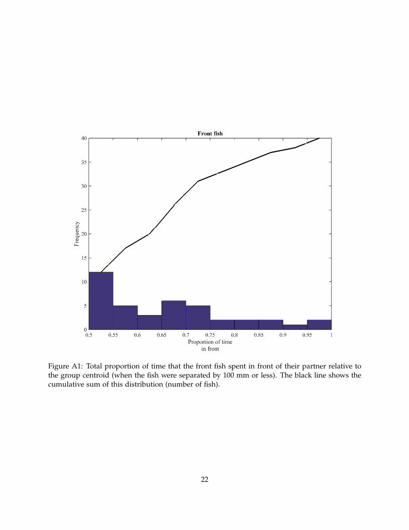
Figure A1: Total proportion of time that the front fish spent in front of their partner relative tothe group centroid (when the fish were separated by 100 mm or less). The black line shows thecumulative sum of this distribution (number of fish).

22

Figure A2: (A) The relative frequency of unbroken durations (segments) spent at the front ofthe pair by either a front fish or back fish. Note there are many instances of individuals onlyoccupying the front position for short periods of time. However, as shown in B, these shortswitches contribute negligible amounts of data to our analysis. (B) shows the contribution thatsegments of different length (x-axis) make towards the data set.

23

Time lag associated with maximum directional correlation

Tables A3 and A4 detail the time lag associated with maximum directional correlation and thecorresponding maximum directional correlation for all 40 groups of fish. Figure A3 contains anexample of directional correlation delay plots for periods spent at the front and rear of a givenpair of fish (group 5).

Table A3: Time lag associated with maximum directional correlation, τ∗ij , and maximum direc-

tional correlation, Cij

(τ∗ij

), for when either fish 1 or fish 2 occupied the front-most position of

the group (groups 1 to 20).

τ∗ij Cij

(τ∗ij

)Group Fish 1 Fish 1 Fish 2 Fish 2 Fish 1 Fish 1

in front behind in front behind in front behind(Fish 2 (Fish 2behind) in front)

1 0.700 -0.550 0.550 -0.700 0.9335 0.91012 0.875 -0.875 0.875 -0.875 0.8828 0.89963 0.750 -0.875 0.875 -0.750 0.9162 0.88944 0.950 -0.650 0.650 -0.950 0.9242 0.89265 0.850 -0.675 0.675 -0.850 0.8588 0.88076 1.475 -1.100 1.100 -1.475 0.9177 0.74037 -3.000 -2.475 2.475 3.000 0.6368 0.98538 0.700 -0.675 0.675 -0.700 0.9009 0.88719 0.825 -0.900 0.900 -0.825 0.8298 0.882710 0.625 -0.875 0.875 -0.625 0.9418 0.822511 1.125 -0.400 0.400 -1.125 0.8804 0.895612 0.575 -0.875 0.875 -0.575 0.8783 0.724613 1.575 -1.575 1.575 -1.575 0.8755 0.797914 -2.400 -1.150 1.150 2.400 0.9734 0.782915 0.675 -0.675 0.675 -0.675 0.9246 0.898316 1.050 -0.675 0.675 -1.050 0.8940 0.830617 0.700 -0.700 0.700 -0.700 0.8587 0.912718 1.200 -1.150 1.150 -1.200 0.7852 0.788019 1.000 -1.050 1.050 -1.000 0.4320 0.749920 0.925 -0.800 0.800 -0.925 0.8497 0.8718

24

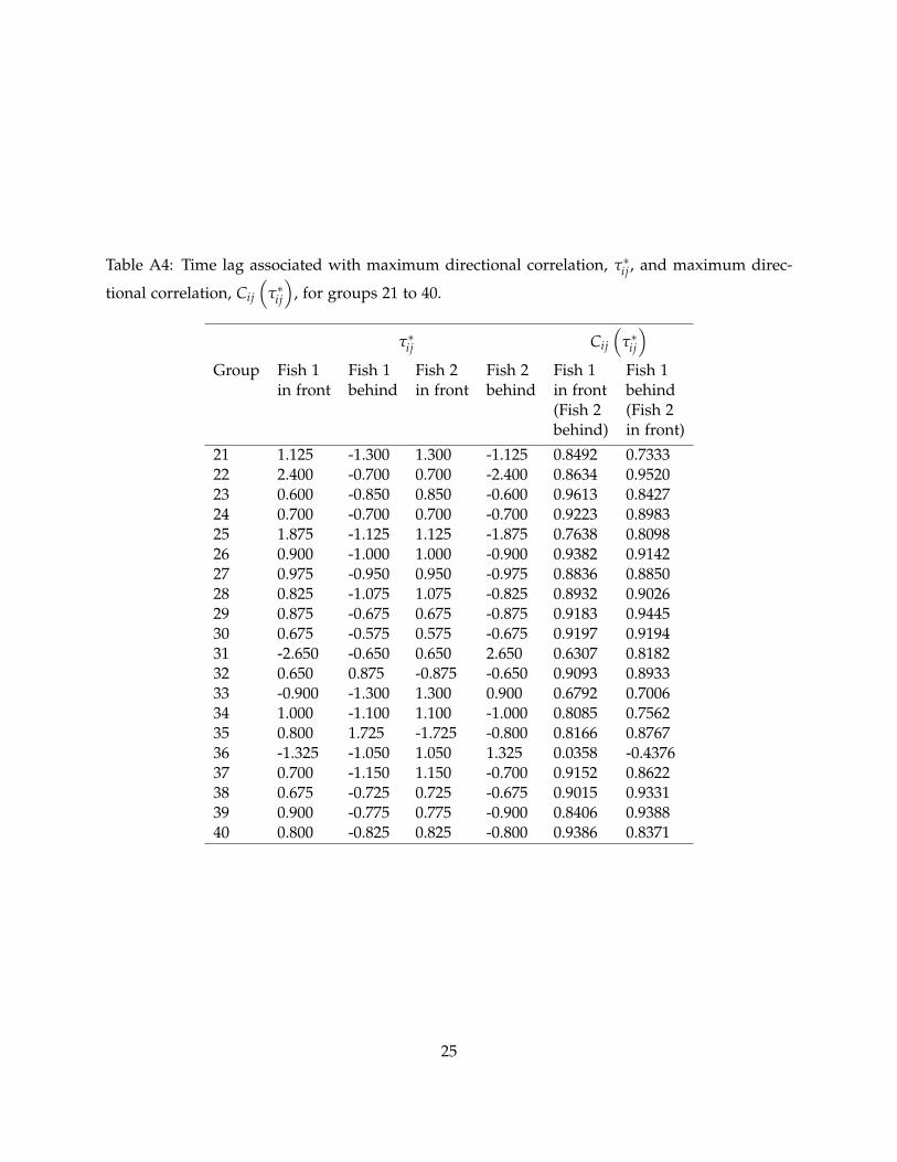
Table A4: Time lag associated with maximum directional correlation, τ∗ij , and maximum direc-

tional correlation, Cij

(τ∗ij

), for groups 21 to 40.

τ∗ij Cij

(τ∗ij

)Group Fish 1 Fish 1 Fish 2 Fish 2 Fish 1 Fish 1

in front behind in front behind in front behind(Fish 2 (Fish 2behind) in front)

21 1.125 -1.300 1.300 -1.125 0.8492 0.733322 2.400 -0.700 0.700 -2.400 0.8634 0.952023 0.600 -0.850 0.850 -0.600 0.9613 0.842724 0.700 -0.700 0.700 -0.700 0.9223 0.898325 1.875 -1.125 1.125 -1.875 0.7638 0.809826 0.900 -1.000 1.000 -0.900 0.9382 0.914227 0.975 -0.950 0.950 -0.975 0.8836 0.885028 0.825 -1.075 1.075 -0.825 0.8932 0.902629 0.875 -0.675 0.675 -0.875 0.9183 0.944530 0.675 -0.575 0.575 -0.675 0.9197 0.919431 -2.650 -0.650 0.650 2.650 0.6307 0.818232 0.650 0.875 -0.875 -0.650 0.9093 0.893333 -0.900 -1.300 1.300 0.900 0.6792 0.700634 1.000 -1.100 1.100 -1.000 0.8085 0.756235 0.800 1.725 -1.725 -0.800 0.8166 0.876736 -1.325 -1.050 1.050 1.325 0.0358 -0.437637 0.700 -1.150 1.150 -0.700 0.9152 0.862238 0.675 -0.725 0.725 -0.675 0.9015 0.933139 0.900 -0.775 0.775 -0.900 0.8406 0.938840 0.800 -0.825 0.825 -0.800 0.9386 0.8371

25

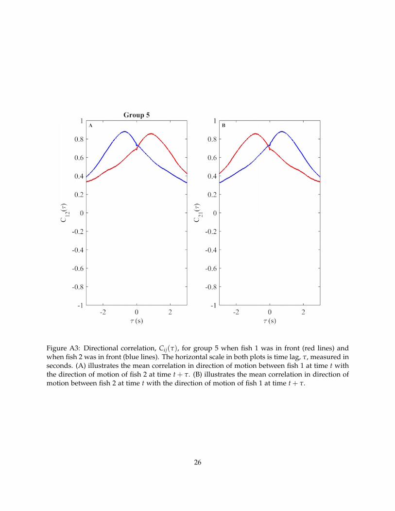
Figure A3: Directional correlation, Cij(τ), for group 5 when fish 1 was in front (red lines) andwhen fish 2 was in front (blue lines). The horizontal scale in both plots is time lag, τ, measured inseconds. (A) illustrates the mean correlation in direction of motion between fish 1 at time t withthe direction of motion of fish 2 at time t + τ. (B) illustrates the mean correlation in direction ofmotion between fish 2 at time t with the direction of motion of fish 1 at time t + τ.

26

Comparison of basic movement statistics

Table A5 summarises the results of statistical tests to determine if there were any differences insummary statistics for properties of movement or body length between individuals that occupiedthe frontmost position of the pair when closely grouped (within 100 mm of each other). Testresults were sorted in ascending order of p-value, and significance levels for each test wereadjusted according to a Holm-Bonferroni correction Holm 1979 (see the fifth column of tableA5). In the absence of a Holm-Bonferroni correction, fish that occupied the frontmost positionfor the greatest duration (compared to their partner) differed from their partner in mean changein speed over time (median difference (front fish minus back fish) in mean change in speedover time = 6.5340 mm/s2), inter-quartile range of speed (mean difference in IQR of speed =5.0105 mm/s), body length (mean difference in body length = 1.0608 mm), median turningspeed (median difference in median turning speed = -6.2436◦/s) and standard deviation in speed(median difference in standard deviation of speed = 1.5169 mm/s). With a Holm-Bonferronicorrection active, only differences in mean change in speed over time remained significant.

Table A5: Results of paired statistical tests applied to summary statistics of locomotive propertiesand body lengths of fish that occupied the front or back of their pair for the greatest proportionof frames when closely grouped (≤ 100 mm from each other). (Locomotive properties exam-ined were speed (si(t)), change in speed over time ( ∆si

∆t ), magnitude of acceleration (ai(t)) andturning speed (αi(t)).) Differences between each summary statistic for each pair of fish werefirst determined. The distribution of these differences were tested for departures from normal-ity using a Shapiro-Wilk test. If the differences were likely to have been drawn from a normaldistribution, then data was further tested using a paired t-test (to determine if the mean of thedifferences differed from zero). If the differences were not normally distributed, then data wasfurther tested according to a Wilcoxon signed rank test as applied by MATLAB’s intrinsic sign-rank function (to determined if the median of the differences departed from zero). Test resultsare sorted in ascending p-value, with appropriate significance levels αsig adjusted according toa Holm-Bonferroni correction listed in the fourth column. All t-tests had 39 degrees of freedom.

Summary Method of Test statistics p αsigstatistic comparison

Mean∆si∆t (t) signed rank test W = 716, z = 4.1130 3.9049× 10−5 0.024

IQR si(t) t-test τ = 3.0744 0.0038 0.0025Body length t-test τ = 2.9633 0.0052 0.0026Median αi(t) signed rank test W = 237, z = −2.3253 0.0201 0.0028Std si(t) signed rank test W = 556, z = 1.9624 0.0497 0.0029Median si(t) signed rank test W = 532, z = 1.6398 0.1010 0.0031Mean si(t) signed rank test W = 518, z = 1.4517 0.1466 0.0033

IQR∆si∆t (t) signed rank test W = 303, z = −1.4382 0.1504 0.0036

Median ai(t) t-test τ = −1.3317 0.1907 0.0038IQR αi(t) signed rank test W = 325, z = −1.1425 0.2532 0.0042

Median∆si∆t (t) signed rank test W = 482, z = 0.9678 0.3332 0.0045

Maximum ai(t) signed rank test W = 469, z = 0.7930 0.4278 0.0050IQR ai(t) signed rank test W = 366, z = −0.5914 0.5542 0.0056Mean ai(t) t-test τ = −0.5151 0.6094 0.0063Mean αi(t) signed rank test W = 382, z = −0.3764 0.7067 0.0071Std αi(t) t-test τ = 0.3718 0.7120 0.0083

Std∆si∆t (t) t-test τ = −0.2848 0.7773 0.0100

Maximum αi(t) signed rank test W = 211, z = −0.1406 0.8882 0.0125Maximum si(t) signed rank test W = 416, z = 0.0806 0.9357 0.0167

Maximum∆si∆t (t) signed rank test W = 405, z = −0.0672 0.9464 0.0250

Std ai(t) signed rank test W = 407, z = −0.0403 0.9678 0.0500

27

Distributions of movement parameters and body lengths

Figure A4: The distribution of observed speeds (in mm/s) for fish that spent the greatest pro-portion of their time at the front (A) or back (B) of each pair when the fish were ≤ 100 mm apart(pooled from all 40 trials).

28

Figure A5: Boxplots of the mean (A), median (B), maximum (C), standard deviation (D) andinter-quartile range (E) of speed (in mm/s) for fish that occupied the front (F) or back (B) of apair for the greatest duration when the fish were ≤ 100 mm apart.

29

Figure A6: The distribution of observed turning speeds (in ◦/s) for fish that spent the greatestproportion of their time at the front (A) or back (B) of each pair when the fish were ≤ 100 mmapart (pooled from all 40 trials).

30

Figure A7: Boxplots of the mean (A), median (B), maximum (C), standard deviation (D) andinter-quartile range (E) of turning speed (in ◦/s) for fish that occupied the front (F) or back (B) ofa pair for the greatest duration when the fish were ≤ 100 mm apart.

31

Figure A8: The distribution of observed magnitudes of acceleration (in mm/s2) for fish that spentthe greatest proportion of their time at the front (A) or back (B) of each pair when the fish were≤ 100 mm apart (pooled from all 40 trials).

32

Figure A9: Boxplots of the mean (A), median (B), maximum (C), standard deviation (D) andinter-quartile range (E) of magnitudes of acceleration (in mm/s2) for fish that occupied the front(F) or back (B) of a pair for the greatest duration when the fish were ≤ 100 mm apart.

33

Figure A10: The distribution of observed changes in speed over time (in mm/s2) for fish thatspent the greatest proportion of their time at the front (A) or back (B) of each pair when the fishwere ≤ 100 mm apart (pooled from all 40 trials).

34

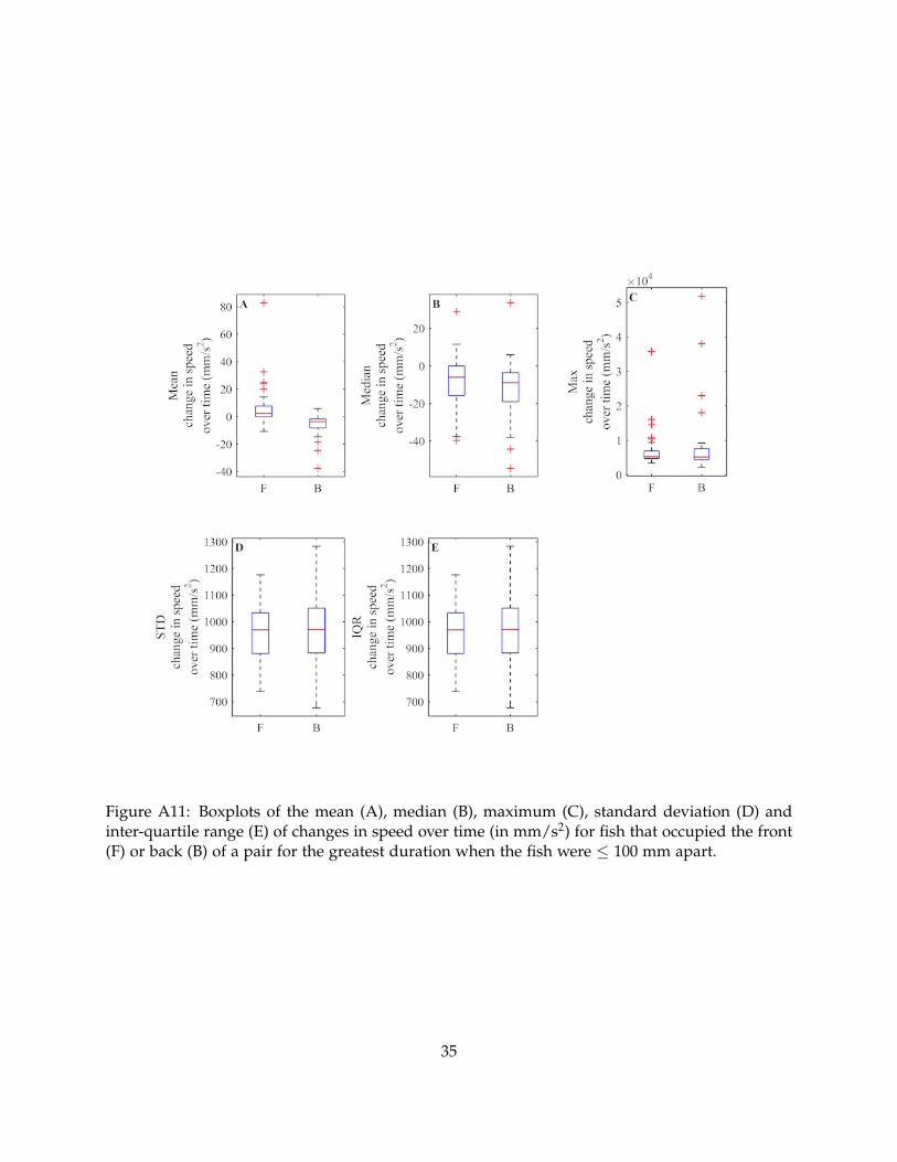
Figure A11: Boxplots of the mean (A), median (B), maximum (C), standard deviation (D) andinter-quartile range (E) of changes in speed over time (in mm/s2) for fish that occupied the front(F) or back (B) of a pair for the greatest duration when the fish were ≤ 100 mm apart.

35

Figure A12: Boxplots of body length (in mm) for fish that occupied the front (F) or back (B) of apair for the greatest duration when the fish were ≤ 100 mm apart.

36

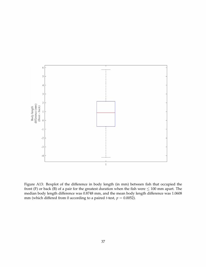
Figure A13: Boxplot of the difference in body length (in mm) between fish that occupied thefront (F) or back (B) of a pair for the greatest duration when the fish were ≤ 100 mm apart. Themedian body length difference was 0.8748 mm, and the mean body length difference was 1.0608mm (which differed from 0 according to a paired t-test, p = 0.0052).

37

Proportion of encounters, speed, relative direction of motion and rules of motion as afunction of relative neighbour location

Figures A14 to A21 illustrate the proportion of encounters, speed, relative direction of motionof partner fish, change in speed over time and change in angle of motion over time for fish thatoccupied the front or back of their pair for the longest duration as a function of relative neighbourlocation. Probabilities determined to examine the likelihood that the sign and magnitude ofobserved differences between front fish and back fish associated quantities might appear throughrandom assignation of front fish and back fish tags were similar irrespective of being derivedfrom either the set of 100 random allocations or the set of 1000 random allocations. Figure A22illustrates the change in speed over time and the change in angle of motion over time of frontand back fish projected onto the y-axis when partner fish are approximately beside a given focalfish (such that −32 < x ≤ 32 (mm), a maximum difference between the approximate centres ofthe fish of approximately one body length).

38

Figure A14: Proportion of total encounters with partner fish projected onto the x-axis (A) and they-axis (B). x or y coordinates on the horizontal axis of the graphs represent the x or y coordinatesof partner fish relative to the location and direction of motion of a given focal fish type. Thecurves show the proportion of encounters where a front fish’s (red curve) or back fish’s (bluecurve) neighbour was observed. The middle panels illustrate the front fish minus the back fishproportion of encounters projected onto the x (C) and y-axes (D). (E) and (F) illustrate the esti-mated probability of a difference at least the same magnitude and sign as that observed occurringif fish were randomly allocated to the set of front fish or back fish. Probabilities estimated froma set of 100 randomisation processes are plotted as dashed lines and probabilities derived from1000 randomisations are plotted as solid lines. Grey regions indicate where estimated probabili-ties derived from 1000 randomisation processes are less than 0.05.

39

Figure A15: (A) and (B) show heat maps of mean speed (mm/s) as a function of the locationof partner fish relative to the direction of motion and position of a focal fish type (front fish orback fish). Focal fish are located at the origin of each plot, moving in the direction of the positivex-axis. (C) contains the difference obtained from the front fish focused map minus the back fishfocused map. Back fish travel slower than front fish when their partner is behind them.

40

Figure A16: Mean speed of focal fish as a function of their partner’s x- (A) or y-coordinate (B).Curves representing the mean speed of front fish are plotted in red; curves representing the meanspeed of back fish are plotted in blue. Dashed lines are plotted one standard error above andbelow mean speed curves. (C) and (D) illustrate the difference in front fish and back fish curves,and (E) and (F) illustrate the estimated probability of a difference at least the same magnitudeand sign as that observed occurring. Probabilities estimated from a set of 100 randomisationprocesses are plotted as dashed lines and probabilities derived from 1000 randomisations areplotted as solid lines. Grey regions indicate where estimated probabilities derived from 1000randomisation processes are less than 0.05. Back fish are slower than front fish when theirpartner is behind them.

41

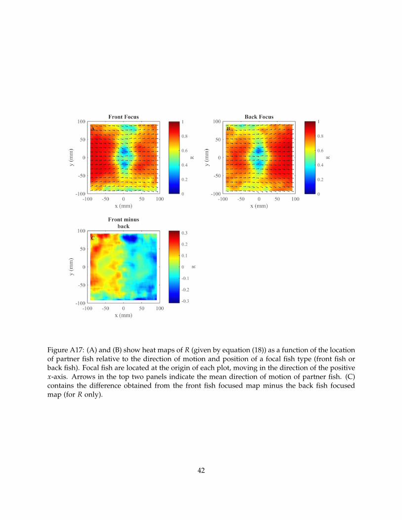
Figure A17: (A) and (B) show heat maps of R (given by equation (18)) as a function of the locationof partner fish relative to the direction of motion and position of a focal fish type (front fish orback fish). Focal fish are located at the origin of each plot, moving in the direction of the positivex-axis. Arrows in the top two panels indicate the mean direction of motion of partner fish. (C)contains the difference obtained from the front fish focused map minus the back fish focusedmap (for R only).

42

Figure A18: (A) and (B) show heat maps of mean change in speed (mm/s2) (the instantaneouschange in magnitude of a fish’s velocity vector) as a function of the location of their neighbourrelative to the direction of motion and position of a focal fish type (front fish or back fish). Focalfish are located at the origin of each plot, moving in the direction of the positive x-axis. Extremevalues for the mean change in speed have been truncated at ±120mm/s2 in the top two panelsto allow for better visualisation of the details of lower magnitude changes in speed. (C) containsthe difference obtained from the front fish focused map minus the back fish focused map.

43

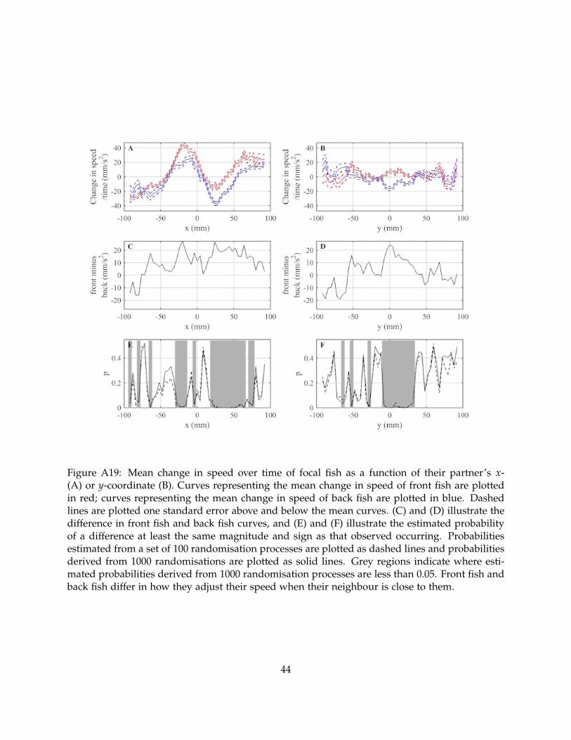
Figure A19: Mean change in speed over time of focal fish as a function of their partner’s x-(A) or y-coordinate (B). Curves representing the mean change in speed of front fish are plottedin red; curves representing the mean change in speed of back fish are plotted in blue. Dashedlines are plotted one standard error above and below the mean curves. (C) and (D) illustrate thedifference in front fish and back fish curves, and (E) and (F) illustrate the estimated probabilityof a difference at least the same magnitude and sign as that observed occurring. Probabilitiesestimated from a set of 100 randomisation processes are plotted as dashed lines and probabilitiesderived from 1000 randomisations are plotted as solid lines. Grey regions indicate where esti-mated probabilities derived from 1000 randomisation processes are less than 0.05. Front fish andback fish differ in how they adjust their speed when their neighbour is close to them.

44

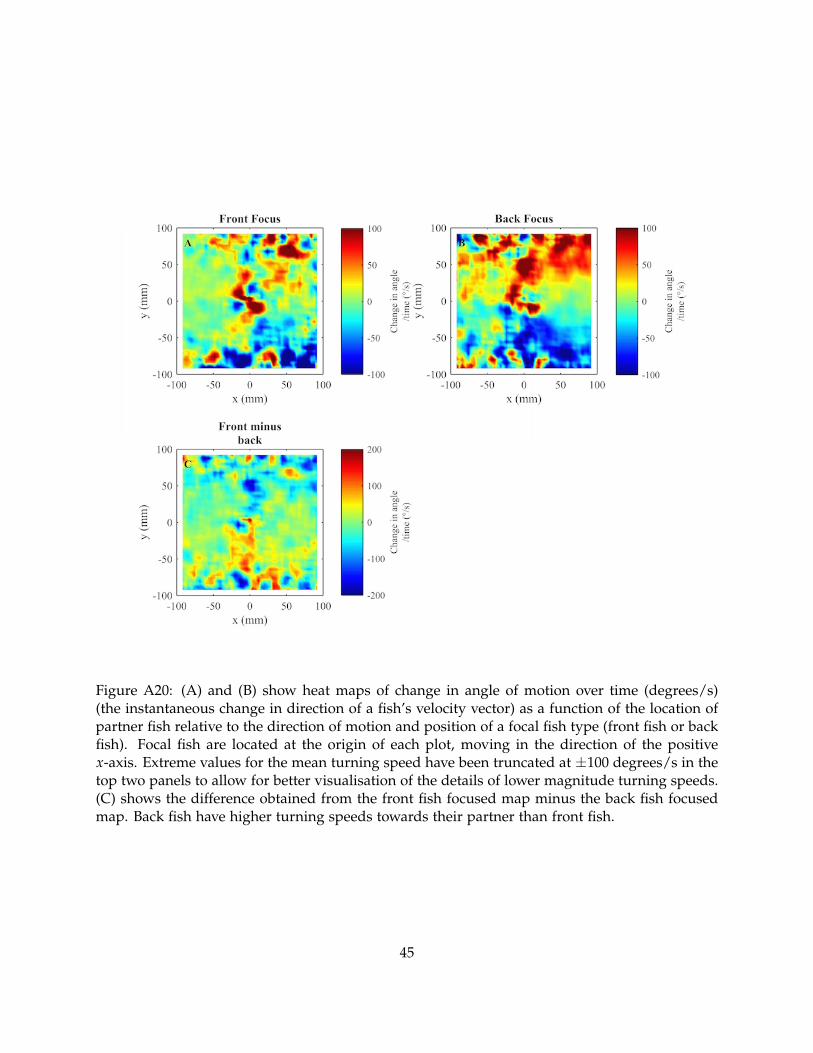
Figure A20: (A) and (B) show heat maps of change in angle of motion over time (degrees/s)(the instantaneous change in direction of a fish’s velocity vector) as a function of the location ofpartner fish relative to the direction of motion and position of a focal fish type (front fish or backfish). Focal fish are located at the origin of each plot, moving in the direction of the positivex-axis. Extreme values for the mean turning speed have been truncated at ±100 degrees/s in thetop two panels to allow for better visualisation of the details of lower magnitude turning speeds.(C) shows the difference obtained from the front fish focused map minus the back fish focusedmap. Back fish have higher turning speeds towards their partner than front fish.

45

Figure A21: Mean change in angle of motion over time of focal fish as a function of their partner’sx- (A) or y-coordinate (B). Curves representing the mean turning speed of front fish are plotted inred; curves representing the mean turning speed of back fish are plotted in blue. Dashed lines areplotted one standard error above and below the mean curves. Positive values of turning speedindicate are associated with anti-clockwise turns; negative values are associated with clockwiseturns. (C) and (D) illustrate the difference in front fish and back fish curves, and (E) and (F)illustrate the estimated probability of a difference at least the same magnitude and sign as thatobserved occurring. Probabilities estimated from a set of 100 randomisation processes are plottedas dashed lines and probabilities derived from 1000 randomisations are plotted as solid lines.Grey regions indicate where estimated probabilities derived from 1000 randomisation processesare less than 0.05.

46

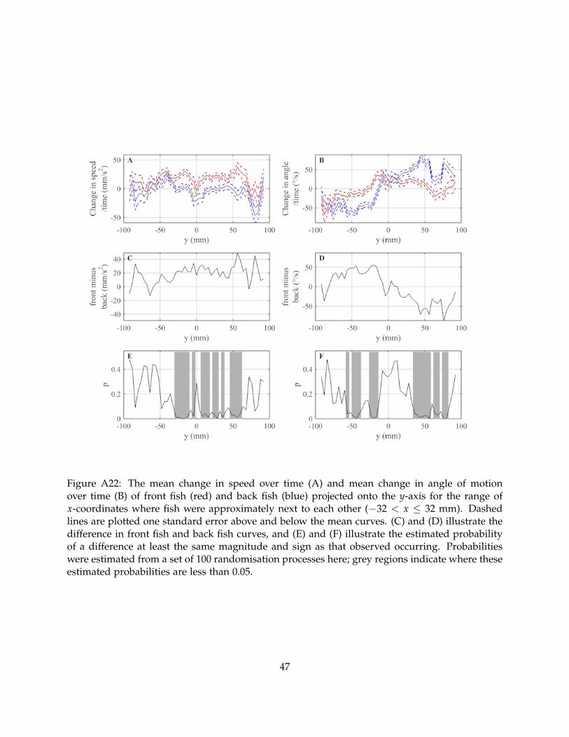
Figure A22: The mean change in speed over time (A) and mean change in angle of motionover time (B) of front fish (red) and back fish (blue) projected onto the y-axis for the range ofx-coordinates where fish were approximately next to each other (−32 < x ≤ 32 mm). Dashedlines are plotted one standard error above and below the mean curves. (C) and (D) illustrate thedifference in front fish and back fish curves, and (E) and (F) illustrate the estimated probabilityof a difference at least the same magnitude and sign as that observed occurring. Probabilitieswere estimated from a set of 100 randomisation processes here; grey regions indicate where theseestimated probabilities are less than 0.05.

47