identifying runoff routing parameters for operational ... · identifying runoff routing parameters...

Hydrological Sciences–Journal–des Sciences Hydrologiques, 53(1) February 2008

Open for discussion until 1 August 2008 Copyright © 2008 IAHS Press

112

Identifying runoff routing parameters for operational flood forecasting in small to medium sized catchments CHRISTIAN RESZLER, GÜNTER BLÖSCHL & JÜRGEN KOMMA Institute for Hydraulic and Water Resources Engineering, University of Technology Vienna, Karlsplatz 13/222, A-1040 Wien, Austria Abstract This paper proposes a framework for identifying the parameters of a lumped routing model in small to medium sized catchments where lateral inflows can be large but poorly defined. In a first step, a priori estimates of the parameters are made based on topography, aerial photographs, flood marks and field surveys. In a second step, runoff data are analysed of reservoir release events and convective events where no rainfall in the direct catchments occurred. In a third step the routing model is calibrated to the results of hydrodynamic models for scenarios of different magnitudes. In a fourth step, these pieces of information are combined, allowing for soft expert judgement to be incorporated. In a fifth step, the routing parameters are fine tuned to observed flood events where lateral inflows are estimated by a rainfall–runoff model. The framework is illustrated by the Kamp flood forecasting system in Austria that has been in operational use since 2006. Key words flow routing; parameter identification; hydrological model; operational flood forecasting

Identification de paramètres de propagation d’écoulement pour la prévision opérationnelle de crue au sein de bassins versants de petite à moyenne taille Résumé Cet article propose une démarche pour identifier les paramètres d’un modèle global de propagation dans des bassins versants de petite à moyenne taille, où les afflux latéraux peuvent être importants mais mal définis. En première étape, des estimations a priori des paramètres sont faites à partir de la topographie, de photographies aériennes, de laisses de crues et d’enquêtes de terrain. Dans une deuxième étape, les données de débit sont analysées pour des événements de lâchure de barrage et des événements convectifs lors desquels aucune pluie n’est tombée sur les bassins directs. Dans une troisième étape, le modèle de propagation est calé à l’aide des résultats de modèles hydrodynamiques pour des scénarios d’amplitudes variables. Dans une quatrième étape, ces éléments d’information sont combinés, permettant d’incorporer des avis d’expert nuancés. Dans une cinquième étape, les paramètres de propagation sont affinés par rapport à des événements de crue observés pour lesquels les afflux latéraux sont estimés par un modèle pluie–débit. La démarche est illustrée avec le système de prévision de crue autrichien de Kamp qui est opérationnel depuis 2006. Mots clefs propagation de crue; identification de paramètre; modèle hydrologique; prévision opérationnelle de crue INTRODUCTION

Numerous methods exist for flood routing in natural river reaches. The choice of method depends on data availability and on the type of application. Hydrodynamic models based on the de St Venant equations are typically used for analysing flood events in applications such as estimating design floods, evaluating the effects of flood retention measures and for estimating flood risk zones in a land-use planning context. The advantage of hydrodynamic models is that changes in the geometry can be explicitly incorporated, extrapolation to very large floods is possible, and inundation patterns and flow velocities can be estimated. However, they need detailed input data of the channel geometry, roughness and lateral inputs. Also, they are typically computationally demanding and numerical stability may be an issue, particularly if flood flow in the flood plains is simulated. For operational flood forecasting, the requirements are different from the analysis case. Numerical stability is of utmost importance and, for many applications, computation times need to be short. The latter is of particular importance if ensemble forecasts are made that simulate a large number of future flood flows to evaluate the uncertainty of the forecasts (Komma et al., 2007). Even though the computational power of computers is increasing steadily there are definite merits of using routing models that are simpler than full hydrodynamic models. This is particularly so for small to medium sized catchments where the flood routing is not necessarily the main part of the forecast system and the representation of runoff generation, based on rainfall–runoff models, is the

Identifying runoff routing parameters for operational flood forecasting

Copyright © 2008 IAHS Press

113

more challenging part. Lumped routing models have hence been widely used in operational flood forecasting systems (e.g. Gutknecht et al., 1997). Lumped routing models were initially developed as linear models and later extended to allow for nonlinear characteristics, mainly to represent flood-plain effects on the hydrograph. Nonlinear models include nonlinear storage–flow relationships (e.g. Laurenson, 1964; Ponce & Yevjevich, 1978; Koussis & Osborne, 1986; Malone & Cordery, 1989) and multi-linear models that represent the routing process as a sequence of linear processes with parameters changing as a function of flood flow. Variants of the latter are the multiple linearisation flow routing model of Keefer & McQuivey (1974), the threshold model (Becker, 1976; Becker & Kundzewicz, 1987) and the multi-linear model of O’Connor (1976) based on a discrete version of a storage cascade. The main advantage of lumped routing models in a flood forecasting context is numerical stability and computational efficiency. Also, as there are usually only a small number of model parameters involved, these can be tested for plausibility to maximise the reliability and credibility of the forecasting procedure. However, these advantages come at the expense that calibration of the model parameters is more important, particularly if the interest resides in forecasting extreme floods where the routing characteristics of the flood plain play an important role. Calibration of the model parameters of lumped flood routing models is usually based on comparing flood runoff data at a streamgauge with those at an upstream gauge (e.g. Wong & Laurenson, 1984; Szolgay, 2004; Mitkova et al., 2005). This works well: – for large rivers where the lateral inflows are small relative to the flow of the main channel, – if flood data are available for the river reaches of interest, and – if those flood data cover the range of flows for which the forecasting system is designed. This is not always the case, in particular when one is interested in flood forecasting in small to medium sized catchments. A number of authors have therefore developed methods for inferring the routing model parameters from the linearised de St Venant model based on simplified channel geometries (Dooge, 1973; Koussis, 1978; Dooge et al., 1982). Alternatively, a hybrid approach has been suggested (e.g. Perumal, 1994) where the lumped routing model is calibrated to the results of a hydrodynamic model. In the context of developing an operational flood forecasting system, other data sources may exist that are relevant for flood routing, including flood marks and aerial photographs, in addition to runoff data and any existing results of hydrodynamic models. It is clear that combining these disparate types of information should help us obtain reliable model parameters but, to the best of our knowledge, no framework exists for doing this. The aim of this paper is to propose a framework for combining disparate sources of information in a structured way to estimate the parameters of a lumped routing model. The idea is to combine the advantages of the lumped routing approach with those of the hydrodynamic approach, i.e. robustness, numerical efficiency and a small number of plausible model parameters on the one hand, and reliable extrapolation to large events, estimation for ungauged river reaches and treatment of lateral inflows, on the other hand. We illustrate the framework by a case study in the Kamp catchment in Austria that uses a nonlinear storage cascade as the lumped routing model. ROUTING MODEL

The response of a linear storage cascade (Nash, 1957) to an instantaneous input U1 of unit volume is:

kt

nnnn t

nkS

kQ

−− ⋅⋅−⋅

=⋅= e)!1(

11 1 (1)

where Qn is the outflow of the cascade, Sn is the storage of the last reservoir, t is the time, n is the number of reservoirs, k the time parameter of each reservoir and n·k is the total travel time.

Christian Reszler et al.


114

The state space notation of Szöllösi-Nagy (1982), Szilagyi (2003) and Szolgay (2004) is used here. The state space notation implies that the entire memory of the model is embodied in the state variable at a single point in time. Future runoff only depends on this state variable. If one assumes that the input vector U to each reservoir is constant within a time interval (i,i – 1) of duration Δt, the reservoir storage and outflow are:

1,1,11, −−−− ⋅+⋅= iiiiiiii UGSFS (2) iii SHQ ⋅= (3)

where S und Q are the (n·1) state vectors of reservoir storages and outflow. H is an (n·n)-matrix that contains the inverse of the time parameter k in the diagonal:

IH ⋅= )/1,...,/1,/1( kkk (4)

where I is the identity matrix. The transition matrices F (state) and G (input) with dimension (n·n) and (n·1), respectively, are defined as:

⎥⎥⎥⎥⎥⎥⎥⎥⎥⎥

⎦

⎤

⎢⎢⎢⎢⎢⎢⎢⎢⎢⎢

⎣

⎡

−−

=

−−−−−

−−

−−

−

−

kt

ktn

ktn

kt

kt

kt

kt

kt

ii

een

tken

tk

teketk

etek

e

ΔΔΔ

ΔΔ

ΔΔ

Δ

ΔΔ

ΔΔ

Δ

L

MOM

L

)!2()(

)!1()(

0!2)(

0

00

21

21,F (5)

⎥⎥⎥⎥⎥⎥⎥⎥⎥

⎦

⎤

⎢⎢⎢⎢⎢⎢⎢⎢⎢

⎣

⎡

⎟⎟

⎠

⎞

⎜⎜

⎝

⎛⎟⎠⎞

⎜⎝⎛−

⎟⎟

⎠

⎞

⎜⎜

⎝

⎛+−

−

=

∑−

=

−

−

−

−

1

0

1,

!11

)1(1

)1(

n

j

jkt

kt

kt

ii

kt

jek

ktek

ek

Δ

Δ

Δ

Δ

Δ

MG (6)

To allow for nonlinear routing, k is allowed to vary as a function of the inflow U1 to the river reach based on the time distribution scheme of Becker & Kundzewicz (1987). Varying k is straightforward in the state space notation as equations (2)–(6) are evaluated for each time step as a function of the states S and Q of the previous time step and the value of k that is consistent with the inflow between the previous time step and the current time step. It is assumed that k is a piecewise linear function of the inflow to the reach, U1. For simplicity, the number of reservoirs n is not allowed to vary with the inflow but does vary between the river reaches. STUDY AREA AND MODEL TOPOLOGY

The Kamp originates in Lower Austria, close to the Czech border, joins the Zwettl stream and the Purzelkamp (Fig. 1) and drains into the Kamp hydropower scheme which consists of the Ottenstein, Dobra and Thurnberg reservoirs. These reservoirs modify the flood regime of the Upper Kamp. Downstream of the hydropower scheme, the Taffa, a northern tributary, joins the Kamp, which then flows from north to south. This reach is termed the Lower Kamp. The total catchment area of the Kamp at Zöbing is 1550 km2. In this study, runoff data of the following streamgauges are used: Kamp at Neustift (77 km2 catchment area), Zwettl (622 km2),



115

Thurn-berg

Rasten-berg

Dobra

Ottenstein

Purzelkamp

Kam

p

Zwettl

Kamp

Kamp

Taffa

Neustift

Rauschermühle

Frauenhofen

Stiefern

Zöbing (outlet)

Rosenburg

1

2 4

10 km

14.9°E

48.7°N

Stream gaugesReservoirs

Sub catchments

Runoff routing reaches(no. 1 - 8)

Zwettl/Kamp5

7

6

8

3

Zwettl/Zwettl

Fig. 1 Kamp catchment with routing reaches and direct catchments indicated.

Rauschermühle (1150 km2) and Stiefern (1493 km2); Zwettl at Zwettl (274 km2); Purzelkamp at Rastenberg (95 km2); Taffa at Frauenhofen (140 km2) and Rosenburg (250 km2). Runoff data at 15-min time steps are available at these gauges from 1977 to 2006, with the exception of Rosenburg where data are available for 2005–2006. Additionally, outflow from the three reservoirs are used, and inflow to the reservoirs has been back-calculated from reservoir level changes. The routing model examined in this paper is part of the KAMPUS flood forecasting model which consists of a rainfall–runoff model and the routing component. The rainfall–runoff model is organised as a grid model with 1 km2 grid resolution and is based on a soil moisture accounting scheme (Reszler et al., 2006; Blöschl et al., 2008). The soil moisture scheme accounts for runoff generation and changes in the soil moisture state of the catchment, and involves three parameters: the maximum soil moisture storage, a parameter representing the soil moisture state above which evaporation is at its potential rate and a parameter in the nonlinear function relating runoff generation to the soil moisture state. Runoff routing on the hillslopes is represented by an upper and two lower soil reservoirs. Excess rainfall enters the upper zone reservoir and leaves this reservoir through three paths: outflow from the reservoir based on a fast storage coefficient; percolation to the lower zone with a constant percolation rate; and, if a threshold of the storage state is exceeded, through an additional outlet based on a very fast storage coefficient. Water leaves the lower zones based on two slow storage coefficients. Fast bypass flow in the soil is accounted for by recharging the lower zone reservoir directly by a fraction of the excess rainfall. The outflow from the reservoirs represents the total runoff on the hillslope scale. Reszler et al. (2006) and Parajka et al. (2005) give more details on the model. Sub-catchment runoff simulated by the rainfall–runoff model is added to each downstream node of the routing model as lateral inflow. The time step of the model, including the routing component is Δt = 15 min. The nodes of the forecasting model have been chosen at the streamgauge locations, important confluences and forecast points. A total of eight routing reaches were selected (Table 1). Reaches 1, 2, 3 and 4 of the Upper Kamp are upstream of the hydropower scheme. The contribution of the direct catchments (lateral inflow) is significant, so for many flood events, the shape of the



116

Table 1 Routing reaches at the Kamp catchment (see Fig. 1). Reach no. Stream Reach Length

(km) Upstream catchment area (km²)

Direct catchment area (km2)

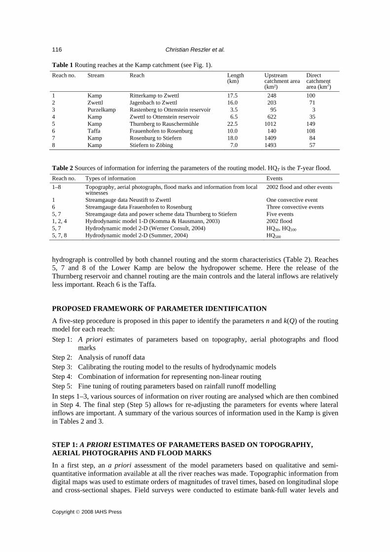
1 Kamp Ritterkamp to Zwettl 17.5 248 100 2 Zwettl Jagenbach to Zwettl 16.0 203 71 3 Purzelkamp Rastenberg to Ottenstein reservoir 3.5 95 3 4 Kamp Zwettl to Ottenstein reservoir 6.5 622 35 5 Kamp Thurnberg to Rauschermühle 22.5 1012 149 6 Taffa Frauenhofen to Rosenburg 10.0 140 108 7 Kamp Rosenburg to Stiefern 18.0 1409 84 8 Kamp Stiefern to Zöbing 7.0 1493 57 Table 2 Sources of information for inferring the parameters of the routing model. HQT is the T-year flood. Reach no. Types of information Events 1–8 Topography, aerial photographs, flood marks and information from local

witnesses 2002 flood and other events

1 Streamgauge data Neustift to Zwettl One convective event 6 Streamgauge data Frauenhofen to Rosenburg Three convective events 5, 7 Streamgauge data and power scheme data Thurnberg to Stiefern Five events 1, 2, 4 Hydrodynamic model 1-D (Komma & Hausmann, 2003) 2002 flood 5, 7 Hydrodynamic model 2-D (Werner Consult, 2004) HQ30, HQ100 5, 7, 8 Hydrodynamic model 2-D (Summer, 2004) HQ500 hydrograph is controlled by both channel routing and the storm characteristics (Table 2). Reaches 5, 7 and 8 of the Lower Kamp are below the hydropower scheme. Here the release of the Thurnberg reservoir and channel routing are the main controls and the lateral inflows are relatively less important. Reach 6 is the Taffa. PROPOSED FRAMEWORK OF PARAMETER IDENTIFICATION

A five-step procedure is proposed in this paper to identify the parameters n and k(Q) of the routing model for each reach: Step 1: A priori estimates of parameters based on topography, aerial photographs and flood

marks Step 2: Analysis of runoff data Step 3: Calibrating the routing model to the results of hydrodynamic models Step 4: Combination of information for representing non-linear routing Step 5: Fine tuning of routing parameters based on rainfall runoff modelling In steps 1–3, various sources of information on river routing are analysed which are then combined in Step 4. The final step (Step 5) allows for re-adjusting the parameters for events where lateral inflows are important. A summary of the various sources of information used in the Kamp is given in Tables 2 and 3. STEP 1: A PRIORI ESTIMATES OF PARAMETERS BASED ON TOPOGRAPHY, AERIAL PHOTOGRAPHS AND FLOOD MARKS

In a first step, an a priori assessment of the model parameters based on qualitative and semi-quantitative information available at all the river reaches was made. Topographic information from digital maps was used to estimate orders of magnitudes of travel times, based on longitudinal slope and cross-sectional shapes. Field surveys were conducted to estimate bank-full water levels and



117

Table 3 Availability of information for inferring the parameters of the routing model for each of the river reaches. Reach no. Step 1:

A priori information

Step 2: Runoff data

Step 3: Hydrodynamic model

Step 5: Fine tuning by rainfall–runoff model

1 x x x x 2 x x x 3 x x 4 x x x 5 x x x x 6 x x x 7 x x x x 8 x x x bank-full discharges. This is important, as the change in the time parameter k once the flood plain starts to flood is important in representing flood routing. Also, topographic information both from the maps and the field surveys was used to assess retention areas. As actual inundation areas are more accurate than a terrain analysis, several pieces of information from past large floods were analysed, in particular flood marks and aerial photographs, to assist in the assessment of inundation areas. Discussions and short interviews with local witnesses of past floods were also conducted. Below, examples of the procedure are given for two reaches of the Upper Kamp (reaches 1 and 2) and two reaches of the Lower Kamp (reaches 5 and 7). Information from the August 2002 flood in the Kamp area, estimated to be a 500-year flood, was used. Reach 1 of the Upper Kamp is relatively steep; Reach 2 is wider and flatter. Also, the inundation areas of Reach 2 are much larger as indicated by the topographic assessment from both maps and field surveys. The lengths of the two reaches are similar (Table 1) so significantly larger travel times would be expected for Reach 2. A rough estimate of typical celerity at Reach 1 of about 1–2 m/s for low flow gives travel times of 2.5–5 h. For high in-channel flow, the celerity is likely to be larger (1.5–3 m/s), which translates into travel times of about 1.5–3 h. In Reach 1, inundation effects on the travel time are likely to exist, suggesting that the travel time increase once bank-full discharge is exceeded. However, the effects are probably not very large as the valley is rather narrow. Travel times of Reach 2 are about 1.5 times those of Reach 1 and the inundation effects are probably more pronounced. Analyses of aerial photographs of the 2002

Fig. 2 Flood marks of the August 2002 flood at the bank of the Kamp near Rosenburg (Reach 5). The peak flow was about 570 m³/s. Photo courtesy of Pfarre Horn.



118

flood around the town of Zwettl confirmed the large inundation areas in Reach 2. Analyses of the August 2002 flood data of the Zwettl streamgauge (Reach 2) indicate that, at flows exceeding about 100 m3/s, the hydrograph remained constant over some time. This, along with the aerial photographs, suggests that this is the discharge where substantial inundation starts in this part of the reach. The valley of Reach 5 of the Lower Kamp downstream of the hydropower scheme is narrow and the side slopes are forested. Figure 2 shows traces of the August 2002 flood in the vicinity of the town of Rosenburg, near the downstream node of Reach 5. The building had been inundated up to the middle of the windows suggesting that the water level of the flood was about 4 m above normal. However, the valley is relatively narrow in this reach, so the inundation areas are rather small. The photo shows the side slope of the valley that is close to the building. For this type of profile, one would expect that the flow celerity increases with discharge but, as no inundation into a flood plain occurs, the celerities will likely not decrease above a critical threshold. Along reaches 7 and 8 downstream of Rosenburg, much of the channel is regulated and the valley is relatively narrow. The valley is more densely populated than the upper reaches of the Kamp, so much of the area close to the river is built up. Figure 3 gives an example of the stream near the upstream node of Reach 7 at Gars during a small flood in July 2005. The discharge was 75 m3/s which corresponds to bank-full discharge. The flood plains are flooded slightly above this discharge (at about 80 m3/s). However, the total area of the flood plains is relatively small, so one would not expect a drastic change in the routing characteristics as the flow exceeds bank-full discharge.

Fig. 3 Kamp between Rosenburg and Stiefern during the event in July 2005 (Reach 7). The discharge was about 75 m3/s which is almost bank full discharge.

A priori estimates of the parameters for the remaining river reaches have been obtained in a similar fashion. These estimates were used both as a starting point for the calibration in the following steps and as a plausibility check, in particular when extrapolating the parameters to large flood discharges. STEP 2: ANALYSIS OF RUNOFF DATA

For large rivers where the lateral inflows are small relative to the flow of the main channel, estimating the parameters of routing models is relatively straightforward. However, for small to



119

medium sized catchments, lateral inflows can be relatively much larger, so changes in the shape of the hydrograph cannot be traced back uniquely to channel routing. The idea of the proposed framework is to select those observed events for parameter estimation where lateral inflows were indeed small. There are, typically, two types of events that can be used for this purpose. The first are convective events where the rain storm is limited to a relatively small area upstream of the reach to be analysed, with very little or no rainfall in the direct catchment of the reach. The second type are events where changes in the streamflow are of anthropogenic origin, e.g. due to reservoir releases. Release operation of hydro-electric power schemes during non-flood situations is usually controlled by the electricity market rather than by hydrological constraints, so there are many cases where discharge fluctuations occur without any rainfall in the direct catchment of the reach. Events of different magnitudes need to be analysed to identify the nonlinearity of the routing process. In catchments such as the Kamp, however, both convective events and reservoir release events are small while the large events are produced by abundant rainfall over a larger area. This means that analyses of the runoff data can be used to estimate the parameters of the routing model at the lower end of the discharge range. Parameters for large discharges need to be obtained from alternative sources. As most events in the Kamp are associated with rainfall over a large region, only a small number of events was available for analysis. At the Upper Kamp, only a single event in each of reaches 1 and 2 could be used. At the Lower Kamp, a total of five events could be used. These include larger events where the lateral inflow was relatively small as well as reservoir release events. Figure 4 provides an example of the calibration of the routing model to a small convective event at the Taffa (Reach 6) on 12 September 2005. This event is very well suited to calibrating the parameters of the model as all of the rain fell upstream of the Frauenhofen gauge and there was no rainfall in the direct catchment. Fitting the model to the hydrograph gave n = 15 and n·k = 1.3 h assuming, for robustness of parameter estimation, that the parameters are constant during the event. Figure 5 shows an example of a reservoir release event, observed at the Lower Kamp between Rauschermühle and Stiefern. The Rauschermühle gauge is 2 km upstream of the upstream node of

Rosenburg calibrated

Rosenburg observed

Frauenhofen(Input)

Time (hours)

Q (m

³/s)

Fig. 4 Calibrating the routing model to a convective event on 12 September 2005 at Reach 6 (Taffa). Parameters found are n = 15 and n⋅k = 1.3 h.



120

Stiefern

4-5 h

4-5 h

Time (hours)

Q (m

³/s) Rauschermühle

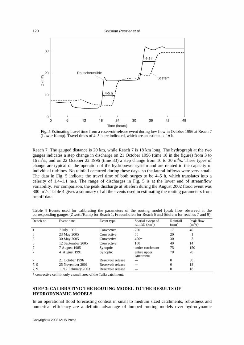
Fig. 5 Estimating travel time from a reservoir release event during low flow in October 1996 at Reach 7 (Lower Kamp). Travel times of 4–5 h are indicated, which are an estimate of n⋅k.

Reach 7. The gauged distance is 20 km, while Reach 7 is 18 km long. The hydrograph at the two gauges indicates a step change in discharge on 21 October 1996 (time 18 in the figure) from 3 to 16 m3/s, and on 22 October 22 1996 (time 33) a step change from 16 to 30 m3/s. These types of change are typical of the operation of the hydropower system and are related to the capacity of individual turbines. No rainfall occurred during these days, so the lateral inflows were very small. The data in Fig. 5 indicate the travel time of both surges to be 4–5 h, which translates into a celerity of 1.4–1.1 m/s. The range of discharges in Fig. 5 is at the lower end of streamflow variability. For comparison, the peak discharge at Stiefern during the August 2002 flood event was 800 m3/s. Table 4 gives a summary of all the events used in estimating the routing parameters from runoff data. Table 4 Events used for calibrating the parameters of the routing model (peak flow observed at the corresponding gauges (Zwettl/Kamp for Reach 1, Frauenhofen for Reach 6 and Stiefern for reaches 7 and 9). Reach no. Event date Event type Spatial extent of

rainfall (km2) Rainfall (mm)

Peak flow (m3/s)

1 7 July 1999 Convective 200 17 40 6 23 May 2005 Convective 50 20 1 6 30 May 2005 Convective 400* 30 3 6 12 September 2005 Convective 100 40 14 7 7 August 1985 Synoptic entire catchment 75 150 7 4 August 1991 Synoptic entire upper

catchment 70 70

7 21 October 1996 Reservoir release --- 0 30 7, 9 25 November 2001 Reservoir release --- 0 18 7, 9 11/12 February 2003 Reservoir release --- 0 18 * convective cell hit only a small area of the Taffa catchment. STEP 3: CALIBRATING THE ROUTING MODEL TO THE RESULTS OF HYDRODYNAMIC MODELS

In an operational flood forecasting context in small to medium sized catchments, robustness and numerical efficiency are a definite advantage of lumped routing models over hydrodynamic



121

models. However, in terms of extrapolation to large events and estimation for ungauged river reaches, hydrodynamic models have clear advantages. The idea of this step of the proposed framework is to combine the merits of the two approaches by calibrating the lumped routing model to the results of hydrodynamic models. As hydrodynamic models are based on the de St Venant equations and detailed terrain data, the extrapolation to ungauged cross-sections and to discharges larger than those observed is likely to be more reliable than direct extrapolation of the lumped routing model. The scenario runs can be varied over a range of event magnitudes, so the change in the model parameters with discharge can be fully incorporated into the calibration procedure. Also, scenarios can be run without any rainfall, so the lateral inflow will be either zero or very small. The limitation is, of course, that the accuracy of the parameters so obtained hinges on the accuracy of the hydrodynamic model that, similarly, needs some calibration to streamflow data. In many river reaches around the world, calibrated hydrodynamic models have been set up in a flood design or flood risk context and it is more economic to use the results of available models than to calibrate dedicated models in the context of developing a flood forecasting system. This is the case for the Kamp where, in recent years, a number of design studies (Werner Consult, 2004; Summer, 2004) and flood risk analyses (Komma & Hausmann, 2003) have been performed. In each of these studies, a hydrodynamic model has been calibrated to various reaches of the Kamp. For the Upper Kamp, the results of the study of Komma & Hausmann (2003) were used here. They set up the one-dimensional (1-D) HEC RAS model for two reaches (Reach 2, and reaches 1 and 4 combined). The model solves the full de St Venant equations by an implicit finite difference method in unsteady state (USACE, 2002). Terrain profiles spaced at about 600 m were acquired during field surveys and combined with a 10 m terrain model. Komma & Hausmann (2003) made assumptions about lateral inflows and calibrated the HEC RAS model to hydrographs (discharges and water levels) of the two flood events in August 2002 of the Kamp at Zwettl and the Zwettl at Zwettl. The latter gauge is located at Reach 2, 1 km upstream of the confluence of reaches 2 and 1. Additionally, Komma & Hausmann (2003) tested the model with inundation maps obtained from aerial photographs. They then performed a number of scenario runs with the hydrodynamic model. The lumped routing model in this paper was calibrated to these scenarios. Figure 6 shows an example for reaches 1 and 4 combined (24 km). For robustness, again, the parameters of the lumped routing model were assumed constant during an event. The figure indicates that the travel times simulated by the hydrodynamic model indeed decrease with the magnitude of the flow. For the largest scenario a peak discharge of 170 m3/s was simulated by the hydrodynamic model at time 07:00 h, while for the smallest scenario a peak discharge of 20 m3/s was simulated at time 08:00 h. The calibration parameters found from the calibration for the combined reaches 1 and 4 are n = 5 and kn ⋅ = 2 h for the largest scenario and n = 7 and kn ⋅ = 3 h for the smallest scenario. In terms of celerity, this represents a change from 2.2 m/s to 3.3 m/s when moving from the smallest to the largest scenario in Fig. 6. Applying the celerities to Reach 1 (17.5 km) gives kn ⋅ of 2.5 h and 1.5 h for low and high flows, respectively. The transition takes place from 20 to 60 m3/s, as indicated by the hydrodynamic simulations. The somewhat shorter length of Reach 1 as compared to the reach in Fig. 6 suggests that n ranges from 4 to 6. For the Lower Kamp, the results of the studies of Werner Consult (2004) and Summer (2004) were used here. In both studies, the two-dimensional (2-D) unsteady hydrodynamic model of Nujic (1998) that is based on a finite volume solution of the shallow water equations, was used. The friction slope is calculated by the Darcy-Weisbach equation and the k–ε turbulence model is used. For the hydrodynamic modelling, very detailed terrain data were available from Laser scanning flights and terrestrial surveying. Werner Consult (2004) used a 4 to 10 m grid in the channel and a 20 m grid on the flood plains. They calibrated the channel roughness to the 1996 flood which was, approximately, a 30-year flood. Summer (2004) used grid sizes from 15 to 20 m and calibrated the model to flood levels and inundation marks of the 1996 flood. In addition, he compared a steady state run of the August 2002 flood to the extent of the flooded area. Both studies made simple assumptions on lateral inflows. In the studies, scenarios for a range of event magnitudes were simulated. Lateral inflow was set to a small constant for each scenario. Examples are shown in



122

Input

calibratedlumped model

simulated hydrol. model

Time (hours)

Q (m

³/s)

Fig. 6 Calibrating the lumped routing model to the results of a 1-D hydrodynamic model (reaches 1 and 4 combined). Parameters found are: n = 5 and n⋅k = 2 h (largest scenario) and n = 7 and n⋅k = 3 h (smallest scenario). Thin line: inflow; thick solid line: hydrodynamic model; dashed line: lumped model (calibrated).

HQ30

InputHQ100 simulated

hydrodym. model

calibrated lumped model

Time (hours)

Q (m

³/s)

Fig. 7 Calibrating the lumped routing model to the results of a 2-D hydrodynamic model (Reach 7). Parameters found are n = 5 and n⋅k = 2.5 h (100-year flood HQ100) and n = 5 and n⋅k = 2.8 h (30-year flood HQ30). Thin line: inflow; thick solid line: hydrodynamic model; dashed line: lumped model (calibrated).

Fig. 7, a 30-year flood (HQ30) and a 100-year flood (HQ100). The routing parameters found by calibration to these scenarios were n = 5 and kn ⋅ = 2.8 h for the HQ30 scenario and n = 5 and



123

kn ⋅ = 2.5 h for the HQ100 scenario. For this reach, the celerities hardly change when bank-full discharge is exceeded as the flood plains are very small to non-existent. This is also the case for the extreme flow scenarios (return period T > 500 years) simulated by Summer (2004) (not shown here). In all cases, the goodness of fit to the results of the hydrodynamic models is very good. This means that there is a minimum loss in accuracy when using the lumped routing model instead of the hydrodynamic model in the operational forecasting system. However, it is essential to represent any nonlinearities of the routing system well. STEP 4: COMBINATION OF INFORMATION FOR REPRESENTING NONLINEAR ROUTING

In the fourth step, the various pieces of information are combined to obtain a functional relation-ship between the routing parameters and discharge for each reach of the model. This relationship is used as a starting point for the fine tuning in Step 5. The procedure allows for incorporating expert judgement or soft information in the estimation of the functional relationship. The parameter estimates for each reach are now plotted against peak discharge and interpreted in the light of the qualitative information that is available for each reach. Examples of these plots for the Kamp are shown in Fig. 8. Based on these plots and the a priori information, a piecewise linear relationship was chosen. The typical pattern of the functional relationship between the routing time parameter and discharge Q is illustrated in Fig. 9. Below mean annual flow Q0, the routing parameter k is approximately constant and decreases with increasing discharges because of increasing flow velocities. Beyond bank-full discharge, Q2, inundation of the flood plain occurs which is represented as a step increase in the routing parameter k. The increase is due to larger flow resistances and hence lower flow velocities on the flood plain. Selection of the parameters of this piecewise linear relationship is now based on expert judgement using all available information from the individual steps. The discussion focuses on Reach 1 first. The parameter ranges obtained in each of the steps are summarised in Table 5. The a priori information (Step 1) suggests that, for the smallest dis-charges, n⋅k0 is 2.5–5 h. The data analyses (event in July 1999, see Fig. 8(a)) suggest a value of

0

1

2

3

4

5

0 100 200 3000

1

2

3

4

5

0 200 400 600 800

Reach 2Reach 1 Reach 5

Reach 7

n.k

(h)

n.k

(h)

Peak flow (m³/s) Peak flow (m³/s)

Gauge data Hydrodynam. model

Gauge data

Hydrodynam. model

a) b)

Fig. 8 Runoff routing parameters for reaches of the Upper Kamp (left) and the Lower Kamp (right) estimated from runoff data and scenario analyses of hydrodynamic models.

(a) (b)



124

Q0 Q

k0

ki

k1

k2

Q1 Q2 Fig. 9 Typical pattern of change of the routing time parameter k with discharge Q (Q0 is mean annual flow and Q2 is bank-full discharge).

Table 5 Routing parameters obtained in the five steps for Reach 1. Step Information n n⋅k0

(h) n⋅k1 (h)

n⋅k2 (h)

Q0 (m3/s)

Q1 (m3/s)

Q2 (m3/s)

1 A priori - 2.5–5 1.5–3 >n·k1 - - 50–100 2 Data analyses - 3 - - - - - 3 Hydrodynamic model 4–6 2.5 1.5 1.5 20–60 50–100 - 4 Combination (prelim.) 6 3 1.5 >1.5 50 80 80 5 Fine tuning (incl. rainfall

runoff model) 6 4 2.4 3.2 40 50 100

n⋅k0 = 3 h. The hydrodynamic model gives decreasing n⋅k with discharge. The value at the smallest range of discharges is n⋅k0 = 2.5 h. Based on a comparison of these estimates, a preliminary value of n⋅k0 = 3 h was chosen which is used as a starting point for the fine tuning in Step 5. The other parameters of Reach 1 were chosen by similar reasoning. The a priori information suggested that, for medium discharges, n⋅k1 is smaller than for small discharges and ranges around 1.5–3 h. No medium event was available for data analysis. The results of the hydrodynamic model suggested that n⋅k1 = 1.5 h (Fig. 8(a), full squares). A preliminary value of n⋅k1 = 1.5 h was therefore chosen in the functional relationship. The a priori analysis suggested that, in Reach 1, inundation effects on the travel time are likely to exist but the effects are probably not very large as the valley is rather narrow. This means that n⋅k2 > n⋅k1 although the difference is likely to be small. No large event was available for data analysis on this reach. The hydrodynamic model suggests no change in n⋅k once bank-full discharge is exceeded. This is not fully consistent with the a priori analyses based on topography, aerial photographs, flood marks and information from local witnesses. The difference may be due to issues with the assumptions about the resistance made in the hydrodynamic models. The a priori information was deemed more reliable for the large discharge range than the hydrodynamic models as the latter were extrapolated and so involve some uncertainty. The a priori information suggested that the travel time should increase beyond bank-full discharge. The exact value was determined from the fine tuning in Step 5. The transitions between low and medium flows (i.e. between k0 and k1) are represented by Q0 and Q1. The results of the hydrodynamic model suggest a range of 20 to 60 m3/s for Q0 which is the range where n⋅k decreases significantly in Fig. 8(a). A preliminary value of Q0 = 50 m3/s was used as a starting value for Step 5. Slightly larger ranges were selected for Q1. Bank-full discharge was first estimated as a range of 50–100 m3/s in the a priori analyses and a preliminary value of Q1 = 80 m3/s was used as a starting value for Step 5. In Reach 2 (Fig. 8(a), triangles) a similar procedure was adopted. However, the flood marks, aerial photographs and field information clearly indicated that important inundation occurs once bank-full discharge is exceeded. The exact value of n⋅k2 was, again, determined in the fine tuning step.



125

Table 6 Routing parameters obtained in the five steps for Reach 7. Step Information n n⋅k0

(h) n⋅k1 (h)

n⋅k2 (h)

Q0 (m3/s)

Q1 (m3/s)

Q2 (m3/s)

1 A priori - 4–6 2–4 =n·k1 - - 80 2 Data analyses - 4–5 3 - 30–70 70–100 - 3 Hydrodynamic model 5 - 2.5–2.8 2.5–2.8 - <300 <300 4 Combination (prelim.) 6 4 2.5 2.5 60 80 80 5 Fine tuning (incl. rainfall

runoff model) 6 4 2 2 80 110 110

Figure 8(b) shows the travel times of two reaches at the Lower Kamp. Table 6 contains details of the estimates of the various steps for Reach 7. For this reach, numerous pieces of information were available, most of which are consistent and have been discussed when illustrating steps 1–3 of the proposed framework. The consistency adds credence to the parameter values. As one moves from the a priori information, the parameter ranges become narrower, reflecting the additional information on the parameters that becomes available in each step. The combined data evidence suggested that no significant inundation occurs in Reach 7, so k1 and k2 were chosen as identical values. STEP 5: FINE TUNING OF ROUTING PARAMETERS BASED ON RAINFALL–RUNOFF MODELLING

For some of the reaches, less information on the routing characteristics was available than for reaches 1 and 7 (see Table 3). No runoff data were available for reaches 2, 3, 4 and 8, and no hydrodynamic model results were available for reaches 3 and 6. For these reaches, starting values for the fine-tuning step were obtained by regionalisation. To assist in the regionalisation and fine tuning, the time parameter k was factorised into a component k0 that represents the time parameter at mean annual discharge and varies between reaches, and a factor f that varies with discharge but is similar across similar reaches, i.e.:

101 fkk ⋅= and 202 fkk ⋅= (7)

As a first step of the regionalisation process, n was transposed from reaches where estimates were available to the remaining reaches, based on the assumption that n increases linearly with stream length. The n at Reach 1 was transposed to reaches 3 and 4 and n of Reach 7 was transposed to Reach 8. Next, k0 was transposed across the same reaches based on the assumption that it will be similar for similar stream slopes and cross-sectional shapes. For reaches 3 and 4 the same values as those of Reach 1 were used, and for Reach 8 the same value as for Reach 7 was used. It should be noted that these were starting values for the fine tuning and their final values were obtained in the fine-tuning step. In a similar way, f1 and f2 were transposed and Q0, Q1 and Q2 were transposed in terms of uniform specific discharge. The events that are of most interest in an operational flood forecasting context are the large events. Most of these are events where lateral inflows are significant, so they could not be evaluated directly in Step 2. In Step 5, however, these are examined by estimating the lateral inflows by a rainfall–runoff model. The lateral inflows are then used as an input to the routing model. As the rainfall–runoff modelling involves some uncertainty, it has been left as the final step of the proposed framework. The fine tuning step is not straightforward as the parameters of the rainfall–runoff model need to be estimated from the runoff data as well. It is hence important to have reliable prior estimates of the routing parameters from steps 1–4 and to only change them within the limits that are considered physically justifiable based on the prior information. An iterative procedure is adopted here that starts with the preliminary routing parameters from Step 4 and checks if any of the runoff model parameters need to be adjusted based on the analysis of a number of events. Once the runoff model parameters are adjusted, the routing parameters are



126

re-examined. The focus in the adjustment of the routing parameters is on the discharge thresholds, Q1 and Q2, while only minor changes are made to the fi values. Deviations between simulated and observed hydrographs are interpreted from a hydrological perspective. Initial losses at the beginning of events, associated with steep rising limbs on the flood hydrographs, are attributed to the runoff model as this is related to the wetting of the soils in the catchment. Beyond these initial losses, the contribution of surface flow and near surface flow increases. Time delays beyond these initial losses are therefore attributed to the routing model. At Reach 2, for instance, in the previous steps significant celerity increases were expected to occur at discharges within a range 20–60 m3/s (see Fig. 8(a)). In Step 5, the corresponding parameters were set to Q0 = 40 and Q1 = 50 m3/s. The inundation parameter f2 in Reach 2, which was expected to be larger than f1, was set to 1.2, and the estimated value of the inundation threshold Q2 = 100 m3/s was confirmed after comparing the runoff simulations with the streamgauge data of the 2002 flood at Zwettl. Figure 10 gives an example of a medium scale event for the combined reaches 5 and 7 at the Lower Kamp. Inputs for these simulations were the observed release from the Thurnberg Reservoir, as well as the observed discharge at the Taffa (Rosenburg gauge). The catchment upstream of the upper node is 1012 km2 and the catchment of the Taffa at Rosenburg is 248 km2 while the direct catchment (i.e. the catchment of the lateral inflows) is only 233 km2. Precipitation on the direct catchment is shown in Fig. 10. The fine tuning at this event magnitude focused on the travel times of low and medium range flows and hence the parameters Q0 and f1, which relate to the increase in celerity with increasing discharge. In Step 4, the preliminary estimate of Q0 was 60 (see Table 6). The rainfall runoff simulations of Fig. 10 and similar simulations produced rising limbs that arrived significantly earlier than what the data indicated. The threshold for the decrease in kn ⋅ (i.e. Q0) was hence increased to 80 m3/s. With this adjustment, the arrival in Fig. 10 on the afternoon of 22 August is simulated well. Figure 11 gives an example of a larger flood event for the same reach where the focus was on Q1 and Q2. Inputs to these simulations were the observed release from the Thurnberg Reservoir as

Thurnberg observed

Stiefern observed

Stiefern simulated

Rosenburg observed

Cum

. pre

c

Pre

c

Aug 15 Aug 17 Aug 19 Aug 21 Aug 23 Aug 25 Aug 27

Precipitation direct catchment

Fig. 10 Adjustment of routing parameters using lateral inflows estimated by a rainfall–runoff model. Medium sized flood event in August 2005 at the Lower Kamp (combined reaches 5 and 7). Thin lines are the inputs.



127

Thurnberg observed

Stiefern observed

Stiefern simulated

Precipitation direct catchment

Frauenhofen observed

Aug 11 Aug 12 Aug 13 Aug 14 Aug 15

Cum

. pre

c

Pre

c

Fig. 11 Adjustment of routing parameters using lateral inflows estimated by a rainfall–runoff model. Large flood event in August 2002 at the Lower Kamp (combined reaches 5 and 7). Thin lines are the inputs.

well as the observed discharge at the Upper Taffa (Frauenhofen gauge). Streamgauge data of the Lower Taffa at Rosenburg were not available. The parameters of Reach 6 (Taffa from Frauenhofen to Rosenburg) thus had to be fine tuned as well. The starting value of Q1 is 80 m3/s as identified in Step 4 of the proposed procedure. Using this starting value resulted in the rising limbs arriving significantly earlier than what the data indicated. Q1 was therefore increased to 110 m3/s. With this threshold, the rising limbs in the late evening of 11 August and at noon on 13 August are simulated well in Fig. 11. The simulations in Fig. 11 and similar simulations also confirmed that inundation in reaches 5 and 7 is insignificant as suggested in steps 1 and 3. Therefore, Q2 is set to Q1. Table 7 presents the final parameter sets for all reaches as adjusted in Step 5 of the procedure. Table 7 Adjusted routing parameters. For reaches 5 – 8, inundation effects have been identified to be negligible, so f1 is applicable to both medium and large discharges. The corresponding time parameters are k1 = k0⋅f1 and k2 = k0⋅f2. Reach no. n n⋅k0

(h) f1 f2 Q0

(m3/s) Q1 (m3/s)

Q2 (m3/s)

1 6 4.0 0.6 0.8 40 50 100 2 10 6.0 0.6 1.2 40 50 100 3 1 0.3 0.6 1.0 10 30 60 4 1 0.3 0.6 1.2 50 70 220 5 6 4.5 0.5 0.5 80 110 110 6 15 2.6 0.5 0.5 1 4 4 7 6 4.0 0.5 0.5 80 110 110 8 3 1.5 0.4 0.4 80 110 110 CONCLUSIONS A nonlinear lumped routing model is numerically more efficient and more robust than a hydro-dynamic model. This finding may be important in an operational flood forecasting context.



128

However, calibration is needed. In small to medium sized catchments, lateral inflows can be very significant, so calibration of the lumped routing model is not straightforward. This is an important issue in catchments where synoptic events produce the largest floods and the shape of the flood hydrograph is controlled by both routing and runoff generation in the direct catchments. This paper proposes a framework for obtaining the routing parameters in such a setting. The main idea is to combine the relative merits of the various models and/or data sources by using complementary information. In a first step, a priori estimates of the routing parameters are made based on topography, aerial photographs, flood marks and field surveys. In a second step, runoff data are analysed of reservoir release events, and of convective events where no rainfall in the direct catchments occurred. However, there is only a relatively small number of events where this is the case and these are usually the small events. In a third step the routing model is calibrated to the results of hydrodynamic models for scenarios of different magnitudes. In a fourth step, these pieces of information are combined, allowing for soft expert judgement to be incorporated. A piecewise linear function for the dependence of the routing parameters on discharge has been used here to keep the number of parameters low. As more information becomes available, physically more justifiable relationships could be used. In a fifth step, the routing parameters are finally fine tuned to observed flood events where lateral inflows are estimated by a rainfall–runoff model. The framework is illustrated for the Kamp case study. Application of the framework indicates that not only is it feasible but also time efficient in its application, as maximum use of existing information is made. The routing model is part of the Kamp flood forecasting system in Austria, which has been in operational use since early 2006. Feedback received since then from the forecast operators on the operational suitability of the routing model suggests that the model is robust and works well for a wide range of river discharges. Acknowledgements This research was funded by the State Government of Lower Austria and the EVN Hydropower Company, Austria. The authors would like to thank Dieter Gutknecht for numerous suggestions during this project. REFERENCES Becker, A. (1976) Simulation of nonlinear flow systems by combining linear models. In: Mathematical Models in Geophysics,

135–142. IAHS Publ. 116. IAHS Press, Wallingford, UK. Becker, A. & Kundzewicz, Z. W. (1987) Nonlinear flood routing with multilinear models. Water Resour. Res. 23, 1043–1048. Blöschl, G., Reszler, Ch. & Komma, J. (2008) A spatially distributed flash flood forecasting model. Environ. Model. Software

23, 464–478. Dooge, J. C. I. (1973) Linear Theory of Hydrologic Systems. Agricultural Research Service, Tech. Bull. no. 1468, USDA,

Washington, DC, USA. Dooge, J. C. I., Strupczewski, W. G. & Napiorkowski, J. J. (1982) Hydrodynamic derivation of storage parameters of the

Muskingum model. J. Hydrol. 54, 371–387. Gutknecht, D., Kugi, W. & Nobilis, F. (1997) Flood forecasting model for the alpine drainage basin of the River Drau in

Austria. In: Destructive Water: Water-Caused Natural Disasters-Their Abatement and Control (Proc. conference at Anaheim, California, June 1996), 211–216. IAHS Publ. 239. IAHS Press, Wallingford, UK.

Keefer, T. N. & McQuivey, S. (1974) Multiple linearization flow routing model. J. Hydraul. Div. ASCE 100(7), 1031–1046. Komma, J. & Hausmann, M. (2003) Hydrodynamische Untersuchung des Hochwasserereignisses vom August 2002 an Zwettl

und oberem Kamp. Große Projektsarbeit am Institut für Wasserbau und Ingenieurhydrologie, TU Wien, Austria. Komma, J., Reszler, Ch., Blöschl, G. & Haiden, T. (2007) Ensemble prediction of floods—catchment non-linearity and forecast

probabilities. Nat. Haz. Earth Sys. Sci. 7, 431–444. Koussis, A. D. (1978) Theoretical estimation of flood routing parameters. J. Hydraul. Div. ASCE 104(1), 109–115. Koussis, A. D. & Osborne, B. J. (1986) A note on nonlinear storage routing. Water Resour. Res. 22(13), 2111–2113. Laurenson, E. M. (1964) A catchment storage model for runoff routing. J. Hydrol. 2, 141–163. Malone, T. A. & Cordery, I. (1989) An assessment of network models in flood forecasting. In: New Directions of Surface Water

Modelling (ed. by M. L. Kavvas) (Proc. Baltimore Symp.), 114–124. IAHS Publ. 181. IAHS Press, Wallingford, UK. Mitkova, V., Pekarova, P., Miklanek, P. & Pekar, J. (2005) Analysis of flood propagation changes in the Kienstock-Bratislava

reach of the Danube River. Hydrol. Sci. J. 50(4), 655–668. Nash, J. E. (1957) The form of the instantaneous Unit Hydrograph. In: Surface Water (vol. 3, Toronto General Assembly), 114–

121. IAHS Publ. 45. IAHS Press, Wallingford, UK. Nujic, M. (1998) Praktischer Einsatz eines hochgenauen Verfahrens für die Berechnung von tiefengemittelten Strömungen.

Mitteilungen des Instituts für Wasserwesen, Universität der Bundeswehr München, Heft 62. Germany.



129

O’Connor, K. M. (1976) A discrete linear cascade model for hydrology. J. Hydrol. 29, 203–242. Parajka J., Merz, R. & Blöschl, G. (2005) A comparison of regionalisation methods for catchment model parameters. Hydrol.

Earth Systems Sci. 9, 157–171. SRef-ID: 1607-7938/hess/2005-9-157. Perumal, M. (1994) Multilinear discrete cascade model for channel routing. J. Hydrol. 158, 135–150. Ponce, V. M. & Yevjevich, V. (1978) Muskingum-Cunge method with variable parameters. J. Hydraul. Div. ASCE 104(12),

1663–1667. Reszler, Ch., Komma, J., Blöschl, G. & Gutknecht, D. (2006) Ein Ansatz zur Identifikation flächendetaillierter Abflussmodelle

für die Hochwasservorhersage (An approach to identifying spatially distributed runoff models for flood forecasting). Hydrologie und Wasserbewirtschaftung 50(5), 220–232.

Summer, W. (2004) Kampabschnitt Thurnberger Sperre bis Mündung in die Donau – Instationärer Wellenablauf. Studie im Auftrag der EVN-AG.

Szilagyi, J. (2003) State–space discretization of the Kalinin-Milyukov-Nash cascade in a sample-data system framework for streamflow forecasting. J. Hydrol. Eng. 8(6), 339–347.

Szolgay, J. (2004) Multilinear flood routing using variable travel-time discharge relationships on the Hron River. J. Hydrol. Hydromech. 52(4), 303–316.

Szöllösi-Nagy, A. (1982) The discretisation of the continuous linear cascade by means of state-space analysis. J. Hydrol. 58, 223–236.

USACE (2002) HEC-RAS River Analysis System, Hydraulic Reference Manual version 3.1. US Army Corps of Engineers, Hydrologic Engineering Center, Davis, California, USA.

Werner Consult (2004) 2D-Abflussberechnung am Kamp in Bereich von Dobrasperre bis zur Mündung in die Donau. Studie im Auftrag des Landes NÖ und der EVN-AG.

Wong, T. H. F. & Laurenson, E. M. (1984) A model of flood wave speed-discharge characteristics of rivers. Water Resour. Res. 20, 1883–1890.

Received 2 April 2007; accepted 17 September 2007

identifying runoff routing parameters for operational ... · identifying runoff routing parameters...

Documents