ieeetransactions on instrumentation and …sdass/papers/particlefilterieee2011.pdf · digital...

This article has been accepted for inclusion in a future issue of this journal. Content is final as presented, with the exception of pagination.

IEEE TRANSACTIONS ON INSTRUMENTATION AND MEASUREMENT 1

Particle-Filter-Based Multisensor Fusion forSolving Low-Frequency Electromagnetic

NDE Inverse ProblemsTariq Khan, Pradeep Ramuhalli, Senior Member, IEEE, and Sarat C. Dass

Abstract—Flaw profile characterization from nondestructiveevaluation (NDE) measurements is a typical inverse problem.A novel transformation of this inverse problem into a trackingproblem and subsequent application of a sequential Monte Carlomethod called particle filtering has been proposed by the authorsin an earlier publication. In this paper, the problem of flaw char-acterization from multisensor data is considered. The NDE inverseproblem is posed as a statistical inverse problem, and particlefiltering is modified to handle data from multiple measurementmodes. The measurement modes are assumed to be independentof each other with principal component analysis used to legitimizethe assumption of independence. The proposed particle-filter-based data fusion algorithm is applied to experimental low-frequency NDE data to investigate its feasibility.

Index Terms—Data fusion, inverse problems, nondestructiveevaluation (NDE), particle filters.

I. INTRODUCTION

THE ESTIMATION of flaw depth profiles (i.e., the se-quence of flaw depths as a function of spatial position)

from nondestructive evaluation (NDE) measurements is atypical inverse problem. This inverse problem is ill-posed dueto nonuniqueness of solutions, particularly in the presence ofmeasurement noise. Various techniques have been proposed inthe literature to address ill-posedness [2]. Direct approachesfor solving NDE inverse problems typically rely on the use ofsignal processing techniques to establish a relationship betweenspecific characteristics of a signal and the geometry of a de-fect, ignoring the underlying physical process. These methodstypically pose the inverse problem as determining a mappingfrom a measurement space to a material property space [3], [4],where the set of unknown parameters that define the mappingare determined from measurements. Direct approaches rangingfrom calibration methods to more recent procedures based onneural networks [5], [6] have been proposed. The advantages

Manuscript received June 3, 2010; revised October 26, 2010; acceptedNovember 11, 2010. The Associate Editor coordinating the review process forthis paper was Dr. Matteo Pastorino.

T. Khan is with the Department of Electrical and Computer Engineering,Michigan State University, East Lansing, MI 48824 USA (e-mail: [email protected]).

P. Ramuhalli is with the Pacific Northwest National Laboratory, Richland,WA 99532 USA (e-mail: [email protected]).

S. C. Dass is with the Department of Statistics and Probability, MichiganState University, East Lansing, MI 48824 USA (e-mail: [email protected]).

Color versions of one or more of the figures in this paper are available onlineat http://ieeexplore.ieee.org.

Digital Object Identifier 10.1109/TIM.2011.2117170

of these approaches are their simplicity and speed; however,the approaches are very sensitive to analytical models that areused as well as noise in measurements. Iterative methods, on theother hand, usually rely on a physical model to accurately sim-ulate the underlying physical phenomenon and predict a proberesponse [7]. The model is used to estimate measurements givena flaw profile, which is iteratively derived by minimizing thedifference between estimated and actual measurements. Mini-mization may be through conventional techniques such as con-jugate gradients, although other techniques such as simulatedannealing [8] or genetic algorithms [9] have been proposed.Numerical models such as a finite-element model or integralequation models [3], [6], [9]–[21] have been proposed for elec-tromagnetic NDE signal inversion, and although accurate, theytend to be computationally expensive since the models mustbe solved iteratively. A Bayesian technique was also proposedfor defect signal analysis in NDE images [22], [23], where ahierarchical Bayesian framework was designed for detectingand estimating NDE defect signals from noisy measurements.

The use of multiple inspection modes is becoming commonin various NDE applications. Availability of information frommultiple measurement modes has the potential for improvingaccuracy and reliability in flaw profiling due to complemen-tary information contained in multiple sensors. However, thisrequires development of computationally efficient data fusiontechniques for solving inverse problems when multiple mea-surements are available. Many researchers have employed datafusion techniques to solve the NDE inverse problem [24], [25].Commonly proposed solutions include neural networks[26]–[29], Bayesian analysis based on the Dempster–Shaferevidence theory [30]–[32], wavelet and other multiresolutionalgorithms [29], and image fusion [31], [34], [35] in the time-and-frequency domain. These methods have been applied tofuse NDE data from a range of sources, including multifre-quency eddy current testing (ECT) [25], [26], [28]; ECT dataand ultrasound measurements [26]–[28], [34], [35]; ultrasound,X-ray, and acoustic emission measurements [32]; and othertechniques (such as pulsed eddy current measurements) [36]. Inaddition to these conventional fusion techniques, other methodssuch as a Q-transform-based technique [37] have also beenrecently investigated.

Available fusion algorithms are generally based on process-ing signals or images without regard to the physics of ameasurement process. Furthermore, most of the proposedtechniques have drawbacks in terms of lower accuracy of

0018-9456/$26.00 © 2011 IEEE


2 IEEE TRANSACTIONS ON INSTRUMENTATION AND MEASUREMENT

TABLE ILIST OF NOTATIONS

inversion and high computational cost. In order to address thesedrawbacks, the authors have proposed a sequential Monte-Carlo-based method for the solution of low-frequency NDEinverse problems [1]. In this paper, the sequential Monte Carlotechnique is extended to fusing NDE data from multiple NDEmeasurement modes.

The rest of this paper is organized as follows. The nextsection describes the problem formulation for an NDE inverseproblem in terms of a recursive framework in the presence ofmeasurement data from multiple measurement modes. A parti-cle filtering technique followed by its application for solving theNDE inverse problem in the presence of multiple measurementmodes is discussed. The particle-filter-based data fusion tech-nique is developed assuming that NDE measurement modesare uncorrelated to each other. The use of principal componentanalysis (PCA) to legitimize the assumption of independence ofmeasurement modes is then discussed. Results of flaw profilingfrom multimodal NDE measurements are presented to validatethe proposed techniques. A comparative study of flaw profilingresults when using a single-measurement mode and data fusionwith/without PCA is also reported in this paper. Finally, con-clusions and future work are presented. The notations used inthis paper are tabulated in Table I for clarity.

II. NDE INVERSE PROBLEM FORMULATION

A. Problem Formulation

The problem formulation described here is applicable to flawprofile reconstruction in both 2-D and 3-D. The 2-D problem

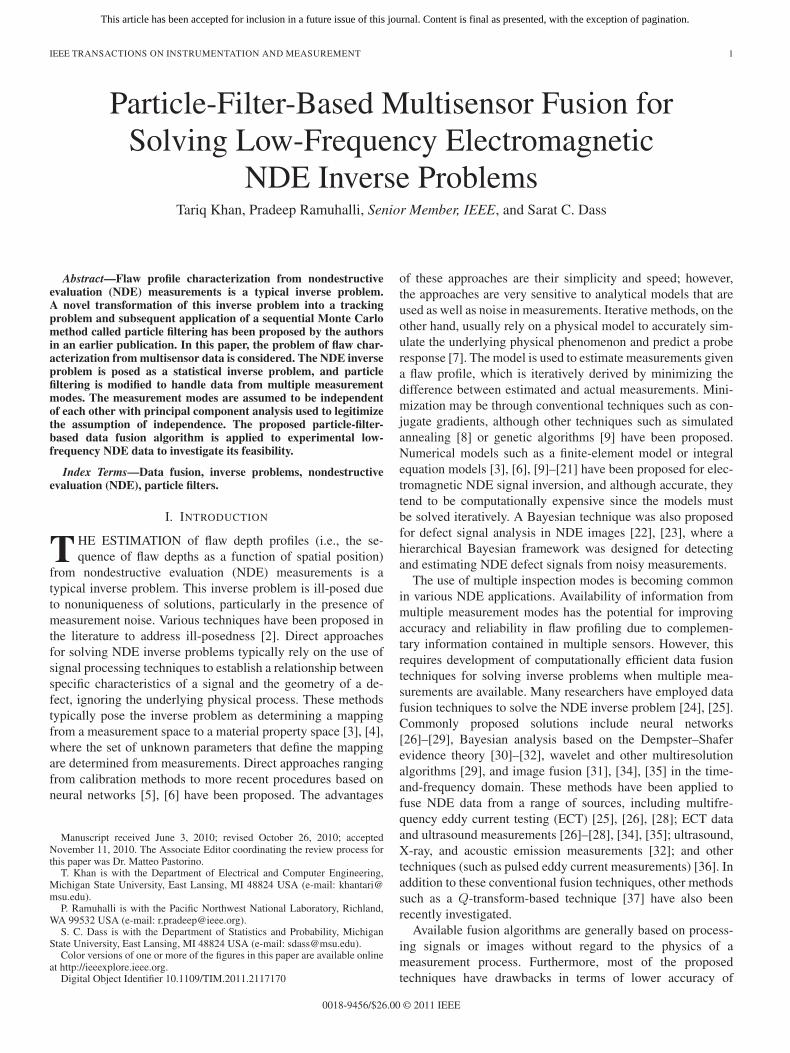
Fig. 1. NDE inverse problem for 1-D flaw profile reconstruction (assumingL = 0).

is equivalent to estimating flaw depths along the length ofa specimen (where the depth along the width dimension isassumed to be invariant). In this case, the length of the specimenis divided into K locations. The 3-D problem is equivalentto estimating flaw depths at each location on a specimensurface; therefore, the surface of the specimen is divided intoK discrete locations. In each case, flaw depth is unknown ateach discretized location. Examples of the formulation for 2-D(cracklike) and 3-D (volumetric flaws such as corrosion, wear,or wall thickness loss) profiling are shown in Figs. 1 and 2,


KHAN et al.: MULTISENSOR FUSION FOR SOLVING ELECTROMAGNETIC NDE INVERSE PROBLEMS 3

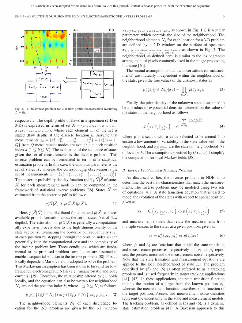
Fig. 2. NDE inverse problem for 2-D flaw profile reconstruction (assumingL = 0).

respectively. The depth profile of flaws in a specimen (2-D or3-D) is expressed in terms of set �X = {x1, x2, . . . , xk−1, xk,xk+1, . . . , xK−1, xK}, where each element xk of the set isstated (flaw depth) at the discrete location k. Assume thatmeasurements z̄k = {z1

k, z2k, . . . , zq

k, . . . , zQk } = {zq

k|q = 1 :Q} from Q measurement modes are available at each positionindex k (1 ≤ k ≤ K). The evaluation of the sequence of statesgiven the set of measurements is the inverse problem. Thisinverse problem can be formulated in terms of a statisticalestimation problem. In this case, the unknown parameter is theset of states �X , whereas the corresponding observation is theset of measurements �Z = {z1

1 , z21 , . . . zQ

1 , z12 , . . . zq

k, . . . zQK}.

The posterior probability density function (pdf) p �X|�Z of states�X for each measurement mode q can be computed in theframework of statistical inverse problems [38]. States �X areestimated from the posterior pdf as follows:

p( �X|�Z) ∝ p(�Z| �X)p( �X). (1)

Here, p(�Z| �X) is the likelihood function, and p( �X) capturesavailable prior information about the set of states (set of flawdepths). The estimation of p(�Z| �X) is generally a computation-ally expensive process due to the high dimensionality of thestate vector �X . Evaluating the posterior pdf sequentially (i.e.,at each position by stepping through the position index k) canpotentially keep the computational cost and the complexity ofthe inverse problem low. Three conditions, which are funda-mental to the proposed problem formulation, are assumed toenable a sequential solution to the inverse problem [38]. First, alocally dependent Markov field is adopted to solve the problem.This Markovian assumption has been shown to be valid for low-frequency electromagnetic NDE (e.g., magnetostatic and eddycurrents) [39]. Therefore, the relationship offered by (1) holdslocally, and the equation can also be written for neighborhoodNk around the position index k, where 1 ≤ k ≤ K, as follows:

p (xk|{z̄j |j ∈ Nk}) ∝ p ({z̄j |j ∈ Nk}|xk) p(xk). (2)

The neighborhood elements Nk of each discretized lo-cation for the 2-D problem are given by the 1-D window

xk−(2L+1):k−1, k+1:k+(2L+1), as shown in Fig. 1 L is a scalarparameter, which controls the size of the neighborhood. Theneighborhood elements Nk for each location for a 3-D problemare defined by a 2-D window on the surface of specimenxp, q| p=m−(2L+1):m−1, m+1:m+(2L+1),

q=n−(2L+1):n−1, n+1:n+(2L+1), as shown in Fig. 2. The

neighborhood, as defined here, is similar to the lexicographicarrangement of pixels commonly used in the image processingliterature [40].

The second assumption is that the observations (or measure-ments) are mutually independent within the neighborhood ofthe state, given the true values of the unknown states as

p ({z̄j |j ∈ Nk}|xk) =∏

j∈Nk

p(z̄j |xj). (3)

Finally, the prior density of the unknown state is assumed tobe a product of exponential densities centered on the value ofthe states in the neighborhood as follows:

p(xk|xj | j∈Nk

j �=k

)= e

−∑

j∈Nk

‖xj−xk‖p

p

(4)

where p is a scalar, with a value selected to be around 1 toensure a low amount of variability in the state value within theneighborhood, and xj | j∈Nk

j �=k

are the states in neighborhood Nk

of location k. The assumptions specified by (3) and (4) simplifythe computation for local Markov fields [38].

B. Inverse Problem as a Tracking Problem

As discussed earlier, the inverse problem in NDE is todetermine the best flaw characteristics that match the measure-ments. The inverse problem may be modeled using two setsof equations [41]: A state transition equation that is used tomodel the evolution of the states with respect to spatial position,given as

xk = fk

(xj | j∈Nk

j �=k

, νk

)⇔ p

(xk|xj | j∈Nk

j �=k

)(5)

and measurement models that relate the measurements frommultiple sensors to the states at a given position, given as

zk = hqk (xk, μq

k) ⇔ p(zk|xk) (6)

where fk and hqk are functions that model the state transition

and measurement processes, respectively, and νk and μqk repre-

sent the process noise and the measurement noise, respectively.Note that the state transition and measurement equations areapplied to the local neighborhood of state xk. The problemdescribed by (5) and (6) is often referred to as a trackingproblem and is used frequently in target tracking applications[41], [42]. In these applications, the state transition functionmodels the motion of a target from the known position xj ,whereas the measurement function describes some function ofthe target position. Process and measurement noise densitiesrepresent the uncertainty in the state and measurement models.The tracking problem, as defined in (5) and (6), is a dynamicstate estimation problem [41]. A Bayesian approach to this



problem is to construct a posterior pdf of the state, based onthe sequence of measurements.

The problem described by (5) and (6) can be shown tobe equivalent to the statistical inverse problem defined by (1)using the following arguments. The state transition function(when taken with the associated process noise distribution) isequivalent to the local prior pdf used in the statistical inverseproblem. Similarly, the measurement function is equivalent tothe local likelihood pdf in the statistical inverse problem when alocally independent Markov field is assumed (see Section II-A).The equivalence of the tracking problem to statistical prob-abilities is also shown in (5) and (6). The advantage of thisequivalence is the potential applicability of solution techniquesfor tracking problems to solve the NDE inverse problem. Notealso that the formulation of the inverse problem as the statisticalinverse problem (1) or, equivalently, a tracking problem, asin (5) and (6), implicitly assumes that the NDE measurementprocess is a localized process; i.e., the measurement at theparticular location k is only affected by the state of the samplein a neighborhood of k. As aforementioned, the Markovianassumption is valid for low-frequency electromagnetic NDE(magnetostatic and eddy current NDE) [40], provided that theneighborhood is selected appropriately.

III. APPLICATION OF PARTICLE FILTERS TO SOLVE NDEINVERSE PROBLEMS USING MULTIPLE-MODE

MEASUREMENT DATA

A. Solutions to the Tracking Problem

Kalman filtering [41] provides an optimal solution to thetracking problem if the following two conditions are met.

1) The function that relates the states in a neighborhood (i.e.,the state transition function) and the function that relatesthe state to measurement (i.e., the measurement function)are linear.

2) The likelihood and prior pdfs are Gaussian.

In general, for the NDE inverse problem, these functions canbe nonlinear, and the pdfs can be non-Gaussian (multimodal).Therefore, the Kalman filter cannot provide an optimal solution,and suboptimal algorithms may be necessary to evaluate flawdepth. Therefore, a more generalized filtering technique isrequired to solve this inverse problem. Particle filters offer sucha generalized filtering technique.

B. Theory of Particle Filters

Particle filters are sequential Monte Carlo methods basedon point-mass (or “particle”) representations of probabilitydensities that can be applied to any state-space model and thatgeneralize traditional Kalman filtering methods [41], [42]. Inthis approach to a dynamic state estimation, the posterior pdfof the state is constructed based on all available information,including the set of received measurements. A brief descriptionof the particle filter algorithm is provided next. To simplifythe discussion, we assume that measurements zk = {zq

k|q =1} ≡ zk from a single-measurement mode (i.e., Q = 1) areavailable. This assumption will be relaxed in the next section,

where we extend the particle filtering framework to incorporatemultimodal measurements.

With the assumption of a single-measurement mode (andtemporarily simplifying the notation by dropping superscriptq), the pdf of state xk conditioned on all measurements up to(and including zk) p(xk, z1:k) may be obtained recursively intwo stages: prediction and update stages. The prediction stageuses the system model to predict the pdf forward from onemeasurement location to the next. Suppose that the required pdfp(xk|z1:k−1) at location k − 1 is available. The prediction stageinvolves using the system model to obtain the prediction densityof the state at k via the Chapman–Kolmogorov equation [41] asfollows:

p(xk|z1:k−1) =∫

p(xk|xk−1)p(xk−1|z1:k−1)dxk−1. (7)

If we consider a Markov process of order 1, thenp(xk|xk−1, z1:k−1) = p(xk|xk−1). Since the state is usuallysubject to unknown disturbances (modeled as random noise),the prediction step generally translates, deforms, and otherwisedistorts the pdf. The update operation uses the latest mea-surement to modify the prediction pdf. This is achieved usingBayes’ theorem as follows:

p(xk|zk) = p(xk|zk, z1:k−1)

=p(zk|xk, z1:k−1)p(xk|z1:k−1)

p(zk|z1:k−1)

=p(zk|xk)p(xk|z1:k−1)

p(zk|z1:k−1)(8)

where the normalizing constant is given by

p(zk|z1:k−1) =∫

p(zk| �X)p( �X|z1:k−1)dxk. (9)

In order to apply particle filtering, the desired posterior pdf isrepresented in terms of samples and associated weights at eachlocation. In order to develop the details of the algorithm, let{xi

k, wik}|1:Ns

denote a random measure that characterizes theposterior pdf at location k. xi

k is the set of support points withassociated weights wi

k, and i = 1 : Ns is the total number ofsamples used. The weights are normalized such that

∑Ns

i=1 wik.

Then, posterior density at k can be approximated as [41]

p(xk|zk) ≈Ns∑i=1

wikδ

(xk − xi

k

). (10)

Normalized weights are chosen using the principle of impor-tance sampling [41]. According to this principle, suppose thatp(x) ∝ π(x) is a probability density from which it is difficult todraw samples but for which π(x) can be evaluated, and samplescan be drawn from π(x). In addition, let xi be the samplesthat are easily generated from proposal q(.) called importancedensity. Then, a weighted approximation to density p(x) isgiven by

p(x) ≈Ns∑i=1

wiδ(x − xi) (11)



where wi ∝ (π(xi)/q(xi)) is the normalized weight of theith particle. Therefore, if samples xi

k were drawn from theimportance density q(x1:k|z1:k), the weights are given by [41]

wik ∝

p(xi

1:k|z1:k

)q(xi

1:k|z1:k

) . (12)

With the reception of measurement zk at position k, we wish toapproximate p(x1:k|z1:k) with a new set of samples. Given theset of weights wk−1 at position k − 1, the weights at position kmay be computed recursively using the weight update equationderived from the principle of importance sampling as

wik ∝ wi

k−1

p(zk|xi

k

)p

(xi

k|xik−1

)q(xi

k|xik−1, zk

) . (13)

The most commonly used variant of a particle filter, the sam-pling importance resampling (SIR) algorithm [42], is used inthis paper. The importance density in the SIR algorithm ischosen as the transition prior to

q(xi

k|xik−1, zk

)= p

(xi

k|xik−1

). (14)

Therefore, from (12) and (13), the following is derived:

wik ∝ wi

k−1p(zk|xi

k

). (15)

We can also write (15) as

wik ∝ p

(zk|xi

k

). (16)

C. Particle Filtering for Multisensor Data Fusion

When multiple measurement modes are available, likelihoodpdfs corresponding to each measurement mode need to beconsidered in weight assignment to the sample. Assume thatwi, q

k is the weight of the sample i at the position index kassigned by the individual measurement mode q. For every sam-ple at each position index, Q weights are therefore computedusing the respective likelihood pdfs. The likelihood functioncorresponding to the qth measurement mode is given by (16)and the following:

wi, qk ∝ p

(zqk|xi

k

). (17)

If the measurement processes are assumed to be indepen-dent, then the joint likelihood due to measurement modesq = 1, 2, . . . , Q is the product of likelihood for the individualmeasurement mode, given by

p(zk|xi

k

)= p

(z1k|xi

k

), p

(z2k|xi

k

), . . . , p

(zQk |xi

k

). (18)

Therefore, from (17) and (18), we get the following:

wik ∝ p

(z1k|xi

k

).p

(z2k|xi

k

). . . p

(zQk |xi

k

). (19)

Using (16) and (19), the final weight assigned to sample i atposition index k is as follows:

wik ∝ wi,1

k , wi,2k , . . . , wi, Q

k . (20)

As aforementioned, it is assumed that the measure-ment processes are independent. However, the measurementprocesses may be correlated, and the assumption of indepen-dence is not valid in that case. In order to make the assumptionof independence more legitimate, the PCA technique is appliedto data from different measurement modes. PCA [43] is math-ematically defined as an orthogonal linear transformation thattransforms the data to a new coordinate system. PCA can alsobe applied to data from multiple measurement modes. At eachposition index k, measurements z1:Q

j |j∈Nkwithin its neigh-

borhood from all measurement modes (1 : Q) are considered.These multidimensional data are now the input of the PCAtechnique. The following steps are carried out to evaluate theprincipal components.

Step 1: The multisensor measurements z1:Qj |j∈Nk

are storedas vector ςq|q=1:Q, where each measurement mode is as-sumed to be one component of the vector.

Step 2: The data vector is adjusted by subtracting out its meangiven by:

ςq = ςq − mean(ςq). (21)

Step 3: The adjusted data vectors are arranged as rows ofa matrix. This newly formed matrix will be called the“adjusted data matrix,” given as

ς = [ς1, ς2, . . . , ςQ]. (22)

Step 4: The covariance matrix of the “adjusted data matrix” iscomputed as follows:

σq = cov(ςq). (23)

Step 5: Eigenvectors λq of the covariance matrix are thenevaluated as follows:

λq = eig(σq). (24)

Step 6: The computed eigenvectors are arranged as rows of anew matrix. This newly formed matrix will be referred toas the ”feature matrix” as follows:

λ = [λ1, λ2, . . . , λQ]. (25)

Step 7: Finally, the “feature matrix” is multiplied by the “ad-justed data matrix”

ψ = λς. (26)

The rows of the resultant matrix ψ are the principal (uncorre-lated) components in the data as follows:

ψ = [ψ1, ψ2, . . . , ψQ]. (27)

The resultant components ψq are uncorrelated to each other.Therefore, the output of the PCA technique is a set of indepen-dent (uncorrelated) data of Q dimensions. These independentcomponents are then treated as the data from separate measure-ment modes.



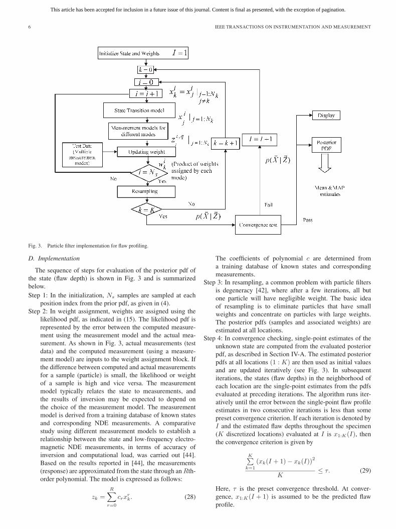
Fig. 3. Particle filter implementation for flaw profiling.

D. Implementation

The sequence of steps for evaluation of the posterior pdf ofthe state (flaw depth) is shown in Fig. 3 and is summarizedbelow.Step 1: In the initialization, Ns samples are sampled at each

position index from the prior pdf, as given in (4).Step 2: In weight assignment, weights are assigned using the

likelihood pdf, as indicated in (15). The likelihood pdf isrepresented by the error between the computed measure-ment using the measurement model and the actual mea-surement. As shown in Fig. 3, actual measurements (testdata) and the computed measurement (using a measure-ment model) are inputs to the weight assignment block. Ifthe difference between computed and actual measurementsfor a sample (particle) is small, the likelihood or weightof a sample is high and vice versa. The measurementmodel typically relates the state to measurements, andthe results of inversion may be expected to depend onthe choice of the measurement model. The measurementmodel is derived from a training database of known statesand corresponding NDE measurements. A comparativestudy using different measurement models to establish arelationship between the state and low-frequency electro-magnetic NDE measurements, in terms of accuracy ofinversion and computational load, was carried out [44].Based on the results reported in [44], the measurements(response) are approximated from the state through an Rth-order polynomial. The model is expressed as follows:

zk =R∑

r=0

crxrk. (28)

The coefficients of polynomial c are determined froma training database of known states and correspondingmeasurements.

Step 3: In resampling, a common problem with particle filtersis degeneracy [42], where after a few iterations, all butone particle will have negligible weight. The basic ideaof resampling is to eliminate particles that have smallweights and concentrate on particles with large weights.The posterior pdfs (samples and associated weights) areestimated at all locations.

Step 4: In convergence checking, single-point estimates of theunknown state are computed from the evaluated posteriorpdf, as described in Section IV-A. The estimated posteriorpdfs at all locations (1 : K) are then used as initial valuesand are updated iteratively (see Fig. 3). In subsequentiterations, the states (flaw depths) in the neighborhood ofeach location are the single-point estimates from the pdfsevaluated at preceding iterations. The algorithm runs iter-atively until the error between the single-point flaw profileestimates in two consecutive iterations is less than somepreset convergence criterion. If each iteration is denoted byI and the estimated flaw depths throughout the specimen(K discretized locations) evaluated at I is x1:K(I), thenthe convergence criterion is given by

K∑k=1

(xk(I + 1) − xk(I))2

K≤ τ. (29)

Here, τ is the preset convergence threshold. At conver-gence, x1:K(I + 1) is assumed to be the predicted flawprofile.



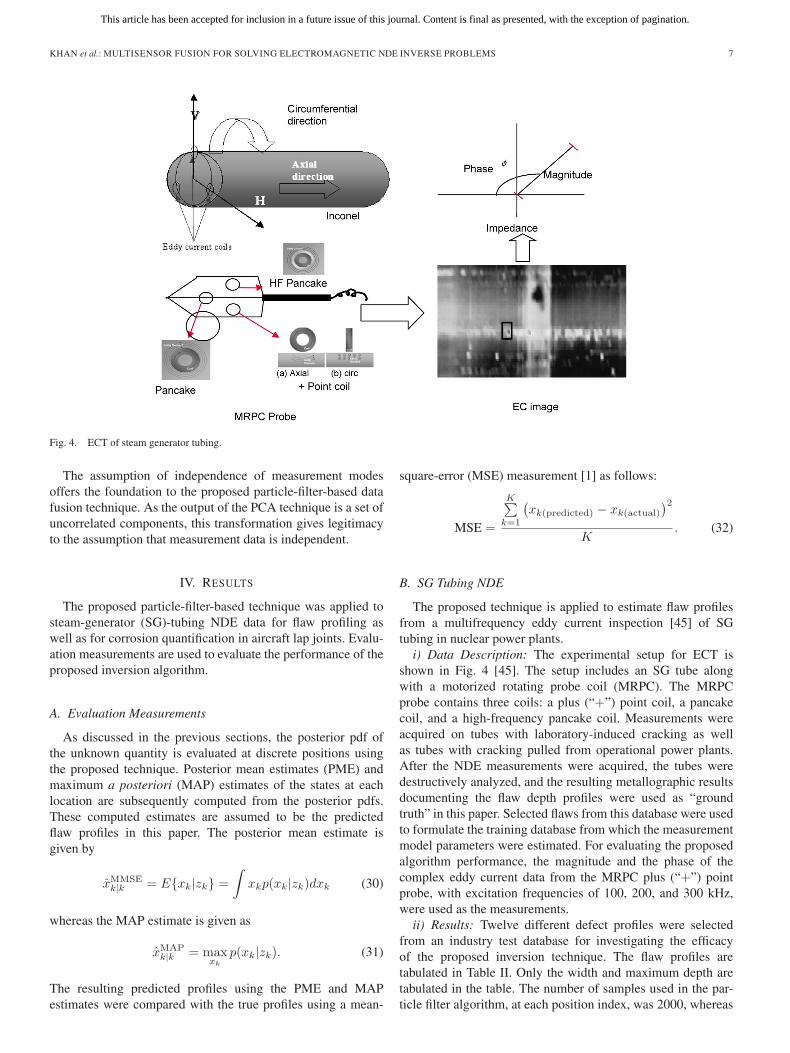
Fig. 4. ECT of steam generator tubing.

The assumption of independence of measurement modesoffers the foundation to the proposed particle-filter-based datafusion technique. As the output of the PCA technique is a set ofuncorrelated components, this transformation gives legitimacyto the assumption that measurement data is independent.

IV. RESULTS

The proposed particle-filter-based technique was applied tosteam-generator (SG)-tubing NDE data for flaw profiling aswell as for corrosion quantification in aircraft lap joints. Evalu-ation measurements are used to evaluate the performance of theproposed inversion algorithm.

A. Evaluation Measurements

As discussed in the previous sections, the posterior pdf ofthe unknown quantity is evaluated at discrete positions usingthe proposed technique. Posterior mean estimates (PME) andmaximum a posteriori (MAP) estimates of the states at eachlocation are subsequently computed from the posterior pdfs.These computed estimates are assumed to be the predictedflaw profiles in this paper. The posterior mean estimate isgiven by

x̂MMSEk|k = E{xk|zk} =

∫xkp(xk|zk)dxk (30)

whereas the MAP estimate is given as

x̂MAPk|k = max

xk

p(xk|zk). (31)

The resulting predicted profiles using the PME and MAPestimates were compared with the true profiles using a mean-

square-error (MSE) measurement [1] as follows:

MSE =

K∑k=1

(xk(predicted) − xk(actual)

)2

K. (32)

B. SG Tubing NDE

The proposed technique is applied to estimate flaw profilesfrom a multifrequency eddy current inspection [45] of SGtubing in nuclear power plants.

i) Data Description: The experimental setup for ECT isshown in Fig. 4 [45]. The setup includes an SG tube alongwith a motorized rotating probe coil (MRPC). The MRPCprobe contains three coils: a plus (“+”) point coil, a pancakecoil, and a high-frequency pancake coil. Measurements wereacquired on tubes with laboratory-induced cracking as wellas tubes with cracking pulled from operational power plants.After the NDE measurements were acquired, the tubes weredestructively analyzed, and the resulting metallographic resultsdocumenting the flaw depth profiles were used as “groundtruth” in this paper. Selected flaws from this database were usedto formulate the training database from which the measurementmodel parameters were estimated. For evaluating the proposedalgorithm performance, the magnitude and the phase of thecomplex eddy current data from the MRPC plus (“+”) pointprobe, with excitation frequencies of 100, 200, and 300 kHz,were used as the measurements.

ii) Results: Twelve different defect profiles were selectedfrom an industry test database for investigating the efficacyof the proposed inversion technique. The flaw profiles aretabulated in Table II. Only the width and maximum depth aretabulated in the table. The number of samples used in the par-ticle filter algorithm, at each position index, was 2000, whereas



TABLE IIEXPERIMENTAL FLAW PROFILES

Fig. 5. Proposed inversion technique. (a) Phase measurement. (b) Magnitude measurement. (c)Three-dimensional and (d) top views of the posterior pdf.(e) Computed estimates.

a third-order polynomial measurement model was used. Threedifferent values of parameter L (0, 1, and 2) were used. Theconvergence threshold used in this paper was τ = 10−3. Fig. 5

shows the inversion results using data fusion of magnitude andphase measurement at 300 kHz for a flaw with a width of 7 mmand a maximum depth of 100% of tube wall thickness. Fig. 5(a)



Fig. 6. MSE between the PME of the posterior pdf and the true profilesversus the state vector length parameter L at different measurement modes forexperimental data.

Fig. 7. Mean and standard deviations of the MSE (between the PME and thetrue profile) versus L at different measurement modes.

and (b) shows phase and amplitude measurements, respectively.Fig. 5(c) and (d) shows the top and 3-D views of the com-puted posterior pdfs, respectively. Fig. 5(e) shows the computedestimates.

Fig. 6 presents a summary of the MSE between the PME andtrue flaw profiles for the 12 flaws, using different measurementmodes and the state vector length parameter L = 0, 1, 2. TheMSE between the PME and the true flaw profile using mea-surement data at three individual frequencies (100, 200, and300 kHz) are shown. The MSE between the PME and trueprofiles using data fusion of measurement modes without PCAand with PCA are shown in Fig. 6. The average and standarddeviation of the MSE for each measurement mode are shown inFig. 7.

C. Corrosion Quantification in Aircraft Lap Joints

i) Data Description: Quantification of the loss of platethickness due to corrosion on an aircraft skin is presentedas a test case for 3-D flaw profile construction. The NDE

Fig. 8. Aircraft lap joint specimen.

measurement data was acquired from a 30-year-old service-retired Boeing 727 aircraft, as shown in Fig. 8. Two specimens(C and D), each consisting of a two-layer aluminum 2024-T3lap joint cut out from below the cargo floor, were inspected.The thickness of each layer of the lap joint is 0.045 in (1.143mm). The specimens were disassembled and cleaned of allcorrosion products after the inspection. X-ray mappings werethen acquired to assess the true plate thickness. The inversionresults were compared with the true thickness to determinethe efficacy of the technique. Measurements from multiple-frequency eddy current modes (5.5, 17, and 30 kHz) were usedin the inversion. The number of samples Ns in the particle filterwas 2000. The resulting predicted profiles using PMEs and theMAP estimates are compared with the true profiles using a rootMSE measurement [46].

ii) Results: The inversion result evaluated using a single-measurement mode and fusing multiple measurement modesfor specimen C is shown in Fig. 9. Results for specimens Cand D are tabulated in Table III. Results indicate improvementin inversion accuracy when data fusion is used.

D. Discussion

Flaw depth profiling results from eddy current measurementsindicate that the proposed particle filter approach is capable ofproducing reasonably accurate results even in the presence ofnoise. In particular, results on experimental data validate the ro-bustness of the proposed approach and indicate the feasibility ofthe proposed inversion technique. The use of data fusion is alsoseen to reduce the error in the reconstruction when compared toflaw profiles obtained using a single-measurement mode. Theuse of PCA further increases the accuracy of inversion. Notethat in all cases, the flaw profile reconstruction processes wereobtained using the particle-filtering algorithm. Comparisonwith other contemporary techniques reported in the literature[46] indicates that the inversion results using particle filtering(with or without data fusion) are either comparable to or betterthan the results obtained using these other techniques. Theresults also indicate that using a large neighborhood improvesthe inversion results. Note that the depth variation in real flawscan be abrupt, and flaw depth does not remain constant forlong spans. This fact is a challenge for the proposed inversiontechnique. The use of a larger neighborhood (large value ofL) appears to smooth out the variations in the flaw profilesand improves inversion accuracy. However, increasing the sizeof the neighborhood increases the computational cost. Forinstance, increasing L from 0 to 2 increases the computationalload by a factor of 5 [47].



Fig. 9. Inversion results of specimen C (data fusion). (a) and (e) True profile. (b)–(d) and (f) Predicted profiles using ET data at 5.5, 17, 30 kHz and data fusion.

TABLE IIIINVERSION RESULTS FOR SECTIONS C AND D

V. CONCLUSION & FUTURE WORK

A sequential Monte-Carlo-based data fusion technique wasproposed for solving inverse problems. Results on multipledatabases indicate the efficacy of the proposed inversion tech-

nique. The proposed data fusion technique is based on theassumption that measurement processes are statistically in-dependent processes, and the use of PCA was proposed tofurther legitimatize the assumption. The results indicate that the



inversion results improve when data from multiple measure-ment modes are fused. A further improvement is observed in theinversion results when PCA is used prior to data fusion. Futurework will focus on investigation of alternative preprocessingapproaches when the assumption of independence is not valid.Application of the proposed technique on other types of datasets is another focus area for future work. These data setsinclude X-ray tomography and ultrasonic data.

REFERENCES

[1] T. Khan and P. Ramuhalli, “A recursive Bayesian estimation method forsolving electromagnetic NDE inverse problems,” IEEE Trans. Magn.,vol. 44, no. 7, pp. 1845–1855, Jul. 2008.

[2] A. Tarantola, Inverse Problem Theory: Methods for Model ParameterEstimation. Amsterdam, The Netherlands: Elsevier, 1987.

[3] L. Udpa and S. Udpa, “Neural application of signal processing and patternrecognition techniques to inverse problems in NDE,” Int. J. Appl. Electro-magn. Mech., vol. 8, pp. 99–117, 1997.

[4] H. Sohn, C. Farrar, F. Hemez, D. Shunk, D. Stinemates, andB. Nadler, “A review of structural health monitoring literature: 1996–2001,” Los Alamos Nat. Lab., Los Alamos, NM, Tech. Rep. LA-13976-MS, 2003.

[5] P. Ramuhalli, L. Udpa, and S. Udpa, “Electromagnetic NDE signalinversion using function approximation neural networks,” IEEE Trans.Magn., vol. 38, no. 6, pp. 3633–3642, Nov. 2002.

[6] P. Ramuhalli, L. Udpa, and S. Udpa, “Neural network algorithm forelectromagnetic NDE signal inversion,” in Electromagnetic Nondestruc-tive Evaluation V . Amsterdam, The Netherlands: IOS Press, 2001,pp. 121–128.

[7] M. Yan, M. Afzal, S. Udpa, S. Mandayam, Y. Sun, L. Udpa,and P. Sacks, “Iterative algorithms for electromagnetic NDE signalinversion,” in ENDE (II), R. Albanese, G. Rubinacci, T. Takagi, andS. S. Udpa, Eds. Amsterdam, The Netherlands: IOS Press, 1998,ser. Studies in Applied Electromagnetic and Mechanics, pp. 287–296.

[8] S. Kirkpatrick, C. D. Gelatt, and M. P. Vecchi, “Optimization bysimulated annealing,” Science, vol. 220, no. 4598, pp. 671–680, May 13,1983.

[9] R. L. Haupt, “An introduction to genetic algorithms for electromag-netics,” IEEE Trans. Antennas Propag., vol. 37, no. 2, pp. 7–15,Apr. 1995.

[10] S. Hoole, S. Subramanian, R. Saldanha, and J. Coulomb, “Inverse problemmethodology and finite elements in the identification of cracks, sources,materials, and their geometry in inaccessible locations,” IEEE Trans.Magn., vol. 27, no. 3, pp. 3433–3443, May 1991.

[11] K. Arunachalam, V. Melapudi, E. Rothwell, L. Udpa, and S. Udpa,“Microwave NDE for reinforced concrete,” in Proc. Quant. Nondestruct.Eval., 2005, pp. 455–460.

[12] Z. Zeng, C. Lu, B. Shanker, and L. Udpa, “Element-free Galerkinmethod in modeling microwave inspection of civil structures,” in Proc.12th Biennial IEEE Conf. Electromagn. Field Comput., 2006, vol. 27,p. 268.

[13] K. Arunachalam, “Investigation of a deformable mirror microwaveimaging and therapy technique for breast cancer,” Ph.D. dissertation,Michigan State Univ., East Lansing, MI, 2006.

[14] Y. Kim, L. Jofre, F. D. Flaviis, and M. Q. Feng, “Microwave reflectiontomographic array for damage detection of civil structures,” IEEE Trans.Antennas Propag., vol. 51, no. 11, pp. 3022–3032, Nov. 2003.

[15] Y. Li, G. Liu, B. Shanker, Y. Sun, P. Sacks, L. Udpa, and S. S. Udpa, “Anadjoint equation based method for 3D eddy current NDE signal inver-sion,” in Electromagnetic Nondestructive Evaluation (V). Amsterdam,The Netherlands: IOS Press, 2001, pp. 89–96.

[16] Y. Li, L. Udpa, and S. Udpa, “Three-dimensional defect reconstructionfrom eddy-current NDE signals using a genetic local search algorithm,”IEEE Trans. Magn., vol. 27, no. 2, pp. 410–417, Mar. 2004.

[17] V. Monebhurrun, B. Duchene, and D. Lesselier, “3D inversion of eddycurrent data for nondestructive evaluation of steam generator tubes,”Inverse Probl., vol. 14, no. 3, pp. 707–724, Jun. 1998.

[18] M. Morozov, G. Rubinnaci, A. Tamburrino, and S. Ventre, “Numericalmodels of volumetric insulating cracks in eddy-current testing with ex-perimental validation,” IEEE Trans. Magn., vol. 42, no. 5, pp. 1568–1576,May 2006.

[19] S. Balasubramaniam, B. Shanker, and L. Udpa, “A fast integral equa-tion based scheme for computing magnetostatic fields and its application

to NDE problems,” in Proc. Quant. Nondestruct. Eval., 2001, vol. 20,pp. 331–337.

[20] R. Schifini and A. C. Bruno, “Experimental verification of a finite elementmodel used in a magnetic flux leakage inverse problem,” J. Phys. D, Appl.Phys., vol. 38, no. 12, pp. 1875–1880, Jun. 2005.

[21] S. Caorsi, G. L. Gragnani, S. Medicina, M. Pastorino, and G. Zunino,“Microwave imaging based on a Markov random field model,” IEEETrans. Antennas Propag., vol. 42, no. 2, pp. 293–303, Mar. 1994.

[22] A. Dogandzic, “Bayesian NDE defect signal analysis,” IEEE Trans.Signal Process., vol. 55, no. 1, pp. 372–378, Jan. 2007.

[23] A. Dogandzic and B. Zhang, “Markov chain Monte Carlo defectidentification in NDE images,” in Review of Progress in QuantitativeNondestructive. Melville, NY: AIP, 2007.

[24] Z. Liu, D. S. Forsyth, J. P. Komorowski, K. Hanasaki, and T. Kirubarajan,“Survey: State of the art in NDE data fusion techniques,” IEEE Trans.Instrum. Meas., vol. 56, no. 6, pp. 2435–2451, Dec. 2007.

[25] X. E. Gross, NDT Data Fusion. Boston, MA: Butterworth-Heinemann,1997.

[26] J. Yim, S. S. Udpa, M. Mina, and L. Udpa, “Optimum filter based tech-niques for data fusion,” in Review of Progress in QNDE, D. O. Thompsonand D. E. Chimenti, Eds. New York: Plenum, 1996, pp. 773–780.

[27] J. Yim, S. S. Udpa, L. Udpa, and W. Lord, “Neural network approachesto data fusion,” in Review of Progress in QNDE, D. O. Thomson andD. E. Chimenti, Eds. New York: Plenum, 1995, pp. 819–826.

[28] G. Simone and F. C. Morabito, “NDT image fusion using eddy current andultrasonic data,” COMPEL-Int. J. Comput. Math. Elect. Electron. Eng.,vol. 20, no. 3, pp. 857–868, 2001.

[29] J. Dion, M. Kumar, and P. Ramuhalli, “Multi-sensor data fusion forhigh-resolution material characterization,” in Proc. Rev. Prog. QNDE,vol. 894, AIP Conference Proceedings, 2007, pp. 1189–1196.

[30] X. E. Gros, P. Strachan, and D. W. Lowden, “Theory and implementationof NDT data fusion,” Res. Nondestruct. Eval., vol. 6, no. 4, pp. 227–236,Dec. 1995.

[31] X. E. Gros, Z. Liu, and K. Hanasaki, “Experimenting with pixel levelNDT data fusion techniques,” IEEE Trans. Instrum. Meas., vol. 49, no. 5,pp. 1083–1090, Oct. 2000.

[32] V. Kaftandjian and N. Francois, “Use of data fusion methods to improvereliability of inspection: Synthesis of the work done in the frame of aEuropean thematic network,” in Proc. 8th ECNDT , Barcelona, Spain,Jun. 2002, vol. 8, no. 2, NDT. net.

[33] Z. Liu, K. Tsukada, and K. Hansaki, “One-dimensional eddy cur-rent multi-frequency data fusion: A multi-resolution analysis approach,”Insight, vol. 40, no. 4, pp. 286–289, Apr. 1998.

[34] Y. W. Song and S. S. Udpa, “A new morphological algorithm for fusingultrasonic and eddy current images,” in Proc. IEEE Ultrason. Symp.,1996, pp. 649–652.

[35] Z. Liu, X. E. Gros, K. Tsukada, and K. Hanasaki, “3D visualization ofultrasonic inspection data by using AVS,” in Proc. 5th Far-East Conf.Nondestruct. Test., Kenting, Taiwan, Nov. 1999, pp. 549–554.

[36] D. S. Forsyth and J. P. Komorowski, “The role of data fusion in NDE foraging aircraft,” Proc. SPIE, vol. 3994, pp. 47–58, 2000.

[37] K. Sun, S. S. Udpa, L. Udpa, T. Xue, and W. Lord, “Registrationissues in the fusion of eddy current and ultrasonic NDE data usingQ-transforms,” in Review of Progress in QNDE, D. O. Thompson andD. E. Chimenti, Eds. New York: Plenum, 1996, pp. 813–820.

[38] G. Givens and J. Hoeting, Computational Statistics. Hoboken, NJ:Wiley, 2005, ser. Wiley Series in Probability and Statistics.

[39] A. Tamburrino, “A communication theory approach for electromagneticinverse problems,” IEEE Trans. Magn., vol. 36, no. 4, pp. 1136–1139,Jul. 2000.

[40] N. Alves, “Ising model Monte Carlo simulations: Density of states andmass gap,” Phys. Rev. B, Condens. Matter, vol. 41, no. 1, pp. 383–394,Jan. 1990.

[41] B. Ristic, S. Arulampalam, and N. Gordon, Beyond the Kalman Filter.London, U.K.: Artech House, 2004.

[42] S. Arulampalam, S. Maskell, N. Gordon, and T. Clapp, “A tutorial onparticle filters for on-line non-linear/non-Gaussian Bayesian tracking,”IEEE Trans. Signal Process., vol. 50, no. 2, pp. 174–188, Feb. 2002.

[43] I. T. Jolliffe, Principal Component Analysis. New York: Springer-Verlag, 2002.

[44] T. Khan and P. Ramuhalli, “Sequential Monte Carlo methods forelectromagnetic NDE inverse problems—Evaluation and comparisonof measurement models,” IEEE Trans. Magn., vol. 45, no. 3, pp. 1566–1569, Mar. 2009.

[45] J. R. Bowler, “Review of eddy current inversion with application to non-destructive evaluation,” Int. J. Appl. Electromagn. Mech., vol. 8, pp. 3–16,1997.



[46] Z. Liu, P. Ramuhalli, S. Safizadeh, and D. S. Forsyth, “Combining multi-ple nondestructive inspection images with a generalized additive model,”Meas. Sci. Technol., vol. 19, no. 8, p. 085701, Aug. 2008.

[47] T. Khan, “A sequential Monte Carlo based recursive technique for solvingNDE inverse problems,” Ph.D. dissertation, ECE, MSU, East Lansing,MI, 2009.

Tariq Khan received the Ph.D. degree in electricalengineering from Michigan State University, EastLansing, in 2009.

Currently, he is a Research Associate with theDepartment of Electrical and Computer Engineering,Michigan State University. His primary research in-terests include the development and applications ofsensors and statistical signal processing algorithmsfor nondestructive evaluation applications.

Pradeep Ramuhalli (M’02–SM’08) received theB.Tech. degree from Jawaharlal Nehru Technolog-ical University, Hyderabad, India, in 1995 and theM.S. and Ph.D. degrees in electrical engineeringfrom Iowa State University, Ames, in 1998 and 2002,respectively.

He has previously worked as an Assistant Profes-sor with the Department of Electrical and ComputerEngineering, Michigan State University, East Lans-ing. Since 2009, he is working as a senior researchscientist at Pacific Northwest National Laboratory,

Richland, WA. He has developed novel algorithms based on neural networksand Monte Carlo techniques for solving electromagnetic and acoustic inverseproblems, and physics-based multisensor data fusion of electromagnetic andacoustic data. He has also investigated innovative radio-frequency identificationtag sensors for structural health monitoring. Applications of his research arein life extension of legacy nuclear power plants, safety assessment of next-generation nuclear power plants, noise mitigation, and structural integrityassessment of civil structures. His research interests include the broad areasof integrated system health monitoring and prognostics, inverse problems,multisensor data fusion, numerical methods, and image/signal processing.

Dr. Ramuhalli is a member of the American Nuclear Society, Phi Kappa Phi,and Sigma Xi.

Sarat C. Dass received the M.Sc. and Ph.D. degreesin statistics from Purdue University, West Lafayette,IN, in 1995 and 1998, respectively.

Currently, he is an Associate Professor with theDepartment of Statistics and Probability, MichiganState University, East Lansing. He has developed sta-tistical models and methodology for several impor-tant engineering problems in his collaborations. Hisresearch interests include statistical image process-ing and pattern recognition, shape analysis, spatialstatistics, Bayesian computational methods, founda-

tions of statistics, and nonparametric statistical methods.

ieeetransactions on instrumentation and …sdass/papers/particlefilterieee2011.pdf · digital...

Documents