i&i/ a - nasa · the dynamic analysis of truss structures may require detailed modeling to...
TRANSCRIPT

NASATechnical
Paper2661
1987
I&I/ ANational Aeronauticsand Space Administralion
Scientific and TechnicalInformation Branch
Modeling of Joints forthe Dynamic Analysisof Truss Structures
W. Keith Belvin
Langley Research Center
Hampton, Virginia
https://ntrs.nasa.gov/search.jsp?R=19870011134 2018-05-27T14:13:03+00:00Z


Summary
A method for modeling joints to assess the influence of joints on the dynamic response of truss
structures has been developed. The analytical models, which are based on experimental joint
load-deflection behavior, use springs and dampers to simulate joint behavior. An algorithm for
automatically computing nonlinear coefficients of the analytical models is also presented. The joint
models are incorporated into a nonlinear finite-element program through use of special nonlinear
spring, viscous, and friction elements. Next, the effects of nonlinear joint stiffness, such as dead
band in the joint load-deflection behavior, are studied. Linearization of joint stiffness nonlinearities
is performed to assess the accuracy of linear analysis in predicting nonlinear response. Viscous
and friction damping are then used to show the effects of joint damping on global beam and truss
structure response and equations for predicting the sensitivity of beam deformations to changes in
joint stiffness are derived. In addition, the frequency sensitivity of a truss structure to-random
perturbations in joint stiffness is discussed and results are shown which indicate that average joint
properties may be sufficient for predicting truss response.
Introduction
The increased access to space made possible by the NASA Space Transportation System has
resulted in radically new spacecraft designs. Spacecraft larger than 300 ft in diameter, such as
the hoop-column antenna (ref. l) and the Space Station reference configurations (ref. 2), are being
designed. These spacecraft, shown in figures 1 and 2, make extensive use of truss structures to span
large distances because trusses provide high stiffness with low mass. Many of these spacecraft require
accurate dynamic analysis for prediction of loads, stability, shape control, and pointing accuracy.
The dynamic analysis of truss structures may require detailed modeling to maintain accuracy in the
analysis.
Individual truss members are connected to one another through joints. In most civil engineering
truss structures, joints are typically welded or bolted so that little or no displacement occurs across
the joint relative to the displacement of the members. For this type of joint, analytical modeling
assumes either member-to-member rigid or pinned connections. Truss structures proposed for space
applications have joint designs which permit the erection or deployment of the truss members. Unlike
civil engineering structures, joint designs for space structures have finite tolerances between mating
surfaces which permit the joints to rotate or to be latched. Tolerances result in a region of dead
band where joint motion can occur with near-zero force. Joint dead band is believed to significantly
affect the response of truss structures and may require detailed modeling to include these effects in
the overall, or global, analysis.
Truss structures are often referred to as being "joint dominated" because of the number of joints
and their influence on overall truss response. The joints influence the dynamic response of trusses in
two major ways, first by reducing the effective truss stiffness and second by introducing additional
damping compared with structures for which the members are rigidly connected. To predict the
influence of joints on truss response, detailed characterization of joint properties will likely be
necessary. Several publications describe experimental characterizations of joints and modeling of
jointed structures.
Built-up structures possess a number of mechanisms to dissipate energy resulting from the
mechanical interfaces or joints which join structural components together. References 3 to 7 discuss
a large number of joint tests and analyses to determine the dominant sources of joint damping. At
low frequencies, there is uniform agreement that Coulomb friction mechanisms on a macroscopic
level dissipate the majority of the energy. At higher frequencies, Aubert et al. (ref. 7) have identified
a number of rate-dependent damping mechanisms that. dissipate energy. Examples of rate-dependent
joint damping mechanisms are acoustic radiation, air pumping, viscous damping, and impacting of
surfaces. Only structures with low-frequency oscillations are considered in this study; thus, only
Coulomb friction and viscous damping have been included in the analysis herein.

To obtainanalyticalmodelsof joints, the dampingandthe stiffnessof the joints shouldbemeasuredfromthejoint hardware.Reference8 hasusedclassicload-deflectiontestingto measurejoint stiffuess.Load-deflectiontestingcanalsobeusedto extractdampinginformationby testingat severaldifferentloadingrates.At highfrequencies,the individualload-deflectioncurvesdonotdescriberate-dependentdampingmechanismsadequately.Consequently,theauthorsof references7and9 haveuseda modifiedload-deflectiontechniquecalledforce-statemapping.Force-statemaps,asshownin figure3, areproducedfrom a three-dimensionalplot of the joint responsein whichforce,velocity,anddisplacementaredisplayed.Resultsfromreferences7 and9 indicateforce-statemappingis a viablejoint testmethodevenat relativelyhighfrequencies.Thejoint testmethodusedin this study is load-deflectiontesting. Thismethodwaschosenbecauseonly low-frequencyvibrationsareconsidered.
The majority of existingmethodsfor modelingstructureswith joints usevariationsof thecomponentsynthesismethod.Craigpresentsa goodreviewof state-of-the-artsynthesismethodsin reference10. For rigid connections,the basicmethodspresentedin references11to 15maybeemployed.However,whenthe connectionsareflexible,as is the casein practice,the numberof viablecomponentsynthesismethodsis reduced.Onemethodwhichenablescomponentsto beconnectedthroughflexiblejointsisreferredtoasastiffnesscouplingprocedure(ref.16).Thestiffnesscouplingprocedureallowsnaturalvibrationmodesof componentsto becombinedthroughalinearstiffnessmatrix. Anothermethodhasbeenproposed(refs.17to 20)whichexploitsLagrange'sequationsandLagrangemultiplierstoallowcomponentsto beconnectedthroughnonrigidconstraintrelations.In reference20,ageneralizationof theLagrangemultipliermethodpermitstheanalysisofstructuresconnectedbynonlinearjoints.Forstructureswithonlyafewjoints,thismethodisfeasible.However,for structureswith manyjoints,the Lagrangemultipliermethodrequiresthe solutionofmanyadditionalequations.Thus,componentsynthesismethodsfor systemswith manynonlinearjoints donot appearto beanymoreefficientthan finite-elementanalysismethods.Consequently,thepresentstudyfocusesondevelopinga finite-element-basedanalysisfor detailedjoint modelingbecauseof its generalityandeaseof implemcntation.
Theobjectiveof this studyis to developa systematicprocedurewherebytheinfluenceofjointsontheresponseoftrussstructurescanbequantitativelydetermined.Thisprocedurecanbebrokeninto threeareas:First, joint characteristicsaredeterminedexperimentally.Second,analysesaredevelopedwhichenablejoint-dominatedstructureresponseto be accuratelypredicted. Third,numericalstudiesaremadeof the structureresponse.Severaljoint modelsare developed,andmodelstiffnessanddampingparametersaredeterminedwith analgorithmbasedonoptimizationtechniques.Incorporationof the joint modelsinto globalstructuralanalysisisperformedwith thefinite-clementmethod.Numericalexamplesof the transientresponseof beamandtrussstructureswith joints are thenpresented.The effectsof stiffnessnonlinearitiesandviscousand frictionaldampingmechanismsarealsostudied. Finally,numericalresultsof linearizedjoint modelsarecomparedwith full nonlinearresuIts,andthe sensitivityof globalstructureresponseto variationsin joint propertiesispresented.
Nomenclature
A
B
C
C1
C
E
Ed
cross-sectional area of the beam
viscous damping matrix
magnitude of joint dead band
initial joint dead band position
viscous damping coefficient
Young's modulus of the beam material
energy dissipated by damping
2

F
F f
f
G
I
K
k
ku, kw, k¢
M
77/
N
N_
O
t
u
tu
X
P
¢
¢
03
0.)8_
Superscripts:
a, b, c
Subscripts:
a, b, c, d
J
R
Analysis
force vector
friction damping force
frequency
shear modulus of the beam material
moment of inertia of the beam cross section
stiffness matrix
spring stiffness of the joint
spring stiffness of the joints in the axial, lateral, and rotational displacement
directions
normalized spring stiffness of the joints in the axial, lateral, and rotational
displacement directions (see eqs. (10))
total beam length
mass matrix
nodal mass
vector of friction forces
number of time steps
objective function
time
axial displacement
lateral displacement
total joint displacement
mass density of the beam material
rotational displacement
nodal displacement vector
nodal velocity vector
nodal acceleration vector
circular frequency
circular frequency of simply supported beam
parts of the joint model (see fig. 6)
nodes of the joint elements and of the beam
beam deformations with joints
beam deformations without, joints
Analytical joint models should permit joint damping and stiffness behavior to be simulated, but
should be simple enough so that the model parameters can be identified from test data. The design
of trussstructurejoints canproduceeccentricitiesin the loadtransmissionpathwhichresultincouplingofaxial,bending,torsion,andsheardeformations.Thus,completecharacterizationofjointdampingandstiffnessrequiresa seriesof testswhichcan identifycoefficientsof fully populateddampingand stiffnessmatrices.This task is evenflmher complicatedby the fact that manyofthe joint propertiesarenonlinear,so that linearsuperpositioncannotbe used. Assumptionsintheanalysisarerequiredto permitthe modelparametersto be identifiedthrougha limitedseriesof tests. The presentstudyusesa nonlinearmodelfor the load-deflectionrelationship;however,couplingbetweenaxial,bending,torsion,andsheardeflectionshasbeenneglected.Thissimplifyingassumptionresultsin identificationof only the diagonaltermsof the joint dampingandstiffnessmatrices.
Thejoint modeldevelopmentmethodusedhereinfollowstheflowchartof figure4. Threemajorcomponentsof modeldevelopmentareinvolved.First, choosethe formof thejoint analysismodelto beusedin the globalanalysisof the trussstructure. Second,designand conducta seriesofexperimentsto determinetheload-deflectionbehaviorof thejoint. Thetypeof experimentdependson the formof the chosenanalysismodel.Forexample,if no rate-dependentdampingis modeledin tile analysis,onlystatictestsarerequired.Third, determinecoefficientsof theanalyticalmodelwhichmostcloselyreconstructtheexperimentaljoint behavior.Thisisusuallyaccomplishedthroughminimizationof theerrorbetweenthepredictedandthemeasuredresponse.
Thenext threesectionsdiscussthethreecomponentsofjoint,modeldevelopment.Anextensionof thestandardanelasticmodel(ref. 19)isdescribed,followedbya descriptionofexperimentaltestswhichcanbe usedto characterizejoint behavior.Sampleexperimentaldataarepresentedfroma representativespacetrussjoint, andanalgorithmis usedto reducethe experimentaldata intocoefficientsof the joint analyticalmodel. Numericalresultsfromthe algorithmarepresentedforbothsimulatedandexperimentaldata.Subsequently,thefinite-elementprogramforglobalanalysisof beamandtrussstructuresisdescribed.
Model Selection
Analytical models for truss structure joints should be of a form which can be incorporated into
the global structure analysis. This study uses the finite-element method for the global analysis; thus,
it is only natural that the joint models should be finite elements. Linear springs and linear viscous
dampers are the simplest joint finite elements. As described previously, a number of nonlinear
stiffness and damping mechanisms are present in structural joints. Consequently, nonlinear springs
and dampers have been chosen to model the joint response.
In reference 21, Lazan presented several models which have been used in material stiffness and
damping analysis. The Maxwell model consists of a viscous damper in series with a spring. The
Maxwell model, shown in figure 5, exhibits infinite creep as the frequency of excitation approaches
zero. The Voight model eliminates the creep problem by placing the spring in parallel with the
damper. Unfortunately, the Voight model becomes rigid at high frequencies. An anelastic model of
a Voight unit in series with a spring is also shown in figure 5. This three-parameter model, referredto as the standard anelastic model, exhibits none of the limitations of tile Voight or Maxwell models.
Since joints exhibit material damping characteristics as well as macroscopic Coulomb friction, the
standard anelastie model has been modified as shown in figure .5. The standard anelastic model is
augmented with a friction-spring unit placed in series with the other elements. The resulting model isreferred to herein as the modified standard anelastic (MSA) model. Nonlinear response of the MSA
model can be aqhieved if some or all of the coefficients are allowed to be functions of displacement,
velocity, or load, or any combination of these three. Displacement-dependent coefficients have been
used in this study for the stiffness, friction, and viscous coefficients.
Tile MSA model has four nodes, as indicated in figure 6. For each degree of freedom (DOF) a
different set of coefficients relates the displacement of that degree of freedom to the applied load.
4

The MSA model has three components in series, and the total displacement across the joint is
(Ca -- Cd) = (¢_ -- Cb) + (¢b -- ¢c) + (¢c -- Cd) (1)
where ¢ is the nodal displacement vector. For the planar structures analyzed in this study, three
degrees of freedom at each node are present and
¢-- w
¢
For a force F_:, applied to the joint model, the displacement across the viscous unit is given by
M_¢ + B_p_b + K_,¢ + N, = F_/, (2)
where
M_0= r°°°iJm b 0
0 0 m d
S_t CC0 ]-c c 0
0 0 0
0 0 0
k a -k a 0 0 1-k a k a + k b -k b 0
10 -k b k b + k c -k c
0 0 -k _ k _
/ ° }Ffsgn ((bb - _2c)
0
0F¢=
0
-F
k_,t"
The modified standard anelastic model with constant coefficients (i.e., k¢, k_0,3v
results in linear load-deflection relations (with the exception of friction). To allow for more general
nonlinear load-deflection relations, a polynomial function for each coefficient can be used. Figure 7
shows the load-deflection shape functions for constant coefficients and variable coefficients. The sum

of theseshapefunctionsdescribesthetotal joint displacement.Thevariablecoefficientsusedin thisstudyto permitnonlinearforcedisplacementbehaviorare
k a _ .a: k'r_ p (Ca -- Cb) r-l
r=l
t
kb : E kb_ (_)b -- _bc)r-1
r=l
k = (¢c - CeV-
r=lv I
r:= - r-'r=l
w
C = E Cr_ (Ca -- ¢b) r-1
r=l
(3)
where s, t, u, v, and w are the number of terms in the polynomial and subscript r refers to the rth
coefficient of the polynomial.
The modified standard anelastic model with variable coefficients allows general nonlinear behavior
to be modeled. However, the polynomial expressions used for the stiffness coefficients do not
adequately account for changes in load-deflection behavior because of joint dead band. Figure 8
shows a load-deflection response in the presence of dead band C and with initial joint dead band
position Cl. To model the dead band, the stiffness of each spring is modeled in a piecewise manner,
such that
k=O
_-_( C) r-Ik = kr_ Ca-¢b-_-[-Clr-l
k= kr_ ¢.-%+_+C1r=l
-- -- el _ _)a -- ¢b S -_ -- CI
C
(¢a--¢b>-_-C,)
C
(¢a--¢b <-_--CI)
(4)
where n is the number of terms in the polynomial representing the spring element amplitude-
dependent stiffness behavior. Equation (4) is a general expression for nonlinear stiffness, including
a region of zero stiffness (or dead band).
The modified standard anelastic model permits arbitrary damping and stiffness nonlinearities
by allowing independent stiffness, friction, and viscous mechanisms to occur. This allows general
load-deflection behavior, but it requires the use of four nodes in the analysis model. Since the joint
analysis model is to be incorporated into a global analysis, a joint model with fewer nodes is desired
to minimize the number of equations in the analysis. A second model with only two nodes that
uses a spring, a" viscous damper, and a friction damper in parallel could be constructed as shown in
figure 9. With the nomenclature of figure 9, the displacement across the joint is given by equation (2)
M_Z,_ + B_q: + K_:¢ + N_ = F_
13
I1 _li

where
M¢:[oa mbO]
BW=[ c-c c c]
K_ = -k (5)
(¢o- }
Nonlinear motion can be modeled with variable coefficients of the form given in equations (3)
and (4). We can construct a fully linearized two-node model by setting F_ = 0 and using constantcoefficients for c_ and k_. A two-node linear representation of stiffness and damping is the simplest
model for a joint. The modified standard anelastic model, the nonlinear two-node model, and thelinear two-node model are summarized in figure 10.
Several observations can be made about the MSA model. The displacement of a joint for this
model is both force and rate dependent. The rate dependence results from the viscous unit. Although
the modified standard anelastic model requires more than two nodes, the additional insight providedby independent stiffness, viscous, and friction mechanisms can be useful. The nonlinear two-node
model is the simplest nonlinear model to include in a global analysis. The two major limitations of
this model are rigidity at high frequencies and coupled friction, viscous, and stiffness mechanisms.
The first limitation results from the viscous damper being in parallel with the spring. This limitation
is acceptable for low-frequency vibrations. The second limitation prevents independent friction,viscous, and stiffness mechanisms from occurring. Nevertheless, this model will be used often in
global structural analysis because it requires only two nodes. The linear two-node model is the
simplest, model one can use to model both stiffness and damping effects of joints. Because the model
is linear, almost all finite-element programs can use this model in a global structural analysis. Inaddition, it is advantageous to have a linear representation of structures for load analyses and controlsystem design.
Load-Deflection Tests
Characterization of joint damping and stiffness properties requires both static and dynamic
testing. Accurate measurement of load-deflection behavior requires precise instrumentation and
experimental setups. Test data for this study have been acquired with the Instron Model 1350
Dynamic Test System and the MTS Systems Corp. closed-loop materials test system for load-
deflection testing. General capabilities of Instron and MTS machines include force or displacement
control, internal load and displacement measuring devices, and programmable force or displacementtime histories. For joints where dead band is expected, displacement control is desirable because
the force cannot be servo controlled with zero stiffness. Classic load-deflection hysteresis loops are
measured under either sinusoidally controlled applied displacement or load. The circular frequencyco can be used to change the rate of applied displacement or load.
Tests should be performed at near-zero frequency (quasi-static) and at several higher frequencies.The quasi-static tests permit rate-independent stiffness and friction measurements without the
complication of rate-dependent damping. Tests at selected higher frequencies can be used to
determine rate-dependent mechanisms such as viscous and impact damping. Reference 7 presents
an excellent discussion on instrumentation requirements and data acquisition systems and should be
studied before joint testing is undertaken. As mentioned previously, the load-deflection testing
7

technique presented herein is mainly applicable at low frequencies, where the rate-dependent
damping mechanisms are not dominant.
Joints for truss structures are of many different designs. Two typical joints are shown in figure 11.
A joint, of the design shown in figure ll(b) has been tested with the load-deflection procedure for
the axial degree of freedom. Test data measured at a frequency of 1 Hz are shown in figure 12.
The nonlinear character of the response is indicated by the joint stiffening or hardening as the
displacement increases. Also, the stiffness in compression is different from that in tension. The
pointed ends of the hysteresis loop indicate the presence of friction. These data were obtained at
higher stress levels than are anticipated for space structures to show the nature of joint nonlinearities.
For this joint the dead band is negligible. The next section describes an algorithm to reduce the
data of figure 12 into .coefficients of the joint analysis models described earlier.
Curve-Fit Algorithm
The least-squares error method is commonly used to identify coefficients of analytical models from
test data. This method minimizes the error between measured and predicted response quantities.
Classic least-squares error minimization is applicable only to linear systems. Since the joint models
have nonlinear equations, a modified least-squares error method was developed based on optimization
strategy. Numerical results of the algorithm for simulated and experimental data follow.
The coefficients of equation (2), which describes the displacement of the MSA model for applied
force vector F_,, can be determined by a trial-and-error procedure through use of an optimizationprocedure. The ADS program (ref. 22) is a compilation of optimization procedures which perform
constrained and unconstrained minimizations. This program has been used as a subroutine for an
algorithm developed specifically for joint damping and stiffness analysis. The algorithm requires
an analytical joint model and experimental load-deflection joint data as input. Output from the
algorithnl are analysis model coefficients and the mean-squared error between the experimental data
and the analysis prediction.
An unconstrained objective flmction is used in the algorithm, which minimizes the mean-squared
error between test and analysis by minimizing the function
1 N,
o : xo )g=l
(6)
where Na is the number of time steps, X is the total joint displacement, and subscripts e and a
refer to experiment and analysis, respectively. Equation (6) is minimized through adjustment of
the design variables, which are the coefficients of equation (2). Since the objective function O is
unconstrained, the Davidon-Fletcher-Powell variable metric method is used in conjunction with a
golden section search method. Both methods are contained in the ADS program.
In an optimization procedure, a solution strategy must be devised to ensure convergence. This is
particularly important when the design variables have significantly different effects on the objective
function. Design variables of the joint models are selected to be stiffness and damping coefficients.
The stiffness design variables govern the slope of the load-deflection curve, whereas the damping
design variat)les govern the area enclosed by the curve. From trial and error, a three-pass solution
strategy was developed to obtain a converged solution in the curve-fit algorithm,
The flowchart of figure 13 shows the three-pass solution strategy of the algorithm. Pass 1 is
made with only stiffness coefficients to obtain the proper slope of the load-deflection curve. The
damping coefficients are set to zero. Pass 2 sets the stiffness coefficients to the values obtained from
pass 1 and allows the damping coefficients to be varied. Pass 2 usually produces a good estimate
of the damping; however, a third pass reduces the objective function further. Pass 3, the third and
final pass in the solution, uses the stiffness and damping coefficients from passes 1 and 2 as startingvalues. With all coefficients free to be varied, the final solution is achieved.
[IF,17:

Variablestiffnessanddampingcoefficientsoftheformgiveninequation(3)aresolvedinamanneranalogousto that describedfor constantcoefficients.Thenumberofdesignvariablesisequalto thetotal numberof unknowncoefficients.Forthegeneralnonlinearmodifiedstandardanelasticmodel,stiffness,deadband,friction,andviscouscoefficientsarepresent.
The polynomialform usedto modelnonlinearitiescanproducelocalminimaof the objectivefunction.Optimizationmethodsoftenconvergeto oneof thelocalminimawhenthestartingvaluesof thedesignvariablesarenotcloseto thetrueminimum.Thus,goodestimatesof thestiffnessanddampingcoefficientsarenecessary.Thealgorithmhasa preprocessorwhichestimatesthestiffnesscoefficientsbasedonthe initial slopeof theempiricaldata.Thedampingcoefficientsareestimatedin the preprocessorthroughcomputationof the energydissipatedpercyclein the experimentaldata. Theenergydissipationis initially dividedequallybetweenthefrictionandviscousdampingmechanisms.
Simulatedandexperimentaldatahavebeencurvefit with thealgorithm.Figure14showstheload-deflectionresponseof the modifiedstandardanelasticmodelwith constantcoefficients.Thedashedcurveis simulateddatacomputedwith thefollowingvalues:
k_ = 400 lb/in.
k_ = 600 lb/in.
c = 800 lb/in.k_0
Ff= 10 lb
cg, = 2.5 lb-sec/in.
F_, = 100 sin 27rt lb
The joint mass has been divided equally at each node with a total joint weight of 1 lb in the
simulated data. The simulated data were analyzed with the algorithm, which computed the followingcoefficients:
k_ = 572 lb/in.
k b'_t = 511 lb/in.
c = 569 lb/in.
F_= 11.7 lb
c_ = 1.16 lb-sec/in.
A comparison of the simulated and the predicted load-deflection curves in figure 14 shows very
good agreement. The simulated coefficient values and the predicted coefficient values, however, are
considerably different. The total response is accurate since it is the combination of coefficients which
is important and not the individual coefficients. That is, with three springs in series in the modified
standard anelastic model there is no unique solution for the stiffness coefficients. Thus, the algorithm
converges to one of the local minima close to the true minimum.
To study the effects of nonlinearities, simulated nonlinear data were analyzed with the algorithm.
The simulated data maintained constant damping coefficients, but the stiffness coefficients werevariable. The coefficient values are
k_ = 400 + 600[¢a - Cbl + 8000 (Ca - Cb) 2 lb/in.
k_ = 400 + 6001¢ 5 -¢cl + 8000 (¢b - ¢c) 2 lb/in.
k_, = 400 + 6001¢_ - _bd[ + 8000 (_)c -- Cd) 2 lb/in.
Ff= 151b
cg, = 20 lb-sec/in.
(7)

The absolute value of the displacement was used to obtain symmetric tension and compression
response. The simulated nonlinear data were analyzed with two analysis models. First, tile MSAmodel with constant coefficients was used. The response, as shown in figure 15, did not match the
simulated data accurately. The constant coefficients computed with the algorithm are
k_ = 667.6 lb/in.
b = 466.4 lb/in.k o
c = 656.2 lb/in.k o
= 28.5 Ib
c 0 = 2.6 lb-sec/in.
The second model used to predict the simulated nonlinear data given by equation (7) used the
MSA model with constant damping coefficients but variable stiffness coefficients of the following
form:
k_ = k_o -[- k_OlCa -- Cbl -t- k_O (Ca - _bb)2b
kbl ,+ %0tCb- 0cl+ kb ,(¢b - 0c)
o + k Ol C - + (¢c -
(8)
The response from use of this model agreed well with the simulated data, as shown in figure 16. The
coefficients cc;mputed with the algorithm are
kbO
C
k O
F f
c_
= 462 + 111910a - ¢bl + 3215 (¢a - Oh) 2 lb/in.
= 424 + 11081¢ b -¢cl + 3202 (¢b -- ¢c) 2 lb/in.
= 375 + 1100[¢c - ¢d]+ 3228 (¢c -- ¢d) 2 lb/in.
= 6.8 lb
= 12 lb-sec/in.
Even though the simulated data were produced by the same model used in the analysis, exact agree-ment was not obtained. This is because of the presence of local minima to which the optimization
algorithm converged. Should the algorithm converge to a local minimum of unacceptable accuracy,the solution should be restarted with different estimates for the design variables.
The algorithm was also used to analyze the test data of figure 12. The test data were modified
to preserve tension and compression symmetry. The data were analyzed with the modified standard
anelastic (MSA) model with constant damping coefficients and variable stiffness coefficients of the
form given in equation (8). The predicted load-deflection curve is compared with the test data in
figure 17. Again the curve fit is good. The coefficients for these data computed with the algorithm
are
k_ = 31 264 + (4.943 x 10⁶)1¢a - ¢bl + (1.775 x lOs) (Ca - ¢b) 2 lb/in.
b = 28074 + (3.735 × 10⁶)[¢b -- ¢cl + (1.528 x l0 s) (¢b -- ¢c) 2 lb/in.k_
k_ = 26696 + (4.145 x 10⁶)[¢c - ¢dl+ (1.693 x 10⁸) (¢c -- ¢d) 2 lb/in.
= 229.7 lb
co = 96 lb-sec/in.
10
I[VI_

The ability of the algorithmto reduceexperimentaldata into a setof stiffnessanddampingcoefficientsfor empiricaljoint modelshasbeenshown. Thejoint analyticalmodelparametersidentifiedwith thecurve-fitalgorithmcanbeincludedin a globaltrussstructureanalysisthroughuseof thefinite-elementmethod.Thenextsectiondescribestheglobalanalysisusedin this study.
Global Structure Analysis
A mixed finite-element program for beams and two-dimensional trusses (refs. 23 and 24) has
been modified to include nonlinear joint properties. An analytical formulation by Reissner (ref. 25)
for geometrically nonlinear curved beams forms the basis of this program. The program has been
used because of its availability and ease of modification for inclusion of nonlinear joint dements.
Several modifications to the program were made to permit modeling of joints, damping, and truss
configurations.
The fundamental unknowns of the mixed program are nodal forces, velocities, and displacements.
Four types of elements have been formulated for use in a finite-element model: beams, springs, viscous
dampers, and friction dampers. A consistent formulation for each type of element has been used
to maintain compatibility with the field variables. The beam element formulation is described in
reference 23; thus, only the joint elements are described herein.
A one-dimensional spring element with two displacement nodes and one stress node has been
formulated. A typical two-dimensional joint requires three spring elements to represent the joint
load-deflection behavior, one element for each degree of freedom. Nonlinear load-deflection response
of a joint is modeled with displacement-dependent stiffness parameters. The spring element governing
equations are derived with an energy formulation. Figure 18 shows a typical spring element with
lumped masses and external loads at the two displacement nodes a and b. With the sign convention
shown, the constitutive relation for the spring element is defined as
F = [kr (Ca- Cb)r]r=l
where F is the internal spring force vector, kl¢ is the linear stiffness of the spring for the Cth degree
of freedom, kr_ (r > 1) are nonlinear stiffness coefficients, and n is the number of terms in the
polynomial representing the spring element amplitude-dependent stiffness behavior. (For a linear
spring element, n = 1.)
The polynomial form of the constitutive relations permits modeling of continuous nonlinear load-
deflection behavior. However, joint load-deflection response can exhibit a region of dead band where
essentially no force is required to produce a relative displacement between the joint ends. This dead
band can be modeled in a piecewise manner. Figure 8 shows load-deflection response in the presence
of dead band C. In addition, the initial position of the joint is described by the quantity CI. The
force transmission of the joint is
F=0
( c )rF= Ekr_ Ca--¢b--'_+Clr=l
r----1
(-C-el ¢a-¢bC-el)I(9)
For generality, equation (9) has been used in the spring element formulation.
A one-dimensional viscous damper element similar to the spring element formulation has been
formulated to permit modeling of viscous damping mechanisms. Nonlinear viscous damping has
been modeled with displacement-dependent viscous parameters.
11

The following energy dissipation term E d has been added to the total energy functional:
?/
r=l
This energy dissipation term reduces to classic linear rate-dependent viscous damping for n = 1. For
n > l, nonlinear damping is modeled as being dependent on both velocity and displacement. This
allows general treatment of nonlinear rate-dependent damping mechanisms.
A one-dimensional friction element has been formulated to permit modeling of frictional damping
mechanisms. Tile energy dissipation term is defined as
r:l
This energy dissipation term reduces to classic Coulomb friction for n = 1. For n > 1, amplitude-dependent friction can be modeled.
The governing equations for the entire structure are obtained from assembly of the elemental
contributions. The structure governing equations given can be integrated in time to solve for the time
history response of the structure. An explicit half-station central-difference integration techniquehas been used in this study. The disadvantage of explicit integration is the small time-step size
required for numerical stability. The finite-element analysis program as it currently exists can solve
for structures with up to 150 degrees of freedom using approximately 200 kilobytes of core memory.The next section presents numerical results of the finite-element program for several beam and truss
structures with linear and nonlinear joints.
Results and Discussion
This section presents numerical solutions from the finite-element program to study the effects of
joints on transient response of beam and truss structures. In addition, eigenvalue analysis has been
performed to study the sensitivity of the fundamental vibration frequency to changes in linear jointstiffness.
A beam with joints at each end has been analyzed to study the behavior of individual truss
members. The beam was loaded with a step load such that the frequency and amplitude of vibration
could be determined from the transient response. Changes in global beam response because of
changes in joint stiffness characteristics have been investigated and beam response with nonlinearjoint stiffness has been compared with that with linearized joint stiffness. Viscous and friction
damping in the joints have been modeled to evaluate global beam damping.Also, the transient response of a planar, cantilevered, four-bay truss subjected to a tip step load
has been modeled to study global truss response. The truss response with nonlinear joint stiffness
and with linearized joint stiffness is presented. Damping of global truss response resulting from
friction damping in the joints is also shown.
In addition, the sensitivity of beam deformations to changes in linear joint stiffness has been
analyzed. Expressions for beam response with joints have been used to compute sensitivity
derivatives of beam response to changes in joint stiffness. The sensitivity of the fundamental truss
frequency has been numerically evaluated by random perturbations in joint stiffness in each of the
truss structure joints. Thirty-five cases have been analyzed to obtain a limited statistical basis for
predicting the sensitivity of structural response to perturbations in linear joint stiffness.
Beam Response
In order to assess the behavior of individual truss members, a beam with joints at each end
(shown in fig. 19) has been studied. The beam has homogeneous properties; however, joints attach
12
[
the beam to the ground. The beam properties represent those of proposed Space Station truss
members given in reference 2. The beam is a 2-in.-diameter tube with a 0.060-in. wall thickness and
is 108 in. long. Graphite/epoxy materials with the following properties were used to construct thebeam:
E = 40.7 x 10⁶ lb/in 2
G=Tx1051b/in 2
p = 1.132 x 10 -4 lb-sec2/in 4
For planar vibrations, three degrees of freedom have been permitted for each node. Each joint consists
of three spring elements ku, kw, and k¢, one in each degree of freedom. Linear joint stiffnesses have
been normalized with the linear beam stiffness properties such that
ku - ku kw k¢EA/e kw - k¢ - (10)EI/g 3 4EI/g
Each joint has a lumped mass of 0.000826 lb-sec2/in, and a rotational inertia of 0.000758 lb-in-sec 2.
Effect of joint stiffness on beam response. The rotational restraint provided by the joint can
significantly alter the lateral vibration frequency of the beam shown in figure 19. Figure 20 shows
the effect of joint rotational stiffness f¢¢ on the fundamental beam frequency. (The stiffnesses ku
and kw have been set to large values to simulate rigid connections to ground in the axial and lateral
directions.) For k_ = 0, the beam is simply supported (_z/Wss = 1.0). As the stiffness increases,
the frequency of vibration asymptotically approaches the clamped-clamped frequency. This result
is certainly well understood. However, the slope of the curve of figure 20 gives a great deal of
insight into the importance of the rotational stiffness. For example, as _:_ approaches zero, further
reductions in _:_ because of nonlinearities would have a very small effect. Similarly, as 1¢¢ becomes
very large, hardening nonlinearities would also produce little change. Thus, to study the effect of
joint nonlinearities on beam response, it is reasonable to choose/% between 0.3 and 10.0.
To study nonlinear effects, the beam response to a step load (as indicated in fig. 19) has been
calculated. The joint rotational stiffness has a hardening nonlinearity defined by
k¢ = 5 × 10⁵ + 5 x 10¹² (¢joint) 2 in-lb
where Cjoim is the rotational displacement of the joint. The response under a 10-1b load is shown in
figure 21. For _:_ = 1.93 (k¢ = 5 x 10⁵ in-lb) the beam response is shown by the solid curve. The
beam responds at predominantly one frequency (f = 74.6 Hz), although higher vibration modes have
been excited, as shown by the slight change in amplitude from peak to peak. The beam response
with nonlinear joint stiffness is shown by the dashed curve of figure 21. The response with hardening
joint stiffness has a higher frequency (f = 81.8 Hz) and a decrease in amplitude compared with the
response with linear joint stiffness. Nevertheless, the response is nearly sinusoidal, which indicatesthe possibility of linearization.
The nonlinear effect of dead band is shown in figure 22 for k¢ = 5 x 10⁵ in-lb, C = 0.001 rad,
and CI = 0 rad. The dashed curve representing the nonlinear response shows a decrease in frequency
(f = 64.8 Hz) and an increase in amplitude compared with the linear response. The response remains
sinusoidal even with the joint dead band.
Since both hardening stiffness and dead band result in sinusoidal response, it appears that some
form of linearization is possible. Figure 23 shows the beam response with joint stiffness linearized
to match the frequency of the nonlinear beam response. Figure 23(a) shows the linearized response
(kv = 6.7 x 10⁵ in-lb) agrees with the nonlinear response in frequency, but the amplitude of vibration
is smaller than the response with hardening joint stiffness. Similarly, figure 23(b) shows the linearized
13

responsewith k 0 = 2.4 × 10 5 in-lb agrees with the nonlinear response in frequency, but the amplitude
is smaller than the response with the joint dead band. These results indicate that joint nonlinearities
do result in true nonlinear global response; however, the frequency of vibration can be approximated
with linear analysis for steady-state vibrations.
Effect of joint damping on beam response. Joint damping has been modeled with viscous and
frictional elements in parallel with the rotational spring elements which represent the joint stiffness.
Figure 24 shows the effect of joint viscous damping (c o = 300 lb-in-see/rad) on beam response under
a 10-1b load. The dashed curve shows the response with the same dead band nonlinearity as used
ill figure 2. The vibration amplitude decays with time and approaches the static equilibrium value
of displacement. The frequency of vibration also decreases with decreasing amplitude. The solid
curve of figure 24 shows the response of a beam with co = 300 lb-in-sec/rad and with the linearized
stiffness from figure 23(b). The linearized response predicts the time of the first peak; however, the
remainder of the response differs considerably from the true nonlinear response because of the dead
band and the variation of frequency with decaying amplitude. Figure 25 shows the response of a
beam with fl'ictional damping in the joints (F f = 20 in-lb). The dashed curve shows the response
of a beam with joint dead band and friction. The vibration amplitude and frequency both decrease
with time. The solid curve shows the beam response with linearized joint stiffness and F f = 20 in-lb.
The responses differ in both amplitude and frequency. It is interesting to note that although the
linearized response contains only fl'iction damping, the decay rate is not linear. This nonlinear decay
rate may be attributed to the nonproportional nature of friction damping when present only in joints.
To smnmarize, it appears nonlinear joint stiffness can have significant effects on beam response.
For constant vibration amplitudes, such as for steady-state vibrations or for undamped step loading,
the nonlinear stiffness can be linearized to simulate the frequency of beam vibration with nonlinear
joints, ttowever, when the peak vibration amplitudes change with time because of damping, the
frequency of vibration does not remain constant and cannot be linearized.
Truss Response
A cantilevered, four-bay truss, shown in figure 26, has been studied. The truss consists of
16 beam elements with the same properties as those discussed in tile Beam Response section. There
are 32 joints in the truss, 1 at each end of every beam. Both eigenvalue and transient response
analyses have been performed.
Effect of joint stiffness on truss response. The stiffness of truss structures is strongly influenced
by the axial stiffness of the joints. Figure 27 shows the frequency~of the lateral bending truss mode
as the stiffness parameter I% is changed. (The stiffnesses kw and k¢ have been set to large values to
simulate rigid connections in the lateral and rotational directions.) For ku = 0, the truss frequency
vanishes. As _'u increases, the truss frequency increases asymptotically to 35.2 Hz. A value of
I% = 0.726 has been chosen to study the transient response of the truss.
The transient response of the truss with an external step load of 10 lb has been simulated.
As shown in figure 26, the load is applied at the free end. Figure 28 shows the response at the
point of loading. The solid curve is for a linear axial joint stiffness of ku = 1 × 10⁵ lb/in. The
response is dominated by one frequency, f = 20.9 Hz. Also shown in figure 28 is a dashed curve
representing the response with dead band in the joints (ku = 1 × 10⁵ lb/in., C = 0.0015 in.,. and
CI = 0 in.). The response with joint dead band occurs with a lower frequency (f = 16.0 Hz)
and a nmch higher amplitude than the response With linear joint stiffness. Using a lower linearized
stiffness of ku = 4.9 x 10⁴ lb/in., which takes the dead band into account, one derives the solid curve
in figure 29. Then, the frequencies of response of both the linearized and the nonlinear response
agree, although a difference in amplitude exists. Thus, as was the case for the beam, the truss
response frequency can be simulated with linearized analysis for steady-state vibration.
14

Effect of joint damping on truss response. To evaluate the effect of joint damping on the response
of the truss, friction elements have been placed in parallel with each joint axial spring element.
Figure 30 shows the response of the truss with ku = 1 x 10⁵ lb/in., C = 0.0015 in., and CI = 0 in.
in each joint. The dashed curve shows the response of the truss without damping. The solid curve
shows the response with F f = 15 lb. As is the case for the beam, the frequency of the response with
nonlinear joint stiffness changes with time as the amplitude decays.
The degree of frequency shift because of joint dead band is directly related to the amplitude of
vibration. For large vibration amplitudes, the additional displacement because of joint dead band is
small, and the total reduction in joint stiffness and structural frequency would be small. For small
vibration amplitudes, joint dead band can add significantly to the total joint displacement whereby
the effective joint stiffness is reduced. This effective reduction in joint stiffness may or may not have
an appreciable effect on global structural response, depending on the sensitivity of the response to
joint stiffness. The next section contains a discussion of the sensitivity of global beam response to
changes in joint stiffness.
Sensitivity of Global Response to Variations in Joint Stiffness
A beam with joints on each end has been analyzed to determine the sensitivity of beam
deformations to variations in joint stiffness. Expressions for beam displacements with and without
joints are presented. These expressions enable the analyst to determine when the joint, flexibility
needs to be modeled. Derivatives of these expressions with respect to the joint stiffness also allow one
to determine the importance of nonlinearities. A truss structure has also been studied to determine
the effect, of random perturbations of joint stiffness. The axial stiffnesses of 32 joints have been
perturbed, and the fundamental frequency of the truss was computed for 35 different cases. The
analysis of a beam with joints is presented first, followed by the truss-joint perturbation study.
Sensitivity of beam deformation to joint stiffness. Two beams shown in figure 31 have been used to
determine the sensitivity of beam deformations. The first beam (fig. 31(a)) has two nodes, nodes a
and d, with displacement and force vectors, represented by tR and FR, as follows:
/ }Wa
CR = Ud
Wd
.4)a
Q_%
FR= /_
where P, Q, and T are the corresponding forces for motions u, w, and ¢. If node d is constrained to
the ground and external forces are applied only at the free end (as would be the case for a cantilever
beam), the displacement and force vectors become
The deformations of the cantilever beam can be computed with a linear beam stiffness matrix such
that
FRa = KRaCR a (ll)
15

where
KRa
EA 0 0
-_ 12El 6EI
--v- -w
6E[ 4EI-W --7--
Equation (11) can be rewritten as
g7;_ 0 0
e3 g20 _ -rE'7
t20 --_E'7 7;7
FRa (12)
Equation (12) relates displacements of tile free end of the beam to applied forces.
A similar expression for beam deformations can be obtained for a beam with two joints at each
end, as shown in figure 31(b). This beam has four nodes, and the displacement and force vectors are
FJa }Fj = FJb
FjcFjd
If we define nodes a and d to be boundary nodes with displacement CB and nodes b and c to beJ
internal nodes with displacement ¢5, the internal nodes can be removed through static condensation.For
FJd Fjc = )
the beam defornlations are computed by
{F }=[KBOKO' (13)
where
K BB --_
"ku 0 0 0 0 0
0 kw 0 0 0 0
0 0 k¢ 0 0 0
0 0 0 ku 0 0
0 0 0 0 kw 0
0 0 0 0 0 k,
K IB = K ut =
-ku 0 0 0 0 0
0 - ku, 0 0 0 0
0 0 -k¢ 0 0 0
0 0 0 -ku 0 0
0 0 0 0 -kw 0
0 0 0 0 0 -k_
16
l[I 11

EA-_rd+ ku 0 0 Y 0 0
12EI 6EI 12EI 6El0 T+kw --W 0 O -P-
KI I = 0 6EI 4E[ 6El 2EIT + k¢ 0 _ T
EA EA--U 0 0 --g--+ ku 0 0
12EI 6EI 12EI 6EI0 _ _ 0 T +kw --W
0 6EI 2EI 6EI 4EI_ 0 t_- T +k_
Equation (13) is obtained through use of a linear beam stiffness matrix and springs which represent,
the joints. To remove nodes b and c, equation (13) is rewritten as
If node d is constrained to the ground and forces are applied only to node a,
The deformation of node a can be written as CJa = K]laFda, or
EAku
_) Ja : 0
0
0 0
12E Ikw k¢_ 4Elk4,
4Elk¢ 2EIk¢
Fja (14)
where lcu, Ivu,, and _:, are defined by equation (10).
Equations (12) and (14) can be used to determine the change in beam deformations when joints
are present.. If equal loads are applied to the beam without joints and to the beam with joints,FR_ = Fda and
KRa_bRa = Kja_bJa
Thus, the displacement, amplification with joints is
¢Ja = K- 1Ja KRaCRa
or
_Ja
2 o o 1l+k- _
/2 3 g + go
!
o o¢Ro (15)
For Fda = FRa , equation (15) may be used to assess the change in beam deformation when joints are
present. Figure 32 shows the effect of joint stiffness on beam deformations. Figure 32(a) shows thechange in axial displacement ratio as the joint axial stiffness/% is varied. As ku increases, the axial
17

displacementbecomesasymptoticto thedisplacementof a beamwithoutjoints (i.e.,u]/ul? = 1).
The sensitivity of the response to changes in axial joint, stiffness is
0
i)_. u CJa =
- oo0 0
0 0
era (16)
Equation (16) gives the rate of change in axial displacement, for changes in Icu.
Figure 32(b) shows the change in lateral displacement as kw is changed. We obtain this curve
by letting ke approach infinity. Thus, the diagonal term reduces to wj/tv/_ = 1 + (2flew). The rate
0 2 _ (17)--=-¢Ja = CR.0 ku,
0
of change as ku, is varied is
Figure 32(c) shows the effect of rotational stiffness _:_ on beam rotational displacement. The
rate of change of beam rotation as 1% is changed is
I! ° °0'=--¢Ja =
Ok¢
o
era (18)
Equation (15) is useful for determining if the joint flexibility needs to be modeled in a truss structure.Above certain threshold values of joint stiffness, the joint deformations can be neglected relative to
the beam deformations. For values of joint stiffness above these threshold values, only rigid beam-
to-beam connections are necessary in the analysis of a truss. Equations (16), (17), and (18) may
be used to determine the sensitivity of the beam deformations to perturbations in joint stiffness.
These equations are useful for identifying the importance of nonlinearities in joint, stiffness. Since
equations (15), (16), (17), and (18) were obtained by modeling the beam with a single linear beam
element, these equations should be conservative in the sense that actual beams would be even more
flexible than those analyzed herein. Thus, if the joint stiffness has a negligible effect when computed
from equation (15), it will certainly be negligible for actual beams. The next section describes the
effect, of random perturbations in joint stiffness for a truss structure.
Sensitivity of truss frequency to perturbations in joint stiffness. The truss structure shown in
figure 26 (without any joint mass) has been analyzed with random perturbations in the axial jointstiffness. A value of ku = 0.726 has been used as an average value about which the stiffness was
perturbed. From equation (16/, the rate of change of the effective beam stiffness with _'u = 0.726 is
Thus, the truss response should be quite sensitive to uniform changes in joint stiffness.
The average axial joint stiffness was randomly perturbed by 4-50 percent for each of the 32 truss
joints. That is,0.363 _< _:u _< 1.088
18
I[_:ll
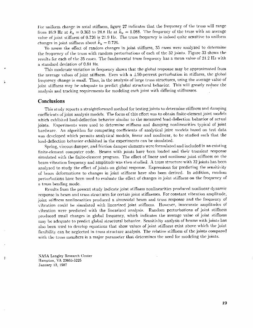
For uniform change in axial stiffness, figure 27 indicates that the frequency of tile truss will range
from 16.9 Hz at ku = 0.363 to 24.8 Hz at ku = 1.088. The frequency of the truss with an average
value of joint stiffness of 0.726 is 21.9 Hz. The truss frequency is indeed quite sensitive to uniform
changes in joint stiffness about ku = 0.726.
To assess the effect of random changes in joint stiffness, 35 cases were analyzed to determine
tile frequency of the truss with random perturbations of each of the 32 joints. Figure 33 shows the
results for each of the 35 cases. The flmdamental truss frequency has a mean value of 21.2 Hz with
a standard deviation of 0.81 Hz.
This moderate variation in frequency shows that the global response may be approximated from
the average values of joint stiffness. Even with a ±50-percent perturbation in stiffness, the global
frequency change is small. Thus, in the analysis of large truss structures, using the average value of
joint stiffness may be adequate to predict global structural behavior. This ,,'ill greatly reduce the
analysis and tracking requirements for modeling each joint with differing stiffnesses.
Conclusions
This study reports a straightforward method for testing joints to determine stiffness and damping
coefficients of joint analysis models. The focus of this effort was to obtain finite-element joint lnodelswhich exhibited load-deflection behavior similar to the measured load-deflection behavior of actual
joints. Experiments were used to determine stiffness and damping nonlinearities typical of joint
hardware. An algorithm for computing coefficients of analytical joint, models based on test data
was developed which permits analytical models, linear and nonlinear, to be studied such that the
load-deflection behavior exhibited in the experiments can be simulated.
Spring, viscous damper, and friction damper elements were formulated and included in an existing
finite-element computer code. Beams with joints have been loaded and their transient response
simulated with the finite-element program. The effect of linear and nonlinear joint stiffness on the
beam vibration frequency and amplitude was then studied. A truss structure with 32 joints has been
analyzed to study the effect of joints on globat response. Expressions for predicting the sensitivity
of beam deformations to changes in joint stiffness have also been derived. In addition, random
perturbations have been used to evaluate the effect of changes in joint, stiffness on the frequency of
a truss bending mode.
Results from the present, study indicate joint, stiffness nonlinearities produced nonlinear dynamic
response in beam and truss structures for certain joint stiffnesses. For constant vibration amplitude,
joint stiffness nonlinearities produced a sinusoidal beam and truss response and the frequency of
vibration could be simulated with linearized joint stiffness. However, inaccurate amplitudes of
vibration were predicted with the linearized analysis. Random perturbations of joint, stiffness
produced small changes in global frequency, which indicates the average value of joint stiffness
may be adequate to predict global structural behavior. Sensitivity analysis of beams with joints has
also been used to develop equations that show values of joint stiffness exist above which the joint
flexibility can be neglected in truss structure analysis. The relative stiffness of the joints compared
with the truss members is a major parameter that. determines the need for modeling the joints.
NASA Langley Research CenterHampton, VA 23665-5225January 13, 1987
19

References
1. Campbell, Thomas G.: Hoop/Column Antenna Tech-
nology Development Summary. Large Space Systems
Technology- 1980, Volume [--Systems Technology,
Frank Kopriver III, compiler, NASA CP-2168, 1981,
pp. 357 364.
2. Mikulas, Martin M., Jr.; Croomes, Scott D.;
Schneider, William; Bush, Harold G.; Nagy, Kornell;
Pelischek, Timothy; Lake, Mark S.; and Wesselski,
Clarence: Space Station Truss Structures and Construc-
tion Considerations. NASA TM-86338, 1985.
3. Ungar, Eric E.: Energy Dissipation at Structural Joints;
Mechanisms and Magnitudes. FDL-TDR-64-98, U.S. Air
Force, Aug. 1964.
4. Crema, Luigi Ralis; Castellani, Antonio; and Nappi,
Alfonso: Damping Effects in Joints and Experimen-
tal Tests of Riveted Specimens. Damping Effects
in Aerospace Structures, AGARD-CP-277, Oct. 1979,
pp. 12-1-12-17.
5. Ungar, E. E.: The Status of Engineering Knowl-
edge Concerning the Damping of Built-Up Structures.
J. Sound _ Vib., vol. 26, no. 1, Jan. 8, 1973,
pp. 141 154.
6. Beards, C. F.: Damping in Structural Joints. Shock
Vib. Dig., vol. 11, no. 9, Sept. 1979, pp. 35-41.
7. Aubert, Allen C.; Crawley, Edward F.; and O'Donnell,
Kevin J.: Measurement of the Dynamic Properties of
Joints in Flexible Space Structures. SSL 35-83 (Grant
NAGW-21), Space Systems Laboratory, Massachusetts
Institute of Technology, Sept. 1983.
8. Soni, M. L.; and Agrawal, B. N.: Damping Synthesis for
Flexible Space Structures Using Combined Experimen-
tal and Analytical Models. AIAA/ASME/ASCE/AHS
26th Structures, Structural Dynamics and Materials
Conference A Collection of Technical Papers, Part 2,
Apr. 1985, pp. 552 558. (Available as AIAA-85-0779.)
9. O'Donnell, Kevin J.; and Crawley, Edward F.: Identifi-
cation of Nonlinear System Parameters in Space Struc-
ture Joints Using the Force-State Mapping Technique.
SSL 16-85 (Grant NAGW-21), Space Systems Labora-
tory, Massachusetts Institute of Technology, July 1985.
10. Craig, R. R., Jr.: A Review of Time-Domain and
Frequency-Domain Component Mode Synthesis
Method. Proceedings of the Joint Mechanics Conference
on Combined Experimental/Analytical Modeling of Dy-
namic Structural Systems, American Society Mechanical
Engineers, 1985, pp. 1-30.
l l. Hurty, Walter C.: Dynamic Analysis of Structural Sys-
tems Using Component Modes. AIAA J., vol. 3, no. 4,
Apr. 1965, pp. 678 685.
12. Hurty, Walter C.; Collins, Jon D.; and Hart, Gary C.:
Dynamic Analysis of Large Structures by Modal Syn-
thesis Techniques. Comput. FJ Struct., vol. 1, no. 4,
Dec. 1971, pp. 535 563.
13. Craig, Roy R., Jr.; and Bampton, Mervyn C. C.: Cou-
pling of Substructures for Dynamic Analysis. AIAA J.,
vol. 6, no. 7, July 1968, pp. 1313-1319.
14. Goldman, Robert L.: Vibration Analysis by Dynamic
Partitioning. AIAA J., vol. 7, no. 6, June 1969,
pp. 1152 1154.
15. Benfield, W. A.; and Hruda, R. F.: Vibration Analysis of
Structures by Component Mode Substitution. AIAA J.,
vol. 9, no. 7, July 1971, pp. 1255-1261.
16. Kuhar, Edward J.; and Stahle, Clyde V.: Dynamic
Transformation Method for Modal Synthesis. AIAA J.,
vol. 12, no. 5, May 1974, pp. 672 678.
17. Dowell, E. H.: Free Vibrations of an Arbitrary Structure
in Terms of Component Modes. Trans. ASME, Ser. E:
J. Appl. Mech., vol. 39, no. 3, Sept. 1972, pp. 727-732.
18. Dowell, E. H.: Free Vibrations of a Linear Structure
With Arbitrary Support Conditions. Trans. ASME,
Set. E: J. Appl. Mech., vol. 38, no. 3, Sept. 1971,
pp. 595 600.
19. Klein, L. R.; and Dowell, E. H.: Analysis of Modal
Damping by Component Modes Method Using Lagrange
Multipliers. Trans. ASME, Set. E: J. Appl. Mech.,
vol. 41, no. 2, June 1974, pp. 527 528.
20. Dowell, E. H.: Component Mode Analysis of Nonlinear
and Nonconservative Systems. J. AppI. Mech., vol. 47,
no. l, Mar. 1980, pp. 172-176.
21. Lazan, Benjamin J.: Damping of Materials and Members
in Structural Mechanics. Pergamon Press, c.1968.
22. Vanderplaats, G. N.: ADS--A FORTRAN Program
for Automated Design Synthesis-- Version 1.00. NASA
CR-172460, 1984.
23. Dompka, Robert V.: Improved Analytic Simulation of
Impact Dynamics. M.S. Thesis, George Washington
Univ., Feb. 3, 1984.
24. Noor, Ahmed K.; and Peters, Jeanne M.: Penalty Fi-
nite Element Models for Nonlinear Dynamic Analy-
sis. AIAA/ASME/ASCE/AHS 26th Structures, Struc-
tural Dynamics and Materials Conference--A Collection
of Technical Papers, Part 2, Apr. 1985, pp. 36_378.
(Available as AIAA-85-0728.)
25. Reissner, Eric: On One-Dimensional Finite-Strain Beam
Theory: The Plane Problem. Z. Angew. Math. _ Phys.,
vol. 23, Fasc. 5, Sept. 25, 1972, pp. 795 804.
q[
20
l[| Ii

ORIQ)NAL PAGE ISDF POOh QUAUTY
Figure 1. Hoop-column antenna.
21

22
II| !ll

0 Force
0 Displacement
0
Velocity
Figure 3. Example of a force-state map.
Assume type of analysis model
that represents joint load-deflection behavior
Main 1path
Conduct experiments to determinejoint load-deflection behavior
Alternate
path
Curve-fit experimental data I_
using analysis model and optimization algorithm C
Figure 4. Flowchart for empirical joint model development.
23

j_Maxwell
model __
tStandard
anelastic model
Modified standardanelastic model
Figure 5. Empirical joint models for material stiffness and damping analysis.
Figure 6. Sign convention for MSA model.
24
Ill Ii

Ft
kaI I-
////
_c
Ff
///
X Constant coefficients
Ff
//
!I
F t"I
IT j II
II
/// X
//
Shape functions
"l"-f ,, X
t "F ¢j,
s/ Xs
Variable coefficients
FI,/;#
C/] X
.;.[..';_,q x
:]'/J, _
," X
Figure 7. Load-deflection shape functions for constant and variable coefficients.
-F
I /I lope= kI
I mX!I---II
CI
tFigure 8. Load-deflection behavior with joint dead band.
25

!-
TF
Ff
f_k"]c
"F
Figure 9. Two-node empirical joint model.
ct_k a
Ff _ kb
_k c
MSA model
F
kk
c
F
Two-nodenonlinear model
Ff
F
Two-nodelinear model
Figure 10. General models for joint simulations.
2{}

(a) Clusterjoint. (b) Clevisjoint.
Figurel l. Typicaltrussjoints for spaceapplications.
2700
1620
540
L_bd'
-540
-1620
-2700 I I
-.I0 -.06 -.02 .02 .06
Deflection,in.
I
.I0
Figure 12. Joint load-deflection test data measured at frequency of 1 Hz.
27

CI
"l
Set damping = 0Solve for stiffness )
I Set stiffness = pass 1 i_Solve for damping
Set stiffness = pass I )_Damping = pass 2
I Print final I_stiffness damping
Pass I
Pass 2
Pass 3
_-----[ Minimize 0 lSolve for stiffnessI
.,..._I
-'--I Minimize 0Solve for dampingI
"_--[ Minimize 0 Istiffness damping
Figure 13. Three-pass solution strategy used in present study.
Load,Ib
I00 -
20-
-20 -
-60 -
-I00
-1.0
Simulated
Curve fit
I I I
-.6 -.2 .2 .6 1.0
Deflection,in.
Figure 14. Load-deflection curve fit with simulated data and constant-coefficient MSA model.
28

Load,lb
100
6O
2O
-2O
-6O
-I00
-.5
m
-- "W
I 1 f-.3 -.I .I .3 .5
Deflection, in.
Simulated
Curve fit
Figure 15. Load-deflection curve fit with nonlinear simulated data and constant-coefficient MSA model.
100
5O
20
L_bd'-20
-60
-100 I_5 -.3 -.1 .1 .3 .5
Deflection, in.
Simulated
Curve fit
Figure 16. Load-deflection curve fit with nonlinear simulated data and variable-coefficient MSA model.
29

Load,lb
2700
1620
54O
-540 -
-1620 -
-2700-.10
m
m
I I
Test
Curve fit
I-. 06 -. 02 .02 .06 . I0
Deflection, in.
Figure 17. Load-deflection curve fit with test data and variable-coefficient MSA model.
F
Node a Node b
_- \\\\\\\ -- -"-Fr
Figure 18. Spring element sign convention.
30
I!| i!]

k o Beam
Z/2
1
F Step load
'////////2t
\\ \\-
Figure 19. Built-in beam with end joints.
Frequencyratio,
_OSS
3
2
1
0 I i i i i |11] [ J i | i [11] j. j
0.I 1.0 I0.0
Rotational stiffness parameter, k0
I I till
100.0
Figure 20. Effect of joint rotational stiffness on beam frequency.
31

Lateral
displacement,ino
.O5
.O4
O3
.01
0 .025
Figure 21.
ii r| I tl
,, , ' i'i i : ,,
t I
Il I tI
• 075 .100 •125
sec
Effect of nonliqear joint stiffness on beam response.
Linear
..... Nonlinear
Lateral
displacement,in.
• • t _ F #1 II __05 , ,, ....11 Ii II i t I I I I I!
i tl ii t I I i I tl
II t I tl I tl
t i t i _ ! I tI I I I I
O4 I I I ! I I I w I• l I I ! I I I I I I
I t _ I t i f i
J I I I
I I i I t I
f I i ! Ii I t I ! I
I I ii
it I J I t
Ii I I !
I i.02 : :I !
I ! I _ I
I I tI ! tI I
! t t t
t t I
01 ' it I I
• II I I
t s ti t
• I I
0 . 025 . 050 . 075 . 100 . 125
Time, sec
Figure 22. Effect of joint dead band on beam response.
Linear
Nonlinear
32
II| ill

Lateral
displacement,in.
• O5
.O4
.03
• 02
.01
0 .025
r jt r
• 050 .075 .100 .125
Time, sec
Linearized
Nonlinear
(a) For hardening nonlinearity.
Figure 23. Beam response with linearized joint stiffness.
Lateral
displacement,in.
• 05II II
II 'I
I I i I
I I I I
¢ I I !
I I I
.03 1
.02
.01
! i
I I 11 Ii _ It n
i i I I| ft Ii ii¢1 ! it
I t ¢1 ii i_ i
o i t Ii i I iim I i i i .....
! ! | i ! i !
i t f i ! i !i i ! |
I I I I II I
I
I ! ! I 1 1 I I
i ! i 1
° II
! I I I I I
i ' 'I !
i |
I i
I i !
i !
I !
! I
i I
j I
j I
!
! I
L Q i !
• 025 .050 .075 .100 .125
Time, sec
(b) For dead band nonlinearity.
Figure 23. Concluded.
-- linearized
Nonlinear
33

Lateral
displacement,in.
11
I
I I
!
Linearized
Nonlinear
I 1 I
0 .025 .050 .075 .100 .125
Time, sec
Figure 24. Viscous damped beam response with nonlinear and linearized joint stiffness.
Lateral
displacement,in.
• O5
.O4
.O3
. O2
.0I
q
I
I
¢ I
I
!
11
I
I
I
I
I
I I
0 .025 .100 .125
Linearized
..... Nonlinear
Figure 25. Friction damped beam response with nonlinear and linearized joint stiffness.
34
I1| 1i

//////I///
S,-------__I
F [Step load
V///.,'.t
A
F
Ti
Figure 26. Cantilevered, four-bay truss with joints.
Fundamental
frequency,Hz
4O
30
20
10
0 I , , i i_,tl I n I In Ijll
0.1 1.0 10.0
Axial stiffness parameter, kU
I I I I Illll
100.0
Figure 27. Effect of joint axial stiffness on truss frequency.
35

Lateral
displacement,in.
• O8
• O6
.O4
• O2
0
I
I
!
I
t
1
I
I
I
I
I
I
I
t
t
t
I
I
1
I
t
I
I
I
I
t
I t
II t I "t Ir
I I 1 I I
I _" I I I
f I ! I I I
• 04 .08 .12 .16 .20
Time, sec
Figure 28. Effect of joint dead band on truss frequency.
Linear
Nonlinear
. O8
• O6
Lateral
displacement,in.
.O4
.O2
Figure 29.
0
tr I
tI I
II I
t! I
tI I
I !I
! I
! - i I t
l I I I ! t
I L ! t I I
! t I t I I
I I I I r I
I ' • 1 I I
I , ' , ; t ,
I I t I I
I f I I
I I I t ! t t I
I I I I I
ii ti , j _,111 • I
• 04 .08 .12 .16 .20
Time, sec
Linearized
Nonlinear
Truss response with linearized joint stiffness for dead band nonlinearity.
36
IrF,1i

Lateral
displacement,in.
.08
.06
.04
• 02
0
,s t ,t • f
, t l I ; t
l I I t I i
' l I r
! , I , I
I I I
I , l
I I I
I I
p ! 1 I |
, I r !
! j I I I
, | f I , I J
I ' J l #! t j I
I I _ I t ,r
] I I ] I
.04 . 08 . 12 . 16 .20
Nonlinear,friction damped
..... Non linear,
undamped
Time, sec
Figure 30. Friction damped truss response with nonlinear joint stiffness.
d
(a) Two-node beam.
Node cA
_TNode"d
Node b __" SJ
Node
(b) Four-node beam.
Figure 31. Beams used in deformation sensitivity study.
37

Displacementratio,
uj
u R
4
3
2
tI I
0 10 2O
Axialstiffnessparameter,ku
J
3O
Figure 32.
(a) Variation of axial stiffness.
Sensitivity of beam deformations to joint stiffness.
Displacementratio,
wj
wR
I
Lateral
I II0 20
stiffness parameter, k'w
(b) Variation of lateral stiffness.
Figure 32. Continued.
!3O
38
II_:I!

m
Displacementratio,
¢)J
e R
2
1
0I I
I0 20
Rotational stiffness parameter,
(c) Variation of rotational stiffness.
Figure 32. Concluded.
N
k¢
I30
39

30-
Frequency,Hz
25
2O
15-
10
I I I I10 20 30 40
Number of case
k u = 1.088
k" = O.726U
N
k = 0.323U
Figure 33. Sensitivity of truss frequency to random perturbations of joint axial stiffness.
4O
IEI_]i

Report Documentation Page
1. Report No. I 2. Government Accession No.
NASA TP-2661 14. Title and Subtitle
Modeling of Joints for the Dynamic Analysis of Truss Structures
3. Recipient's Catalog No.
5. Report Date
May 1987
6. Performing Organization Code
8. Performing Organization Report No.
L-16163
10. Work Unit No.
506-43-51-02
ll. Contract or Grant No.
13. Type of Report and Period Covered
Technical Paper
14. Sponsoring Agency Code
7. Author(s)W. Keith Belvin
9. Performing Organization Name and Address
NASA Langley Research CenterHampton, VA 23665-5225
12. Sponsoring Agency Name and Address
National Aeronautics and Space AdministrationWashington, DC 20546-0001
15. Supplementary Notes
16. Abstract
An experimentally-based method for determining the stiffness and damping of truss joints is
described. The analytical models use springs and both viscous and friction dampers to simulate
joint load-deflection behavior. A least-squares algorithm is developed to identify the stiffness and
damping coefficients of the analytical joint models from test data. The effects of nonlinear jointstiffness such as joint dead band are also studied. Equations for predicting the sensitivity of beam
deformations to changes in joint stiffness are derived and used to show the level of joint stiffness
required for nearly rigid joint behavior. Finally, the global frequency sensitivity of a truss structureto random perturbations in joint stiffness is discussed.
17. Key Words (Suggested by Authors(s))Joints
Truss structures
Joint-dominated structures
Modeling
Large space structures
19. Security Classif.(of this report) I
Unclassified INASA FORM 1626 OCT 86
18. Distribution Statement
Unclassified - Unlimited
Subject Category 39
20, Security Classif.(of this page) I 21. No. of Pages 22. Price
Unclassified ] 41 A03
NASA-Langley, 1987
For sale by the National Technical Information Service, Springfield, Virginia 22161-2171

11F