Santosh K. SahuSukanya Das

MADRAS SCHOOL OF ECONOMICSGandhi Mandapam Road

Chennai 600 025 India

October 2015

IMPACT OF AGRICULTURAL RELATED TECHNOLOGY ADOPTION ON POVERTY:

A STUDY OF SELECT HOUSEHOLDS IN RURAL INDIA

MSE Working Papers

Recent Issues

* Working Paper 120/2015Health Shocks and Coping Strategies: State Health Insurance Scheme of Andhra Pradesh, IndiaSowmya Dhanaraj

* Working Paper 121/2015Efficiency in Education Sector: A Case of Rajasthan State (India)Brijesh C Purohit

* Working Paper 122/2015Mergers and Acquisitions in the Indian Pharmaceutical SectorSantosh Kumar Sahu and Nitika Agarwal

* Working Paper 123/2015Analyzing the Water Footprint of Indian Dairy IndustryZareena B. Irfan and Mohana Mondal

* Working Paper 124/2015Recreational Value of Coastal and Marine Ecosystems in India: A Partial EstimatePranab Mukhopadhyay and Vanessa Da Costa

* Working Paper 125/2015Effect of Macroeconomic News Releases on Bond Yields in India China and JapanSreejata Banerjee and Divya Sinha

* Working Paper 126/2015Investigating Household Preferences for Restoring Pallikaranai MarshSuganya Balakumar and Sukanya Das

* Working Paper 127/2015The Culmination of the MDG's: A New Arena of the Sustainable Development GoalsZareena B. Irfan, Arpita Nehra and Mohana Mondal

* Working Paper 128/2015Analyzing the Aid Effectiveness on the Living Standard: A Check-Up on South East Asian CountriesZareena B. Irfan, Arpita Nehra and Mohana Mondal

* Working Paper 129/2015Related Party Transactions And Stock Price Crash Risk: Evidence From IndiaEkta Selarka and Subhra Choudhuryana Mondal

* Working Paper 130/2015Women on Board and Performance of Family Firms: Evidence from India Jayati Sarkar and Ekta Selarka

* Working papers are downloadable from MSE website http://www.mse.ac.in

$ Restricted circulation

WORKING PAPER 131/2015

i

Impact of Agricultural Related Technology Adoption on Poverty: A Study of Select

Households in Rural India

Santosh K. Sahu Assistant Professor, Madras School of Economics

santosh@mse.ac.in

and

Sukanya Das Assistant Professor, Madras School of Economics

sukanya@mse.ac.in

ii

WORKING PAPER 131/2015

November 2015

Price : Rs. 35

MADRAS SCHOOL OF ECONOMICS

Gandhi Mandapam Road

Chennai 600 025

India

Phone: 2230 0304/2230 0307/2235 2157

Fax : 2235 4847/2235 2155

Email : info@mse.ac.in

Website: www.mse.ac.in

iii

Impact of Agricultural Related Technology Adoption on Poverty: A Study of Select

Households in Rural India

Santosh K. Sahu and Sukanya Das

Abstract

This paper applies a program evaluation technique to assess the causal effect of adoption of agricultural related technologies on consumption expenditure and poverty measured by different indices. The paper is based on a cross-sectional household level data collected during 2014 from a sample of 270 households in rural India. Sensitivity analysis is conducted to test the robustness of the propensity score based results using the “rbounds test” and the mean absolute standardized bias between adopters and non-adopters. The analysis reveals robust, positive and significant impacts of agricultural related technologies adoption on per capita consumption expenditure and on poverty reduction for the sample households in rural India.

Keywords: Agriculture related technology adoption, propensity score matching, poverty, Odisha, India

JEL Codes: C13, C15, O32, O38

iv

ACKNOWLEDGEMENT

We would like to thank the participants of the workshop on “Harnessing Technology for Challenging Inequality” at Tata Institute of Social Sciences, Mumbai jointly organized with Forum for Global Knowledge Sharing. We gratefully acknowledge Prof. K. Narayanan and Prof. N. S. Siddharthan for comments and suggestions in the earlier draft of this paper. We are grateful to MSSRF-APM Project for the funding support of the sub-project on PDHED at MSE Chennai. We gratefully acknowledge the inputs from Prof. U. Sankar, Prof. R. N. Bhattacharyya, Prof. K. R. Shanmugam, and Dr. A. Nambi for the insightful comments and suggestions on the project output. We also grateful acknowledge the respondents for their active participation during the primary data collection.

Santosh K. Sahu

Sukanya Das

1

INTRODUCTION

Growth in agricultural output is one of the most effective means to

address poverty in the developing world. In this line of argument, the

Department for International Development (2003) estimates that a one

percent increases in agricultural productivity could reduce poverty

between 0.6 and 2 percent. However, growing population is one of the

major challenges in developing countries to increase agricultural

productivity in a sustainable way, to meet the demand of the food

security issues. The growth in production cannot come from area

expansion but have to come from growth in yields emanating from

scientific advances offered by biotechnology and other plant breeding

initiatives (de-Janvry et al., 2001). In the increasing research of improved

varieties of major crops that enhanced the productivity of agriculture,

impact assessment studies were conducted to arrive at the direct and the

indirect welfare impacts. Kijima et al., (2008) in Uganda conducted a

study on the impact of rice, and found that rice adoption reduces poverty

without deteriorating the income distribution. Similarly, Winters et al.,

(1998); Mwabu et al., (2006); and Wu et al., (2010) show positive impact

of agricultural technologies adoptions. However, there are serious

complexities associated with understanding the impact pathways through

which agricultural technology adoption might affect household welfare.

This is because crop production can affect household welfare both

directly and indirectly. Consistent with this notion, de Janvry et al.,

(2001) reports that crop production affects poverty directly by raising

welfare of poor farmers who adopt the technological innovation, through

increased production for home consumption, higher gross revenues from

sales, lower production costs, and lower yield risks. The indirect ways

through which crop production affects welfare include the prices of food

for net buyers and employment and wage effects in agriculture and

related activities.

2

In a poor and backward state like Odisha in India, it is least

expected that the development scenario of the village and the pace of

socio-economic transformations could be better. The state has to make a

longitudinal perspective plan for the transformation of the subsistence

oriented backward agricultural economy in order to solve the problem of

poverty and to improve the „quality of life‟ of rural people. Dependence of

population on primary sector occupations is quite high, whereas

agriculture with its present state of infrastructure and technology and,

above all, operational holdings is itself not in a position to provide a

substantial form of gainful livelihood to the majority of rural population in

Odisha. There have been little occupational diversifications of population

at the village level. Irrigation infrastructure created through many

development projects has failed to achieve desired goal across space and

people. Often this serves the interest of only large, medium and semi-

medium farmers. Like this, the welfare programmes and Minimum Needs

Programme implemented by the state under social sector development to

lessen poverty and improve the „quality of life‟ of poor in rural areas

hardly reach the targeted sections of population.

In a poor and backward state showing highest incidence of rural

poverty, the development of hardcore backward districts requires special

attention. It is found that the socio-economic conditions of people in the

undivided Kalahandi, Bolangir and Koraput districts, popularly known as

the KBK districts, have worsened over the years. These three districts

have been affected by the „backwash effects‟ of development, which may

probably be due to their inherent disadvantageous factors like poor

quality of human capital, backward and unsustainable agriculture coupled

with reckless exploitation of forest resources. This study is an attempt to

see the impact of agricultural technology adoption on poverty of the

select households of the Jeypore sub-division of the Koraput district of

Odisha state.

3

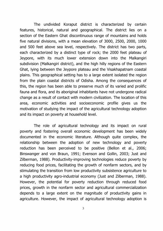
The undivided Koraput district is characterized by certain

features, historical, natural and geographical. The district lies on a

section of the Eastern Ghat discontinuous range of mountains and holds

five natural divisions, with a mean elevation of 3000, 2500, 2000, 1000

and 500 feet above sea level, respectively. The district has two parts,

each characterized by a distinct type of rock; the 2000 feet plateau of

Jeypore, with its much lower extension down into the Malkangiri

subdivision (Malkangiri district), and the high hilly regions of the Eastern

Ghat, lying between the Jeypore plateau and the Visakhapatnam coastal

plains. This geographical setting has to a large extent isolated the region

from the plain coastal districts of Odisha. Among the consequences of

this, the region has been able to preserve much of its varied and prolific

fauna and flora, and its aboriginal inhabitants have not undergone radical

change as a result of contact with modern civilization. The location of this

area, economic activities and socioeconomic profile gives us the

motivation of studying the impact of the agricultural technology adoption

and its impact on poverty at household level.

The role of agricultural technology and its impact on rural

poverty and fostering overall economic development has been widely

documented in the economic literature. Although quite complex, the

relationship between the adoption of new technology and poverty

reduction has been perceived to be positive (Bellon et al., 2006;

Binswanger and von Braun, 1991; Evenson and Gollin, 2003; Just and

Zilberman, 1988). Productivity-improving technologies reduce poverty by

reducing food prices, facilitating the growth of nonfarm sectors, and by

stimulating the transition from low productivity subsistence agriculture to

a high productivity agro-industrial economy (Just and Zilberman, 1988).

However, the potential for poverty reduction through reduced food

prices, growth in the nonfarm sector and agricultural commercialization

depends to a large extent on the magnitude of productivity gains in

agriculture. However, the impact of agricultural technology adoption is

4

necessary to understand at farm-household level. It is also important to

distinguish between the direct and the indirect impact of the impact of

such technology adoption (Becerril and Abdulai, 2010; David and Otsuka,

1994; de Janvry and Sadoulet, 2002; Minten and Barrett, 2008; Moyo et

al., 2007).

The direct effects of new agricultural technology on poverty

reduction are the productivity benefits enjoyed by the farmers adopting

new technology. These benefits usually manifest themselves in the form

of higher farm incomes. The indirect effects are productivity- induced

benefits passed on to others by the adopters of the technology. These

may comprise lower food prices, higher nonfarm employment levels or

increases in consumption for all farmers (de Janvry and Sadoulet, 2002).

However, productivity- enhancing agricultural technology involves a

bundle of innovations rather than just a single technology. The impacts

of higher-order (indirect) benefits from technology adoption depend:

depend on the elasticity of demand, outward shifts in supply lowering

food prices; and an increased productivity which may stimulate the

demand for labor. The poor and marginal farmers tend to supply off-farm

labor, which may translate to increased employment, wages, and

earnings for them. They have little or no land and they gain

disproportionately from employment generated by agricultural growth

and from lower food prices. Higher productivity can, therefore, stimulate

broader development of the rural economy through general equilibrium

and multiplier effects, which also contribute to poverty reduction.

Agricultural technology may induce changes in cropping patterns and

allocation of farmers‟ own resources to different uses. It is important to

notice that the technology adoptions may vary from farmer to farmer and

the nature of the technology in use. For instance, technology adoption in

agriculture can be either through high yield variety (HYV) seeds,

advances in irrigation facilities, fertilizers, pesticides use or through the

machinery employed during agricultural activities.

5

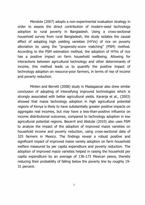
Mendola (2007) adopts a non-experimental evaluation strategy in

order to assess the direct contribution of modern-seed technology

adoption to rural poverty in Bangladesh. Using a cross-sectional

household survey from rural Bangladesh, the study isolates the causal

effect of adopting high yielding varieties (HYVs) of rice on poverty

alleviation by using the “propensity-score matching” (PSM) method.

According to the PSM estimation method, the adoption of HYVs of rice

has a positive impact on farm household wellbeing. Allowing for

interactions between agricultural technology and other determinants of

income, this method leads us to quantify the positive impact of

technology adoption on resource-poor farmers, in terms of rise of income

and poverty reduction.

Minten and Berrett (2008) study in Madagascar also drew similar

conclusion of adopting of intensifying improved technologies which is

strongly associated with better agricultural yields. Karanja et al., (2003)

showed that maize technology adoption in high agricultural potential

regions of Kenya is likely to have substantially greater positive impacts on

aggregate real incomes, but may have a less-than-positive influence on

income distributional outcomes, compared to technology adoption in low

agricultural potential regions. Becerril and Abdulai (2010) also uses PSM

to analyze the impact of the adoption of improved maize varieties on

household income and poverty reduction, using cross-sectional data of

325 farmers in Mexico. The findings reveal a robust positive and

significant impact of improved maize variety adoption on farm household

welfare measured by per capita expenditure and poverty reduction. The

adoption of improved maize varieties helped in raising the household per

capita expenditure by an average of 136-173 Mexican pesos, thereby

reducing their probability of falling below the poverty line by roughly 19-

31 percent.

6

Most of the studies on the impact of agricultural technology on

farm incomes and poverty reduction focus macro approaches, with very

few analyses at the micro-level. Some of the few household level studies

include Evenson and Gollin (2003); Mendola (2007); and Moyo et al.,

(2007). Kassie et al., (2011) evaluates the ex-post impact of adopting

improved groundnut varieties on crop income and poverty in rural

Uganda. The study utilizes cross-sectional data of 927 households,

collected in 2006, from seven districts in Uganda. Using PSM technique

the study reports that adopting improved groundnut varieties

(technology) significantly increases crop income and reduces poverty.

Thus, the literature appears to document overall positive

impacts, with far less evidence at the individual household level that

specifically show the effects of the adoption of agricultural technologies

on farm productivity and household welfare. This study is a value

addition in this regard in the context of Odisha. The objective of this

paper is to assess the role of agriculture related technology adoption, on

consumption expenditure and poverty status measured by headcount

index, poverty gap index and poverty severity index. The empirical

question that we would like to address is “do agriculture related

technology adoptions have the potential to reduce poverty?” In

understanding this question, we apply PSM method to deal with the

selection bias problem. In addition to PSM, we also conduct the “rbounds

test” and a “balancing test” using the “mean absolute standardized bias”

between the agricultural technology adopters and non-adopters as

suggested in Rosenbaum and Rubin (1985). The rest of the paper is

organized as follows. Section-2 presents the analytical framework and the

model, section-3 presents the data and descriptive statistics, section-4

presents the econometric results and section-5 concludes.

7

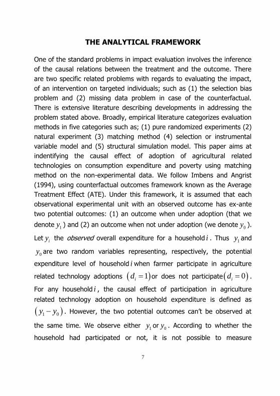
THE ANALYTICAL FRAMEWORK

One of the standard problems in impact evaluation involves the inference

of the causal relations between the treatment and the outcome. There

are two specific related problems with regards to evaluating the impact,

of an intervention on targeted individuals; such as (1) the selection bias

problem and (2) missing data problem in case of the counterfactual.

There is extensive literature describing developments in addressing the

problem stated above. Broadly, empirical literature categorizes evaluation

methods in five categories such as; (1) pure randomized experiments (2)

natural experiment (3) matching method (4) selection or instrumental

variable model and (5) structural simulation model. This paper aims at

indentifying the causal effect of adoption of agricultural related

technologies on consumption expenditure and poverty using matching

method on the non-experimental data. We follow Imbens and Angrist

(1994), using counterfactual outcomes framework known as the Average

Treatment Effect (ATE). Under this framework, it is assumed that each

observational experimental unit with an observed outcome has ex-ante

two potential outcomes: (1) an outcome when under adoption (that we

denote1y ) and (2) an outcome when not under adoption (we denote

0y ).

Letiy the observed overall expenditure for a household i . Thus

1y and

0y are two random variables representing, respectively, the potential

expenditure level of household i when farmer participate in agriculture

related technology adoptions 1id or does not participate 0id .

For any household i , the causal effect of participation in agriculture

related technology adoption on household expenditure is defined as

1 0y y . However, the two potential outcomes can‟t be observed at

the same time. We observe either 1y or

0y . According to whether the

household had participated or not, it is not possible to measure

8

1 0y y directly. The average causal effect of adoption within a specific

population (ATE) can be determined as 1 0E y y , with E as the

mathematical expectation.

Several methods have been proposed to estimate ATE, and they

include the matching methods based on propensity scores, as well as

parametric methods based on Instrumental variable methods. The choice

of method is largely driven by the assumptions made and the availability

of data. For any observational data (that is non-experimental) an

important assumption is; the Conditional Independence Assumption

(CIA), that states conditional on X (observables), the outcomes are

independent of the treatment d and can be written as:

1, 0 |y y d X (1)

The behavioral implication of this assumption is that participation

in the treatment does not depend on the outcomes after controlling for

the variation in outcomes induced by differences in X . A much weaker

assumption also used for indentifiability of the causal effect of the

treatment is what Imbens and Angrist (1994) refers to as the

unconfoundedness assumption, and which Rubin (1978) refers to as the

ignorability assumption. The assumption is written as:

0 |y d X (2)

If valid, the assumption implies that there is no omitted variable

bias once X is included in the equation hence there will be no

confounding. The assumption of unconfoundedness (equation-2) is very

strong, and its plausibility heavily relies on the quality and the amount of

information contained in X . A slightly weaker assumption also associated

9

with the treatment effect evaluation is referred to as the “overlap or

matching (common-support condition)” assumption. The assumption

ensures that for each value of X , there are both treated and untreated

cases. The assumption is expressed as follows:

0 Pr 1| 1d X (3)

This implies that there is an overlap between the treated and

untreated samples. Stated the other way round this also means that the

control and treated populations have comparable observed

characteristics. Under the assumption discussed above (CIA and overlap)

the ATE on the Average Treatment Treated (ATT) can be identified as:

1 0 1 0

1 0

| 1 | 1,

| 1, | 0, | 1

E y y a E E y y d X

E E y d X E y d X d

(4)

Where, the outer expectation is over the distribution of X , in the

subpopulation of participating households in agricultural related

technologies. In observational data, it is not possible to calculate directly

the difference in the outcome of interest between the treated and the

control group or the ATE due to the absence of the counterfactual1. As a

consequence, data may be drawn from comparison units whose

characteristics match those of the treated group. The average outcome

of the untreated matched group is assumed to identify the mean

counterfactual outcome for the treated group in the absence of a

treatment. The propensity score matching method matches treated and

untreated cases on the propensity score rather than on the regressor.

1 The counterfactual is a condition in which the same household is observed under treatment and

without treatment. In reality a household can only be observed under either of the two conditions

at a time and not under both.

10

The propensity score which is the conditional probability of receiving

treatment given X , is denoted P x written as:

Pr 1|p x d X x (5)

An assumption that plays an important role in treatment

evaluation is the balancing condition which states that;

|d X p x (6)

This can be expressed alternatively by stating that, for individuals

with the same propensity score the assignment to treatment is random

and should look identical in terms of their x vector. The main purpose of

the propensity score estimation is to balance the observed distribution of

covariates across the groups of adopters and non-adopters (Lee, 2005).

The balancing test is normally required after matching to ascertain

whether the differences in the covariates in the two groups in the

matched sample have been eliminated, in which case, the matched

comparison group can be considered a plausible counterfactual (Ali and

Abdulai, 2010). Although several versions of balancing tests exist in the

literature, the most widely used is the mean absolute standardized bias

(MASB) between adopters and non-adopters (Rosenbaum and Rubin,

1985). Additionally, Sianesi (2004) proposed a comparison of the pseudo

2R and p-values of the likelihood ratio test of the joint significance of all

the regressors obtained from the logit analysis before and after matching

the samples.

After matching, there should be no systematic differences in the

distribution of covariates between the two groups. As a result, the

pseudo 2R should be lower and the joint significance of covariates

11

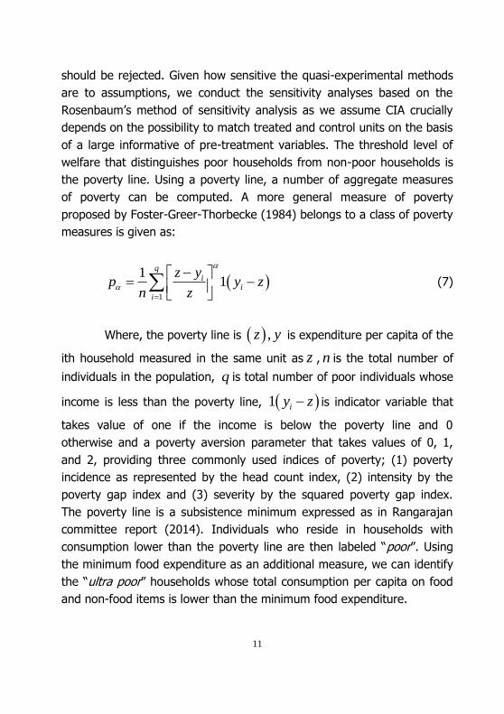
should be rejected. Given how sensitive the quasi-experimental methods

are to assumptions, we conduct the sensitivity analyses based on the

Rosenbaum‟s method of sensitivity analysis as we assume CIA crucially

depends on the possibility to match treated and control units on the basis

of a large informative of pre-treatment variables. The threshold level of

welfare that distinguishes poor households from non-poor households is

the poverty line. Using a poverty line, a number of aggregate measures

of poverty can be computed. A more general measure of poverty

proposed by Foster-Greer-Thorbecke (1984) belongs to a class of poverty

measures is given as:

1

11

q

ii

i

z yp y z

n z

(7)

Where, the poverty line is ,z y is expenditure per capita of the

ith household measured in the same unit as z , n is the total number of

individuals in the population, q is total number of poor individuals whose

income is less than the poverty line, 1 iy z is indicator variable that

takes value of one if the income is below the poverty line and 0

otherwise and a poverty aversion parameter that takes values of 0, 1,

and 2, providing three commonly used indices of poverty; (1) poverty

incidence as represented by the head count index, (2) intensity by the

poverty gap index and (3) severity by the squared poverty gap index.

The poverty line is a subsistence minimum expressed as in Rangarajan

committee report (2014). Individuals who reside in households with

consumption lower than the poverty line are then labeled “poor”. Using

the minimum food expenditure as an additional measure, we can identify

the “ultra poor” households whose total consumption per capita on food

and non-food items is lower than the minimum food expenditure.

12

DATA AND DESCRIPTIVE STATISTICS

The data were collected through a household survey conducted in

Koraput district of Odisha state in India. The sample villages are the

beneficiaries of various programmes of M. S. Swaminathan Research

Foundation (MSSRF) initiatives on technologies related to agriculture. The

households were randomly selected from Jeypore sub-district. This led to

the selection of 296 households. Data were collected at village and farm-

household levels. At the village level, data collected included crops grown

and the village infrastructures. At the household level data collected

included the farmer knowledge of varieties cultivated, household

composition and characteristics, land and non-land farm assets, livestock

ownership, household membership to different rural institutions, varieties

and area planted, indicators of access to infrastructure, household

market participation, household income sources and consumption

expenses. In this study, adopters are classified as households who have

adopted at least one of the agricultural technologies, out of maximum of

17 technologies as reported by the sample households during the primary

survey. These technologies are in terms of “asset related” to “technology

related” suitable for agricultural activities such as use of tractors, motor

for irrigation etc. weighted against the land holding (net). Table-1 reports

descriptive statistics, disaggregated at the adoption status.

Table 1 presents a comparison of some of the important

indicators at household level distinguished between adaptors and non-

adopters. We can observe from the table that income, income less from

MGNREGA, expenses related to food and total expenses, share of income

from primary and secondary sources, are statistically significant between

two groups. However, expenses related to non-food, income from tertiary

source, age and education of head of households are not statistically

different between both the groups. Therefore, determinants of poverty

can be different or similar based on the variables that are statistically

different. Further, we also know that there are trade-offs in technology

13

that generates direct and indirect effects. When land is unequally

distributed, and if there are market failures and conditions of access to

public goods that vary with farm size, then the optimum farming systems

will differ across farms. Small holder may opt to adopt capital saving

technologies, while larger farmers may prefer capital intensive

technologies.

Table 1: Household Characteristics by Adoption Status

Variables Non-adopters (n=107)

Adopters (n=189)

Full Sample (n=296)

Difference (t-test)

Total income 37297.680 48143.480 44222.870 2.495***

Income less from MGNREGA 36422.920 47202.210 43305.640 2.468***

Food expenses 18397.760 21339.760 20276.270 2.059***

Non-food expenses 5043.028 6289.159 5838.699 1.547

Total expenses 28098.790 34244.330 32022.800 2.354***

Share of income from primary Source 62.115 67.527 65.571 2.263***

Share of income from secondary source 23.773 19.806 21.240 2.362***

Share of income from tertiary Source 6.311 5.621 5.870 0.683

Age of head of household 45.607 43.042 43.970 1.535

Education of head of household 0.645 0.630 0.635 0.261

Source: Primary data collected by authors during 2014 Note: *** indicate statistically significant at 1%, MGNREGA- Mahatma Gandhi National

Rural Employment Guarantee Act, income and expenses are presented in Indian rupees, 2014

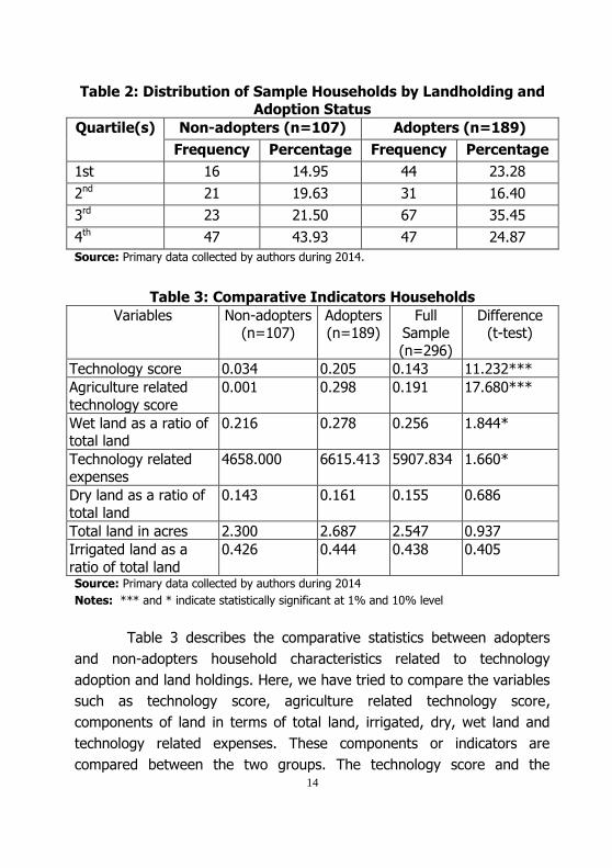
Table 2 presents the distribution of sample households according

to land holdings and adoption status. Consistent, with Bercerril and

Abdulai (2010), the differences in the distribution of land between

adopters and non-adopters suggest a positive correlation between the

incidence of adoption and the ownership of land. The incidence of

adoption is clearly higher among 1st and 3rd quartiles of land distribution

compared to the other two distributions. Such differences in land

ownership between adopter and non-adopters could also contribute to

the disparities in welfare indicators between the two groups.

14

Table 2: Distribution of Sample Households by Landholding and

Adoption Status

Quartile(s) Non-adopters (n=107) Adopters (n=189)

Frequency Percentage Frequency Percentage

1st 16 14.95 44 23.28

2nd 21 19.63 31 16.40

3rd 23 21.50 67 35.45

4th 47 43.93 47 24.87

Source: Primary data collected by authors during 2014.

Table 3: Comparative Indicators Households

Variables Non-adopters (n=107)

Adopters (n=189)

Full Sample

(n=296)

Difference (t-test)

Technology score 0.034 0.205 0.143 11.232***

Agriculture related

technology score

0.001 0.298 0.191 17.680***

Wet land as a ratio of total land

0.216 0.278 0.256 1.844*

Technology related expenses

4658.000 6615.413 5907.834 1.660*

Dry land as a ratio of

total land

0.143 0.161 0.155 0.686

Total land in acres 2.300 2.687 2.547 0.937

Irrigated land as a

ratio of total land

0.426 0.444 0.438 0.405

Source: Primary data collected by authors during 2014

Notes: *** and * indicate statistically significant at 1% and 10% level

Table 3 describes the comparative statistics between adopters

and non-adopters household characteristics related to technology

adoption and land holdings. Here, we have tried to compare the variables

such as technology score, agriculture related technology score,

components of land in terms of total land, irrigated, dry, wet land and

technology related expenses. These components or indicators are

compared between the two groups. The technology score and the

15

agriculture technology score are differentiated based on the technology

related to agriculture and non agriculture. The score for each of the

groups are defined as a weighted score that is similar to the Human

Development Index (HDI).

From table 3 we can observe that the sample, that is

differentiated based on the adopters and non-adopters are statistically

difference in terms of technology score, agriculture related technology

score, ratio of wet land to total land and expenses related to technology

at household level. Other than these variables, indicators such as ratio of

dry land to total land, total land and ratio between irrigated and total

land are not statistically different between two groups. Table-4 presents

mean and median per capita consumption expenditure and the Gini

coefficient by household grouped in different groups. There is a

significant difference between the adopter categories in terms of welfare

indictors.

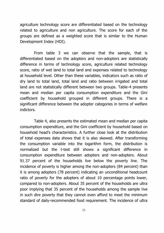
Table 4, also presents the estimated mean and median per capita

consumption expenditure, and the Gini coefficient by household based on

household head‟s characteristics. A further close look at the distribution

of total expenses data shows that it is also skewed. After transforming

the consumption variable into the logarithm form, the distribution is

normalized but the t-test still shows a significant difference in

consumption expenditure between adopters and non-adopters. About

91.37 percent of the households live below the poverty line. The

incidence of poverty is higher among the non-adopters (84 percent) than

it is among adopters (78 percent) indicating an unconditional headcount

ratio of poverty for the adopters of about 10 percentage points lower,

compared to non-adopters. About 35 percent of the households are ultra

poor implying that 35 percent of the households among the sample live

in such dire poverty that they cannot even afford to meet the minimum

standard of daily-recommended food requirement. The incidence of ultra

16

poverty is also higher among non-adopters (46 percent) than among

adopters (39 percent) suggesting that agriculture related technology

adoption is positively correlated with wellbeing.

Table 4: Mean and Median Per Capita Consumption Expenditure, and the Gini Coefficient

Mean Median Gini

coefficient

Male headed households 18718.2 14435.2 30.5

Female headed households 12799.2 14435.2 25.0

Household adopted to agricultural

related technology

19120.6 14435.2 32.1

Household not adopted to agricultural

related technology

17324.8 14435.2 28.1

Full sample 18416.7 14435.2 30.5 Source: Primary data collected by authors during 2014.

Table 5: Sensitivity of Poverty Measures to the Choice of Indicator

Poverty Headcount

Rate

Poverty Gap

Squared Poverty

Gap

Actual 91.4 53.2 34.3

Without technology adoption

(absolute)

92.0 56.7 37.9

Without agricultural technology adoption (absolute)

93.5 59.7 41.1

With education 91.1 51.2 32.3

With technology score (relative) 89.7 49.1 30.3

With agricultural technology

score (relative)

87.2 44.1 25.9

Source: Primary data collected by authors during 2014.

Table 5 presents the sensitivity of poverty measures to choice of

indicator. This table gives the estimates of poverty headcount, poverty

gap and squared poverty gap with and without some of the important

indicators. For example, we can see that education reduces poverty up to

-0.3 percent, higher technology score helps in reducing poverty up to 1.9

17

percent and agriculture technology score helps reducing poverty up to

4.5 percent. All the other indicators and results are given in Table 5.

ECONOMETRIC RESULTS AND DISCUSSION

Although, the unconditional summary statistics and tests in the tables

above in general suggest that agriculture related technology adoption

may have a positive role in improving household wellbeing, these results

are only based on observed mean differences in outcomes of interest and

may not be solely due to agriculture related technology adoption. They

may instead be due to other factors, such as differences in household

characteristics.

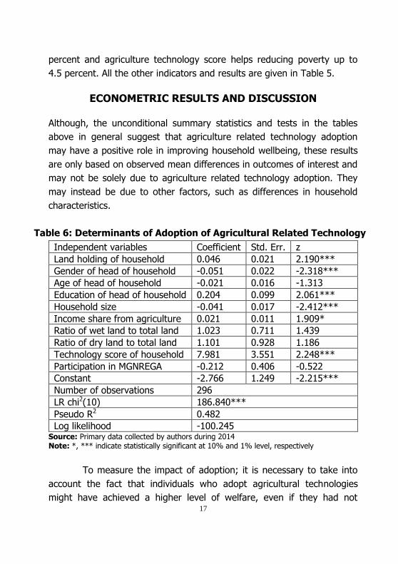
Table 6: Determinants of Adoption of Agricultural Related Technology

Independent variables Coefficient Std. Err. z

Land holding of household 0.046 0.021 2.190***

Gender of head of household -0.051 0.022 -2.318***

Age of head of household -0.021 0.016 -1.313

Education of head of household 0.204 0.099 2.061***

Household size -0.041 0.017 -2.412***

Income share from agriculture 0.021 0.011 1.909*

Ratio of wet land to total land 1.023 0.711 1.439

Ratio of dry land to total land 1.101 0.928 1.186

Technology score of household 7.981 3.551 2.248***

Participation in MGNREGA -0.212 0.406 -0.522

Constant -2.766 1.249 -2.215***

Number of observations 296

LR chi2(10) 186.840***

Pseudo R2 0.482

Log likelihood -100.245 Source: Primary data collected by authors during 2014 Note: *, *** indicate statistically significant at 10% and 1% level, respectively

To measure the impact of adoption; it is necessary to take into

account the fact that individuals who adopt agricultural technologies

might have achieved a higher level of welfare, even if they had not

18

adopted. As a consequence, we apply propensity score matching

methods that control for these observable characteristics to isolate the

intrinsic impact of technology adoption on household welfare. Table 6

provides information about some of the driving forces behind farmers‟

decisions to adopt agricultural technologies where, the dependent

variable takes the value of one if the farmer adopts at least one

agricultural related technology and 0 otherwise. The results show that

the coefficients of most of the variables hypothesized to influence

adoption, have expected signs and they include factors such as the land

holding size, gender, education of head of the household, household size,

income from agriculture, technology score of household etc. The size of

the land owned by the household returned a positive and

significant coefficient suggesting that farmers with larger holdings are

more likely to adopt than small farmers. According to de Janvry et al.,

(2001) small farmers will typically prefer new farming systems that are

more capital-saving and less risky while large farmers would prefer new

farming systems that are more labor saving and they can afford to

assume risks. In this case small farmers seem to avoid improved varieties

due to the high costs associated with the purchasing of improved seed.

Among the explanatory variables, education of head of the

household, income from agriculture, higher technology score of

households are positively related to the decision to adopt the agriculture

related technology. However, gender of head of the household,

household size, are negatively related to the decision to adoption of

agriculture related technology. Among the other variables, age of the

head of the household, ratio of wet land to total land, ratio of dry land to

total land and participation in MGNREGA, are not the major determinants

of decision to participate in adopting the agriculture related technology at

household level. Further, we have conducted the “balance test” for

balancing of the distribution of relevant covariates between adopters and

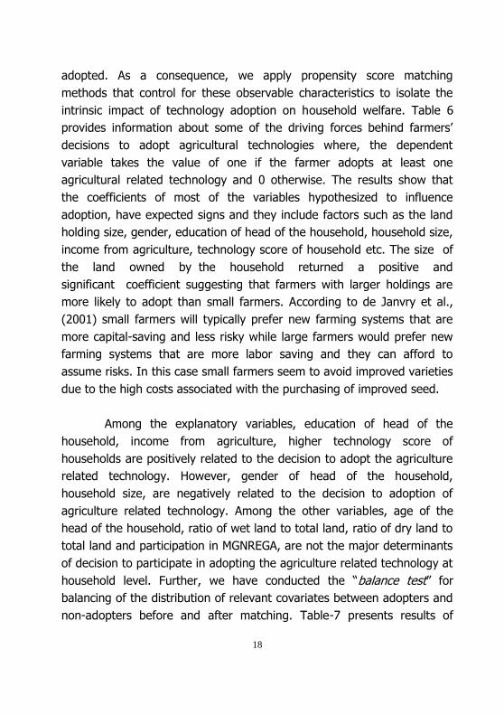
non-adopters before and after matching. Table-7 presents results of

19

propensity score matching quality indicators before and after matching.

The pseudo R2 also increased significantly from 48 percent before

matching to about 56 percent. This low pseudo R2, high total bias

reduction, and the significant p-values of the likelihood ratio test after

matching suggest that, the specification of the propensity is successful in

terms of balancing the distribution of covariates between the two groups.

Table 7: Adoption Effect on Per Capita Expenditure (Results

from the PSM) Matching algorithms NNMa NNMb KBMa KBMb

Pseudo R2 before matching 0.482 0.482 0.482 0.482

LR chi2 before matching 86.840*** 86.840*** 86.840*** 86.840***

Mean standardized bias before matching 21.157 21.157 21.157 21.157

Pseudo R2 after matching 0.561 0.543 0.541 0.541

LR chi2 after matching 87.531*** 89.541*** 88.651*** 88.567***

Mean standardized bias after matching 7.969 6.142 4.92 4.884

Total % bias reduction 62.329 71.678 76.797 76.989

Source: Primary data collected by authors during 2014 Note: *** indicate statistically 1% level; NNMa = single nearest neighbor matching with

replacement, common support, and caliper (0.03); NNMb = five nearest neighbors matching with replacement, common support, and caliper (0.03); KBMa = kernel based matching with band width 0.03, common support and KBMb = kernel based matching with band width 0.06, common support.

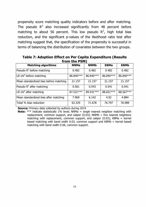
20

Table 8: Impact of Agricultural Related Technology Adoption

Matching algorithm Outcome (mean) ATT

Adopters Non-adopters

aNNM Per capita expenditure 9.582 9.381 0.200 (2.10)***

Head count ratio 0.586 0. 761 -0.174 (-2.67)***

Severity of poverty 0.529 0.513 -0.015

(0.10)

bNNM Per capita expenditure 9.582 9.414 0.167 (2.10)***

Head count ratio 0.586 0. 761 -0.129 (-2.29)***

Severity of poverty 0.529 0.509 0.020

(0.13)

aKBM Per capita expenditure 9.582 9.415 0.166 (2.23)***

Head count ratio 0.586 0.708 -0.121 (-2.20)***

Severity of poverty 0.529 0.519 0.009

(0.05)

bKBM Per capita expenditure 9.582 9.415 0.166 (2.29)***

Head count ratio 0.586 0.709 -0.122

(-2.25)***

Severity of poverty 0.529 0.523 0.006

(0.03) Source: Primary data collected by authors during 2014

Note: *** indicates statistical significance at the 1%. T-statistics in parenthesis, aNNM =

single nearest neighbor matching with replacement, common support, and caliper

(0.03); bNNM = five nearest neighbors matching with replacement, common

support, and caliper (0.03); aKBM = kernel based matching with band width 0.03,

common support and bKBM = kernel based matching with band width 0.06,

common support, Figures in parentheses at t-values

Table 8 reports the estimates of the average adoption effects

estimated using nearest neighbor matching (NNM) and kernel based

matching (KBM) methods. All the analyses were based on implementation

21

of common support and caliper, so that the distributions of adopters and

non-adopters were located in the same domain. As suggested by

Rosenbaum and Rubin (1985), we used a caliper size of one-quarter of

the standard deviation of the propensity scores. Three outcome variables

are used in the analysis such as (1) per capita expenditure, (2) head

count ratio, (3) severity of poverty index. The results indicate that,

adoption of agriculture related technologies have positive and significant

effect on per capita consumption expenditure and negative impact on

poverty.

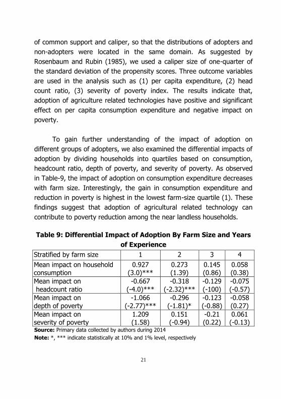
To gain further understanding of the impact of adoption on

different groups of adopters, we also examined the differential impacts of

adoption by dividing households into quartiles based on consumption,

headcount ratio, depth of poverty, and severity of poverty. As observed

in Table-9, the impact of adoption on consumption expenditure decreases

with farm size. Interestingly, the gain in consumption expenditure and

reduction in poverty is highest in the lowest farm-size quartile (1). These

findings suggest that adoption of agricultural related technology can

contribute to poverty reduction among the near landless households.

Table 9: Differential Impact of Adoption By Farm Size and Years

of Experience

Stratified by farm size (quartiles)

1 2 3 4

Mean impact on household consumption

0.927 (3.0)***

0.273 (1.39)

0.145 (0.86)

0.058 (0.38)

Mean impact on

headcount ratio

-0.667

(-4.0)***

-0.318

(-2.32)***

-0.129

(-100)

-0.075

(-0.57)

Mean impact on

depth of poverty

-1.066

(-2.77)***

-0.296

(-1.81)*

-0.123

(-0.88)

-0.058

(0.27)

Mean impact on severity of poverty

1.209 (1.58)

0.151 (-0.94)

-0.21 (0.22)

0.061 (-0.13)

Source: Primary data collected by authors during 2014

Note: *, *** indicate statistically at 10% and 1% level, respectively

22

CONCLUSION AND POLICY IMPLICATIONS

The relationship between agricultural technology adoption and welfare is

assumed to be straight forward. However, quantifying the causal effect of

technology adoption can be quite complex. This paper provides an ex-

post assessment of the impact of adoption of agricultural related

technology on per capita consumption expenditure and poverty status

measured by headcount index in rural India. Our results show that

adoption has a positive impact on consumption expenditures and

negative on poverty reduction. Though there is a large scope for boosting

the role of agricultural technology in anti-poverty policies in rural areas.

Implementing poverty alleviation measures, though, is not just the nature

of technology but also the inclusion of a poverty dimension into the

agricultural research priority-setting. Better targeting of agricultural

research on resource-poor producers might be the main vehicle for

maximizing direct poverty-alleviation effects. Improved agricultural

technology diffusion seems the most effective means of improving

agricultural productivity vis-à-vis reducing poverty. Improved rural

infrastructure, improved irrigation systems, maintenance of livestock,

physical assets, better access to education, secure land tenure, and

reasonable access to extension services all play a significant role in

encouraging productivity growth and poverty reduction. Technology

adoption, however, is constrained by lack of development of market

infrastructure, information asymmetry and agriculture extension services.

Policies that address these constraints and strengthen local institutions to

collectively improve access to technology, credit, and information will

increase both the spread and intensity of adoption.

23

REFERENCES

Ali, A. and A. Abdulai (2010), “The Adoption of Genetically Modified

Cotton and Poverty Reduction in Pakistan”, Journal of Agricultural

Economics, 61(1), pp. 175-192.

Becerril, J. and A. Abdulai (2010), “The Impact of Improved Maize

Varieties on Poverty in Mexico: A Propensity Score-Matching

Approach”, World Development, 38(7), pp. 1024-1035.

Bellon, M. R., M. Adato, J. Becerril and D. Mindek (2006), “Poor Farmers‟

Perceived Benefits from Different Types of Maize Germplasm:

The Case of Creolization in Lowland Tropical Mexico”, World

Development, 34(1), pp. 113-129.

Binswanger, H. P. and J. Von Braun (1991), “Technological Change and

Commercialization in Agriculture: The Effect on the Poor”, The

World Bank Research Observer, 6(1), pp. 57-80.

David, C. C. and K. Otsuka (Eds.) (1994), “Modern Rice Technology and

Income Distribution in Asia”, Int. Rice Res. Inst.

de Janvry, A. and E. Sadoulet (2002), “World Poverty and the Role of

Agricultural Technology: Direct and Indirect Effects”, Journal of

Development Studies, 38(4), pp.1-26.

de Janvry, A., G. Graff, E. Sadoulet and D. Zilberman (2001),

“Technological Change in Agriculture and Poverty Reduction”,

Concept Paper for the WDR on Poverty and Development.

Evenson, R. and D. Gollin (2003), “Assessing the Impact of the Green

Revolution: 1960 to 2000”, Science, 300(2), pp.758-762.

Foster, J., J. Greer and E. Thorbecke (1984), “A Class of Decomposable

Poverty Measures” Econometrica, 52(3), pp. 761-766.

24

Imbens, G. W. and J. D. Angrist (1994), “Identification and Estimation of

Local Average Treatment Effects”, Econometrica, 62, pp. 467-

476.

Just, R. E. and D. Zilberman (1988), “The Effects of Agricultural

Development Policies on Income Distribution and Technological

Change in Agriculture”, Journal of Development Economics, 28

(2), 193-216.

Karanja, D. D., M. Renkow and E. W. Crawford (2003), “Welfare Effects

of Maize Technologies in Marginal and High Potential Regions of

Kenya”, Agric Econ, 29(3), pp. 331-341.

Kassie, M., B. Shiferaw and G. Muricho (2011), “Agricultural Technology,

Crop Income, and Poverty Alleviation in Uganda”, World

Development, 39(10), pp. 1784-1795.

Kijima, Y., K. Otsuka and D. Sserunkuuma (2008), “Assessing the Impact

of NERICA on Income and Poverty in Central and Western

Uganda”, Agricultural Economics, 38(3), pp. 327-337.

Lee, M. J. (2005), “Micro-Econometrics for Policy, Program and

Treatment Effects”, Advanced Texts in Econometrics, Oxford

University Press.

Mendola, M. (2007), “Agricultural Technology Adoption and Poverty

Reduction: A Propensity Score Matching Analysis for Rural

Bangladesh”, Food Policy, 32(3), pp. 372-393.

Minten, B. and C. B. Barrett (2008), “Agricultural Technology,

Productivity, and Poverty in Madagascar”, World Development,

36(5), pp. 797-822.

25

Moyo, S., G. W. Norton, J. Alwang, I. Rhinehart and M. C. Demo (2007),

“Peanut Research and Poverty Reduction: Impacts of Variety

Improvement to Control Peanut Viruses in Uganda”, American

Journal of Agricultural Economics, 89(2), pp. 448-460.

Mwabu, G., W. Mwangi and H. Nyangito (2006), “Does Adoption of

Improved Maize Varieties Reduce Poverty? Evidence from

Kenya”, Paper Presented at the International Association of

Agricultural Economists Conference, Gold Coast, Australia.

Rangarajan, C. (2014), “Report of the Expert Group to Review the

Methodology for Measurement of Poverty”, Government of India,

Planning Commission, available at http://planningcommission.

nic.in/reports/genrep/pov_rep0707.pdf.

Rosenbaum, P. R. and D. B. Rubin (1985), “Constructing a Control Group

Using Multivariate Matched Sampling Methods that Incorporate

the Propensity Score”, American Statistician, 39(1), pp. 33-38.

Rubin, D. B. (1978), “Bayesian Inference for Causal Effects: The Role of

Randomization”, Annals of Statistics, 6, pp. 34-58.

Sianesi, B. (2004), “An Evaluation of the Swedish System of Active

Labour Market Programmes in the 1990s”, Review of Economics

and Statistics, 86(1), pp. 133-155.

Winters, P., A. de Janvry, E. Saudolet and K. Stamoulis (1998), “The Role

of Agriculture in Economic Development: Visible and Invisible

Surplus Transfers”, Journal of Development Studies, 345, pp. 71-

97.

Wu, H., S. Ding, S. Pandey and D. Tao (2010), “Assessing the Impact of

Agricultural Technology Adoption on Farmers‟ Well-being Using

Propensity Score Matching Analysis in Rural China”, Asian

Economic Journal, 24(2), pp. 141-160.

MSE Monographs

* Monograph 22/2012A Macro-Fiscal Modeling Framework for forecasting and Policy SimulationsD.K. Srivastava, K. R. Shanmugam and C.Bhujanga Rao

* Monograph 23/2012Green Economy – Indian PerspectiveK.S. Kavikumar, Ramprasad Sengupta, Maria Saleth, K.R.Ashok and R.Balasubramanian

* Monograph 24/2013Estimation and Forecast of Wood Demand and Supply in TamilanduK.S. Kavi Kumar, Brinda Viswanathan and Zareena Begum I

* Monograph 25/2013Enumeration of Crafts Persons in IndiaBrinda Viswanathan

* Monograph 26/2013Medical Tourism in India: Progress, Opportunities and ChallengesK.R.Shanmugam

* Monograph 27/2014Appraisal of Priority Sector Lending by Commercial Banks in IndiaC. Bhujanga Rao

* Monograph 28/2014Fiscal Instruments for Climate Friendly Industrial Development in Tamil NaduD.K. Srivastava, K.R. Shanmugam, K.S. Kavi Kumar and Madhuri Saripalle

* Monograph 29/2014Prevalence of Undernutrition and Evidence on Interventions: Challenges for IndiaBrinda Viswanathan.

* Monograph 30/2014Counting The Poor: Measurement And Other IssuesC. Rangarajan and S. Mahendra Dev

* Monograph 31/2015

Technology and Economy for National Development: Technology Leads to Nonlinear Growth

Dr. A. P. J. Abdul Kalam, Former President of India

* Monograph 32/2015

India and the International Financial System

Raghuram Rajan

* Mongraph 33/2015

Fourteenth Finance Commission: Continuity, Change and Way Forward

Y.V. Reddy

Santosh K. SahuSukanya Das

MADRAS SCHOOL OF ECONOMICSGandhi Mandapam Road

Chennai 600 025 India

October 2015

IMPACT OF AGRICULTURAL RELATED TECHNOLOGY ADOPTION ON POVERTY:

A STUDY OF SELECT HOUSEHOLDS IN RURAL INDIA

MSE Working Papers

Recent Issues

* Working Paper 120/2015Health Shocks and Coping Strategies: State Health Insurance Scheme of Andhra Pradesh, IndiaSowmya Dhanaraj

* Working Paper 121/2015Efficiency in Education Sector: A Case of Rajasthan State (India)Brijesh C Purohit

* Working Paper 122/2015Mergers and Acquisitions in the Indian Pharmaceutical SectorSantosh Kumar Sahu and Nitika Agarwal

* Working Paper 123/2015Analyzing the Water Footprint of Indian Dairy IndustryZareena B. Irfan and Mohana Mondal

* Working Paper 124/2015Recreational Value of Coastal and Marine Ecosystems in India: A Partial EstimatePranab Mukhopadhyay and Vanessa Da Costa

* Working Paper 125/2015Effect of Macroeconomic News Releases on Bond Yields in India China and JapanSreejata Banerjee and Divya Sinha

* Working Paper 126/2015Investigating Household Preferences for Restoring Pallikaranai MarshSuganya Balakumar and Sukanya Das

* Working Paper 127/2015The Culmination of the MDG's: A New Arena of the Sustainable Development GoalsZareena B. Irfan, Arpita Nehra and Mohana Mondal

* Working Paper 128/2015Analyzing the Aid Effectiveness on the Living Standard: A Check-Up on South East Asian CountriesZareena B. Irfan, Arpita Nehra and Mohana Mondal

* Working Paper 129/2015Related Party Transactions And Stock Price Crash Risk: Evidence From IndiaEkta Selarka and Subhra Choudhuryana Mondal

* Working Paper 130/2015Women on Board and Performance of Family Firms: Evidence from India Jayati Sarkar and Ekta Selarka

* Working papers are downloadable from MSE website http://www.mse.ac.in

$ Restricted circulation

WORKING PAPER 131/2015