implementation and analysis of a clothoid-based model...

I ,EXAMENSARBETE SYSTEMTEKNIK OCH ROBOTIK 120 HPAVANCERAD NIVÅ

, STOCKHOLM SVERIGE 2015

Implementation and Analysis of aClothoid-based Model PredictiveController

TEDDY JUHLIN-HENRICSON

KTH KUNGLIGA TEKNISKA HÖGSKOLAN

SKOLAN FÖR ELEKTRO- OCH SYSTEMTEKNIK

Abstract

For the last couple of years autonomous driving has increased in popularity as a researcharea, and it continues to grow. A topic within autonomous driving is path following, whichis the subject studied in this project. One of the popular controllers to use for controlling avehicle is the model predictive controller, because it finds an optimal control input for thevehicle based on the model of the vehicle, and its estimated future behaviour within theprediction horizon - which covers a distance ahead of the vehicle. To increase the length ofthis distance, one can use a new controller - the clothoid-based model predictive controller.

The clothoid-based model predictive controller is a linear time-varying model predictivecontroller that uses a clothoid-based vehicle model to find an optimal input based onthe vehicle’s behaviour at the kink-points. The kink-points are way-points that are usedto create the clothoids, and the distance between them can be very far. Therefore, it ispossible to cover a large distance ahead of the vehicle with a small prediction horizon.

In this thesis, the controller is implemented at the Smart Mobility Laboratory at KTHRoyal Institute of Technology so that it can be tested and evaluated for future use. Thecontroller is implemented on a 1 : 32 scaled radio truck that is monitored by a motioncapture system, and remotely controlled by a desktop computer.

The outcome of the implementation is a new controller for the remote controlled radiotrucks with a fast control algorithm, where the greatest mean deviation from the path was0.117m.

2

Abstrakt

Under de senaste aren har sjalvkorande fordon blivit popularare som forskningsomrade, ochdet blir allt mer populart. Ett omrade inom sjalvkorande fordon ar att den ska folja efteren bana, aven kallat path following, vilket ar omradet som projektet fokuserat pa. En avde populara kontrollerna for att styra fordonet ar predikterande modell-kontroller (modelpredictive control), for den hittar en den optimala kontrol signalen baserat pa modellen avfordonet och dess framtida bettende inom prediktions horisonten - som tacker ett omradeframfor bilen. For att oka tackningsgraden av det har omradet kan en anvanda en nykontroller - den klotoidbaserade predikterande modell-kontroller (clothoid-based modelpredictive controller).

Den klotoidbaserade predikterande modell-kontroller ar en linjart tidsvarierande predik-terande modell-kontroller (linear time-varying model predictive controller) som anvandersig av en klotoidbaserad fordonsmodel for att hitta den optimala inputsignalen baseratpa fordonets beteende vid knut-punkterna (kink-points). Knut-punkterna ar punkter somanvands for att skapa klotoiderna, och avstandet mellan punkterna kan vara langt. Darforar det mojligt att tacka ett storre omrade framfor fordonet med en mindre prediktionshorisont.

I den har uppsatsen ar kontroller implementerad i Smart Mobility Laboratory paKungliga Tekniska Hogskolan, sa att den kan bli evaluerad och testad for anvandning iframtiden. Kontrollern anvands pa en 1 : 32 skalenlig radiostyd lastbild som ar overvakadav ett rorelse detektionssystem, och lastbilen ar radio fjarrstyrd via en dator.

Resultatet av implementeringen ar en ny kontroller for radiostyrd lastbil med en snabbkontroller algorithm med en maximal medelavvikelse fran banan pa 0.117m.

3

Table of Contents

Abstract 2

Abstrakt 3

1 Introduction 71.1 Background . . . . . . . . . . . . . . . . . . . . . . . . . . . . . . . . . . . . 7

1.1.1 Related work . . . . . . . . . . . . . . . . . . . . . . . . . . . . . . . 81.2 Problem Formulation . . . . . . . . . . . . . . . . . . . . . . . . . . . . . . 9

1.2.1 Hypothesis . . . . . . . . . . . . . . . . . . . . . . . . . . . . . . . . 91.3 Thesis Outline . . . . . . . . . . . . . . . . . . . . . . . . . . . . . . . . . . 9

2 Clothoid-based Model Predictive Controller 102.1 Clothoids . . . . . . . . . . . . . . . . . . . . . . . . . . . . . . . . . . . . . 102.2 Vehicle model . . . . . . . . . . . . . . . . . . . . . . . . . . . . . . . . . . . 112.3 Model Predictive Control . . . . . . . . . . . . . . . . . . . . . . . . . . . . 14

2.3.1 Reference Tracking . . . . . . . . . . . . . . . . . . . . . . . . . . . . 152.3.2 Linear Time Varying Model Predictive Control . . . . . . . . . . . . 162.3.3 Quadratic Programming Formulation . . . . . . . . . . . . . . . . . 162.3.4 Summary . . . . . . . . . . . . . . . . . . . . . . . . . . . . . . . . . 18

2.4 Clothoid-based Model Predictive Control . . . . . . . . . . . . . . . . . . . 182.4.1 The Algorithm . . . . . . . . . . . . . . . . . . . . . . . . . . . . . . 182.4.2 Vehicle’s Steering Angle and Path’s Curvature . . . . . . . . . . . . 18

3 Experimental Set-up 203.1 Test Paths . . . . . . . . . . . . . . . . . . . . . . . . . . . . . . . . . . . . 20

3.1.1 Path 1 - Straight Line . . . . . . . . . . . . . . . . . . . . . . . . . . 203.1.2 Path 2 - L-turn . . . . . . . . . . . . . . . . . . . . . . . . . . . . . . 203.1.3 Path 3 - C-turn . . . . . . . . . . . . . . . . . . . . . . . . . . . . . . 20

3.2 Test Scenarios . . . . . . . . . . . . . . . . . . . . . . . . . . . . . . . . . . 223.2.1 Scaled-Truck Starts On Path with No Disturbance . . . . . . . . . . 223.2.2 Scaled-Truck Starts On Path with Disturbance . . . . . . . . . . . . 223.2.3 Scaled-Truck Starts with an Offset to The Path with No Disturbance 223.2.4 Scaled-Truck Starts with an Offset to The Path with Disturbance . 22

3.3 Simulations . . . . . . . . . . . . . . . . . . . . . . . . . . . . . . . . . . . . 223.3.1 CVXGEN . . . . . . . . . . . . . . . . . . . . . . . . . . . . . . . . . 223.3.2 Simulation Algorithm . . . . . . . . . . . . . . . . . . . . . . . . . . 233.3.3 Scaled-Truck Modelling . . . . . . . . . . . . . . . . . . . . . . . . . 23

3.4 Experiments . . . . . . . . . . . . . . . . . . . . . . . . . . . . . . . . . . . . 273.4.1 Laboratory System . . . . . . . . . . . . . . . . . . . . . . . . . . . . 273.4.2 Experimental Evaluation . . . . . . . . . . . . . . . . . . . . . . . . 29

5

4 Results 304.1 Simulation Results . . . . . . . . . . . . . . . . . . . . . . . . . . . . . . . . 30

4.1.1 Sampling Time with No Disturbance . . . . . . . . . . . . . . . . . . 324.1.2 Sampling Time with Disturbance . . . . . . . . . . . . . . . . . . . . 364.1.3 Off-set Start Position of Path . . . . . . . . . . . . . . . . . . . . . . 404.1.4 Off-set Start Position of Path with Disturbance . . . . . . . . . . . . 434.1.5 Conclusion . . . . . . . . . . . . . . . . . . . . . . . . . . . . . . . . 46

4.2 Implementation Results . . . . . . . . . . . . . . . . . . . . . . . . . . . . . 474.2.1 Path 1 - Straight Line . . . . . . . . . . . . . . . . . . . . . . . . . . 474.2.2 Path 2 - Low Curvature Path . . . . . . . . . . . . . . . . . . . . . . 484.2.3 Path 3 - High Curvature Path . . . . . . . . . . . . . . . . . . . . . 494.2.4 Conclusion . . . . . . . . . . . . . . . . . . . . . . . . . . . . . . . . 50

5 Conclusions and Discussions 515.1 Conclusions . . . . . . . . . . . . . . . . . . . . . . . . . . . . . . . . . . . . 51

6 Future work 52

6

Chapter 1

Introduction

The master’s thesis covers an implementation of a clothoid-based model predictive controllerfor autonomous driving of a 1:32 scaled radio truck in the Smart Mobility Laboratory atthe Royal Institute of Technology, KTH.

1.1 Background

For years, self-going vehicles have only been a dream. During the last couple of decades,the dream comes closer to reality as technology is getting more advanced. New sensors,computers, and algorithms makes it possible to have self-driving vehicles, since they havebeen used to improve the driving experience, and safety of the vehicle with advanced driverassistance systems (ADAS) such as anti-lock braking systems (ABS), cruise control (CC),electronic stability control, and adaptive cruise control (ACC). These systems are greatsteps towards self-driving vehicles.

Autonomous driving vehicles are increasing in numbers, and some examples of con-tributing companies are Google, Mercedes-Benz, Scania, and Volvo, and universities allover the world such as the Royal Institute of Technology (KTH). KTH is part of an projecttogether with SAAB, Autoliv, Linkoping University, and Scania. The project is iQMatic,and it is led by Scania. The purpose of the project is to gain information and experienceabout autonomous vehicles and systems with the goal of having a fully autonomous HDVin 2016. Some examples of a first implementation of autonomous vehicles would be asan industrial application such as rock quarries, mine exploration, construction sites, orfactory environments. The reason behind this is that the vehicles are used within closedareas, and it is much easier to implement self-driving vehicles and systems in closed areascompared to public areas due to legal regulations.

A topic in autonomous driving is path following. Path following is to ensure that avehicle is actually performing the correct action to follow the given path to reach the goal.It is of high importance that the vehicle follows these orders since it can have devistatingresults if not. Therefore, once can use a predetermined path constituted by checkpointsthat is generated offline or online. Each checkpoint on the path contains the necessaryinformation and actions for the vehicle to move along the path. The information at thecheckpoints can be the position, speed and heading of the vehicle.

To help the politicians with their decisions, the engineers and scientists needs to findsolutions that are safe and reliable. A popular control algorithm is the model predictivecontrol, which uses a set of future points (prediction horizon), a model of the vehicle,constraints of the model, and an optimization problem to calculate an optimal input signalto control the vehicle. A common problem has been that the future points only representsa small distance ahead of the vehicle. Normally, the points are selected by multiplyingthe vehicle’s velocity with a small time period (the sampling time). As an example, let

7

a vehicle travel in 14m s�1 (about 50kmh�1) with a sampling time of 100ms, and using10 points in the prediction horizon will result in a distance of 14m ahead of the vehicle,which is not sufficient to control the vehicle in a reliable and safe matter when driving sofast. The prediction horizon can be increased, but this will increase the computationalpower and time. Therefore, if the distance between the points in the prediction horizonare increased, the prediction horizon covers a greater distance ahead of the car and thecontroller would be able to control the vehicle more reliable.

To increase the distance greatly, a controller that was introduced during the springof 2015 is the Clothoid-based Model Predictive Control (MPCC) by Lima, et al. in [1]from KTH. The controller is based on a linear time-varying model predictive control(LTV-MPC), and the similarities between a vehicle’s steering and clothoids. As will beexplained for the reader further in the thesis or as in [1], the clothoid-based model predictivecontrol’s prediction horizon is able to cover great distances ahead of the vehicle due to theproperties of creating clothoids, the kink-points.

The next step would be to test it on real vehicles, but before applying it on real sizedvehicles, it can be implemented in a laboratory at KTH - the Smart Mobility Laboratory,where the controller can be implemented, tested, and evaluated for 1 : 32 scaled radiotrucks before implementing the controller for controlling real vehicles.

1.1.1 Related work

The number of contributions of autonomous driving has increased largely the last coupleof decades, and one of the most popular controllers to control the vehicle is the modelpredictive control. It uses a model of the real vehicle for predicting its behaviour so that itfinds an optimal input sequence by solving an optimization problem with a cost function,and then the input is applied to the vehicle [2].

In [3], the authors have approached a path following problem with the use os a fourwheel vehicle model and non-linear tire model together with a LTV-MPC that is used forcontrolling said vehicle for active front steering, braking and differentials. The LTV-MPCuses a linear time-varying system that is created by linearizing the non-linear modelsaround the current state and the previous control input. The LTV-MPC is then formulatedas a convex quadratic programming (QP) problem, such that it can control the front wheelssteering angle and the slip ratio for the four wheels to follow the desired path while thelongitudinal speed is kept close to the reference. The controller is evaluated in simulationsby letting the vehicle perform a double lane change on a snow covered road. The resultsshows an overall good tracking of the desired path when the longitudinal speed is weightedusing a small weight and a long prediction horizon, because it was allowed to drasticallylower the speed of the vehicle before the curve.

Another contribution to autonomous driving with MPC is a robot vehicle for trajectorytracking [4]. To solve the trajectory tracking problem, they used two approaches. Thefirst is a non-linear MPC and the other is a linear MPC formulated as a QP problem. Therobot is modelled with a kinematic vehicle model with the linear and angular velocities asthe control inputs. The linear MPC successively linearizes the model around the referenceinputs and states, to obtain a LTV system. The results of the simulations shows thatthere is no significant difference between the non-linear and linear MPC for the trajectorytracking, but the computational effort is lower when formulating the linear MPC on QPform compared to the non-linear MPC.

The main related work for the MPCC implementation is [1] for the controller itself,and [5] together with [6] for the thorough explanations of the system in the Smart MobilityLaboratory. The system in the Smart Mobility Laboratory is containing the Qualisysmotion capture system, PCs, and 1 : 32 scaled radio trucks.

In [1], the authors present the novel MPCC which combines the theory of clothoids

8

with model predictive control for a path following problem. The approach of solving thepath following problem has been to formulate the MPC controller based on the fact thatthe path of a vehicle travelling at low speeds defines a segment of clothoids if the steeringangle is limited to vary piecewise linearly. This makes it possible to comput the vehiclemotion as clothoids parameters and translate them to vehicle inputs. The results of thesimulations shows a short prediction horizon that covers an average distance of 180mwhen the vehicle travels with a constant velocity of 10m s�1 and the MPC solution isrecomputed each 0.01s. Compared to the LTV-MPC, as the authors have done, the MPCC(or LTV-MPCC) is achieving a smoother and more comfortable driving while remainingalmost the same path following accuracy.

1.2 Problem Formulation

The clothoid-based model predictive controller (MPCC) introduced in [1] is implementedin the Smart Mobility Laboratory (SML) at KTH for a 1 : 32 scaled mini-truck. Theresults of the controller’s performance are the time it takes to run the controller algorithm,and the mean and maximum deviation. These results can be defined as the set of criteriato evaluate the implementation of the controller in SML.

1.2.1 Hypothesis

Can a Clothoid-based Model Predictive Controller be used to control a mini-truck with the motion capture system in the Smart Mobility Laboratory, withrespect to the set of criteria?

The set of criteria is the controller’s performance, a mini-truck is a 1 : 32 scaledradio car version of a Scania R620 Topline truck, and the motion capture system isfrom Qualisys.

1.3 Thesis Outline

The rest of the thesis is outlined as followed: Chapter 2 describes the clothoid-based modelpredictive controller from a theoretical point of view. Chapter 3 adress the simulation andexperimental setup, respectively. The results are presented, and discussed in chapters 4and 5. Last, in chapter 6 is suggestions of future work for the controller, and more.

9

Chapter 2

Clothoid-based Model PredictiveController

2.1 Clothoids

Clothoids are spirals where the curvature is changing linearly with the travelled distance,the arc-length. This creates a smooth transition. The change of the curvature reducesthe lateral acceleration of the vehicle which occurs when a vehicle turns [7], and thereforeprovides a comfortable experience for the passengers. Clothoids are also known as spiros,Euler spirals or Conu spirals.

When a vehicle is travelling along a straight road, and the road suddenly turns, thevehicle experiences a centrifugal acceleration. This sudden acceleration instantly causesjerk, increasing the lateral acceleration and discomfort for the passengers. To prevent thisfrom happening, roads are generally designed using clothoids.

Mathematically, a clothoid is defined by the Fresnel integrals [7], which is representedas

x(L) =

ZL

0cos(s2/2)ds (2.1a)

y(L) =

ZL

0sin(s2/2)ds, (2.1b)

where L 2 R is the clothoid’s arc-length, and s2/2 is the angle of tangent. An example ofclothoids is presented in Fig. 2.1, with positive (L � 0) and negative (L 0) arc-length.

Next, let us find a relationship between the clothoid’s angle of tangent, and thecurvature of the clothoid. Consider a circle with radius R, with two points A and B, anangle �✓, and an arc-length �s between these points, as shown in Fig. 2.2.The definition of an arc-length between two points on a circle is defined as

�s = R�✓,

and with some algebraic maniupulations, we get

�✓

�s=

1

R. (2.2)

In [8, p. 89], Augustin-Louis Cauchy defines the curvature as the reciprocal of theradius of a circle, = R�1, and as the points A and B gets closer to each other, � becomesinfinitesimal, and (2.2) can be rewritten as

10

�1 0 1

�1

0

1

Arc-length, Asymptotic point.

Figure 2.1

O

A

B

�s

�✓

Figure 2.2: The black line is the circle with radius R where two points A, and B definesan arc-length �s, which is the solid cyan arc, and angle �✓ which is defined by OAB.

d✓

ds= . (2.3)

This means that the curvature of a curve is defined as the rate of change of the angle ✓that its tangent makes with the x-axis, and the relationship between the tangent’s angleand the curvature is found.

2.2 Vehicle model

The implementation is done in a 1:32 scaled radio truck, and in order to control it, a modelis needed. Since the radio truck is scaled down by 32 of a real truck, it is possible toassume that there is no wheel slip, and it is moving at low speeds - up to 0.7m s�1 [9] sothe lateral acceleration have no influence on the vehicle, and can be neglected. Thereforeit is possible to discribe the motion of the vehicle using a kinematic model.

A car-like model is illustrated in Fig. 2.3. In [10], a simplified model is presented. By

11

assuming that the two wheels in the front are merged into one wheel, and the same for thewheels on the back wheelbase, as in the left figure in Fig. 2.3. This is a 2-wheel model,called a bicycle model.

�

�

D

✓

Front Wheels, Back Wheels,Vehicle Body, Front Wheels’ Angle, Vehicle’s Orientation.

�

D

✓

y

x

y

x

Bicycle Model

Figure 2.3

With the help of Fig. 2.3, the kinematic model can now be defined as

dx(t)

dt= v(t) cos (✓(t)) , (2.4a)

dy(t)

dt= v(t) sin (✓(t)) , (2.4b)

d✓(t)

dt=

v(t)

Dtan (�(t)) . (2.4c)

Where x and y are the coordinates of the vehicles position in a global coordinate system, ✓is the vehicles yaw angle, D is the wheelbase distance, v is the longitudinal speed and � isthe steering angle of the front wheels.

Recall the road design method presented in Section 2.1. An advantage of using theclothoid as a representation of a curve, is that it represents the motion of a vehicle inspace-domain, when the steering angle of a vehicle is limited to vary linearly, and usea constant velocity of the vehicle. Therefore, we can translate (2.4) to space-domain bymaking v(t) · dt = ds, and assuming that v(t) 6= 0 and v(t) is a continuous function, suchthat

dx(s)

ds= cos (✓(s)) (2.5a)

dy(s)

ds= sin (✓(s)) (2.5b)

d✓(s)

ds=

1

Dtan (�(s)) , (2.5c)

is the vehicle model in space-domain.We know that d✓(s)

ds

= (s), where (s) is the curvature of a clothoid, and since theclothoid is describing the motion of a vehicle, it will also be the curvature of the vehilce. Bylimiting the steering angle to vary linearly with a piecewise linear function, the motion ofthe vehicle is discribed as a segment of a clothoid where the curvature is also limited with

12

a piecewise linear function. The change of the curvature is then a constant, as d(s)ds

= c,where c is the curvature sharpness.

If the path is represented by N � 1 clothoid segments which are described by Nkink-points, it is possible to build paths as presented in Fig. 2.4. The kink-points works aswaypoints, and we can reconstruct the path only with the information contained in thekink-points.

0 1 2 3 4 5 6 70

1

2

3

x [m]

y[m

]

0 1 2 3 4 5 6 7 8 9

�2

0

2

4

Distance travelled [m]

Curvature

[m-1]

Path, Kink-points.

Figure 2.4

The state of the vehicle at each kink-point is defined as z(si

) = zi

= [xi

, yi

, ✓i

,i

]T , andinput as u(s

i

) = ui

= [ci

, Li

]T , where ci

and Li

are the i-th clothoid curvature sharpness(which is constant by definition) and arc-length respectively. Then using (2.5) and thefact that (s) is a piecewise linear function, the vehicle state evolution at each kink-pointis computed using the discrete function f(z

i

,ui

), defined as

xi+1 = x

i

+

Zsi+1

si

cos

✓✓i

+ i

(s� si

) + ci

(s� si

)2

2

◆ds, (2.6a)

yi+1 = y

i

+

Zsi+1

si

sin

✓✓i

+ i

(s� si

) + ci

(s� si

)2

2

◆ds, (2.6b)

✓i+1 = ✓

i

+ i

Li

+ ci

L2i

2, (2.6c)

i+1 =

i

+ ci

Li

, (2.6d)

where i = 1, ..., N . As we can see, the integrals in (2.6a) and (2.6b) are the FresnelIntegrals, and they do not have an explicit solution. Therefore, by approximating theseintegrals with Riemann sums so that the integrals are substituted with their correspondingarc-lengths, so that we get

13

xi+1 = x

i

+ Li

cos

✓✓i

+ i

Li

+ ci

L2i

2

◆, (2.7a)

yi+1 = y

i

+ Li

sin

✓✓i

+ i

Li

+ ci

L2i

2

◆, (2.7b)

✓i+1 = ✓

i

+ i

Li

+ ci

L2i

2, (2.7c)

i+1 =

i

+ ci

Li

, (2.7d)

which is the final form for the clothoid-based vehicle model in space-domain.

2.3 Model Predictive Control

Model predictive control (MPC) is a multi-variable optimal control algorithm. It usesan optimization problem with a model of the system to predict the behaviour of it, andconstraints of the system during a set of time steps ahead in time - the prediction horizon.The controller finds an optimal input sequence within the prediction horizon, and appliesthe first control input to the system. The horizon is shifted forward, and the process isrepeated. The shifting of the horizon in the controller, and one step of the process isillustrated in Fig. 2.5.

past future

horizon

Ts Ts + 1 · · · · · · · · · · · · ·Ts +N

Input prediction

reference

U

⇤[Ts]u

⇤[Ts]

Output prediction

Ts + 1 Ts + 2 · · · · · · · · · · · · ·Ts + 1 +N

Input prediction

reference

U

⇤[Ts]u

⇤[Ts]

Output prediction

Figure 2.5

The optimal control problem is an optimisation problem with a cost function, C subjectto constrains which usually are the system model and the limitations of the system. Ingeneral, the system model is non-linear or a linearisation of a non-linear model so that it isan approximated linear model. The constraints can be physical limitation of the system.A general set-up of the optimization problem can be found in (2.8).

14

U⇤ 4=minimize

z,u

NX

1

C (zi

,ui

) (2.8a)

subject to zi+1 = f(z

i

,ui

), (2.8b)

zi

2 Z (2.8c)

ui

2 U (2.8d)

where C is the cost function, N denotes the finite horizon, zi

is the system states, ui

is thesystem inputs, z

i+1 = f(zi

,ui

) denotes the system model, Z,U describes the constraints ofthe system states and inputs, and U⇤ denotes the solution to the optimization system, i.e.the optimal input sequence.

2.3.1 Reference Tracking

A fundamental objective of control is to ensure a system follows a reference by minimizingthe difference to the systems output, for example: the illustration in Fig. 2.5 shows areference tracking, which could represent a system which is following a path. Therefore,we need to do a small, but important, modification of the MPC formulation. The theorycan be found in [2], but an explanation of the fundamental thinking and modifications willbe presented below.

The first modifications to do is in the cost function. In order to reduce the computationalburden of an optimisation problem, it can be defined as a convex optimisation problem.In [11], it is shown that convex optimisation problems are reliable and efficient solved, andsuitable for automatic control such as MPC. For the optimization problem to be convex,the cost function and the constraints need to belong to convex sets. Some examples:the functions of lines, quadratic functions, hyperplanes and norms. We kindly refer thereader who is interested in convex optimization to [11]. Therefore, the cost function canbe formulated as a quadratic function,

C4= zT

N

Qf

zN

+N�1X

1

�zTi

Qi

zi

+ uT

i

Ri

ui

�, (2.9)

where Qi

⌫ 0 and Ri

⌫ 0 which are weight matrices and Qf

⌫ 0 is a weight matrix forthe final state in the horizon.

Second, as the cost function is in its current form, the system will reach the origin ifthe solution converges, and the origin is a steady state of the system. The steady statecan be refereed to as zref

i

with uref

i

as the steady state input. The new formulation of thecost function (2.9) is then

(zN

�zrefN

)TQf

(zN

�zrefN

)+N�1X

1

⇣(z

i

� zrefi

)TQi

(zi

� zrefi

) + (ui

� uref

i

)TRi

(ui

� uref

i

)⌘.

Let zi

= zi

� zrefi

and ui

= ui

� uref

i

, 8i = 1, ..., N and the cost function can berewritten as

C = zTN

Qf

zN

+N�1X

1

�zTi

Qi

zi

+ uT

i

Ri

ui

�. (2.10)

Now it is possible to see the steady state as a reference point, which will make thesystem follow a reference. The reference can now be points on a path, and we have achieveda path following formulation for MPC.

15

2.3.2 Linear Time Varying Model Predictive Control

In the section 2.2 the presented models have non-linear characteristics because of thetrigonometric functions. If the model would be used in its current form, the MPC wouldbe solving a non-linear optimization problem which has a huge computational burden.To decrease the computational burden, it is possible to linearise the model along thereference path to get a linear approximation of the model, and this gives us a linear timevarying MPC [12]. The linearisation can be computed on- or off-line, and to reduce thecomputational burden for on-line computing, the linearisation is done off-line.

Linearisation

Let f(zi

,ui

) be a non-linear system with zi

as states and ui

as inputs of a system atsample time i. The linearisation of a non-linear system, f(z

i

,ui

), is defined as the Jacobianmatrices of f(z

i

,ui

) w.r.t. the variables zi

and ui

,

Ai

=@f(z

i

,ui

)

@zi

��(zrefi ,uref

i )

=

2

64

@f1@z1

· · · @f1@zn

.... . .

...@fm@z1

· · · @fm@zn

3

75

��(zrefi ,uref

i )

Bi

=@f(z

i

,ui

)

@ui

��(zrefi ,uref

i )

=

2

64

@f1@u1

· · · @f1@ul

.... . .

...@fm@u1

· · · @fm@ul

3

75

��(zrefi ,uref

i )

,

(2.11)

where n, m, l are the degrees of freedom for the system states, non-linear system andsystem inputs respectively.

This operation is then applied at each point and/or sampling time on the trajectory ofthe nonlinear system f(z

i

,ui

).The linear approximation of the non-linear system is then

zi+1 = A

i

zi

+Bi

ui

, i = 1, ..., N, (2.12)

where zi

and ui

is the linear approximation of the systems states and inputs respectively,A

i

and Bi

are the linearisation matrices of the non-linear system f(zi

,ui

) from (2.11).

2.3.3 Quadratic Programming Formulation

Quadratic programming formulation (QP-form) is used for faster computation of convexoptimization problems, and it is possible to transform the LTV-MPC explained in Sec-tion 2.3.2. To find the QP-form of the LTV-MPC, let us start with how the system stateszi

evolves at each iteration.

zi+1 = A

i

zi

+Bi

ui

zi+2 = A

i+1zi+1 +Bi+1ui+1 = A

i+1 (Ai

zi

+Bi

ui

) +Bi+1ui+1 =

= Ai+1Ai

zi

+Ai+1Bi

ui

+Bi+1ui+1

zi+3 = A

i+2zi+2 +Bi+2ui+2 = . . . =

= Ai+2Ai+1Ai

zi

+Ai+2Ai+1Bi

ui

+Ai+2Bi+1ui+1 +B

i+2ui+2

...

zi+n

= . . . = Ai+n�1Ai+n�2 · · ·Ai+1Ai

zi

+Ai+n�1Ai+n�2 · · ·Ai+1Bi

ui

+ . . .

. . .+Ai+n�1Bi+n�2ui+n�2 +B

i+n�1ui+n�1,

(2.13)

16

which leads us to introduce the following vectors:

Zi+1 =

2

664

zi+1

zi+2

...zi+n�1

zi+n

3

775, Ui

=

2

664

uiui+1

...ui+n�2

ui+n�1

3

775. (2.14)

In (2.13), we can see that all the states are dependent only on the first state z1, butall the inputs for i = 1, ..., n � 1, which is seen in the last state z

n

. Then the matrixrepresentation of the equations in (2.13) is

Ai

=

2

66666664

Ai

Ai+1Ai

Ai+2Ai+1Ai

...A

i+n�2Ai+n�3 · · ·Ai+1Ai

Ai+n�1Ai+n�2 · · ·Ai+1Ai

3

77777775

(2.15a)

Bi

=

2

66666664

Bi

0 0 . . . 0A

i+1Bi

Bi+1 0 . . . 0

Ai+2Ai+1Bi

Ai+2Bi+1 B

i+2 . . . 0...

...... . . .

...A

i+n�2Ai+n�3 · · ·Ai+1Bi

Ai+n�2 · · ·Ai+2Bi+1 A

i+n�2 · · ·Ai+3Bi+2 . . . 0A

i+n�1Ai+n�2 · · ·Ai+1Bi

Ai+n�1 · · ·Ai+2Bi+1 A

i+n�1 · · ·Ai+3Bi+2 . . . Bi+n�1

3

77777775

(2.15b)

Combining (2.14) with (2.15) we can rewrite (2.13) in matrix form.

Zi+1 = A

i

zi

+ Bi

Ui

(2.16)

Doing the same for the quadratic cost function from (2.10), and combining with (2.15)we get the quadratic cost function in matrix form,

Ci

= ZT

i+1QZi+1 + UT

i

RUi

, (2.17)

where

Q = diag(Q,Q, ...,Qf

), R = diag(R,R, ...,Rf

)

where Q 2 Rn⇥n, Qf

2 Rn⇥n, and R 2 Rl⇥l such that Q 2 Rn·N⇥n·N and R 2 Rl·N⇥l·N

where N is the horizon window, n the number of states, and l is the number of input.Replacing Z

i+1 with the right hand side of (2.16), the cost function (2.17) can bewritten as:

Ci

=1

2UT

i

Hi

Ui

+ fTi

Ui

+ di

, (2.18)

with

Hi

= 2(BT

i

Qi

Bi

+ Ri

), (2.19a)

fi

= 2Bi

Qi

Ai

z1, (2.19b)

di

= zT1 AT

i

Qi

Ai

z1, (2.19c)

17

2.3.4 Summary

We can finally present the LTV-MPC formulation for path following

U⇤ 4=minimize

Ui

1

2UT

i

Hi

Ui

+ fTi

Ui

(2.20a)

subject to

I�I

�U

i

"uMAX

� uref

i

uMIN

+ uref

i

#(2.20b)

(2.20c)

where U⇤ is the optimal input sequence for the system, uMAX

and uMIN

are the inputconstraints, uref

i

are the input references, Hi

and fi

are defined in (2.19) and Ui

is thevector form of the inputs of the prediction horizon.

2.4 Clothoid-based Model Predictive Control

One great challenge of using a MPC for a vehicle while following a path in real-life is thatthe distance of the prediction horizon needs to be sufficient long ahead of the vehicle, andthe number of points in the horizon needs to be sufficient small such that the MPC can besolved within the available computation time. There is a trade-off between the number ofpoints in the horizon, and the computation time for the optimisation problem to be solved.

One solution is to use the clothoid-based vehicle model with kink-points presentedin Section 2.2 due to the advantage of building big paths with few way-points. Usingthis clothoid model as the system and only the kink-points as reference points meansthat an MPC as in Section 2.3 can use a small prediction horizon (N < 10), and stillpredict the vehicles behaviour far ahead on the path. This combination is what defines theclothoid-based model predictive control (MPCC) [1].

The key factor in MPCC is that it only uses the references at the kink-points. Thenobtaining the optimal input signal from the MPCC, it is possible to manipulate the optimalinput such that it can be applied to a kinematic vehicle model because of the similaritiesto the clothoid model, as mentioned in section 2.2.

2.4.1 The Algorithm

The main challenge in using MPCC is finding the reference points, which are the closestpoint on the path, and the kink-points ahead of that point. Once those are found, it is justan LTV-MPC in QP-formulation with the clothoid-based vehicle model as the internalmodel. The algorithm of MPCC is presented in Algorithm 2.1.

2.4.2 Vehicle’s Steering Angle and Path’s Curvature

The optimal input calculated by MPCC is used in the clothoid model in (2.7). The inputsare the curvature sharpness c and arc-length L. The inputs for the vehicle model (2.4) arethe velocity v and steering angle �. To control the orientation of the vehicle, a relationbetween the steering angle and the curvature sharpness, i.e. � and c, is needed to be found.Therefore, by combining (2.5c) with (2.5c), we can find a relation between the vehicle’ssteering angle, and its curvature. Hence,

=1

Dtan(�) =) � = arctan(D) (2.21)

where is the curvature of the clothoid model, � is the steering angle of the vehicle and Dis the length between the wheelbases.

18

Algorithm 2.1 MPCC Algorithm, MPCC Alg

1: function FindReferences(zvehiclei

)2: refPos ClosestPointOnPath ReferenceF inder(zvehicle

i

)3: refKink Kinkpoints ReferenceF inder(refPos)

4:

hzrefi

,uref

i

i refPos and refKink

5: return zrefi

,uref

i

6: function QuadProgFormulation(zvehiclei

, zrefi

, uref

i

)7: Q diag ([Q, ...,Q,Q

f

])8: R diag ([R, ...,R])9: U

i

from (2.14)10: A

i

, Bi

from (2.15)11: H

i

2�BT

i

QBi

+ R�

12: fi

2Bi

QAi

zi

13: Ulimits

huMAX

� uref

i

,uMIN

+ uref

i

iT

14: return Hi

, fi

, Ulimits

15: function SolveMPCC( Hi

, fi

, Ulimits

, uref

i

)16: U⇤

i

QPsolver(Hi

, fi

, Ulimits

)

17: u⇤i

FirstElement(U⇤i

+ uref

i

)18: return u⇤

i

1 1.2 1.4 1.6 1.8 2

�1.2

�1

�0.8

�0.6

�0.4

�0.2

0

0.2

0.4

Reference Path, Kink-points, Selected Reference Points, Car.

Figure 2.6

.

19

Chapter 3

Experimental Set-up

The experimental set-up is divided into two parts. It begins with creating a simulationenvironment followed by an implementation in the Smart Mobility Lab (SML) at KTH.The simulation and SML will have the same test paths so that a comparison is possible.

The simulation environment is created with test scenarios, such that the controllercan be evaluated. The test scenarios are the different paths, and that the start positionof the scaled-truck is on the path or with an offset. Different test paths are used forevaluating the path following ability of the controller. The test paths are a straight path,a low curvature path, and a high curvature path. The aim of the simulation environmentis to represent the environment in SML with respect to sensors, the scaled-truck, andcommunication system.

3.1 Test Paths

To simulate and evaluate the clothoid-based model predictive controller (MPCC) weuse three different reference paths, presented in Fig. 3.1. The paths are used for fourdifferent scenarios in simulation, where the last simulation scenario is representing theimplementation in SML. The paths are scaled to fit the lab environment in SML.

3.1.1 Path 1 - Straight Line

The path is a simple straight path, presented in Fig. 3.1a. This will test the path followingperformance of the controller for a path with more kink-points. The distance between thekink-points are 0.25m.

3.1.2 Path 2 - L-turn

The third path a turn with low curvature, such that it almost looks as the letter ‘‘L’’, andhenceforth it will be referred to as the L-turn. It is presented in Fig. 3.1b. The controlleris tested for its path following performance of a low curvature turn when the kink-pointsare dense. The arc-length between the kink-points are 0.25m.

3.1.3 Path 3 - C-turn

The last path is a turn with high curvature, such as it looks as the letter ‘‘C’’, andhenceforth it will be referred to as the C-turn. It is presented in Fig. 3.1c. The pathfollowing performance of the controller is tested when the turn has high curvature. Thearc-length between the kink-points is 0.25m.

20

�1.5 �1 �0.5 0 0.5 1 1.5�0.5

�0.4

�0.3

�0.2

�0.1

0

0.1

0.2

0.3

0.4

0.5

x [m]

y[m

]

First Path

(a) Straight line with dense kink-points.

�1.5 �1 �0.5 0 0.5 1 1.5 2

�1

�0.5

0

0.5

1

1.5

2

x [m]

y[m

]

Second Path

(b) One turn with low curvature.

�2.5 �2 �1.5 �1 �0.5 0 0.5 1 1.5 2

�1

�0.5

0

0.5

1

1.5

x [m]

y[m

]

Third Path

Path, Kink-points.

(c) One turn with high curvature.

Figure 3.1

21

3.2 Test Scenarios

The simulations investigate different scenarios for the scaled-trucks. The scenarios aresuppose to represent the different problems that arise when the controller is implementedin SML, and it needs to be able to suppress disturbances. The disturbance represents themeasured reading noise from the motion capture system at the Smart Mobility Lab [9].

3.2.1 Scaled-Truck Starts On Path with No Disturbance

The scaled-truck starts exactly on the path with no added disturbances. The reason behindthis test is mainly to test the affect of the choices of the weight matrices Q, Q

f

and R,but also the affect of the sampling times for the different paths.

3.2.2 Scaled-Truck Starts On Path with Disturbance

The scaled-truck starts exactly on the path with added disturbances. The disturbance isthe modelled reading noise and actuator delay, found in [9]. The reason behind this test ismainly to test the disturbance effect the choices of the weight matrices.

3.2.3 Scaled-Truck Starts with an Offset to The Path with No Distur-bance

In the third scenario, the performance of the controllers ability to converge to the referenceis evaluated, i.e. make the scaled-truck reach the path that it is suppose to follow when itstarts with an offset from the path. The tested offsets are 0.1 and 0.5m.

3.2.4 Scaled-Truck Starts with an Offset to The Path with Disturbance

The final scenario is when combining both an offset from the path with the modelleddisturbance. It is the scenario which is closest to the real laboratory environment.

3.3 Simulations

Before testing a controller in a real system, we need to develop an accurate, and a realisticsimulation environment. With this purpose, the simulation environment represents thefeedback system of the SML, and scaled-trucks in the SML. We use Matlab to createthe simulation environment so that the controller is tested. The MPC controller needs asolver for the optimization problem, which is able to solve the optimization problem withinmilliseconds, which can be generated with a solver-generator such as CVXGEN [13].

In [9], a model of the scaled-truck can be found, and in the following sections are theparts of the simulation set-up described.

3.3.1 CVXGEN

The easiest way to solve quadratic optimization problems in Matlab is by using it’s ownsolver - QuadProg, but it is too slow for real time implementations. Therefore it is neededto use a faster solver which can compute a solution of a quadratic optimization problemon-line, and sufficient fast. Such solver can be generated by using the solver-generatorCVXGEN [13].

CVXGEN generates a custom solver based on a linear and quadratic program (LP andQP respectively) defined in their web-based configuration environment. The solver is buildin C code and it only requires a C compiler on the computer where it is used.

For more information on how CVXGEN works, see [13].

22

3.3.2 Simulation Algorithm

Algorithm 3.1 Algorithm of the Simulation

1: function Initiation

2: map CreateReferencePath3: [A

i

,Bi

] LinearizationOfClothoidModel4: return map, [A

i

,Bi

]

5: while EuclideanDistanc(⇥xvehiclei

, yvehiclei

⇤,LastKinkpoint) 0.1 or ABORT do

6: function MPCC Alg(zvehiclei

)7: return u⇤

i

8: function UpdateVehicle(u⇤i

)9: zvehicle

i+1 = VehicleModel(zvehiclei

,u⇤i

) from (2.4)10: return zvehicle

i+1

The simulation starts with an initiation where all the possible off-line calculations are done,such as the path creation, and linearization of the clothoid vehicle model at each kink-point.Then, as long as the vehicle is not close to the last kinkpoint or another abortion criterion,the simulation will continue.

3.3.3 Scaled-Truck Modelling

It is necessary to find estimations of the properties of the scaled-truck, such as its position,velocity, and steering capabilities, and also the delays of the actuator. Previous results ofthe properties can be found in [5] and [9]. Some of the tests found in [9] will be replicated tobe to find the curvature of the vehicle, so that the model of the scaled-truck can be similarto the clothoid-based vehicle model. To find the curvature of the vehicle, an experiment isperformed as is described below.

The functions for the velocity and steering of the vehicle will be the same as in previousworks. A small recap will be presented here after the explanation of the experiment forthe vehicle’s curvature. All measurements are collected using the Motion Capture System(MOCAP).

Vehicle’s Curvature

By applying a piece-wise constant function for the steering angle of the vehicle, and thevelocity of the vehicle is constant, the path of the vehicle is a set of segments of a clothoid.The constant steering angle gives a path with a constant curvature, and therefore it ispossible to find the curvature of the vehicle by using this method, which is the sameexperiment as can be found in [9], and more details are found below.

Using the measurements from the MOCAP, the curvature of the vehicle is calculatedas

k

=✓k

� ✓k�1

vk

tk

� vk�1tk�1

, (3.1)

where k is the current sampling period, ✓k

, ✓k�1 are the measured direction of the vehicle,

vk

, vk�1 are the calculated velocity of the vehicle which is calculated from measurements

and tk

, tk�1 are the calculated sampling time from measurements.

The velocity of the vehicle is calculated as

vk

=

p(x

k

� xk�1)2 + (y

k

� yk�1)2

tk

, (3.2)

23

where xk

, xk�1, yk, yk�1 are the vehicle’s position at the current and previous time sample,

and tk

is the current time sample.

Modelling

In Section 3.4.1, we mentioned that the scaled-truck is controlled by applying a referencevalue of the voltages for its velocity and steering angle, and that the MPCC controllercalculates numerical values for the input signal of the steering angles. Therefore, thenumerical values need to be converted to correct reference value of the voltages so that thescaled-truck is controlled. The modelling of the velocity and steering of the scaled-truck isfound in [9]. The experiments that are performed for the scaled-truck’s modelling can besummarized as the following:

• Set one of the testing variables to a constant value, in this way it will not affect theother testing variable which is the one that is going to be varied.

• By applying a piece-wise constant function to the varying test variable such that theMOCAP system can capture measurements.

• By using an equation for the conversion, it is possible to calculate the test variableof interest.

where the test variables are the velocity and steering of the scaled-truck, and a piece-wise constant function is presented in Fig. 3.2 which is applied to the variables of thescaled-truck. The conversion equation is modelled with a linear function.

0 5 10 15 20 25 30 35 40 45 50

0

0.5

1

1.5

2

2.5

3

Time [s]

Voltage

[V]

Figure 3.2: The piece-wise function applied for the voltage for the test variable of interest.The blue solid line is the applied voltage. The red dashed-dotted line is the maximum andminimum voltage of 3.2V and 0V. The red dotted line is the average voltage of 1.6V.

24

Modelling Results

The results from applying a piece-wise constant function to the steering angle of thevehicle’s wheels while applying a constant value to the voltage for the vehicle’s velocity,are presented in Fig. 3.3, and the orientation is presented in Fig. 3.4.

�1 �0.5 0 0.5 1 1.5 2 2.5 3 3.5�1.5

�1

�0.5

0

0.5

1

1.5

2

x [m]

y[m

]

Minitruck Position,Circles of Interest.

Figure 3.3: Experiment where the velocity of the mini-truck is constant and the steering ischanging by the applied piece-wise linear function. The red dotted line is the path themini-truck travelled during the experiment. The blue dotted circles are the points forcalculating the extreme values of the vehicle’s curvature.

0 50 100 150 200 250 300 350 400 4500

5

10

15

20

25

Iteration [-]

Orien

tation

[rad

]

Figure 3.4: The results of measuring the orientation of the vehicle during the experimentfor steering. The blue dots are the vehicle’s orientation.

From the results in Fig. 3.4, it is possible to calculate the curvature of the vehiclewhich are presented in Fig. 3.5. The results show the physical constraints of the curvature

25

of the vehcile, and they are presented in Table 3.1.

0 5 10 15 20 25 30 35 40 45 50 55 60�60

�40

�20

0

20

40

60

80

Iterations [-]

Curvature

[m]

Upper Circle,Lower Circle.

Figure 3.5: The calculated extreme values of the vehicle’s curvature from the circles ofinterest. The red dots are the points from the upper circle in Fig. 3.3, and the blue dotsare the points from the lower circle in Fig. 3.3. The red and blue dotted lines are the meanvalues of the extreme values of the vehicle’s curvature.

Curvature [m�1]Maximum 56.0Minimum 42.0

Table 3.1

26

3.4 Experiments

The simulations in section 3.3 has been designed for the implementation in the SML.The implementation is similar to the simulation environment, but with some additionalfunctions in the control loop. The section describes these additional steps and functionswhich are required for the MPCC to control the scaled-truck in SML. Furthermore, a briefdescription of the laboratory system with actuators, the scaled-truck, and the laboratorysystem’s communications is also provided.

The structure of the SML system is shown in Section 3.4.1, followed by descriptions ofthe SML:s specific functions such as the motion capture system (MOCAP), the scaled-truckand the communication system between them and a PC. Most of the information of thesecan be found in [6], but there will be a small presentation of the most essential functionsbelow.

3.4.1 Laboratory System

Figure 3.6: Feedback system in the Smart Mobility Lab. Starting on the top of the circle,the camera illustrates the Qualisys motion capture system. Then the communicationsgoes to the left, sending information of the scaled-truck to the computer. The informationis processed by the Matlab program for calculating the optimal input signal. The inputsignal is sent from the NI cDAQ-9174 to the scaled-truck.

Qualisys Motion Capture System

The motion capture system (MOCAP) is delivered by Qualisys Motion Capture Systems.The MOCAP contains 12 infra red sensitive cameras that are strategically positioned in theroof of SML and connected to a central computer running the software Qualisys Track

27

Manager (QTM). The central computer uses the information from the cameras to find the3D position of the objects, and provides the other PC’s in SML with the information.

Three dimensional positioning of an object can be achieved with the help of two cameras,if the positions of the cameras are known and the object of interest is in the cameras’ view.

Because of this, the MOCAP can act as an indoor global positioning system (GPS),and for 6 degrees of freedom (DOF) real-time tracking of the scaled-truck, which is possibleto achieve due to IR-reflective spheres placed on the desired object to be tracked. QTMcreates an unique pattern based on the IR-balls so that a scaled-truck (or object) is uniqueand easily traceable.

Qualisys Sensor Error / Estimated Position and Orientation of scaled-truck

The scaled-truck’s estimate position is based on the sensor error from the MOCAP, whichthen affects the velocity (3.2). In [5] and [9], one finds two different results on the actuators’error for the vehicle’s position and orientation. Therefore the most conservative resultswill be used. The vehicl’es measured position and orientation are estimated with Gaussiandistributions, N(µ,�) with the parameters in Table 3.2.

Measurement µ ±�

x x 0.5mmy y 0.4mm✓ ✓ 0.15�

Table 3.2

Wireless Communication

To control the scaled-truck from a PC, the scaled-truck’s remote control has been dismantledand connected to a National Instrument acquisition board: a NI cDAQ-9174, and it will bereferred to as NI-DAQ. The NI-DAQ can then send the desired voltage for the scaled-truck’svelocity and steering angle. Since it is connected to a PC, it is interfaced through Matlab

commands where the commands set a desired voltage to each of the control inputs for thescaled-truck.

Scaled-Trucks

Figure 3.7: Visual representation of the RC scaled-truck, Scania R620 Topline. Courtesyof http://www.alza.cz/.

The scaled-trucks are radio-controlled trucks, and essentially toys. They are a downscaledversion of a Scania R620 Topline, and a visual presentation is found in Fig. 3.7. Since they

28

are toys, they have extra features such as turning on and off the headlights, tail lights,indicator lights and flashing beacons, and we are only interested in the driving features:the velocity, and steering.

3.4.2 Experimental Evaluation

The experiments carried out in SML will be executed as the last simulations in section 3.3.The last simulation set-up with the added distribution and off-set of the scaled-truck’sstarting point since it is impossible to place the mini truck exactly on the starting position.Therefore, there is one set-up which is to set the scaled-truck with an off-set from thestarting point. The reason is that this tests the controllers abillity to converge to, andfollow the path. The evaluation of the controller is based on the vehicle’s deviation fromthe path, and the time to compute the MPCC Alg. The sampling time during theexperiment is fixed to 0.1s.

29

Chapter 4

Results

The results of the simulations are presented in the following order: The affects of changingthe sampling time on the controller without disturbances, followed by added disturbances.Then, the truck starts with an offset to the path without disturbances, followed by addeddisturbances. As mentioned in Chapter 3, the last results are similar to the laboratoryenvironment at SML. Therefore, these results are of interest when looking at the results ofthe implementation, which is presented last.

The results of the implementation are presented for each path. First out the densestraight line, followed by the L-turn, and last is the C-turn. The figures are presentedwith two cases, where the first case is when the mini-truck starts as close as possible tothe starting point, and the second case is when it starts with an offset.

4.1 Simulation Results

The results are presented in figures and tables for each scenario. The scenarios wereexplained in Chapter 3 for all paths. First presented is results for the sampling time’saffect on the controller without disturbance. Next, it is the same scenario but with addeddisturbance. Last is the offset of the starting position without and with disturbance wherethe last results are the one for comparing with the implementation results since it is thescenario which is most similar to SML’s environment.

The variables used for results are presented in Table 4.1.

30

Ts

The sampling time.

PosMAX

The maximum deviation of the vehicle’s posi-tion to the path.

PosRMSE

The root-mean square error (RMSE) of thedeviation for the position of the vehicle to thepath.

OffsetThe offset of the vehicle’s starting position tothe path.

Topt

The mean value of the time for the QP solverto solve the optimization problem.

PosScaledMAX

The same maximum deviation of the vehicle’sposition to the path but multiplied with 32to scale it up with the same ratio as the mini-truck has.

PosScaledRMSE

The same RMSE deviation of the vehicle’sposition to the path but multiplied with 32to scale it up with the same ratio as the mini-truck has.

OffsetScaled

The same offset of the vehicle’s starting po-sition to the path but multiplied with 32 toscale it up with the same ratio as the mini-truck has.

Table 4.1

31

4.1.1 Sampling Time with No Disturbance

The presented results are for the scenario when the mini-truck starts on the path withno disturbances, and varying sampling time. The tested sampling times are T

s

2[0.01, 0.05, 0.1, 0.5]. This test is for tuning the weight matrices Q and R. The results ofthe weight matrices are

Q = Qf

= diag(100, 100, 5, 10), R = diag(1, 0.001), (4.1)

where diag is a function which creates a diagonal matrix with the numbers as an input.

Path 1 - Straight Line

The results presented here are for the straight line path with dense kink-points, withdifferent settings of the sampling time, i.e. T

s

2 [0.01, 0.05, 0.1, 0.5]. The results arepresented in Fig. 4.1, and the numerical results are presented in Table 4.2

Ts

[s] 0.01 0.05 0.1 0.5Pos

MAX

[m] 0.002 > 0.001 > 0.001 > 0.001Pos

RMSE

[m] 0.001 > 0.001 > 0.001 > 0.001Topt

⇥10�3s

⇤0.134 0.147 0.171 0.248

PosScaledMAX

[m] 0.064 > 0.001 > 0.001 > 0.001PosScaled

RMSE

[m] 0.0384 > 0.001 > 0.001 > 0.001

Table 4.2

32

�1.4�1.2 �1 �0.8�0.6�0.4�0.2 0 0.2 0.4 0.6 0.8 1 1.2 1.4�1

�0.5

0

0.5

1

x [m]

y[m

]

Reference Path, Ts = 0.01, Ts = 0.05, Ts = 0.1, Ts = 0.5. Kink-points

0 0.2 0.4 0.6 0.8 1 1.2 1.4 1.6 1.8 2 2.2 2.4 2.6 2.8 30

0.2

0.4

0.6

0.8

1·10�2

Distance traveled [m]

Deviation

[m]

Ts = 0.01 Ts = 0.05 Ts = 0.1 Ts = 0.5

Figure 4.1

33

Path 2 - Low Curvature Path

The results presented here are for the L-turn path, with different settings of the samplingtime, i.e. T

s

2 [0.01, 0.05, 0.1, 0.5]. The results are presented in Fig. 4.2, and the numericalresults are presented in Table 4.3

Ts

[s] 0.01 0.05 0.1 0.5Pos

MAX

[m] 0.003 0.006 0.009 0.043Pos

RMSE

[m] 0.002 0.002 0.003 0.013Topt

⇥10�3s

⇤0.136 0.139 0.150 0.201

PosScaledMAX

[m] 0.097 0.191 0.303 1.383PosScaled

RMSE

[m] 0.050 0.061 0.098 0.412

Table 4.3

�1.5 �1 �0.5 0 0.5 1 1.5 2�1

0

1

2

x [m]

y[m

]


0 0.5 1 1.5 2 2.5 3 3.5 4 4.5 5 5.5 60

1

2

3

4

·10�2


Deviation

[m]

Ts = 0.01, Ts = 0.05, Ts = 0.1, Ts = 0.5.

Figure 4.2

34

Path 3 - High Curvature Path

The results presented here are for the C-turn path, with different settings of the samplingtime, i.e. T

s

2 [0.01, 0.05, 0.1, 0.5]. The results are presented in Fig. 4.3, and the numericalresults are presented in Table 4.4.

Ts

[s] 0.01 0.05 0.1 0.5Pos

MAX

[m] 0.009 0.021 0.040 0.196Pos

RMSE

[m] 0.003 0.006 0.013 0.056Topt

⇥10�3s

⇤0.140 0.146 0.146 0.175

PosScaledMAX

[m] 0.274 0.660 1.291 6.277PosScaled

RMSE

[m] 0.102 0.205 0.426 1.799

Table 4.4

�2.5 �2 �1.5 �1 �0.5 0 0.5 1 1.5 2 2.5�1.5

�1

�0.5

0

0.5

1

x [m]

y[m

]

Reference Path, Ts = 0.01 Ts = 0.05, Ts = 0.1, Ts = 0.5. Kink-points

0 1 2 3 4 5 6 7 8 9 100

5 · 10�2

0.1

0.15

0.2


Deviation

[m]

Ts = 0.01, Ts = 0.05 Ts = 0.1, Ts = 0.5.

Figure 4.3

35

4.1.2 Sampling Time with Disturbance

The presented results are for the scenario when the mini-truck starts on the path with distur-bances, and varying sampling time. The tested sampling times are T

s

2 [0.01, 0.05, 0.1, 0.5].This test is for tuning the weight matrices Q and R. The results of the weight matrices are

Q = Qf

= diag(100, 100, 5, 10),R = diag(1, 0.001), (4.2)

where diag is a function which creates a diagonal matrix with the numbers as an input.These weight matrices will be used henceforth for all the test, since they showed the bestoverall results.


For the second path, the straight line with dense kink-points, the results from testingdifferent sampling times with added disturbance, are presented in Fig. 4.4, and thenumerical results are presented in Table 4.5.

Ts

[m] 0.01 0.05 0.1 0.5Pos

MAX

[m] 0.034 0.007 0.007 0.004Pos

RMSE

[m] 0.0151 0.004 0.003 0.002Topt

[ms] 0.127 0.121 0.139 0.187

PosScaledMAX

[m] 1.078 0.222 0.209 0.130PosScaled

RMSE

[m] 0.484 0.124 0.102 0.051

Table 4.5

36

�1.4�1.2 �1 �0.8�0.6�0.4�0.2 0 0.2 0.4 0.6 0.8 1 1.2 1.4�1

�0.5

0

0.5

1

x [m]

y[m

]

Reference Path, Ts = 0.01, Ts = 0.05, Ts = 0.1, Ts = 0.5, Kink-points.

0 0.2 0.4 0.6 0.8 1 1.2 1.4 1.6 1.8 2 2.2 2.4 2.6 2.8 30

1

2

3·10�2


Deviation

[m]

Ts = 0.01, Ts = 0.05, Ts = 0.1, Ts = 0.5.

Figure 4.4

37


For the third path, the L-turn, the results from testing different sampling times with addeddisturbance, are presented in Fig. 4.5, and the numerical results are presented in Table 4.6.

Ts

[m] 0.01 0.05 0.1 0.5Pos

MAX

[m] 0.019 0.015 0.011 0.042Pos

RMSE

[m] 0.007 0.006 0.004 0.012Topt

[ms] 0.103 0.106 0.123 0.219

PosScaledMAX

[m] 0.605 0.483 0.355 1.332PosScaled

RMSE

[m] 0.210 0.187 0.144 0.394

Table 4.6

�1.5 �1 �0.5 0 0.5 1 1.5 2�1

0

1

2

x [m]

y[m

]


0 0.5 1 1.5 2 2.5 3 3.5 4 4.5 5 5.5 60

1

2

3

4

·10�2


Deviation

[m]

Ts = 0.01, Ts = 0.05, Ts = 0.1, Ts = 0.5.

Figure 4.5

38


For the fourth and last path, the C-turn, the results from testing different sampling timeswith added disturbance, are presented in Fig. 4.6, and the numerical results are presentedin Table 4.7.

Ts

[m] 0.01 0.05 0.1 0.5Pos

MAX

[m] 0.080 0.018 0.047 0.202Pos

RMSE

[m] 0.032 0.007 0.017 0.058Topt

[ms] 0.138 0.149 0.146 0.186

PosScaledMAX

[m] 2.548 0.571 1.517 6.456PosScaled

RMSE

[m] 1.033 0.209 0.534 1.843

Table 4.7

�2.5 �2 �1.5 �1 �0.5 0 0.5 1 1.5 2 2.5�1.5

�1

�0.5

0

0.5

1

x [m]

y[m

]


0 1 2 3 4 5 6 7 8 9 100

5 · 10�2

0.1

0.15

0.2


Deviation

[m]

Ts = 0.01, Ts = 0.05, Ts = 0.1, Ts = 0.5.

Figure 4.6

39

4.1.3 Off-set Start Position of Path

The presented results are for the scenario when the mini-truck starts with an off-set to thepath with no disturbances, and fixed sampling time T

s

= 0.1s. The tested offsets are 0.1mand 0.5m.


For the second path, the straight line with dense kink-points, the results from simulatingan offset starting position for the mini-truck with no disturbance, and sampling time of0.1s, are presented in Fig. 4.7, and the numerical results are presented in Table 4.8.

OffsetMAX

[m] 0.100 0.500Pos

RMSE

[m] 0.038 0.024Topt

[ms] 0.147 0.160

OffsetScaledMAX

[m] 3.200 16.00PosScaled

RMSE

[m] 1.204 6.010

Table 4.8

�1.4�1.2 �1 �0.8�0.6�0.4�0.2 0 0.2 0.4 0.6 0.8 1 1.2 1.4�1

�0.5

0

0.5

1

x [m]

y[m

]


0 0.2 0.4 0.6 0.8 1 1.2 1.4 1.6 1.8 2 2.2 2.4 2.6 2.8 30

0.1

0.2

0.3

0.4

0.5


Deviation

[m]

Ts = 0.01, Ts = 0.05, Ts = 0.1, Ts = 0.5.

Figure 4.7

40


For the third path, the L-turn, the results from simulating an offset starting position forthe mini-truck with no disturbance, and sampling time of 0.1s, are presented in Fig. 4.8,and the numerical results are presented in Table 4.9.

OffsetMAX

[m] 0.100 0.500Pos

RMSE

[m] 0.020 0.098Topt

[ms] 0.142 0.156

OffsetScaledMAX


RMSE

[m] 0.625 3.141

Table 4.9

�1.5 �1 �0.5 0 0.5 1 1.5 2�2

�1

0

1

2

3

x [m]

y[m

]


0 0.5 1 1.5 2 2.5 3 3.5 4 4.5 5 5.5 60

0.1

0.2

0.3

0.4

0.5


Deviation

[m]

Ts = 0.01, Ts = 0.05, Ts = 0.1, Ts = 0.5.

Figure 4.8

41


For the fourth path, the C-turn, the results from simulating an offset starting position forthe mini-truck with no disturbance, and sampling time of 0.1s, are presented in Fig. 4.9,and the numerical results are presented in Table 4.10.

OffsetMAX

[m] 0.100 0.500Pos

RMSE

[m] 0.038 0.134Topt

[ms] 0.144 0.156

OffsetScaledMAX


RMSE

[m] 1.208 4.304

Table 4.10

�2.5 �2 �1.5 �1 �0.5 0 0.5 1 1.5 2

�2

�1

0

1

2

x [m]

y[m

]


0 1 2 3 4 5 6 7 8 9 100

0.2

0.4

0.6


Deviation

[m]

Ts = 0.01, Ts = 0.05, Ts = 0.1, Ts = 0.5.

Figure 4.9

42

4.1.4 Off-set Start Position of Path with Disturbance

The results presented are for the scenario when the mini-truck starts with an off-set to thepath with disturbances, and fixed sampling time T

s

= 0.1s. The tested offsets are 0.1mand 0.5m.


For the second path, the straight line with dense kink-points, the results from simulatingan offset starting position for the mini-truck with added disturbance, and sampling time of0.1s, are presented in Fig. 4.10, and the numerical results are presented in Table 4.11.

OffsetMAX

[m] 0.100 0.500Pos

RMSE

[m] 0.034 0.187Topt

[ms] 0.163 0.167

OffsetScaledMAX


RMSE

[m] 1.081 5.983

Table 4.11

�1.4�1.2 �1 �0.8�0.6�0.4�0.2 0 0.2 0.4 0.6 0.8 1 1.2 1.4�1

�0.5

0

0.5

1

x [m]

y[m

]


0 0.2 0.4 0.6 0.8 1 1.2 1.4 1.6 1.8 2 2.2 2.4 2.6 2.8 30

0.2

0.4

0.6


Deviation

[m]

Ts = 0.01, Ts = 0.05, Ts = 0.1, Ts = 0.5.

Figure 4.10

43


For the third path, the L-turn, the results from simulating an offset starting positionfor the mini-truck with added disturbance, and sampling time of 0.1s, are presented inFig. 4.11, and the numerical results are presented in Table 4.12.

OffsetMAX

[m] 0.100 0.500Pos

RMSE

[m] 0.022 0.100Topt

[ms] 0.146 0.146

OffsetScaledMAX


RMSE

[m] 0.692 3.188

Table 4.12

�1.5 �1 �0.5 0 0.5 1 1.5 2�2

�1

0

1

2

x [m]

y[m

]


0 0.5 1 1.5 2 2.5 3 3.5 4 4.5 5 5.5 60

0.2

0.4

0.6


Deviation

[m]

Ts = 0.01, Ts = 0.05, Ts = 0.1, Ts = 0.5.

Figure 4.11

44


For the fourth path, the C-turn, the results from simulating an offset starting positionfor the mini-truck with added disturbance, and sampling time of 0.1s, are presented inFig. 4.12, and the numerical results are presented in Table 4.13.

OffsetMAX

[m] 0.100 0.500Pos

RMSE

[m] 0.0389 0.130Topt

[ms] 0.150 0.151

OffsetScaledMAX


RMSE

[m] 1.246 4.147

Table 4.13

�2.5 �2 �1.5 �1 �0.5 0 0.5 1 1.5 2�2

�1

0

1

x [m]

y[m

]


0 1 2 3 4 5 6 7 8 9 100

0.2

0.4

0.6


Deviation

[m]

Ts = 0.01, Ts = 0.05, Ts = 0.1, Ts = 0.5.

Figure 4.12

45

4.1.5 Conclusion

The MPCC performs shows promising results in all the scenarios of the simulation. Themost interesting scenario for the MPCC in simulation is the last one, since it is createdto be as the laboration environment in SML. As we can see, the controller handles thedisturbance and the offset starting point with good results - meaning it converges to thepath and continues to follow it to the end of the simulation. It does not matter on whichside the vehicle model starts on, it still converges to the path and starts following it.

It is also possible to see that for all the offsets the vehicle model starts converging tothe path at the same place. This depends on the weight matrices, and as we see for theweight matrix for the control inputs, the curvature sharpness is most important. If onetakes a look at the last path, the C-turn, it is possible to conclude that the vehicle modelis moving straight in the begining due to the weight matrix for the control input and thatthe value of the curvature sharpness is zero. One sees the same behavior for the secondpath, the L-turn, which is that the vehicle model converges to the same place on the pathafter some time - independent of the offset position.

In Table 4.2 we see results for Ts

= 0.01 but zero for the rest of the sampling times.One reason could be that it is just a numerical error, and since it is so low it could belikely to be soo and can be considered as zero instead.

46

4.2 Implementation Results

The results of the MPCC implementation in SML are presented here. The three pathsare evaluated by the controller’s ability to follow the path. Therefore, the deviation is ofinterest. The results are presented in the same order of the paths as in Section 4.1.

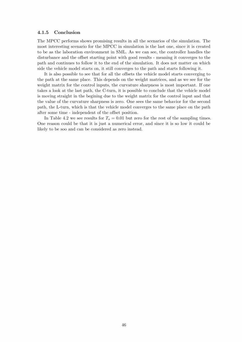
4.2.1 Path 1 - Straight Line

The implementation results of the straight line path with dense kink-points are presentedin the Fig. 4.13, and the numerical values are in Tab. 4.14.

Offset [m] 0.296Pos

RMSE

[m] 0.100Pos

MAX

[m] 0.075Trun

[s] 0.018

OffsetScaled [m] 9.457PosScaled

RMSE

[m] 3.202PosScaled

MAX

[m] 2.410

Table 4.14

�1.5 �1 �0.5 0 0.5 1 1.5 2 2.5

�0.2

�0.1

0

0.1

x [m]

y[m

]

Map

Refeerence Path, Simulation, Implementation, Kink-points.

0 0.5 1 1.5 2 2.5 3 3.5 4 4.50

0.1

0.2

0.3

0.4

Distance Traveled [m]

PositionError

[m]

Deviation from Path

Figure 4.13

47

4.2.2 Path 2 - Low Curvature Path

The implementation results of the low curvature path are presented in the Fig. 4.14, andthe numerical values are in Tab. 4.15.

Offset [m] 0.306Pos

RMSE

[m] 0.117Pos

MAX

[m] 0.078Trun

[s] 0.023


RMSE

[m] 3.747PosScaled

MAX

[m] 2.496

Table 4.15

�1.5 �1 �0.5 0 0.5 1 1.5 2 2.5 3

0

2

x [m]

y[m

]

Map


0 1 2 3 4 5 6 70

0.1

0.2

0.3

0.4


PositionError

[m]

Deviation from Path

Figure 4.14

48

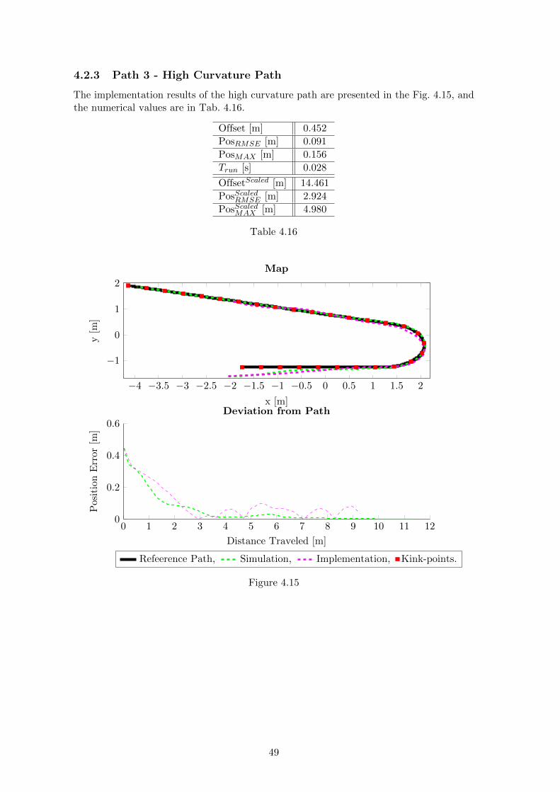
4.2.3 Path 3 - High Curvature Path

The implementation results of the high curvature path are presented in the Fig. 4.15, andthe numerical values are in Tab. 4.16.

Offset [m] 0.452Pos

RMSE

[m] 0.091Pos

MAX

[m] 0.156Trun

[s] 0.028


RMSE

[m] 2.924PosScaled

MAX

[m] 4.980

Table 4.16

�4 �3.5 �3 �2.5 �2 �1.5 �1 �0.5 0 0.5 1 1.5 2

�1

0

1

2

x [m]

y[m

]

Map


0 1 2 3 4 5 6 7 8 9 10 11 120

0.2

0.4

0.6


PositionError

[m]

Deviation from Path

Figure 4.15

49

4.2.4 Conclusion

The MPCC shows similar results as in the simulations, which is expected. The implemen-tation of the controller on the scaled-trucks shows that it converges to the path, but withdifficulties which is seen as the path of the vehicle has small bumps as it gets close to thereference path.

The tuning of the weight matrices for the system states and inputs varies from theones in simulation. The areason is that when the simulation weight matrices was used inthe implementation the controller did not find any feasible solutions and therefore it couldnot control the vehicle. The new set of weight matrices made the vehicle follow the path,but tuning these parameters could improve the path following.

If one look at the figure of the results, one can see tendensies to tiny oscillation behaviorof the vehicle. This could be from the fact that the mini-truck that is used is a toy modelof a real truck and therefore the performance of the mini-trucks are not perfect. Thismeans that the controller finds a reference the mini-truck should follow, but it cannotbecause of its limits in the actuators, sensors and motors.

50

Chapter 5

Conclusions and Discussions

The thesis describes an implementation of the Clothoid-based Model Predictive Control(MPCC) in the Smart Mobility Lab. We evaluate the performance of the controller insimulations and by experiments with 1:32 scaled radio trucks.

5.1 Conclusions

The implementation of the MPCC controller in SML shows promising results, since itmakes the vehicle converge to all the path when it starts with an offset, even if it has someproblems of remaining close to the path in implementation. The maximum deviation whenthe controller is implemented is 13.4cm for the high curvature path, and it is possible to seethat it is after the turn, the controller struggles to converge to the path. The computationtime for the MPCC algorithm is between 20 � 30ms, and the optimization problem inthe formulation of the MPCC is solved in less than 1ms. This could be due to that theimplementation of the MPCC algorithm is not optimized. Therefore, the efficiency of thealgorithm could be improved, but it shows that it is possible to implement the MPCC inSML for path following problem.

The MPCC controller shows that the need of a big horizon, i.e. a higher number ofpoints in the horizon, is not necessary needed when one uses space dependent modelsinstead of time dependent. It is clear that the QP solver is faster since the predictionhorizon is smaller, but the prediction of the behaviour of the model is calculated a fardistance ahead on the reference path.

The Smart Mobility Lab is a great platform for implementing novel ideas and controllersfor evaluation, but there exists limitations in the chosen equipment. The sensors are stateof the art, but the scaled-trucks are not. It is a simple toy, and has limitations. Theproblem is that it is not possible to get a better 1:32 scaled radio truck with better actuatorsor performance. The benefit is that the scaled-truck is sufficient good for an early phasein the development of a controller, so that it is possible to decide if the controller shouldbe implemented for more advanced systems, bigger vehicles, or even different vehicles. Anext step for the implementation of the controller could be the KTH Research ConceptVehicle (RCV), or even a heavy-duty vehicle. The RCV is filled with sensors, and performstests with different MPC approaches. It also introduces the possibility to investigate theperformance of the MPCC controller with a higher order model of the vehicle and findinga relation between the controller and the vehicle input.

51

Chapter 6

Future work

Continuing the development of the MPCC controller one could embody the velocity ofthe vehicle as an input variable for the controller. In this way, one could get a moreadjustable controller that could steer the vehicle better. An alternative step of this couldbe to implement a separable velocity controller and let the MPCC do the path followingfor the vehicle.

Before evolving the controller to handle the vehicle’s velocity, it could be trying toevade obstacles in the path. A challenge here would be to build clothoids around an object,and still be able to control the vehicle. An interesting approach would be to apply theclothoids to an existing on-line path planner that can already detect and avoid obstacle.Another approach could be that if the controller detects an obstacle, another controller isselected for the avoidance of the obstacle.

Another next step for the MPCC is to use it for HDV platooning or a real size ordinarycar. One example could be the RCV-car that is being used for another project in the samebuilding as the Smart Mobility Laboratory.

Another application could be to use it for path following with a quadrocopter. It ispossible to create 3D clothoids, and therefore one could develop an MPCC based on 3Dclothoids and investigate the possibilities of using the same technique as MPCC but forflying robots. This could be implemented and tested in SML because of the feedbacksystem and the quickness of the MPCC to solve a QP problem. Another approach couldbe to use the MPCC with 2D clothoids to control the quadrocopter in a 2D plane. Thiscould be achieved by using a controller that keeps the quadrocopter at a steady heightlevel, while it is moving with constant speed. One could possibly make the quadrocopterturn with a piecewise function.

The time consuming problem of finding good weight matrices could maybe be improvedby applying an evolutionary algorithm for tuning the weight matrices, or any machinelearning algorithm. This could be broaden to even more controllers such as a PID-controller.

52

Bibliography

[1] P. F. Lima, M. Trincavelli, J. Martensson, and B. Wahlberg, ‘‘Clothoid-based modelpredictive control for autonomous driving,’’ in European Control Conference (ECC),Linz, Austria, 2015.

[2] F. Borrelli, A. Bemporad, and M. Morari, Predictive Control for linear and hybridsystems, UC-Berkeley, 2015.

[3] P. Falcone, M. Tufo, F. Borrelli, J. Asgari, and H. Tsengz, ‘‘A linear time varyingmodel predictive control approach to the integrated vehicle dynamics control problemin autonomous systems,’’ in Decision and Control, 2007 46th IEEE Conference on.IEEE, 2007, pp. 2980--2985.

[4] F. Kuhne, W. F. Lages, and J. Gomes da Silva, ‘‘Mobile robot trajectory trackingusing model predictive control,’’ in II IEEE latin-american robotics symposium, 2005.

[5] R. Oliveira, ‘‘Planning and motion control in autonomous heavy-duty vehicles,’’Master’s thesis, KTH Royal Institute of Technology, 2014.

[6] P. F. Lima, ‘‘Implementation and analysis of platoon catch-up scenarios for heavyduty vehicles,’’ Master’s thesis, KTH Royal Institute of Technology, 2013.

[7] R. Rajamani, Vehicle dynamics and control. Springer Science & Business Media,2011.

[8] A. L. Cauchy, Lecons sur Les Applications du Calcul Infinitesimal a la Geometrie,1826, vol. 1.

[9] R. Oliveira, ‘‘Smart mobility lab mini trucks report,’’ KTH Royal Institute of Tech-nology, Tech. Rep., 2014.

[10] A. De Luca, G. Oriolo, and C. Samson, ‘‘Feedback control of a nonholonomic car-likerobot,’’ in Robot motion planning and control. Springer, 1998, pp. 171--253.

[11] S. Boyd and L. Vandenberghe, Convex optimization. Cambridge university press,2004.

[12] M. Morari and J. H. Lee, ‘‘Model predictive control: past, present and future,’’Computers & Chemical Engineering, vol. 23, no. 4, pp. 667--682, 1999.

[13] J. Mattingley and S. Boyd, ‘‘Cvxgen: a code generator for embedded convex optimiza-tion,’’ Optimization and Engineering, vol. 13, no. 1, pp. 1--27, 2012.

53

TRITA EE 2015:78ISSN 1653-5146

www.kth.se

implementation and analysis of a clothoid-based model...

Documents