IMPLEMENTATION OF REAL TIME GEOTECHNICAL MONITORING AT AN OPEN PIT MOUNTAIN COAL MINE IN WESTERN CANADA Brian Klappstein, M.Sc., PGeo., Manager of Long Range Planning, Grande Cache Coal LP, AB, Canada Gheorghe Bonci, PhD, PEng., Faculty at British Columbia Institute of Technology, BC, Canada Wayne Maston, PEng., Production Engineer Surface, Grande Cache Coal LP, AB, Canada ABSTRACT: The evolution of geotechnical monitoring technology for assessing slope stability issues in real time has progressed rapidly in the last few decades. The technology has advanced the safety of open pit operations and has the potential to change planning parameters, particularly in activities adjacent to public infrastructure, based on the additional confidence that operators gain from instantaneous access to information as pits are excavated and waste dumps are constructed. This paper summarizes the experience of a coal mine operating in the rugged topography of the Alberta foothills, excavating extremely structurally complex coal deposits within thrust and fold belt geology. In the last decade, the geotechnical monitoring at this site progressed from manual (daily to monthly) monitoring of a network of survey prisms and piezometer installations, to real time (hourly or less) monitoring of slopes and slope foundations by multiple robotic total stations sampling prism networks on pit walls and dumps, slope scanning radar, piezometers and some manually monitored borehole slope inclinometers. During this period, the mine experienced a number of slope failures on both pit walls and waste rock dumps. Back analysis of these failures from the monitoring data has refined the understanding of the speed failures progress at, and the best metrics and thresholds to define how alarm systems should respond to deformation. Case studies are presented for both pit foot wall and dump failures. KEYWORDS: Geotechnical, monitoring, back analysis, SSR, StdE

1. INTRODUCTION. GENERAL CONSIDERATIONS

The failure of slopes, both excavated pit wall slopes and waste rock dump slopes, is a significant safety issue in open pit mining. The challenge to find the balance between safety and economics starts with the process of geotechnical analysis of proposed open pit mine walls and dumps. However, even the most carefully researched and engineered designs are based on relatively simple models of a geologic environment which can never fully predict the variability of material structure and strength that exist in the real world. Simply put, practical limitations force the geotechnical engineer to make assumptions about the rock mass characteristics.

These assumptions, along with the imperfect translation by mine operations of the design into the as-mined geometry, introduce uncertainty and therefore the potential for failure of the excavation or the excavated material. The potential for failure is addressed by monitoring the excavation in progress for warning signs of impending catastrophic slope failure. There may or may not be an opportunity to stop an impending failure from happening, but personnel and equipment can be spared the

consequences with enough warning. The evolution of ever more complex geotechnical monitoring systems is driven by the desire to provide the earliest possible warning of impending slope failure.

The development of sophisticated monitoring systems is not only driven by the desire to simultaneously improve safety and mining economics, but also to meet the moral and legal obligations of mine owners to protect the workforce from harm. Government regulations may not specify the technical details of geotechnical monitoring systems, but the objective of legislation in protecting the workers by identifying, controlling and minimizing risk are clearly stated in Canadian regulations. Just as clear is the evolution in provincial jurisdictions across Canada over the last few decades in explicitly defining accountability and therefore liability for the safety of the worker from the very bottom to the very top of the chain of command. In these conditions a monitoring system for the open pit mine walls and waste dumps becomes a necessary and valuable tool for identifying potential slope failures before

250

the unstable rock mass becomes hazardous for personnel and equipment.

The objectives of a geotechnical monitoring system are:

• to protect personnel and equipment from the consequences of catastrophic slope failure by providing sufficient warning of an impending event;

• to provide enough time before a catastrophic slope failure event to allow action to prevent or mitigate the event;

• to assess the performance of pit and waste dump slope design and provide feedback on the assumptions and methods used to generate the design;

• to maximize the economics of the excavation, by limiting designs based on the confidence that a monitoring system can maintain a safe working environment, and

• to provide the level of data density in both the temporal and spatial senses that enables the continuous evolution of the monitoring system warning levels from back analysis of each instability event.

The scope of this paper is to consolidate, quantify where possible, and present experience gained in the evolution of geotechnical monitoring at a western Canadian open pit coal mine from manual methods to real time automated systems over the last 10 years. Discussion will center on the how implementing robotic total stations and slope stability radar for geotechnical monitoring enabled the early recognition of impending instability, and what was learned about interpreting the signs of impending slope failure by back analyzing a number of case studies.

2. SLOPE MONITORING SYSTEM AT GCC 2.1. Background 2.1.1. Geology, Terrain, Climate

This case study is based on an open pit coal mining

operation in the eastern foothills of the Rocky Mountains in west central Alberta, Canada. The operation mines Lower Cretaceous coal seams in a matrix of mostly non-marine sandstone siltstone and mudstone strata. The geologic structure is that of a thrust and fold belt, with the strata stacked by major thrust faulting and folded into chevron and box folds. The tectonic events which created these structures occurred 60 million years ago. Major fold axes typically have wavelengths between 200 and 1000 metres. Major thrust faults all verge northwest and are generally 2 to 6 kilometres apart measured across strike. Parasitic folding and smaller scale thrust faulting is pervasive on the limbs of the major folds (Langenberg, Kalkreuth, & Wrightson, 1987).

The strata are generally well cemented and in-situ

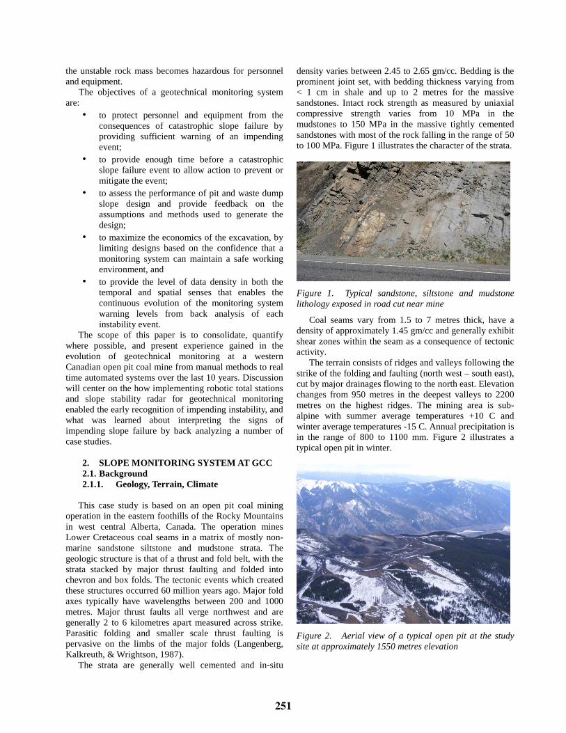
density varies between 2.45 to 2.65 gm/cc. Bedding is the prominent joint set, with bedding thickness varying from < 1 cm in shale and up to 2 metres for the massive sandstones. Intact rock strength as measured by uniaxial compressive strength varies from 10 MPa in the mudstones to 150 MPa in the massive tightly cemented sandstones with most of the rock falling in the range of 50 to 100 MPa. Figure 1 illustrates the character of the strata.

Figure 1. Typical sandstone, siltstone and mudstone lithology exposed in road cut near mine

Coal seams vary from 1.5 to 7 metres thick, have a density of approximately 1.45 gm/cc and generally exhibit shear zones within the seam as a consequence of tectonic activity.

The terrain consists of ridges and valleys following the strike of the folding and faulting (north west – south east), cut by major drainages flowing to the north east. Elevation changes from 950 metres in the deepest valleys to 2200 metres on the highest ridges. The mining area is sub-alpine with summer average temperatures +10 C and winter average temperatures -15 C. Annual precipitation is in the range of 800 to 1100 mm. Figure 2 illustrates a typical open pit in winter.

Figure 2. Aerial view of a typical open pit at the study site at approximately 1550 metres elevation

251

2.1.2. Mining History

Coal mining was initiated at the study site in 1969, and has been ongoing for 31 of the past 35 years, using both underground room and pillar and open pit truck and shovel operations. The surface operations began in 1972. The current operator has been mining on the property since 2004.

Open pit geometry is based on highwalls (pit slopes cutting across bedding joints) with overall angles between 45 and 53 degrees, and footwalls (pit slopes following bedding joints) with overall angles between 40 and 50 degrees. Pits walls are up to 200 metres high. Waste rock dumps are built both bottom up in lifts of 5 to 10 metres or dumped top down with crest to toe heights approaching 100 metres. Angle of repose for waste dumps is 36 to 37 degrees.

2.1.3. Geotechnical Monitoring History

The study property has a long history of geotechnical monitoring, using extensometers, prisms, and piezometers (Smoky River Coal Ltd, Piteau Associates Engineering Ltd, Alberta Office of Coal Research and Technology, 1987).

The current operator has continued with protocols adopted by the previous operator commencing in 2004 with manual monitoring methods. The primary tool used was a Geodimeter 444 total station (1” angle accuracy) mounted on steel casing cemented into bedrock with a mounting plate welded to the top. The station monitored corner cube electronic distance measurement (EDM) prisms mounted on steel rods, driven into the berms of waste dumps, or epoxied into holes drilled in the rock faces of the excavated pit walls. Prisms mounted on rock walls have small steel “hoods” above them to protect from debris falling down the wall. Experimentation with flat stick on EDM reflectors and clusters of reflectors showed this method could not obtain the required measurement accuracy for geotechnical monitoring of rock walls.

Depending on the proximity to operations and nature of the slope being monitored, monitoring frequency generally was daily and varied between 1 week and twice daily. This method was used until the first of four robotic total stations (Leica TM30, ½” angle accuracy) (Leica Geosystems AG, 2014) was installed in the fall of 2011. Locally-built weather protection shelters house the station mounted on steel casing cemented into a borehole as per previous practice (Figure 3). The power for these installations is provided by a combination of solar panels and small wind turbines. Communication is through a wireless network covering the mine site, using solar powered trailer mounted antennae (Tropos), which is also the communications for the equipment tracking and dispatch system.

Slope stability radar was first used on the property in the fall of 2010, initially with rentals deployed to monitor

slopes deemed to have borderline stability based on visual and EDM prism monitoring, and where retroactive installation of prisms was difficult. In the summer of 2012 the operator purchased a used GroundProbe SSR-X radar unit (GroundProbe Pty Ltd, 2014) which has been operating on demand since then. This unit has an effective range of approximately 3 km. Measurement resolution at the ranges typically used by the current operator is from 1 to 9 m vertically and horizontally (150 to 1000 metres range) with the reporting done using a vary-colored pixel map Figure 4 shows a typical monitoring scenario with the SSR-X unit.

Figure 3. Total station monitoring inside weather protection shelters house

Figure 4. SSR-X radar monitoring system

252

Figure 4 above shows a SSR-X radar monitoring system and figure 5 below shows a typical monitoring scenario with this unit.

Figure 5. SSR-X radar monitoring a pit footwall from an access ramp

In addition to the real time data available from the robotic total stations (RTS) and slope stability radar (SSR), the operator has installed a number of solar powered wireless connected vibrating wire piezometers (VWPs) to enable tracking groundwater levels in real time.

Specifically the installations are located in rock dumps above a public highway. Initially remotely monitoring of VWPs was done via satellite modems since wireless coverage of the study site had not been installed. Currently only the most critical VWPs are wired to be monitored in real time. Figure 6 shows a remotely monitored VWP installation.

Figure 6. Remotely monitored vibrating wire piezometer

2.2. Current Geotechnical Monitoring Methods

2.2.1. Guiding Principle

Slope failures do not occur spontaneously, and if an area is being well monitored the failure won’t occur without warning.

The first guiding principle of a monitoring system is to provide the resource of time, time to prevent, time to mitigate and above all time to evacuate personnel and equipment.

However, the warning provided by a geotechnical monitoring system is of no use unless it is communicated to the decision makers.

The second guiding principle is that the system must have a robust communications capability and protocol.

There is a scientific reason behind each slope failure, and understanding that science is the basis for improving a monitoring system.

The third guiding principle of a monitoring system is to provide the density and quality of data required for back analysis.

Geotechnical monitoring technology has evolved rapidly over the last generation (like all forms of technology). This additional complexity is a challenge as those with the skills to operate, maintain, and interpret the output of a monitoring system are hard to attract to the remote lifestyle of mining.

The fourth principle is simplicity; the system must be as simple as possible to operate and maintain, so those functions can be delegated to as wide a range of personnel as possible.

Considering the large areal extent of many open pit mines, each work site must have its own monitoring program and strategy based on local ground conditions. Hence the cost effectiveness and mobility of geotechnical monitoring elements is the fifth guiding principle of a monitoring system.

The monitoring methods used to observe the slope behaviour at the GCC mine site are a combination of surface and subsurface ones.

2.2.2. Implementation

The slope movement monitoring system at GCC was designed and is operated and maintained by a combination of in-house and contractor personnel. The implementation of the system had the full support of the operator’s senior management thus the evolution to the most advanced monitoring equipment was rapid. The geotechnical monitoring system is the responsibility of the Technical Service’s department at the study site.

The geotechnical monitoring system at the study site consists of both quantitative and qualitative elements. The qualitative assessments of the working conditions (including visual inspection to detect the onset of slope instability) are done by pit superintendent and pit supervisors and are required by the regulating bodies (in

253

this case the Occupation Health and Safety Act of Alberta).

The results of these visual observations made during the routine inspection are recorded in an inspection log. While these observations are subjective, they can prove invaluable in building up a history of rock mass behaviour for assessment of the pit slope conditions.

Quantitative elements of the geotechnical monitoring system are the subject of this paper. They involve a range of displacement monitoring equipment and techniques used to assess the ongoing stability of pit and waste dump slopes, and the subsidence over active underground mines.

They include: • survey monitoring (robotic total stations, and

manual total station monitoring, aero photogrammetric and airborne Lidar - light detection and ranging - surveys);

• displacement monitoring pins and wire extensometers, paint marking to detect offsets;

• borehole inclinometers; • vibrating wire piezometers (VWP), and • laser scanning (Slope Stability Radar unit – SSR)

The selection of monitoring methods used at the study site was designed to be the most cost effective based on the principles stated above and including the:

• accuracy level required; • robustness; • cost per method; • monitoring interval time (e.g. 24/7); • time taken to get the raw data; • time taken to process the acquired data; • access to the area of interest; • security of the system ; • existing trained personnel

The focus of this paper is the interpretation of failures using the primary real time components of the geotechnical monitoring system, the robotic total stations and slope stability radar.

2.2.3. Metrics

Slope failures in natural ground and open pit mines are always preceded by some amount of strain or deformation within slope; this is true for even the most brittle rocks and certainly true for jointed rock masses and unconsolidated sediments. Monitoring methods which seek to detect this deformation by measuring relative movement within a slope are direct monitoring methods. Indirect geotechnical monitoring methods measure parameters which affect a slope’s shear strength, such as groundwater pore pressure and temperature.

Direct monitoring methods include borehole inclinometers, wireline extensometers, EDM prisms, GPS antennae, and slope stability radar. All of these are discrete point systems with the exception of slope stability

radar. The effectiveness of the discrete point methods is dependent on the density of the monitoring points relative to the scale of impending slope failure the monitoring seeks to detect.

The different methods of slope monitoring capture multiple strain metrics, depending on the method. For example a borehole slope inclinometer captures shear magnitude and azimuth direction.

The focus of this paper, EDM prism surveying and slope stability radar capture movement.

In the case of the prism monitored by total station the movement is measured by changes in horizontal and vertical angle between the station and the prism and the distance between the station and the prism, known as slope distance.

Slope stability radar measures movement differently. The scanning radar beam reports changes in slope distance at fixed vertical and horizontal angles along the scan pattern. Hence changes in distance between the radar and reflections from a given azimuth, is the detection metric. The discrete increments in scan angle are called “pixels” and the metric is “delta range” for each pixel. Figure 7 shows the display of the radar scanning output and reference photographic montage captured by the radar unit.

Figure 7. Radar scanning pixel image, with associated reference photographic montage

The total station therefore tracks the three dimensional movement over time of a discrete point on the slope. However, while the 3D movement is the end result of the stations measurement system, the 3 inputs to that movement (horizontal and vertical angle, and slope distance) have differing levels of accuracy and this accuracy varies with distance.

To understand the real world accuracy in a mining environment, statistical analysis of the three outputs of vertical movement, horizontal movement and slope distance from a RTS monitoring prisms installed on waste rock dumps was analyzed. The analyzed scenario had prisms with ranges varying from 0.5 km to 1.1 km, and was done over a 1.5 month period where movement was apparent, but linear and predictable in nature.

254

The method was to choose a time interval over which any detectable deformation at a prism was linear, and perform regression analysis of the hourly data in that period, with the standard error of the regression interpreted as the noise component of the deformation measurement.

Then the noise statistic (StdE) for prisms at different distances from the monitor station was plotted. This analysis is shown in Figure 8. The assumption of linear deformation is not likely true in all cases, or perfectly true in any case, but the method is an initial attempt to understand the signal to noise relationship in deformation measurements.

Figure 8. Measurement error versus distance for vertical and horizontal angles, and slope distance from EDM prism monitoring, as measured by the standard error of linear regression of deformation traces over 1.5 months

As can be seen from Figure 8, the measurement variability increases with distance as expected, however the three outputs have different levels of variance.

The horizontal movement has the greatest error with distance. This is likely the result of errors in calibration of the horizontal angle using a fixed location back site prism. The vertical movement has slightly less variance error with distance.

The slope distance error is the most predictable of the three outputs.

Table 1. Regression Output Statistics, Standard Error versus Monitoring Distance

Trend mm/km

Intercept (mm)

Correlation

Coefficient Vertical Error vs Monitoring Distance 6.4 1.2 0.44 Horizontal Error vs Monitoring Distance 9.2 0.4 0.52 Slope Distance Error vs Monitoring Distance 4.6 0.7 0.85

All three outputs have error relationships with distance significantly above the specification of the RTS equipment, indicating that atmospheric conditions are the most significant contributor to measurement noise in the experience of the operator at the study site.

Statistics for the regression analysis in Figure 8 are presented in the above Table 1.

The noise in the radar output appears to be substantially less in the experience of the study mine operator. Noise was calculated by the same method as used for the RTS analysis.

Deformation data from a waste rock dump over time were analyzed by linear regression and the StdE of the regression was plotted and compared against other pixels at varying distances from the radar monitor. In this case the analysis period was 10 days, less than the RTS noise analysis period, but with a similar number of points as the radar acquires between 4 and 5 measurements per hour per pixel and the RTS (as used by this operator) captures only 1 measurement per hour.

The manual nature of extracting individual data points from the radar scanning databased limited the number of pixels analyzed. The results are shown in Figure 9 which also plots the slope distance metric error from the RTS noise analysis.

Radar noise appears very low in this example. The radar as used by this operator corrects for atmospheric conditions using a fixed known reflection area to calibrate the signal. The period analyzed did have significant variability in weather over the 10 day period (late October). Further investigation of different periods with more variability in the diurnal cycle will resolve the radar measurement noise in real world environments.

Figure 9. Measurement error versus distance, comparing prism monitoring slope distance metric to slope stability radar, as measured by the standard error of linear regression of deformation traces over time (period 1.5 months for prism monitoring and 10 days for radar monitoring)

2.2.4. Reporting Metrics

The threshold for generating a warning message from geotechnical monitoring systems is one of the most

255

critical decisions made by those charged with implementation. Thresholds set too low generate messages originating in either measurement noise or normal settlement or slope relaxation of waste rock dumps and pit walls respectively.

The framework for determining warning thresholds is complex for both SSR and RTS output. In the case of SSR, there is only one metric: delta range. However that metric has greatly differing magnitude relative to true 3D deformation depending on the angle between the radar beam and the slope being monitored. In the case of RTS, the output can be parsed into multiple useful metrics for a given prism movement being tracked over time: vertical movement, horizontal movement, 3D movement, slope distance, movement dip angle, and movement azimuth. These metrics can be presented as cumulative or instantaneous against time.

The choices for metrics to base warning thresholds on are varied but based on the experience at the study site, the most valuable metrics are those with the least noise, and those that allow inter-comparison between the two monitoring technologies.

In the case studies presented the objective is to back analyze failure and maximum deformations without failure and extract the thresholds for failure. To create a useful database for setting warning thresholds, it is desirable that metrics should be transferable from RTS to SSR and vice versa.

The radar monitoring only collects slope distance information. The RTS monitoring collects 3D movement which can be resolved into a number of metrics with different noise levels. In the order of least noise to most noise they are:

• slope distance velocity of discrete points; • vertical velocity of discrete points, and • 3D velocity of discrete points

Since 3D motion is the ultimately the metric that tells the most about slope failure, this was the metric chosen to present in the back analysis examples. Slope distance change measurements from the radar were converted to pseudo 3D movement using estimates of the failure vector azimuth and plunge. There is a large element of error potential in this method, but it is a first step in relating the radar “movement” to 3D deformation.

2.2.5. Water and Weather Metrics

In the climatic conditions, bedrock and foundation characteristics environment of the study property, groundwater changes have a clear involvement based on anecdotal experience. While not the focus of this paper, the example below clearly illustrates the relationship between ground water change and slope deformation. Figure 10 is a plot of time showing the settlement of a waste rock dump over 2.5 years monitored by a robotic total station, compared with the groundwater level as measured by piezometer.

Figure 10. Deformation rate of a waste rock dump 45 metres thick, compared to the groundwater level in the base of the dump, as measured by vibrating wire piezometer

The prism generating the data was approximately 10 metres away from a vibrating wire piezometer, which was also being monitored in real time. At this location the waste rock dump was less than 45 metres thick, the piezometer being located at the base of the dump at 48 metres depth. Waste rock dumps settle naturally over time but it is clear the settling rate accelerates when the water table rises.

Figure 11 shows the same time period but with the deformation in the dump converted to velocity using a rolling linear regression filter.

The clear relationship between the dump deformation rate and the water table in this example shows that a key metric for a total system is weather.

It is expensive to install piezometers above pit high walls, and all but impossible to install them in an active waste dump, but weather is a metric which is included in most real time EDM and radar monitoring systems since they use these metrics to correct for atmospheric conditions.

Figure 11. Deformation rate of a waste rock dump compared to groundwater level at the base of the dump as measured by vibrating wire piezometer

2.3. Results 2.3.1. Back Analysis Examples

The back analyses of failures and near failures on the

study site presented here are based on both manual and

256

automated real-time reporting geotechnical monitoring systems, both SSR and RTS based. Unfortunately, no failure was observed by SSR and RTS monitoring simultaneously.

However, converting slope distance velocity to 3D velocity using the angle between the failure vector and the scanning vector, is first step to creating a database that is useful in setting warning thresholds for both monitoring technologies.

• Case study 1: 12 South B2 NW Footwall

Failure

This failure occurred in June of 2006 at the study site on a pit footwall dipping approximately 52 degrees, when approximately 5,000 bank cubic metres of rock in a slab approximately 6 metres thick failed. It is unique in these examples in that the wall was supported by tensioned rock anchors 8 metres long on a spacing approximately 3.5 metres horizontal by 5 metres vertical. This failure has been analyzed and documented previously, although not using the metric of slope distance, the least noisy measurement parameter (KEH & Associates Ltd., 2006).

Monitoring was by EDM prisms, monitored manually on a daily basis. Figures 12 and 13 show before and after photographs of the slide. Interpolations of the velocity of 3D movement at the moment of failure by generating a best fit equation from selected measurement points using exponential regression. This equation was used to calculate the velocity at the instant of failure. The choice of measuring points is subjective and was guided by the correlation coefficients of the regression trials.

Figure 12. Pre-failure photograph, June 20, 2006 event, showing prism locations (after KEH 2006)

Figure 13. Post failure photograph of June 30, 2006 event, showing approximate original location of Prism 41

Figure 14 shows a graph of 3D movement over time and the exponential regression and velocity for a prism located in the approximate center of the failed block prior to the failure.

Figure 14. Manual daily monitoring measurements preceding June 30, 2006 failure and velocity estimate from exponential regression

The regression analysis of Prism 41 on the failed footwall block indicates 3D velocity at the instant of failure was 55 mm/day or 2.3 mm/hour. The scatter on the measurement points is large at this relatively low deformation rate and is a result of the lower resolution monitoring instrument.

• Case study 2: 8 North Footwall Failure

A pit footwall failure similar to the June 30, 2006 event occurred on May 5, 2014. This failure differed in that the monitoring was done with a RTS with better precision, monitoring on an hourly basis, as opposed to daily manual monitoring.

The failed block in this case was similar in size, rock quality, and failure plane dip along bedding. The differences were that the wall was not supported by tensioned rock anchors and the failed slab was thinner, being approximately 3.5 metres in thickness. Total failed

257

volume was approximately 2500 bank cubic metres. Figures 15 and 16 are photographs of the pre-failure and post-failure wall. Figure 17 shows a graph of 3D movement over time and the exponential regression and velocity for a prism located in the crest of the failed block prior to the failure.

Figure 15. Pre-failure photograph of May 5, 2014 event showing location of Prism 42N

Figure 16. Post failure photograph, May 5, 2014 event

Figure 17. RTS hourly measurement data preceding May 5, 2014 failure, and velocity from non-linear regression analysis

The anomalous nature of the last measurement data point made interpretation of the 3D velocity at failure difficult to interpret. Linear velocity over the last hour is extremely high, approximate 130 mm/hour. However, exponential regression of the last few hours of data,

excluding the final point, interpolates the velocity at failure to be much lower, 260 mm/day or 11 mm/hour. This example illustrates the challenge in back analysis of failure where any one data point is subject to the noise of back site errors, sudden weather changes etc. In the case of this example, analysis of surrounding prisms outside the unstable error indicates there were no shifts of the global prism population, meaning the final data point is valid within the measurement error at this range (+/- < 10 mm).

• Case study 3: Saddle Dump Failure

On the morning of July 27, 2011 at the study site, a waste rock dump slope failure occurred. The failure occurred via a liquefaction flow slide of the material underlying the dump toe. At the time of the event, the dump crest to toe height was approximately 100 metres. Figure 18 shows a photograph of the waste dump immediately post failure, with estimates of the pre-failure location of two monitoring prisms in the toe area of the failure.

There were no active prisms on the crest of the dump at the time of the event. Figures 19 and 20 show manual monitoring measurements of the prism movement in the days preceding the failure, and velocity estimates of the prism movement at the instant of failure from exponential regression.

Figure 18. Post failure photograph, July 27, 2011, showing the location of monitoring prisms 47 and 48

Figure 19. Prism 47 measurements preceding the July 27, 2011 failure and velocity estimate at failure from exponential regression

258

Figure 20. Prism 48 3D movement measurements preceding the July 27, 2011 failure and velocity estimate at failure from exponential regression

The prisms in the toe area of the dump were being monitored on a daily basis. The dump failure occurred early enough in the morning that the daily prism check was not done.

Velocity at the moment of failure was extrapolated using non-linear regression, but this shows the weakness of the historical monitoring methods compared to the real time systems currently in use. Velocity from both back analyzed prism movement shows 3D deformation was remarkably consistent between prisms (4800 to 4300 mm/day or 200 to 180 mm/hour).

• Case study 4: 8 South FW

A pit footwall failure on July 16, 2012 was captured by Slope Stability Radar. This was a relatively small scale failure having the dimensions in of 7 metres high by 8 metres wide by approximately 2 metres thick. Figure 21 is a photograph of the post-failure area. Figure 22 shows the monitoring data captured by the SSR unit.

Figure 21. Analysis area post failure, July 16, 2012

Resolution of the radar delta range metric into true 3D motion was done geometrically using these assumptions:

• the failure plane was dipping out of the wall at 60 degrees;

• the radar beam was horizontal to the monitored pixel;

• the radar beam was perpendicular to the strike of the failure plane, and

• the bright spot reflector within the pixel moved with the deforming failure block

Figure 22. Radar range measurement screen capture, July 16, 2012

As can be seen by the green square (monitored output pixel for this analysis) inside the red square in the photographic montage taken by the radar Figure 22, the geometry of the beam is close to horizontal to the target. Less easy to see, but verifiable in plan view is the perpendicular relationship of the radar beam and the pit wall strike. With the assumptions above the conversion from range to 3D motion is simple:

• delta range/cosine(60) = delta 3D movement

Plotting the 3D movement versus time and regressing movement versus time to obtain a smoothed velocity function over time is shown in Figure 23. The short sampling interval means this smoothing by regression process is not required as in previous analysis, but the analysis is useful in that it shows that deformation of rock slopes is an exponential process. Velocity at failure was 1010 mm/day or 42 mm/hour.

Figure 23. Radar range measurements converted into estimated 3D velocity, July 16, 2012

259

• Case study 5: 8 Middle Till Highwall

This study area did not experience a failure during the monitoring period. The problem which initiated the deployment of the SSR unit was a thick till layer hanging above a pit highwall which showed visual indications of instability.

The radar was deployed through the summer and early fall of 2013. This back analysis attempts to resolve the maximum 3D velocity of the till highwall cut face during the period when the pit bottom below the highwall was excavated.

Figure 24 shows the location of the unstable area on the highwall using the radar monitoring screen capture. Figure 25 is the analysis conducted on the radar range measurements over the 3 month period. The radar range was converted to 3D velocity using estimates of the main movement vector of the till along the bedrock interface, and the beam angle to the analysis zone from the radar unit. Using the dot product of the vectors the angle between movement and the radar beam vectors was resolved to be approximately 52 degrees. A rolling 1 day linear trend of the data (approximately 90 scans per day) was used to smooth the velocity. Maximum velocity was 320 mm/day or 15 mm/hour. This occurred after periods of rain culminating in a 2 hour 1” of rainfall event.

Figure 24. Radar monitoring, summer 2013, showing area of instability on till highwall above excavated pit

Figure 25. 3D velocity analysis, till highwall instability region, summer 2013

2.4. Conclusions

Comparison of the case study back analyses, and real world results of historical and current technologies employed at the study site shows the evolution of geotechnical monitoring has resulted in large improvements in the ability to detect and understand impending slope failure.

This improvement is the result of both better discernment of the deformation signal from the measurement noise, and the greater spatial and temporal coverage of the current technologies. This signal to noise issue is one of the key impediments to further improvements in the warning lead time for impending slope failure. Further improvement will come from more detailed analysis of the vast amounts of data gathered by this new technology.

Two elements of the monitoring system form the core of the advances in geotechnical monitoring at the study site: Robotic Total Stations and Slope Stability Radar. A comparison of the strengths and weaknesses of each system is appropriate.

2.4.1. Methods Comparison Slope Stability Radar versus Robotic Total Stations

The experience of the operator at the study site is

based on approximately three years of simultaneous use of these two technologies for geotechnical monitoring. In addition the current operator has 10 years of total station prism monitoring experience at this mine site.

This experience forms the valid basis for a comparison of the real world performance of the two complementary technologies.

While these conclusions may not necessarily be the experience of all operators due to local climate, terrain, economics, personnel skill levels and choice of vendor for each technology, the experience at the study site can be summed up in the following table:

Monitoring Technology

Advantages Comments

Robotic Total Station

Purchase Cost Approximately $CDN60K per installation

Tracks 3D deformation

Interpretation is of output is more straight forward; back analysis can be more sophisticated

Reliable Is enclosed in a heated an wind/precipitation protected shelter

260

Visual Referencing

The prism location is known exactly so the visual interpretation of the location of detected instability is unambiguous

Slope Stability Radar

Sensitivity Less noise in range metric than slope distance metric from RTS

Weather immunity

Fog, snow can be seen through, there is a limit however

Continuous coverage

Radar scanning gives continuous coverage

Mobility Can be moved in approximately 3 hours

Monitoring Technology

Disadvantages Comments

Robotic Total Station

Atmospheric Correction

Significant noise relative to the diurnal temperature cycle for slope distance, and other atmospheric variables

Weather Interruptions

Can’t see through fog, heavy rain and snow or high levels of dust

Discrete points only

Coverage is dependent on the installation of reflectors, which are only feasible to install during the excavation

Time to set up Units require weather protection, so installations are more complex, and time consuming to set up

Slope Stability Radar

Purchase Cost Approximately $CDN450K per

installation Range is the

only primary metric

Interpretation of the “towards and away” metric of radar is not as straight forward as motion resolved into 3D

Operating cost Requires a diesel generator running for power supply, is exposed to the weather, in this case -35C to +32C, and very high winds

Visual Referencing

The pixel image of movement on a monitored slope can be overlain by photo montage taken regularly by the SSR unit, however the calibration of view angle between the photos and the radar beam is imperfect, plus at longer ranges the pixels are up to 9 metres square so it is not always exactly clear where small scale events are occurring on the slope

Table 2. A comparison of the relative advantages and disadvantages between RTS and SSR

The comparison between RTS and SSR technology

would not be complete without some qualifiers based on the experience of the operator of this study site.

The SSR is expensive but mobile. Therefore one unit can cover whichever slope is deemed the most critical from the perspective signs of instability. The SSR can provide coverage of slopes where there are no prisms, either because the slope was not foreseen to have a high potential for instability, or manpower or safety reasons.

The lower cost per installation of the RTS enables multiple installations for slopes deemed to require real time monitoring. When a slope is monitored using both radar and prisms, the 3D movement deformation vectors from the prisms help interpret the delta range metric from the radar.

Summarizing the experience at the study site, these are complementary, not competing technologies.

261

2.4.2. Signal, Noise and Thresholds

Extracting the deformation velocity signal from the measurement noise is one of the most challenging aspects of setting warning alarm thresholds.

Experience gained at the study site with multiple back analyzed failures shows the evolution of the monitoring system from manual methods to 24/7 real time automated systems have improved the ability to understand the real deformation rate from the noise.

The 20 to 30 fold increase in temporal data density has shown that weather is a major cause of noise in the measurement data. The real world magnitude of these errors could not have been quantified without the implementation of robotic total station systems.

Back analysis from case study examples shows a wide range of 3D velocities are apparent on rock slope walls. The range for rock slopes failure threshold 3D velocity is between 2.3 mm/hour and 130 mm/hour in the cast studies presented.

This wide range is partially the result of comparing supported to non-supported slopes, comparing crest area velocities to toe area velocities, comparing different technologies and comparing very different sampling rates.

Only one case study for waste rock dump failures was available and this failure was not well documented having only manual monitoring and an absence of prisms at the dump crest. Failure velocities in the foreground area of the toe reached between 180 and 198 mm/hour immediately prior to the failure event.

Data available from the real time geotechnical monitoring database shows that dump crests can move as fast as 25 mm/hour downward without failure occurring. Data on dump settlement rates shows that these can increase by a factor of 5 during heavy precipitation periods (from 0.02 mm/hour to 0.5 mm/hour).

2.4.3. Future Enhancements

Analyses presented in this paper are only the first step in improving the capability of a geotechnical monitoring system.

To date, the analysis of the output of the current real time geotechnical monitoring system has focused on understanding the noise component of the RTS measurements, and back analyzing 3D velocity change and the velocity threshold for rock slope failure. Further refinement of the monitoring sensitivity may come from analysis of these elements:

• the resolution of 3D motion vectors over time and by failure zone (crest, middle and toe);

• processing algorithms to reduce weather induced noise;

• the impact of weather on slope deformation rates, • the relationship between groundwater level and

precipitation rates; • the resolution of SSR range and RTS slope

distance using simultaneously gathered data, and • the relationship between the low noise metrics of

RTS slope distance and SSR range with true 3D motion.

3. ACKNOWLEDGEMENTS

The authors of this paper would like to thank Grande Cache Coal for access to their geotechnical monitoring database and Technical Services personnel with knowledge of the history and specifications of the geotechnical monitoring system. The authors would also like to thank GroundProbe Pty Ltd. for assistance in the preparation of this paper. 4. LITERATURE REFERENCES GroundProbe Pty Ltd. Slope Stability Radar Brochure.

Retrieved August 29, 2014, from http://www.groundprobe.com/CMS/Uploads/file/ProductFlyer_SSR_A4_web.pdf (2014).

KEH & Associates Ltd. 12SB2 Pit – Bolted Footwall Slide Investigation. Sherwood Park, AB: Commissioned internal report (2006).

Langenberg, C., Kalkreuth, W., & Wrightson, C. Deformed Lower Cretaceous coal-bearing strata of the Grande Cache area, Alberta. Edmonton, AB: Alberta Geological Survey (1987).

Leica Geosystems AG. Leica TM30. Retrieved August 29, 2014, from http://www.leica-geosystems.com/en/Leica-TM30_77983.htm (2014).

Smoky River Coal Ltd, Piteau Associates Engineering Ltd, Alberta Office of Coal Research and Technology. Final Report on Upper East Limb Open Pit Rock Anchoring and Slope Monitoring Project. Edmonton, AB: Office of Coal Research and Technology (1987).

262