in the name of allah decision making by using the theory of evidence students: hossein shirzadeh,...

1

IN THE NAME OF ALLAH

DECISION MAKING BY USINGTHE THEORY OF EVIDENCE

STUDENTS:HOSSEIN SHIRZADEH, AHAD OLLAH EZZATI

SUPERVISOR:Prof. BAGERI SHOURAKI

SPRING 2009

2

OUTLINES

INTRODUTION

BELIEF

FRAMES OF DISCERNMENT

COMBINIG THE EVIDENCE

ADVANTAGES OF DS THEORY

DISADVANTAGES OF DS THEORY

BASIC PROBABLITY ASSIGNMENT

BELIEF FUNCTIONS

DEMPSTER RULE OF COMBINATION

ZADEH’S OBJECTION TO DS THEORY

GENERALIZED DS THEORY

AN APPLICATION OF DECISION MAKING METHOD

3

INTRODUCTION

Introduced by Glenn Shafer in 1976“A mathematical theory of evidence”

A new approach to the representation of uncertainty

What means uncertainty? Most people don’t like uncertainty

ApplicationsExpert systemsDecision makingImage processing, project planning,

risk analysis,…

4

INTRODUCTION

All students of partial belief have tied it to Bayesian theory and

I. Committed to the value of idea and

defend it

II. Rejected the theory (Proof of

inviability)

5

• : Finite set• Set of all subsets :•

• Then Bell is called belief function on

INTRODUCTIONBELIEF FUNCTION

2]1,0[2: Bel

)...()1(...)()(

)...()3(

1)()2(

0)()1(

11

1

nn

jijii

i

n

BelBelBel

Bel

Bel

Bel

6

INTRODUCTIONBELIEF FUNCTION

is called simple support function if

There exists a non-empty subset A of and that

]1,0[2: Bel

0 1s

0

( )

1

if B does not contain A

Bell B s if B contain A but B

if B

7

INTRODUCTIONTHE IDEA OF CHANCE

For several centuries the idea of numerical degree of belief has been identified with the idea of chance.

Evidence Theory is intelligible only if we reject this unification

Chance : A random experiment : unknown outcome The proportion of the time that a particular one

the possible outcomes tends to occur

8


]1,0[: q

1)( x

xq

• Chance density– Set of all possible outcomes :X– Chance q(x) specified for each possible

outcome

– A chance density must satisfy :

9

• Chance function– Proportion of time that the actual

outcome tends to be in a particular subset of X.

– Ch is a chance function if and only it obeys the following


Ux

xqUCh )()(

)()()(

,)3(

1)()2(

0)()1(

VChUChVUChthen

VUandVUif

Ch

Ch

10

INTRODUCTIONCHANCES AS DEGREES OF BELIEF

• If we know the chances then we will surely adopt them as our degrees of belief

• We usually don’t know the chances– We have little idea about what

chance density governs a random experiment

– Scientist is interested in a random experiment precisely because it might be governed by any one of several chance densities

11

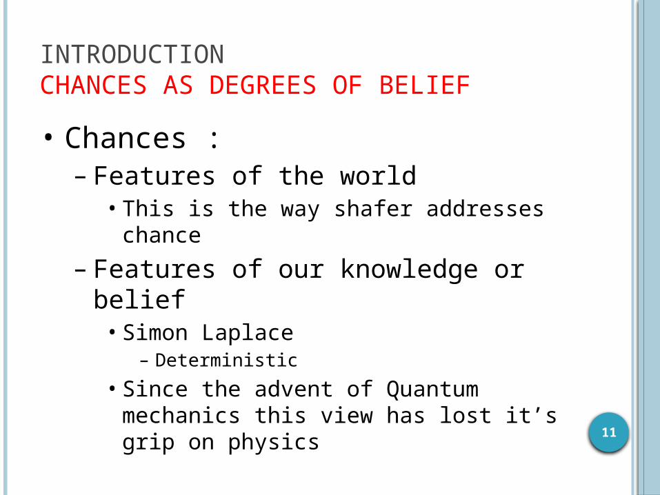
INTRODUCTIONCHANCES AS DEGREES OF BELIEF

• Chances : – Features of the world

• This is the way shafer addresses chance

– Features of our knowledge or belief• Simon Laplace

– Deterministic

• Since the advent of Quantum mechanics this view has lost it’s grip on physics

12

INTRODUCTIONBAYESIAN THEORY OF PARTIAL BELIEF

• Very Popular theory of partial belief– Called Bayesian after Thomas Bayes

• Adapts the three basic rules for chances as rules for one’s degrees of belief based on a given body of evidence.

• Conditioning : changing one’s degree of belief when that evidence is augmented by the knowledge of a particular proposition

13


(1) ( ) 0

(2) ( ) 1

(3) , ) ( ) ( )

Bel

Bell

If A B then Bell A B Bell A Bell B

:2 [0, 1]Bell obey s

When we learn that is true thenA

( )(4) ( )

( )A

Bell A BBell B

Bell A

14


• The Bayesian theory is contained in Shafer’s evidence theory as a restrictive special case.

• Why is Bayesian Theory too restrictive?– The representation of Ignorance– Combining vs. Conditioning

15


THE REPRESENTATION OF IGNORANCEIn Evidence Theory• Belief functions

– Little evidence:• Both the proposition and it’s

negation have very low degrees of belief

– Vacuous belief function

Aif

AifABel

1

0)(

16

INTRODUCTIONBAYESIAN THEORY OF PARTIAL BELIEFCOMBINATION VS. CONDITIONING

• Dempster rule– A method for changing prior opinion in

the light of new evidence• Deals symmetrically with the new

and old evidence

• Bayesian Theory– Bayes rule of conditioning

• No Obvious symmetry • Must assume exact and full effect of

the new evidence is to establish a single proposition with certainty

17

• In Bayesian Theory:– Can not distinguish between lack of belief and

disbelief– can not be low unless is high– Failure to believe A necessitates accordance of belief

to

– Ignorance represented by :

– Important factor in the decline of Bayesian ideas in the nineteenth century

– In DS theory

INTRODUCTIONBAYESIAN THEORY OF PARTIAL BELIEFTHE REPRESENTATION OF IGNORANCE

)(ABel

( )Bel AA

1( ) ( )

2Bel A Bel A

1 A)Bel(Bel(A)

BELIEF

The belief in a particular hypothesis is denoted by a number between 0 and 1

The belief number indicates the degree to which the evidence supports the hypothesis

Evidence against a particular hypothesis is considered to be evidence for its negation (i.e., if Θ = {θ1, θ2, θ3}, evidence against

{θ1} is considered to be evidence for {θ2,

θ3}, and belief will be allotted accordingly)18


Dempster - Shafer theory assumes a fixed, exhaustive set of mutually exclusive events

Θ = {θ1, θ2, ..., θn}

Same assumption as probability theory

Dempster - Shafer theory is concerned with the set of all subsets of Θ, known as the Frame of Discernment

2Θ = {f, {θ1}, …, {θn}, {θ1, θ2}, …, {θ1, θ2, ... θn}}

Universe of mutually exclusive hypothesis

19


A subset {θ1, θ2, θ3} implicitly

represents the proposition that one of θ1, θ2 or θn is the case

The complete set Θ represents the proposition that one of the exhaustive set of events is true

So Θ is always true

The empty set represents the proposition that none of the exhaustive set of events is true

So always false

20

21

COMBINING THE EVIDENCE

Dempster-Shafer Theory as a theory of evidence has to account for the combination of different sources of evidence

Dempster & Shafer’s Rule of Combination is a essential step in providing such a theory

This rule is an intuitive axiom that can best be seen as a heuristic rule rather than a well-grounded axiom.

22

ADVANTAGES OF DS THEORY

The difficult problem of specifying priors can be avoided

In addition to uncertainty, also ignorance can be expressed

It is straightforward to express pieces of evidence with different levels of abstraction

Dempster’s combination rule can be used to combine pieces of evidence

23

DISADVANTAGES

Potential computational complexity problems

It lacks a well-established decision theory whereas Bayesian decision theory maximizing expected utility is almost universally accepted.

Experimental comparisons between DS theory and probability theory seldom done and rather difficult to do; no clear advantage of DS theory shown.

24

BASIC PROBABILITY ASSIGNMENT

The basic probability assignment (BPA), represented as m, assigns a belief number [0,1] to every member of 2Θ such that the numbers sum to 1

m(A) represents the maesure of the belief that is committed exactly to A (to individual element A and to no smaller subset)

A

Am

m

1)()2(

0)()1(

25

BASIC PROBABILITY ASSIGNMENTEXAMPLE

suppose Diagnostic problem

No information

60 of 100 are blue

30 of 100 are blue and rest of them are black or yellow

1)( m

4.0)(

6.0})({

m

Bluem

0)(

7.0}),({

3.0})({

m

YellowBlackm

Bluem

},,,{ OtherYellowBlackBlue

25

26

BELIEF FUNCTIONS

Obtaining the measure of the total belief committed to A:

Belief functions can be characterized without reference to basic probability assignments:

AB

BmABel )()(

InI Ii

iI

n BelBel

Bel

Bel

,...,1

11 )(1)...(.3

1)(.2

0)(.1

27

BELIEF FUNCTIONS

For Θ = {A,B}

BPA is unique and can recovered from the belief function

BABelBBelABelBABel )()()(

BBelAmAB

BA

)1()(

28

BELIEF FUNCTIONS

Focal element A subset is a focal element if m(A)>0

Core The union of all the focal elements.

Theorem

BCoreBBelB 1)(,

29

BELIEF FUNCTIONSBELIEF INTERVALS

Ignorance in DS Theory:

The width of the belief interval:

The sum of the belief committed to elements that intersect A, but are not subsets of A

The width of the interval therefore represents the amount of uncertainty in A, given the evidence

1 A)Bel(Bel(A)

A)]- Bel([Bel(A), 1

30

One’s belief about a proposition A are not fully described by one’s degree of belief Bel(A) Bel(A) does not reveal to what extend one doubts A

Degree of Doubt:

Upper probability:

The total probability mass that can move into A.

BELIEF FUNCTIONSDEGREES OF DOUBT AND UPPER PROBABILITIES

)()( cABelADou

)(1)(* ADouAP

ABABB

c BmBmBmABelAPc

)()()()(1)(*

30

31

BELIEF FUNCTIONSDEGREES OF DOUBT AND UPPER PROBABILITIESEXAMPLE

Subset m Bel Dou P*

{} 0 0 1 0

{1} 0.1 0.1 0.5 0.5

{2} 0.2 0.2 0.4 0.6

{3} 0.1 0.1 0.4 0.6

{1, 2} 0.1 0.4 0.1 0.9

{1, 3} 0.2 0.4 0.2 0.8

{2, 3} 0.2 0.5 0.1 0.9

{1, 2, 3} 0.1 1 0 1

m({1, 2}) = – Bel({1}) – Bel({2}) + Bel({1, 2}) = – 0.1 – 0.2 + 0.4

32

BELIEF FUNCTIONS BAYESIAN BELIEF FUNCTIONS

A belief function Bel is called Bayesian if Bel is a probability function.

The following conditions are equivalent

Bel is Bayesian

All the focal elements of Bel are singletons

For every A⊆Θ,

The inner measure can be characterized by the condition that the focal elements are pairwise disjoint.

1 A)Bel(Bel(A)

33

BELIEF FUNCTIONS BAYESIAN BELIEF FUNCTIONSEXAMPLE Suppose },,{ cba

Subset BPA Belief

Φ 0 0

{a} m1 m1

{b} m2 m2

{c} m3 m3

{a, b} 0 m1 + m2

{a, c} 0 m1 + m3

{b, c} 0 m2 + m3

{a, b, c} 0 m1 + m2 + m3 = 1

34

DEMPSTER RULE OF COMBINATION

Belief functions adapted to the representation of evidence because they admit a genuine rule of combination.

Several belief functions

Based on distinct bodies of evidence

Computing their “Orthogonal sum” using Dempster’s rule

35

DEMPSTER RULE OF COMBINATIONCOMBINING TWO BELIEF FUNCTIONS

m1: basic probability assignment for Bel1 A1,A2,…Ak : Bel1’s focal elements

m2: basic probability assignment for Bel2 B1,B2,…Bl : Bel2’s focal elements

36


Probability mass measure of m1(Ai)m2(Bj) committed to

ji BA

37


The intersection of two strips m1(Ai) and

m2(BJ) has measure m1(Ai)m2(BJ) , since it is

committed to both Ai and to BJ , we say that the

joint effect of Bel1 and Bel2 is to commit exactly

to

The total probability mass exactly committed to A:

ji BA

)()(,

21 ABA

jiji

ji

BmAm

38

DEMPSTER RULE OF COMBINATIONCOMBINING TWO BELIEF FUNCTIONSEXAMPLE

m1({1}) = 0.3 m1({2}) = 0.3 m1({1, 2}) = 0.4

m2({1}) = 0.2 {1}, 0.06 Φ, 0.06 {1}, 0.08

m2({2}) = 0.3 Φ, 0.09 {2}, 0.09 {2}, 0.12

m2({1, 2}) = 0.5

{1}, 0.15 {2}, 0.15 {1,2}, 0.2

Subset Φ {1} {2} {1, 2}

mc 0.15 0.29 0.36 0.2

39

DEMPSTER RULE OF COMBINATION COMBINING TWO BELIEF FUNCTIONS

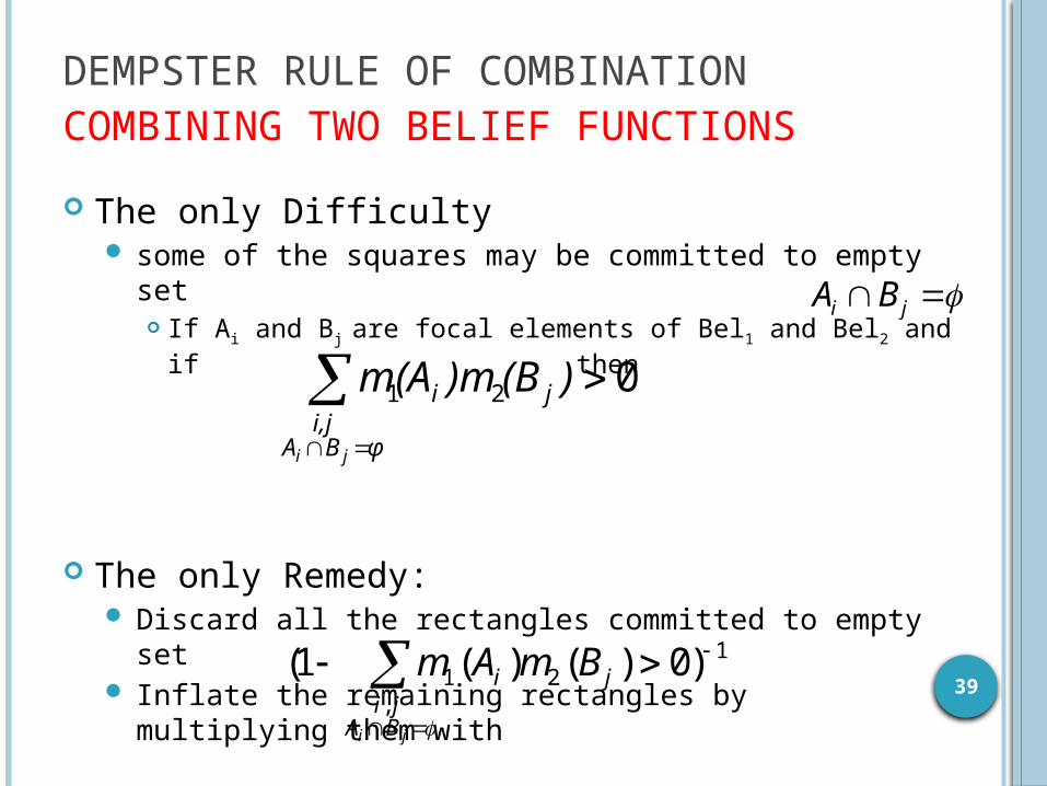
The only Difficulty some of the squares may be committed to empty set

If Ai and Bj are focal elements of Bel1 and Bel2 and if then

The only Remedy: Discard all the rectangles committed to empty set Inflate the remaining rectangles by multiplying them

with

ji BA

021

)(B)m(Am

φBAi,j

ji

ji

1

,21 )0)()(1(

ji BA

jiji BmAm

40

DEMPSTER RULE OF COMBINATION THE WEIGHT OF CONFLICT

The renormalizing factor measures the extent of conflict between two belief functions.

Every instance in which a rectangle is committed to corresponds to an instance which Bel1 and Bel2 commit probability to disjoint subsets Ai and Bj

k)()k

((K)

kK

)(B)m(Amk

φBAi,j

ji

ji

1log1

1loglog

1

1

21

41

DEMPSTER RULE OF COMBINATION THE WEIGHT OF CONFLICT (CONT.)

Bel1 , Bel2 not conflict at all:

k = 0, Con(Bel1, Bel2)= 0

Bel1 , Bel2 flatly contradict each other:

does not exist

k = 1, Con(Bel1, Bel2) = ∞

In previous example k = 0.15

21 BelBel

42

DEMPSTER’S RULE OF COMBINATION

Suppose m1 and m2 are basic probability functions over Θ. Then m1⊕m2 is given by

In previous example

Subset Φ {1} {2} {1, 2}

m=m1⊕m

20 0.3412 0.4235 0.2353

43

DEMPSTER RULE OF COMBINATION AN APPLICATION OF DS THEORY

Frame of Discernment: A set of mutually exclusive alternatives:

All subsets of FoD form:

WALKSTANDSIT ,,

WALKSTANDSIT

WALKSTANDWALKSIT

STANDSITWALKSTANDSIT

,,

,,,,

,,,,,{},

2

44


Exercise deploys two “evidences in features” m1 and m2

m1 is based on MEAN features from Sensor1

m1 provides evidences for {SIT} and {¬SIT}

({¬SIT} = {STAND, WALK})

m2 is based on VARIANCE features from Sensor1

m2 provides evidences for {WALK} and {¬WALK }

({¬WALK } = {SIT, STAND})

45


AB

* BmABel(A)PPls(A)Pl(A) 11

46

DEMPSTER RULE OF COMBINATION AN APPLICATION OF DS THEORYCALCULATION OF EVIDENCE M1

z1=mean(S1)

Evidence

Concrete value z1(t)

Bel(SIT) = 0.2Pls(SIT) = 1 - Bel(¬SIT) = 0.5

m1Concrete Value(SIT, ¬SIT, ) = (0.2, 0.5, 0.3)

47

DEMPSTER RULE OF COMBINATION AN APPLICATION OF DS THEORYCALCULATION OF EVIDENCE M2

z2=variances(S1)Concretevalue z2(t)

Bel(WALK) = 0.4Pls(WALK) = 1-Bel(¬WALK) = 0.5

Evidence

m2Concrete Value(WALK, ¬WALK, ) = (0.4, 0.5, 0.1)

48

DEMPSTER RULE OF COMBINATION AN APPLICATION OF DS THEORYDS THEORY COMBINATION Applying Dempster´s Combination Rule:

Due to m({}) Normalization with 0.92 (=1-0.08)

21 mmm

m1(SIT) = 0.2m1(¬SIT) =

m1(STAND,WALK) = 0.5m1(ALL) = 0.3

m2(WALK) = 0.4 m({}) = 0.08 m(WALK) = 0.2 m(WALK) = 0.12

m2(¬WALK) = m2(STAND,SIT) = 0.5 m(SIT) = 0.1 m(STAND) = 0.25 m(STAND,SIT) =

0.15

m2(ALL) = 0.1 m(SIT) = 0.02 m(STAND,WALK)=0.05 m(ALL) = 0.03

49

DEMPSTER RULE OF COMBINATION AN APPLICATION OF DS THEORYNORMALIZED VALUES

Belief(STAND) = 0.272

Plausibility(STAND) = 1 - (0.108+0.022+0.217+0.13) = 0.523

m1(SIT)= 0.2m1(¬SIT) =

m1(STAND,WALK) =0.5m1(ALL) = 0.3

m2(WALK)= 0.4 0 m(WALK)=0.217 m(WALK)=0.13

m2(¬WALK) = m2(STAND,SIT) =0.5 m(SIT)=0.108 m(STAND)=0.272 m(STAND,SIT)=

0.163

m2(ALL) = 0.1 m(SIT)=0.022 m(STAND,WALK)=0.054 m(ALL)=0.033

50

DEMPSTER RULE OF COMBINATION AN APPLICATION OF DS THEORY BELIEF AND PLAUSIBILITY (SIT)

Ground Truth: 1: Sitting; 2: Standing; 3: Walking

51

DEMPSTER RULE OF COMBINATION AN APPLICATION OF DS THEORY DS CLASSIFICATION

52

DEMPSTER RULE OF COMBINATION PROBLEMS IN COMBINING EVIDENCE

Unfortunately, the above approach doesn't work It satisfies the second assumption about mass

assignments, that the masses add to 1

But it usually conflicts with the first assumption, that the mass of the empty set is zero

Why?

Because some subsets X and Y don't intersect, so their intersection is the empty set

So when we apply the formula, we end up with non-zero mass assigned to the empty set

We can’t arbitrarily assign m1⊕m2() = 0 because the sum of m1⊕m2 will no longer be 1

53

ZADEH’S OBJECTION TO DS THEORY

Suppose two doctors A and B have the following beliefs about a patient's illness:

mA(meningitis) = 0.99 mA(concussion) = 0.00 mA(brain tumor) = 0.01

mB(meningitis) = 0.00 mB(concussion) = 0.99 mB(brain tumor) = 0.01

then k = mA(meningitis) * mB(concussion) + mA(meningitis) * mB(brain tumor) + mA(brain tumor) * mB(concussion) = 0.9999

so mA ⊕ mB (brain tumor) = (.01 * .01) / (1 - .9999)

= 1

54

GENERALIZED DS THEORY

Body of evidenceConsider Ω = {w1, w2, ..., wn}

{A1, A2, …, An}{m1, m2, …, mn}, Φ≠Ai Ω

Fuzzy Body of evidence

Yen’s generalization

55

EXAMPLE

Consider body of evidence in DS theory over Ω = {1, 2, …, 10} with focal elements:

We want to compute Bel(B) and Pls(B) where

56

EXAMPLE

Acgcording Yen’s generalization A and C whit A and C’s α-cuts then distribute their BPA among α-cuts

Coputing belief and plusibility

57

AN APPLICATION OF DECISION MAKING METHOD BASED ON FUZZIFICATED DS THEORY A CASE STUDY IN MEDICINE Consider these rules:

If “A change in breast skin” Then status is “malignant” If “No change in breast skin” Then status is “unknown”

If “Adenoma dwindles” Then status is “benign” If “Adenoma does not dwindle” Then status is

“unknown”

Suppose we have the following probabilistic P(“A change in breast skin” ) = 0.7 P(“No change in breast skin” ) = 0.3 P(“Adenoma dwindles” ) = 0.4 P(“Adenoma does not dwindle” ) = 0.6

58

AN APPLICATION OF DECISION MAKING METHOD BASED ON FUZZIFICATED DS THEORY body of evidence

{malignant , [total range]}m1 (malignant) = 0.7 , m1 ([total range]) = 0.3

{benign , [total range]} m2 (benign) = 0.4 , m2 ([total range]) = 0.6

combining body of evidencem12 (benign) = 0.1476

m12 (malignant) = 0.5164

m12 (benign malignant) = 0.1147

m12 ([total range]) = 0.2213

59

AN APPLICATION OF DECISION MAKING METHOD BASED ON FUZZIFICATED DS THEORY Definition

Fuzzy Valued Bel and Pls Functions

60

AN APPLICATION OF DECISION MAKING METHOD BASED ON FUZZIFICATED DS THEORY

Pr(benign) Pr(malignant)

61

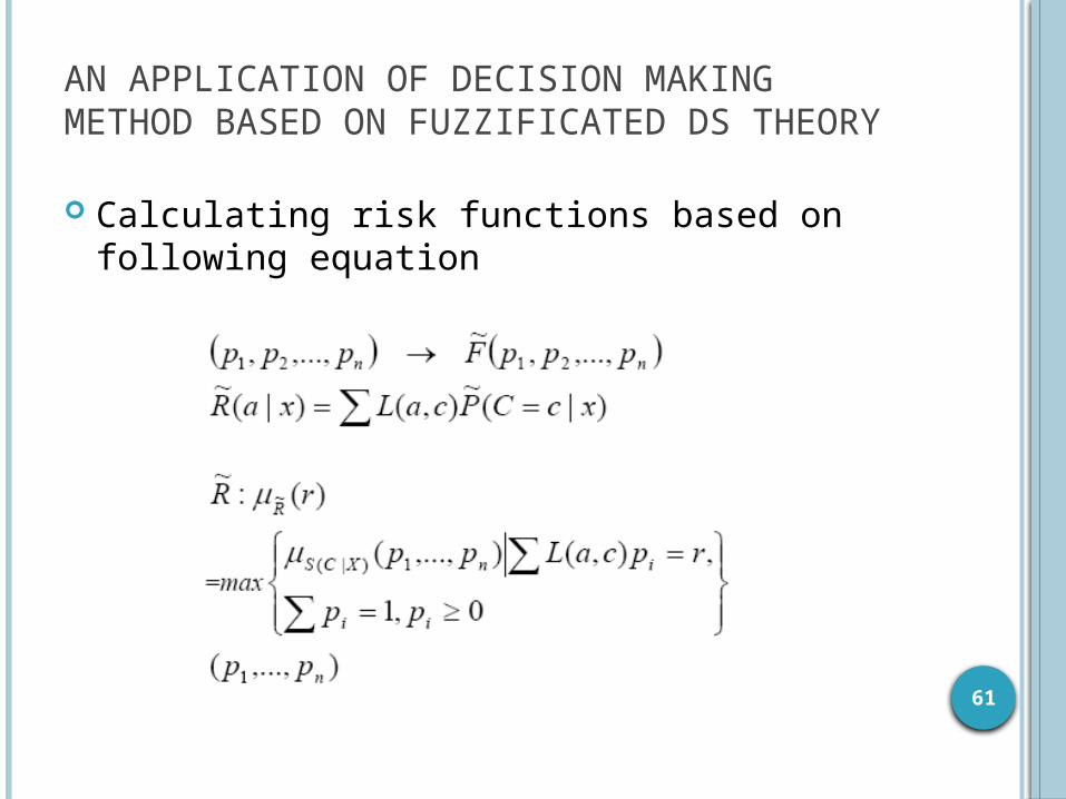
AN APPLICATION OF DECISION MAKING METHOD BASED ON FUZZIFICATED DS THEORY

Calculating risk functions based on following equation

62

AN APPLICATION OF DECISION MAKING METHOD BASED ON FUZZIFICATED DS THEORY a. Fuzzy set of risk function values for benign

prediction b.Fuzzy set of risk function values for

malignant prediction

63

AN APPLICATION OF DECISION MAKING METHOD BASED ON FUZZIFICATED DS THEORY The final step

rejecting uncertainties (fuzzyness and ignorance) to obtain a scalar value

These answers are calculated by

64

THANKS

in the name of allah decision making by using the theory of evidence students: hossein shirzadeh,...

Documents

shafers evidence theory

theory proof of inviability4

chance densities

little idea

value of idea

ones degrees of belief

introductionbelief function

ones degree of belief