increasing sales forecast accuracy with technique adoption...
TRANSCRIPT
Postal Address: Visiting Address: Telephone: Box 1026 Gjuterigatan 5 +4636-10 10 00 551 11 Jönköping Sweden
Increasing sales forecast accuracy with
technique adoption in the forecasting
process
Adam Hill
Richard Orrebrant
Bachelor Thesis 2014
Industrial Engineering and Management, Logistics and
Management


Postal Address: Visiting Address: Telephone: Box 1026 Gjuterigatan 5 +4636-10 10 00 551 11 Jönköping Sweden
This bachelor thesis was performed at Jönköping School of Engineering within the subject of Industrial Engineering and Management, Logistics and Management. The authors are responsible for the stated results, opinions, and conclusions. Examiner: Eva Johansson Supervisor: Roy Andersson Scope: 15hp (Bachelor level) Date: 08/06/2014
Abstract
I
Abstract Purpose - The purpose with this thesis is to investigate how to increase sales forecast accuracy. Methodology – To fulfil the purpose a case study was conducted. To collect data from the case study the authors performed interviews and gathered documents. The empirical data was then analysed and compared with the theoretical framework. Result – The result shows that inaccuracies in forecasts are not necessarily because of the forecasting technique but can be a result from an unorganized forecasting process and having an inefficient information flow. The result further shows that it is not only important to review the information flow within the company but in the supply chain as whole to improve a forecast’s accuracy. The result also shows that time series can generate more accurate sales forecasts compared to only using qualitative techniques. It is, however, necessary to use a qualitative technique when creating time series. Time series only take time and sales history into account when forecasting, expertise regarding consumer behaviour, promotion activity, and so on, is therefore needed. It is also crucial to use qualitative techniques when selecting time series technique to achieve higher sales forecast accuracy. Personal expertise and experience are needed to identify if there is enough sales history, how much the sales are fluctuating, and if there will be any seasonality in the forecast. If companies gain knowledge about the benefits from each technique the combination can improve the forecasting process and increase the accuracy of the sales forecast. Conclusions – This thesis, with support from a case study, shows how time series and qualitative techniques can be combined to achieve higher accuracy. Companies that want to achieve higher accuracy need to know how the different techniques work and what is needed to take into account when creating a sales forecast. It is also important to have knowledge about the benefits of a well-designed forecasting process, and to do that, improving the information flow both within the company and the supply chain is a necessity. Research limitations – Because there are several different techniques to apply when creating a sales forecast, the authors could have involved more techniques in the investigation. The thesis work could also have used multiple case study objects to increase the external validity of the thesis. Key words – Sales forecast, Forecast accuracy, Time series, Qualitative forecast, Forecasting process

Content
II
Content
1 Introduction..................................................................................... 1 1.1 Background .................................................................................................................................... 1 1.2 Problem description ................................................................................................................... 2 1.3 Purpose and research questions ........................................................................................... 4 1.4 Delimitations ................................................................................................................................. 4 1.5 Outline .............................................................................................................................................. 5
2 Methodology .................................................................................... 7 2.1 Work process................................................................................................................................. 7 2.2 Approach ......................................................................................................................................... 8 2.3 Case study ....................................................................................................................................... 8 2.4 Data collection .............................................................................................................................. 9 2.5 Analysis of data.......................................................................................................................... 11 2.6 Reliability ..................................................................................................................................... 12 2.7 Validity .......................................................................................................................................... 12
3 Theoretical framework ............................................................. 15 3.1 Link between research questions and theory .............................................................. 15 3.2 Forecast ........................................................................................................................................ 16 3.3 Forecasting process ................................................................................................................. 17 3.4 Forecast accuracy ..................................................................................................................... 18 3.5 Qualitative techniques ............................................................................................................ 21 3.6 Time series .................................................................................................................................. 25
4 Empirical data .............................................................................. 31 4.1 Case company ............................................................................................................................. 31 4.2 The case company’s forecasting process ........................................................................ 32 4.3 Current measurement of accuracy .................................................................................... 34
5 Time series tool ........................................................................... 35
6 Analysis of empirical data ........................................................ 39 6.1 The case company´s forecasting process ........................................................................ 39 6.2 Current measurement of accuracy .................................................................................... 40 6.3 Time series compared to qualitative sales forecast ................................................... 40
7 Recommended approach to forecasting ............................. 45 7.1 Forecasting process ................................................................................................................. 45 7.2 Accuracy measurements........................................................................................................ 46
8 Discussion and conclusion ....................................................... 49 8.1 Result ............................................................................................................................................. 49 8.2 Methodology discussion ........................................................................................................ 55 8.3 Conclusions ................................................................................................................................. 58 8.4 Future studies ............................................................................................................................ 59
Bibliography ................................................................................................ 61
Appendixes .................................................................................................. 67
Content
III
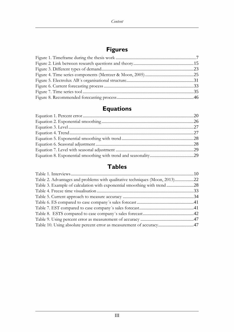
Figures
Figure 1. Timeframe during the thesis work .................................................................... 7
Figure 2. Link between research questions and theory ................................................... 15
Figure 3. Different types of demand .............................................................................. 23
Figure 4. Time series components (Mentzer & Moon, 2005) ......................................... 25
Figure 5. Electrolux AB´s organisational structure......................................................... 31
Figure 6. Current forecasting process ............................................................................ 33
Figure 7. Time series tool .............................................................................................. 35
Figure 8. Recommended forecasting process ................................................................. 46
Equations Equation 1. Percent error .............................................................................................. 20
Equation 2. Exponential smoothing .............................................................................. 26
Equation 3. Level .......................................................................................................... 27
Equation 4. Trend ......................................................................................................... 27
Equation 5. Exponential smoothing with trend ............................................................. 28
Equation 6. Seasonal adjustment ................................................................................... 28
Equation 7. Level with seasonal adjustment .................................................................. 29
Equation 8. Exponential smoothing with trend and seasonality ..................................... 29
Tables Table 1. Interviews ........................................................................................................ 10
Table 2. Advantages and problems with qualitative techniques (Moon, 2013) ................ 22
Table 3. Example of calculation with exponential smoothing with trend ....................... 28
Table 4. Freeze time visualisation .................................................................................. 33
Table 5. Current approach to measure accuracy ............................................................ 34
Table 6. ES compared to case company´s sales forecast ................................................ 41
Table 7. EST compared to case company´s sales forecast .............................................. 41
Table 8. ESTS compared to case company´s sales forecast ........................................... 42
Table 9. Using percent error as measurement of accuracy ............................................. 47
Table 10. Using absolute percent error as measurement of accuracy .............................. 47
Introduction
1
1 Introduction
This chapter starts by describing the background and the main motives for the thesis. After the background, a more detailed description of the problem is presented. This is followed by the purpose of the thesis along with two research questions. Delimitation then describes the focus area of the thesis and the outline describes the structure of the thesis.
1.1 Background
The competition on the global market is constantly increasing due to more companies. This leads to a wider range of products and services and higher requirements from customers. Because of this, companies try to make the processes more efficient to become more successful than competitors and gain more market-share (Cheung et al., 2004). One way to make a company efficient is to ensure that all departments’ strategies interlock with each other to form a shared strategy. It is the way that manufacturing, marketing, finance, research & development, in other words, all departments, work together that creates an advantage over competitors (Miltenburg, 2005). For a company to achieve competitive advantages a plan and competitive strategy needs to be formed, to successfully compete against competitors (Miltenburg, 2005). Companies often begin with forecasting customers demand to be able to form a plan; creating a sales forecast (Herbig et al., 1993; Mentzer & Moon, 2005). Mentzer and Moon (2005) defines a sales forecast as “a projection into the future of expected demand, given a stated set of environmental conditions”. A sales forecast can therefore be explained as a way of using different factors (e.g. sales history, sales promotion, seasonality, and so on) to predict future sales and then use information from the forecast to develop plans for resources and capacity to meet the demand in the best possible way (Herbig et al., 1993; Jonsson & Mattson, 2011; Mentzer & Moon, 2005). A sales forecast can also be used in significant managerial decision-making within companies (Herbig et al., 1993; Lee, 2000; Mentzer & Moon, 2005). If managers get more reliable information about future demand the simpler is the decision-making about customer requirements going to be (Herbig et al., 1993; Mentzer & Moon, 2005). For companies to be able to share the information for the sales forecast, a well-designed forecasting process must exist. A well-designed forecasting process helps the company share information within the company, not just the outgoing data but also information about which data to use when forecasting, for example: marketing activities, market dynamics, consumer behaviour, and so on (Danese & Kalchschmidt, 2011). With a well-designed forecasting process companies can increase the sales forecast accuracy; by ensuring that the ingoing data is as accurate as possible (Ramanathan, 2012). Because of the wide range of products, customers’ expectations on companies are increasing. Those expectations have today led to customers expecting products to
Introduction
2
be available at the right place, in the right quantity, at the right time. It may therefore be necessary for companies with delivery time as a competitive advantage to produce against a sales forecast instead of, for example incoming orders, to ensure that supplies are available (Arnold et al., 2007). A sales forecast does not only affect the production unit in a company but also affects the sales department, marketing & finance, operations & inventory, in other words it affects the whole company (Gilmore & Lewis, 2006; Mentzer & Moon, 2005). Different departments need different kind of information from the sales forecast (e.g. operation & inventory needs information about “units” and financial & marketing needs information about “dollars”) it is therefore important to transform the demand into different units (Mentzer & Moon, 2005). Unfortunately it is hard to predict the future and therefore are sales forecasts almost always wrong (Herbig et al., 1993). Because of this, and the sales forecasts impact on the company, most companies focus is in improving the sales forecast accuracy (Danese & Kalchschmidt, 2011; Linderman et al., 2003; Mentzer & Moon, 2005). An accurate sales forecast has the potential to make a company successful. If the forecast is accurate the company knows how many, and when, products are needed. From this information plans can be developed for production, when the products or services need to be ready for delivery, what is needed to be purchased and how much and so on (Huang et al., 2010; Mentzer & Moon, 2005; Vollmann et al., 1992). In other words, the more accurate a forecast is, the more are the benefits from it.
1.2 Problem description
Because sales forecasts are mostly wrong it is important for companies to make the forecast as accurate as possible, to minimize potential consequences as an inaccurate purchase of material or incorrect scheduling of recourses (Arnold et al., 2007; Currie & Rowley, 2010; Herbig et al., 1993). The more accurate the data is that is used to make the forecast, the more accurate is the outgoing data going to be (Lawrence et al., 2000). There are different factors for the complexity of the ingoing data in a forecast; one reason is consumer behaviour. The complexity of consumer behaviour is because it is difficult to foresee, but predictions can be made from the right kind of information (Currie & Rowley, 2010; Jonsson & Mattson, 2011). Another factor that also needs to be taken into consideration when creating a sales forecast is different types of demand that flow through the supply chain. A company is affected differently by these types of demand depending on the structure of and the company´s localisation in the supply chain. To be able to make accurate predictions of future demand the company must understand the differences and how to take them into account (Mentzer & Moon, 2005). The data that the forecast is based on depends on what the company´s purpose of the forecast, resources available and accuracy needed. Other factors that might be needed to take into consideration are: sales promotions, seasonality, and general economic conditions, among others (Lysons & Farrington, 2012).

Introduction
3
Not only is a forecast important for all industries but also in all parts of a company. All departments have an interest in a well-made forecast to base decisions on (Herbig et al., 1993). Although, with that in mind there have been surprisingly little work on the understanding of how to manage a forecasting process (Mentzer et al., 1999; Moon et al., 2003). Since the whole company finds use in an accurate sales forecast, companies should have a well-designed forecasting process so that information regarding the sales forecast flows easily within the company (Danese & Kalchschmidt, 2011). Most researchers have focused on improving the forecasting techniques and try to adopt different techniques to increase the sales forecast accuracy, instead of improving the forecasting process (Danese & Kalchschmidt, 2011). Mentzer and Moon (2005) mention that to increase the accuracy, information flow about different factors that are going to affect the sales forecast and also that the “right” data used for the forecasting techniques is needed to increase the accuracy. This is difficult to achieve without a well-designed forecasting process. According to Hoshmand (2010) many companies are only using qualitative techniques; where judgments of sales are made to create a sales forecast. Companies do not want to put an effort or do not see the benefit from quantitative techniques; using historical data, such as sales history, to create a sales forecast. Moon (2013) mentions that it can be both costly and time consuming to rely only on qualitative techniques when forecasting. Companies should therefore evaluate how to adopt different forecasting techniques to increase the sales forecast accuracy.
Introduction
4
1.3 Purpose and research questions
As mentioned, the most substantial problem with a sales forecast is that it is almost always wrong. It is therefore important to eliminate as many uncertainties as possible and improve the overall accuracy of the sales forecast, so that eventual consequences can be reduced. The inaccuracy can also be a problem when companies only rely on qualitative techniques and do not have an adequate base for predicting future sales and the forecast will not be as accurate as wanted. The purpose of this thesis is therefore to:
Investigate how to increase sales forecast accuracy As mentioned in the background, a well-designed forecasting process can increase the accuracy. It also contributes to a good information flow, regarding the sales forecast, within the company that helps the company to form plans and strategies. It is therefore important to find out what should be taken in regard when developing a well-designed forecasting process. The authors have thus come up with the first question to answer:
1. What should be considered when developing a forecasting process? For a company to be able to increase the sales forecast accuracy even more, knowledge about different techniques is needed and how the techniques can be combined to achieve higher accuracy, which leads to research question number two:
2. How can a combination between time series and qualitative techniques be used to increase the accuracy?
These two questions are needed to fulfil the purpose of the thesis. Question one is needed to find out how a forecasting process can be designed and managed, and question two to see how different techniques are used when forecasting and how the techniques can be combined to increase the accuracy of a forecast. When the two questions have been answered the purpose will be fulfilled.
1.4 Delimitations
There are a lot of different forecasting techniques that can be combined. Because of the study´s timeframe the authors decided to focus on two types of forecasting techniques; time series and qualitative techniques. The choice for these two is because time series is mentioned as a good forecasting technique by several researchers and the use of qualitative techniques is needed when creating a sales forecast from time series. There are also a lot of different time series techniques, and most of these techniques are relatively complex and do not provide a more accurate forecast than a simpler technique (Mentzer & Moon, 2005). This thesis will only focus on
Introduction
5
three well-known time series techniques that provide a good accuracy according to the theory. Because different qualitative techniques are almost the same, where professional individuals make judgments of the future, this thesis will not mention any specific qualitative technique. It will only mention qualitative techniques as a whole.
1.5 Outline
In the introduction of the thesis, a background of forecasts can be found describing why a forecast is important, what it can be used for and different techniques for forecasting. After the background there is a problem description where the authors describe different problem areas of forecasting and why the problems should be considered. After that the purpose of the thesis is defined along with two research questions needed to fulfil the purpose. The introduction ends with a presentation of the thesis delimitations. In the second chapter, methodology, the approach and methods used by the authors are presented. How theory and empirical data was collected, how the data has been analysed and also applied through a case study. In addition, a description of how the work will maintain a good validity and reliability is also presented. In the beginning of the third chapter there is a description of theory has been used for the two research questions. After that the concept of forecasting and forecasting process is described in more detail, what is meant with accuracy of a forecast and how it can be measured. The chapter ends with the highlighting of qualitative technique and different time series techniques that can be used when creating a forecast. The fourth chapter is about the empirical data that was collected for the thesis. To support the result of the thesis the authors chose to do a case study. This chapter describes the case company the authors have collaborated with. It also describes the forecasting process and forecasting techniques that are used by the case company. The fifth chapter presents a tool the authors developed for forecasting sales by using time series techniques. There is a description of the tool that was created and how it can be used. Different advantages and disadvantages regarding the tool are also specified in this chapter. This chapter is needed to understand the comparison between time series and qualitative techniques that is going to be presented later. In the sixth chapter the authors analyse the empirical data collected through the case study. The current forecasting process used by the case company is analysed as well as the way the case company measure and determine sales forecast accuracy. There is also an analysis of the comparisons between forecasts the tool created compared to the case company’s qualitative forecasting technique. These
Introduction
6
analyses are then used to come up with improvements areas and the foundations to the answers of the research questions. In chapter seven the authors provide recommended approaches from the analysis of the empirical data. By comparing the theoretical background with the empirical data the authors present own recommendations for a new forecasting process and alternative ways to determine accuracy. Chapter five to seven is the result thesis work. The eighth chapter presents the discussion of the thesis work. First the result will be discussed in form of how the two research questions have been answered. There is also a methodology discussion where the authors evaluate the way the thesis work has been conducted. The chapter ends with the authors´ own conclusions and areas for future studies within the subject.
Methodology
7
2 Methodology
This chapter describes the procedures used to fulfil the purpose of the thesis. It also describes how theory and empirical data was collected, how the data has been analysed and also applied through a case study. In the end the reliability and the validity of the thesis is presented. The chapter starts with an introduction on how the work process was conducted.
2.1 Work process
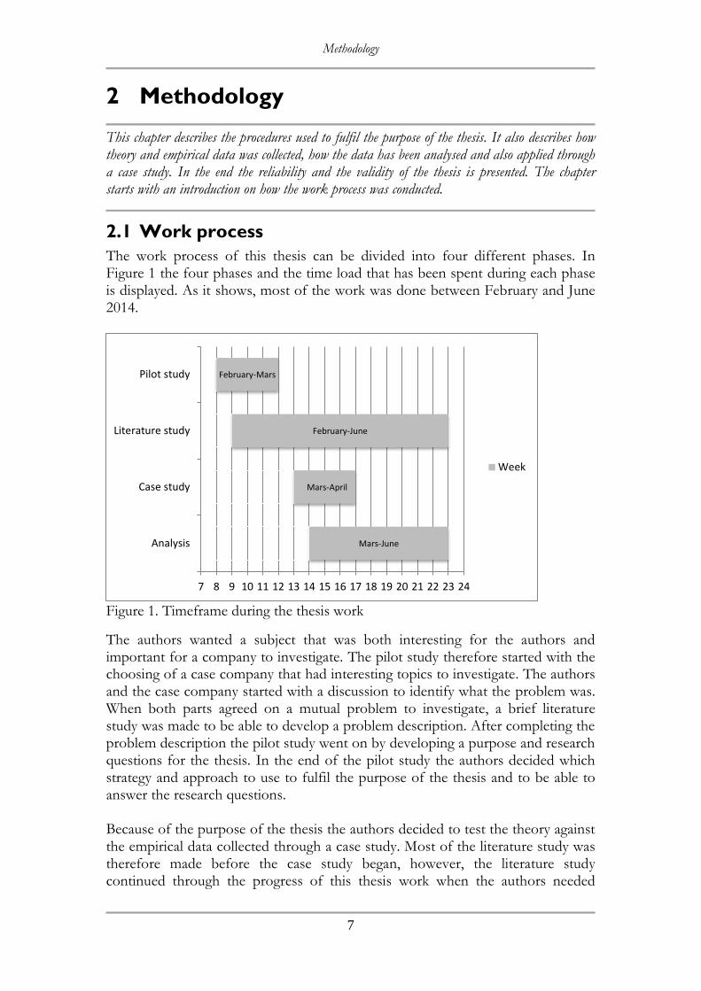
The work process of this thesis can be divided into four different phases. In Figure 1 the four phases and the time load that has been spent during each phase is displayed. As it shows, most of the work was done between February and June 2014.
Figure 1. Timeframe during the thesis work
The authors wanted a subject that was both interesting for the authors and important for a company to investigate. The pilot study therefore started with the choosing of a case company that had interesting topics to investigate. The authors and the case company started with a discussion to identify what the problem was. When both parts agreed on a mutual problem to investigate, a brief literature study was made to be able to develop a problem description. After completing the problem description the pilot study went on by developing a purpose and research questions for the thesis. In the end of the pilot study the authors decided which strategy and approach to use to fulfil the purpose of the thesis and to be able to answer the research questions. Because of the purpose of the thesis the authors decided to test the theory against the empirical data collected through a case study. Most of the literature study was therefore made before the case study began, however, the literature study continued through the progress of this thesis work when the authors needed
Mars-June
Mars-April
February-June
February-Mars
7 8 9 10 11 12 13 14 15 16 17 18 19 20 21 22 23 24
Analysis
Case study
Literature study
Pilot study
Week

Methodology
8
additional data. The literature study was the part that required the most attention to complete, the main reason for that was the selection of time series and qualitative techniques to use in the thesis. Because of the wide range of techniques it was time consuming to identify the techniques that would be appropriate for the subject. Besides the identification of techniques, a theoretical framework was designed for the authors to be able to apply the different forecasting techniques on the case company. When enough theory had been gathered for the analysis of the case company´s forecasting process, the case study began. As mentioned, the main goal of the case study was to analyse how the forecasting techniques, in research question two, works in reality. This phase was the most intensive phase of the thesis work due to that there were several techniques to test within a short timeframe. All empirical data gathered during the case study was continuously analysed.
2.2 Approach
To answer the research questions the authors first gathered information about different theories and then compared these with the empirical data collected. When the authors found out that theory was missing to fulfill the comparison between theories and empirics the authors went back to study more theories. This process, when the authors went between theory and empirics, continued through the whole thesis work. According to Olsson and Sörensen (2011) this is an abductive approach. This approach was chosen because the authors wanted to see if well-known theories could be applied in real life situations. The authors also wanted to get own opinions about the subject and a comparison between theoretical and empirical data was therefore the best approach. To be able to fulfil the purpose of the thesis and answer both research questions a mixture of a qualitative and a quantitative methodological approach has been used. For the authors to be able to analyse the case company’s sales forecast, quantitative data, such as historical sales numbers, has been collected from the company. Several interviews have also been conducted to gather qualitative information about the case company’s forecasting process and what the company believes is important to take into consideration when creating a sales forecast. By mixing these two types of methodological approaches the authors got a better framework to be able to perform an analysis of the case company. According to Holme and Solvang (1997) this mixture is an appropriate approach because using a qualitative approach is a good foundation to a quantitative approach.
2.3 Case study
A case study is a research study that focuses on gathering information from a single or multiple case study objects, to get an increased understanding of a subject (Eisenhardt, 1989). A case study can be both qualitative with observations and interviews and quantitative with studies of documents (Eisenhardt, 1989; Gustavsson, 2004). Depending on the subject of the thesis work the mixture of
Methodology
9
these two methods can differ. Qualitative methods are however the most common when performing a case study (Gustavsson, 2004). Applying the theory gathered to answer the research questions to a real case is an advantage of using a case study, since it increases the validity of the thesis (Benneth, 2003). The case study was also a good compliment to the literature study for areas where the literature was inadequate. The authors chose a single case study object, Electrolux AB in Bangkok, Thailand, and the reason was so the authors could analyse a specific case more thorough instead of doing a general study. The reason for choosing Electrolux AB was because of an interesting topic for the thesis work; to evaluate the company’s technique used when sales forecasting. Electrolux AB´s forecasting process was missing a theoretical base for the technique used when forecasting and the company was looking for areas to improve, to increase the accuracy of the sales forecast. Because of the continuous increase of demand of household appliances in Southeast Asia, Electrolux AB´s sales forecast accuracy was crucial to improve. The year-to-year variation in demand sets the requirement of an accurate forecast to estimate future demand. The forecast is also essential to be able to plan the production in one of the company´s largest manufacturing facilities for refrigerators located in Rayong, Thailand. The factory not only provides and distributes goods to Southeast Asia but also globally and an accurate sales forecast is therefore a necessity. Through the case study the authors got a better insight in how a company´s forecasting process may be designed and what kind of forecasting techniques are used. By analysing these techniques the authors came up with areas to improve to increase the sales forecast accuracy.
2.4 Data collection
In order to answer the research questions, different types of data was collected. A literature study was made to get a theoretical framework for the thesis. The literature study was then supplemented with a case study where data was collected by interviews and documents.
2.4.1 Literature study
A literature study was made to get a better understanding about the subject and to be able to test theory against reality. During the literature study different techniques and forecast accuracy was the main focus, but also how the work around the creation of a sales forecast was of interest, to be able to find information about the concept of “forecasting”. The main source to find literature about the subjects was from Jönköping University’s library database. Most of the literature consisted of scientific articles and textbooks. The keywords the authors used were forecast, sales forecast accuracy, forecasting techniques, time series, qualitative forecast, developing a sales forecast, and forecasting process. The authors compared the theory from the different scientific articles and textbooks to find a common

Methodology
10
pattern between the articles and textbooks. The authors could then sort out which theory to use for the thesis.
2.4.2 Interviews
The interviews were conducted to gain an understanding of the problem and to get a more detailed insight in the case company´s forecasting process. It was also a necessity to conduct interviews to understand the documents that were handed to the authors for analysis. Most interviews had a semi-structured approach with open-ended questions to get a wider range of answers. According to Yin (2011) open-ended questions is a good approach when the questions cannot limit the answers but still get the main subject answered. The authors wanted the interviews to be more like discussions to get a more personal interview with the respondents, thereof the choice of approach. Before the first two interviews only a few questions were prepared for the respondents. This was because the authors wanted the interviews to be more like discussions to get a better understanding of the problem the case company believed to have, but also to discuss the purpose of the thesis. For the other interviews more questions were prepared to be sure that the purpose of the interview was answered, Appendix 1 contains the same questions to all the involved departments and Appendix 2 contains only question to supply chain regarding what the forecasting techniques look like. During the interviews, one of the authors did most of the questioning and discussing while the other took notes, apart from a few situations where a joint discussion was used and the information was compiled afterwards. Table 1 shows the respondents, the date when the interview took place, length of the interview, and the interviews main subject. The roles of the respondents are Financial Controller (FC), Supply Chain Manager (SCM), Assistant Supply Chain Manager (ASCM), employee involved in the forecasting process from the sales department (Sales) and employee involved in the forecasting process from the marketing department (Marketing). Table 1. Interviews
Date Role Length/min Subject
2014-02-20 FC, SCM, ASCM 60 Case company´s problem
2014-03-06 SCM, ASCM 60 The thesis´s purpose, scope, and time schedule
2014-03-28 ASCM 60 Case company´s forecasting technique
2014-04-09 ASCM 90 Walkthrough of forecasting process step-by-step
2014-04-09 SCM 20 Organisational structure
2014-04-09 SCM 40 Supply Chain´s view on sales forecasting
2014-04-09 Sales 30 Sales´s view on sales forecasting
2014-04-09 Marketing 30 Marketing´s view on sales forecasting
2014-04-18 SCM, ASCM 30 Calculation of accuracy

Methodology
11
As Table 1 shows, interviews have been used to gather information for both research questions. For research question one, interview four and six to nine have been conducted to gather information, and for research question two interview three and nine have been conducted to gather information. Interview five was conducted so the authors could get a more detailed view on the case company´s organisation.
2.4.3 Documentation
To be able to sort out information about different aspects of how the case company works with forecasts, different types of documents have been gathered with data about the forecasting process and sales history. First the authors needed information about how the forecasting process is designed to get a picture of what more kind of information would be needed and what was needed to be improved. Documents about the process were gathered and also explained during the fourth interview. The authors then also needed information about sales history that was used for the testing of different forecasting techniques. The sales history-document was a Microsoft Excel-file with the sales history for a specific product group the last five years. The sales history was further a necessary part when developing the time series tool since it uses sales history to estimate future sales. Documents regarding forecast history were also needed to see how well the case company’s previous forecasts had performed, but it was also needed to be able to compare the authors´ forecasts with the case company´s. By studying these types of documents the authors got a basis of how the case company works with forecasts and how the previous performance has been.
2.5 Analysis of data
Analysis of data was a continuous process that continued until it all was summarised. With the risk of judging any forecasting technique favourably most of the theoretical framework was, as mentioned, done before the empirical study began. This way the authors got an own view of different forecasting techniques before the investigation of the technique being used at the case company began. With this approach the authors could decide which techniques to include in the thesis work without regard to the one being used. To make sure that no data was misinterpreted or lost it was summarised directly after the collection while it was still new and therefore more easily studied (Jacobsen, 2002). The data collected was also compiled and simplified which makes it easier for the reader to understand (Larsen, 2007; Patel & Davidsson, 2003). The empirical data collected was compared with the theoretical and analysed to achieve a result, recommendations and conclusion. The authors also did an own evaluation of the current forecasting process used by the case company to be able to answer research question one. The different activities in the process were analysed to get an understanding of what kind of information was being used to find eventual improvement areas. The authors also did interviews with employees involved in the forecasting process to get the
Methodology
12
employees´ point of view and a more thorough understanding of the inputs used when forecasting. From the collected information about the forecasting process being used the authors compared the current inputs used to the theoretical data collected and came up with ideas for improving the process. To be able to answer research question two, the authors have developed a tool to make forecasts with time series. The tool´s forecast could then be analysed against the case company´s qualitative forecast to see how time series and qualitative techniques could be combined. The needed documents of sales history and forecast history were sorted and simplified in Microsoft Excel right after it was collected, for an easier analysis. The data was then inserted into the developed tool. The authors then reviewed the performance of different techniques in regard to the actual sales for the same period provided by the sales history-documents. The case company’s actual performance for the same time period was also calculated and compared to the authors own to determine which technique would have been the most accurate. The same calculations were done for multiple time periods selected from the sales history to strengthen the result of the comparisons.
2.6 Reliability
Reliability is about the trustworthiness of the measurements, that what is measured is measured correctly (Bell, 2006; Patel & Davidsson, 2003). High reliability also means that the thesis work can be repeated and will achieve similar results as the original thesis work (Patel & Davidsson, 2003). For the thesis to attain a high reliability, interviews with different employees with various positions in different departments (supply chain, marketing, and sales) have been conducted to gain a wider range of understanding of the problem area. Some employees have also been interviewed more than once to make sure that data from previous interviews have been correct. Data has also been collected through a literature study on different theories regarding the subject. According to Yin (2003) data collection from different sources, so called triangulation, can give a greater understanding of the problem area. The authors have attached the interview questions, regarding the sales forecast, that were used during interviews with employees from marketing, sales, and supply chain, to facilitate that a similar thesis work can achieve a similar result. The authors have also made sure that the methodology was described in detail and analysed so others can see how the thesis work has been performed and what the authors thought about the chosen approach.
2.7 Validity
There are two types of validity, internal and external validity. Internal validity means that the right things are measured to achieve the purpose, while external validity describes whether the thesis is generalizable or not to other similar cases (Merriam, 1994; Patel & Davidsson, 2003)
Methodology
13
By discussing with the case company in the pre-study regarding what the problem was, the authors got a picture of what needed to be measured. When the problem was identified a background and problem description was made and from these a well-defined purpose could be made. The authors developed two research questions with motivations why the questions were needed for the thesis to fulfil its purpose. By discussing with the case company and having a well-defined purpose with subsequent research questions the authors were able to identify what information would be needed. To be able to further increase the internal validity the authors continuously held a discussion with the case company throughout the work to ensure that the right things were measured. To be able to increase the external validity discussions were conducted with the case company regarding the recommended forecasting process that was developed. By getting the forecasting process reviewed by the case company and get it approved can increase the external validity (Persson, 2003). The authors have also compared well-known theories about the subject with the empirical data from the case company to see how theories reflect the reality. The authors have made a detailed description of the case study in the thesis to show the forecasting process that the case company is currently using so readers can see how the current situations is.

Theoretical framework
15
3 Theoretical framework
This chapter contains the theoretical components that form the basis of the thesis and will later be applied to the empirical data. The theoretical framework will start with a description of how each theory is connected with each research question. The theories are divided into five different main categories; forecast, forecasting process, forecast accuracy, qualitative techniques, and time series. Each category has smaller chapters that will present more detailed theory about each main category.
3.1 Link between research questions and theory
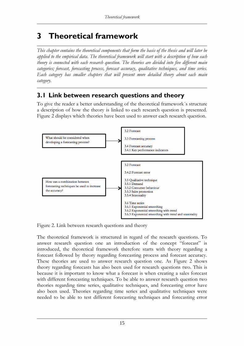
To give the reader a better understanding of the theoretical framework´s structure a description of how the theory is linked to each research question is presented. Figure 2 displays which theories have been used to answer each research question.
Figure 2. Link between research questions and theory
The theoretical framework is structured in regard of the research questions. To answer research question one an introduction of the concept “forecast” is introduced, the theoretical framework therefore starts with theory regarding a forecast followed by theory regarding forecasting process and forecast accuracy. These theories are used to answer research question one. As Figure 2 shows theory regarding forecasts has also been used for research questions two. This is because it is important to know what a forecast is when creating a sales forecast with different forecasting techniques. To be able to answer research question two theories regarding time series, qualitative techniques, and forecasting error have also been used. Theories regarding time series and qualitative techniques were needed to be able to test different forecasting techniques and forecasting error

Theoretical framework
16
was needed when calculating if the techniques were providing an accurate sales forecast.
3.2 Forecast
The first step in achieving an effective production is to make decisions on how much that is needed to be produced during certain period of time. Companies therefore need to make predictions of the products future demand. These predictions are then used for the planning, budgeting and scheduling of the companies resources. These kinds of predictions are also known as sales forecasts (Bovee et al., 2006). Regardless of industry, whether the company is a manufacturer, wholesaler, retailer or service provider, it is important to effectively forecast demand. This helps companies identify market opportunities, increase customer satisfaction, reduce inventory and obsolescence products and make scheduling more effective (Linderman et al., 2003; McIntyre et al., 1993). Because of this, forecasting is an important part of all industries when it comes to business planning and management (Armstrong et al., 1997; Fildes & Hastings, 1994) and is in many cases what the basis of the corporate strategy is built upon (Mentzer et al., 1999). Work with the management of forecasting processes includes decision-making about information gathering and tools, in other words; what information should be collected and how it should be used. It also includes organisational issues as to which department is responsible for creating the forecasts. Decisions also need to be taken in regard to the cooperation of information flow, both between the companies departments but also within the supply chain. Information from multiple sources can be used to improve the accuracy of the forecast (Fildes & Hastings, 1994; Fisher et al., 1994; Remus et al., 1995). This means that; to improve the understanding of how to reduce forecasting miscalculations companies must study the connections between forecasting techniques and different factors (Danese & Kalchschmidt, 2011). Despite the advanced tools available the outgoing data can, however, only be as accurate as the ingoing data. It is common that companies spend too much time on advanced tools, when focus instead should be on processes, procedures, and educating forecasters (the developers of a forecast) (Lawrence et al., 2000). It is important that all departments provide input for the forecast and that all essential data is regarded when making decisions (Gilmore & Lewis, 2006; Mentzer & Moon, 2005). A common problem in the making of a forecast is that not all departments realise the advantages and are therefore not interested in being part of the forecast creation. Thus is it important to make the departments understand in what way each department can benefit from an accurate forecast. A difficult task is also to balance it evenly so that the forecast does not become too extensive. It is important to acknowledge the differences between core needs of sales and wants of sales. The process of forecasting is often overcomplicated because of these differences (Gilmore & Lewis, 2006).
Theoretical framework
17
A source for significant cost differences between companies is not unusually because of the forecast. The main reason for this is the difference between the forecasts’ accuracy. There are two types cost problems that are results from an inaccurate forecast. The first one is if there is an over-forecast that results in overstock and obsolescence products and the second one is if there is an under-forecast; which means that the company do not have enough products and the cost of lost sales increases (Dalrymple, 1987; Huang et al., 2010; Lawrence et al., 2000; Mahmoud et al., 1988). A sales forecast is therefore an important part of a company’s profitability and market share (Huang et al., 2010; Lee, 2000). Forecasts are also of significance in management decisions as they are explicitly or implicitly based on predictions about the future (Herbig et al., 1993; Lee, 2000). For a business to survive it is important to reach the customers at least as fast as competitors. The more accurate manager decisions about the future are, the more successful will companies be when adapting to different situations (Herbig et al., 1993). It is therefore important that all decisions in a company or even the supply chain are based on a single, shared and accurate forecast (Mentzer & Bienstock, 1998). Technologies in forecasting have developed from having the same technique for all products to instead using technology that adapts techniques for each product in order to achieve higher accuracy (Mentzer & Kahn, 1997; Mentzer & Schroeter, 1993). However, if compared to other areas within the company, the performance of forecasts has improved remarkably little, even among more successful companies (Mentzer et al., 1999; Moon et al., 2003). There is much research and theory that have contributed to developing the understanding of how to create appropriate techniques to make forecasts. The understanding of what actually affects forecasts is, however, deficient in many companies (Mentzer et al., 1999; Winklhofer et al., 1996). The research of forecasts now focuses more on how to take the knowledge gained about forecasting and implement that in companies to improve forecasts (Moon et al., 2003). So as attention of the importance about forecasting increases, focus is moved from having focused mainly on different techniques, to focusing on the forecasting process (Bunn & Taylor, 2001).
3.3 Forecasting process
Previous studies have focused on an adoption between different techniques, both quantitative and qualitative, to achieve higher accuracy. Moon et al. (2003) mean that technique adoption will not guarantee a good accuracy and therefore should companies also focus on how the forecasting process is managed and organized. The main objective of a forecasting process is to maintain a good information flow within the company and also organize the work around the creation of the sales forecast (Danese & Kalchschmidt, 2011).
Theoretical framework
18
According to Danese and Kalchschmidt (2011) a forecasting process can be divided into four different steps information-gathering and tools (what information should be collected and how it should be collected), organizational (who should be in charge of forecasting and what roles should be designed), interfunctional and intercompany (using different sources of information within the company or supply network and a joint elaboration of forecasts), and measurement of accuracy (using the proper metric and defining proper incentive mechanisms). These steps should always be under continuous improvement to ensure a high sales forecast accuracy. A company that has a well-designed forecasting process provides a better opportunity to understand market dynamics and consumer behaviour, reduce uncertainty of future events, and provide the company´s departments with useful analyses and information (Danese & Kalchschmidt, 2011). As mentioned previously, the companies’ departments should rely on one shared sales forecast, the forecasting process is therefore important when making sure that the information flow regarding the sales forecast is efficient. One way to improve the forecasting process is to have one shared database within the company to gather and share information regarding the sales forecast (Moon et al., 2003). If a company can develop a well-designed forecasting process and use an adoption between different techniques, the company will facilitate the work to achieving higher sales forecast accuracy (Danese & Kalchschmidt, 2011).
3.4 Forecast accuracy
Herbig et al. (1993) states that “Forecasts are almost always wrong.”. An important part of forecasting demand is therefore making sure forecasts are as accurate as possible (Currie & Rowley, 2010; Herbig et al., 1993). Forecast accuracy is important as substantial errors often affect companies performance negatively, especially costs and delivery time (Enns, 2002; Fisher & Raman, 1996; Zhao & Xie, 2002). An accurate forecast enables the short- and long-term predictions of necessary capacity that in return contributes to better utilization (Danese & Kalchschmidt, 2011). This leads to the company being able to provide the customer with the product at the point of order. The product can then be provided at the right time, at the right place, in the right quantity, which increases the overall level of service towards customers (Enns, 2002; Kalchschmidt et al., 2003). A forecast, when being accurate, estimates future economic activity and can be useful when determining a course of action and when forming a corporate strategy for uncertain occurrences. However, should the forecast be inaccurate it can bankrupt or at the very least put a company behind its competitors. In most cases when increasing the precision of a forecast a result is a higher expense in technologies and increased time for the gathering of necessary data. Thus is a risk by improving the forecast´s accuracy that it will become costly and take long time (Herbig et al., 1993). Mentzer and Moon (2005) suggests that expenses for

Theoretical framework
19
improving the accuracy of a forecast should be viewed as a return on investment decision, where the return is seen as lower supply chain management costs and increased customer satisfaction. The more decisions that are based on a forecast the more important it is to increase the accuracy of it (Mentzer & Bienstock, 1998). Even though the forecasting technique affects the accuracy, improving the forecasting process can be more important. Studies show that regardless of the technique chosen for forecasting demand the inaccuracy is not necessarily because of the technique. Unorganised work with procedures and approaches can have a large impact on a forecast´s accuracy (Mentzer & Bienstock, 1998; Moon et al., 2003). Combining information and data from different parts of the company and supply chain can provide more certain information about future demand and thereby also lead to improved accuracy (Bartezzaghi & Verganti, 1995; Chen et al., 2000). The same is it with combining data about different products. Herbig et al (1993) found that forecasts based on categories or groups of products are often more accurate than forecasting a single product or model. To increase the accuracy of a forecast, companies constantly need to work with it and make continuous improvements (Bovee et al., 2006). Many factors, for example trends and consumer behaviour, cannot easily be predicted when forecasting sales and it is therefore important to consider that the longer the time horizon is for the forecast, the more inaccurate and unreliable are the predictions (Bovee et al., 2006; Herbig et al., 1993).
3.4.1 Key performance indicators
To determine whether a forecast is accurate or not an indicator for forecast accuracy is needed. Its purpose is to measure how accurate the forecast is and provide the company with information of the forecasts past or current performance. These types of indicators used to measure organisational performance are called key performance indicators (KPI’s). The KPI is a predetermined value of the wished or expected performance of an activity. This value is then compared to the outcome to determine whether the performance of the activity is acceptable (Parmenter, 2010). For example: a company measures the performance of the sales forecasts by determining the forecast´s accuracy and the predetermined indicator for forecast accuracy is set to 85 percent. The allowed difference between the forecasted sales and the actual sales of a product, for it to be considered as 85 percent accurate, is therefore: . It means that the forecasted sales are allowed to vary with as much as ± 15 percent, from 85-115 percent, of the actual sales to still be an accurate forecast. When the forecast varies with more than ±15 percent from the actual sales it is considered as inaccurate, this 15 percent variation will later be explained as forecasting error in chapter 3.4.2. By using KPI’s a company can determine whether the forecast is accurate or inaccurate.
Theoretical framework
20
To make the forecast as accurate as possible it is important to monitor the KPI’s regularly, preferably on a daily or weekly basis. If the circumstances affecting the outcome of the forecast are expected to remain it is important to make continuous updates to the forecast to increase the future accuracy (Parmenter, 2010).
3.4.2 Forecasting error
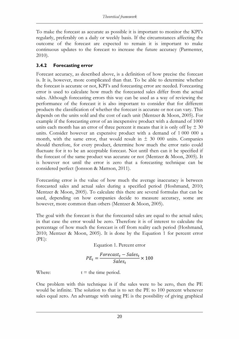
Forecast accuracy, as described above, is a definition of how precise the forecast is. It is, however, more complicated than that. To be able to determine whether the forecast is accurate or not, KPI’s and forecasting error are needed. Forecasting error is used to calculate how much the forecasted sales differ from the actual sales. Although forecasting errors this way can be used as a way of reviewing the performance of the forecast it is also important to consider that for different products the classification of whether the forecast is accurate or not can vary. This depends on the units sold and the cost of each unit (Mentzer & Moon, 2005). For example if the forecasting error of an inexpensive product with a demand of 1000 units each month has an error of three percent it means that it is only off by ± 30 units. Consider however an expensive product with a demand of 1 000 000 a month, with the same error, that would result in ± 30 000 units. Companies should therefore, for every product, determine how much the error ratio could fluctuate for it to be an acceptable forecast. Not until then can it be specified if the forecast of the same product was accurate or not (Mentzer & Moon, 2005). It is however not until the error is zero that a forecasting technique can be considered perfect (Jonsson & Mattson, 2011). Forecasting error is the value of how much the average inaccuracy is between forecasted sales and actual sales during a specified period (Hoshmand, 2010; Mentzer & Moon, 2005). To calculate this there are several formulas that can be used, depending on how companies decide to measure accuracy, some are however, more common than others (Mentzer & Moon, 2005). The goal with the forecast is that the forecasted sales are equal to the actual sales; in that case the error would be zero. Therefore it is of interest to calculate the percentage of how much the forecast is off from reality each period (Hoshmand, 2010; Mentzer & Moon, 2005). It is done by the Equation 1 for percent error (PE):
Equation 1. Percent error
Where: t = the time period. One problem with this technique is if the sales were to be zero, then the PE would be infinite. The solution to that is to set the PE to 100 percent whenever sales equal zero. An advantage with using PE is the possibility of giving graphical

Theoretical framework
21
view about forecast accuracy over time since it calculates the error for a specific period (Mentzer & Moon, 2005). Although PE is of interest to get a view over time it cannot provide a mean value over a number of periods, because when adding forecasting errors the negative and positive values will cancel each other out (Mentzer & Moon, 2005). It is important to have that in regard when determining KPI’s (Parmenter, 2010). Mentzer and Moon (2005) further mentions an alternative way is to use absolute value, so called absolute percent error (APE), that way there are no negative values and the APE can be added without risking to cancel each other out. APE can therefore be used to calculate mean absolute percent error (MAPE). To calculate MAPE over time the APE for each period are added together and then divided with the number of periods.
3.5 Qualitative techniques
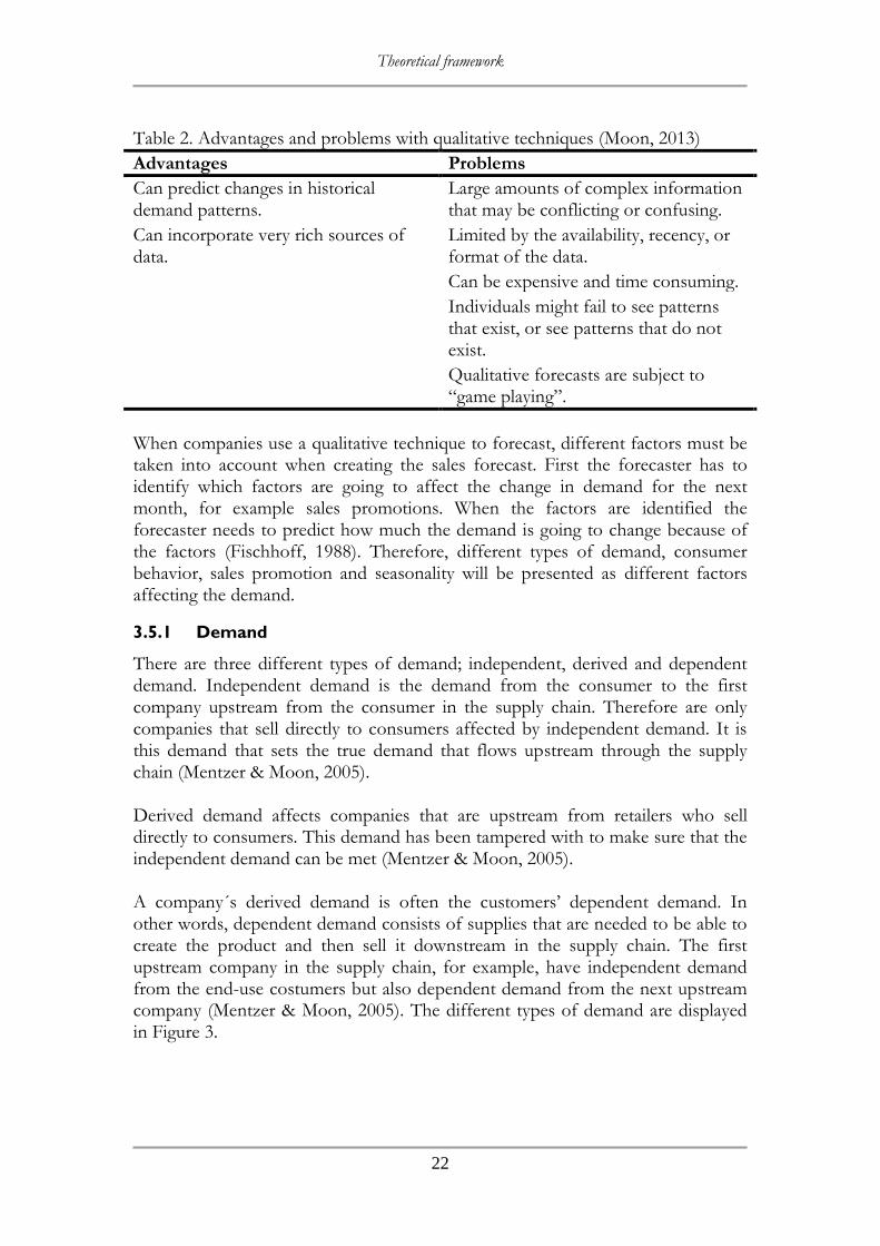
Moon (2013) defines qualitative forecasts as following: “qualitative forecasting (also called subjective or judgmental forecasting) is the process of capturing the opinions, knowledge, and intuition of experienced people, and turning those opinions, knowledge, and intuition into formal forecasts”. Qualitative techniques are the opposite to time series techniques, instead of looking at sales history, a qualitative approach tries to predict the future using only judgmental factors from experienced personnel (Mentzer & Moon, 2005; Moon, 2013). Even if a company uses time series techniques to forecast, there will always be qualitative techniques involved. The company has to decide which technique to use, what kind of data to collect, how to measure accuracy, evaluate the result, and so on, this requires a qualitative approach (Fischhoff, 1988; Mentzer & Moon, 2005; Moon, 2013; Yu, 2006). A qualitative approach is necessary when forecasting new products or a product without any historical data. In these cases experienced persons must try to predict the future by looking on, for example, similar products with historical data to get guidelines when forecasting. Moon (2013) mentions that there are more problems with qualitative forecasting than advantages, see Table 2, but qualitative techniques are a valuable resource for forecasters. A company should never disregard the value of experience and the ability to analyse complex situations as an input to sales forecast.
Theoretical framework
22
Table 2. Advantages and problems with qualitative techniques (Moon, 2013)
Advantages Problems
Can predict changes in historical demand patterns.
Large amounts of complex information that may be conflicting or confusing.
Can incorporate very rich sources of data.
Limited by the availability, recency, or format of the data.
Can be expensive and time consuming.
Individuals might fail to see patterns that exist, or see patterns that do not exist.
Qualitative forecasts are subject to “game playing”.
When companies use a qualitative technique to forecast, different factors must be taken into account when creating the sales forecast. First the forecaster has to identify which factors are going to affect the change in demand for the next month, for example sales promotions. When the factors are identified the forecaster needs to predict how much the demand is going to change because of the factors (Fischhoff, 1988). Therefore, different types of demand, consumer behavior, sales promotion and seasonality will be presented as different factors affecting the demand.
3.5.1 Demand
There are three different types of demand; independent, derived and dependent demand. Independent demand is the demand from the consumer to the first company upstream from the consumer in the supply chain. Therefore are only companies that sell directly to consumers affected by independent demand. It is this demand that sets the true demand that flows upstream through the supply chain (Mentzer & Moon, 2005). Derived demand affects companies that are upstream from retailers who sell directly to consumers. This demand has been tampered with to make sure that the independent demand can be met (Mentzer & Moon, 2005). A company´s derived demand is often the customers’ dependent demand. In other words, dependent demand consists of supplies that are needed to be able to create the product and then sell it downstream in the supply chain. The first upstream company in the supply chain, for example, have independent demand from the end-use costumers but also dependent demand from the next upstream company (Mentzer & Moon, 2005). The different types of demand are displayed in Figure 3.

Theoretical framework
23
Figure 3. Different types of demand
The techniques used for forecasting the different types of demand can vary and it is of importance to know how to deal with different types of demand. Mentzer and Moon (2005) suggests that independent demand is the only demand that is necessary to forecast as both dependent and derived demand can be planned rather than forecasted through better information flow within the supply chain.
3.5.2 Consumer behaviour
Consumer behaviour is another important factor to consider when sales forecasting. The behaviour of consumers is difficult to predict but with the right information more accurate predictions can be made (Currie & Rowley, 2010; Jonsson & Mattson, 2011). Consumers purchase different things, at different times through different networks so these predictions are therefore complicated since consumer behaviour constantly changes (Currie & Rowley, 2010). According to Foxall (2007) historical learning is a contributing factor to consumer buying behaviour. Historical learning means that consumers change the buying behaviour in regard to past experiences, both positive and negative. Additionally, historical learning also accounts for different personal factors that influence buyers in decisions, factors as ability to pay, consumers’ mood, impulses and deprivation. Currie and Rowley (2010) suggests that, because of historical learning, major disruptive events can change consumer behaviour and that permanently. It has been seen after credit crunches, the global financial crisis, and recessions, among others. The development of technology is an example that also has changed consumer behaviour drastically. Consumers have become smarter with the use of Internet; researching previous consumers’ reviews, or the use of comparison sites to seek out the best deals. As a result of these events Currie and Rowley (2010) further states that it has shown that consumer buying behaviour has changed significantly which leads to consumers becoming more strategic.
Theoretical framework
24
Because of these disruptive events, forecasts based on historical data have become less accurate. Historical data that has been gathered before a major event might not be usable after because of a permanent change in consumer buying behaviour because of historical learning (Currie & Rowley, 2010). These changes in consumer buying behaviour are important to understand to be able to make more accurate predictions of future demand. If understood it is also easier for companies to conduct more effective sales promotions and plan activities (Kotler, 2001).
3.5.3 Sales promotion
Sales promotion can be explained as something temporary a company does to attract customers to make quick purchases by for example reduced selling price, three-for-two sales, and free item along with purchased item. By reducing the price or increasing the benefits of the products the customer will receive a higher product value (Kotler et al., 2011). Sales promotion attempts from retailers are used for achieving uplifts in sales and these promotions should, to be more successful, be planned and used when forecasting sales of each product affected by the promotion. When planning promotion, information should be shared about, for instance, selling price, promotion during holidays or special occasions, or the length of the promotion period. Depending on the requirement of sales promotions when forecasting, the level of information sharing between the different companies in the supply chain can vary (Ramanathan, 2012). Ramanathan (2012) suggests that by collaborating with planning, forecasting and replenishment the performance of the sales promotion can be improved, as companies in the supply chain are prepared for an increase in demand and sales. This way the companies can minimize variation of demand, increase the forecast accuracy and avoid meeting the demand by using excessive inventory. The inventory can instead be kept to a minimum. Sales promotions should because of this, according to Ramanathan (2012), be considered as an important factor to take into account when forecasting sales.
3.5.4 Seasonality
Ramanathan (2012) further mentions seasonality as an important factor to consider when forecasting sales. Normally, demand for functional products as food and other consumables will have low demand-uncertainties, as sales tend not to change much over time. It is, however, different with innovative products, for example household appliances. Innovative products, though predictable in some extent, can be affected by seasonal factors like temperature, and holidays, among others. Depending on the type of information the company wants, complications when sales forecasting can arise. Seasonal information can be gathered in different ways depending on the kind of information. Information can be collected through publically available data, from sales history or collaboration within the supply chain (Ramanathan, 2012).
Theoretical framework
25
3.6 Time series
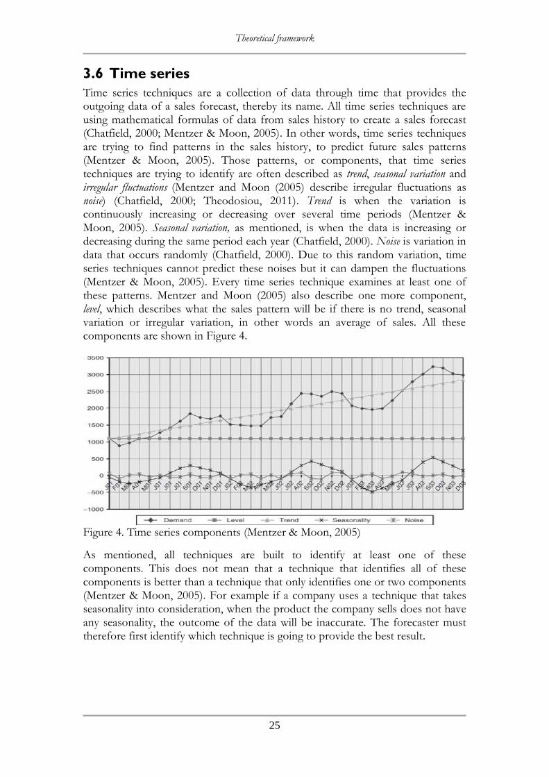
Time series techniques are a collection of data through time that provides the outgoing data of a sales forecast, thereby its name. All time series techniques are using mathematical formulas of data from sales history to create a sales forecast (Chatfield, 2000; Mentzer & Moon, 2005). In other words, time series techniques are trying to find patterns in the sales history, to predict future sales patterns (Mentzer & Moon, 2005). Those patterns, or components, that time series techniques are trying to identify are often described as trend, seasonal variation and irregular fluctuations (Mentzer and Moon (2005) describe irregular fluctuations as noise) (Chatfield, 2000; Theodosiou, 2011). Trend is when the variation is continuously increasing or decreasing over several time periods (Mentzer & Moon, 2005). Seasonal variation, as mentioned, is when the data is increasing or decreasing during the same period each year (Chatfield, 2000). Noise is variation in data that occurs randomly (Chatfield, 2000). Due to this random variation, time series techniques cannot predict these noises but it can dampen the fluctuations (Mentzer & Moon, 2005). Every time series technique examines at least one of these patterns. Mentzer and Moon (2005) also describe one more component, level, which describes what the sales pattern will be if there is no trend, seasonal variation or irregular variation, in other words an average of sales. All these components are shown in Figure 4.
Figure 4. Time series components (Mentzer & Moon, 2005)
As mentioned, all techniques are built to identify at least one of these components. This does not mean that a technique that identifies all of these components is better than a technique that only identifies one or two components (Mentzer & Moon, 2005). For example if a company uses a technique that takes seasonality into consideration, when the product the company sells does not have any seasonality, the outcome of the data will be inaccurate. The forecaster must therefore first identify which technique is going to provide the best result.
Theoretical framework
26
3.6.1 Exponential smoothing
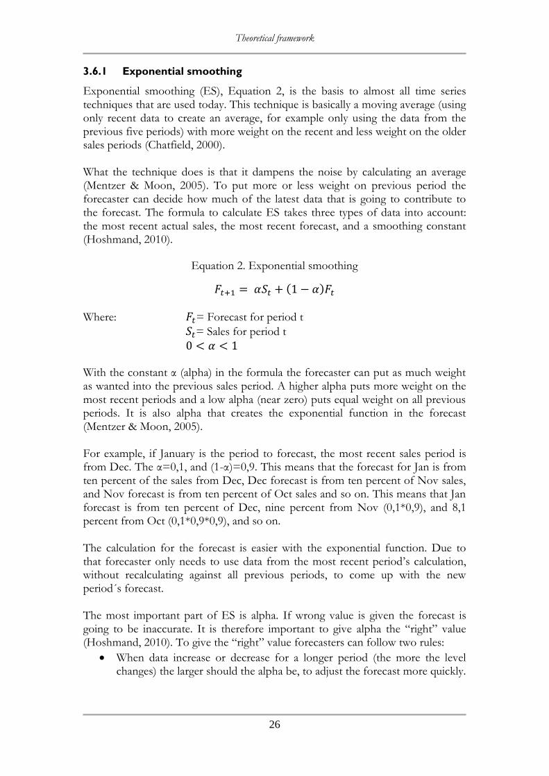
Exponential smoothing (ES), Equation 2, is the basis to almost all time series techniques that are used today. This technique is basically a moving average (using only recent data to create an average, for example only using the data from the previous five periods) with more weight on the recent and less weight on the older sales periods (Chatfield, 2000). What the technique does is that it dampens the noise by calculating an average (Mentzer & Moon, 2005). To put more or less weight on previous period the forecaster can decide how much of the latest data that is going to contribute to the forecast. The formula to calculate ES takes three types of data into account: the most recent actual sales, the most recent forecast, and a smoothing constant (Hoshmand, 2010).
Equation 2. Exponential smoothing
( )
Where: = Forecast for period t
= Sales for period t
With the constant α (alpha) in the formula the forecaster can put as much weight as wanted into the previous sales period. A higher alpha puts more weight on the most recent periods and a low alpha (near zero) puts equal weight on all previous periods. It is also alpha that creates the exponential function in the forecast (Mentzer & Moon, 2005). For example, if January is the period to forecast, the most recent sales period is from Dec. The α=0,1, and (1-α)=0,9. This means that the forecast for Jan is from ten percent of the sales from Dec, Dec forecast is from ten percent of Nov sales, and Nov forecast is from ten percent of Oct sales and so on. This means that Jan forecast is from ten percent of Dec, nine percent from Nov (0,1*0,9), and 8,1 percent from Oct (0,1*0,9*0,9), and so on. The calculation for the forecast is easier with the exponential function. Due to that forecaster only needs to use data from the most recent period’s calculation, without recalculating against all previous periods, to come up with the new period´s forecast. The most important part of ES is alpha. If wrong value is given the forecast is going to be inaccurate. It is therefore important to give alpha the “right” value (Hoshmand, 2010). To give the “right” value forecasters can follow two rules:
When data increase or decrease for a longer period (the more the level changes) the larger should the alpha be, to adjust the forecast more quickly.
Theoretical framework
27
When the data is random, alpha should be smaller so the noise is dampened (Hoshmand, 2010; Mentzer & Moon, 2005).
3.6.2 Exponential smoothing with trend
Trend is an important component to take into account for companies that want to forecast further into the future (for example the next 12 months) (Jonsson & Mattson, 2011). The exponential smoothing with trend (EST), Equation 5, provides this feature. The EST is basically the same as the original ES technique (it tries to dampen the noise by calculating an average) but it uses both trend and level (Mentzer & Moon, 2005). Due to the level and trend, the calculation will get one more constant, β (beta), this constant works in the same way as alpha (to put more weight into more recent periods). It is time consuming and costly to find the best combination between these two constants, the same two rules as in ES can therefore be used to reduce the cost and time to come up with the best combination (Hoshmand, 2010). An introduction of how trend and level are predicted is necessary to understand the formula that EST is using. To predict the level the following formula, Equation 3, is constructed:
Equation 3. Level
( )( ) Where: L = level T = trend
0<α<1
This calculation is similar to ES calculations but instead of using last period’s forecast it uses trend. The calculation for level is then needed to calculate the trend, Equation 4:
Equation 4. Trend
( ) ( ) Where: 0<β<1
( ) measures how much the level has changed from the two recent
periods and ( ) is the estimated trend from the last period. When both trend and level have been calculated the calculation for the forecast can be executed. This can be done by taking the new value of level and adding the new value of trend times the number of periods that are going to be forecasted (Mentzer & Moon, 2005).

Theoretical framework
28
Equation 5. Exponential smoothing with trend
( ) Where: m = the number of periods to forecast. To get a better understanding of the formula an example is presented:
Table 3. Example of calculation with exponential smoothing with trend
To make a sales forecast for May when the latest data is from January the formula gives the following calculation
( )
The tricky part of EST is not to calculate the forecast but to find the right combination between alpha and beta to get a more accurate forecast (Hoshmand, 2010; Mentzer & Moon, 2005).
3.6.3 Exponential smoothing with trend and seasonality
If a company has products that are seasonal, the forecasting technique exponential smoothing with trend and seasonality (ESTS), Equation 8, can be a way to forecast these products (Hoshmand, 2010). Mentzer and Moon (2005) mention, that ESTS can be seen as an extension to EST. Both techniques have to calculate level and trend before the actual forecast formula can be made. With ESTS, seasonal adjustment (SA), Equation 6, will also be calculated before the actual forecast formula can be made. SA is basically the difference between sales and level but with a smoothing constant γ (gamma) to put more weight on previous periods (Mentzer & Moon, 2005).
Equation 6. Seasonal adjustment
( ) ( )( )
Where: = Seasonal adjustment for period t C = Cycle length of the seasonal pattern (usually C = 12 (1 year)) 0<γ<1 There is also a difference in the calculation for level compared to EST. Instead of multiplying the smoothing constant with sales, alpha is multiplied with sales divided with last year period´s SA. When dividing sales with last year’s SA the
Month Sales Level Trend Forecast
Jan 4000 3996 121 3996
Theoretical framework
29
seasonality for that specific period is taken out, see Equation 7 (Mentzer & Moon, 2005).
Equation 7. Level with seasonal adjustment
(
) ( )( )
Where: 0<α<1 The calculation of trend is the same as in the previous technique, EST. After the new estimated values of level, trend, and seasonality, the forecast can be calculated by taken the level added with trend times the period that is going to be forecasted, and multiplying the result with the most recent SA for that specific period (Mentzer & Moon, 2005).
Equation 8. Exponential smoothing with trend and seasonality
( ( ))
The main problem with this technique is that it needs data from at least one year back in time before the forecast can give valuable information about future demand (Hoshmand, 2010). It is also an issue to select the proper combination between the smoothing constants. The accuracy of the forecast is depending on the right combination between the constants (Mentzer & Moon, 2005).


Empirical data
31
4 Empirical data
In this chapter, the empirical data collected through the case study will be presented. Information about the case company is followed by the case company’s current forecasting process. The chapter will end with a presentation about the case company´s current measurement of accuracy.
4.1 Case company
The case study was performed at Electrolux AB Thailand, part of Electrolux AB, who manufactures and sells household appliances. Electrolux AB´s operations are spread over four different areas, which can be seen in Figure 5 with Thailand being part of Southeast Asia in the Asian/Pacific region (Electrolux AB, 2014). Electrolux AB was founded in Sweden 1919 and is now selling 50 million products to customers in 150 countries each year with North America and Europe being the largest markets. Electrolux AB is, with its 61 000 employees and an annual revenue of 16,7 billion dollar, a global leader within the industry of household appliances. Electrolux AB has offices spread out in different countries in the world and is since 1977 also operating an office in Thailand, selling household appliances both through own stores and retailers. Because of the increasing demand in Southeast Asia a new factory for manufacturing refrigerators opened in Rayong, Thailand in 2013. It not only serves the purpose of supplying the increasing demand in Southeast Asia but also leads the company’s refrigerator manufacturing for the global market (Electrolux AB, 2014).
Figure 5. Electrolux AB´s organisational structure
In the case study, Electrolux AB’s forecasting process was evaluated to find areas for improvement and to try to increase the accuracy of the company’s sales
Electrolux Group
North America Latin America Asia/Pacific
Australia & New Zeeland
Southeast Asia
Malaysia Philipines Thailand Singapore Vietnam
China, Taiwan, Korea, Japan
Europe/Middle east/Africa
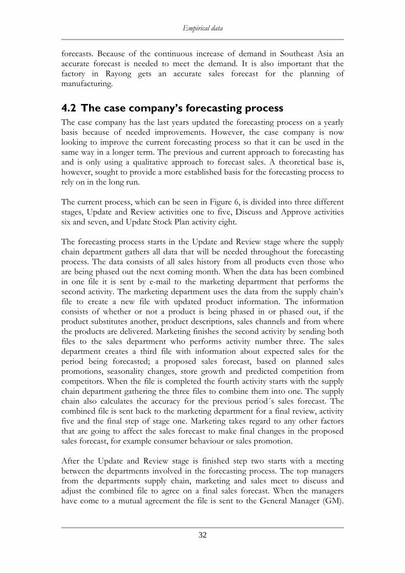
Empirical data
32
forecasts. Because of the continuous increase of demand in Southeast Asia an accurate forecast is needed to meet the demand. It is also important that the factory in Rayong gets an accurate sales forecast for the planning of manufacturing.
4.2 The case company’s forecasting process
The case company has the last years updated the forecasting process on a yearly basis because of needed improvements. However, the case company is now looking to improve the current forecasting process so that it can be used in the same way in a longer term. The previous and current approach to forecasting has and is only using a qualitative approach to forecast sales. A theoretical base is, however, sought to provide a more established basis for the forecasting process to rely on in the long run. The current process, which can be seen in Figure 6, is divided into three different stages, Update and Review activities one to five, Discuss and Approve activities six and seven, and Update Stock Plan activity eight. The forecasting process starts in the Update and Review stage where the supply chain department gathers all data that will be needed throughout the forecasting process. The data consists of all sales history from all products even those who are being phased out the next coming month. When the data has been combined in one file it is sent by e-mail to the marketing department that performs the second activity. The marketing department uses the data from the supply chain’s file to create a new file with updated product information. The information consists of whether or not a product is being phased in or phased out, if the product substitutes another, product descriptions, sales channels and from where the products are delivered. Marketing finishes the second activity by sending both files to the sales department who performs activity number three. The sales department creates a third file with information about expected sales for the period being forecasted; a proposed sales forecast, based on planned sales promotions, seasonality changes, store growth and predicted competition from competitors. When the file is completed the fourth activity starts with the supply chain department gathering the three files to combine them into one. The supply chain also calculates the accuracy for the previous period´s sales forecast. The combined file is sent back to the marketing department for a final review, activity five and the final step of stage one. Marketing takes regard to any other factors that are going to affect the sales forecast to make final changes in the proposed sales forecast, for example consumer behaviour or sales promotion. After the Update and Review stage is finished step two starts with a meeting between the departments involved in the forecasting process. The top managers from the departments supply chain, marketing and sales meet to discuss and adjust the combined file to agree on a final sales forecast. When the managers have come to a mutual agreement the file is sent to the General Manager (GM).
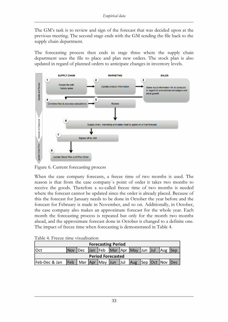
Empirical data
33
The GM’s task is to review and sign of the forecast that was decided upon at the previous meeting. The second stage ends with the GM sending the file back to the supply chain department. The forecasting process then ends in stage three where the supply chain department uses the file to place and plan new orders. The stock plan is also updated in regard of planned orders to anticipate changes in inventory levels.
Figure 6. Current forecasting process
When the case company forecasts, a freeze time of two months is used. The reason is that from the case company´s point of order it takes two months to receive the goods. Therefore a so-called freeze time of two months is needed where the forecast cannot be updated since the order is already placed. Because of this the forecast for January needs to be done in October the year before and the forecast for February is made in November, and so on. Additionally, in October, the case company also makes an approximate forecast for the whole year. Each month the forecasting process is repeated but only for the month two months ahead, and the approximate forecast done in October is changed to a definite one. The impact of freeze time when forecasting is demonstrated in Table 4. Table 4. Freeze time visualisation
Oct Nov Dec Jan Feb Mar Apr May Jun Jul Aug Sep
Feb-Dec & Jan Feb Mar Apr May Jun Jul Aug Sep Oct Nov Dec
Forecasting Period
Period Forecasted
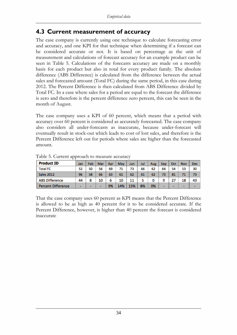
Empirical data
34
4.3 Current measurement of accuracy
The case company is currently using one technique to calculate forecasting error and accuracy, and one KPI for that technique when determining if a forecast can be considered accurate or not. It is based on percentage as the unit of measurement and calculations of forecast accuracy for an example product can be seen in Table 5. Calculations of the forecasts accuracy are made on a monthly basis for each product but also in total for every product family. The absolute difference (ABS Difference) is calculated from the difference between the actual sales and forecasted amount (Total FC) during the same period, in this case during 2012. The Percent Difference is then calculated from ABS Difference divided by Total FC. In a case where sales for a period are equal to the forecast the difference is zero and therefore is the percent difference zero percent, this can be seen in the month of August. The case company uses a KPI of 60 percent, which means that a period with accuracy over 60 percent is considered as accurately forecasted. The case company also considers all under-forecasts as inaccurate, because under-forecast will eventually result in stock-out which leads to cost of lost sales, and therefore is the Percent Difference left out for periods where sales are higher than the forecasted amount. Table 5. Current approach to measure accuracy
That the case company uses 60 percent as KPI means that the Percent Difference is allowed to be as high as 40 percent for it to be considered accurate. If the Percent Difference, however, is higher than 40 percent the forecast is considered inaccurate
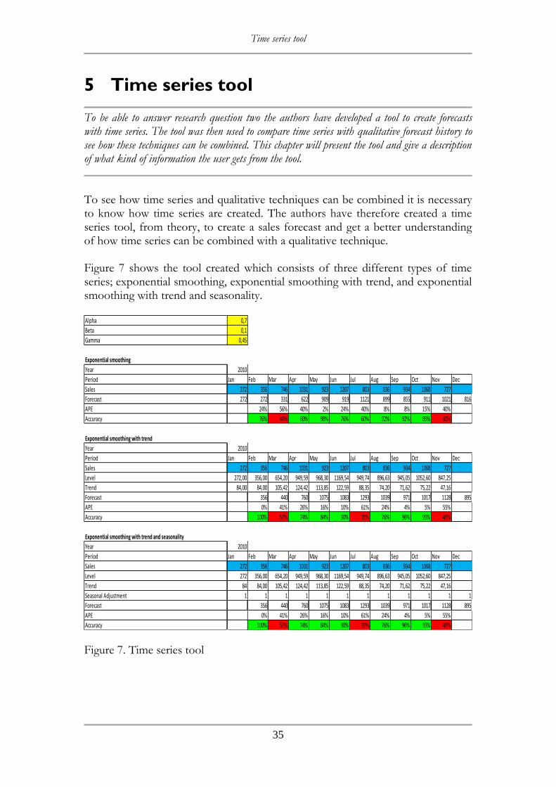
Time series tool
35
5 Time series tool
To be able to answer research question two the authors have developed a tool to create forecasts with time series. The tool was then used to compare time series with qualitative forecast history to see how these techniques can be combined. This chapter will present the tool and give a description of what kind of information the user gets from the tool.
To see how time series and qualitative techniques can be combined it is necessary to know how time series are created. The authors have therefore created a time series tool, from theory, to create a sales forecast and get a better understanding of how time series can be combined with a qualitative technique. Figure 7 shows the tool created which consists of three different types of time series; exponential smoothing, exponential smoothing with trend, and exponential smoothing with trend and seasonality.
Figure 7. Time series tool
Alpha 0,7
Beta 0,1
Gamma 0,45
Exponential smoothing
Year 2010
Period Jan Feb Mar Apr May Jun Jul Aug Sep Oct Nov Dec
Sales 272 356 746 1031 923 1207 803 836 934 1068 727
Forecast 272 272 331 622 909 919 1121 899 855 911 1021 816
APE 24% 56% 40% 2% 24% 40% 8% 8% 15% 40%
Accuracy 76% 44% 60% 98% 76% 60% 92% 92% 85% 60%
Exponential smoothing with trend
Year 2010
Period Jan Feb Mar Apr May Jun Jul Aug Sep Oct Nov Dec
Sales 272 356 746 1031 923 1207 803 836 934 1068 727
Level 272,00 356,00 654,20 949,59 968,30 1169,54 949,74 896,63 945,05 1052,60 847,25
Trend 84,00 84,00 105,42 124,42 113,85 122,59 88,35 74,20 71,62 75,22 47,16
Forecast 356 440 760 1075 1083 1293 1039 971 1017 1128 895
APE 0% 41% 26% 16% 10% 61% 24% 4% 5% 55%
Accuracy 100% 59% 74% 84% 90% 39% 76% 96% 95% 45%
Exponential smoothing with trend and seasonality
Year 2010
Period Jan Feb Mar Apr May Jun Jul Aug Sep Oct Nov Dec
Sales 272 356 746 1031 923 1207 803 836 934 1068 727
Level 272 356,00 654,20 949,59 968,30 1169,54 949,74 896,63 945,05 1052,60 847,25
Trend 84 84,00 105,42 124,42 113,85 122,59 88,35 74,20 71,62 75,22 47,16
Seasonal Adjustment 1 1 1 1 1 1 1 1 1 1 1 1
Forecast 356 440 760 1075 1083 1293 1039 971 1017 1128 895
APE 0% 41% 26% 16% 10% 61% 24% 4% 5% 55%
Accuracy 100% 59% 74% 84% 90% 39% 76% 96% 95% 45%
Time series tool
36
This tool is created in a way that makes it easy to understand and decreases the workload when forecasting. The main information the user gets from the tool is what the forecast is for the next period (Forecast), how much the forecast error was from previous periods (APE), and if the previous forecasted periods have reached the KPI (Accuracy). The user needs to put sales history from the previous periods´ actual sales into the blue squares; the tool does the rest of the calculations (except for the first period). The user also needs to calculate the values on the constants that are used and enter it into the yellow squares. Once the constants are calculated for one specific product the constants do not need to be changed. In other words the user only needs to put in new values on the constants when forecasting products that are new to the tool. As mentioned, the tool cannot generate a forecast for the first period automatically, the user must therefore put in level, trend, seasonal adjustment, and forecast manually for the first period. To do so there are some rules; the level is equal the first period of sales, trend is equal the next period of sales minus the current period of sales, seasonal adjustment is equal to one the whole first forecasted year, and the forecast for the first period is equal to the forecast made by a qualitative technique.
Exponential smoothing
The information the tool provides with exponential smoothing is what year it is, which period the forecast is for, the actual sales for the period, the forecast for the same period, the forecast error, and the accuracy for the same period. This technique is the easiest to create but it cannot make a forecast for more than one period ahead.
Exponential smoothing with trend
The tool provides the same information as for exponential smoothing but with two additional factors: level and trend. The level displays how much the weighted average sales would have been if there would be no trend (and seasonal adjustment in the next technique). The trend gives information regarding if the demand is increasing or decreasing. If the trend has a negative value for a longer time, the demand is decreasing and if the trend has a positive value the demand is increasing. In a case where the trend has both negative and positive values for a longer time the demand then have irregular fluctuations.
Exponential smoothing with trend and seasonality
The tool provides one additional factor with exponential smoothing with trend and seasonality; seasonal adjustment. Seasonal adjustment gives information whether or not a product is affected by seasonality. If the seasonal adjustment constantly increases or decreases during a specific period every year, it means that the product has seasonality. But if the seasonal adjustment does not increase or decrease for one specific period each year, or if it is just a change for one year and not the other, it means that the product does not have any seasonality.
Time series tool
37
Disadvantages
The main disadvantage with the tool is that the user needs to find the best combination between the constants without any pre-installed calculations. It is this combination that either increases or decreases the forecast´s accuracy. This is therefore the main focus when it comes to improvements of the tool. Other disadvantages are that the technique ES cannot make a forecast more than one period into the future; this is because the formula for this technique does not provide it. Fortunately both EST and ESTS can forecast as far into the future as the user wants by a little change in the forecast formula, this is described in chapter 3.6.2 and 3.6.3. The user must, however, be aware that ESTS needs more than one year of history before it can create an accurate forecast. The seasonal adjustment is 1,00 through the whole year, this factor will not be adjusted until after at least one year, and not until then should this technique be used.
Advantages
The greatest advantages with the tool, if disregarding the problem with the constants, is the time saved by forecasting with the tool, by only typing in sales history from the previous period. For example if the user wants to make a forecast for February 2014, all that is needed is to insert the actual sales from January. The tool also displays, by turning the accuracy either green or red, if the forecast for each month can be consider accurate. With this function the user can easily see if the forecast needs to be improved or not. Another advantage is that the KPI for measuring the accuracy can be changed easily; this makes the tool useable, not only for the case company, but also for other companies with similar situations. If the user wants to measure the accuracy in another way than APE the user needs to add a new row with the desired formula for calculating accuracy. In other words, the tool has a high grade of adaptability due to that it is easy to add or remove factors in the tool.

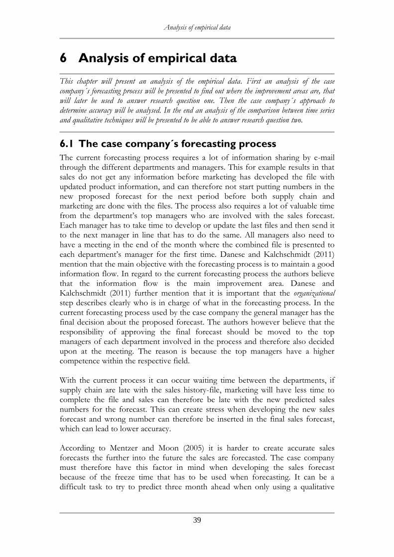
Analysis of empirical data
39
6 Analysis of empirical data
This chapter will present an analysis of the empirical data. First an analysis of the case company´s forecasting process will be presented to find out where the improvement areas are, that will later be used to answer research question one. Then the case company´s approach to determine accuracy will be analysed. In the end an analysis of the comparison between time series and qualitative techniques will be presented to be able to answer research question two.
6.1 The case company´s forecasting process
The current forecasting process requires a lot of information sharing by e-mail through the different departments and managers. This for example results in that sales do not get any information before marketing has developed the file with updated product information, and can therefore not start putting numbers in the new proposed forecast for the next period before both supply chain and marketing are done with the files. The process also requires a lot of valuable time from the department’s top managers who are involved with the sales forecast. Each manager has to take time to develop or update the last files and then send it to the next manager in line that has to do the same. All managers also need to have a meeting in the end of the month where the combined file is presented to each department’s manager for the first time. Danese and Kalchschmidt (2011) mention that the main objective with the forecasting process is to maintain a good information flow. In regard to the current forecasting process the authors believe that the information flow is the main improvement area. Danese and Kalchschmidt (2011) further mention that it is important that the organizational step describes clearly who is in charge of what in the forecasting process. In the current forecasting process used by the case company the general manager has the final decision about the proposed forecast. The authors however believe that the responsibility of approving the final forecast should be moved to the top managers of each department involved in the process and therefore also decided upon at the meeting. The reason is because the top managers have a higher competence within the respective field. With the current process it can occur waiting time between the departments, if supply chain are late with the sales history-file, marketing will have less time to complete the file and sales can therefore be late with the new predicted sales numbers for the forecast. This can create stress when developing the new sales forecast and wrong number can therefore be inserted in the final sales forecast, which can lead to lower accuracy. According to Mentzer and Moon (2005) it is harder to create accurate sales forecasts the further into the future the sales are forecasted. The case company must therefore have this factor in mind when developing the sales forecast because of the freeze time that has to be used when forecasting. It can be a difficult task to try to predict three month ahead when only using a qualitative

Analysis of empirical data
40
technique. The authors will therefore in chapter 6.3 analyse if time series can provide more accurate forecasts. This is also seen as an improvement area for the first step in the forecasting process, information-gathering and tools that Danese and Kalchschmidt (2011) refers to, as a time series tool provides additional information as a foundation to the proposed forecast.
6.2 Current measurement of accuracy
The case company is currently using one technique, ABS Difference, and a KPI of 60 percent to determine whether the sales forecast can be considered as accurate or not. Further, the case company also considers all under-forecasts as inaccurate, as under-forecasts eventually will result in a stock-out and should therefore not be considered as accurate. In case of an under-forecast the accuracy of the under-forecast is not taken into account. A consequence of using ABS Difference and not take under-forecasts into account is that it makes it harder to receive data from inaccurate forecasts. For example it can complicate the calculation of the total under-forecast of a certain period to determine how much more stock would have been needed to supply the demand. The case company also uses the same KPI for all products and product groups instead of determining a KPI for each product or product group based on the products value and number of units, as is suggested by Mentzer and Moon (2005). This could impact the company negatively as products with higher value will affect the company more than low value products if forecasted inaccurately. Calculations of forecast accuracy is also only made on a monthly basis and not summarized for each quarter or year to further calculate the mean accuracy during the same period. The technique used will only provide difference and accuracy for each period but as under-forecasts are not taken into account, calculations of how the forecast has performed over a number of periods cannot be calculated.
6.3 Time series compared to qualitative sales forecast
As mentioned earlier the case company is only using a qualitative technique to create the sales forecast. This means that every time the case company creates new sales forecasts, important labour hours from top manager are needed to be able to create the sales forecast. This chapter will present the results from the comparison of the forecast from the tool and the case company´s forecast to identify if time and cost can be saved by using time series.
6.3.1 Exponential smoothing
The upper forecast in Table 6 is the case company´s and the lower is the time series tool. The tool uses ES, because the sales history only contains sales from one year and ESTS needs more than one year to be able to perform accurate forecasts. The reason for not choosing EST was because the sales were relatively constant and therefore is ES better to use. By calculating the APE for each month and each forecast the authors could compare the sales forecasts created to see
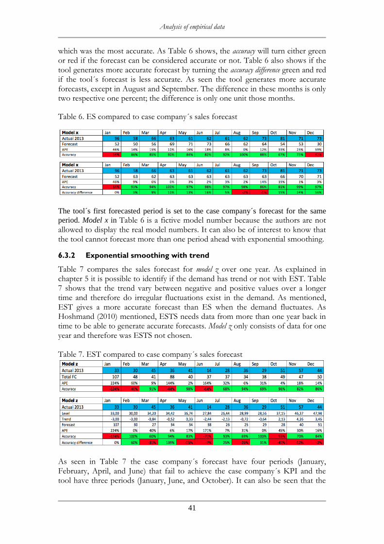
Analysis of empirical data
41
which was the most accurate. As Table 6 shows, the accuracy will turn either green or red if the forecast can be considered accurate or not. Table 6 also shows if the tool generates more accurate forecast by turning the accuracy difference green and red if the tool´s forecast is less accurate. As seen the tool generates more accurate forecasts, except in August and September. The difference in these months is only two respective one percent; the difference is only one unit those months.
Table 6. ES compared to case company´s sales forecast
The tool´s first forecasted period is set to the case company´s forecast for the same
period. Model x in Table 6 is a fictive model number because the authors are not allowed to display the real model numbers. It can also be of interest to know that the tool cannot forecast more than one period ahead with exponential smoothing.
6.3.2 Exponential smoothing with trend
Table 7 compares the sales forecast for model z over one year. As explained in chapter 5 it is possible to identify if the demand has trend or not with EST. Table 7 shows that the trend vary between negative and positive values over a longer time and therefore do irregular fluctuations exist in the demand. As mentioned, EST gives a more accurate forecast than ES when the demand fluctuates. As Hoshmand (2010) mentioned, ESTS needs data from more than one year back in time to be able to generate accurate forecasts. Model z only consists of data for one year and therefore was ESTS not chosen. Table 7. EST compared to case company´s sales forecast
As seen in Table 7 the case company´s forecast have four periods (January, February, April, and June) that fail to achieve the case company´s KPI and the tool have three periods (January, June, and October). It can also be seen that the

Analysis of empirical data
42
tool have more periods that are less accurate then the case company´s forecast (Mars, May, June, August, October, November, and December), this does however not mean that the tool is less accurate than the case company´s forecast. When it is hard to identify, with own eyes, which forecast is more accurate a good approach can be to calculate the average of the forecasting error; MAPE. MAPE
for the case company´s forecast would be
and
the tool would get
. This means that the case
company´s forecast have an average of 59 percent forecasting error each month, which will give an average accuracy of 41 percent each month. The tool has an average of 49 percent forecasting error, which gives an average of 51 percent accuracy each month. This average is for the year that Table 7 displays; the sum of the forecasting error is therefore divided by twelve. As it shows the tool will provide a more accurate average then the case company´s forecast but none of the forecasts average of the accuracy is able to achieve the KPI.
6.3.3 Exponential smoothing with trend and seasonality
Model y, as can be seen in Appendix 3, have sales history from January 2011 to April 2014. As mentioned ESTS need sales history from at least a year back in time and therefore can ESTS be used to model y. When forecasting products for several years and all seasonal patterns have been identified the time series tool can be used to make accurate sales forecasts. As Table 8 shows, the forecast from the tool generates a more accurate value for each period than what the case company´s forecast does. But the beginning of the tool’s forecast is not as accurate as the case company´s, as can be seen in Appendix 3. This will later be discussed in chapter 8.
Table 8. ESTS compared to case company´s sales forecast
By looking at Table 8 it can be seen that seasonal adjustment for each period is relatively constant, the only month when the seasonal adjustment varies is in April (1, 0.95, 0.95, and 0.96) the other months SA is around 1,00. The model y therefore has a little negative seasonality in April (the demand is lower than usual). Table 8 also shows that trend has negative values the first 16 periods and positive values
Feb Mar Apr May Jun Jul Aug Sep Oct Nov Dec Jan Feb Mar Apr
60 84 96 108 80 92 91 97 53 94 66 113 108 161 116
102 115 106 107 117 111 94 93 100 97 98 141 141 170 161
70% 37% 10% 1% 46% 21% 3% 4% 89% 3% 48% 25% 31% 6% 39%
30% 63% 90% 99% 54% 79% 97% 96% 11% 97% 52% 75% 69% 94% 61%
Feb Mar Apr May Jun Jul Aug Sep Oct Nov Dec Jan Feb Mar Apr
60 84 96 108 80 92 91 97 53 94 66 113 108 161 116
79 80 86 91 90 92 92 95 85 87 82 89 94 110 115
1 1 1 2 1 2 1 2 0 0 -1 1 1 3 4
1,013796 1,033178 0,959351 1,059824 0,998217 0,99251 1,020217 0,989998 0,992049 1,00156 0,982675 1,033289 1,020656 1,054562 0,961611
91 87 86 86 83 90 100 94 98 97 99 87 90 84 87
52% 4% 10% 20% 4% 2% 10% 3% 85% 3% 50% 23% 17% 48% 25%
48% 96% 90% 80% 96% 98% 90% 97% 15% 97% 50% 77% 83% 52% 75%
18% 33% 0% -19% 43% 18% -7% 1% 4% 0% -2% 2% 14% -42% 14%

Analysis of empirical data
43
the remaining periods. It can also be seen that the negative value has its lowest point after period five and continuously increase after period five. This means that model y has a positive trend with an increasing demand.
6.3.4 Sales forecast with time series
It can be identified that time series provide more accurate sales forecasts than qualitative techniques. The ES technique created more accurate sales forecast than EST and ESTS, however, the case company cannot use this technique because of the freeze time. The authors have been comparing more than the models above to see if the tool can be trustworthy. In eight of ten cases, the tool did provide a more accurate forecast. It was only when the sales were fluctuating a lot that the tool did not provide a more accurate forecast, but overall the time series tool gave a more accurate sales forecast. The case company could therefore improve the accuracy by only using time series as a forecasting technique. This should, however, not be done due to the deficiencies time series can have, which will be discussed in chapter 8.

Recommended approach to forecasting
45
7 Recommended approach to forecasting
This chapter will present the authors recommendations to the case company´s current situation. The chapter starts with a recommended approach to the forecasting process that now includes time series and qualitative techniques. In the end, two recommended approaches on how to determine the sales forecast accuracy will be presented.
7.1 Forecasting process
The authors have created a new process, which can be seen in Figure 8, that facilitates the information flow, and can be followed when forecasting and hopefully save valuable time for the top managers. As mentioned, the current process requires a lot of information sharing through e-mail. To facilitate the information flow among the departments the process now includes a database used to compile all the information, as suggested by Moon et al. (2013). The different departments can enter own data into the database for later consolidation and review. The different departments can this way enter the data simultaneously. However, when revising with the case company they had requests on deadlines that still need to be met by the different departments when it comes to putting in data. This is because some of the steps that a department needs to do can only be done once all steps from the previous department are completed. For example, supply chain can only finish the upload of history of sales once marketing have updated all products. It is however possible to start uploading history of sales as soon as marketing is done with a specific product or product group. That is why the marketing department has the deadline before supply chain. The reason for the change of the departments order in the process compared to the current process is because it is an unnecessary workload for supply chain to upload history of sales for products that ultimately will be phased out or discontinued. Therefore the marketing department needs to finish the task ahead of the supply chain department. Marketing still updates the general product information, which includes adding new models, deleting models that are discontinued or describing whether or not products substitutes another products. Supply chain uploads sales history for the previous month about the products that marketing updated to support predictions about the future. Supply chain also creates a proposed sales forecast with time series calculations for the upcoming forecast period and accuracy calculations for previous month. Sales create a proposed sales forecast for those models that time series cannot be used for. The data is stored in the database until supply chain obtains the information from the database in one combined Microsoft Excel-file and then shares it through the database. This will enable each top manager to have the ability to review the data as it is being put into the database by other departments. It further allows the managers to review the proposed sales forecasts in the database before the actual meeting.

Recommended approach to forecasting
46
A meeting is held where top manager from each department meets to discuss the data in the file to come up with a mutual and shared view of the sales forecast. When a consolidated sales forecast has been made it is used for updating the order plan. The activity where the GM signs of the sales forecast is gone because the authors believes the predetermined forecasting roles will ensure that right data is used when forecasting and the GM does therefore not need to review it. The forecasting process is constantly on-going with updates being made in the database and the first week of each month the process ends with a meeting to start all-over again with marketing updating the product information.
Figure 8. Recommended forecasting process
As Moon et al. (2003) suggested that with a shared database, where all departments can take and put in new information about the sales forecast, the company can achieve better information flow among the employees in different departments and therefore ensure that right data is used when forecasting.
7.2 Accuracy measurements
The authors have presented two alternative techniques for determining the sales forecast accuracy.
7.2.1 Percent error as measurement
The first technique is using PE to calculate forecasting error and then using the PE to calculate the accuracy of the forecast. If the PE is added with one, the sum is how accurate the forecast can be considered. A forecast with zero percent error is therefore 100 percent accurate, which can be seen in the month of August in Table 9. This way when the case company uses PE to determine if the forecast is accurate, with the same KPI of 60 percent, an interval of 60-140 percent should be used. The reason for an interval instead of the single value of 60 percent is that the value from this kind of calculation, that does not use absolute values, can get above 100 percent. In case of an under-forecast the considered accuracy will be
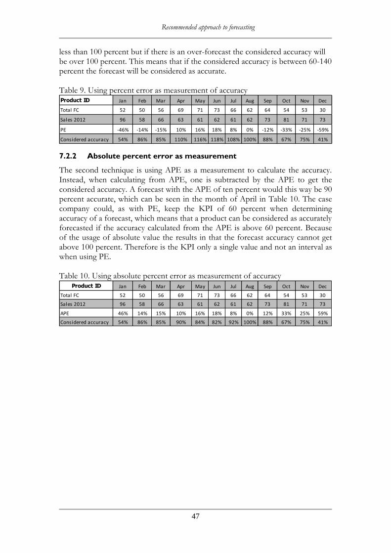
Recommended approach to forecasting
47
less than 100 percent but if there is an over-forecast the considered accuracy will be over 100 percent. This means that if the considered accuracy is between 60-140 percent the forecast will be considered as accurate. Table 9. Using percent error as measurement of accuracy
7.2.2 Absolute percent error as measurement
The second technique is using APE as a measurement to calculate the accuracy. Instead, when calculating from APE, one is subtracted by the APE to get the considered accuracy. A forecast with the APE of ten percent would this way be 90 percent accurate, which can be seen in the month of April in Table 10. The case company could, as with PE, keep the KPI of 60 percent when determining accuracy of a forecast, which means that a product can be considered as accurately forecasted if the accuracy calculated from the APE is above 60 percent. Because of the usage of absolute value the results in that the forecast accuracy cannot get above 100 percent. Therefore is the KPI only a single value and not an interval as when using PE. Table 10. Using absolute percent error as measurement of accuracy
Product ID Jan Feb Mar Apr May Jun Jul Aug Sep Oct Nov Dec
Total FC 52 50 56 69 71 73 66 62 64 54 53 30
Sales 2012 96 58 66 63 61 62 61 62 73 81 71 73
PE -46% -14% -15% 10% 16% 18% 8% 0% -12% -33% -25% -59%
Considered accuracy 54% 86% 85% 110% 116% 118% 108% 100% 88% 67% 75% 41%
Product ID Jan Feb Mar Apr May Jun Jul Aug Sep Oct Nov Dec
Total FC 52 50 56 69 71 73 66 62 64 54 53 30
Sales 2012 96 58 66 63 61 62 61 62 73 81 71 73
APE 46% 14% 15% 10% 16% 18% 8% 0% 12% 33% 25% 59%
Considered accuracy 54% 86% 85% 90% 84% 82% 92% 100% 88% 67% 75% 41%

Discussion and conclusion
49
8 Discussion and conclusion
This chapter presents a discussion of the result of the thesis work. The result discussion is divided into the research questions to make it easy for the reader to see the answer for each research question. There is also a methodology discussion where the authors evaluate the way the thesis work was conducted. The chapter ends with conclusions and areas for future studies within the subject.
8.1 Result
The purpose of the thesis was to investigate how to increase sales forecast accuracy. To fulfil the purpose the authors formed two research questions to answer. The discussion of the result will follow these two research questions that are answered separately.
8.1.1 What should be considered when developing a forecasting
process?
Danese and Kalchschmidt (2011) mentioned that a forecasting process can be divided into four steps, research question one´s answer will be based on these steps.
Information-gathering and tools
The first step in a forecasting process is to gather information regarding the sales forecast so that a forecast can be created. The information that needs to be collected is depending on what forecasting technique a company uses, for example if a company is relying on time series they must gather information about sales history. It is also important to know what is going to affect the demand when sales forecasting, if a company plan to do promotional activities, such as price changes, information about this must be collected before creating a sales forecast, otherwise the sales forecast can become inaccurate. It is therefore important that companies take time to analyse what kind of information is needed to be collected to create an accurate sales forecast. How the information should be collected is up to each company to decide. The authors, however, agree with Moon et al. (2003) that having a shared database (as in the proposed forecasting process) is a good way to collect and share information. With a shared database all departments within the company have access to all information within the company. However, the information that is put into the database must be sorted and simplified so others can understand and use the information. To sort up the collected data Microsoft Excel can be a good tool to use because it is easy to use and understand. Once the collected data is sorted and simplified in Microsoft Excel it can be put into the database and shared with all other departments. The authors do believe that this step is the most important one because it decides what kind of information and how the information is going to be flowing within
Discussion and conclusion
50
the company. If a company uses wrong information when forecasting the forecast is going to be inaccurate. It is therefore important that right information is used and shared in a good way, otherwise the forecast will become inaccurate even if the other steps are performed in a proper way.
Organizational
Danese and Kalchschmidt (2011) mention that the main objective with a forecasting process is to maintain good information flow. With good information flow the right information will be shared to the right source in the right time. To be able to achieve this, predetermined forecasting roles need to be assigned to each employee/department (source) so everyone within the company knows who is in charge of which part in the forecasting process. With clear predetermined forecasting roles the company ensures that the information will reach the right source. If the company sets up deadlines for each source, when the information needs to be ready, the company can ensure that the information will be on time to the next source (e.g. the deadline in the recommended forecasting process). If companies have predetermined forecasting roles, expertise will be created in each role and it will therefore be easier to ensure that the right information is gathered. When selecting the predetermined roles it is important to select a proper source to each step in the forecasting process, for example the production department should not create a proposed sales forecast because they do not have as much knowledge about the market as the marketing or the sales department have. It is therefore important for companies to carefully select the predetermined roles so the right competence is in the right place. This will ensure that the data used to forecast is as accurate as possible and will therefore, according to Lawrence et al. (2000), generate more accurate outgoing data (the forecast). By looking at Figure 8 it can be seen how a company can delegate different predetermined forecasting roles to ensure that the information is accurate and shared to the right source in the right time.
Interfunctional and intercompany
Depending on which departments are involved in the forecasting process the departments provide different kinds of information. At the case company the departments involved in the forecasting process are: supply chain, marketing and sales. As mentioned in the organizational step it is important that each department is aware of what information they will contribute with to the forecast. For example the sales department provides information about sales channels and store growth because that is what they know best while marketing provides information about sales promotion activities and other market-related factors that can affect the demand. In the proposed process supply chain do not just upload sales history but also provides the forecast accuracy for the previous period and time series calculations for the next period. According to Gilmore and Lewis (2006), the forecast accuracy will increase when departments work together and provide different kinds of information to create the forecast. It is however important to
Discussion and conclusion
51
keep in mind that the forecasting process becomes more complicated as more information is regarded. Mentzer and Moon (2005) further states that improved information flow, not only within the company but the supply chain as whole, improves the forecast accuracy. This is mainly because Mentzer and Moon (2005) suggests that dependant and derived demand can be planned rather than forecasted. The authors therefore believe that the case company could improve the forecast with better communication within the supply chain. For example the case company only needs to forecast products that the retailers sell, which is the independent demand. With better information flow the case company can collect this information more easily.
Measurement of accuracy
The fourth step in the forecasting process is the measurement of accuracy, if the right technique is used to measure accuracy (Danese & Kalchschmidt, 2011). As mentioned in chapter 4.3 the case company uses ABS Difference in percent as measurement of accuracy and thereafter a KPI to determine the performance of the forecast. The case company also do not take under-forecasts into account, which the authors believe is wrong. The authors therefore proposed two alternative ways to measure accuracy, PE and APE, which would provide the case company with additional data about the forecasts performance. Choosing the measurement for accuracy was however not the most difficult part. The authors found that the difficult part is to put the results from the measurements in regard of expected results, otherwise the performance cannot be judged. In other words, it is complicated to determine the right KPI to compare the result against and to measure the performance. To determine the KPI the company needs to consider the same factors that in any way can affect the performance of the forecast, the same factors that affect the demand, as the KPI is the expected performance of the forecast. It requires a lot of resources to keep track of all different factors so the company must also find out which factors affect the demand the most. Depending on what the kind of product is, the company might have to consider factors as seasonality, consumer behaviour, trends, sales promotions from retailers, and the general global economy, among others. When the company understands which factors affect the product the most, a KPI can be defined. The authors further found that companies should also take regard to the products value and number of units when determining the KPI. Products with high value and demand will have more substantial effect on the company if forecasted inaccurately, than products with low value and demand. It is therefore not unfitting that each product, or if the number of product models is too high, assign separate KPI’s for each product or product group. When the KPI has been determined there are also various different techniques for calculating forecasting error and accuracy. The authors have focused on PE and
Discussion and conclusion
52
APE as alternative techniques that the case company could use. The choice of technique also depends on what kind of information the company wants from the forecast. As mentioned, the case company does not consider under-forecasts when calculating the accuracy of the forecast but only over-forecasts. The authors believe that it is as important to calculate error, both as negative and positive values, as determining the accuracy for both under-forecasts and over-forecasts is considered equally important. The authors further believes that a problem from only allowing over-forecasts could be that the sales department overestimates the capability to sell and purchases unnecessary amount of material to avoid stock-outs. This could easily result in excessive inventory and products not being sold. Stock-out is of course a problem because of sales lost to competitors. It is up to the company to choose how to balance over-forecasts compared to under-forecasts. The authors, however, believe an under-forecast with 90 percent accuracy should be considered just as accurate as an over-forecast with 110 percent accuracy. Therefore, by using the recommended approach to determining accuracy with both PE and APE, the case company will not only get the same data from the forecast that is used today but also additional data about under-forecasts as-well.
8.1.2 How can a combination between time series and qualitative
techniques be used to increase the accuracy?
The discussion of research question two is divided into two topics; the first topic is about how sales forecasts can be created with time series techniques and what needs to be taken into account, the second topic discussed is how time series and qualitative techniques can be combined.
Creation of sales forecast with time series
According to Hoshmand (2010) all qualitative techniques are similar as only judgements are used. Time series, on the other hand, can look differently depending on which factors are taken into consideration. Time series with seasonality does not look the same as time series with only exponential smoothing. The techniques can also be different depending on which researcher has developed the model/-s. The authors have used Mentzer and Moon´s (2005) calculations when creating time series. To get a better understanding of how time series work, the authors decided to develop an own tool for time series and see how it works in reality. By looking at the theory when creating the tool and then put the case company´s sales history into the tool, the authors could see how the theory was compared to reality. After that, own assumptions on how time series could be created and what to consider, could be made. The authors came up with four different factors to take into consideration when creating or using time series. If a company considers developing time series to create a sales forecast the first thing to take into consideration is if enough sales history exists to create time series. As mentioned earlier time series do not work if there is no data from the past. The companies’ products must have sales history before time series can be
Discussion and conclusion
53
used. Depending on what time series a company decides to use determines at what point a company can begin forecasting with time series calculations. According to the theory a company should not use ESTS before at least one year of sales history is collected. This can be proved with the authors’ tool. From the tool it can be identified that ESTS does not work efficient the first year, in fact the tool shows that ESTS does not provide an accurate forecast until after at least one and a half to two years. As mentioned by Mentzer and Moon (2005), independent demand is the only demand that is needed to be forecasted, derived and dependent can be planned from the forecasted independent demand. A company must be aware of this when creating time series, otherwise the derived and the dependent demand can be miscalculated and result in an over-forecast. Since the case company is affected by all three types of demand it is crucial that good information flow exists within the company so the sales forecast is provided only by the independent demand. By having knowledge about the different demands companies can achieve more accurate sales forecasts as the outgoing data is more accurate the more accurate the ingoing data is, which is mentioned by Lawrence et al (2000). Mentzer and Moon (2005) suggest that complex techniques do not always provide the most accurate forecast; sometimes the simplest techniques can be the best choice. This is proved by the fact that the most accurate forecast was given by exponential smoothing. Companies should therefore have this in mind when selecting time series techniques. A company can save both money and time by using a simpler technique that requires less effort to create, but still generates higher accuracy, than a more complex technique. The main issue with time series is the combination between alpha, beta, and gamma. It is this combination that determines how accurate the forecast is going to be. This is a difficult task to achieve when all three constants are used because there are 970299 (99*99*99) different combinations. The theory has different techniques and rules to minimize the workload to find this best combination. One of the rules is when noise is frequent in the data; alpha and beta should be low. When the level is frequently changing a higher value of alpha and beta should be used. However, the authors have found out that this rule does not always work. In some cases the best result has come from a low alpha and a high beta. To find the best combination a technique, developed by the authors, is to start all the constants at 0,5 and then begin to change the alpha with 0,1 units each time, both up and down, to find the best 0,1 unit value. After the value is identified a more detailed research within the interval of ±0,05 from the best 0,1 value can be done, where the value changes with 0,01 each test. This process will identify the best value of alpha and in nine of ten cases this value is the best value for all three techniques that have been used in this thesis work. When the best value of alpha has been identified the same process for beta begins and then for gamma. This will give 54 (18*3) different combinations because alpha is first decided then beta and gamma is decided at last. The result has shown that regardless of the value of gamma; beta and alpha almost always remains the same. The same is for beta and
Discussion and conclusion
54
alpha, in regard of beta; alpha will almost always remain the same. This technique could therefore be used according to the authors. By having these four factors in mind when creating a sales forecast the forecaster could achieve a more efficient work when creating the time series and also achieve a higher accuracy.
Combination of time series and qualitative techniques
After identifying the deficiencies with the current forecasting process and proving that time series can be used to create a more accurate sales forecast, a presentation can be done on how time series can be used together with a qualitative technique in the forecasting process. First of all it is necessary to mention that time series cannot by itself provide any accurate values. Even if a company rely on a time series technique, that provides accurate forecasts, a qualitative technique must be addressed to provide the time series with the right data, decide what should be considered accurate or not, how to calculate accuracy, what to do with the outgoing data, and so on. Qualitative techniques must therefore be a part of time series. The case company´s current situation, where only a qualitative technique is used, requires a lot of effort from the managers to create and review the sales forecast. By instead replacing data from the qualitative technique with time series data, valuable time could be spared. In the current situation the sales department inserts the new predicted sales number before the supply chain combines all files into one shared file. Those predicted numbers could instead come from time series that the supply chain department is responsible for and later upload in a shared database so every department can review the proposed forecast. This will decrease the workload when creating the proposed forecast and it will also decrease the overall time consumed through the whole process. Companies must be aware of the fact that time series does not create an accurate forecast if the sales history is fluctuating a lot. Companies should therefore use own judgement to decide for which products time series can be used to create accurate forecasts. It is also important to know that time series only take sales history and time into consideration, therefore is a qualitative technique useful when other factors are needed to be taken into account. Qualitative techniques can be a good compliment when for example marketing is going to perform promotional sales activities, when a country’s financial situation decrease which changes consumer behaviour, and so on. It is important for companies to make sure that these factors are as accurate as possible. The authors therefore believe that these factors should be discussed within the whole company and not only by one department, to get a wider range and understanding of the factors that are going to affect the sales forecast (this can be done by the proposed forecasting process). It is also necessary to use qualitative techniques when forecasting new products for the market.

Discussion and conclusion
55
Due to that forecasts from time series do not take long time to create, the company can share the proposed sales forecasts faster than if only a qualitative technique is used. This will contribute to more time to review the forecast before the meetings. In other words time series will contribute to a better foundation to the meetings because the top managers have more time to review the proposed forecast before the meetings and therefore have more time to analyse other factors. This can, regarding to the authors, contribute to a more accurate sales forecast. Time series can easily be created in Microsoft Excel and therefore is one of the main advantages with time series the financial resources a company can save compared to qualitative techniques. Not only for the decrease of labour but a more accurate forecast can also generate more accurate purchases, better planning of recourses, and so on. There are therefore many advantages with using a mixture of time series and qualitative techniques when creating sales forecasts. Mentzer and Moon (2005) mention that it can be costly to improve a sales forecast’s accuracy. The authors disagree with this theory. By the fact that time series only requires Microsoft Excel to create and still generate more accurate forecasts than qualitative techniques, it is not necessarily costly for the company to apply and thereby increase the accuracy. If a company is good at mixing these techniques, the accuracy of the company’s sales forecast will increase. As mentioned in chapter 1 an accurate forecast contributes to achieving higher level of competitive advantages which will increase the company´s market share by gaining more trust from customers, by having products available, in the right place, at the right time, in the right quantity. In other words, companies should try to understand the benefits from using both time series and qualitative techniques to be able to create the most accurate sales forecast. The result from the research question two showed that qualitative and time series techniques can be combined to achieve higher accuracy.
8.2 Methodology discussion
Critics can be aimed towards the approach and methods used to achieve the result of the thesis. The goal of following sections is therefore to discuss why the approach and methods were used, what was favourable with them, but also what could have been improved. The discussion is in regard of the case study, data collection, data analysis and then the reliability and validity of the thesis.
8.2.1 Case study
The case study was mainly used to be able to connect the theory with the empirical data but also gave the authors a view of the problem in reality. Through the case study the authors also got a better insight in how a company´s forecasting process may be designed and to try to implement different forecasting techniques to increase the performance of it and review changes in the forecasts accuracy. Through the case study the authors further got the possibility of testing the time series tool with real data collected from the case company. The tool used sales
Discussion and conclusion
56
history to create a forecast and then the tool’s performance could be compared to what the company’s actual performance was. The times series tool was developed only on a basis of theory and the performance was afterwards validated through the case study. Yin (2003) mentions that a case study should be done on multiple case study objects to further validate the result and make it more generalizable. Performing the thesis work at multiple case study objects could have increased the thesis validity. The authors do, however, believe that the result can be generalizable for companies with similar circumstances and also because the tool easily can be customised to the user´s requirements. The main reason to only have one case study object is because the authors wanted to investigate the research questions more deeply within the timeframe. The first research question was mainly answered by data from the literature study but the data was still compared to the case company to strengthen the result. To answer research question two the authors needed to compare the performance of the tool to actual performance of alternative forecasting techniques and therefore has the case study been essential to fortify the result and fulfil the purpose.
8.2.2 Data collection
As mentioned, the data collection was done through a literature study and a case study. The case study was even a compliment to the theory, in form of interviews and documents, when the literature was inadequate. The data gathered from employees interviewed and documents are considered as reliable as they all in some way are involved in and contributing to the forecasting process. The employees are from the different departments supply chain, marketing and sales and are therefore assumed to have the knowledge about the subject and when the authors have asked questions outside the person’s area of expertise, the question has been forwarded before answered. When questions came up during work outside of interviews they have been answered easily as the employees always have been accessible. The interview questions have been constructed to create discussions to get a wider range of answers. Because of the discussion-like approach the interview’s subject was also adjustable during the interviews in case of arising questions. Mostly during the interviews one of the authors handled the interview while the other took notes. An alternative approach could have been to record the interviews so that both authors could have participated in the discussions. This is, however, not considered to have affected the results as the author taking notes could interfere when uncertainties arose. The first part of the documentation was about the forecasting process used at the case company. This way the authors got a picture of the forecasting process and it was thereby easier analysed to determine what more kind of data would be needed for different activities. The documentation thereafter mostly consisted of information about sales and forecasting history. The usage of documented history was crucial to be able to test the performance of the time series tool. Maybe observations could have been performed at the meetings to get a more personal insight in the case company´s forecasting process and different factors the company considers. This could have identified more areas to improve.
Discussion and conclusion
57
Most of the literature studied consisted of scientific articles collected from the Jönköping University’s library database by relevant keywords, but textbooks have also been used. Because the literature study only consists of published and tested theories it is considered as a reliable basis of the thesis. The literature study started with the authors gathering information about which techniques would be appropriate to use during the thesis work. When the techniques were selected a more thorough study of each technique was done. This approach led to the theoretical framework being built in a similar way as outside scientific sources advocated.
8.2.3 Data analysis
The approach chosen in the data collection, that most of the literature study should be done prior to the case study, was to ensure that the case study would not affect the result. By using this approach the authors got an own view of different forecasting techniques and how a forecasting process could be designed. The theory and calculations from the tool could later be compared to reality through a case study. This way the contents in the theoretical framework have been under continuous evaluation, which have ensured that the chosen theory was relevant and useful for the thesis. By getting an own view from both the theoretic and empiric data the result is not considered to have been effected by the choice of approach. As mentioned in chapter 2, the tool has been analysed against the case company´s sales forecast to be sure that the tool can generate accurate sales forecasts. This, according to the authors, was the only approach to use to find out if the tool was working correctly or not.
8.2.4 Reliability and validity
By using the chosen approach for data collection and analysis the two research questions have been answered and thereby also the purpose. For the thesis to attain a high reliability the most important interview questions were asked to employees from different departments in the company, who all gave similar answers. Some employees have also been interviewed multiple times to ensure that the previous data was correct. In the same way the data collected through literature has been supported by multiple sources to provide reliable data. The thesis could have achieved higher reliability if multiple interviews with all the respondents had been performed to ensure the previous data were correct. However, the authors believe that the current approach has given the thesis a chance to achieve high reliability. The research questions have been carefully formulated to support the thesis work and make sure that the right things have been taken into consideration to fulfil the purpose. The internal validity can also be supported through continuous discussions with the case company to ensure that right data was collected.
Discussion and conclusion
58
The approach used is well documented and should enable the thesis work to be repeated by others. The forecasting process designed and the time series tool were reviewed and approved by the case company. By comparing well-known theories with the empirical data from the case company the theories have also been tested in reality. A detailed description of the case company and the current forecasting process also increases the external validity as others using the same approach can determine whether the approach used in this study is suitable for them. The external validity could, however, have been improved through the usage of more case study objects. Because only one case company has been studied the result for others may vary because this thesis work has used data from one specific case company. The authors do, however, believe that companies can apply the theories and techniques that have been developed to achieve more accurate sales forecasts.
8.3 Conclusions
The authors found that inaccuracies in forecasts are not necessarily because of the forecasting techniques but can be a result from an unorganized forecasting process. An example is that the case company’s information is not gathered in a specific place but is sent around between and updated at different departments. The information should instead be compiled, reviewed and updated in a specific place, for example a database, and then, when needed, the information is exported from the database. This way, the information is more easily accessible for the different departments and the risk of errors occurring in the data are minimized. The authors further found that it is not only important to review the information flow within the company but in the supply chain as whole. The forecast accuracy can be increased if the different companies in the supply chain update one another when changes in demand appear. Furthermore, time series, in this thesis, generated a more accurate sales forecast than the use of only qualitative techniques. However, the result shows that companies cannot rely entirely on time series techniques. Time series should instead be used as a foundation to qualitative techniques, or the other way round. The case company do not measure the accuracy when the forecasted sales are under the actual sales. It can be discussed whether or not this is the right way to measure the accuracy. The authors believe that the case company´s approach will show an incorrect accuracy due to that even if the company only forecast one unit under the sales, the accuracy will not count. The accuracy should therefore never be excluded because it can cloud the result. Over-forecast will, as mentioned, result in cost by obsolescence product and under-forecast in cost of lost sales. Under-forecasts are therefore equally important to measure as over-forecasts. A company should therefore, according to the authors, consider all forecasts that achieve expected performance as accurate. According to the theory and reality, time series can only predict future from sales history. It cannot predict factors as; consumer behaviour, different types of
59
demand, or sales promotions. It is here the combination between time series and qualitative techniques is the most powerful. By creating time series to predict the future from sales history, experienced personnel can analyse the numbers and see if there are any other factors that are going to affect the sales. It is also crucial for the forecaster to provide the time series with only the independent demand. This can be achieved by improving the forecasting process, which will lead to an improved information flow within the company. By this combination companies can achieve a higher accuracy of the sales forecast. It is also important, as mentioned before, to decide when time series can be used. The sales need to be relatively constant to achieve a good accuracy from time series. Also, if companies use a so-called freeze time, it is crucial to have the knowledge that it will affect the difficulty of predicting the future. The further into the future a company needs to forecast the more inaccurate is the time series going to be. The overall conclusion is if companies gain more knowledge about the adoption between time series and qualitative techniques and how these techniques can be used in a well-designed forecasting process a higher accuracy can be achieved. Due to that the authors have answered the research questions, the purpose is fulfilled. Companies can gain knowledge and improve the sales forecast by reading this thesis.
8.4 Future studies
By completing the thesis it has shown that a combination between time series and qualitative techniques can improve a company´s sales forecast. Thus can it be interesting to do a further investigation with more case companies to see if equal result can be achieved. The tool that has been used to forecast can also be improved by for example finding a technique that can find the best combination of the constants by itself. It can also be of interest to investigate if any other techniques will achieve higher accuracy than time series, for example regression analysis.


Bibliography
61
Bibliography
Armstrong, D., Gosling, A. & Weinman, J., 1997. The place of inter-rater reliability
in quantitative research: an empirical study. Sociology, 31(3), pp.597-606.
Arnold, T.J., Chapman, S.N. & Clive, L.M., 2007. Introduction to Materials
Management. Upper Saddle River: Pearson Education.
Bartezzaghi, E. & Verganti, R., 1995. Managing demand uncertainty through order
overlapping. International Journal of Production Economics, 40(2-3), pp.107-20.
Bell, J., 1999. Doing your research project: A guide for first-time researchers in
education and social science. 3rd ed. Buckingham: Open University Press.
Bell, J., 2006. Introduktion till forskningsmetodik. 4th ed. Lund: Studentlitteratur AB.
Benneth, J., 2003. Evaluation methods in research. New York: Continuum.
Blaxter, L., Hughes, C. & Tight, M., 2001. How to research. 2nd ed. Buckingham:
Open University Press.
Bovee, C.V., Thill, J.V. & Mescon, M.H., 2006. Excellence in Business. 3rd ed. New
Jersey: Pearson Prentice Hall.
Bunn, D.W. & Taylor, J.W., 2001. Setting accuracy targets for short-term
judgemental sales forecasting. International Journal of Forecasting, 17(2), pp.159-69.
Chatfield, C., 2000. Time-series forecasting. Boca Raton: CRC PRESS.
Chen, F., Drezner, Z., Ryan, J.K. & Simchi-Levi, D., 2000. Quantifying the bullwip
effect in a simple supply chian: the impact of forecasting, lead times, and information.
Management Science, 46(3), pp.436-43.
Cheung, M.-S., Mentzer, J.T. & Myers, M.B., 2004. Global market segmentation for
logistics services. Industrial Marketing Management, 33(1), pp.15-20.
Crisp, J. et al., 1997. The Delphi Method? Nursing Research, 46(2), pp.116-18.
Currie, C.S.M. & Rowley, I.T., 2010. Consumer behaviour and sales forecst accuracy:
What´s going on and how should revenue managers respond? Journal of Revenue and
Pricing Management, 9(4), pp.374-76.
Dalrymple, D.J., 1987. Sales forecasting practices: Results of a United States survey.
International Journal of Forecasting 3, 3(3-4), pp.379-92.
Danese, P. & Kalchschmidt, M., 2011. The role of the forecasting process in
improving forecast accuracy and operational performance. International Journal of
Production Economics, 131(1), pp.204-14.
Eisenhardt, K.M., 1989. Building Theories From Case Study Research. The Academy
of Management Review, 4(14), pp.532-50.
Bibliography
62
Electrolux AB, 2014. Electrolux årsredovisning 2013. [Online] Available at:
http://group.electrolux.com/en/wp-content/uploads/2014/02/Electrolux-
Arsredovisning-2013.pdf [Accessed 10 April 2014].
Enns, S.T., 2002. MRP performance effects due to forecast bias and demand
uncertainty. European Journal of Operational Research, 138(1), pp.87-102.
Fildes, R. & Hastings, R., 1994. The organization and improvement of market
forecasting. Journal of the Operations Research Society, 45(1), pp.1-16.
Fischhoff, B., 1988. Judgmental Aspects of Forecasting: Needs and Possible Trends.
International Journal of Forecasting, 4(3), pp.331-39.
Fisher, M., Hammond, J.H., Obermayer, W.R. & Raman, A., 1994. Making supply
meet demand in an uncertain world.. Harvard Business Review, 72(3), pp.83-93.
Fisher, M. & Raman, A., 1996. Reducing the cost of demand uncertainty through
accurate response to early sales. Operations Research, 44(1), pp.87-99.
Foxall, G.R., 2007. Explaining consumer choice: coming to the terms with
intentionality. Behavioural processes, 74(2), pp.129-45.
Gilmore & Lewis, 2006. Hot to Develop an Effective Sales Forecast. [Document]
Available at: http://www.gilmorelewis.com/storage/salesforecast.pdf [Accessed 23
March 2014].
Guerard, J. & B., J., 2013. Introduction to Financial Forecasting in Investment
Analysis. New York: Springer New York.
Gustavsson, B., 2004. Kunskapande metoder inom samhällsvetenskapen. Lund:
Studentlitteratur AB.
Herbig, P.A., Milewicz, J. & Golden, J.E., 1993. The Do's and Don'ts of Sales
Forecasting. Industrial marketing management, 22(1), pp.49-57.
Ho, C.J. & Ireland, T.C., 1998. Correlating MRP system nervousness with forecast
error. International Journal of Production Research, 36(8), pp.2285-99.
Holme, I.M. & Solvang, B.K., 1997. Forskningsmetodik: Om kvalitativa och
kvantitativa metoder. 2nd ed. Lund: Studentlitteratur AB.
Hoshmand, A.R., 2010. Business Forecasting: A Principal Approach. 2nd ed. New
York: Routledge.
Huang, T.H., Chen, S.C. & Chen, S.W., 2010. Application of six-sigma to construct
forecasting model - an example of fast-food chains in Taiwan. Journal of Statistics
and Management Systems, 13(3), pp.561-79.
Jacobsen, D.I., 2002. Vad, hur och varför: Om metodval i företagsekonomi och andra
samhällsvetenskapliga ämnen. Lund: Studentlitteratur AB.
Bibliography
63
Jonsson, P. & Mattson, S.-A., 2011. Läran om effektiva materialflöden. Lund:
Studentlitteratur AB.
Kalchschmidt, M., Zotteri, G. & Verganti, R., 2003. Inventory management in a
multi-echelon sapre parts supply chain. International Journal of Production
Economics, 81-82(1), pp.397-413.
Kotler, P., 2001. Marketing Management, Millenium Edition. 10th ed. New Jersey:
Prentice-Hall.
Kotler, P., Armstrong, G. & Parment, A., 2011. Principles of Marketing Swedish
Edition. Harlow: Prentice Hall.
Larsen, A.K., 2007. Metod helt enkelt: En introduktion till samhällsvetenskaplig
metod. Malmö: Gleerups Utbildning AB.
Lawrence, M., O'Connor, M. & Edmundson, B., 2000. A field study of sales
forecasting accuracy and processes. European Journal of Operational Research,
122(1), pp.151-60.
Lee, B.W., 2000. Application Econometrics. Taipei: Wu-Lan books Publication
Company.
Linderman, K., Schroeder, R.G., Zaheer, S. & Choo, S.A., 2003. Six-sigma: A goal-
theoretic perspective. Journal of Operations Management, 21(1), pp.193-203.
Lumsden, K., 2012. Logistikens Grunder. Lund: Studentlitteratur AB.
Lysons, K. & Farrington, B., 2012. Purchasing and Supply Chain Management. 8th
ed. Harlow: Pearson Education Limited.
Mahmoud, E., Rice, G. & Malhotra, N., 1988. Emerging issues in sales forecasting
and decision support systems. Journal of Academy of Marketing Science 16, pp.47-61.
McIntyre, S.H., Archabal, D.D. & Miller, C.M., 1993. Applying case-based reasoning
to forecasting retail sales. Journal of Retailing, 69(4), pp.372-98.
Mentzer, J.T. & Bienstock, C., 1998. Sales Forecasting Management. London: Sage
Publications.
Mentzer, J.T., Bienstock, C.C. & Kahn, K.B., 1999. Benchmarking Sales Forecasting
Management. Business Horizons, 42(3), pp.48-56.
Mentzer, J.T. & Gomes, R., 1994. Further extensions of adaptive extended
exponential smoothing and comparison with the M-competition. Journal of the
Academy of Marketing Science, 22(4), pp.372-82.
Mentzer, J.T. & Kahn, K.B., 1997. State of sales forecasting systems in corporate
America. Journal of Business Forecasting, 16(1), pp.6-13.
Mentzer, J.T. & Moon, M.A., 2005. Sales Forecasting Management: A Demand
Management Approach. Thousand Oaks: Sage Publications Inc.
Bibliography
64
Mentzer, J.T. & Schroeter, J., 1993. Multiple forecasting system at Brake Parts, Inc.
The Journal of Business Forecasting, 12(3), pp.5-9.
Merriam, S.B., 1994. Fallstudien som forskningsmetod. Lund: Studentlitteratur AB.
Miltenburg, J., 2005. Manufacturing Strategy. New York: Productivity Press.
Moon, M.A., 2013. Demand and Supply Integration: the key to world-class demand
forecasting. Upper Saddle River: FT Press.
Moon, M.A., Mentzer, J.T. & Smith, C.D., 2003. Conducting a sales forecasting
audit. International Journal of Forecasting , 19(1), pp.5-25.
Olsson, H. & Sörensen, S., 2011. Forskningsprocessen: Kvalitativa och kvantitativa
perspektiv. 3rd ed. Stockholm: Liber AB.
Parmenter, D., 2010. Key performance indicators: Developing, implementing, and
using winning KPI´s. Hoboken, New Jersey: John Wiley & Sons, Inc.
Patel, R. & Davidsson, B., 2003. Forskningsmetodikens grunder: Att planera,
genomföra och rapportera en undersökning. Lund: Studentlitteratur AB.
Persson, F., 2003. Discrete event simulation of supply chains - modelling, validation,
and analysis. Linköping: Production-Economic Research in Linköping.
Porter, M.E., 1985. Competitive Advantage: Creating and Sustaining Superior
Performance. New York: The Free Press.
Ramanathan, U., 2012. Supply chain collaboration for improved forecast accuracy of
promotional sales. International Journal of Operations & Production Management,
32(6), pp.676-95.
Remus, W., O'Connor, M. & Giggs, K., 1995. Does reliable information improve the
accuracy of judgemental forecasts? International Journal of Forecasting, 11(2),
pp.285-93.
Sanders, N.R. & Manrodt, K.B., 2003. The efficiency of using judgemental versus
quantitative forecating methods in pracice. Omega, 31(6), pp.511-22.
Simchi-Levi, D., Kaminsky, P. & Simchi-Levi, E., 2003. Managing the supply chain:
the defenite guide for the business professional. New York: McGraw-Hill.
Theodosiou, M., 2011. Disaggregation & aggregation of time series components: A
hybrid forecasting approach using generalized regression neural networks and the
theta method. Neurocomputing, 74(6), pp.896-905.
Winklhofer, H., Diamantopoulos, A. & Witt, S.F., 1996. Forecasting practice: a
review of the empirical literature and an agenda for future research. International
Journal of Forecasting, 12(2), pp.193-221.
Vollmann, T.E., Berry, W.L. & Whybark, D.C., 1992. Manufacturing Planning and
Control Systems. Homewood: Richard D. Irwin Corp.

Bibliography
65
Yin, R., 2003. Case study research: design and methods. Thousand Oaks: Sage
Publications.
Yin, R., 2011. Qualitative Research from Start to Finish. New York: Guilford Press.
Yu, O., 2006. Technology Portfolio Planning and Management: Practical Concepts
and Tools. Boston: Springer eBooks.
Zhao, X. & Xie, J., 2002. Forecasting errors and the value of information sharing in a
supply chain. International Journal of Production Research, 40(2), pp.311-35.


Appendixes
67
Appendixes
Appendix 1. Interview questions to the departments supply
chain, sales, and marketing
What is your department´s task when creating a new sales forecast?
What do you consider important to take into account when creating a sales
forecast?
How is your forecasting process designed?
What do you believe needs to be improved to gain a more accurate sales
forecast?
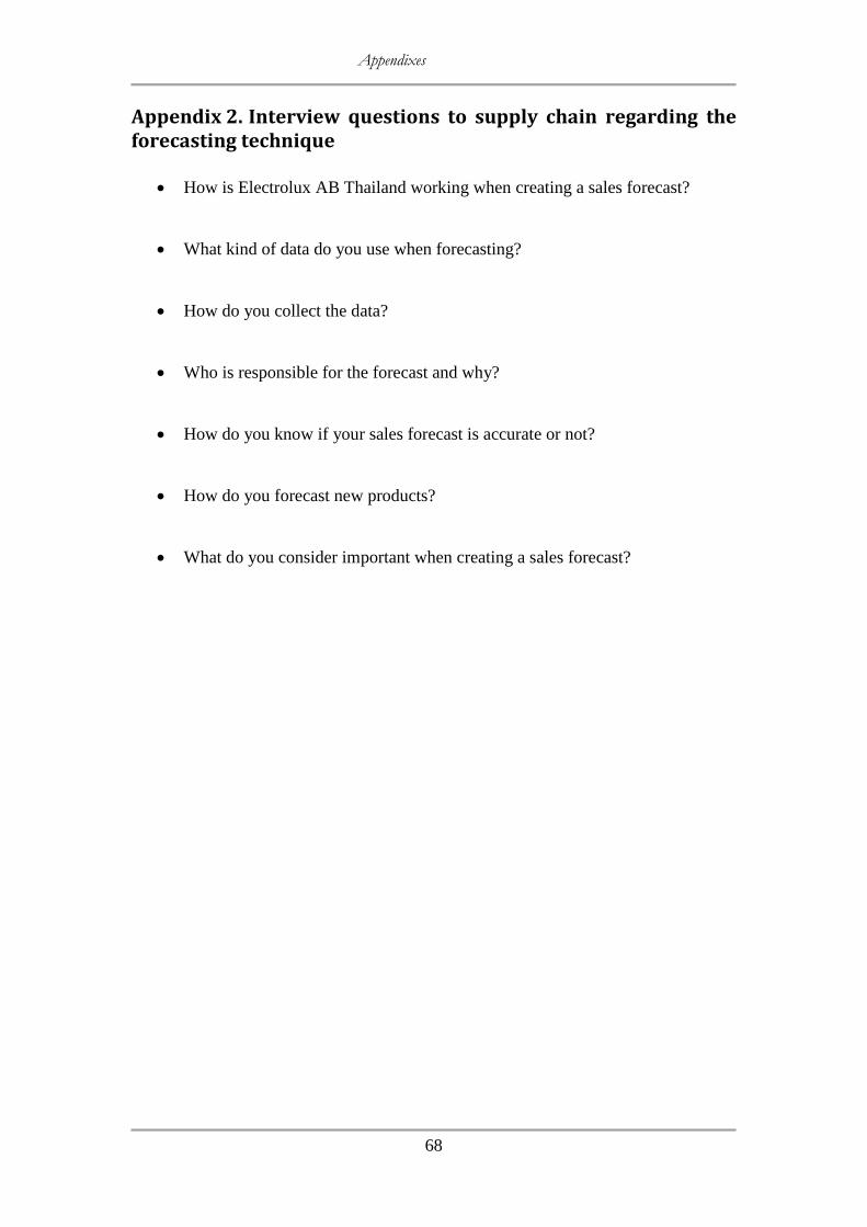
Appendixes
68
Appendix 2. Interview questions to supply chain regarding the forecasting technique
How is Electrolux AB Thailand working when creating a sales forecast?
What kind of data do you use when forecasting?
How do you collect the data?
Who is responsible for the forecast and why?
How do you know if your sales forecast is accurate or not?
How do you forecast new products?
What do you consider important when creating a sales forecast?
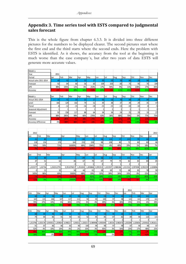
Appendixes
69
Appendix 3. Time series tool with ESTS compared to judgmental sales forecast This is the whole figure from chapter 6.3.3. It is divided into three different pictures for the numbers to be displayed clearer. The second pictures start where the first end and the third starts where the second ends. Here the problem with ESTS is identified. As it shows, the accuracy from the tool at the beginning is much worse than the case company´s, but after two years of data ESTS will generate more accurate values.
Model y
Year 2011
Period Jan Feb Mar Apr May Jun Jul Aug Sep Oct Nov Dec
Actual sales 2011-2014 49 41 59 53 17 93 53 76 84 29 84 106
Forecast 92 84 66 56 60 109 103 83 75 95 70 194
APE 88% 105% 12% 6% 253% 17% 94% 9% 11% 228% 17% 83%
Accuracy 12% -5% 88% 94% -153% 83% 6% 91% 89% -128% 83% 17%
Model y Jan Feb Mar Apr May Jun Jul Aug Sep Oct Nov Dec
Actual 2011-2014 49 41 59 53 17 93 53 76 84 29 84 106
Level 166 129 102 79 52 49 38 37 39 29 35 47
Trend -8 -12 -15 -16 -18 -15 -15 -13 -10 -10 -8 -5
Seasonal Adjustment 1 1 1 1 1 1 1 1 1 1 1 1
Forecast 92 158 117 88 64 34 34 24 25 29 19 27
APE 88% 285% 98% 66% 276% 63% 36% 68% 70% 0% 77% 75%
Accuracy 12% -185% 2% 34% -176% 37% 64% 32% 30% 100% 23% 25%
Accuracy difference 0% -180% -86% -60% -24% -46% 58% -59% -60% 228% -61% 8%
2012 2013
Jan Feb Mar Apr May Jun Jul Aug Sep Oct Nov Dec Jan
61 80 103 1 139 75 56 113 57 101 79 68 95
118 154 176 164 233 228 98 108 80 72 80 80 88
93% 93% 71% 16300% 68% 204% 75% 4% 40% 29% 1% 18% 7%
7% 8% 29% -16200% 32% -104% 25% 96% 60% 71% 99% 82% 93%
Jan Feb Mar Apr May Jun Jul Aug Sep Oct Nov Dec Jan
61 80 103 1 139 75 56 113 57 101 79 68 95
47 52 62 46 67 70 67 79 75 82 83 80 85
-4 -3 -1 -3 1 1 0 2 1 2 2 1 2
1,015577 1,02736 1,032512791 0,951076017 1,053265 1,003866 0,991913 1,021937 0,988186 1,011552 0,997698 0,992239 1,020896
-3 11 32 34 44 61 38 69 72 68 85 78 90
105% 86% 69% 3300% 68% 19% 32% 39% 26% 33% 8% 15% 5%
-5% 14% 31% -3200% 32% 81% 68% 61% 74% 67% 92% 85% 95%
-11% 6% 2% 13000% -1% 185% 43% -35% 14% -4% -6% 3% 2%
2014
Feb Mar Apr May Jun Jul Aug Sep Oct Nov Dec Jan Feb Mar Apr
60 84 96 108 80 92 91 97 53 94 66 113 108 161 116
102 115 106 107 117 111 94 93 100 97 98 141 141 170 161
70% 37% 10% 1% 46% 21% 3% 4% 89% 3% 48% 25% 31% 6% 39%
30% 63% 90% 99% 54% 79% 97% 96% 11% 97% 52% 75% 69% 94% 61%
Feb Mar Apr May Jun Jul Aug Sep Oct Nov Dec Jan Feb Mar Apr
60 84 96 108 80 92 91 97 53 94 66 113 108 161 116
79 80 86 91 90 92 92 95 85 87 82 89 94 110 115
1 1 1 2 1 2 1 2 0 0 -1 1 1 3 4
1,013796 1,033178 0,959351 1,059824 0,998217 0,99251 1,020217 0,989998 0,992049 1,00156 0,982675 1,033289 1,020656 1,054562 0,961611
91 87 86 86 83 90 100 94 98 97 99 87 90 84 87
52% 4% 10% 20% 4% 2% 10% 3% 85% 3% 50% 23% 17% 48% 25%
48% 96% 90% 80% 96% 98% 90% 97% 15% 97% 50% 77% 83% 52% 75%
18% 33% 0% -19% 43% 18% -7% 1% 4% 0% -2% 2% 14% -42% 14%

Appendixes
70